danish meteorological institute - dmi · seasonal periods reaching 0.5 mm day¡1 for the winter...

Danish Meteorological InstituteMinistry of Climate and Energy

Copenhagen 2010www.dmi.dk/dmi/dkc10-03 page 1 of 14

Danish Climate Centre Report 10-03

Weighted scenario temperature and precipitation changesfor Denmark using probability density functions forENSEMBLES regional climate models

Fredrik Boberg

−2 −1 0 1 2 3 4 5 6 7 80

0.005

0.01

0.015

0.02

∆ T [ °C]

norm

aliz

ed P

DF

DJFMAMJJASON

Danish Meteorological InstituteDanish Climate Centre Report 10-03

ColophoneSerial title:Danish Climate Centre Report 10-03

Title:Weighted scenario temperature and precipitation changes for Denmark using probability densityfunctions for ENSEMBLES regional climate models

Subtitle:

Authors:Fredrik Boberg

Other Contributers:

Responsible Institution:Danish Meteorological Institute

Language:English

Keywords:Precipitation, temperature, ENSEMBLES, regional climate modelling, probability density function

Url:http://ensemblesrt3.dmi.dk/

ISSN:1399-1957

ISBN:978-87-7478-591-0

Version:1

Website:www.dmi.dk

Copyright:Danish Meteorological Institute

www.dmi.dk/dmi/dkc10-03 page 2 of 14


ContentsColophone . . . . . . . . . . . . . . . . . . . . . . . . . . . . . . . . . . . . . . . . . . . . 21 Dansk resumé 42 Abstract 43 Introduction 44 Data 55 PDF calculation 56 Results 67 Conclusions 98 Previous reports 14



1. Dansk resuméVi bruger 19 regionale klimamodeller med en 25 km opløsning i ENSEMBLES-projektet for atestimere nedbørs- og temperaturændringer for forskellige byer i Danmark for to forskelligescenarie-perioder (2021-2050 og 2071-2099) i forhold til kontrolperioden 1961-1990. Det vægtedemodelgennemsnit af nedbørs- og temperaturændringer vises for alle fire årstider medGaussisk-filtrerede sandsynlighedsfordelinger. Modelvægtningen er baseret på modelresultater fraen særskilt undersøgelse med ERA40-forcerede simuleringer og et griddet observationsdatasæt forkontrolperioden 1961-1990. Alle danske byer der er medtaget i denne undersøgelse viser cirka densamme temperaturstigning fordelt omkring 1.5 ◦C for alle årstider for perioden 2021-2050. Forperioden 2071-2099 viser undersøgelsen en bredere fordeling med en temperaturstigning på cirka3 ◦C for alle årstider samt en sekundær top fordelt omkring 5 ◦C. For nedbørsfordelingen ser vi kunsmå positive ændringer på cirka 0.1 mm dag−1 for 2021-2050 med den største ændring om vinteren.I perioden 2071-2099 ser vi en negativ ændring på cirka 0.1 mm dag−1 for sommerperioden og enpositiv ændring for de tre andre sæsoner på cirka 0.5 mm dag−1. Disse sandsynlighedsfordelingerfor nedbør og temperatur er desuden samlet i bivariate funktioner.

2. AbstractWe use 19 25 km resolution regional climate models within the ENSEMBLES project to estimateprecipitation and temperature changes for different cities in Denmark for two different scenarioperiods (2021–2050 and 2071–2099) relative to the reference period 1961–1990. The weightedmodel means of precipitation and temperature changes are presented for all four seasons usinggaussian filtered probability density functions. The model weights are based on their performance ina separate study using ERA40 driven simulations and a gridded observational data set for the period1961–2000. All Danish cities included in this study show similar results with a temperaturedistribution around 1.5 ◦C for all seasons for the early scenario period and a more wideneddistribution around 3 ◦C for all seasons for the later scenario period including a second peak around5 ◦C. For the precipitation distribution, we see only small positive changes of a few 0.1 mm day−1

for the early scenario period with the largest change in winter. For the later period we see a negativechange of a few 0.1 mm day−1 for the summer period and a positive change for the other threeseasonal periods reaching 0.5 mm day−1 for the winter period. These probability density functionsfor precipitation and temperature are further combined into bivariate functions.

3. IntroductionThere is a large public interest for how the climate will change during the 21st century. Precipitationamounts and temperature are expected to increase globally as the climate warms due to humanactivities. Furthermore, the increases in extremes are likely to be larger than those in their means. Inthis report, we will focus on local climate changes in Denmark using a few selected cities (seeFigure 3.1). The idea is to produce probability distribution functions (PDFs) for precipitation andtemperature changes using regional climate models (RCMs). To improve the statistical significance,we use all currently available RCMs with a spatial resolution of 25 km within the ENSEMBLESproject and attach weights to each model PDF according to their performance taken fromChristensen et al. (2010). The temperature and precipitation changes are calculated by subtractingthe reference values from the scenario values, and the scenario period is divided into two periods,2021–2050 and 2071–2099.



Figure 3.1: Map of Denmark with cities used in this study highlighted. A: Copenhagen, B: Odense,C: Århus, D: Esbjerg and E: Ronne (Bornholm). Also, the entire land region of Denmark, excludingBornholm, is used as one final location.

With a spatial resolution of 25 km for the RCMs and the fact that we are only looking at a veryrestricted part of the models with a uniform climatology, we are not expecting any large differencesin PDF change for the different Danish locations (see Figure 3.1).

4. DataA total of 19 RCM simulations are currently available within the ENSEMBLES project (Hewitt,2005) at a 25 km resolution for the A1B forcing scenario (Nakicenovic et al., 2000). These RCMsare listed in Table 4.1 together with their driving models, the extent of their simulations and theirmodel weights according to Christensen et al. (2010). Models 3, 5, 10, 17 and 18 were not used byChristensen et al. (2010) so we applied weights to these models according to their neighboringmodels using a different driving GCM (see Table 4.1). This study uses seasonal (DJF, MAM, JJA,SON) means of 2m temperature and precipitation.

5. PDF calculationProbability density functions are calculated for all four seasons (DJF, MAM, JJA and SON) usingseasonal means of daily precipitation and 2m temperature from 19 RCMs. The reference period isdefined as 1961–1990 whereas the two scenario periods are defined as 2021–2050 and 2071–2099.Data for the year 2100 have been omitted as some of the models extending to the end of the 21st

century stopped their simulation in 2099 (see Table 4.1).

The PDF calculations presented here are based on the work by Déqué (2009), where 16 simulationswithin the ENSMBLES project were used for the 2021–2050 scenario period. Déqué (2009)calculated monovariate and bivariate PDFs for 32 European capitals whereas we only do calculationsfor cities in Denmark. We also decided to use a second, later, scenario period and also to remove allsea grid points before finding the grid point closest to the city in question. We furthermore define thewinter season as a contiuous DJF period and not the three winter months JFD belonging to the same



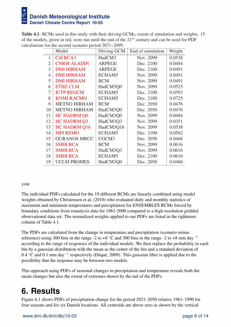
Table 4.1: RCMs used in this study with their driving GCMs, extent of simulation and weights. 15of the models, given in red, were run until the end of the 21st century and can be used for PDFcalculations for the second scenario period 2071–2099.

Model Driving GCM End of simulation Weight1 C4I RCA3 HadCM3 Nov. 2099 0.05382 CNRM ALADIN ARPEGE Dec. 2100 0.04843 DMI HIRHAM ARPEGE Dec. 2100 0.04914 DMI HIRHAM ECHAM5 Nov. 2099 0.04915 DMI HIRHAM BCM Nov. 2099 0.04916 ETHZ CLM HadCM3Q0 Nov. 2099 0.05237 ICTP REGCM ECHAM5 Dec. 2100 0.05938 KNMI RACMO ECHAM5 Dec. 2100 0.07259 METNO HIRHAM BCM Dec. 2050 0.0476

10 METNO HIRHAM HadCM3Q0 Dec. 2050 0.047611 HC HADRM Q0 HadCM3Q0 Nov. 2099 0.048412 HC HADRM Q3 HadCM3Q3 Nov. 2099 0.035113 HC HADRM Q16 HadCM3Q16 Nov. 2099 0.053814 MPI REMO ECHAM5 Dec. 2100 0.056215 OURANOS MRCC CGCM3 Dec. 2050 0.046816 SMHI RCA BCM Nov. 2099 0.061617 SMHI RCA HadCM3Q3 Nov. 2099 0.061618 SMHI RCA ECHAM5 Dec. 2100 0.061619 UCLM PROMES HadCM3Q0 Dec. 2050 0.0460

year.

The individual PDFs calculated for the 19 different RCMs are linearly combined using modelweights obtained by Christensen et al. (2010) who evaluated daily and monthly statistics ofmaximum and minimum temperatures and precipitation for ENSEMBLES RCMs forced byboundary conditions from reanalysis data for 1961-2000 compared to a high-resolution griddedobservational data set. The normalized weights applied to our PDFs are listed in the rightmostcolumn of Table 4.1.

The PDFs are calculated from the change in temperature and precipitation (scenario minusreference) using 300 bins in the range -2 to +8 ◦C and 300 bins in the range -2 to +8 mm day−1

according to the range of responses of the individual models. We then replace the probability in eachbin by a gaussian distribution with the mean as the center of the bin and a standard deviation of0.4 ◦C and 0.1 mm day−1 respectively (Déqué, 2009). This gaussian filter is applied due to thepossibility that the response may be between two models.

This approach using PDFs of seasonal changes in precipitation and temperature reveals both themean changes but also the extent of extremes shown by the tail of the PDFs.

6. ResultsFigure 6.1 shows PDFs of precipitation change for the period 2021–2050 relative 1961–1990 forfour seasons and for six Danish locations. All centroids are above zero as shown by the vertical



−2 −1.5 −1 −0.5 0 0.5 1 1.5 20

0.01

0.02

0.03

0.04

0.05

0.06

0.07

∆ P [mm day−1]

norm

aliz

ed P

DF

aDJFMAMJJASON

−2 −1.5 −1 −0.5 0 0.5 1 1.5 20

0.01

0.02

0.03

0.04

0.05

0.06

0.07

∆ P [mm day−1]

norm

aliz

ed P

DF

bDJFMAMJJASON

−2 −1.5 −1 −0.5 0 0.5 1 1.5 20

0.01

0.02

0.03

0.04

0.05

0.06

0.07

∆ P [mm day−1]

norm

aliz

ed P

DF

cDJFMAMJJASON

−2 −1.5 −1 −0.5 0 0.5 1 1.5 20

0.01

0.02

0.03

0.04

0.05

0.06

0.07

∆ P [mm day−1]

norm

aliz

ed P

DF

dDJFMAMJJASON

−2 −1.5 −1 −0.5 0 0.5 1 1.5 20

0.01

0.02

0.03

0.04

0.05

0.06

0.07

∆ P [mm day−1]

norm

aliz

ed P

DF

eDJFMAMJJASON

−2 −1.5 −1 −0.5 0 0.5 1 1.5 20

0.01

0.02

0.03

0.04

0.05

0.06

0.07

∆ P [mm day−1]

norm

aliz

ed P

DF

fDJFMAMJJASON

Figure 6.1: Probability density functions for precipitation response 2021–2050 relative 1961–1990using seasonal mean data for a: Copenhagen, b: Odense, c: Århus, d: Esbjerg, e: Bornholm and f:Denmark. The centroids for each PDF is given by a corresponding vertical line at the bottom of eachpanel.

colored lines at the bottom of each panel. The change in precipitation is largest for the winter seasonwith about 0.25 mm day−1. The PDFs for Esbjerg are wider that the other PDFs. The summer PDFsshow, on average, the smallest change.

Figure 6.2 shows PDFs of precipitation change for the period 2071–2099 relative 1961–1990 forfour seasons and for six Danish locations. The PDFs for the summer season now show a clearnegative change for some locations whereas the PDFs for the other three seasons show a positivechange. The DJF and SON PDFs have centroids around 0.45 mm day−1. The PDFs also show somesecondary peaks, especially for the SON period on the left wing.

Figure 6.3 shows PDFs of temperature change for the period 2021–2050 relative 1961–1990. Allcentroids are between 1 and 2 ◦C. The change in temperature is largest for the winter season. The



−2 −1.5 −1 −0.5 0 0.5 1 1.5 20

0.01

0.02

0.03

0.04

0.05

0.06

0.07

∆ P [mm day−1]

norm

aliz

ed P

DF

aDJFMAMJJASON

−2 −1.5 −1 −0.5 0 0.5 1 1.5 20

0.01

0.02

0.03

0.04

0.05

0.06

0.07

∆ P [mm day−1]

norm

aliz

ed P

DF

bDJFMAMJJASON

−2 −1.5 −1 −0.5 0 0.5 1 1.5 20

0.01

0.02

0.03

0.04

0.05

0.06

0.07

∆ P [mm day−1]

norm

aliz

ed P

DF

cDJFMAMJJASON

−2 −1.5 −1 −0.5 0 0.5 1 1.5 20

0.01

0.02

0.03

0.04

0.05

0.06

0.07

∆ P [mm day−1]

norm

aliz

ed P

DF

dDJFMAMJJASON

−2 −1.5 −1 −0.5 0 0.5 1 1.5 20

0.01

0.02

0.03

0.04

0.05

0.06

0.07

∆ P [mm day−1]

norm

aliz

ed P

DF

eDJFMAMJJASON

−2 −1.5 −1 −0.5 0 0.5 1 1.5 20

0.01

0.02

0.03

0.04

0.05

0.06

0.07

∆ P [mm day−1]

norm

aliz

ed P

DF

fDJFMAMJJASON

Figure 6.2: Probability density functions for precipitation response 2071–2099 relative 1961–1990using seasonal mean data for a: Copenhagen, b: Odense, c: Århus, d: Esbjerg, e: Bornholm and f:Denmark. The centroids for each PDF is given by a corresponding vertical line at the bottom of eachpanel.

PDFs for the MAM and SON periods match each other well. Only a small part of the PDFdistributions extend to negative temperature changes.

Figure 6.4 shows PDFs of temperature change for the period 2071–2099 relative 1961–1990. Allcentroids are now located around 3 ◦C. The change in temperature is still largest for the winterseason and the smallest change is seen in summer. As in the case of precipitation for the laterscenario period, we see clear secondary peaks. However, these peaks are now on the right wing ofthe distribution and seen for both the SON and the DJF period around 5 ◦C.

Figures 6.5 and 6.6 shows bivariate PDFs of temperature and precipitation change for the periods2021–2050 and 2051-2099 relative 1961–1990, respectively. Each location is represented by fourpanels, one for each season.



−2 −1 0 1 2 3 4 5 6 7 80

0.005

0.01

0.015

0.02

∆ T [ °C]

norm

aliz

ed P

DF

a DJFMAMJJASON

−2 −1 0 1 2 3 4 5 6 7 80

0.005

0.01

0.015

0.02

∆ T [ °C]

norm

aliz

ed P

DF

b DJFMAMJJASON

−2 −1 0 1 2 3 4 5 6 7 80

0.005

0.01

0.015

0.02

∆ T [ °C]

norm

aliz

ed P

DF

c DJFMAMJJASON

−2 −1 0 1 2 3 4 5 6 7 80

0.005

0.01

0.015

0.02

∆ T [ °C]

norm

aliz

ed P

DF

d DJFMAMJJASON

−2 −1 0 1 2 3 4 5 6 7 80

0.005

0.01

0.015

0.02

∆ T [ °C]

norm

aliz

ed P

DF

e DJFMAMJJASON

−2 −1 0 1 2 3 4 5 6 7 80

0.005

0.01

0.015

0.02

∆ T [ °C]

norm

aliz

ed P

DF

f DJFMAMJJASON

Figure 6.3: Probability density functions for temperature response 2021–2050 relative 1961–1990using seasonal mean data for a: Copenhagen, b: Odense, c: Århus, d: Esbjerg, e: Bornholm and f:Denmark. The centroids for each PDF is given by a corresponding vertical line at the bottom of eachpanel.

Finally, in Figure 6.7, we show how the bivariate PDFs of temperature and precipitation change foroverlapping three-month periods during the course of the year for the later scenario period relative1961–1990 for the Denmark region. We only show the outer 95% confidence level for eachthree-month period (cf. Figure 6.6). Also shown are the centroids for each three-month period. Thecentroids, with its slanted hour-glass shape when combined, are only negative in precipitation for thetwo summer periods JJA and JAS.

7. ConclusionsBy linearly combining PDFs for 19 RCMs within the ENSEMBLES project, we have determined thedistributional change for seasonal mean temperature and precipitation for a few selected cities inDenmark for two scenario periods (2021–2050 and 2071–2099) relative to the reference period



−2 −1 0 1 2 3 4 5 6 7 80

0.005

0.01

0.015

0.02

∆ T [ °C]

norm

aliz

ed P

DF

a DJFMAMJJASON

−2 −1 0 1 2 3 4 5 6 7 80

0.005

0.01

0.015

0.02

∆ T [ °C]

norm

aliz

ed P

DF

b DJFMAMJJASON

−2 −1 0 1 2 3 4 5 6 7 80

0.005

0.01

0.015

0.02

∆ T [ °C]

norm

aliz

ed P

DF

c DJFMAMJJASON

−2 −1 0 1 2 3 4 5 6 7 80

0.005

0.01

0.015

0.02

∆ T [ °C]

norm

aliz

ed P

DF

d DJFMAMJJASON

−2 −1 0 1 2 3 4 5 6 7 80

0.005

0.01

0.015

0.02

∆ T [ °C]

norm

aliz

ed P

DF

e DJFMAMJJASON

−2 −1 0 1 2 3 4 5 6 7 80

0.005

0.01

0.015

0.02

∆ T [ °C]

norm

aliz

ed P

DF

f DJFMAMJJASON

Figure 6.4: Probability density functions for temperature response 2071–2099 relative 1961–1990using seasonal mean data for a: Copenhagen, b: Odense, c: Århus, d: Esbjerg, e: Bornholm and f:Denmark. The centroids for each PDF is given by a corresponding vertical line at the bottom of eachpanel.

1961–1990. The combination is done using the model weights obtained in a separate study(Christensen et al., 2010) and the monovariate and bivariate distributions show both the mean changebut also the extent of extreme changes. The sign of the changes are statistically significant fortemperature only (both scenario periods), and to some extent also for DJF precipitation for the latescenario period. For the other seasons during the late scenario period and for all seasons for the earlyperiod, the sign of the precipitation response is never significant since there is always a significantprobability that the sign is positive or negative.

Acknowledgements The ENSEMBLES project (contract number GOCE-CT-2003-505539) issupported by the European Commission’s 6th Framework Programme as a 5 year Integrated Projectfrom 2004–2009 under the Thematic Sub-Priority ”Global Change and Ecosystems”. The author



DJF

a

∆ T [ °C]

∆ P

[mm

day

−1 ]

0 2 4 6

−1

0

1

MAM

∆ T [ °C]

∆ P

[mm

day

−1 ]

0 2 4 6

−1

0

1

JJA

∆ T [ °C]

∆ P

[mm

day

−1 ]

Confidence levels [%]

0 2 4 6

−1

0

1

95 80 60 40 20

SON

∆ T [ °C]

∆ P

[mm

day

−1 ]

0 2 4 6

−1

0

1

DJF

b

∆ T [ °C]

∆ P

[mm

day

−1 ]

0 2 4 6

−1

0

1

MAM

∆ T [ °C]

∆ P

[mm

day

−1 ]

0 2 4 6

−1

0

1

JJA

∆ T [ °C]

∆ P

[mm

day

−1 ]


0 2 4 6

−1

0

1

95 80 60 40 20

SON

∆ T [ °C]

∆ P

[mm

day

−1 ]

0 2 4 6

−1

0

1

DJF

c

∆ T [ °C]

∆ P

[mm

day

−1 ]

0 2 4 6

−1

0

1

MAM

∆ T [ °C]

∆ P

[mm

day

−1 ]

0 2 4 6

−1

0

1

JJA

∆ T [ °C]

∆ P

[mm

day

−1 ]


0 2 4 6

−1

0

1

95 80 60 40 20

SON

∆ T [ °C]

∆ P

[mm

day

−1 ]

0 2 4 6

−1

0

1

DJF

d

∆ T [ °C]∆

P [m

m d

ay−

1 ]

0 2 4 6

−1

0

1

MAM

∆ T [ °C]

∆ P

[mm

day

−1 ]

0 2 4 6

−1

0

1

JJA

∆ T [ °C]

∆ P

[mm

day

−1 ]


0 2 4 6

−1

0

1

95 80 60 40 20

SON

∆ T [ °C]

∆ P

[mm

day

−1 ]

0 2 4 6

−1

0

1

DJF

e

∆ T [ °C]

∆ P

[mm

day

−1 ]

0 2 4 6

−1

0

1

MAM

∆ T [ °C]

∆ P

[mm

day

−1 ]

0 2 4 6

−1

0

1

JJA

∆ T [ °C]

∆ P

[mm

day

−1 ]


0 2 4 6

−1

0

1

95 80 60 40 20

SON

∆ T [ °C]

∆ P

[mm

day

−1 ]

0 2 4 6

−1

0

1

DJF

f

∆ T [ °C]

∆ P

[mm

day

−1 ]

0 2 4 6

−1

0

1

MAM

∆ T [ °C]

∆ P

[mm

day

−1 ]

0 2 4 6

−1

0

1

JJA

∆ T [ °C]

∆ P

[mm

day

−1 ]


0 2 4 6

−1

0

1

95 80 60 40 20

SON

∆ T [ °C]

∆ P

[mm

day

−1 ]

0 2 4 6

−1

0

1

Figure 6.5: Confidence contours of bivariate probability density functions for temperature andprecipitation response 2021–2050 relative 1961–1990 for a: Copenhagen, b: Odense, c: Århus, d:Esbjerg, e: Bornholm and f: Denmark. While the contours are shown relative the peak probability,the centroids for each PDF and for each season are marked by an ’x’ in each subpanel.

wish to thank Michel Déqué for the PDF calculation scripts.

References

Christensen J.H., Kjellström, E., Giorgi, F., Lenderink, G., Rummukainen, M. Weight assignment inregional climate models, Climate Research, 44:179–194, doi: 10.3354/cr00916, 2010.

Déqué, M. Temperature and precipitation probability density functions in ENSEMBLES regionalscenarios, ENSEMBLES technical report no. 5, 2009.



DJF

a

∆ T [ °C]

∆ P

[mm

day

−1 ]

0 2 4 6

−1

0

1

MAM

∆ T [ °C]

∆ P

[mm

day

−1 ]

0 2 4 6

−1

0

1

JJA

∆ T [ °C]

∆ P

[mm

day

−1 ]


0 2 4 6

−1

0

1

95 80 60 40 20

SON

∆ T [ °C]

∆ P

[mm

day

−1 ]

0 2 4 6

−1

0

1

DJF

b

∆ T [ °C]

∆ P

[mm

day

−1 ]

0 2 4 6

−1

0

1

MAM

∆ T [ °C]

∆ P

[mm

day

−1 ]

0 2 4 6

−1

0

1

JJA

∆ T [ °C]

∆ P

[mm

day

−1 ]


0 2 4 6

−1

0

1

95 80 60 40 20

SON

∆ T [ °C]

∆ P

[mm

day

−1 ]

0 2 4 6

−1

0

1

DJF

c

∆ T [ °C]

∆ P

[mm

day

−1 ]

0 2 4 6

−1

0

1

MAM

∆ T [ °C]

∆ P

[mm

day

−1 ]

0 2 4 6

−1

0

1

JJA

∆ T [ °C]

∆ P

[mm

day

−1 ]


0 2 4 6

−1

0

1

95 80 60 40 20

SON

∆ T [ °C]

∆ P

[mm

day

−1 ]

0 2 4 6

−1

0

1

DJF

d

∆ T [ °C]∆

P [m

m d

ay−

1 ]

0 2 4 6

−1

0

1

MAM

∆ T [ °C]

∆ P

[mm

day

−1 ]

0 2 4 6

−1

0

1

JJA

∆ T [ °C]

∆ P

[mm

day

−1 ]


0 2 4 6

−1

0

1

95 80 60 40 20

SON

∆ T [ °C]

∆ P

[mm

day

−1 ]

0 2 4 6

−1

0

1

DJF

e

∆ T [ °C]

∆ P

[mm

day

−1 ]

0 2 4 6

−1

0

1

MAM

∆ T [ °C]

∆ P

[mm

day

−1 ]

0 2 4 6

−1

0

1

JJA

∆ T [ °C]

∆ P

[mm

day

−1 ]


0 2 4 6

−1

0

1

95 80 60 40 20

SON

∆ T [ °C]

∆ P

[mm

day

−1 ]

0 2 4 6

−1

0

1

DJF

f

∆ T [ °C]

∆ P

[mm

day

−1 ]

0 2 4 6

−1

0

1

MAM

∆ T [ °C]

∆ P

[mm

day

−1 ]

0 2 4 6

−1

0

1

JJA

∆ T [ °C]

∆ P

[mm

day

−1 ]


0 2 4 6

−1

0

1

95 80 60 40 20

SON

∆ T [ °C]

∆ P

[mm

day

−1 ]

0 2 4 6

−1

0

1

Figure 6.6: Confidence contours of bivariate probability density functions for temperature andprecipitation response 2071–2099 relative 1961–1990 for a: Copenhagen, b: Odense, c: Århus, d:Esbjerg, e: Bornholm and f: Denmark. While the contours are shown relative the peak probability,the centroids for each PDF and for each season are marked by an ’x’ in each subpanel.

Hewitt, C. D. The ENSEMBLES Project: Providing ensemble-based predictions of climate changesand their impacts, EGGS newsletter 13:22–25, 2005.

Nakicenovic, N., Alcamo, J., Davis, J., de Vries, B., Fenhann, J., Gaffin, S., Gregory, K., Grübler,A., Jung, TY., Kram, T., Lebre La Rovere, E., Michaelis, L., Mori, S., Morita, T., Pepper, W.,Pitcher, H., Price, L., Riahi, K., Roehrl, A., Rogner, H.-H., Sankovski, A., Schlesinger, M.,Shukla, P., Smith, S., Swart, R., van Rooijen, S., Victor, N., Dadi, Z. Special report on emissionscenarios, A special report of Working Group III for the Intergovernmental Panel on ClimateChange, Cambridge University Press, 2000.



01

23

45

6

−1

−0.

50

0.51

∆ T

[ ° C

]

∆ P [mm day−1

]

DJF

JFM

FM

AM

AM

AM

JM

JJJJ

AJA

SA

SO

SO

NO

ND

ND

J

Figure 6.7: 95 percent confidence contours of bivariate probability density functions for temperatureand precipitation response 2071–2099 relative 1961–1990 for Denmark. Each contour represents athree-month ("seasonal") mean for the overlapping periods DJF, JFM, FMA, ..., NDJ. The centroidsfor each three-month period are marked by an ’x’. Note that the axis limits are not the same as forFigures 6.5 and 6.6



8. Previous reportsPrevious reports from the Danish Meteorological Institute can be found on:http://www.dmi.dk/dmi/dmi-publikationer.htm


danish meteorological institute - dmi · seasonal periods reaching 0.5 mm day¡1 for the winter...

Documents