data analysis & modeling techniques statistics and

© Manfred Huber 2017 1

Data Analysis & Modeling Techniques

Statistics and Hypothesis Testing


Hypothesis Testing

n  Hypothesis testing is a statistical method used to evaluate if a particular hypothesis about data resulting from an experiment is reasonable. n  Uses statistics to represent the data

n  Value of the data

n  Distribution of the data

n  Determine how likely it is that a given hypothesis about the data is correct


Hypothesis Testing n  Hypothesis testing is aimed at establishing if a particular

hypothesis about a set of observations (data) should be trusted n  Example:

n  The average and variance of the body height of the population of a country is

n  In a different country a set of 10 people are randomly selected and measured resulting in the following data set with mean = 1.776:

n  Can we conclude that people in this second country are on the average taller (average height μX) than people in the first one ?

01.0,7.1 2 == σµ

}7.1,65.1,75.1,82.1,77.1,7.1,75.1,92.1,9.1,8.1{X


Hypothesis Testing n  To be able to trust in a hypothesis on statistical data

we have to make sure that the data set could not be the result of random chance n  In the example the hypothesis would be:

n  To determine if the hypothesis has a base we have to make sure that we do not accept it if the data could be the result of random chance

n  What is the likelihood that the data could be obtained by randomly sampling 10 items from the distribution in the first country ?

µµ >XH :


Percentiles n  To determine the likelihood that a data item could

come from a distribution we have to be able to determine percentiles n  A data item belongs to the nth percentile if the likelihood to

obtain a value that is equal to the data item or even further away from the distribution mean is greater or equal to n%

n  For certain distributions (e.g. normal distribution) percentiles can be relatively easily calculated


Percentiles in Normal Distributions

n  The percentile in a normal distribution is a function of the distance of the data value from the mean and of the standard deviation

n  E.g. a data value that is more than 1.5 standard deviations larger than the mean of the distribution occurs only with probability 0.0668

σµ−

=Xz


Percentiles n  If the distribution of the population is normal, the

z-value and the z-table allow to compute how likely it would be to randomly draw the particular data value (or one even further from the mean) n  If the likelihood is not very small, then we should not

assume that the data value is significant different from the value of the distribution

n  Percentiles for general, skewed distributions are difficult to derive n  Attempt to formulate hypothesis on a statistic for which

the distribution is approximately normal


Sampling Distributions n  Sample Distribution: The probability distribution

representing individual data items

n  Sampling Distribution: The probability distribution of a statistic calculated from a set of randomly drawn data items n  Sampling Distribution of the mean: The distribution of the

means of random data samples of size n n  For a sample distribution with mean μ and standard

deviation σ the mean μs and standard deviation σs of the sampling distribution of the mean over n samples is:

nssσ

σµµ == ,


Central Limit Theorem n  For any sample distribution with mean μ and

standard deviation σ , the sampling distribution of the mean approaches a normal distribution with mean μ and standard deviation σ/√n as n becomes larger n  Percentiles for the sampling

distribution of the mean are

easier to compute than for

the sample distribution.


Logic of Hypothesis Testing n  The goal of hypothesis testing is to establish the viability of a

hypothesis about a parameter of the population (often the mean) n  Define hypothesis (also called alternative hypothesis)

n  E.g.:

n  Set up Null hypothesis (i.e. the “opposite” of the hypothesis) n  E.g.:

n  Compute the percentile and thus the likelihood of the Null hypothesis

n  If the Null hypothesis has more than a small likelihood, the data does not significantly support the hypothesis (since it could also represent the Null hypothesis)

n  Usually thresholds or 5% or smaller are used

µµ >XAH :

µµ =XH :0


Logic of Hypothesis Testing n  If the Null hypothesis’ likelihood (i.e. the likelihood to

obtain data at least as extreme) is smaller than the significance level, the Null hypothesis can be rejected n  Rejection implies that the Null hypothesis is discarded in

favor of the alternative hypothesis and the result is considered significant

n  Note that a p-value less than 5% for the Null hypothesis does NOT imply a likelihood of 95% for the alternative hypothesis.

n  Note that it is NOT possible to show that the Null hypothesis is correct. Failure to reject the Null hypothesis does NOT imply acceptance of the Null hypothesis but rather that no significant conclusion could be drawn from the test


One-Tailed vs. Two-Tailed Tests n  Depending on the hypotheses we might be interested to know how

the likelihood to generate data that is more extreme than the test data in a particular direction (e.g. the likelihood of it being larger than or equal to the given data) or in any direction (i.e. that it is further from the mean than the given data)

n  If we are only interested in data on one end of

the distribution we perform a one-tailed test,

i.e. we only count the percentile at one end of

the distribution

n  If we are interested in both sides, we perform a

two-tailed test which computes the percentile at

both ends

n  If we are not sure we should choose a two-tailed test (which is more stringent)


The Z Test n  The Z Test is the most basic hypothesis test to evaluate a hypothesis

relating an unknown distribution (with mean μX) from which a known sample set {Xi} of size n with mean was randomly drawn to a population with sample distribution with mean μ and standard deviation σ

n  Assumes that the sampling distribution of the means is normal n  Either the sample distribution is normal or the sample size is very large

n  Example Hypotheses:

n  Compute z-value:

n  Translate z-value to p-value and evaluate significance n  Translation usually uses z-table. E.g. p = 2.5% -> z=1.96

X

µµ

µµ

>

=

HA

H

HH::0

nXzσ

µ−=


Z Test With Unknown Variance n  If the standard deviation of the population is unknown we can

make the assumption that the population and the data set have come from populations with the same standard deviation

n  Use standard error s of the sample set to estimate standard deviation of the sampling distribution

n  Compute z-value:

n  Translate z-value to p-value and evaluate significance n  Translation usually uses z-table. E.g. p = 2.5% -> z=1.96

nsXz µ−

=

ns

ns ≈=σ

σ


Student’s t Distribution n  If the sample size is small and the form of the

sample distribution is unknown a normal distribution might not be the correct distribution for the sampling distribution of the mean n  Student’s t distribution addresses this by increasing the

spread of the distribution as the sample size decreases n  For large sample sizes Student’s t approximates the normal

distribution arbitrarily well

n  For small sample sizes Student’s t models the deviations in the variance estimates


The t Test n  The t test operates in the same way as the Z test

but uses Student’s t distribution instead of the normal distribution n  Example Hypotheses:

n  Compute t-value:

n  Translate t-value to the corresponding p-value (percentile) according to the Student’s t distribution for sample size n and evaluate significance

n  Translation usually uses t-table. E.g. p = 2.5% -> t9=2.26

µµ

µµ

≠

=

HA

H

HH::0

nsXtn

µ−=−1


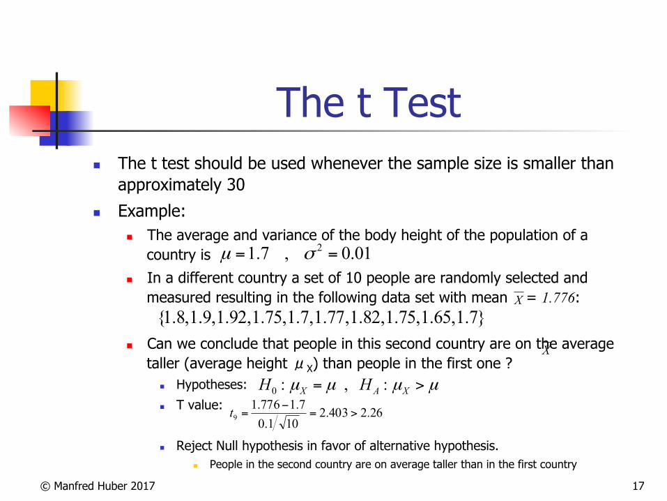
The t Test n  The t test should be used whenever the sample size is smaller than

approximately 30

n  Example: n  The average and variance of the body height of the population of a

country is

n  In a different country a set of 10 people are randomly selected and measured resulting in the following data set with mean = 1.776:

n  Can we conclude that people in this second country are on the average taller (average height μX) than people in the first one ?

n  Hypotheses:

n  T value:

n  Reject Null hypothesis in favor of alternative hypothesis. n  People in the second country are on average taller than in the first country

01.0,7.1 2 == σµ

}7.1,65.1,75.1,82.1,77.1,7.1,75.1,92.1,9.1,8.1{

µµµµ >= XAX HH :,:026.2403.2

101.07.1776.1

9 >=−

=t

X

X


Two-Sample t Test n  A two-sample test is to compare two samples to see whether they come from

the same or different distributions n  E.g.: Does algorithm 1 perform better than algorithm 2 based on a set of

experiments performed with each

n  Since no population standard deviation or mean is available, the standard error from the two samples is pooled to obtain an estimate of the standard deviation of the difference between the two sample distributions



n  Translate t-value to the corresponding p-value (percentile) according to the Student’s t distribution for n1+n2-2 degrees of freedom and evaluate significance

21210 :,: µµµµ ≠= AHH( ) ( )

2121

21

2121212

XXXXnn

XXXXt−−

−+

−=

−−−=

σσµµ

2

22

1

21

21 ns

ns

XX +=−

σ


Paired Sample t Test n  A paired sample test is used to compare two sample sets that have a different

common variable that should be controlled for to see whether they come from the same or different distributions

n  E.g.: Does algorithm 1 perform better than algorithm 2 based on their performance on a specific set of problems (the same problems for both)

n  A paired sample test avoids the variance caused by the controlled variable (e.g. the specific problem the algorithm is applied to) by establishing the sampling distribution over the differences in the value between paired data items from both sets



n  Translate t-value to the corresponding p-value (percentile) according to the Student’s t distribution for sample size n and evaluate significance

0:,0:0 >= δδ µµ AHH

nsXtnδ

δδ µ−=−1

}{ )(2

)(1

)( iii XXX −=δ


Paired Sample vs. Two-Sample Test

n  The paired sample test is preferable whenever an additional variable is known which produces variations in the data items n  Paired sample test often has smaller standard

deviations because of the avoided variance

n  If no conditional variable that would pair individual samples together is known to be relevant, the two-sample test is most of the time better because it uses more samples


Confidence Intervals n  Confidence intervals on the means of data points (or curves)

indicate intervals for which, if a data point from a different sample falls within it, a significance test would not succeed to reject the Null hypothesis. n  E.g.: The performance for system 1 is significantly better than the

performance of system 2 if the performance values lie outside the confidence intervals.

n  A (1-α)% confidence interval around a data point would cover all values for which the t-value with respect to would have a p-value below α%

n  Confidence interval bounds:

XX

⎥⎦

⎤⎢⎣

⎡+− −− n

stXnstX nn 1,1, , αα


Confidence Intervals n  When presenting and comparing performance data (and

making statements regarding performance differences) either significance test should be performed or error bars (confidence intervals) should be presented with the data n  Error bars illustrate the

significance of the difference

between two performance

measures n  Error bars usually either

represent (1-α)% confidence

intervals or are of size α


Testing Other Properties n  Z and T tests utilize the results of the central limit

theorem to allow the test of (and determination of the significance of evidence for) hypotheses about the mean of a distribution n  Since the sampling distribution for the mean is represented

by either a Student-t distribution or, if the number of samples is large enough or the sample distribution is normal, by a normal distribution

n  We can use the same approach for any other statistic for which we know the sampling distribution


Testing Variance n  Another important property of distributions is the

variance n  Variance indicates the spread of the values drawn

n  Can correspond to “reliability”, “noisiness”, etc. n  To allow significance tests about hypotheses related

to the variance we need to know what the sampling distribution of the variance of a sample distribution is and be able to compute its percentiles n  If we know this distribution, significance tests can be

performed in the same way as for the mean


Sampling Distribution of the Variance

n  The variance of a random variable can be interpreted itself as a random variable (x-μ)2

n  While we have shown that the mean and variance of the product of two independent random variables are μXμY and σX

2σY2+μX

2σY2+μY

2σX2, respectively, independent

of the distribution of the variables, this does not apply to the variance (dependent variables)

n  The distribution of the variance is specific to the distribution of the variable

n  Only for some cases are general distributions of the variance easily known and usable


The Chi-Squared Distribution n  The χk

2 -Distribution is a family of distributions of the sum of squares of k variates independently drawn from a standard normal distribution n  For k=1 this corresponds to the distribution of the variance

of a standard normal distribution. For larger k it corresponds to the distribution of the variance of a sample set of size k+1 taken from the standard normal distribution

p! 2(x;k) = x

k2"1e"

x2

2# k2( )


Chi-Squared Tests n  The χ2 –Distribution can be used in tests related to

the variance of a distribution n  If the distribution is known to be normal the χ2 value for the

correct number of degrees of freedom can be used n  To extend it to arbitrary normal distributions, it is important

to note that any normal distribution is just a shifted, stretched version of the standard normal (shifted by μ and stretched by σ)

n  For distributions of unknown shape, the distribution of the mean of samples of sufficient size is normal with mean μ and standard deviation σ/√n. χ2 thus models the variance of sample means of sufficiently large samples (after scaling)


The Chi-Squared Tests n  The χ2 test operates in the same way as the Z and

t tests but uses the χk2 distribution


n  Compute χ2-value:

n  Translate χ2-value to the corresponding p-value (percentile) according to the χ2 distribution for sample size n and evaluate significance

n  Translation usually uses χ2-table. E.g. p = 2.5% -> χ92=19.02

H0 :!2H =!

2

HA :!2H <!

2

! 2n"1 =(n "1)s2

# 2


The F-Distribution n  If the shape of the sample distribution is not known and

there are not enough samples to perform a variance test on a normal sampling distribution we need a different distribution for the variance

n  The F-distribution models the distribution of the ratio of two random variables, each drawn from a χk

2-Distribution scaled by 1/k.

n  For k1=1 and k2=n-1, the F-distribution models the distribution of the variance of samples drawn from a student-t distribution for sample size n (n-1 degrees of freedom)

pF (x;k1,k2 ) =(k1x)

k1 k2k2

(k1x + k2 )k1+k2

! k1 + k2( )x ! k1( ) + ! k2( )( )


F-Test n  There are multiple scenarios under which we can use the

F-distribution to evaluate hypotheses about the variance of a random distribution

n  F-Distribuiton F(k1,k2) models the ratio of the variances of sample sets drawn from two normal distributions.

n  F-test can evaluate how likely it is to obtain a given value for the ratio between a known normal distribution and a sample set taken from that distribution

n  F-test can evaluate the likelihood to obtain a given value for the ratio between two sample sets taken from a normal distribution.

n  F-Distribution F(1,k) models the variance of a set of samples taken from a t-distribution with k degrees of freedom


The F-Tests n  The F-test operates in the same way as the other

tests but uses the F- distribution n  Example Hypotheses:

n  Compute F-value:

n  Translate F-value to the corresponding p-value (percentile) according to the F-distribution for sample sizes n,m and evaluate significance

n  Translation usually uses F-table. E.g. p = 5% -> F9,9=3.18

H0 :!2H =!

2

HA :!2H <!

2

Fn!1,m!1 =s12

s22


Other Test Distributions n  F-tests and χ2-tests can also be used in paired scenarios

and with and without one of the test distributions being known.

n  If the variance does not fit the χ2 or the F-distribution, there are a large range of related test statistics (and distributions) that can be used

n  Many variations of the F-test

n  Likelihood ratio test

n  Anova

n  r-test

n  …


Significance Testing n  To be able to make statements comparing performance derived from

experiments it is necessary to show that the differences are not the result of chance

n  Benefits n  Significance tests are a flexible way to evaluate if a hypothesis about the

sampling mean (or some similar statistics) has significant support

n  Significance tests can be applied without complete knowledge of the distributions underlying the problem

n  Problems: n  Significance tests only reject the Null hypothesis

n  No direct proof of the hypothesis

n  Significance tests are difficult when trying to evaluate hypotheses that are not involving the mean

data analysis & modeling techniques statistics and

Documents