data analysis, statistics, machine learningwilkinson/dataanalysiscourse/session 07... · data...
TRANSCRIPT
Data Analysis, Statistics, Machine Learning
Leland Wilkinson Adjunct Professor UIC Computer Science Chief Scien<st H2O.ai [email protected]
2
Inference o Inference involves drawing conclusions from evidence
o In logic, the evidence is a set of premises o In data analysis, the evidence is a set of data o In sta<s<cs, the evidence is a sample from a popula<on
o A popula<on is assumed to have a distribu<on o The sample is assumed to be random (There are ways around that) o The popula<on may be the same size as the sample
o There are two historical approaches to sta<s<cal inference o Frequen<st o Bayesian
o There are many widespread abuses of sta<s<cal inference o We cherry pick our results (scien<sts, journals, reporters, …) o We didn’t have a big enough sample to detect a real difference o We think a large sample guarantees accuracy (the bigger the beRer)
Copyright © 2016 Leland Wilkinson
3
Inference Deduc<ve (top down)
All men are mortal. (premise) Apollo is a man. (premise) Therefore, Apollo is mortal. (conclusion) The conclusion is guaranteed if premises are true
Abduc<ve Bill and Jane had a fight and stopped seeing each other I just saw Bill and Jane having coffee together I conclude they are friends again The conclusion is not guaranteed even if premise(s) are true
Induc<ve (boRom up) o All of the swans we have seen are white. o Therefore, all swans are white.
The conclusion is not guaranteed even if premise(s) are true There exist black swans (also blue lobsters)
Mathema<cal proofs are deduc<ve Data-‐analy<c inference tends to be abduc<ve Sta<s<cal inference tends to be induc<ve
Abduc<ve and induc<ve inference necessarily involve risk
Copyright © 2016 Leland Wilkinson
4
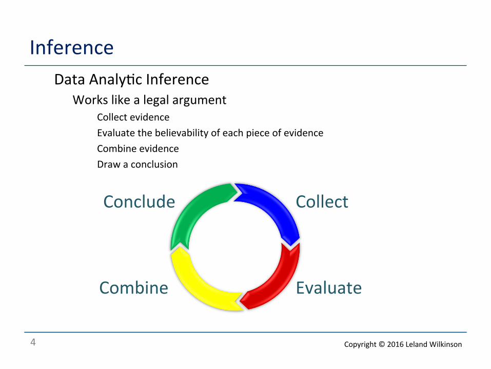
Inference o Data Analy<c Inference
o Works like a legal argument o Collect evidence o Evaluate the believability of each piece of evidence o Combine evidence o Draw a conclusion
Conclude Collect
Combine Evaluate
Copyright © 2016 Leland Wilkinson
5
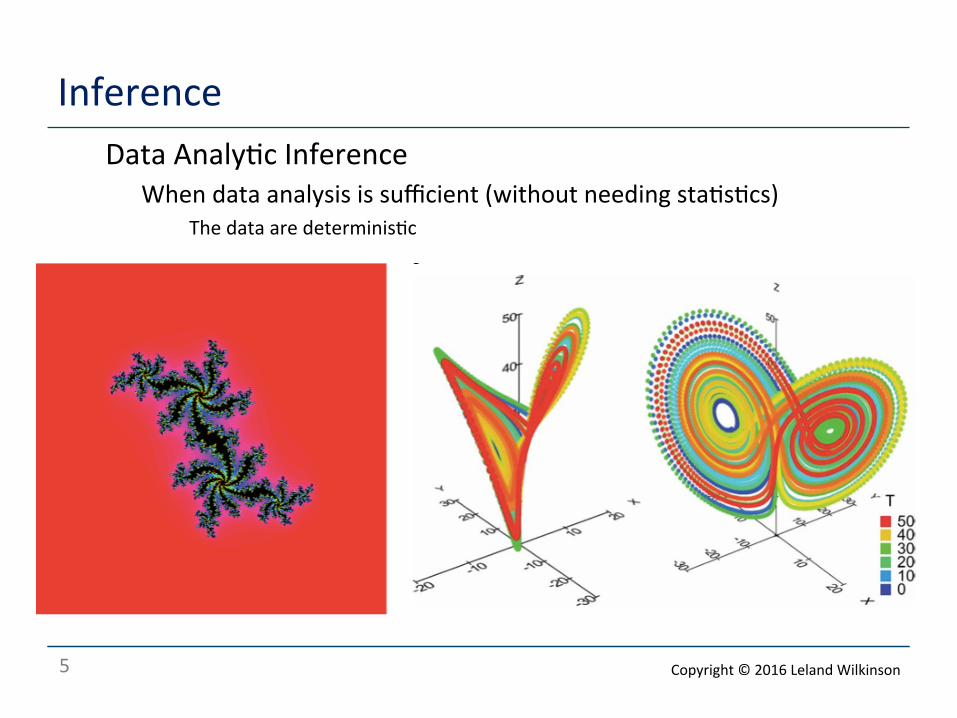
Inference o Data Analy<c Inference
o When data analysis is sufficient (without needing sta<s<cs) o The data are determinis<c
Copyright © 2016 Leland Wilkinson
6
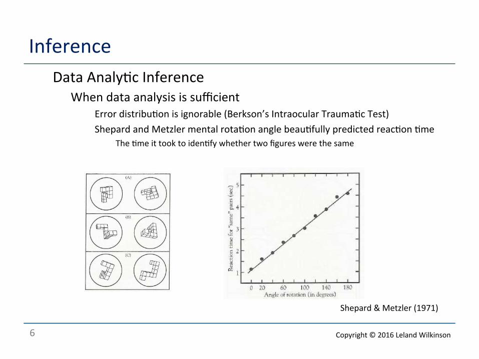
Inference o Data Analy<c Inference
o When data analysis is sufficient o Error distribu<on is ignorable (Berkson’s Intraocular Trauma<c Test) o Shepard and Metzler mental rota<on angle beau<fully predicted reac<on <me
o The <me it took to iden<fy whether two figures were the same
Shepard & Metzler (1971)
Copyright © 2016 Leland Wilkinson
7
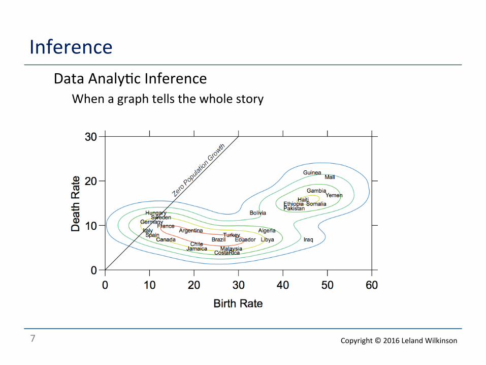
Inference o Data Analy<c Inference
o When a graph tells the whole story
Copyright © 2016 Leland Wilkinson
8
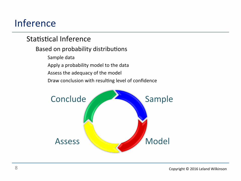
Inference o Sta<s<cal Inference
o Based on probability distribu<ons o Sample data o Apply a probability model to the data o Assess the adequacy of the model o Draw conclusion with resul<ng level of confidence
Conclude Sample
Assess Model
Copyright © 2016 Leland Wilkinson
9
Inference o Inferring Parameters of a Distribu<on via Maximum Likelihood
o We have a sample o We know (assume) it is a simple random sample (SRS) from a popula<on
o SRS: every possible sample of size n has an equal probability of being selected o Each observa<on sampled is independent of the others sampled o We know (assume) the probability distribu<on represen<ng the popula<on
o What is not a random sample? o Every other case, record, instance, number in the phone book, etc. o First n cases o Any method that fails to consider every possible case o Persi Diaconis tossing a coin (he can toss heads every <me) o Human-‐generated random numbers (people can’t imitate randomness) o Pseudo-‐random numbers
o Actually, good algorithms produce numbers indis<nguishable from truly random o So we use them and hold our breath
Copyright © 2016 Leland Wilkinson
10
Inference o Inferring Parameters of a Distribu<on via Maximum Likelihood
o How do we infer the parameter(s) of that probability distribu<on? o The likelihood that is our parameter value, based on our sample informa<on is:
o The likelihood is the probability of observing our sample values based on different values of o It is not a probability density func<on (its mass or the area under it is not 1)
o We are going to maximize this likelihood in order to es<mate o Because we want our es<mate to be the most likely value to have generated our data
θL(θ;x1, . . . , xn) = P (x1, . . . , xn; θ)
θ
θ
Copyright © 2016 Leland Wilkinson
11
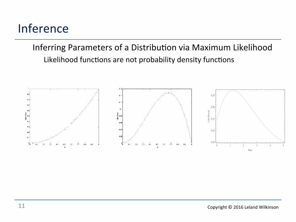
Inference o Inferring Parameters of a Distribu<on via Maximum Likelihood
o Likelihood func<ons are not probability density func<ons
Copyright © 2016 Leland Wilkinson
12
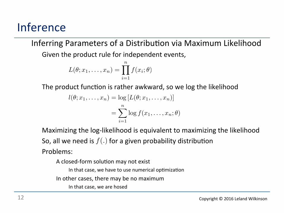
Inference o Inferring Parameters of a Distribu<on via Maximum Likelihood
o Given the product rule for independent events,
o The product func<on is rather awkward, so we log the likelihood
o Maximizing the log-‐likelihood is equivalent to maximizing the likelihood o So, all we need is for a given probability distribu<on o Problems:
o A closed-‐form solu<on may not exist o In that case, we have to use numerical op<miza<on
o In other cases, there may be no maximum o In that case, we are hosed
L(θ;x1, . . . , xn) =n�
i=1
f(xi; θ)
f(.)
l(θ;x1, . . . , xn) = log [L(θ;x1, . . . , xn)]
=n�
i=1
log f(x1, . . . , xn; θ)
Copyright © 2016 Leland Wilkinson
13
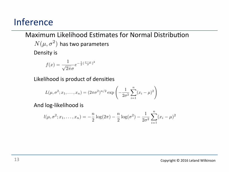
Inference o Maximum Likelihood Es<mates for Normal Distribu<on
o has two parameters o Density is
o Likelihood is product of densi<es
o And log-‐likelihood is
N(µ,σ2)
f(x) =1√2πσ
e−12 (
x−µσ )2
l(µ,σ2;x1, . . . , xn) = −n
2log(2π)− n
2log(σ2)− 1
2σ2
n�
i=1
(xi − µ)2
L(µ,σ2;x1, . . . , xn) = (2πσ2)n/2 exp
�− 1
2σ2
n�
i=1
(xi − µ)2�
Copyright © 2016 Leland Wilkinson
14
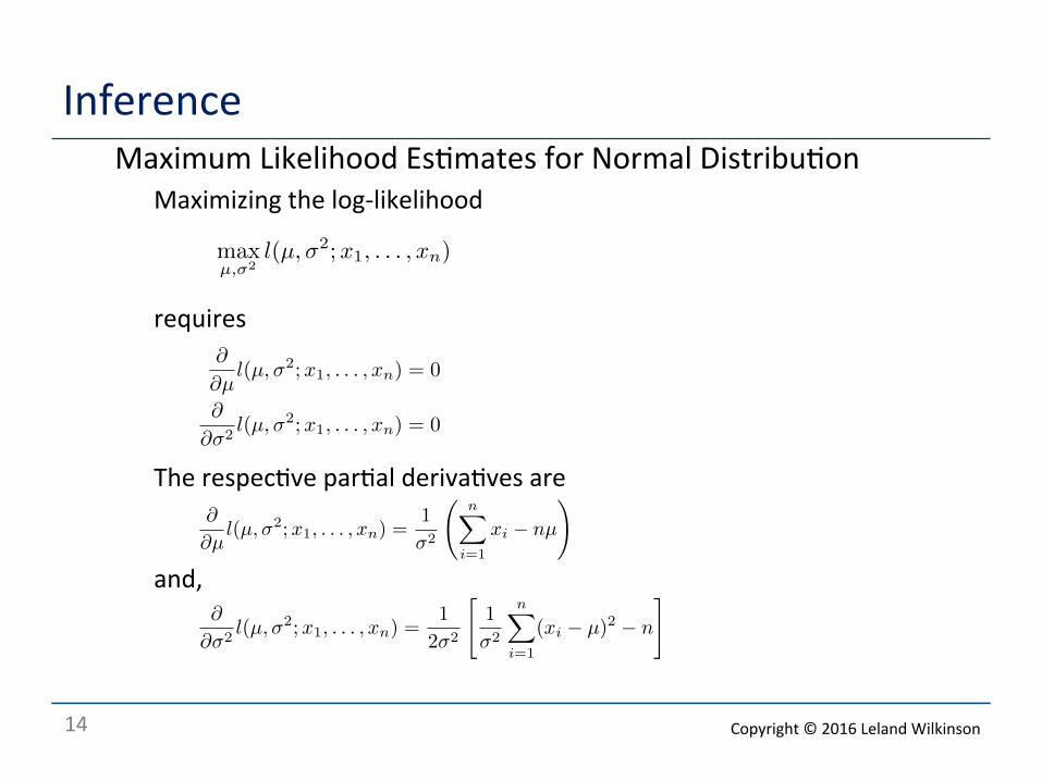
Inference o Maximum Likelihood Es<mates for Normal Distribu<on
o Maximizing the log-‐likelihood
o requires
o The respec<ve par<al deriva<ves are
o and,
maxµ,σ2
l(µ,σ2;x1, . . . , xn)
∂
∂µl(µ,σ2;x1, . . . , xn) = 0
∂
∂σ2l(µ,σ2;x1, . . . , xn) = 0
∂
∂µl(µ,σ2;x1, . . . , xn) =
1
σ2
�n�
i=1
xi − nµ
�
∂
∂σ2l(µ,σ2;x1, . . . , xn) =
1
2σ2
�1
σ2
n�
i=1
(xi − µ)2 − n
�
Copyright © 2016 Leland Wilkinson
15
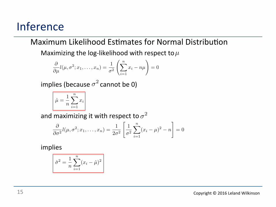
Inference o Maximum Likelihood Es<mates for Normal Distribu<on
o Maximizing the log-‐likelihood with respect to
o implies (because cannot be 0)
o and maximizing it with respect to
o implies
∂
∂µl(µ,σ2;x1, . . . , xn) =
1
σ2
�n�
i=1
xi − nµ
�= 0
∂
∂σ2l(µ,σ2;x1, . . . , xn) =
1
2σ2
�1
σ2
n�
i=1
(xi − µ)2 − n
�= 0
µ
σ2
σ2
µ̂ =1
n
n�
i=1
xi
σ̂2 =1
n
n�
i=1
(xi − µ̂)2
Copyright © 2016 Leland Wilkinson
16
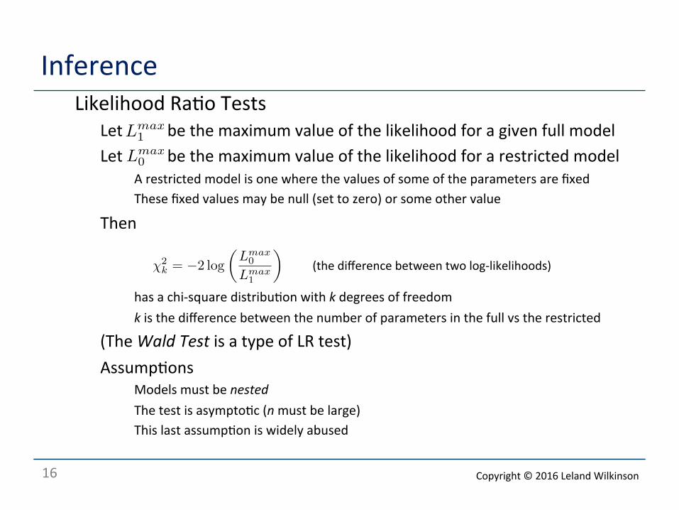
Inference o Likelihood Ra<o Tests
o Let be the maximum value of the likelihood for a given full model o Let be the maximum value of the likelihood for a restricted model
o A restricted model is one where the values of some of the parameters are fixed o These fixed values may be null (set to zero) or some other value
o Then
o has a chi-‐square distribu<on with k degrees of freedom o k is the difference between the number of parameters in the full vs the restricted
o (The Wald Test is a type of LR test) o Assump<ons
o Models must be nested o The test is asympto<c (n must be large) o This last assump<on is widely abused
Lmax0
Lmax1
χ2k = −2 log
�Lmax0
Lmax1
�(the difference between two log-‐likelihoods)
Copyright © 2016 Leland Wilkinson
17
Inference o Inferring Parameters of a Distribu<on via the Bootstrap
o Efron (1981) o Sample with replacement from a sample o Compute es<mate of a parameter from this bootstrap sample o Do this lots of <mes (say, 1000) o Histogram the bootstrap parameter es<mates o Compute sample sta<s<cs on histogram
o sample mean, sd o frac<les o confidence intervals
o Or, smooth the histogram before compu<ng sta<s<cs
o Efron and others have proofs for why this works o Not as effec<ve for skewed distribu<ons o Not as effec<ve for dependent observa<ons
Copyright © 2016 Leland Wilkinson
18
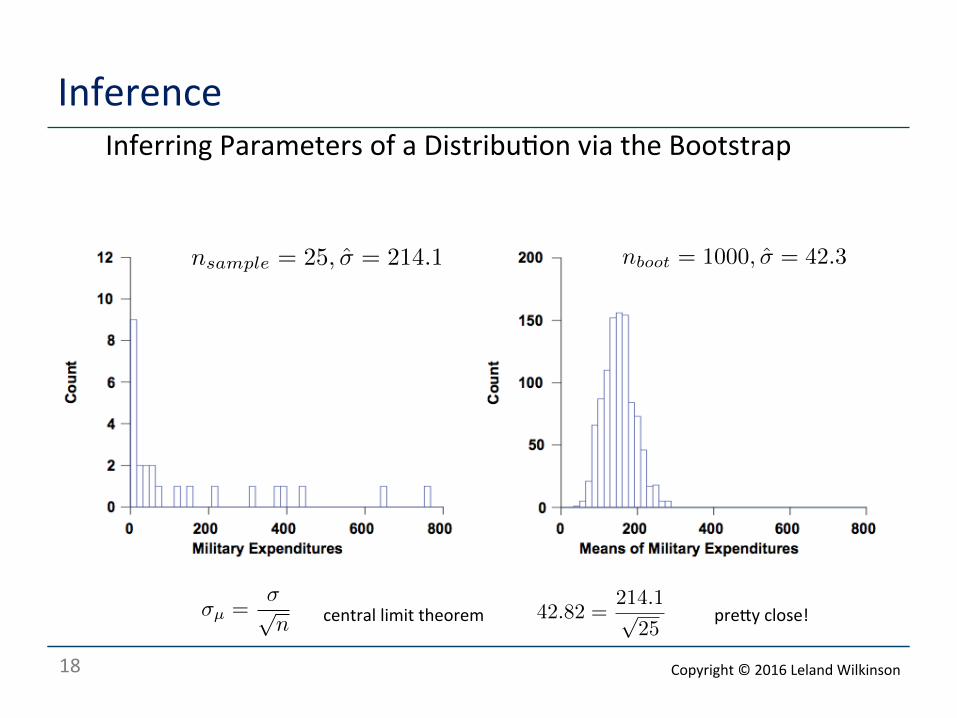
Inference o Inferring Parameters of a Distribu<on via the Bootstrap
σµ =σ√n
42.82 =214.1√
25central limit theorem preRy close!
nsample = 25, σ̂ = 214.1 nboot = 1000, σ̂ = 42.3
Copyright © 2016 Leland Wilkinson
19
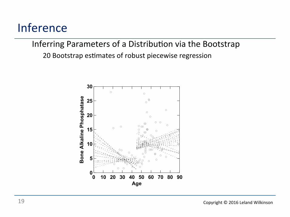
Inference o Inferring Parameters of a Distribu<on via the Bootstrap
o 20 Bootstrap es<mates of robust piecewise regression
Females
0 10 20 30 40 50 60 70 80 90Age
0
5
10
15
20
25
30B
one
Alk
alin
e Ph
osph
atas
e
Copyright © 2016 Leland Wilkinson
20
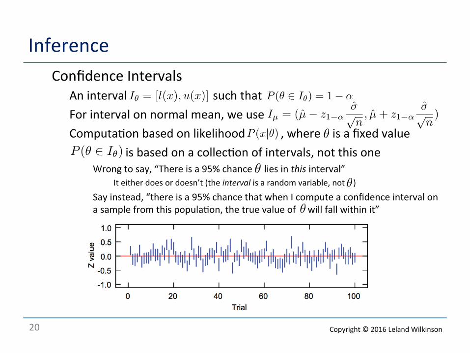
Inference o Confidence Intervals
o An interval such that o For interval on normal mean, we use o Computa<on based on likelihood , where is a fixed value o is based on a collec<on of intervals, not this one
o Wrong to say, “There is a 95% chance lies in this interval” o It either does or doesn’t (the interval is a random variable, not )
o Say instead, “there is a 95% chance that when I compute a confidence interval on a sample from this popula<on, the true value of will fall within it”
Iθ = [l(x), u(x)] P (θ ∈ Iθ) = 1− α
P (x|θ) θ
P (θ ∈ Iθ)
θ
θ
θ
Iµ = (µ̂− z1−ασ̂√n, µ̂+ z1−α
σ̂√n)
Copyright © 2016 Leland Wilkinson
21
Inference o Why confidence is not probability
o Let o There is a 25% chance that both and will lie below o There is a 25% chance that both and will lie above o Therefore, there is a 50% chance that will lie between them o Then is a 50% confidence interval o However, when , it MUST contain , even though o is a confidence interval o In other words, confidence intervals are not betworthy o Har<gan proved this argument for other distribu<ons (e.g., Normal)
o Thanks to Jerry Dallal for dis<lling Har<gan’s argument
θ
x1 x2
x1 x2
y2 − y1 > 1
(y1, y2)
θθ
(y1 = min[x1, x2], y2 = max[x1, x2])
x1, x2 ∼ U(θ − 1, θ + 1)
θ
Copyright © 2016 Leland Wilkinson
22
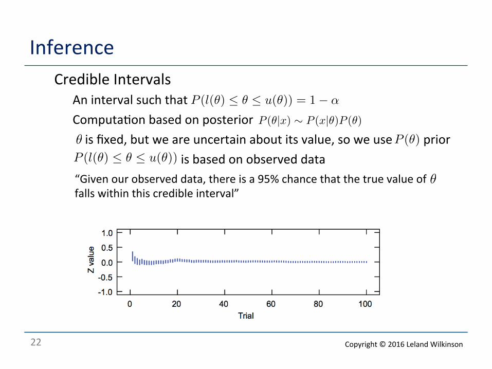
Inference o Credible Intervals
o An interval such that o Computa<on based on posterior o is fixed, but we are uncertain about its value, so we use prior o is based on observed data
P (l(θ) ≤ θ ≤ u(θ)) = 1− α
P (l(θ) ≤ θ ≤ u(θ))
θ P (θ)
“Given our observed data, there is a 95% chance that the true value of falls within this credible interval”
θ
P (θ|x) ∼ P (x|θ)P (θ)
Copyright © 2016 Leland Wilkinson
23
Inference o Hypothesis tes<ng
o Protec<ng against false posi<ves
o Construct Null Hypothesis H0 (usually, that a result is due to chance) o State rule for rejec<ng H0
o Compute likelihood of observed result under H0 o Draw a conclusion based on decision rule
Copyright © 2016 Leland Wilkinson
24
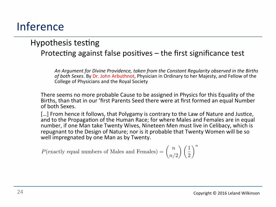
Inference o Hypothesis tes<ng
o Protec<ng against false posi<ves – the first significance test
o An Argument for Divine Providence, taken from the Constant Regularity observed in the Births of both Sexes. By Dr. John Arbuthnot, Physician in Ordinary to her Majesty, and Fellow of the College of Physicians and the Royal Society
o There seems no more probable Cause to be assigned in Physics for this Equality of the Births, than that in our ’first Parents Seed there were at first formed an equal Number of both Sexes.
o […] From hence it follows, that Polygamy is contrary to the Law of Nature and Jus<ce, and to the Propaga<on of the Human Race; for where Males and Females are in equal number, if one Man take Twenty Wives, Nineteen Men must live in Celibacy, which is repugnant to the Design of Nature; nor is it probable that Twenty Women will be so well impregnated by one Man as by Twenty.
P (exactly equal numbers of Males and Females) =
�n
n/2
��1
2
�n
Copyright © 2016 Leland Wilkinson
25
Inference o Hypothesis tes<ng
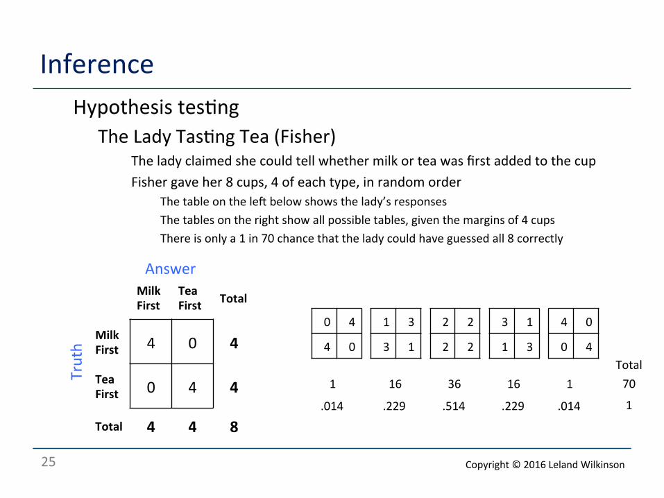
o The Lady Tas<ng Tea (Fisher) o The lady claimed she could tell whether milk or tea was first added to the cup o Fisher gave her 8 cups, 4 of each type, in random order
o The table on the les below shows the lady’s responses o The tables on the right show all possible tables, given the margins of 4 cups o There is only a 1 in 70 chance that the lady could have guessed all 8 correctly
0 4
4 0
1 3
3 1
2 2
2 2
3 1
1 3
4 0
0 4
1 16 36 1 16
.014 .229 .514 .014 .229
Milk First
Tea First Total
Milk First 4 0 4
Tea First 0 4 4
Total 4 4 8
Truth
Answer
Total 70
1
Copyright © 2016 Leland Wilkinson
26
Inference o Hypothesis tes<ng
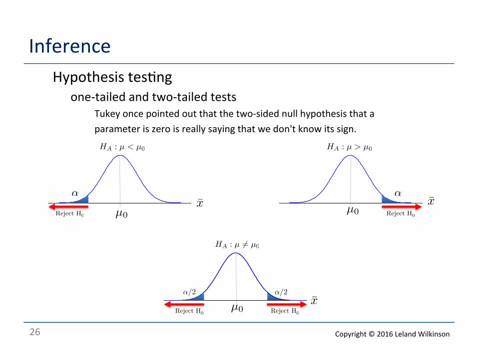
o one-‐tailed and two-‐tailed tests o Tukey once pointed out that the two-‐sided null hypothesis that a o parameter is zero is really saying that we don't know its sign.
-3 -2 -1 0 1 2 3x
0.0
0.1
0.2
0.3
0.4
f(x)
x̄α
Reject H0µ0
HA : µ > µ0
-3-2-10123x
0.0
0.1
0.2
0.3
0.4
f(x)
Reject H0
αx̄
µ0
HA : µ < µ0
-3 -2 -1 0 1 2 3x
0.0
0.1
0.2
0.3
0.4
f(x)
Reject H0 Reject H0
x̄α/2α/2
HA : µ �= µ0
µ0
Copyright © 2016 Leland Wilkinson
27
A one-‐sided test
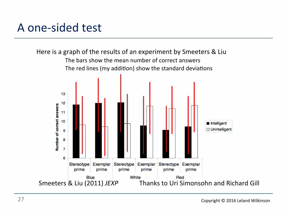
Smeeters & Liu (2011) JEXP Thanks to Uri Simonsohn and Richard Gill
Here is a graph of the results of an experiment by Smeeters & Liu The bars show the mean number of correct answers The red lines (my addi<on) show the standard devia<ons
Copyright © 2016 Leland Wilkinson
28
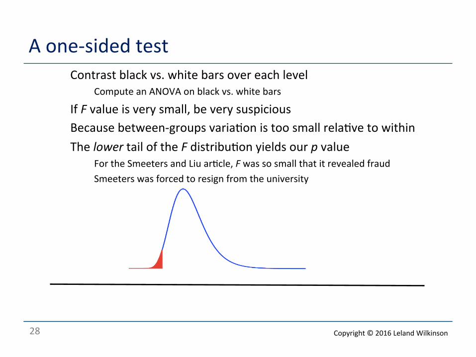
A one-‐sided test o Contrast black vs. white bars over each level
o Compute an ANOVA on black vs. white bars
o If F value is very small, be very suspicious o Because between-‐groups varia<on is too small rela<ve to within o The lower tail of the F distribu<on yields our p value
o For the Smeeters and Liu ar<cle, F was so small that it revealed fraud o Smeeters was forced to resign from the university
Copyright © 2016 Leland Wilkinson
29
Inference o Hypothesis tes<ng
o Neyman-‐Pearson procedure (Jerzy Neyman and Egon Pearson) o Construct Null Hypothesis H0 (ordinarily, that a sample result is due to chance) o Construct Alternate Hypothesis HA (ordinarily, that a sample result is not H0) o State criterion for rejec<ng H0
o Compute test sta<s<c o Make a decision based on test sta<s<c o Like Fisher’s method, this is a falsifica<on procedure o But it allows us to determine the power of the test
Copyright © 2016 Leland Wilkinson
30
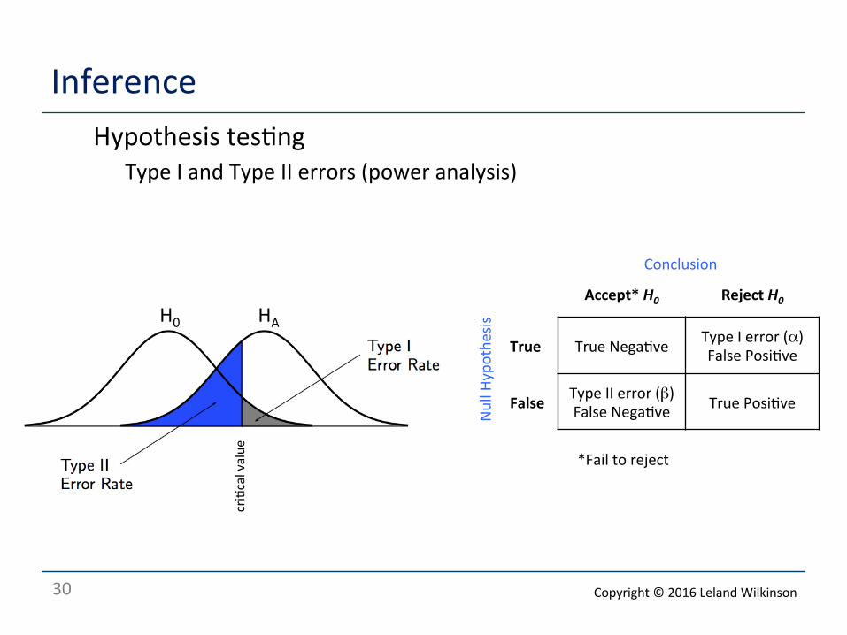
Inference o Hypothesis tes<ng
o Type I and Type II errors (power analysis)
Accept* H0 Reject H0
True True Nega<ve Type I error (α) False Posi<ve
False Type II error (β) False Nega<ve True Posi<ve
Null H
ypothe
sis
Conclusion
*Fail to reject
H0 HA
cri<cal value
Copyright © 2016 Leland Wilkinson
31
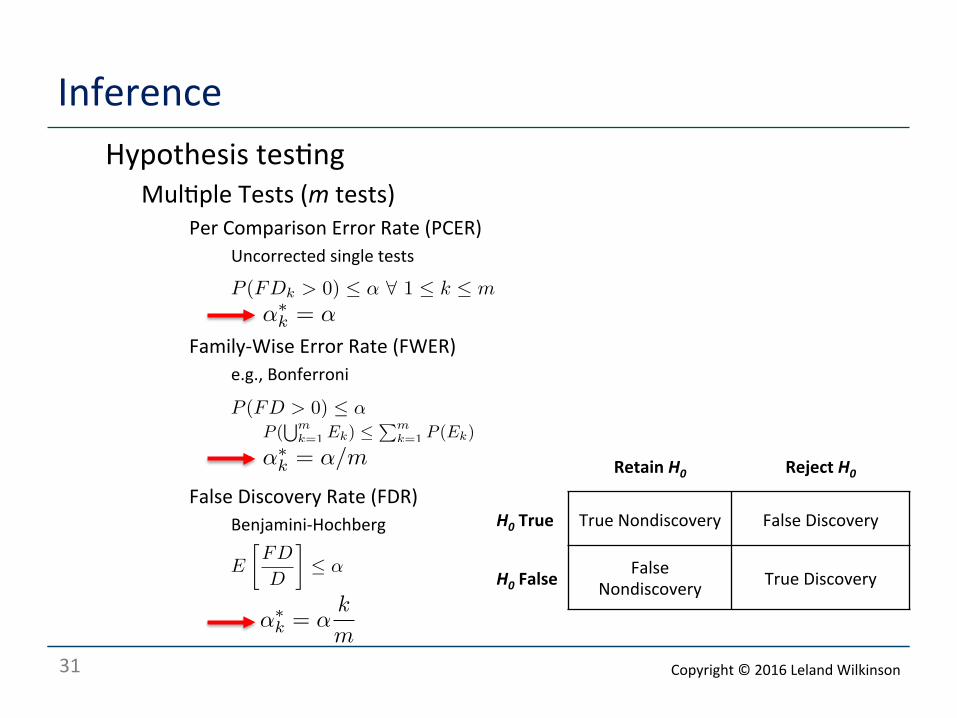
Inference o Hypothesis tes<ng
o Mul<ple Tests (m tests) o Per Comparison Error Rate (PCER)
o Uncorrected single tests
o Family-‐Wise Error Rate (FWER) o e.g., Bonferroni
o False Discovery Rate (FDR) o Benjamini-‐Hochberg
Retain H0 Reject H0
H0 True True Nondiscovery False Discovery
H0 False False
Nondiscovery True Discovery
P (FD > 0) ≤ α
E
�FD
D
�≤ α
P (FDk > 0) ≤ α ∀ 1 ≤ k ≤ m
α∗k = α
P (�m
k=1 Ek) ≤�m
k=1 P (Ek)
α∗k = α/m
α∗k = α
k
m
Copyright © 2016 Leland Wilkinson
32
Inference o Hypothesis tes<ng
o Mul<ple Tests o False Discovery Rate (FDR)
o 4 false discoveries out of 10 rejected null hypotheses is a more serious error than o 20 false discoveries out of 100 rejected null hypotheses
o Assump<on is that tests are independent o Although, this can be relaxed somewhat
o Doesn’t depend on distribu<on, only p values from tests
Copyright © 2016 Leland Wilkinson
33
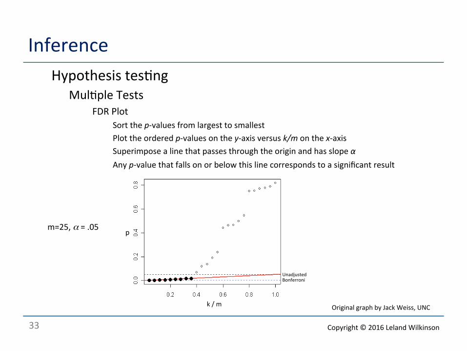
Inference o Hypothesis tes<ng
o Mul<ple Tests o FDR Plot
o Sort the p-‐values from largest to smallest o Plot the ordered p-‐values on the y-‐axis versus k/m on the x-‐axis o Superimpose a line that passes through the origin and has slope α o Any p-‐value that falls on or below this line corresponds to a significant result
Bonferroni Unadjusted
p
k / m
m=25, α = .05
Original graph by Jack Weiss, UNC
Copyright © 2016 Leland Wilkinson
34
Inference o Hypothesis tes<ng
o Covert mul<ple tests o Texas sharpshooter fallacy
o A Texan fires some gunshots at the side of a barn o He paints a target centered on the biggest cluster of hits o He then claims to be a sharpshooter
o M. Feych<ng and M. Alhbom (1992). Magne<c fields and cancer in children residing near Swedish high-‐voltage power lines. American Journal of Epidemiology, 138, 467-‐481. • Surveyed everyone living within 300 meters of high-‐voltage power lines from 1960 through 1985. • Looked for sta<s<cally significant increases in rela<ve risk (against baseline) of over 800 illnesses. • Found that there was a significant rela<ve risk of childhood leukemia for those living near power lines. • The number of illnesses considered was so large, however, that there was high probability that the
increased risk of at least one illness would appear sta<s<cally significant by chance alone. • Subsequent studies failed to show any links between power lines and childhood leukemia.
Copyright © 2016 Leland Wilkinson
35
Inference o Hypothesis tes<ng
Highly significant p-‐value doesn’t mean effect is large or strong or influen<al
Sta<s<cal significance does not imply prac<cal significance o Prac<cal significance (importance) depends on meaning, not
chance
Copyright © 2016 Leland Wilkinson
36
Inference o Hypothesis tes<ng
o H0 doesn’t mean zero value of the parameter o H0 can involve any value
o Zero value used for “nil hypothesis” instead of “null hypothesis” o Nil hypothesis is absurd, of course
Copyright © 2016 Leland Wilkinson
37
Inference o Hypothesis tes<ng
o Failure to reject H0 doesn’t prove it o Can increase n enough to make almost any H0 false
o This is a trick used in ESP research (see Duke studies)
o WRONG: p=0.05 means "the probability of the null hypothesis not being true is 95%”
o WRONG: p = .06 means "the average effect size (d=0.04) is not different from 0.”
Copyright © 2016 Leland Wilkinson
38
Inference o Hypothesis tes<ng
o Confidence intervals are not a cure for NHST problems o They come out of same calcula<ons for NHST, although they
convey more informa<on
Copyright © 2016 Leland Wilkinson
39
Inference o Hypothesis tes<ng
o p= .05 is not sacred o Fisher thought of p values as quan<fying evidence against an
hypothesis o He picked .05 for a cutoff for most prac<cal problems
Copyright © 2016 Leland Wilkinson
40
Inference o Hypothesis tes<ng
o Falsifica<on (Popper) is wrong o We build evidence for a theory o There is no such thing as a cri<cal experiment (see Kuhn) o But a theory that cannot be falsified is suspect
o Try to disprove Freud’s Oedipus Complex o Freud wouldn’t accept any evidence to the contrary
Copyright © 2016 Leland Wilkinson
41
Inference Hypothesis tes<ng
P-‐values are not the main problem • fraud • journal selec<on bias in favor of “significant” results and against “non-‐significant”
replica<on (the winner’s curse) • Publishing p-‐values without suppor<ng informa<on (effect sizes, confidence
intervals, …) • failure to control false discovery rate in mul<ple tests • small samples (low power, Tversky and Kahneman’s “Law of Small Numbers") • large samples("more than 100,000 women diagnosed from 1988 to 2011 with DCIS”;
wow! that must make this study trustworthy) • convenience samples (“we studied depression by giving a ques<onnaire to sophomore
psychology students”) • experimenter bias (failure to use double blind and other controls when available) • cherry picking (uncontrolled model selec<on, stepwise regression, …) • promiscuous mining -‐-‐ for one of the most egregious examples, see http://googlecloudplatform.blogspot.com/2014/08/correlating-patterns-of-world-history-with-bigquery.html
Copyright © 2016 Leland Wilkinson
42
Inference Hypothesis tes<ng
P-‐values are not the main problem • pollu<on from money (covert support by tobacco, sos-‐drink, chemical, energy, food
and drug companies, …) • overly complex sta<s<cal models in place of simple alterna<ves (LISREL, HLM, BUGS, …) • misuse of sta<s<cal concepts in interpre<ng results • relying on sta<s<cal bloggers or Wikipedia for advice (the madness of crowds) • 15 minutes of fame (h-‐index, cita<ons, awards, keynotes, TED talks, and other factors
driving excess publica<ons, premature media publicity, and inaRen<on to detail) • infla<on in tenure requirements (10 publica<ons a year? Are you kidding?) • pressure to get grants • ignorant media reporters (failure to understand the basics of causa<on, probability and
inference -‐-‐ coffee causes cancer, cancer causes coffee) • plagiarism (copy someone else’s study without understanding the sta<s<cs and data
analysis)
Copyright © 2016 Leland Wilkinson
43
Inference o The Bayesian objec<on
o Likelihood principle (Leonard Jimmie Savage) o Aser x is observed, all relevant experimental informa<on is contained in the
likelihood func<on for the observed x. Furthermore, two likelihood func<ons contain the same informa<on about θ if they are propor<onal to each other.
o Suppose X is the number of heads in 12 flips of a fair coin and Y is the number of flips needed to get 3 heads. o A frequen<st tests the result that X = 3 against a Binomial, with resul<ng p = .073. o But she tests the result that Y = 12 against a Nega<ve Binomial, with p = .0327. o The data are the same in both circumstances, but the experiments differ
o The difference between observing X = 3 and observing Y = 12 lies not in the actual data, but merely in the design of the experiment. In the first case, one has decided in advance to try 12 flips. In the second, one has decided to keep flipping un<l 3 successes are observed. Bayesians say the inference about θ should be the same because the two likelihoods are propor<onal to each other.
L(θ) ∝ p3(1− p)9
Copyright © 2016 Leland Wilkinson
44
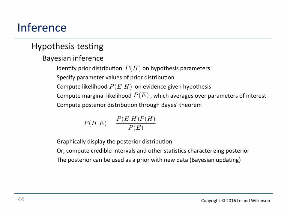
Inference o Hypothesis tes<ng
o Bayesian inference o Iden<fy prior distribu<on on hypothesis parameters o Specify parameter values of prior distribu<on o Compute likelihood on evidence given hypothesis o Compute marginal likelihood , which averages over parameters of interest o Compute posterior distribu<on through Bayes’ theorem
o Graphically display the posterior distribu<on o Or, compute credible intervals and other sta<s<cs characterizing posterior o The posterior can be used as a prior with new data (Bayesian upda<ng)
P (H)
P (E|H)P (E)
P (H|E) =P (E|H)P (H)
P (E)
Copyright © 2016 Leland Wilkinson
45
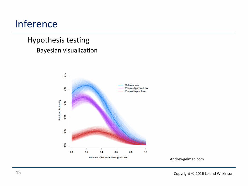
Inference o Hypothesis tes<ng
o Bayesian visualiza<on
Andrewgelman.com
Copyright © 2016 Leland Wilkinson
46
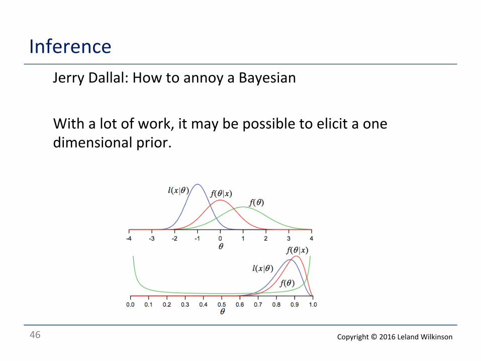
Inference o Jerry Dallal: How to annoy a Bayesian
o With a lot of work, it may be possible to elicit a one dimensional prior.
Copyright © 2016 Leland Wilkinson
47
Inference o Jerry Dallal: How to annoy a Bayesian
o With a lot of work, it may be possible to elicit a one dimensional prior.
o There may be some circumstances where, with a WHOLE lot of work, it is possible to elicit a two-‐dimensional prior.
Copyright © 2016 Leland Wilkinson
48
Inference o Jerry Dallal: How to annoy a Bayesian
o With a lot of work, it may be possible to elicit a one dimensional prior.
o There may be some circumstances where, with a WHOLE lot of work, it is possible to elicit a two-‐dimensional prior.
o NO ONE can specify a three-‐dimensional prior!
o Persi Diaconis: o It’s very hard to put meaningful priors on high-‐dimensional
real problems. And the choices can really make a difference.
Copyright © 2016 Leland Wilkinson
49
Inference o Jerry Dallal: How to annoy a Bayesian
o Even if one were to assume that a mul<variate normal distribu<on were appropriate, not only are there means and standard devia<ons to es<mate, but there are also correla<ons (or covariances) to es<mate.
o Elici<ng opinions about covariances is likely to be much more difficult that elici<ng opinions about means and standard devia<ons, and the actual values maRer…a lot!
Copyright © 2016 Leland Wilkinson
50
Inference o Jerry Dallal: How to annoy a Bayesian
o If the prior is sharp rela<ve to the likelihood, the posterior distribu<on will look like the prior.
o If the likelihood is sharp rela<ve to the prior, the posterior distribu<on will look like the likelihood.
o If neither the prior nor the likelihood is sharp rela<ve to the other, the posterior distribu<on will be a mix of the two.
Copyright © 2016 Leland Wilkinson
51
Inference o Jerry Dallal: How to annoy a Bayesian
o If the prior is sharp rela<ve to the likelihood, the posterior distribu<on will look like the prior.
o Why are we doing this study?
Copyright © 2016 Leland Wilkinson
52
Inference o Jerry Dallal: How to annoy a Bayesian
o If the likelihood is sharp rela<ve to the prior, the posterior distribu<on will look like the likelihood.
…and the results will be the same as from a frequenRst analysis!
This is scary. It says that frequenRst results that could be mistaken for probability statements really are probability statements!
Copyright © 2016 Leland Wilkinson
53
Inference o Jerry Dallal: How to annoy a Bayesian
o If neither the prior nor the likelihood is sharp rela<ve to the other, the posterior distribu<on will be a mix of the two.
Be afraid! Be very afraid!! (See next slide…)
Copyright © 2016 Leland Wilkinson
54
Inference o Jerry Dallal: How to annoy a Bayesian
o Whose prior? o Sponsors o Special Interest Groups* o Inves<gators o Reviewers o Policy Makers o Consumers
*If you are my friend, you will do your best to avoid using the word
“stakeholder” in my presence, says Jerry.
Copyright © 2016 Leland Wilkinson
55
Inference o Jerry Dallal: How to annoy a Bayesian
o Bayes methods do not allow for surprise! o This is by defini<on. A prior distribu<on reflects belief about
expecta<ons.
Copyright © 2016 Leland Wilkinson
56
Inference o Jerry Dallal: How to annoy a Bayesian
o Something that is impossible under the prior distribu<on MUST be impossible under the posterior distribu<on. Okay, nothing is impossible, so we'll withhold a bit of prior probability to spread around (…but how much?)
o This doesn't solve the problem. Something that is unexpected under the prior must s<ll be rare under the posterior unless there is a HUGE amount of data, or it really wasn't all that unexpected.
Copyright © 2016 Leland Wilkinson
57
Inference o Who is right?
Copyright © 2016 Leland Wilkinson
58
Inference o Who is right?
o Both o Sta<s<cal methodology is not going to sa<sfy philosophers any <me soon
o (Nobody seems to sa<sfy a philosopher)
o Frequen<st sta<s<cal procedures have proved effec<ve in prac<ce o Drug trials (including “best of breed” H0) o Frequen<sts do use Bayes’ theorem o Frequen<sts do take prior knowledge into account when they design experiments
o Especially when compu<ng power
o Bayesian procedures have brought plausibility to social science research o Frequen<st and Bayesian analyses osen come up with similar results o And when they don’t, disagreements can lead to progress
o Science is all about controversy o So is the law o So are poli<cs o So is religion o So is life o Oh, never mind…
Copyright © 2016 Leland Wilkinson
59
Inference o Problems with Frequen<st Inference
o Sir David Cox (a Frequen<st) o “… I felt, for instance, that various aspects of the Neyman-‐Pearson theory -‐-‐
choose alpha, choose a cri<cal region, reject or accept the null hypothesis -‐-‐ give a rigid procedure, that this isn't the way to do science.”
o “Neyman talked a lot about induc<ve rules of behavior and it seemed to me he took the view that the only thing that you could ever say is if you follow this procedure again and again, then 95% of the <me something will happen; that you couldn't say anything about a par<cular instance. Now, I don't think that's how he actually used sta<s<cal methods when it came to applica<ons; he took a much more flexible way.
o But even apart from that, you can say, is this no<on of 5% or 95% region -‐-‐ is this just an explana<on of what a 95% confidence interval would mean? A sort of hypothe<cal explana<on, if you were to do so and so, such and such would happen? Or is it an instruc<on on how to do science? It seems to me okay as the first, in fact very good as the first, terrible as the second.”
Copyright © 2016 Leland Wilkinson
60
Inference o Problems with Bayesian inference
o John Har<gan (a Bayesian)
o “The degree to which I am a Bayesian is directly propor<onal to the distance I am from the computer center.”
o “Most Bayesians reject frequen<st ideas as being outrageous and the next thing that comes out of their mouths is, ‘Let’s use these Bayesian techniques that match up with frequen<st methods.’ Therefore, although they object to frequen<st philosophy, they follow frequen<st prac<ce.”
Copyright © 2016 Leland Wilkinson
61
Inference o Inference is worthless without data analysis
o No experiment in the real world has i.i.d. trials o Small random samples do not insure ceteris paribus o Matching (blocking) doesn’t either o Experiments in the real world are difficult to replicate o All data are contaminated
o Mixtures o Outliers
o Distribu<ons change over <me o Models are sensi<ve (even robust models) o Time/space dependencies are more harmful than outliers o There are no good tests of distribu<onal shape
o Tests for normality are dubious; don’t waste your <me o Tests for mul<normality are worthless o There is no subs<tute for looking at your data
o But ignore the rules of inference and Nature will bite you Copyright © 2016 Leland Wilkinson
62
Inference o References
o Barry, Daniel (2005). A Conversation with John Hartigan. Statistical Science, 20(4), 418–430.
o Hacking, Ian (1965). Logic of Statistical Inference. Cambridge: Cambridge University Press.
o Hawkins, D. (1980). Identification of Outliers. New York: Chapman and Hall. o Ioannidis, J.P. (2005). Why most published research findings are false. PLoS Medicine. o Reid, Nancy (1994). A Conversation with Sir David Cox. Statistical Science, 9(3),
439-455. o Rousseeuw, P.J., and Leroy, A.M. (1987). Robust Regression and Outlier Detection. New
York: John Wiley & Sons. o Stigler, Stephen (1986). The History of Statistics: The Measurement of Uncertainty
before 1900. Cambridge, MA: Harvard University Press. o Wilkinson, L. & Task Force on Statistical Inference, APA Board of Scientific Affairs.
(1999). Statistical methods in psychology journals: Guidelines and explanations. American Psychologist, 54(8), 594604.
Copyright © 2016 Leland Wilkinson