1

Data collection and analysis

Jørn Vatn

NTNU

2

Objectives data collection and analysis

Collection and analysis of safety and reliability data is an important element of safety management and continuous improvement

There are several aspects of utilizing experience data and we will in the following focus on

1. Learning from experience

2. Identification of common problems “Top ten”-lists (visualized by Pareto diagrams)

3. A basis for estimation of reliability parameters MTTF, MDT, aging parameters

3

Collection of data

We differentiate between Accident and incident reporting systems

These data is event-based, i.e. we report into the system only when critical events occur

Examples of such system is Synergy, and Tripod Delta Databases with the aim of estimating reliability parameters

These databases contains system description, failure events, and maintenance activities

The Offshore Reliability Data (OREDA) is one such database Such databases will be denoted RAMS databases in the following

4

RAMS data: Boundary description

A clear boundary description is imperative for collecting, merging and analyzing RAMS data from different industries, plants or sources The merging and analysis

will otherwise be based on incompatible data.

For each equipment class a boundary must be defined. The boundary defines what RAMS data are to be collected

INLET GAS CONDITIONING

STARTINGSYSTEM

DRIVERPOWER

TRANSMISSION

COMPRESSOR UNIT

1 st 2nd STAGE STAGE

INTERSTAGECONDITIONING

Recyclevalve

AFTERCOOLER

LUBRICATIONSYSTEM

CONTROL AND MONITORING

SHAFT SEALSYSTEM

MISCEL-LANEOUS

Inlet valve

Outlet valve

Coolant Power Remoteinstr.

Power Coolant

Boundary

5

RAMS Data:Equipment hierarchy

The highest level is the equipment unit class

The number of levels for subdivision will depend on the complexity of the equipment unit and the use of the data

Turnout n

Turnout 3

Turnout i

Turnout 2

Turnout 1

S w itchm echan ism

E lectrica l m otor

Hardw areclassification

Boundaryclassification

Equ

ipm

ent

cla

ssE

quip

men

tu

nit

Sub

un

itM

ain

tain

able

item

Bou

nd

ary

leve

lS

ub-b

oun

da

ryle

vel

Mai

nta

inab

leite

m le

vel

-

(Turnout containsseveral subunits)

(Switch m echanism containsseveral Maintainable item s)

6

Data categories

Equipment data Failure data Maintenance data State information

7

RAMS database structure

Inventory ..

Inventory 2

Inventory 1

Failure ..

Failure 2

Failure 1

M aintenance 3

M aintenance 2

M aintenance 1

M aintenance ...

S tate in form ation

8

Equipment data

Identification data; e.g. equipment location classification installation data equipment unit data;

Design data; e.g. manufacturer’s data design characteristics;

Application data; e.g. operation, environment

9

Equipment data (Adapted from ISO 14224) Main catego ries

Sub-categories Data

Identification Equipment location - Equipment tag number (*)

Classification - Equipment unit class e.g. (*)- Equipment type (see Annex A) (*)- - Application (see Annex A)(*)

Installation data CountryLine (from A to B)Type of line e.g. double track, high speed lineType of track e.g. main track

Equipment unit data - Equipment unit description (nomenclature)- Unique number e.g. serial number- Subunit redundancy e.g. no of redundant subunits

Design Manufacturer’s data - Manufacturer’s name (*)- Manufacturer’s model designation (*)

Design characteristics

- Relevant for each equipment class e.g. turnout radius, current feeder voltage, see Annex A (*)

Cost data

Application Operation(normal use)

- Mode while in the operating state, e.g. continuous running, standby, normally closed/open, intermittent

- Date the equipment unit was installed or date of production start-up- Surveillance period (calendar time)(*)- The accumulated operating time during the surveillance period - Number of demands during the surveillance period as applicable - Operating parameters as relevant for each equipment class e.g. number of trains passing per

hour, see Annex A

Environmental factors External environment (severe, moderate, benign)a

Remarks Additional information - Additional information in free text as applicable

10

Failure data

identification data, failure record and equipment location; failure data for characterizing a failure, e.g. failure date,

maintainable items failed, severity class, failure mode, failure cause, method of observation

11

Failure data (From ISO 14224) Cate gory Data Description

Iden tifica tion Failure record (*) Unique failure identification

Equipment location (*) Tag number

Failure date (*) Date the failure was detected (year/month/day)

Failure mode (*) At equipment unit level as well as at maintainable item level)

Impact of failure on operation

Detailed list exist

Failure data Severity class (*) Effect on equipment unit function: critical failure, non-critical failure

Failure descriptor The descriptor of the failure (see Table 18)

Failure cause The cause of the failure (see Table 19)

Subunit failed Name of subunit that failed (see examples in Annex A)

Maintainable Item(s) failed

Specify the failed maintainable item(s) (see examples in Annex A)

Method of observation How the failure was detected (see Table 20)

Re marks Additional information Give more details, if available, on the circumstances leading to the failure, additional information on failure cause etc.

12

Failure causes (Failure descriptors, From ISO 14224) No. Notation Description

1.0 Mechanical failure- general

A failure related to some mechanical defect, but where no further details are known

1.1 Leakage External and internal leakages, either liquids or gases. If the failure mode at equipment unit level is leakage, a more causal oriented failure descriptor should be used wherever possible

1.2 Vibration Abnormal vibration. If the failure mode at equipment level is vibration, a more causal oriented failure descriptor should be used wherever possible

1.3 Clearance/ alignment failure

Failure caused by faulty clearance or alignment

1.4 Deformation Distortion, bending, buckling, denting, yielding, shrinking, etc.

1.5 Looseness Disconnection, loose items

1.6 Sticking Sticking, seizure, jamming due to reasons other than deformation or clearance/alignment failures

13

Failure causes, cont

No. Notation Description

2.0 Material failure- general

A failure related to a material defect, but no further details known

2.1 Cavitation Relevant for equipment such as pumps and valves

2.2 Corrosion All types of corrosion, both wet (electrochemical) and dry (chemical)

2.3 Erosion Erosive wear

2.4 Wear Abrasive and adhesive wear, e.g. scoring, galling, scuffing, fretting, etc.

2.5 Breakage Fracture, breach, crack

2.6 Fatigue If the cause of breakage can be traced to fatigue, this code should be used

2.7 Overheating Material damage due to overheating/burning

2.8 Burst Item burst, blown, exploded, imploded, etc.

14

Failure causes, cont

No. Notation Description

3.0 Instrument failure – general

Failure related to instrumentation, but no details known

3.1 Control failure

3.2 No signal/i-ndication/ alarm

No signal/indication/alarm when expected

3.3 Faulty signal-/indication/ alarm

Signal/indication/alarm is wrong in relation to actual process. Could be spurious, intermittent, oscillating, arbitrary

3.4 Out of adjustment Calibration error, parameter drift

3.5 Software failure Faulty or no control/monitoring/operation due to software failure

3.6 Common mode failure

Several instrument items failed simultaneously, e.g. redundant fire and gas detectors

15

Failure causes, cont

No. Notation Description

4.0 Electrical failure- general

Failures related to the supply and transmission of electrical power, but where no further details are known

4.1 Short circuiting Short circuit

4.2 Open circuit Disconnection, interruption, broken wire/cable

4.3 No power/ voltage Missing or insufficient electrical power supply

4.4 Faulty power/voltage

Faulty electrical power supply, e.g. over voltage

4.5 Earth/isolation fault Earth fault, low electrical resistance

16

Failure causes, cont

No. Notation Description

5.0 External influence – general

The failure where caused by some external events or substances outside boundary, but no further details are known

5.1 Blockage/plugged Flow restricted/blocked due to fouling, contamination, icing, etc.

5.2 Contamination Contaminated fluid/gas/surface e.g. lubrication oil contaminated, gas detector head contaminated

5.3 Miscellaneous external influences

Foreign objects, impacts, environmental, influence from neighbouring systems

6.0 Miscellaneous – generala

Descriptors that do not fall into one of the categories listed above.

6.1 Unknown No information available related to the failure descriptor.

17

Maintenance data

Maintenance is carried out To correct a failure (corrective maintenance); As a planned and normally periodic action to prevent failure from

occurring (preventive maintenance).

18

Maintenance data (From ISO 14224)

Category Data Description

Identifi cation Maintenance record (*) Unique maintenance identification

Equipment location (*) Tag number

Failure record (*) Corresponding failure identification (corrective maintenance only)

Date of maintenance (*) Date when maintenance action was undertaken

Maintenance category Corrective maintenance or preventive maintenance

Maintenance activity Description of maintenance activity (see Table 21)

Impact of maintenance on operation

Zero, partial or total, (safety consequences may also be included)

Mainten ance data Subunit maintained Name of subunit maintained (see Annex A)NOTE - For corrective maintenance, the subunit maintained will normally be identical with the one specified on the failure event report

Maintainable item(s) maintained Specify the maintainable item(s) that were maintained (see Annex A)

Spare parts Spare parts required to restore the itemCost of spare parts, or links to a cost structure database..

Maintenance resources

Maintenance man-hours, per discipline

Maintenance man-hours per discipline (mechanical, electrical, instrument, others)

Maintenance man-hours, total Total maintenance man-hours.

Maintenance time Active maintenance time Time duration for active maintenance work on the equipment

Down time The time interval during which an item is in a down state

19

State information

State information (condition monitoring information) may be collected in the following manners: Readings and measurements during maintenance Observations during normal operation Continuous measurements by use of sensor technology

20

State information, discrete readings

Category Data Description

Identifi cation State information record Unique state information identification

Equipment location Tag number

Maintenance record Corresponding maintenance identification, i.e. an observation is recorded either related to corrective or preventive maintenance

Failure record Corresponding failure identification (if no maintenance is performed in relation to the failure)

Date of observation Date when state information was read

State information

Type of measurement What measurement is obtained? For example a distance measure,

Value What are the readings of the measurement?

Remarks Additional information Give more details

If the readings are taken during normal operation, there will not be a corresponding maintenance or failure record. In this case the state information is linked directly to the inventory record

21

State information, continuous readings

Category Data Description

Identifi cation State information record Unique state information identification

Equipment location Tag number

Type of measurement What measurement is obtained? For example a distance measure,

Sampling frequency What is the sampling frequency?

State information

Sensor What type of sensor is used

Data compression principle

How is data compressed, e.g. Fast Fourier Transform

Remarks Additional information Give more details

State information is linked directly to the inventory record for continuous readings

22

Data analysis

Graphical techniques Histogram Bar charts Pareto diagrams Visualization of trends

Parametric models Estimation of constant failure rate Estimation of increasing hazard rate Estimation of global trends (over the system lifecycle)

23

Pareto diagram (“Top ten”, components)

Contr

ol- and

Signa

ling Syste

m Overh

ead

line

Other

reasons -

Infras

tructu

re Break

of rai

lIrreg

ularties

by

cons

tructi

on/ r

epair

work

Telecom

m-

unica

tion

0 %

5 %

10 %

15 %

20 %

25 %

30 %

Co

ntr

ibu

tio

n t

o d

elay

tim

e [%

]

24

Presenting raw data and rates from accident and incident reporting systems

When presenting a “snapshot” of the indicators we often compare with targets value Colour codes may be used

For “occurrences” we just plot the raw data For frequencies we need to establish the “exposure”

Number of working hours in the period Number of critical work operations

25

Cross-tabulation

To see the effect of explanatory variables we could plot the number of occurrence or frequencies as a function of one or two explanatory variables

we get an indication whether the risk is unexpected high among certain groups of workers, during specific work operations, in special periods etc

26

Example of cross tabulation (dummy figures)

Onshore Offshore

ONGC employees 4 per 106 hrs 7.1 per 106 hrs

Contractors 3 per 106 hrs 2.4 per 106 hrs

Sub-contractors 8.2 per 106 hrs 12 per 106 hrs

27

Root cause analysis

The objective is to present the contributing factors to the HSE indicators

Occurrences and/or frequencies are plotted against the causation codes, see next slide

Challenges How to treat more than one causation code? Causation codes are organised in a structure

28

Causation codes in an MTO structuring

Triggering factors Underlying causes

Work organisation Work supervision Change routines Communication Working environment Requirements/procedures/guidelines

Management of company/entity Deficient safety culture Poor quality of established systems

29

HMS avvik fordelt pr. utløsende årsakerKEP 2005

0

50

100

150

200

250

300

2003 15 4 11 11 2 8 8 8 1 6 7 5 1 4

2004 262 251 124 221 163 168 169 135 97 48 79 74 48 37

2005 201 81 178 69 78 54 33 62 106 126 68 70 81 68

Iverks ikke tilstr. sikr. av arb.pl.

Unnlot å inform./varsle/komm.

Uryd. arb. pl./mangl.

renhold

Brukte utst./verkt. på feil m.

Mangelfull skilting/ avskj.

Arb.pl. var/ble

ikke tilr.

Brukte ikke korr.

pers. verne

Feilpl. gjen- stander

Mangelf. kv.kontr./ verif. av

Løse gjen- stander

Brudd på trafikk- regler

Oppf. ikke sign./tegn/

skilt

Mangelf. verneutstyr

Feil el. svikt i

utst/tekn.

HSE deviations per triggering factor

30

Trend curves, three alternatives

1. Plot number of occurrences as a function of time (histogram)

2. Plot frequencies (number/exposure) as a function of time

3. Plot both number and exposure as a function of time in the same diagram

31

HMS avvik fordelt pr. kvartalKEP 2005

0

100

200

300

400

500

600

700

0

100000

200000

300000

400000

500000

600000

700000

800000

900000

Antall registreringer 2 2 22 42 67 334 635 646 518 451 216

Arbeidstimer 270743 127600 182706 297263 523307 774040 694858 850900 769685 402764 279959

2003 1 2003 2 2003 3 2003 4 2004 1 2004 2 2004 3 2004 4 2005 1 2005 2 2005 3

Exposure (hours worked)

Incidents

Quarterly HSE deviation

32

Challenges

Difficult to see trends due to the stochastic nature of the number of events

As an alternative, plot cumulative number of events as a function of time (adjusted for exposure)

Convex plot indicates increasing risk level Concave plot indicates an improving situation The following example is based on the previous plot

33

0

0.001

0.002

0.003

0.004

0.005

0.006

2003

-1

2003

-2

2003

-3

2003

-4

2004

-1

2004

-2

2004

-3

2004

-4

2005

-1

2005

-2

2005

-3

Cumulative number of deviations

34

Interpretation of cumulative plot

A convex plot indicates an increasing frequency of incidents ()

A concave plot indicates improvement ()

35

Note

Cross-tabulation and trend curves are used to focus on safety problems, but do not indicate improvement measures

Root cause analysis identifies significant causes behind the undesired events/accidents cue on measures

Risk reducing measure should be based on an understanding of That the measure is directed against one or more failure causes (causation code) That the measure is effective in terms of e.g., cost That no negative effects of the measure is anticipated

36

Parameter estimation /bathtub curve

Time

Fai

lure

rat

e

• The bathtub curve is a basis for reliability modelling, but

• There are two such curves• The hazard rate for ”local time”• The failure intensity for ”global time”

• Combining the two:

37

Performance loss

Local time

Fai

lure

inte

nsity

/P

erfo

rman

ce lo

ss

Local time Local time

Global (system) time

1

23

4

38

Plotting techniques, lifetime data (local bath tubcurve)

Several plots exists to visualize characteristics of lifetime data TTT-plot Kaplan-Meier plot Hazard plot

All these plots assume Failure times are identical,

and independent distributes I.e. no change over

system lifetime

Examples of how life timesare generated are shown to the right

1

2

3

4

5

6

7

T 1

T 2

T 3

T 4

T 5*

T 6

T 7

t=0 End

39

TTT- Total Time on Test plot

Let T1,T2,T3,..,Tn be the recorded lifetimes

Let T(1),T(2),T(3),.. be ordered lifetimes, i.e. T(1) T(2)T(3).. Define the total test on time at time t by

where i is such that T(i) t < T(i+1)

The TTT-plot is obtained by plotting for i = 1,..,n:

ti-n+T = tTTT j

i

1=j

)()( )(

)(

)(

)(

)(

TTTTTTTT

,n

i

n

i

40

Examplei T(i)

ST(i)ST(i)+(n-i)T(i) i/n TTT Transform

0 0 0 0 0 0 00.02 0.310582

1 6000.00 6000.00 66000 0.09 0.35 0.512 8000.00 14000.00 86000 0.18 0.46 0.633 12000.00 26000.00 122000 0.27 0.65 0.714 14000.00 40000.00 138000 0.36 0.74 0.785 16000.00 56000.00 152000 0.45 0.81 0.836 18000.00 74000.00 164000 0.55 0.88 0.877 19000.00 93000.00 169000 0.64 0.90 0.918 20000.00 113000.00 173000 0.73 0.93 0.949 23000.00 136000.00 182000 0.82 0.97 0.96

10 24000.00 160000.00 184000 0.91 0.98 0.9811 27000.00 187000.00 187000 1.00 1.00 1.00

41

Example plot

0

0.1

0.2

0.3

0.4

0.5

0.6

0.7

0.8

0.9

1

0 0.2 0.4 0.6 0.8 1

42

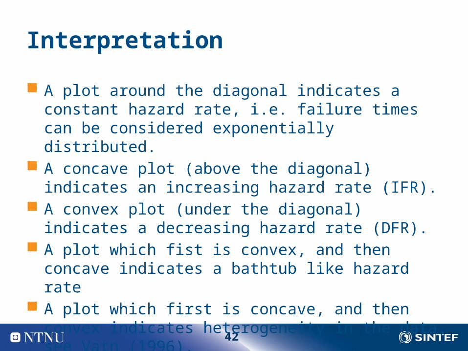
Interpretation

A plot around the diagonal indicates a constant hazard rate, i.e. failure times can be considered exponentially distributed.

A concave plot (above the diagonal) indicates an increasing hazard rate (IFR).

A convex plot (under the diagonal) indicates a decreasing hazard rate (DFR).

A plot which fist is convex, and then concave indicates a bathtub like hazard rate

A plot which first is concave, and then convex indicates heterogeneity in the data, see Vatn (1996).

43

Exercise

Assume that the following failure data for one component type has been recorded (in months)

8,9,7,6,12,18,14,6,9,11,24 Construct the TTT plot What would you say about the hazard rate?

44

The Nelson Aalen plot for global trend over the system lifetime

The Nelson-Aalen plot shows the cumulative number of failures on the Y-axis, and the X-axis represents the time

A convex plot indicates a deteriorating system, whereas a concave plot indicates an improving system

The idea behind the Nelson-Aalen plot is to plot the cumulative number of failures against time

Actually we plot W(t) which is the expected cumulative numbers of failures in a time interval

45

Nelson Aalen procedure

When estimating W(t) we need failure data from one or more processes (systems)

Each process (system) is observed in a time interval (ai,bi] and tij denotes failure time j in process i (global or calendar time)

To construct Nelson Aalen plot the following algorithm could be used Group all the tij’s and sort them, and denote the result tk, k = 1,2,…..

For each k, let Ok denote the number of processes that are under observation just before time tk

Let Let, k = 1,2,… Plot

0ˆ0 W

kkk OWW /1ˆˆ1

)ˆ,( kk Wt

46

Example of Nelson Aalen plot

ai bi tij

0 50 7, 20, 35, 44

20 60 26, 33, 41, 48, 57

40 100 50, 60, 69, 83, 88, 92, 99

0

2

4

6

8

10

12

0 10 20 30 40 50 60 70 80 90 100

47

Parameter estimation

Constant hazard rate, homogeneous sample Constant hazard rate, non-homogeneous sample Increasing hazard rate

48

Constant failure rate homogeneous sample

In this situation we only need the following information t = aggregated time in service n = the total number of observed failures in the period

An estimate for the failure rate is given by

t

n

service in timeAggregated

failures ofNumber ̂

49

Multi-Sample Problems

In many cases we do not have a homogeneous sample of data

The aggregated data for an item may come from different installations with different operational and environmental conditions, or we may wish to present an “average” failure rate estimate for slightly different items

In these situations we may decide to merge several more or less homogeneous samples, into what we call a multi-sample

The various samples may have different failure rates, and different amounts of data

50

Illustration, multi-sample dataSample

1

2

3

k

Total

Failure rate(failures per 104 hours)1 2 53 10984 6 7 11 12

Uncertainty limits

51

Estimation principles, multi-sample

The OREDA-estimator used in the OREDA data handbook is based on the following assumptions: We have k different samples. A sample may e.g., correspond to a

platform, and we may have data from similar items used on k different platforms.

In sample no. i we have observed ni failures during a total time in service ti, for i =1,2,…, k.

Sample no. i has a constant failure rate i, for i =1,2,…, k. Due to different operational and environmental conditions, the

failure rate i may vary between the samples. This variation is described by a probability density function, say

() The OREDA handbook presents expectation and standard

deviation in the estimated distribution of ()

52

Increasing hazard rate The estimation of parameters e.g., the Weibull distribution

requires Maximum Likelihood procedures. Let be the parameter vector of interest, for example = [,] if

the Weibull distribution is considered Let tj denote the observed life times, both censored and real life

times The likelihood function is now given by

where CL, U and CR are the set of left-censored (start of observation not known, uncensored (real lifetimes) and right-censored life times (failure time not known)

The estimator is the value of that maximizes L(;t)

RL Cj

jUj

jCj

j tRtftFL );();();();( θθθtθ

53

How to do it?

Usually we use numerical methods to maximize the likelihood function

Such a procedure is implemented in the TTTPlot.xls file

For the example data we get

a3.05630302

l 0.000052

54

Exercise

Assume that the following failure data for one component type has been recorded (in months)

8,9,7,6,12,18,14,6,9,11,24 Find the ML estimators for the parameters in the Weibull

distribution Compare the parametric plot (Weibull) with the TTT plot,

and judge how well the data fit the Weibull distribution

55

Likelihood function, Weibull model

Assume t(1), t(2),…t(n) are ordered failure times, and I(1), I(2),…I(n)

are indicators such that I(i) = 1 if failure time (i) is a failure time, and 0 if it is a censoring life time.

The probability density function is given by

The survival function is given by

The log likelihood function is given by

56

Exercise

Assume that the following failure data for one component type has been recorded (in months)

8,9,7,6,12,18,14,18*,6,9,11,24,30*,28* Find the ML estimators for the parameters in the Weibull

distribution where failure times with a star (*) represent censoring failure times

57

Kaplan Meier estimator

The standard TTT plot assumes that we do not have censoring failure times

The Kaplan Meier estimator and corresponding plot may be used for censoring life times

Let t(1), t(2),…t(n) be ordered failure times with corresponding indicator variable to indicate the real failure times

Let n(i) be the number of components “at risk” just prior to t(i) and s(i) the number of “deaths” at that time

The Kaplan Meier estimator is given by:

58

Exercise

Assume that the following failure data for one component type has been recorded (in months)

8,9,7,6,12,18,14,18*,6,9,11,24,30*,28* Construct the Kaplan Meier plot, and insert a Weibull

distribution overlay curve with the parameters estimated

59

Estimation in NHPP

The Non-Homogeneous Poison Process (NHPP) is a model defined by: A system is put into service at time t = 0. If the system fails, a repair is conducted and the system is put into

service after a time that could be neglected The repair action set the system back to a state as good as it was

immediately prior to the failure, i.e. a minimal repair.

The important parameter is w(t) = ROCOF = Probability of failure in (t, t + t) divided by t

60

For the NHPP we have The rate of occurrence of failures, ROCOF = w(t) is

generally not constant. The number of failures in an interval (a,b) is Poisson

distributed with parameter The mean number of failures in an interval (a,b) is The cumulative number of failures up to time t is

61

Properties for selected NHPP models

Property Model Power law model

Linear model

Log-linear model

ROCOF = w(t) t-1 (1+t) e+t

W(t) t (t+t2/2) (e+t - e)/System improves for < 1 < 0 < 0

System deteriorates for > 1 > 0 > 0

Average failure rate when replaced at time

-1 (1+/2) (e+ - e)/()

62

Estimation in NHPP

A NHPP observed over a period 0 a < b We have observed n failure times t1, t2,…, tn sorted in time

The likelihood function, say L(,t), is now the probability that we have observed the actual failure times, i.e. t = [t1, t2,…, tn] as a function of

Consider small time intervals around the observed failure times and let ti be such a small time interval following ti

The likelihood function

63

This yields

Likelihood =

Log likelihood =

64

Bayesian estimation

In some situations we may have tacit knowledge in terms of expert knowledge

Experts are typically experienced people in the project organisation

By an elicitation procedure we may get the experts to state their uncertainty distribution regarding parameters of interest

This uncertainty distribution is combined by data to find the final parameter estimates

65

Procedure Specify a prior uncertainty distribution of the reliability

parameter, () Structure reliability data information into a likelihood

function, L(;x) Calculate the posterior uncertainty distribution of the

reliability parameter vector, (x) The posterior is found by (x) L(;x) (), and

the proportionality constant is found by requiring the posterior to integrate to one

The Bayes estimate for the reliability parameter is given by the posterior mean

66

Example: Constant failure rate

= failure rate treated as a random quantity Prior expert distribution from the elicitation procedure:E() = 0.710-6 (failures / hour)SD() = 0.310-6

For mathematical simplicity, a gamma prior is used with parameters and where E = / and Var = / 2 = E/SD2 = (0.710-6)/( 0.310-6)2 = 7.78106 = E = (7.78106) (0.710-6) = 5.44

67

Example, cont

Data:t = total time in service, = 525 600 hours (e.g. 60 detector years)n = 1 = number of failures observed

Constant exponentially distributed failure times the number of failures in a period of length t, N(t), is Poisson distributed with parameter t

The probability of observing n failures is then L(;n,t) = Pr(N(t) = n) ne-t = likelihood

68

Example, cont

The posterior distribution is found by multiplying the prior distribution with the likelihood function(n) L(;n,t) () ne-t -1e- (+ n)-1e-(+t)

(+ n)-1e-(+t) is recognized as a gamma distribution with new parameters ’ =+ n, and ’ = +t

The Bayes estimate is given by the mean in this distribution, i.e.

(MLE: 1.910-6, prior mean = 0.710-6)

66

5.44 1ˆ 0.78 107.78 10 525600

n

t