data complexity in machine learning - …authors.library.caltech.edu/27081/1/dcomplex.pdfdata...

Data Complexity in Machine Learning

Ling Li and Yaser S. Abu-Mostafa

Learning Systems Group, California Institute of Technology

Abstract. We investigate the role of data complexity in the context of binary classification problems.The universal data complexity is defined for a data set as the Kolmogorov complexity of the mappingenforced by the data set. It is closely related to several existing principles used in machine learning suchas Occam’s razor, the minimum description length, and the Bayesian approach. The data complexitycan also be defined based on a learning model, which is more realistic for applications. We demonstratethe application of the data complexity in two learning problems, data decomposition and data pruning.In data decomposition, we illustrate that a data set is best approximated by its principal subsets whichare Pareto optimal with respect to the complexity and the set size. In data pruning, we show thatoutliers usually have high complexity contributions, and propose methods for estimating the complexitycontribution. Since in practice we have to approximate the ideal data complexity measures, we alsodiscuss the impact of such approximations.

1 Introduction

Machine learning is about pattern1 extraction. A typical example is an image classifier that auto-matically tells the existence of some specific object category, say cars, in an image. The classifierwould be constructed based on a training set of labeled image examples. It is relatively easy forcomputers to “memorize” all the examples, but in order for the classifier to also be able to correctlylabel images that have not been seen so far, meaningful patterns about images in general and theobject category in particular should be learned. The problem is “what kind of patterns should beextracted?”

Occam’s razor states that entities should not be multiplied beyond necessity. In other words, ifpresented with multiple hypotheses that have indifferent predictions on the training set, one shouldselect the simplest hypothesis. This preference for simpler hypotheses is actually incorporated, ex-plicitly or implicitly, in many machine learning systems (see for example Quinlan, 1986; Rissanen,1978; Vapnik, 1999). Blumer et al. (1987) showed theoretically that, under very general assump-tions, Occam’s razor produces hypotheses that can correctly predict unseen examples with highprobability. Although experimental evidence was found against the utility of Occam’s razor (Webb,1996), it is still generally believed that the bias towards simpler hypotheses is justified for real-worldproblems (Schmidhuber, 1997). Following this line, one should look for patterns that are consistentwith the examples, and simple.

But what exactly does “simple” mean? The Kolmogorov complexity (Li and Vitanyi, 1997)provides a universal measure for the “simplicity” or complexity of patterns. It says that a patternis simple if it can be generated by a short program or if it can be compressed, which essentiallymeans that the pattern has some “regularity” in it. The Kolmogorov complexity is also closelyrelated to the so-called universal probability distribution (Li and Vitanyi, 1997; Solomonoff, 2003),which is able to approximate any computable distributions. The universal distribution assigns highprobabilities to simple patterns, and thus implicitly prefers simple hypotheses.

While most research efforts integrating Occam’s razor in machine learning systems have beenfocused on the simplicity of hypotheses, the other equivalently important part in learning systems,training sets, has received much less attention in the complexity aspect, probably because training1 In a very general sense, the word “pattern” here means hypothesis, rule, or structure.

Caltech Computer Science Technical Report CaltechCSTR:2006.004, May 2006http://resolver.caltech.edu/CaltechCSTR:2006.004

2 Ling Li and Yaser S. Abu-Mostafa

sets are given instead of learned. However, except for some side information such as hints (Abu-Mostafa, 1995), the training set is the sole information source about the underlying learning prob-lem. Analyzing the complexity of the training set, as we will do in this paper, can actually revealmuch useful information about the underlying problem.

This paper is a summary of our initial work on data complexity in machine learning. We focuson binary classification problems, which are briefly introduced in Section 2. We define the datacomplexity of a training set essentially as the Kolmogorov complexity of the mapping relationshipenforced by the set. Any hypothesis that is consistent with the training set would have a programlength larger than or equal to that complexity value. The properties of the data complexity and itsrelationship to some related work are discussed in Section 3.

By studying in Section 4 the data complexity of every subset of the training set, one would findthat some subsets are Pareto optimal with respect to the complexity and the size. We call thesesubsets the principal subsets. The full training set is best approximated by the principal subsets atdifferent complexity levels, analogous to the way that a signal is best approximated by the partialsums of its Fourier series. Examples not included in a principal subset are regarded as outliersat the corresponding complexity level. Thus if the decomposition of the training set is known, alearning algorithm with a complexity budget can just train on a proper principal subset to avoidoutliers.

However, locating principal subsets is usually computationally infeasible. Thus in Section 5 wediscuss efficient ways to identify some principal subsets.

Similar to the Kolmogorov complexity, the ideal data complexity measures are either incom-putable or infeasible for practical applications. Some practical complexity measure that approxi-mates the ideal ones has to be used. Thus we also discuss the impact of such approximation to ourproposed concepts and methods. For instance, a data pruning strategy based on linear regressionis proposed in Section 5 for better robustness.

Some related work is also briefly reviewed at the end of every section. Conclusion and futurework can be found in Section 6.

2 Learning Systems

In this section, we briefly introduce some concepts and notations in machine learning, especiallyfor binary classification problems.

We assume that there exists an unknown function f , called the target function or simply thetarget, which is a deterministic mapping from the input space X to the output space Y. We focuson binary classification problems in which Y = 0, 1. An example or observation (denoted by z) isin the form of an input-output pair (x, y), where the input x is generated independently from anunknown probability distribution PX , and the output y is computed via y = f(x). A data set ortraining set is a set of examples, and is usually denoted by D = zn = (xn, yn)N

n=1 with N = |D|,the size of D.

A hypothesis is also a mapping from X to Y. For classification problems, we usually define theout-of-sample error of a hypothesis h as the expected error rate,

π(h) = Ex∼PX

Jh(x) 6= f(x)K,

where the Boolean test J·K is 1 if the condition is true and 0 otherwise. The goal of learning is tochoose a hypothesis that has a low out-of-sample error. The set of all candidate hypotheses (denotedby H) is called the learning model or hypothesis class, and usually consists of some parameterizedfunctions.

Data Complexity in Machine Learning 3

Since both the distribution PX and the target function f are unknown, the out-of-sample erroris inaccessible, and the only information we can access is often limited in the training set D. Thus,instead of looking for a hypothesis h with a low out-of-sample error, a learning algorithm may tryto find an h that minimizes the number of errors on the training set,

eD(h) =N∑

n=1

Jh(xn) 6= ynK.

A hypothesis is said to replicate or be consistent with the training set if it has zero errors on thetraining set.

However, having less errors on the training set by itself cannot guarantee a low out-of-sampleerror. For example, a lookup table that simply memorizes all the training examples has no abilityto generalize on unseen inputs. Such an overfitting situation is usually caused by endowing thelearning model with too much complexity or flexibility. Many techniques such as early stopping andregularization were proposed to avoid overfitting by carefully controlling the hypothesis complexity.

The Bayes rule states that the most probable hypothesis h given the training set D is the onethat has high likelihood Pr D | h and prior probability Pr h,

Pr h | D =Pr D | hPr h

Pr D. (1)

Having less errors on the training set makes a high likelihood, but it does not promise a high priorprobability. Regularizing the hypothesis complexity is actually an application of Occam’s razor,since we believe simple hypotheses should have high prior probabilities.

The problem of finding a generalizing hypothesis becomes harder when the examples containnoise. Due to various reasons, an example may be contaminated in the input and/or the output.When considering only binary classification problems, we take a simple view about the noise—wesay an example (x, y) is an outlier or noisy if y = 1− f(x), no matter whether the actual noise isin the input or the output.

3 Data Complexity

In this section, we investigate the complexity of a data set in the context of machine learning.The Kolmogorov complexity and related theories (Li and Vitanyi, 1997) are briefly reviewed at thebeginning, with a focus on things most relevant to machine learning. Our complexity measures for adata set are then defined, and their properties are discussed. Since the ideal complexity measures areeither incomputable or infeasible for practical applications, we also examine practical complexitymeasures that approximate the ideal ones. At the end of this section, other efforts in quantifyingthe complexity of a data set are briefly reviewed and compared.

3.1 Kolmogorov Complexity and Universal Distribution

Consider a universal Turing machine U with input alphabet 0, 1 and tape alphabet 0, 1, ,where is the blank symbol. A binary string p is a (prefix-free) program for the Turing machine Uif and only if U reads the entire string and halts. For a program p, we use |p| to denote its lengthin bits, and U(p) the output of p executed on the Turing machine U . It is possible to have an inputstring x on an auxiliary tape. In that case, the output of a program p is denoted as U(p, x).


Given a universal Turing machine U , the Kolmogorov complexity measures the algorithmiccomplexity of an arbitrary binary string s by the length of the shortest program that outputs son U . That is, the (prefix) Kolmogorov complexity KU (s) is defined as

KU (s) = min |p| : U(p) = s . (2)

KU (s) can be regarded as the length of the shortest description or encoding for the string s on theTuring machine U . Since universal Turing machines can simulate each other, the choice of U in (2)would only affect the Kolmogorov complexity by at most a constant that only depends on U . Thuswe can drop the U and denote the Kolmogorov complexity by K(s).

The conditional Kolmogorov complexity K(s | x) is defined as the length of the shortest programthat outputs s given the input string x on the auxiliary tape. That is,

K(s | x) = min |p| : U(p, x) = s . (3)

In other words, the conditional Kolmogorov complexity measures how many additional bits ofinformation are required to generate s given that x is already known. The Kolmogorov complexityis a special case of the conditional one where x is empty.

For an arbitrary binary string s, there are many programs for a Turing machine U that output s.If we assume a program p is randomly picked with probability 2−|p|, the probability that a randomprogram would output s is

PU (s) =∑

p : U(p)=s

2−|p|. (4)

The sum of PU of all binary strings is clearly bounded by 1 since no program can be the prefixof another. The U can also be dropped since the choice of U in (4) only affects the probability byno more than a constant factor independent of the string. This partly justifies why P is namedthe universal distribution. The other reason is that the universal distribution P dominates anycomputable distributions by up to a multiplicative constant, which makes P the universal prior.

The Kolmogorov complexity and the universal distribution are closely related, since we haveK(s) ≈ − log P (s) and P (s) ≈ 2−K(s). The approximation is within a constant additive or multi-plicative factor independent of s. This is intuitive since the shortest program for s gives the mostweight in (4).

The Bayes rule for learning (1) can be rewritten as

− log Pr h | D = − log Pr D | h − log Pr h+ log Pr D . (5)

The most probable hypothesis h given the training set D would minimize − log Pr h | D. Let’sassume for now a hypothesis is also an encoded binary string. With the universal prior in place,− log Pr h is roughly the code length for the hypothesis h, and − log Pr D | h is in general theminimal description length of D given h. This leads to the minimum description length (MDL)principle (Rissanen, 1978) which is a formalization of Occam’s razor: the best hypothesis for agiven data set is the one that minimizes the sum of the code length of the hypothesis and the codelength of the data set when encoded by the hypothesis.

Both the Kolmogorov complexity and the universal distribution are incomputable.

3.2 Universal Data Complexity

As we have seen, for an arbitrary string, the Kolmogorov complexity K(s) is a universal measurefor the amount of information needed to replicate s, and 2−K(s) is a universal prior probability


of s. In machine learning, we care about similar perspectives: the amount of information needed toapproximate a target function, and the prior distribution of target functions. Since a training setis usually the only information source about the target, we are thus interested in the amount ofinformation needed to replicate a training set, and the prior distribution of training sets. In short,we want a complexity measure for a training set.

Unlike the Kolmogorov complexity of a string for which the exact replication of the string ismandatory, one special essence about “replicating” a training set is that the exact values of theinputs and outputs of examples do not matter. What we really want to replicate is the input-outputrelationship enforced by the training set, since this is where the target function is involved. Theunknown input distribution PX might be important for some machine learning problems. However,given the input part of the training examples, it is also irrelevant to our task.

At first glance the conditional Kolmogorov complexity may seem suitable for measuring thecomplexity of replicating a training set. Say for D = (xn, yn)N

n=1, we collect the inputs and theoutputs of all the examples, and apply the conditional Kolmogorov complexity to the outputs giventhe inputs, i.e.,

K(y1, y2, . . . , yN | x1,x2, . . . ,xN ).

This conditional complexity, as defined in (3), finds the shortest program that takes as a wholeall the inputs and generates as a whole all the outputs. In other words, the shortest program thatmaps all the inputs to all the outputs. The target function, if encoded properly as a program, canserve the mapping with an extra loop to take care of the N inputs, as will any hypotheses that canreplicate the training set.

However, with this measure one has to assume some permutation of the examples. This is notonly undesired but also detrimental in that some “clever” permutations would ruin the purpose ofreflecting the amount of information in approximating the target. Say there are N0 examples thathave 0 as the output. With permutations that put examples having output 0 before those havingoutput 1, the shortest program would probably just encode the numbers N0 and (N − N0), andprint a string of N0 zeros and (N − N0) ones. The conditional Kolmogorov complexity would beapproximately log N0 + log(N −N0) + O(1), no matter how complicated the target might be.

Taking into consideration that the order of the examples should not play a role in the complexitymeasure, we define the data complexity as

Definition 1. Given a fixed universal Turing machine U , the data complexity of a data set D is

CU (D) = min |p| : ∀ (x, y) ∈ D, U(p,x) = y .

That is, the data complexity CU (D) is the length of the shortest program that can correctly mapevery input in the data set D to its corresponding output.

Similar to the Kolmogorov complexity, the choice of the Turing machine can only affect thedata complexity up to a constant. Formally, we have this invariance theorem.

Theorem 1. For two universal Turing machines U1 and U2, there exists a constant c that onlydepends on U1 and U2, such that for any data set D,

|CU1(D)− CU2(D)| ≤ c. (6)

Proof. Let 〈U1〉 be the encoding of U1 on U2. Any program p for U1 can be transformed to aprogram 〈U1〉 p for U2. Thus CU2(D) ≤ CU1(D) + |〈U1〉|. Let 〈U2〉 be the encoding of U2 on U1. Bysymmetry, we have CU1(D) ≤ CU2(D) + |〈U2〉|. So (6) holds for c = max |〈U1〉| , |〈U2〉|. ut


Thus the data complexity is also universal, and we can drop the U and simply write C(D).Unfortunately, the data complexity is also not a computable function.

Lemma 1. C(D) ≤ K(D) + c where c is a constant independent of D.

Proof. Let p be the shortest program that outputs D. Consider another program p′ that takesan input x, calls p to generate D on an auxiliary tape, searches x within the inputs of exampleson the auxiliary tape, and returns the corresponding output if x is found and 0 otherwise. Theprogram p′ adds a “shell” with constant length c to the program p, and c is independent of D. ThusC(D) ≤ |p′| = |p|+ c = K(D) + c. ut

Lemma 2. The data complexity C(·) is not upper bounded.

Proof. Consider any target function f : 0, 1m → 0, 1 that accepts m-bit binary strings asinputs. A data set including all possible m-bit binary inputs and their outputs from the target fwould fully decide the mapping from 0, 1m to 0, 1. Since the Kolmogorov complexity of suchmapping (for all integer m) is not upper bounded (Abu-Mostafa, 1988b,a), neither is C(·). ut

Theorem 2. The data complexity C(·) is incomputable.

Proof. We show this by contradiction. Assume there is a program p to compute C(D) for any dataset D. Consider another program p′ that accepts an integer input l, enumerates over all data sets,uses p to compute the data complexity for each data set, and stops and returns the first dataset that has complexity at least l. Due to Lemma 2, the program p′ will always halt. Denote thereturned data set as Dl. Since the program p′ together with the input l can generate Dl, we haveK(Dl) ≤ |p′|+ K(l). By Lemma 1 and the fact that C(Dl) ≥ l, we obtain l ≤ K(l) + |p′|+ c, wherec is the constant in Lemma 1. This is contradictory for l large enough since we know K(l) is upperbounded by log l plus some constant. ut

With fixed inputs, a universal prior distribution can be defined on all the possible outputs, justsimilar to the universal prior distribution. However, the details will not be discussed in this paper.

3.3 Data Complexity with Learning Models

Using our notions in machine learning, the universal data complexity is the length of the shortesthypothesis that replicates the data set, given that the learning model is the set of all programs.However, it is not common that the learning model includes all possible programs. For a limitedset of hypotheses, we can also define the data complexity.

Definition 2. Given a learning model H, the data complexity of a data set D is

CH(D) = min |h| : h ∈ H and ∀ (x, y) ∈ D, h(x) = y .

This definition is almost the same as Definition 1, except that program p has now been replaced withhypothesis h ∈ H. An implicit assumption is that there is a way to measure the “program length”or complexity of any hypothesis in the learning model. Here we assume an encoding scheme for thelearning model that maps a hypothesis to a prefix-free binary codeword. For example, the encodingscheme for feed-forward neural networks (Bishop, 1995) can be the concatenation of the number ofnetwork layers, the number of neurons in every layer, and the weights of every neuron, with eachnumber represented by a self-delimited binary string. We also assume that a program pH, calledthe interpreter for the learning model H, can take a codeword and emulate the encoded hypothesis.


Thus |h|, the complexity of the hypothesis h, is defined as the length of its codeword.2 It is easy tosee that CU (D) ≤ |pH|+ CH(D).

The data complexity as Definition 2 is in general not universal, i.e., it depends on the learningmodel and the encoding scheme, since full simulation of one learning model by another is not alwayspossible. Even with the same learning model, two encoding schemes could differ in a way that it isimpossible to bound the difference in the codeword lengths of the same hypothesis.

Definition 2 requires that some hypothesis in the learning model can replicate the data set. Thisis probably reasonable if the target is in the learning model and the data set is also noiseless. Whatif the target is not in the learning model or there is noise in the data set? A data set might not beconsistent with any of the hypotheses, and thus the data complexity is not defined for it. Actuallyin the case of noisy data sets, even if there are hypotheses that are consistent, it is not desirableto use their complexity as the data complexity. The reason will be clear later in this subsection. Insummary, we need another definition that can take care of replication errors.

Consider a hypothesis h that is consistent with all the examples except (x1, y1). We can constructa program p by memorizing input x1 with a lookup table entry:

p = if input is x1, then output y1; else run the interpreter pH on h.

Excluding the length of the interpreter, which is common to all hypotheses, the program p is just alittle longer than h, but can perfectly replicate the data set. Actually, the increase of the programlength is the length of the “if . . . then . . . else” structure plus the Kolmogorov complexity of x1

and y1. For a hypothesis that has more than one error, several lookup table entries can be used.3

If we assume the increase in the program length is a constant for every entry, we have

Definition 3. Given a learning model H and a proper positive constant λ, the data complexity(with a lookup table) of a data set D is

CH,λ(D) = min |h|+ λeD(h) : h ∈ H .

The constant λ can be seen as the equivalent complexity of implementing one lookup table entrywith the learning model. It can also be regarded as the complexity cost of one error. Definition 2does not allow any errors, so the data complexity CH(·) is actually CH,∞(·).

For positive and finite λ, the data complexity CH,λ(D) is actually computable. This is becausethe complexity is bounded by min |h| : h ∈ H+ λ |D|, and we can enumerate all codewords thatare not longer than that bound.4

Given a learning model H and an encoding scheme, which determines the hypothesis complexity,we consider a prior of hypotheses where Pr h = 2−|h|. Let’s also assume a Bernoulli noise modelwhere the probability of an example being noisy is ε. This gives the likelihood as

Pr D | h = εeD(h)(1− ε)N−eD(h) = (1− ε)N(ε−1 − 1

)−eD(h).

2 This also includes the possibility of using a universal Turing machine as the interpreter and directly mapping ahypothesis to a program. In this case, |h| is the program length.

3 There are other general ways to advise that h fails to replicate the example (x1, y1). Here is another one:

p = let y = h(input); if input is in x1, then output 1− y; else output y.

When there are several erroneous examples, x1 can be replaced with the set of the inputs of the erroneousexamples. If only very basic operations are allowed for constructing p from h, all these ways lead to the sameDefinition 3 of the data complexity.

4 Well, we also assume that every hypothesis, simulated by the interpreter, always halts. This is true for anyreasonable learning models.


And according to (5), we have

− log Pr h | D = |h|+ eD(h) · log(ε−1 − 1

)+ c,

where c = log Pr D − N log(1 − ε) is a constant independent of the hypothesis h. To maximizethe posterior probability Pr h | D or to minimize − log Pr h | D is equivalent to minimize thesum of the hypothesis complexity and the error cost for CH,λ(D), with λ = log

(ε−1 − 1

). And the

case of CH(·) or CH,∞(·) corresponds to ε = 0. The Bayesian point of view justifies the use of λ,and also emphasizes that the encoding scheme should be based on a proper prior of hypotheses.

We also have this straightforward property:

Theorem 3. CH,λ(D) ≤ CH,λ(D ∪D′) ≤ CH,λ(D) + λ |D′|.

The first inequality says that the data complexity is increasing when more examples are added. Thesecond inequality states that the increase of the complexity is at most λ |D′|, the cost of treatingall the added examples with lookup table entries. The increase would be less if some of the addedexamples can be replicated by the shortest hypothesis for D, or can form patterns which are shorterthan lookup table entries. More will be discussed on these two cases when the complexity-error pathis introduced (Definition 6 on page 19).

For the rest of the paper, we will mostly work with Definition 2 and Definition 3, and we willuse just C(·) for CH,λ(·) or CU (·) when the meaning is clear from the context. Because lookuptable entries are an integrated part of Definition 3, we will also simply use “hypothesis” to mean ahypothesis together with lookup table entries. Thus all the three data complexity definitions can beunified as the length of the shortest consistent hypothesis. We use hD to denote one of the shortesthypotheses that can replicate D.

We will also assume that any mechanisms for memorizing individual examples, no matterwhether it is built-in or implemented as lookup table entries as in Definition 3, would cost thesame complexity as a lookup table. In other words, if an example cannot help build patterns forother examples, adding it to a set would increase the data complexity by λ.

3.4 Practical Measures

Although we now have three data complexity measures, none of them is feasible in practice. The uni-versal data complexity CU (·) is incomputable. The data complexity defined on a learning model H,CH(·), may be computable for some H, but finding a hypothesis that is consistent with the dataset is usually NP-complete, not to mention finding a shortest one. The data complexity with alookup table CH,λ(·) seems the most promising to be used in practice. But it also suffers from theexponential time complexity in searching for a shortest hypothesis (with errors). We need to havesome approximate complexity measure for practical applications.

A reasonable approximation to CH(·) or CH,λ(·) can be obtained as a byproduct of the learningprocedure. A learning algorithm usually minimizes the number of errors plus some regularizationterm over the learning model, and the regularization term is usually meant to approximate thecomplexity (encoding length) of a hypothesis. Thus some information about the learned hypothesiscan be used as a practical data complexity measure. For example, the number of different literalsused to construct a mixed DNF-CNF rule was used by Gamberger and Lavrac (1997). In thefollowing text, we will deduce another practical data complexity measure based on the hard-marginsupport vector machine.

The hard-margin support vector machine (SVM) (Vapnik, 1999) is a learning algorithm thatfinds an optimal hyperplane to separate the training examples with maximal minimum margin. A


hyperplane is defined as 〈w,x〉 − b = 0, where w is the weight vector and b is the bias. Assumingthe training set is linearly separable, SVM solves the optimization problem below:

minw,b

‖w‖2 ,

subject to yn (〈w,xn〉 − b) ≥ 1, n = 1, . . . , N. (7)

The dual problem is

minα

12

N∑i=1

N∑j=1

αiαjyiyj 〈xi,xj〉 −N∑

n=1

αn,

subject to αn ≥ 0, n = 1, . . . , N,N∑

n=1

ynαn = 0.

The optimal weight vector, given the optimal α∗ for the dual problem, is a linear combination ofthe training input vectors,

w∗ =N∑

n=1

ynα∗nxn. (8)

Note that only the so-called support vectors, for which the equality in (7) is achieved, can havenonzero coefficients α∗n in (8).

For a linearly nonseparable training set, the kernel trick (Aizerman et al., 1964) is used to mapinput vectors to a high-dimensional space and an optimal separating hyperplane can be found there.Denote the inner product in the mapped space of two inputs x and x′ as K(x,x′), the so-calledkernel operation. The dual problem with the kernel trick uses the kernel operation instead of thenormal inner product, and the optimal hypothesis (a hyperplane in the mapped space but no longera hyperplane in the input space) becomes

N∑n=1

ynα∗nK(xn,x)− b∗ = 0.

Since the mapped space is usually high-dimensional or even infinite-dimensional, it is reasonableto describe the SVM hypothesis by listing the support vectors and their coefficients. Thus thedescriptive length is approximately (Mc1 + c2 + c3), where M is the number of support vectors,c1 is the average Kolmogorov complexity of describing an input vector and a coefficient, c2 is theKolmogorov complexity of the bias, and c3 is the descriptive length of the summation and thekernel operation. Since c3 is a common part for all SVM hypotheses using the same kernel, andc2 is relatively small compared to c1, we can use just the number of support vectors, M , as thecomplexity measure for SVM hypotheses.

With some minor conditions, SVM with powerful kernels such as the stump kernel and theperceptron kernel (Lin and Li, 2005a,b) can always perfectly replicate a training set. Thus themeasure based on SVM with such kernels fit well with Definition 2. In the experiments for thispaper, we used the perceptron kernel, which usually has comparable learning performance to thepopular Gaussian kernel, but do not require a parameter selection (Lin and Li, 2005b).

Note that SVM can also be trained incrementally (Cauwenberghs and Poggio, 2001). Thatis, if new examples are added after an SVM has already been learned on the training set, thehyperplane can be updated to accommodate the new examples in an efficient way. Such capabilityof incrementally computing the complexity can be quite useful in some applications, such as datapruning (Subsection 5.2) and deviation detection (Arning et al., 1996).


3.5 Related Work

Our data complexity definitions share some similarity to the randomness of decision problems.Abu-Mostafa (1988b,a) discussed decision problems where the input space of the target functionwas finite, and defined the randomness of a problem based on the Kolmogorov complexity of thetarget’s truth table. The randomness can also be based on the length of the shortest program thatimplements the target function, which is essentially equivalent to the previous definition (Abu-Mostafa, 1988a). However, in our settings, the input space is infinite and the training set includesonly finite examples; hence an entire truth table is infeasible. Thus the second way, which we haveadopted, seems to be the only reasonable definition.

Definition 3, the data complexity with a lookup table, is also similar to the two-part code lengthof the minimum description length (MDL) principle (Rissanen, 1978; Grunwald, 2005). The two-part scheme explains the data via encoding a hypothesis for the data, and then encoding the datawith the help of the hypothesis. The latter part usually takes care of the discrepancy informationbetween the hypothesis and the data, just like in Definition 3. However, in our definition, the inputsof the data are not encoded, and we explicitly ignore the order of examples when considering thediscrepancy.

The data complexity is also conceptually aligned with the CLCH value (complexity of theleast complex correct hypothesis) proposed by Gamberger and Lavrac (1997). They required thecomplexity measure for hypotheses, which is the program length in this paper, to be “reasonable.”That is, for two hypotheses, h1 and h2, where h2 is obtained by “conjunctively or disjunctivelyadding conditions” to h1, h1 should have no larger complexity than h2. However, this intuitivelycorrect requirement is actually troublesome. For instance, h1 recognizes all points in a fixed hexagon,and h2 recognizes all points in a fixed triangle enclosed in that hexagon. Although h2 can be obtainedby adding more constraints on h1, it is actually simpler than h1. Besides, their definition of a setbeing “saturated” and the corresponding “saturation test” depend heavily on the training set beinglarge enough to represent the target function, which might not be practical.

Except the usual complexity measures based on logic clauses, not many practical complexitymeasures have been studied. Schmidhuber (1997) implemented a variant of the general universalsearch (Levin, 1973) to find a neural network with a close-to-minimal Levin complexity. Althoughthe implementation is only feasible on very simple toy problems, his experiments still showed thatsuch search, favoring short hypotheses, led to excellent generalization performance, which reinforcedthe validity of Occam’s razor in learning problems.

Wolpert and Macready (1999) proposed a very interesting complexity measure called self-dissimilarity. They observed that many complex systems tend to exhibit different structural patternsover different space and time scale. Thus the degrees of self-dissimilarity between the various scaleswith which a system is examined constitute a complexity signature of that system. It is mainly acomplexity measure for a system, or a target function in our context, which can provide informationat different scales, and is not straightforward to be applied to a data set.

4 Data Decomposition

In this section, we discuss the issue of approximating a data set with its subsets. Compared withthe full data set, a subset is in general simpler (lower data complexity) but less informative (fewerexamples). In addition, different subsets can form different patterns, and thus lead to differentcombinations of the data complexity and the subset size. We show that the principal subsets,defined later in this section, have the Pareto optimal combinations and best approximate thefull set at different complexity levels. The concept of the principal subsets is also useful for datapruning (Section 5).


4.1 Complexity-Error Plots

When there is only one class of examples, the data complexity is a small constant. Only withexamples from both classes can more interesting patterns be formed. Given a training set D,different subsets of D may form different patterns, and thus lead to different complexity values.

Figure 1(a) shows a toy learning problem with a target consisting of three concentric disks. The

(a) (b) (c) (d)

Figure 1. Subsets of examples from the concentric disks problem: (a) all examples; (b) examples from the two outerrings; (c) examples within the middle disk; (d) all “×” examples

target is depicted with the “white” and “gray” backgrounds in the plot—examples on the whitebackground are classified as class 1, and examples on the gray background are classified as 0. Theexamples in the plot were randomly generated and are marked with “+” and “×” according to theirclass labels. The other three plots in Figure 1 illustrate how different subsets of the examples canbe explained by hypotheses of different complexity levels, and thus may have different complexityvalues. We also see that different subsets approximate the full set to different degrees.

For a given data set D, we are interested in all possible combinations of the data complexityand the approximation accuracy of its subsets. Consider the following set of pairs:

Ω1 = (C(S), |D| − |S|) : S ⊆ D . (9)

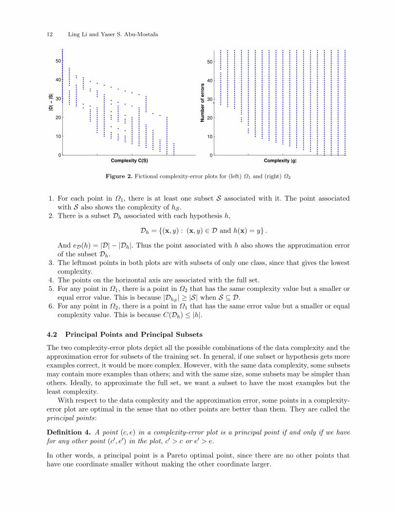
Here we use |D| − |S| as the approximation error of S.5 The set Ω1 can be regarded as a plot ofpoints on the 2-D plane. For each subset S, there is a point in Ω1 with the horizontal axis givingthe data complexity and the vertical axis showing the approximation error. Such a plot is calledthe subset-based complexity-error plot (see Figure 2).

We can also consider another set built upon programs or hypotheses:

Ω2 = (|h| , eD(h)) : h ∈ H .

This set, Ω2, has a point for each hypothesis h in the learning model, depicting the complexityof the hypothesis and the number of errors on the training set. It is called the hypothesis-basedcomplexity-error plot. Note that the hypothesis h and the learning model H shall agree with thedata complexity measure C(·) used in (9). For example, if the data complexity measure allowslookup tables, the learning model H would then includes hypotheses appended with lookup tablesof all sizes.

The two plots in Figure 2 demonstrate for a fictional training set how the two sets of pairs look.Here are some observations for the two complexity-error plots:5 If we regard S as a lookup table, the error of the lookup table on the full set is |D| − |S|.


0

10

20

30

40

50

Complexity C(S)

|D| −

|S|

0

10

20

30

40

50

Complexity |g|

Num

ber o

f err

ors

Figure 2. Fictional complexity-error plots for (left) Ω1 and (right) Ω2

1. For each point in Ω1, there is at least one subset S associated with it. The point associatedwith S also shows the complexity of hS .

2. There is a subset Dh associated with each hypothesis h,

Dh = (x, y) : (x, y) ∈ D and h(x) = y .

And eD(h) = |D| − |Dh|. Thus the point associated with h also shows the approximation errorof the subset Dh.

3. The leftmost points in both plots are with subsets of only one class, since that gives the lowestcomplexity.

4. The points on the horizontal axis are associated with the full set.5. For any point in Ω1, there is a point in Ω2 that has the same complexity value but a smaller or

equal error value. This is because |DhS | ≥ |S| when S ⊆ D.6. For any point in Ω2, there is a point in Ω1 that has the same error value but a smaller or equal

complexity value. This is because C(Dh) ≤ |h|.

4.2 Principal Points and Principal Subsets

The two complexity-error plots depict all the possible combinations of the data complexity and theapproximation error for subsets of the training set. In general, if one subset or hypothesis gets moreexamples correct, it would be more complex. However, with the same data complexity, some subsetsmay contain more examples than others; and with the same size, some subsets may be simpler thanothers. Ideally, to approximate the full set, we want a subset to have the most examples but theleast complexity.

With respect to the data complexity and the approximation error, some points in a complexity-error plot are optimal in the sense that no other points are better than them. They are called theprincipal points:

Definition 4. A point (c, e) in a complexity-error plot is a principal point if and only if we havefor any other point (c′, e′) in the plot, c′ > c or e′ > e.

In other words, a principal point is a Pareto optimal point, since there are no other points thathave one coordinate smaller without making the other coordinate larger.


Although the subset-based complexity-error plot looks quite different from the hypothesis-basedcomplexity-error plot, they actually have the same set of principal points.

Theorem 4. The subset-based and hypothesis-based complexity-error plots have the same set ofprincipal points.

Proof. The proof utilizes the observations in the previous subsection that relates points in thesetwo plots. For any principal point (c, e) ∈ Ω1, there is a point (c2, e2) ∈ Ω2 with c2 = c and e2 ≤ e.If (c2, e2) is not a principal point in Ω2, we can find a point (c′2, e

′2) ∈ Ω2 such that c′2 ≤ c2, e′2 ≤ e2,

and at least one inequality would be strict; otherwise let c′2 = c2 and e′2 = e2. For (c′2, e′2), there is

a point (c′, e′) ∈ Ω1 with c′ ≤ c′2 and e′ = e′2. Overall we have c′ ≤ c and e′ ≤ e, and either e2 < eor (c2, e2) not being a principal point will make at least one inequality be strict, which contradictsthe assumption that (c, e) is a principal point in Ω1. Thus e = e2 and (c, e) is also a principal pointin Ω2. Likewise we can also prove that any principal point of Ω2 is also a principal point in Ω1. ut

0

10

20

30

40

50

Complexity C(S)

|D| −

|S|

Figure 3. A fictional complexity-error plot with principal points circled

Figure 3 shows the principal points in the subset-based complexity-error plot from the lastfictional problem. Note that each principal point is associated with at least one subset and onehypothesis. Each principal point represents some optimal trade-off between the data complexityand the size. To increase the size of the associated subset, we have to go to a higher complexitylevel; to reduce the data complexity, we have to remove examples from the subset. Each principalpoint also represents some optimal trade-off between the hypothesis complexity and the hypothesiserror. To decrease the error on the training set, a more complex hypothesis should be sought; touse a simpler hypothesis, more errors would have to be tolerated. Thus the principal point at agiven complexity level gives the optimal error level, and implicitly the optimal subset to learn, andthe optimal hypothesis to pick.

A subset associated with a principal point is called a principal subset. The above argumentsactually say that a principal subset is a best approximation to the full set at some complexity level.


4.3 Toy Problems

We verify the use of the data complexity in data decomposition with two toy problems. The prac-tical data complexity measure is the number of support vectors in a hard-margin SVM with theperceptron kernel (see Subsection 3.4).

The first toy problem is the concentric disks problem with 31 random examples (see page 11).To have the subset-based complexity-error plot, we need to go over all the (231 − 1) subsets andcompute the data complexity for each subset. To make the job computationally more feasible, wecluster the examples as depicted in Figure 4 by examples connected with dotted lines, and onlyexamine subsets that consist of whole clusters.6 The complexity-error plot using these 15 clusters,with principal points circled, is shown in Figure 5.

Figure 4. 15 clusters of the concentric disks problem, shown as groups of examples connected with dotted lines

0 5 10 15 20 250

5

10

15

20

25

30

Number of support vectors

|D| −

|S|

Figure 5. The complexity-error plot based on the clusters of the concentric disks problem (Figure 4), with theprincipal points circled

There are 11 principal points associated with 17 principal subsets. In Figure 14 on page 30,we list all the 17 principal subsets, of which three selected ones are shown in Figure 6. The data6 The 15 clusters in Figure 4 were manually chosen based on example class and distance, such that each cluster

contains only examples of the same class, and is not too close to examples of the other class. Although this couldbe done by some carefully crafted algorithm, we did it manually since the training set is small.


(a) (0, 11) (b) (17, 3) (c) (24, 0)

Figure 6. Three selected principal subsets of the concentric disks problem (complexity-error pairs are also listed)

Figure 7. 32 clusters of the Yin-Yang problem, shown as groups of examples connected with dotted lines

complexity based on SVM-perceptron and the number of errors are also listed below the subsetplots, and the white and gray background depicts the target function. Plot (a) shows the situationwhere a simplest hypothesis predicts the negative class regardless of the actual inputs. The subsetis same as the one in Figure 1(d) on page 11. Plot (c) is the full training set with the highestdata complexity, same as the one in Figure 1(a). The middle one, plot (b) or Figure 1(b), gives anintermediate situation such that the two classes of examples in the two outer rings are replicated,but the examples in the inner disk are deserted. This implies that, at that level of complexity,examples in the inner disk should rather be regarded as outliers than exceptions to the middle disk.

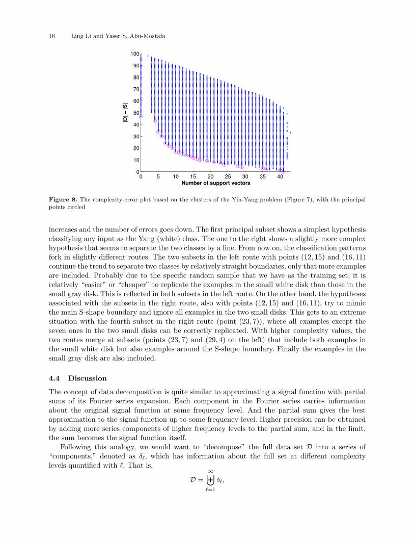
The second toy problem is about the Yin-Yang target function used by Li et al. (2005), whichis also a 2-D binary classification problem. The background colors in Figure 7 depict how the Yin-Yang target classifies examples within a round plate centered at the origin; examples out of theplate belong to the Yang (white) class if it is in the upper half-plane. The training set consistsof 100 examples randomly picked within a circle slightly larger than the plate. Clustering is alsorequired for generating the complexity-error plot. Figure 7 also shows the 32 manually chosenclusters. The resulted complexity-error plot, based on the practical data complexity measure withSVM-perceptron, is show in Figure 8.

This time we get 25 principal points and 48 associated principal sets (see Figure 15 on page 31and Figure 16 on page 32 for most of them). Here in Figure 9, we list and organize with arrows11 principal sets that we think are representative. With the flow of arrows, the data complexity


0 5 10 15 20 25 30 35 400

10

20

30

40

50

60

70

80

90

100

Number of support vectors

|D| −

|S|

Figure 8. The complexity-error plot based on the clusters of the Yin-Yang problem (Figure 7), with the principalpoints circled

increases and the number of errors goes down. The first principal subset shows a simplest hypothesisclassifying any input as the Yang (white) class. The one to the right shows a slightly more complexhypothesis that seems to separate the two classes by a line. From now on, the classification patternsfork in slightly different routes. The two subsets in the left route with points (12, 15) and (16, 11)continue the trend to separate two classes by relatively straight boundaries, only that more examplesare included. Probably due to the specific random sample that we have as the training set, it isrelatively “easier” or “cheaper” to replicate the examples in the small white disk than those in thesmall gray disk. This is reflected in both subsets in the left route. On the other hand, the hypothesesassociated with the subsets in the right route, also with points (12, 15) and (16, 11), try to mimicthe main S-shape boundary and ignore all examples in the two small disks. This gets to an extremesituation with the fourth subset in the right route (point (23, 7)), where all examples except theseven ones in the two small disks can be correctly replicated. With higher complexity values, thetwo routes merge at subsets (points (23, 7) and (29, 4) on the left) that include both examples inthe small white disk but also examples around the S-shape boundary. Finally the examples in thesmall gray disk are also included.

4.4 Discussion

The concept of data decomposition is quite similar to approximating a signal function with partialsums of its Fourier series expansion. Each component in the Fourier series carries informationabout the original signal function at some frequency level. And the partial sum gives the bestapproximation to the signal function up to some frequency level. Higher precision can be obtainedby adding more series components of higher frequency levels to the partial sum, and in the limit,the sum becomes the signal function itself.

Following this analogy, we would want to “decompose” the full data set D into a series of“components,” denoted as δ`, which has information about the full set at different complexitylevels quantified with `. That is,

D =∞⊎

`=1

δ`,


(0, 47)

→

(7, 24)

↓

(12, 15) (12, 15)

↓ ↓

(16, 11) (16, 11)

↓ ↓

(23, 7) (23, 7)

↓

(29, 4)

→

(35, 3)

→

(41, 0)

Figure 9. Eleven selected principal subsets of the Yin-Yang problem (complexity-error pairs are also listed)


where⊎

is some operation to add up the components. Although at this point we are still unclearexactly what the components δ` are and what the operation

⊎does, we would expect the partial

sum,

DL =L⊎

`=1

δ`,

which should be a subset of D, to be the best approximation to D within the complexity level L.Our analysis about the complexity-error pairs of all the subsets concludes that DL should be

a principal subset. Since a smaller principal subset is not necessarily a subset of a larger principalsubset, the decomposition component δ` is in general not a set of examples. We may consider δ`

as a set of examples that should be added and a set of examples that should be removed at thecomplexity level `.7 That is, moving from one principal subset to another generally involves addingand removing examples.

This fact also leads to the inevitable high computational complexity of locating principal subsets.It is not straightforward to generate a new principal subset from a known one, and to determinewhether a given subset is principal, exponentially many other subsets needed to be checked andcompared. This issue will be reexamined in Subsection 5.1. There we will see that the computationalcomplexity is related to the number of the complexity-error paths that contain principal points.

4.5 Related Work

A general consensus is that not all examples in a training set are equivalently important to learning.For instance, examples contaminated by noise are harmful to learning. Even in cases where all theexamples are noiseless, there are situations in which we want to deal with examples differently.For instance, in cases where none of the hypotheses can perfectly model the target, it is better todiscard examples that cannot be classified correctly by any hypothesis as they may “confuse” thelearning (Nicholson, 2002; Li et al., 2005).

There have been many different criteria to discriminate examples as different categories: con-sistent vs. inconsistent (Brodley and Friedl, 1999; Hodge and Austin, 2004), easy vs. hard (Merleret al., 2004), typical vs. informative (Guyon et al., 1996), etc. Li et al. (2005) unified some of thecriteria with the concept of intrinsic margin and group examples as typical, critical, and noisy.

The approach mentioned in this paper takes a quite different view for categorizing examples.There are no natively good or bad examples. Examples are different only because they demanddifferent amount of data complexity for describing them together with other examples. Althoughwe usually think an example is noisy if it demands too much complexity, the amount can be differentdepending on what other examples are also included in the set. Thus an example that seems noisyat some level of complexity, or with some subset of examples, could be very innocent at anotherlevel of complexity or with another subset of examples.

Hammer et al. (2004) studied Pareto optimal patterns in logical analysis of data. The preferenceson patterns were deliberately picked, which is quite different from our data complexity measures,so that a Pareto optimal pattern could be found efficiently. Nevertheless, they also favored simplerpatterns or patterns that were consistent with more examples. Their experimental results showedthat Pareto optimal patterns led to superior learning performance.

7 To even further generalize the data decomposition concept, we can formulate both the component δ` and thepartial sum DL as a set of input-belief pairs, where the belief replaces the original binary output and tells howmuch we believe what the output should be. However, this more generalized setting is not compatible with ourdata complexity measures for binary classification data sets, and will not be discussed in this paper.


The so-called function decomposition (Zupan et al., 1997, 2001) is a method that learns thetarget function in terms of a hierarchy of intermediate hypotheses, which effectively decomposes alearning problem into smaller and simpler subproblems. Although the idea and approaches are quitedifferent from data decomposition, it shares a similar motivation for simple hypotheses. The currentmethods of function decomposition are usually restricted to problems that have discrete/nominalinput features.

5 Data Pruning

Every example in a training set carries its own piece of information about the target function. How-ever, if some examples are corrupted with noise, the information they provide may be misleading.Even in cases where all the examples are noiseless, some examples may form patterns that are toocomplex for hypotheses in the learning model, and thus may still be detrimental to learning. Theprocess of identifying and removing such outliers and too complex examples from the training setis called data pruning. In this section, we apply the data complexity for data pruning.

We have known that given the decomposition of a training set, it is straightforward to se-lect a principal subset according to a complexity budget. However, we also know that, even with acomputable practical complexity measure, it is usually prohibitively expensive to find the decompo-sition. Fortunately, there are ways to approximately identify some principal subsets with affordablecomputational requirements.

We first show that, with the ideal data complexity measures, outliers or too complex examplescan be identified efficiently. Then we show that some more robust methods are needed for practicaldata complexity measures. Our methods involve a new concept of complexity contribution anda linear regression model for estimating the complexity contributions. The examples with highcomplexity contributions are deemed as noisy for learning.

5.1 Rightmost Segment

If we start from an empty set, and gradually grow the set by adding examples from a full set D,we observe that the set becomes more and more complex, and reveals more and more details of D,until finally its data complexity reaches C(D). This leads to the definitions of subset paths andcomplexity-error paths:

Definition 5. A subset path of set D is an ordered list of sets (D0,D1, . . . ,DN ) where |Dn| = nand Dn ⊂ Dn+1 for 0 ≤ n < N , and DN = D.

Definition 6. A complexity-error path of D is a set of pairs (C(Dn), |D| − |Dn|) where 0 ≤ n ≤N and (D0,D1, . . . ,DN ) is a subset path of D.

Along a subset path, the data complexity increases and the approximation error decreases. So thecomplexity-error path, if plotted on a 2-D plane, would go down and right, like the one in Figure 10.

Visually, a complexity-error path consists of segments of different slopes. Say from Dn to Dn+1,the newly added example can already be replicated by hDn , one of the shortest hypotheses associatedwith Dn. This means that no new patterns are necessary to accommodate the newly added example,and C(Dn+1) is the same as C(Dn). Such a case is depicted as those vertical segments in Figure 10.If unfortunately that is not the case, a lookup table entry may be appended and the data complexitygoes up by λ. This is shown as the segments of slope −λ−1. It is also possible that some lookuptable entries together can be covered by a pattern with reduced program length, or that the new


0

10

20

30

40

50

Complexity C(S)

|D| −

|S|

Figure 10. A fictional complexity-error path

example can be accounted for with patterns totally different from those associated with Dn. Forboth cases, the data complexity increases by an amount less than λ.

A vertical segment is usually “good”—newly added examples agree with the current hypothesis.A segment of slope −λ−1 is usually “bad”—newly added examples may be outliers according tothe current subset since they can only be memorized.

The subset-based complexity-error plot can be regarded as the collection of all complexity-errorpaths of D. The principal points comprise segments from probably more than one complexity-errorpath. Due to the mixing of complexity-error paths, a segment of slope −λ−1 of the principal pointsmay or may not imply that outliers are added. Fortunately, the rightmost segment, as defined below,can still help identify outliers.

Definition 7. Given a data set D, the rightmost segment of the principal points consists of all(c, e) such that (c, e) is a principal point and c + λe = C(D).

In the following text, we will analyze the properties of the rightmost segment, and show how to usethem to identify outliers.

Let’s look at any shortest hypothesis for the training set D, hD. Suppose hD has lookup tableentries for a subset Db of Nb examples, and the rest part of hD can replicate Dg = D\Db, thesubset of D with just those Nb examples removed. Intuitively, examples in Db are outliers sincethey are merely memorized, and examples in the pruned set Dg are mostly innocent. The questionis, without knowing the shortest hypothesis hD, “can we find out the examples in Db?”

Note that according to the structure of hD, we have C(Dg) ≤ |hD|−λNb and C(D) = |hD|. ThusDg is on the rightmost segment, i.e., C(D) = C(Dg∪Db) = C(Dg)+λNb, and removing Db from Dwould reduce the data complexity by λ |Db|. This is due to the Lemma 3 below. Furthermore,removing any subset D′

b ⊆ Db from D would reduce the data complexity by λ |D′b|.

Lemma 3. Assume C(Dg ∪ Db) ≥ C(Dg) + λ |Db|. We have for any D′b ⊆ Db, C(Dg ∪ D′

b) =C(Dg) + λ |D′

b|.

Proof. From Theorem 3 on page 8, C(Dg ∪ D′b) ≤ C(Dg) + λ |D′

b|, and

C(Dg ∪ Db) = C(Dg ∪ D′b ∪ (Db\D′

b)) ≤ C(Dg ∪ D′b) + λ

(|Db| −

∣∣D′b

∣∣) .

With the assumption C(Dg ∪ Db) ≥ C(Dg) + λ |Db|, we have C(Dg ∪ D′b) ≥ C(Dg) + λ |D′

b|. ut


Geometrically, the lemma says that D\D′b would always be on the rightmost segment if D′

b ⊆ Db.This also assures that removing any example z ∈ Db from D would reduce the data complexity

by λ. But the inverse is not always true. That is, given an example z such that C(D\z) =C(D) − λ, z might not be in Db. This is because there might be several shortest hypotheses hDwith different lookup table entries and subsets Db. An example in one such Db causes the datacomplexity to decrease by λ, but may not be in another Db. With that said, we can still prove thatan example that reduces the data complexity by λ can only be from Db associated with some hD.

Theorem 5. Assume D = Dg ∪ Db, Dg ∩ Db = ∅, the following propositions are equivalent:

1. There is a shortest hypothesis hD for set D that has lookup table entries for examples in Db;2. C(D) = C(Dg) + λ |Db|;3. For any subset D′

b ⊆ Db, C(Dg ∪ D′b) = C(Dg) + λ |D′

b|.

Proof. We have seen 1 ⇒ 2 and 2 ⇒ 3. Here we prove 3 ⇒ 1. Pick any shortest hypothesis hDg

for Dg. For any subset D′b, add lookup table entries for examples in D′

b to hDg and we get hDg∪D′b ,with

∣∣hDg∪D′b

∣∣ =∣∣hDg

∣∣ + λ |D′b| = C(Dg ∪ D′

b). Thus hDg∪D′b is a shortest hypothesis for Dg ∪ D′b.

We let D′b = Db to get the proposition 1. ut

Thus to identify Db, we may try all subsets to see which satisfies proposition 2. Alternatively, wecan also use a greedy method to remove examples from D as long as the reduction of the complexityis λ.

5.2 Complexity Contribution

From our analysis of the rightmost segment, removing an example from a training set would reducethe data complexity by some amount, and a large amount of complexity reduction (λ) impliesthat the removed example is an outlier. For convenience, define the complexity contribution of anexamples as

Definition 8. Given a data set D and an example z ∈ D, the complexity contribution of z to D is

γD(z) = C(D)− C(D\z).

The greedy method introduced in the last subsection just repeatedly removes examples with com-plexity contribution equal λ.

However, this strategy does not work with practical data complexity measures. Usually, anapproximation of the data complexity is based on a learning model and uses the descriptive lengthof a hypothesis learned from the training set. It is usually not minimal even within the learningmodel. In addition, the approximation is also noisy in the sense that data sets of similar datacomplexity may have quite different approximation values.

For the purpose of a more robust strategy for data pruning, we may look at the complexitycontribution of an example to more than one data set. If most of the contributions are high, theexample is likely to be an outlier; if most of the contributions are close to zero, the exampleis probably noiseless. Thus, for instance, we can use the average complexity contribution overdifferent data sets as an indication of the outliers. In general, we can use a linear regression modelfor robustly estimating the complexity contributions.

Assume that for every training example zn there is a real number γn that is the expectedcomplexity contribution of zn. To be more formal, we assume that, if a subset S of D has zn ∈ Sand s1 < |S| ≤ s2, we have

C(S)− C(S\ zn) = γn + ε,


where 0 ≤ s1 < s2 ≤ N are two size constants, and ε is a random variable with mean 0 representingthe measure noise. In general, if S ′ ⊂ S ⊆ D, s1 ≤ |S ′|, and |S| ≤ s2, we assume

C(S)− C(S ′) =∑

zn∈S\S′γn + ε.

With this assumption, we can set up linear equations of γn’s with different pairs of subsets Sand S ′. If we just pick subset pairs in random, we would roughly need two data complexity measur-ings for each linear equation. To save the number of data complexity measurings, we try to reusethe subsets for setting up the equations. One way is to construct equations with subset paths, asdetailed below.

Denote s = s2− s1. For an N -permutation (i1, i2, . . . , iN ), define Sn = zi1 , zi2 , . . . , zin for 0 ≤n ≤ N , which form a subset path (S0,S1, . . . ,SN ). After getting the data complexity values for thesubsets Ss1 until Ss2 , we construct s linear equations for 1 ≤ m ≤ s,

C(Ss1+m)− C(Ss1) =s1+m∑

n=s1+1

γin + ε.

Thus we only need (s + 1) data complexity measurings for s linear equations. And if the practicalmeasure supports incremental measuring, such as the number of support vectors in an SVM (Sub-section 3.4), we have extra computational savings. With many different N -permutations, we wouldhave many such equations. Let’s write all the equations in vector form

∆ = Pγ + ε, (10)

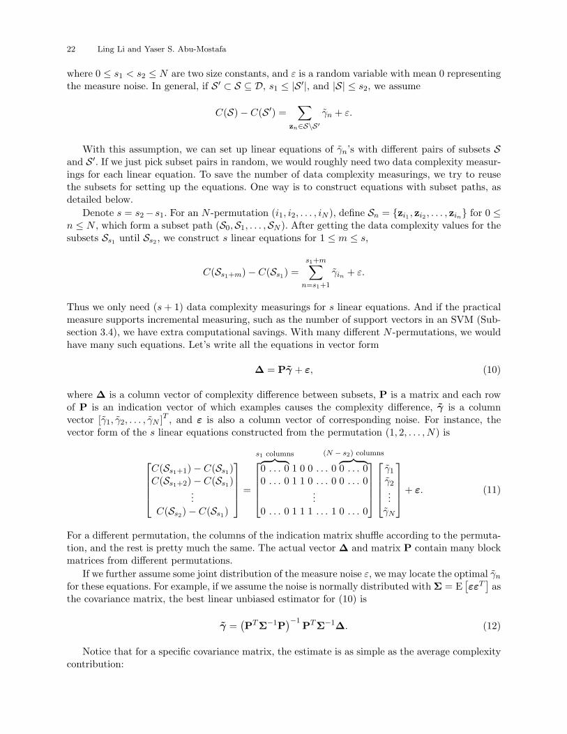
where ∆ is a column vector of complexity difference between subsets, P is a matrix and each rowof P is an indication vector of which examples causes the complexity difference, γ is a columnvector [γ1, γ2, . . . , γN ]T , and ε is also a column vector of corresponding noise. For instance, thevector form of the s linear equations constructed from the permutation (1, 2, . . . , N) is

C(Ss1+1)− C(Ss1)C(Ss1+2)− C(Ss1)

...C(Ss2)− C(Ss1)

=

s1 columns︷︸︸︷0 . . . 0 1 0 0 . . . 0

(N − s2) columns︷︸︸︷0 . . . 0

0 . . . 0 1 1 0 . . . 0 0 . . . 0...

0 . . . 0 1 1 1 . . . 1 0 . . . 0

γ1

γ2...

γN

+ ε. (11)

For a different permutation, the columns of the indication matrix shuffle according to the permuta-tion, and the rest is pretty much the same. The actual vector ∆ and matrix P contain many blockmatrices from different permutations.

If we further assume some joint distribution of the measure noise ε, we may locate the optimal γn

for these equations. For example, if we assume the noise is normally distributed with Σ = E[εεT

]as

the covariance matrix, the best linear unbiased estimator for (10) is

γ =(PTΣ−1P

)−1PTΣ−1∆. (12)

Notice that for a specific covariance matrix, the estimate is as simple as the average complexitycontribution:


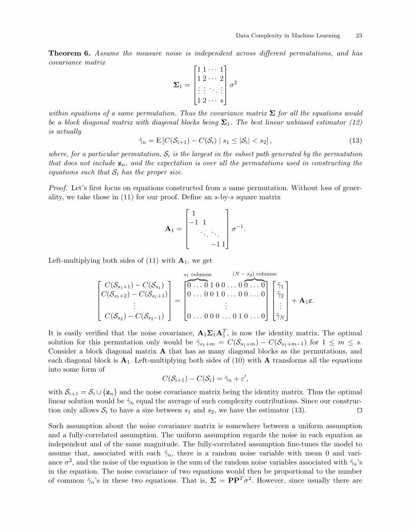
Theorem 6. Assume the measure noise is independent across different permutations, and hascovariance matrix

Σ1 =

1 1 · · · 11 2 · · · 2...

.... . .

...1 2 · · · s

σ2

within equations of a same permutation. Thus the covariance matrix Σ for all the equations wouldbe a block diagonal matrix with diagonal blocks being Σ1. The best linear unbiased estimator (12)is actually

γn = E [C(Si+1)− C(Si) | s1 ≤ |Si| < s2] , (13)

where, for a particular permutation, Si is the largest in the subset path generated by the permutationthat does not include zn, and the expectation is over all the permutations used in constructing theequations such that Si has the proper size.

Proof. Let’s first focus on equations constructed from a same permutation. Without loss of gener-ality, we take those in (11) for our proof. Define an s-by-s square matrix

A1 =

1−1 1

. . . . . .−1 1

σ−1.

Left-multiplying both sides of (11) with A1, we get

C(Ss1+1)− C(Ss1)

C(Ss1+2)− C(Ss1+1)...

C(Ss2)− C(Ss2−1)

=

s1 columns︷︸︸︷0 . . . 0 1 0 0 . . . 0

(N − s2) columns︷︸︸︷0 . . . 0

0 . . . 0 0 1 0 . . . 0 0 . . . 0...

0 . . . 0 0 0 . . . 0 1 0 . . . 0

γ1

γ2...

γN

+ A1ε.

It is easily verified that the noise covariance, A1Σ1AT1 , is now the identity matrix. The optimal

solution for this permutation only would be γs1+m = C(Ss1+m) − C(Ss1+m−1) for 1 ≤ m ≤ s.Consider a block diagonal matrix A that has as many diagonal blocks as the permutations, andeach diagonal block is A1. Left-multiplying both sides of (10) with A transforms all the equationsinto some form of

C(Si+1)− C(Si) = γn + ε′,

with Si+1 = Si ∪zn and the noise covariance matrix being the identity matrix. Thus the optimallinear solution would be γn equal the average of such complexity contributions. Since our construc-tion only allows Si to have a size between s1 and s2, we have the estimator (13). ut

Such assumption about the noise covariance matrix is somewhere between a uniform assumptionand a fully-correlated assumption. The uniform assumption regards the noise in each equation asindependent and of the same magnitude. The fully-correlated assumption fine-tunes the model toassume that, associated with each γn, there is a random noise variable with mean 0 and vari-ance σ2, and the noise of the equation is the sum of the random noise variables associated with γn’sin the equation. The noise covariance of two equations would then be proportional to the numberof common γn’s in these two equations. That is, Σ = PPT σ2. However, since usually there are


more equations than unknown variables, Σ is singular, which gives trouble in solving the equationsvia (12). Although the actual noise covariance would depend many factors including the practicalcomplexity measure, it happens that the assumption that leads to average complexity contribu-tion (13) works well in practice, as we will see in the next subsection.

5.3 Experiments

We test with the Yin-Yang target the concept of complexity contribution and the methods forestimating the complexity contribution. The experimental settings are similar to those used by Liet al. (2005). That is, a data set of size 400 is randomly generated, and the outputs of 40 examples(the last 10% indices) are further flipped as injected outliers.

We first verify that outliers would have higher complexity contributions on average than noiselessexamples. To do so, we pick a random subset path and compute the complexity increase along thepath. This is repeated many times and the complexity increase is averaged. Figure 11 shows suchaverage complexity contribution of noisy and noiseless examples versus the subset size. Here are

0 50 100 150 200 250 300 350 4000

0.5

1

1.5

2

2.5

3

Subset size

Com

plex

ity c

ontri

butio

n

noisynoiseless

Figure 11. Average complexity contribution of the noisy and the noiseless examples in the Yin-Yang data

some observations:

• Overall, the 40 noisy examples have apparently much higher average complexity contributionthan the 360 noiseless ones.

• When the subset size is really small (≤ 6), the noisy and the noiseless examples are indistin-guishable with respect to complexity contribution. There has to be more information about thetarget in order to tell which examples are noisy and which are not.

• The average contribution of the noiseless examples becomes smaller when the subset gets larger.This is because when the subset has more details about the target function, newly addednoiseless examples would have less chance to increase the data complexity.

• The average contribution of the noisy examples becomes larger when the subset gets larger,but it also seems converging to some value around 2.5. The reason of the contribution increaseis related to that of the contribution decrease of the noiseless examples. When there is more


correct information about the target function, an outlier would cause more complexity increasethan it would when there is less information.

• The two contribution curves have noticeable bends at the right ends. These are artifacts due tothe lack of distinct subsets when the subset size is close to the full size.

One way to use the complexity contribution for data pruning is to set a threshold θ and claim anyexample zn noisy if γn ≥ θ. For the uniform variance assumption and the assumption leading to theaverage complexity contribution, which were discussed in Subsection 5.2, we set s1 = 50, s2 = 400,and solve equations created from 200,000 random permutations. We plot their receiver operatingcharacteristic (ROC) in Figure 12. The ROC summarizes how the false negative rate (portion ofnoisy examples being claimed as noiseless) changes with the false positive rate (portion of noiselessexamples being claimed as noisy) as the threshold θ varies. Both methods achieve large area underthe ROC curve (AUC), a criterion to compare different ROC curves.

0 0.2 0.4 0.6 0.8 10

0.2

0.4

0.6

0.8

1

False positive rate

1 −

fals

e ne

gativ

e ra

te

uniform assumption (AUC: 0.97111)average contribution (AUC: 0.97278)

Figure 12. ROC curves of two estimators on the Yin-Yang data

Similar to the data categorization proposed by Li et al. (2005), we also group all the trainingexamples into three categories: typical, critical, and noisy. With two ad hoc thresholds θ1 = 2

3and θ2 = 1, the typical examples are those with γn < θ1, and we hope they are actually noiselessand far from the class boundary; the noisy examples are those with γn > θ2, and we hope they areactually outliers; the critical examples are those have γn between θ1 and θ2, and we hope they areclose to the class boundary. Figure 13 is the fingerprint plot which visually shows the categorization.The examples are positioned according to their signed distance to the decision boundary on thevertical axis and their index n in the training set on the horizontal axis. Critical and noisy examplesare shown as empty circles and filled squares, respectively. We can see that most of the outliers(last 10% of the examples) are categorized as noisy, and some examples around the zero distancevalue are categorized as critical. We also have some imperfections—some of the critical examplesare categorized as outliers and vice versa.


0 50 100 150 200 250 300 350 400−1

−0.8

−0.6

−0.4

−0.2

0

0.2

0.4

0.6

0.8

1

Example index

Intri

nsic

val

ue

Figure 13. Fingerprint plot of the Yin-Yang data with the average contribution: · typical; critical; noisy

5.4 Discussion

With the estimated complexity contribution γn, we hope that a noiseless example would havea relatively low contribution and an outlier would have a relatively high contribution. However,whether an outlier can be distinguished using the complexity contribution heavily depends on thechoice of the subsets used in the linear equations as well as many other factors.

For instance, the smaller Yin-Yang data set (Figure 7 on page 15) contains several examplesin the small gray disk. It is reflected in the selected principal subsets (Figure 9 on page 17, alsoFigure 16 on page 32) that those examples are included in principal subsets of only relatively highdata complexity (≥ 35). Since those examples constitute a small percentage of the training set, arandom subset of size smaller than, say, half of the full training set size, has a small probability tohave most of those examples, and would usually only have patterns shown in principal subsets withdata complexity lower than 35. Thus those examples would have large complexity contributionswith high probability. For similar reasons, if some outliers happen to be in the small gray disk ofthe Yin-Yang target, with small subsets they may be regarded as innocent.

It is still unclear what conditions can assure that an outlier would have a high average complexitycontribution.

5.5 Related Work

The complexity contribution quantifies to what degree an example may affect learning with respectto the data complexity. It is similar to the information gain concept behind informative examplesused by Guyon et al. (1996) for outlier detection.

Some other outlier detection methods also exploit practical data complexity measures. Gam-berger and Lavrac (1997) used a saturation test which is quite similar to our greedy method. Arninget al. (1996) looked for the greatest reduction in complexity by removing a subset of examples, whichcan be approximately explained by the proposition 2 in Theorem 5.

Statistics community has studied outlier detection extensively (Barnett and Lewis, 1994). Theyusually assume an underlying statistical model and define outliers based on discordance tests, manyof which can be described as some simple distance-based check (Knorr and Ng, 1997).


Learning algorithms can also be used for data pruning. For example, Angelova et al. (2005)combined many classifiers with naive Bayes learning for identifying troublesome examples. Somelearning algorithms, such as boosting, can produce information about the hardness of an exampleas a byproduct, which can be used for outlier detection (Merler et al., 2004; Li et al., 2005).

Angiulli et al. (2004) encoded background knowledge in the form of a first-order logic theory andoutliers were defined as examples for which no logical justification can be found in the theory. Theyalso showed that such outlier detection was intrinsically intractable due to its high computationalcomplexity.

6 Conclusion

We have defined three ideal complexity measures for a data set. The universal data complexityis the length of the shortest program that can replicate the data set. The data complexity for alearning model finds a consistent hypothesis with the shortest encoding. And the data complexitywith a lookup table also takes hypothesis errors into consideration. All these complexity measuresare closely related to learning principles such as Occam’s razor.

We have demonstrated the usage of the data complexity in two machine learning problems, datadecomposition and data pruning. In data decomposition, we have illustrated that the principal sub-sets best approximate the full data set; in data pruning, we have proved that outliers are exampleswith high complexity contributions. We have also proposed and tested methods for estimating thecomplexity contribution.

Underneath the concept and the applications of the data complexity is the desire for general-ization, the central issue of machine learning. Theoretically, if the correct prior and the exact noisemodel are known, we can encode the hypotheses and the errors in a way such that the shortesthypothesis generalizes the best. If the prior is unknown, the universal prior is a good guess for anycomputable priors, and the shortest hypothesis would still have high chance to generalize well. Inpractice, we also make a reasonable guess on the prior since practical approximations are usuallydesigned with Occam’s razor in mind.

Many approaches in this paper require intensive computational efforts, which is inevitable whenthe shortest hypothesis is sought. However, for practical applications, more computationally feasiblesolutions should be studied.

Acknowledgments

We wish to thank Xin Yu, Amrit Pratap, and Hsuan-Tien Lin for great suggestions and helpfulcomments. This work was partially supported by the Caltech SISL Graduate Fellowship.

References

Abu-Mostafa, Y. S. (1988a). Complexity of random problems. In Abu-Mostafa, Y. S., editor,Complexity in Information Theory, pages 115–131. Springer-Verlag.

Abu-Mostafa, Y. S. (1988b). Random problems. Journal of Complexity, 4(4):277–284.Abu-Mostafa, Y. S. (1995). Hints. Neural Computation, 7(4):639–671.Aizerman, M., Braverman, E., and Rozonoer, L. (1964). Theoretical foundations of the potential

function method in pattern recognition learning. Automation and Remote Control, 25(6):821–837.Angelova, A., Abu-Mostafa, Y., and Perona, P. (2005). Pruning training sets for learning of object

categories. In Schmid, C., Soatto, S., and Tomasi, C., editors, IEEE Computer Society Conferenceon Computer Vision and Pattern Recognition (CVPR 2005), volume 1, pages 494–501.


Angiulli, F., Greco, G., and Palopoli, L. (2004). Detecting outliers via logical theories and itsdata complexity. In Suzuki, E. and Arikawa, S., editors, Discovery Science: 7th InternationalConference, DS 2004, volume 3245 of Lecture Notes in Artificial Intelligence, pages 101–113.Springer-Verlag.

Arning, A., Agrawal, R., and Raghavan, P. (1996). A linear method for deviation detection inlarge databases. In Simoudis, E., Han, J., and Fayyad, U., editors, Proceedings of the SecondInternational Conference on Knowledge Discovery & Data Mining, pages 164–169. AAAI Press.

Barnett, V. and Lewis, T. (1994). Outliers in Statistical Data. John Wiley & Sons, 3rd edition.Bishop, C. M. (1995). Neural Networks for Pattern Recognition. Oxford University Press.Blumer, A., Ehrenfeucht, A., Haussler, D., and Warmuth, M. K. (1987). Occam’s razor. Information

Processing Letters, 24(6):377–380.Brodley, C. E. and Friedl, M. A. (1999). Identifying mislabeled training data. Journal of Artificial

Intelligence Research, 11:131–167.Cauwenberghs, G. and Poggio, T. (2001). Incremental and decremental support vector machine

learning. In Leen, T. K., Dietterich, T. G., and Tresp, V., editors, Advances in Neural InformationProcessing Systems 13, pages 409–415. MIT Press.

Gamberger, D. and Lavrac, N. (1997). Conditions for Occam’s razor applicability and noise elimi-nation. In van Someren, M. and Widmer, G., editors, Machine Learning: ECML-97, volume 1224of Lecture Notes in Artificial Intelligence, pages 108–123. Springer-Verlag.

Grunwald, P. (2005). Minimum description length tutorial. In Grunwald, P. D., Myung, I. J.,and Pitt, M. A., editors, Advances in Minimum Description Length: Theory and Applications,chapter 2, pages 23–80. MIT Press.

Guyon, I., Matic, N., and Vapnik, V. (1996). Discovering informative patterns and data cleaning.In Fayyad, U. M., Piatetsky-Shapiro, G., Smyth, P., and Uthurusamy, R., editors, Advances inKnowledge Discovery and Data Mining, pages 181–203. AAAI Press/MIT Press.

Hammer, P. L., Kogan, A., Simeone, B., and Szedmak, S. (2004). Pareto-optimal patterns in logicalanalysis of data. Discrete Applied Mathematics, 144(1–2):79–102.

Hodge, V. J. and Austin, J. (2004). A survey of outlier detection methodologies. Artificial Intelli-gence Review, 22(2):85–126.

Knorr, E. M. and Ng, R. T. (1997). A unified notion of outliers: Properties and computation.In Heckerman, D., Mannila, H., Pregibon, D., and Uthurusamy, R., editors, Proceedings of theThird International Conference on Knowledge Discovery and Data Mining, pages 219–222. AAAIPress.

Levin, L. A. (1973). Universal sequential search problems. Problems of Information Transmission,9(3):265–266.

Li, L., Pratap, A., Lin, H.-T., and Abu-Mostafa, Y. S. (2005). Improving generalization by datacategorization. In Jorge, A., Torgo, L., Brazdil, P., Camacho, R., and Gama, J., editors, Knowl-edge Discovery in Databases: PKDD 2005, volume 3721 of Lecture Notes in Artificial Intelligence,pages 157–168. Springer-Verlag.

Li, M. and Vitanyi, P. (1997). An Introduction to Kolmogorov Complexity and Its Applications.Springer-Verlag, 2nd edition.

Lin, H.-T. and Li, L. (2005a). Infinite ensemble learning with support vector machines. In Gama,J., Camacho, R., Brazdil, P., Jorge, A., and Torgo, L., editors, Machine Learning: ECML 2005,volume 3720 of Lecture Notes in Artificial Intelligence, pages 242–254. Springer-Verlag.

Lin, H.-T. and Li, L. (2005b). Novel distance-based SVM kernels for infinite ensemble learning.In Proceedings of the 12th International Conference on Neural Information Processing, pages761–766.

Merler, S., Caprile, B., and Furlanello, C. (2004). Bias-variance control via hard points shaving.International Journal of Pattern Recognition and Artificial Intelligence, 18(5):891–903.


Nicholson, A. (2002). Generalization Error Estimates and Training Data Valuation. PhD thesis,California Institute of Technology.

Quinlan, J. R. (1986). Induction of decision trees. Machine Learning, 1(1):81–106.Rissanen, J. (1978). Modeling by shortest data description. Automatica, 14(5):465–471.Schmidhuber, J. (1997). Discovering neural nets with low Kolmogorov complexity and high gener-

alization capability. Neural Networks, 10(5):857–873.Solomonoff, R. J. (2003). The universal distribution and machine learning. The Computer Journal,

46(6):598–601.Vapnik, V. N. (1999). The Nature of Statistical Learning Theory. Springer-Verlag, 2nd edition.Webb, G. I. (1996). Further experimental evidence against the utility of Occam’s razor. Journal

of Artificial Intelligence Research, 4:397–417.Wolpert, D. H. and Macready, W. G. (1999). Self-dissimilarity: An empirically observable com-

plexity measure. In Bar-Yam, Y., editor, Unifying Themes in Complex Systems, pages 626–643.Perseus Books.

Zupan, B., Bohanec, M., Bratko, I., and Demsar, J. (1997). Machine learning by function de-composition. In Douglas H. Fisher, J., editor, Machine Learning: Proceedings of the FourteenthInternational Conference (ICML ’97), pages 421–429. Morgan Kaufmann.

Zupan, B., Bratko, I., Bohanec, M., and Demsar, J. (2001). Function decomposition in machinelearning. In Paliouras, G., Karkaletsis, V., and Spyropoulos, C. D., editors, Machine Learningand Its Applications: Advanced Lectures, volume 2049 of Lecture Notes in Artificial Intelligence,pages 71–101. Springer-Verlag.

A Principal Sets

Here we collect all the principal subsets of the concentric disks problem (Figure 14) and almostall the principal subsets of the Yin-Yang problem (Figures 15 and 16), which are described inSubsection 4.3. The corresponding complexity-error plots can be found in Figure 5 on page 14and Figure 8 on page 16. For the Yin-Yang problem, each of the principal points (11, 16), (15, 12),and (16, 11) has 4 or more associated principal subsets, but only two are shown for space reason.The number of support vectors in SVM-perceptron is the practical data complexity measure used.


(0, 11) (7, 10) (8, 9) (8, 9)

(9, 7) (11, 6) (14, 5) (14, 5)

(14, 5) (14, 5) (15, 4) (17, 3)

(19, 2) (23, 1) (23, 1) (23, 1)

(24, 0)

Figure 14. All principal subsets of the concentric disks problem (complexity-error pairs are also listed)


(0, 47) (4, 43) (5, 34) (5, 34)

(6, 30) (6, 30) (7, 24) (8, 22)

(9, 20) (10, 17) (11, 16) (11, 16)

(12, 15) (12, 15) (12, 15) (13, 14)

(13, 14) (14, 13) (15, 12) (15, 12)

Figure 15. Principal subsets of the Yin-Yang data, part I


(16, 11) (16, 11) (17, 10) (19, 9)

(19, 9) (19, 9) (21, 8) (21, 8)

(23, 7) (23, 7) (23, 7) (24, 6)

(28, 5) (28, 5) (29, 4) (35, 3)

(35, 3) (36, 2) (40, 1) (41, 0)

Figure 16. Principal subsets of the Yin-Yang data, part II

data complexity in machine learning - …authors.library.caltech.edu/27081/1/dcomplex.pdfdata...

Documents