data, covariance, and correlation matrix -...
TRANSCRIPT
Data, Covariance, and Correlation Matrix
Nathaniel E. Helwig
Assistant Professor of Psychology and StatisticsUniversity of Minnesota (Twin Cities)
Updated 16-Jan-2017
Nathaniel E. Helwig (U of Minnesota) Data, Covariance, and Correlation Matrix Updated 16-Jan-2017 : Slide 1

Copyright
Copyright c© 2017 by Nathaniel E. Helwig
Nathaniel E. Helwig (U of Minnesota) Data, Covariance, and Correlation Matrix Updated 16-Jan-2017 : Slide 2

Outline of Notes
1) The Data MatrixDefinitionPropertiesR code
2) The Covariance MatrixDefinitionPropertiesR code
3) The Correlation MatrixDefinitionPropertiesR code
4) Miscellaneous TopicsCrossproduct calculationsVec and KroneckerVisualizing data
Nathaniel E. Helwig (U of Minnesota) Data, Covariance, and Correlation Matrix Updated 16-Jan-2017 : Slide 3

The Data Matrix
The Data Matrix
Nathaniel E. Helwig (U of Minnesota) Data, Covariance, and Correlation Matrix Updated 16-Jan-2017 : Slide 4
The Data Matrix Definition
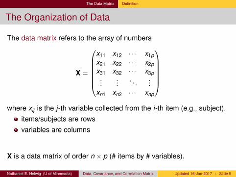
The Organization of Data
The data matrix refers to the array of numbers
X =
x11 x12 · · · x1px21 x22 · · · x2px31 x32 · · · x3p...
.... . .
...xn1 xn2 · · · xnp
where xij is the j-th variable collected from the i-th item (e.g., subject).
items/subjects are rowsvariables are columns
X is a data matrix of order n × p (# items by # variables).
Nathaniel E. Helwig (U of Minnesota) Data, Covariance, and Correlation Matrix Updated 16-Jan-2017 : Slide 5

The Data Matrix Definition
Collection of Column Vectors
We can view a data matrix as a collection of column vectors:
X =
x1 x2 · · · xp
where xj is the j-th column of X for j ∈ {1, . . . ,p}.
The n × 1 vector xj gives the j-th variable’s scores for the n items.
Nathaniel E. Helwig (U of Minnesota) Data, Covariance, and Correlation Matrix Updated 16-Jan-2017 : Slide 6
The Data Matrix Definition
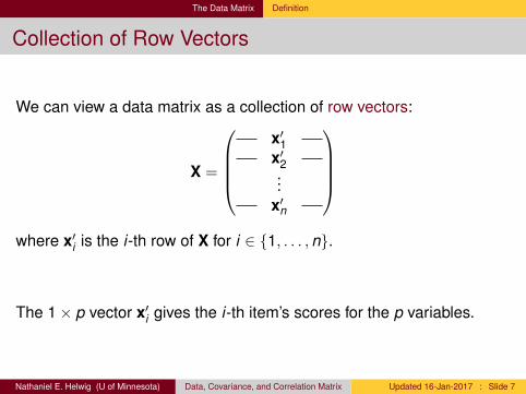
Collection of Row Vectors
We can view a data matrix as a collection of row vectors:
X =
x′1x′2...
x′n
where x′i is the i-th row of X for i ∈ {1, . . . ,n}.
The 1× p vector x′i gives the i-th item’s scores for the p variables.
Nathaniel E. Helwig (U of Minnesota) Data, Covariance, and Correlation Matrix Updated 16-Jan-2017 : Slide 7

The Data Matrix Properties
Calculating Variable (Column) Means
The sample mean of the j-th variable is given by
x̄j =1n
n∑i=1
xij
= n−11′nxj
where1n denotes an n × 1 vector of onesxj denotes the j-th column of X
Nathaniel E. Helwig (U of Minnesota) Data, Covariance, and Correlation Matrix Updated 16-Jan-2017 : Slide 8

The Data Matrix Properties
Calculating Item (Row) Means
The sample mean of the i-th item is given by
x̄i =1p
p∑j=1
xij
= p−1x′i1p
where1p denotes an p × 1 vector of onesx′i denotes the i-th row of X
Nathaniel E. Helwig (U of Minnesota) Data, Covariance, and Correlation Matrix Updated 16-Jan-2017 : Slide 9

The Data Matrix R Code
Data Frame and Matrix Classes in R
> data(mtcars)> class(mtcars)[1] "data.frame"> dim(mtcars)[1] 32 11> head(mtcars)
mpg cyl disp hp drat wt qsec vs am gear carbMazda RX4 21.0 6 160 110 3.90 2.620 16.46 0 1 4 4Mazda RX4 Wag 21.0 6 160 110 3.90 2.875 17.02 0 1 4 4Datsun 710 22.8 4 108 93 3.85 2.320 18.61 1 1 4 1Hornet 4 Drive 21.4 6 258 110 3.08 3.215 19.44 1 0 3 1Hornet Sportabout 18.7 8 360 175 3.15 3.440 17.02 0 0 3 2Valiant 18.1 6 225 105 2.76 3.460 20.22 1 0 3 1> X <- as.matrix(mtcars)> class(X)[1] "matrix"
Nathaniel E. Helwig (U of Minnesota) Data, Covariance, and Correlation Matrix Updated 16-Jan-2017 : Slide 10

The Data Matrix R Code
Row and Column Means
> # get row means (3 ways)> rowMeans(X)[1:3]
Mazda RX4 Mazda RX4 Wag Datsun 71029.90727 29.98136 23.59818
> c(mean(X[1,]), mean(X[2,]), mean(X[3,]))[1] 29.90727 29.98136 23.59818> apply(X,1,mean)[1:3]
Mazda RX4 Mazda RX4 Wag Datsun 71029.90727 29.98136 23.59818
> # get column means (3 ways)> colMeans(X)[1:3]
mpg cyl disp20.09062 6.18750 230.72188> c(mean(X[,1]), mean(X[,2]), mean(X[,3]))[1] 20.09062 6.18750 230.72188> apply(X,2,mean)[1:3]
mpg cyl disp20.09062 6.18750 230.72188
Nathaniel E. Helwig (U of Minnesota) Data, Covariance, and Correlation Matrix Updated 16-Jan-2017 : Slide 11

The Data Matrix R Code
Other Row and Column Functions
> # get column medians> apply(X,2,median)[1:3]mpg cyl disp19.2 6.0 196.3> c(median(X[,1]), median(X[,2]), median(X[,3]))[1] 19.2 6.0 196.3
> # get column ranges> apply(X,2,range)[,1:3]
mpg cyl disp[1,] 10.4 4 71.1[2,] 33.9 8 472.0> cbind(range(X[,1]), range(X[,2]), range(X[,3]))
[,1] [,2] [,3][1,] 10.4 4 71.1[2,] 33.9 8 472.0
Nathaniel E. Helwig (U of Minnesota) Data, Covariance, and Correlation Matrix Updated 16-Jan-2017 : Slide 12
The Covariance Matrix
The Covariance Matrix
Nathaniel E. Helwig (U of Minnesota) Data, Covariance, and Correlation Matrix Updated 16-Jan-2017 : Slide 13

The Covariance Matrix Definition
The Covariation of Data
The covariance matrix refers to the symmetric array of numbers
S =
s2
1 s12 s13 · · · s1ps21 s2
2 s23 · · · s2ps31 s32 s2
3 · · · s3p...
......
. . ....
sp1 sp2 sp3 · · · s2p
where
s2j = (1/n)
∑ni=1(xij − x̄j)
2 is the variance of the j-th variable
sjk = (1/n)∑n
i=1(xij − x̄j)(xik − x̄k ) is the covariance between thej-th and k -th variablesx̄j = (1/n)
∑ni=1 xij is the mean of the j-th variable
Nathaniel E. Helwig (U of Minnesota) Data, Covariance, and Correlation Matrix Updated 16-Jan-2017 : Slide 14

The Covariance Matrix Definition
Covariance Matrix from Data Matrix
We can calculate the covariance matrix such as
S =1n
X′cXc
where Xc = X− 1nx̄′ = CX withx̄′ = (x̄1, . . . , x̄p) denoting the vector of variable meansC = In − n−11n1′n denoting a centering matrix
Note that the centered matrix Xc has the form
Xc =
x11 − x̄1 x12 − x̄2 · · · x1p − x̄px21 − x̄1 x22 − x̄2 · · · x2p − x̄px31 − x̄1 x32 − x̄2 · · · x3p − x̄p
......
. . ....
xn1 − x̄1 xn2 − x̄2 · · · xnp − x̄p
Nathaniel E. Helwig (U of Minnesota) Data, Covariance, and Correlation Matrix Updated 16-Jan-2017 : Slide 15

The Covariance Matrix Properties
Variances are Nonnegative
Variances are sums-of-squares, which implies that s2j ≥ 0 ∀j .
s2j > 0 as long as there does not exist an α such that xj = α1n
This implies that. . .tr(S) ≥ 0 where tr(·) denotes the matrix trace function∑p
j=1 λj ≥ 0 where (λ1, . . . , λp) are the eigenvalues of S
If n < p, then λj = 0 for at least one j ∈ {1, . . . ,p}. If n ≥ p and the pcolumns of X are linearly independent, then λj > 0 for all j ∈ {1, . . . ,p}.
Nathaniel E. Helwig (U of Minnesota) Data, Covariance, and Correlation Matrix Updated 16-Jan-2017 : Slide 16

The Covariance Matrix Properties
The Cauchy-Schwarz Inequality
From the Cauchy-Schwarz inequality we have that
s2jk ≤ s2
j s2k
with the equality holding if and only if xj and xk are linearly dependent.
We could also write the Cauchy-Schwarz inequality as
|sjk | ≤ sjsk
where sj and sk denote the standard deviations of the variables.
Nathaniel E. Helwig (U of Minnesota) Data, Covariance, and Correlation Matrix Updated 16-Jan-2017 : Slide 17

The Covariance Matrix R Code
Covariance Matrix by Hand (hard way)
> n <- nrow(X)> C <- diag(n) - matrix(1/n, n, n)> Xc <- C %*% X> S <- t(Xc) %*% Xc / (n-1)> S[1:3,1:6]
mpg cyl disp hp drat wtmpg 36.324103 -9.172379 -633.0972 -320.7321 2.1950635 -5.116685cyl -9.172379 3.189516 199.6603 101.9315 -0.6683669 1.367371disp -633.097208 199.660282 15360.7998 6721.1587 -47.0640192 107.684204
# or #
> Xc <- scale(X, center=TRUE, scale=FALSE)> S <- t(Xc) %*% Xc / (n-1)> S[1:3,1:6]
mpg cyl disp hp drat wtmpg 36.324103 -9.172379 -633.0972 -320.7321 2.1950635 -5.116685cyl -9.172379 3.189516 199.6603 101.9315 -0.6683669 1.367371disp -633.097208 199.660282 15360.7998 6721.1587 -47.0640192 107.684204
Nathaniel E. Helwig (U of Minnesota) Data, Covariance, and Correlation Matrix Updated 16-Jan-2017 : Slide 18

The Covariance Matrix R Code
Covariance Matrix using cov Function (easy way)
# calculate covariance matrix> S <- cov(X)> dim(S)[1] 11 11
# check variance> S[1,1][1] 36.3241> var(X[,1])[1] 36.3241> sum((X[,1]-mean(X[,1]))^2) / (n-1)[1] 36.3241
# check covariance> S[1:3,1:6]
mpg cyl disp hp drat wtmpg 36.324103 -9.172379 -633.0972 -320.7321 2.1950635 -5.116685cyl -9.172379 3.189516 199.6603 101.9315 -0.6683669 1.367371disp -633.097208 199.660282 15360.7998 6721.1587 -47.0640192 107.684204
Nathaniel E. Helwig (U of Minnesota) Data, Covariance, and Correlation Matrix Updated 16-Jan-2017 : Slide 19

The Correlation Matrix
The Correlation Matrix
Nathaniel E. Helwig (U of Minnesota) Data, Covariance, and Correlation Matrix Updated 16-Jan-2017 : Slide 20

The Correlation Matrix Definition
The Correlation of Data
The correlation matrix refers to the symmetric array of numbers
R =
1 r12 r13 · · · r1p
r21 1 r23 · · · r2pr31 r32 1 · · · r3p...
......
. . ....
rp1 rp2 rp3 · · · 1
where
rjk =sjk
sjsk=
∑ni=1(xij − x̄j)(xik − x̄k )√∑n
i=1(xij − x̄j)2√∑n
i=1(xik − x̄k )2
is the Pearson correlation coefficient between variables xj and xk .
Nathaniel E. Helwig (U of Minnesota) Data, Covariance, and Correlation Matrix Updated 16-Jan-2017 : Slide 21

The Correlation Matrix Definition
Correlation Matrix from Data Matrix
We can calculate the correlation matrix such as
R =1n
X′sXs
where Xs = CXD−1 withC = In − n−11n1′n denoting a centering matrixD = diag(s1, . . . , sp) denoting a diagonal scaling matrix
Note that the standardized matrix Xs has the form
Xs =
(x11 − x̄1)/s1 (x12 − x̄2)/s2 · · · (x1p − x̄p)/sp(x21 − x̄1)/s1 (x22 − x̄2)/s2 · · · (x2p − x̄p)/sp(x31 − x̄1)/s1 (x32 − x̄2)/s2 · · · (x3p − x̄p)/sp
......
. . ....
(xn1 − x̄1)/s1 (xn2 − x̄2)/s2 · · · (xnp − x̄p)/sp
Nathaniel E. Helwig (U of Minnesota) Data, Covariance, and Correlation Matrix Updated 16-Jan-2017 : Slide 22
The Correlation Matrix Properties
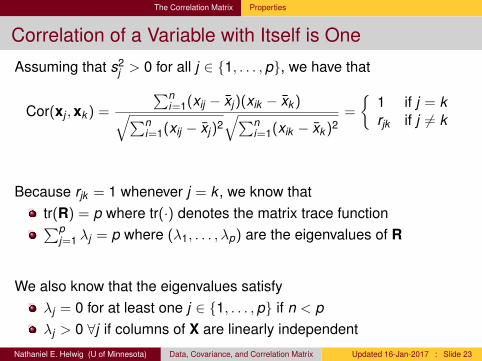
Correlation of a Variable with Itself is One
Assuming that s2j > 0 for all j ∈ {1, . . . ,p}, we have that
Cor(xj ,xk ) =
∑ni=1(xij − x̄j)(xik − x̄k )√∑n
i=1(xij − x̄j)2√∑n
i=1(xik − x̄k )2=
{1 if j = krjk if j 6= k
Because rjk = 1 whenever j = k , we know thattr(R) = p where tr(·) denotes the matrix trace function∑p
j=1 λj = p where (λ1, . . . , λp) are the eigenvalues of R
We also know that the eigenvalues satisfyλj = 0 for at least one j ∈ {1, . . . ,p} if n < pλj > 0 ∀j if columns of X are linearly independent
Nathaniel E. Helwig (U of Minnesota) Data, Covariance, and Correlation Matrix Updated 16-Jan-2017 : Slide 23

The Correlation Matrix Properties
The Cauchy-Schwarz Inequality (revisited)
Reminder: the Cauchy-Schwarz inequality implies that
s2jk ≤ s2
j s2k
with the equality holding if and only if xj and xk are linearly dependent.
Rearranging the terms, we have that
s2jk
s2j s2
k≤ 1 ←→ r2
jk ≤ 1
which implies that |rjk | ≤ 1 with equality holding if and only ifxj = α1n + βxk for some scalars α ∈ R and β ∈ R.
Nathaniel E. Helwig (U of Minnesota) Data, Covariance, and Correlation Matrix Updated 16-Jan-2017 : Slide 24
The Correlation Matrix R Code
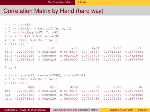
Correlation Matrix by Hand (hard way)
> n <- nrow(X)> C <- diag(n) - matrix(1/n, n, n)> D <- diag(apply(X, 2, sd))> Xs <- C %*% X %*% solve(D)> R <- t(Xs) %*% Xs / (n-1)> R[1:3,1:6]
[,1] [,2] [,3] [,4] [,5] [,6][1,] 1.0000000 -0.8521620 -0.8475514 -0.7761684 0.6811719 -0.8676594[2,] -0.8521620 1.0000000 0.9020329 0.8324475 -0.6999381 0.7824958[3,] -0.8475514 0.9020329 1.0000000 0.7909486 -0.7102139 0.8879799
# or #
> Xs <- scale(X, center=TRUE, scale=TRUE)> R <- t(Xs) %*% Xs / (n-1)> R[1:3,1:6]
mpg cyl disp hp drat wtmpg 1.0000000 -0.8521620 -0.8475514 -0.7761684 0.6811719 -0.8676594cyl -0.8521620 1.0000000 0.9020329 0.8324475 -0.6999381 0.7824958disp -0.8475514 0.9020329 1.0000000 0.7909486 -0.7102139 0.8879799
Nathaniel E. Helwig (U of Minnesota) Data, Covariance, and Correlation Matrix Updated 16-Jan-2017 : Slide 25

The Correlation Matrix R Code
Correlation Matrix using cor Function (easy way)
# calculate correlation matrix> R <- cor(X)> dim(R)[1] 11 11
# check correlation of mpg and cyl> R[1,2][1] -0.852162> cor(X[,1],X[,2])[1] -0.852162> cov(X[,1],X[,2]) / (sd(X[,1]) * sd(X[,2]))[1] -0.852162
# check correlations> R[1:3,1:6]
mpg cyl disp hp drat wtmpg 1.0000000 -0.8521620 -0.8475514 -0.7761684 0.6811719 -0.8676594cyl -0.8521620 1.0000000 0.9020329 0.8324475 -0.6999381 0.7824958disp -0.8475514 0.9020329 1.0000000 0.7909486 -0.7102139 0.8879799
Nathaniel E. Helwig (U of Minnesota) Data, Covariance, and Correlation Matrix Updated 16-Jan-2017 : Slide 26

Miscellaneous Topics
Miscellaneous Topics
Nathaniel E. Helwig (U of Minnesota) Data, Covariance, and Correlation Matrix Updated 16-Jan-2017 : Slide 27

Miscellaneous Topics Crossproduct Calculations
Two Types of Matrix Crossproducts
We often need to calculate one of two different types of crossproducts:X′Y = “regular” crossproduct of X and YXY′ = “transpose” crossproduct of X and Y
Regular crossproduct is X′ being post-multipled by Y.
Transpose crossproduct is X being post-multipled by Y′.
Nathaniel E. Helwig (U of Minnesota) Data, Covariance, and Correlation Matrix Updated 16-Jan-2017 : Slide 28

Miscellaneous Topics Crossproduct Calculations
Simple and Efficient Crossproducts in R
> X <- matrix(rnorm(2*3),2,3)> Y <- matrix(rnorm(2*3),2,3)> t(X) %*% Y
[,1] [,2] [,3][1,] 0.1342302 -1.8181837 -1.107821[2,] 1.1014703 -0.6619466 -1.356606[3,] 0.8760823 -1.0077151 -1.340044> crossprod(X, Y)
[,1] [,2] [,3][1,] 0.1342302 -1.8181837 -1.107821[2,] 1.1014703 -0.6619466 -1.356606[3,] 0.8760823 -1.0077151 -1.340044> X %*% t(Y)
[,1] [,2][1,] 0.8364239 3.227566[2,] -1.3899946 -2.704184> tcrossprod(X, Y)
[,1] [,2][1,] 0.8364239 3.227566[2,] -1.3899946 -2.704184
Nathaniel E. Helwig (U of Minnesota) Data, Covariance, and Correlation Matrix Updated 16-Jan-2017 : Slide 29

Miscellaneous Topics Vec Operator and Kronecker Product
Turning a Matrix into a Vector
The vectorization (vec) operator turns a matrix into a vector:
vec(X) =(x11, x21, . . . , xn1, x12, . . . , xn2, . . . , x1p, . . . , xnp
)′where the vectorization is done column-by-column.
In R, we just use the combine function c to vectorize a matrix> X <- matrix(1:6,2,3)> X
[,1] [,2] [,3][1,] 1 3 5[2,] 2 4 6> c(X)[1] 1 2 3 4 5 6> c(t(X))[1] 1 3 5 2 4 6
Nathaniel E. Helwig (U of Minnesota) Data, Covariance, and Correlation Matrix Updated 16-Jan-2017 : Slide 30

Miscellaneous Topics Vec Operator and Kronecker Product
vec Operator Properties
Some useful properties of the vec(·) operator include:vec(a′) = vec(a) = a for any vector a ∈ Rm
vec(ab′) = b⊗ a for any vectors a ∈ Rm and b ∈ Rn
vec(A)′vec(B) = tr(A′B) for any matrices A,B ∈ Rm×n
vec(ABC) = (C′ ⊗ A)vec(B) if the product ABC exists
Note: ⊗ is the Kronecker product, which is defined on the next slide.
Nathaniel E. Helwig (U of Minnesota) Data, Covariance, and Correlation Matrix Updated 16-Jan-2017 : Slide 31

Miscellaneous Topics Vec Operator and Kronecker Product
Kronecker Product of Two Matrices
Given X = {xij}n×p and Y = {yij}m×q, the Kronecker product is
X⊗ Y =
x11Y x12Y · · · x1pYx21Y x22Y · · · x2pY
......
. . ....
xn1Y xn2Y · · · xnpY
which is a matrix of order mn × pq.
In R, the kronecker function calculates Kronecker products> X <- matrix(1:4,2,2)> Y <- matrix(5:10,2,3)> kronecker(X, Y)
[,1] [,2] [,3] [,4] [,5] [,6][1,] 5 7 9 15 21 27[2,] 6 8 10 18 24 30[3,] 10 14 18 20 28 36[4,] 12 16 20 24 32 40
Nathaniel E. Helwig (U of Minnesota) Data, Covariance, and Correlation Matrix Updated 16-Jan-2017 : Slide 32

Miscellaneous Topics Vec Operator and Kronecker Product
Kronecker Product Properties
Some useful properties of the Kronecker product include:1 A⊗ a = Aa = aA = a⊗ A for any a ∈ R and A ∈ Rm×n
2 (A⊗ B)′ = A′ ⊗ B′ for any matrices A ∈ Rm×n and B ∈ Rp×q
3 a′ ⊗ b = ba′ = b⊗ a′ for any vectors a ∈ Rm and b ∈ Rn
4 tr(A⊗ B) = tr(A)tr(B) for any matrices A ∈ Rm×m and B ∈ Rp×p
5 (A⊗ B)−1 = A−1 ⊗ B−1 for any invertible matrices A and B6 (A⊗ B)† = A† ⊗ B† where (·)† is Moore-Penrose pseudoinverse7 |A⊗ B| = |A|p|B|m for any matrices A ∈ Rm×m and B ∈ Rp×p
8 rank(A⊗ B) = rank(A)rank(B) for any matrices A and B9 A⊗ (B + C) = A⊗ B + A⊗ C for any matrices A, B, and C
10 (A + B)⊗ C = A⊗ C + B⊗ C for any matrices A, B, and C11 (A⊗ B)⊗ C = A⊗ (B⊗ C) for any matrices A, B, and C12 (A⊗ B)(C⊗ D) = (AC)⊗ (BD) for any matrices A, B, C, and D
Nathaniel E. Helwig (U of Minnesota) Data, Covariance, and Correlation Matrix Updated 16-Jan-2017 : Slide 33

Miscellaneous Topics Vec Operator and Kronecker Product
Common Application of Vec and Kronecker
Suppose the rows of X are iid samples from some multivariatedistribution with mean µ = (µ1, . . . , µp)′ and covariance matrix Σ.
xiiid∼ (µ,Σ) where xi is the i-th row of X
If we let y = vec(X′), then the expectation and covariance areE(y) = 1n ⊗ µ is the mean vectorV (y) = In ⊗Σ is the covariance matrix
Note that the covariance matrix is block diagonal
In ⊗Σ =
Σ 0 · · · 00 Σ · · · 0...
.... . .
...0 0 · · · Σ
given that data from different subjects are assumed to be independent.Nathaniel E. Helwig (U of Minnesota) Data, Covariance, and Correlation Matrix Updated 16-Jan-2017 : Slide 34

Miscellaneous Topics Visualizing Multivariate Data
Two Versions of a Scatterplot in R
●●
●
●
●●
●
●
●
●
●
●
●
●
● ●
●
●
●
●
●
●●
●
●
●
●
●
●
●
●
●
50 100 150 200 250 300
1015
2025
30
HP
MP
G
●
50 100 150 200 250 300
1015
2025
30
HPM
PG
●●
●
●
●
●
●
●
●
●
●
●
●
●
● ●
●
●
●
●
●
●●
●
●
●
●
●
●
●
●
●
plot(mtcars$hp, mtcars$mpg, xlab="HP", ylab="MPG")library(car)scatterplot(mtcars$hp, mtcars$mpg, xlab="HP", ylab="MPG")
Nathaniel E. Helwig (U of Minnesota) Data, Covariance, and Correlation Matrix Updated 16-Jan-2017 : Slide 35

Miscellaneous Topics Visualizing Multivariate Data
Two Versions of a Scatterplot Matrix in R
mpg
100 300
●●●
●
●
●
●
●●
●
●●
●●
●
●
●
●
●●
●
●
2 3 4 5
1015
2025
30
●●●
●
●
●
●
●●
●
●
100
300
●
●●
●● ●
●
●
●●
●
disp
●
● ●
●●●
●
●
●●●
●
●●
●●●
●
●
●●
●
●
●
●
●●
●
●
●
●●●
●
●
●
●●●
●
●
●● ●
hp
5015
025
0
●
●
●
●●
●
●
●
●● ●
10 15 20 25 30
23
45
●
●●
●
●●
●
●●
●
●
●
●●
●
●●
●
●●
●
●
50 150 250
●
● ●
●
●●
●
●●
●
●
wt
● 468
mpg
100 300
●●●
●
●
●
●
●●
●
●●
●●
●
●
●
●
●●
●
●
2 3 4 5
1015
2025
30
●●●
●
●
●
●
●●
●
●
100
300
●
●●
●● ●
●
●
●●
●
disp
●
● ●
●●●
●
●
●●●
●
●●
●●●
●
●
●●
●
●
●
●
●●
●
●
●
●●●
●
●
●
●●●
●
●
●● ●
hp
5015
025
0
●
●
●
●●
●
●
●
●● ●
10 15 20 25 302
34
5
●
●●
●
●●
●
●●
●
●
●
●●
●
●●
●
●●
●
●
50 150 250
●
● ●
●
●●
●
●●
●
●
wt
cylint <- as.integer(factor(mtcars$cyl))pairs(~mpg+disp+hp+wt, data=mtcars, col=cylint, pch=cylint)library(car)scatterplotMatrix(~mpg+disp+hp+wt|cyl, data=mtcars)
Nathaniel E. Helwig (U of Minnesota) Data, Covariance, and Correlation Matrix Updated 16-Jan-2017 : Slide 36

Miscellaneous Topics Visualizing Multivariate Data
Three-Dimensional Scatterplot in R
50 100 150 200 250 300 350
1015
2025
3035
1
2
3
4
5
6
HP
WTMP
G
●
●
●●
●
●
●●
●
● ●
50 100 150 200 250 300 350
1015
2025
3035
1
2
3
4
5
6
HP
WTMP
G
●
●
●●
●
●
●●
●
● ●
library(scatterplot3d)sp3d <- scatterplot3d(mtcars$hp, mtcars$wt, mtcars$mpg,
type="h", color=cylint, pch=cylint,xlab="HP", ylab="WT", zlab="MPG")
fitmod <- lm(mpg ~ hp + wt, data=mtcars)sp3d$plane3d(fitmod)
Nathaniel E. Helwig (U of Minnesota) Data, Covariance, and Correlation Matrix Updated 16-Jan-2017 : Slide 37

Miscellaneous Topics Visualizing Multivariate Data
Color Image (Heat Map) Plots in R
50 100 150 200 250 300
23
45
HP
WT
1015
2025
MP
G
50 100 150 200 250 300
23
45
HP
WT
fitmod <- lm(mpg ~ hp + wt, data=mtcars)hpseq <- seq(50, 330, by=20)wtseq <- seq(1.5, 5.4, length=15)newdata <- expand.grid(hp=hpseq, wt=wtseq)fit <- predict(fitmod, newdata)fitmat <- matrix(fit, 15, 15)image(hpseq, wtseq, fitmat, xlab="HP", ylab="WT")library(bigsplines)imagebar(hpseq, wtseq, fitmat, xlab="HP", ylab="WT", zlab="MPG", col=heat.colors(12), ncolor=12)
Nathaniel E. Helwig (U of Minnesota) Data, Covariance, and Correlation Matrix Updated 16-Jan-2017 : Slide 38

Miscellaneous Topics Visualizing Multivariate Data
Correlation Matrix Plot in R
●
● ●
●
●
●
●
●
●
●
●
●
●
●
●
●
●
●
●
●
●
●
●
●
●
●
●
●●
●
●
●
●
●
●
●
●
●
−1
−0.8
−0.6
−0.4
−0.2
0
0.2
0.4
0.6
0.8
1
mpg
cyl
disp
hp drat
wt
qsec
vs am gear
carb
mpg
cyl
disp
hp
drat
wt
qsec
vs
am
gear
carb−1
−0.8
−0.6
−0.4
−0.2
0
0.2
0.4
0.6
0.8
1
mpg
cyl
disp
hp
drat
wt
qsec
vs
am
gear
carb
−0.85
−0.85
−0.78
0.68
−0.87
0.42
0.66
0.6
0.48
−0.55
0.9
0.83
−0.7
0.78
−0.59
−0.81
−0.52
−0.49
0.53
0.79
−0.71
0.89
−0.43
−0.71
−0.59
−0.56
0.39
−0.45
0.66
−0.71
−0.72
−0.24
−0.13
0.75
−0.71
0.09
0.44
0.71
0.7
−0.09
−0.17
−0.55
−0.69
−0.58
0.43
0.74
−0.23
−0.21
−0.66
0.17
0.21
−0.57
0.79
0.06 0.27
cmat <- cor(mtcars)library(corrplot)corrplot(cmat, method="circle")corrplot.mixed(cmat, lower="number", upper="ellipse")
Nathaniel E. Helwig (U of Minnesota) Data, Covariance, and Correlation Matrix Updated 16-Jan-2017 : Slide 39
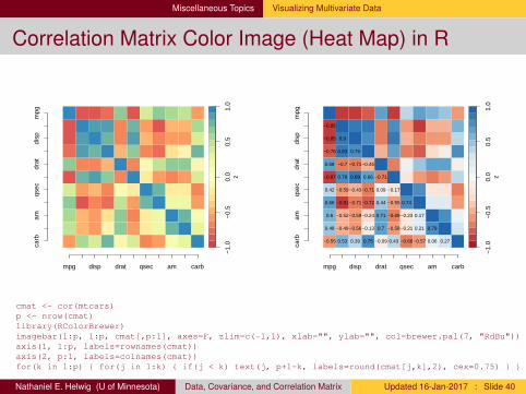
Miscellaneous Topics Visualizing Multivariate Data
Correlation Matrix Color Image (Heat Map) in R
−1.
0−
0.5
0.0
0.5
1.0
z
mpg disp drat qsec am carb
carb
amqs
ecdr
atdi
spm
pg
−1.
0−
0.5
0.0
0.5
1.0
z
mpg disp drat qsec am carb
carb
amqs
ecdr
atdi
spm
pg
−0.85
−0.85 0.9
−0.78 0.83 0.79
0.68 −0.7 −0.71−0.45
−0.87 0.78 0.89 0.66 −0.71
0.42 −0.59−0.43−0.71 0.09 −0.17
0.66 −0.81−0.71−0.72 0.44 −0.55 0.74
0.6 −0.52−0.59−0.24 0.71 −0.69−0.23 0.17
0.48 −0.49−0.56−0.13 0.7 −0.58−0.21 0.21 0.79
−0.55 0.53 0.39 0.75 −0.09 0.43 −0.66−0.57 0.06 0.27
cmat <- cor(mtcars)p <- nrow(cmat)library(RColorBrewer)imagebar(1:p, 1:p, cmat[,p:1], axes=F, zlim=c(-1,1), xlab="", ylab="", col=brewer.pal(7, "RdBu"))axis(1, 1:p, labels=rownames(cmat))axis(2, p:1, labels=colnames(cmat))for(k in 1:p) { for(j in 1:k) { if(j < k) text(j, p+1-k, labels=round(cmat[j,k],2), cex=0.75) } }
Nathaniel E. Helwig (U of Minnesota) Data, Covariance, and Correlation Matrix Updated 16-Jan-2017 : Slide 40