data diagnostics for introduction - ndsu · data diagnostics for introduction ... source df sum of...

DATA DIAGNOSTICS FOR Introduction

• One of the assumptions of ANOVA and Regression is that the errors should be independently and normally distributed.

• Randomization often is used to break up any correlation of experimental units.

• A problem that may influence this assumption is that the errors may be

heterogeneous.

• There are two types of heterogeneity.

1. Irregular: certain independent variables possess considerably more variability that others. e.g. In insecticide trials, the checks may contain considerably more insects that the treated experimental units; therefore, the checks contribute to the Error MS to a larger degree than the treated units. Consequently, the standard deviation will be too large for comparisons among treated experimental units.

a. This portion of the experiment is not under statistical control.

b. The best procedure to compensate for this problem is to omit certain portions of the data from the analysis or use orthogonal contrasts.

2. Regular: arises from some type of non-normality of the data in the experiment.

a. This non-normality is caused by a relationship between the variability of

several treatments and the mean.

b. To correct the problem, the data can be transformed such that the transformed errors are normally distributed.

Influential Data

• In addition to data that may violate the assumptions of the analysis you will be using, data can be problematic if they have undue impact on your results. There are three categories of problematic data:

1. Outliers: In terms of regression, an outlier is defined as an observation with a

large residual 𝑒! = 𝑌 − 𝑌!. a. Outliers can be caused by data entry mistakes or just unique or odd

observations.

2. Leverage: A measure of how far an observation deviates from the mean (𝑌! − 𝑌). These values can affect estimates of the regression coefficients.

3. Influence: An observation is deemed to have undue influence if the analysis conducted with the observation removed changes the estimates of the regression coefficients substantially.

a. Often influence is caused by outliers or a product of leverage.

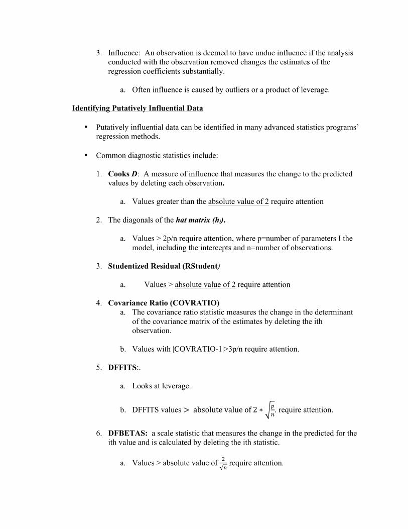
Identifying Putatively Influential Data

• Putatively influential data can be identified in many advanced statistics programs’ regression methods.

• Common diagnostic statistics include: 1. Cooks D: A measure of influence that measures the change to the predicted

values by deleting each observation.

a. Values greater than the absolute value of 2 require attention

2. The diagonals of the hat matrix (hi). a. Values > 2p/n require attention, where p=number of parameters I the

model, including the intercepts and n=number of observations.

3. Studentized Residual (RStudent)

a. Values > absolute value of 2 require attention

4. Covariance Ratio (COVRATIO) a. The covariance ratio statistic measures the change in the determinant

of the covariance matrix of the estimates by deleting the ith observation.

b. Values with |COVRATIO-1|>3p/n require attention.

5. DFFITS:.

a. Looks at leverage.

b. DFFITS values > absolute value of 2 ∗ !!. require attention.

6. DFBETAS: a scale statistic that measures the change in the predicted for the

ith value and is calculated by deleting the ith statistic.

a. Values > absolute value of !! require attention.

Example of Using Diagnostics for Simple Linear Regression

• SAS Commands

options pageno=1; input PLOT BLOC ENTRY HDDT HT LODG YIELD MOIST; datalines; 3501 1 8 32 84.5 3 46.8 21.5 3502 1 30 32 82.5 3 78.9 19.8 3503 1 7 31 73.5 3 68.5 20.7 3504 1 26 36 64.5 1 64.5 16.7 3505 1 13 33 75.5 2 69.8 16.4 3506 1 18 31 76.0 2 74.5 16.7 3507 1 27 31 78.0 2 85.5 18.0 3508 1 4 34 81.5 4 67.3 16.4 3509 1 29 30 72.0 2 77.4 16.2 3510 1 19 30 80.5 2 55.5 15.3 3511 1 23 34 70.0 4 68.4 15.0 3512 1 5 33 85.0 5 64.2 13.8 3513 1 2 32 87.0 4 71.2 14.7 3514 1 22 35 79.0 4 62.0 13.3 3515 1 25 36 89.5 4 66.0 14.8 3516 1 6 31 83.0 2 77.3 13.6 3517 1 17 33 83.5 3 99.4 16.6 3518 1 3 32 84.0 3 79.9 16.2 3519 1 24 33 82.5 1 83.1 18.0 3520 1 21 32 80.5 1 84.1 19.4 3521 1 20 31 80.5 2 81.5 19.6 3522 1 16 31 75.5 1 65.1 16.0 3523 1 1 32 88.0 3 67.3 19.4 3524 1 14 33 82.0 2 72.9 18.5 3525 1 28 31 79.5 1 89.9 20.6 3526 1 10 31 85.0 3 82.6 20.8 3527 1 11 31 89.0 2 70.0 16.1 3528 1 15 33 75.5 1 77.3 18.9 3529 1 9 33 79.0 2 82.5 16.1 3530 1 12 32 105.0 2 57.4 16.2 3531 2 23 34 72.0 5 69.7 16.5 3532 2 8 32 88.5 3 79.7 16.4 3533 2 28 31 81.0 1 87.6 16.0 3534 2 6 32 81.5 2 70.3 15.8 3535 2 18 30 81.0 2 74.6 13.7 3536 2 2 33 84.5 3 70.7 15.3 3537 2 20 31 86.5 5 79.5 16.6 3538 2 9 32 79.5 3 80.0 13.4 3539 2 13 33 79.0 2 68.7 14.6 3540 2 27 31 73.5 3 78.2 15.4 3541 2 30 32 82.5 2 74.7 16.4 3542 2 21 33 77.0 2 72.5 16.1 3543 2 25 35 84.0 2 72.6 16.0 3544 2 12 32 93.5 3 60.1 16.0 3545 2 16 31 69.5 3 65.2 15.8 3546 2 29 30 72.5 1 82.7 18.4 3547 2 17 33 82.5 4 79.1 17.1 3548 2 14 33 80.0 2 74.5 19.4 3549 2 10 32 76.5 2 81.4 17.2

3550 2 26 36 66.5 1 50.7 22.6 3551 2 5 33 80.0 2 52.9 22.8 3552 2 7 32 77.0 2 75.1 21.3 3553 2 15 33 76.0 1 67.2 19.5 3554 2 24 33 86.5 4 77.9 18.3 3555 2 19 30 84.0 3 72.7 15.9 3556 2 3 33 85.0 3 73.9 17.4 3557 2 1 33 87.0 4 70.6 18.3 3558 2 4 34 86.0 5 70.1 16.0 3559 2 22 35 81.5 6 57.4 16.2 3560 2 11 31 92.0 3 63.3 15.1 3561 3 21 32 83.0 2 83.0 15.6 3562 3 22 34 85.0 6 56.6 13.7 3563 3 14 33 85.0 4 83.9 14.7 3564 3 7 32 86.5 4 80.6 15.5 3565 3 27 31 82.0 2 96.5 14.8 3566 3 6 32 82.5 2 70.4 15.6 3567 3 26 37 73.0 1 72.4 16.2 3568 3 4 35 85.0 4 80.1 16.0 3569 3 25 37 88.5 3 77.6 16.0 3570 3 9 33 88.0 2 80.5 15.6 3571 3 2 32 83.5 2 79.5 16.6 3572 3 16 31 73.5 1 70.0 16.1 3573 3 24 33 83.5 3 85.7 17.8 3574 3 18 31 82.5 2 73.9 17.4 3575 3 10 32 85.5 3 95.7 17.7 3576 3 15 33 78.5 2 78.8 19.9 3577 3 23 35 76.0 5 74.4 19.5 3578 3 17 33 82.0 3 77.3 18.9 3579 3 13 33 77.5 2 72.4 16.2 3580 3 1 33 92.0 4 67.4 16.2 3581 3 30 32 86.0 4 86.5 19.4 3582 3 28 32 75.5 2 89.4 16.7 3583 3 29 30 76.5 1 72.2 19.3 3584 3 11 31 86.5 2 55.6 15.2 3585 3 5 33 80.5 3 63.0 15.5 3586 3 8 32 79.5 3 74.2 14.1 3587 3 12 32 103.0 2 60.9 14.9 3588 3 3 33 83.0 3 72.9 15.7 3589 3 19 30 83.5 3 76.8 14.1 3590 3 20 30 89.0 4 80.4 15.7 ;;

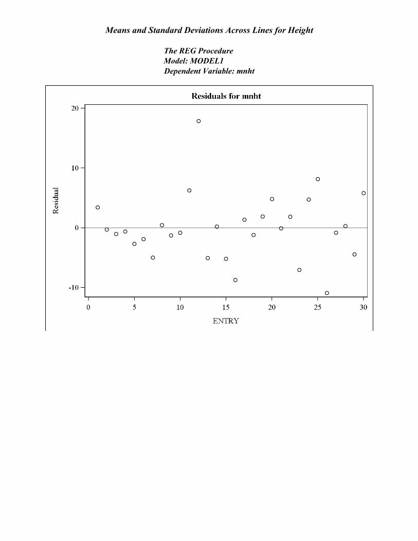
ods graphics on; ods rtf file='residual plot SAS output.rtf'; proc sort; by entry; proc means mean noprint; by entry; var hddt ht lodg yield; output out= new mean=mnhddt mnht mnlodg mnyield varyield; run; proc reg data=new; model mnht =entry/r p influence; title ‘Diagnostics for Simple Linear Regression on Plant Height’;

run; ods rtf close; ods graphics off;

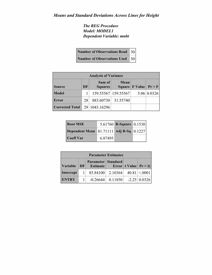
Means and Standard Deviations Across Lines for Height

The REG Procedure Model: MODEL1 Dependent Variable: mnht

Number of Observations Read 30 Number of Observations Used 30

Analysis of Variance

Source DF Sum of

Squares Mean

Square F Value Pr > F

Model 1 159.55567 159.55567 5.06 0.0326 Error 28 883.60730 31.55740 Corrected Total 29 1043.16296

Root MSE 5.61760 R-Square 0.1530 Dependent Mean 81.71111 Adj R-Sq 0.1227 Coeff Var 6.87495

Parameter Estimates

Variable DF Parameter

Estimate Standard

Error t Value Pr > |t|

Intercept 1 85.84100 2.10364 40.81 <.0001 ENTRY 1 -0.26644 0.11850 -2.25 0.0326



Output Statistics

Obs Dependent

Variable Predicted

Value Std Error

Mean Predict Residual Std Error Residual

Student Residual -2-1 0 1 2

Cook's D RStudent

1 89.0000 85.5746 2.0010 3.4254 5.249 0.653 | |* | 0.031 0.6457 2 85.0000 85.3081 1.9002 -0.3081 5.286 -0.0583 | | | 0.000 -0.0572 3 84.0000 85.0417 1.8016 -1.0417 5.321 -0.196 | | | 0.002 -0.1924 4 84.1667 84.7752 1.7055 -0.6086 5.352 -0.114 | | | 0.001 -0.1117 5 81.8333 84.5088 1.6124 -2.6754 5.381 -0.497 | | | 0.011 -0.4904 6 82.3333 84.2423 1.5229 -1.9090 5.407 -0.353 | | | 0.005 -0.3475 7 79.0000 83.9759 1.4375 -4.9759 5.431 -0.916 | *| | 0.029 -0.9136 8 84.1667 83.7094 1.3571 0.4572 5.451 0.0839 | | | 0.000 0.0824 9 82.1667 83.4430 1.2826 -1.2763 5.469 -0.233 | | | 0.001 -0.2294

10 82.3333 83.1766 1.2152 -0.8432 5.485 -0.154 | | | 0.001 -0.1510 11 89.1667 82.9101 1.1560 6.2566 5.497 1.138 | |** | 0.029 1.1444 12 100.5000 82.6437 1.1063 17.8563 5.508 3.242 | |******| 0.212 4.0284 13 77.3333 82.3772 1.0676 -5.0439 5.515 -0.915 | *| | 0.016 -0.9118 14 82.3333 82.1108 1.0409 0.2226 5.520 0.0403 | | | 0.000 0.0396 15 76.6667 81.8443 1.0273 -5.1777 5.523 -0.937 | *| | 0.015 -0.9354 16 72.8333 81.5779 1.0273 -8.7446 5.523 -1.583 | ***| | 0.043 -1.6295 17 82.6667 81.3114 1.0409 1.3552 5.520 0.245 | | | 0.001 0.2413 18 79.8333 81.0450 1.0676 -1.2117 5.515 -0.220 | | | 0.001 -0.2159 19 82.6667 80.7786 1.1063 1.8881 5.508 0.343 | | | 0.002 0.3374 20 85.3333 80.5121 1.1560 4.8212 5.497 0.877 | |* | 0.017 0.8733 21 80.1667 80.2457 1.2152 -0.0790 5.485 -0.0144 | | | 0.000 -0.0141 22 81.8333 79.9792 1.2826 1.8541 5.469 0.339 | | | 0.003 0.3336 23 72.6667 79.7128 1.3571 -7.0461 5.451 -1.293 | **| | 0.052 -1.3089 24 84.1667 79.4463 1.4375 4.7203 5.431 0.869 | |* | 0.026 0.8653 25 87.3333 79.1799 1.5229 8.1534 5.407 1.508 | |*** | 0.090 1.5447 26 68.0000 78.9134 1.6124 -10.9134 5.381 -2.028 | ****| | 0.185 -2.1562 27 77.8333 78.6470 1.7055 -0.8137 5.352 -0.152 | | | 0.001 -0.1493 28 78.6667 78.3806 1.8016 0.2861 5.321 0.0538 | | | 0.000 0.0528



Output Statistics

Obs Dependent

Variable Predicted

Value Std Error



Cook's D RStudent

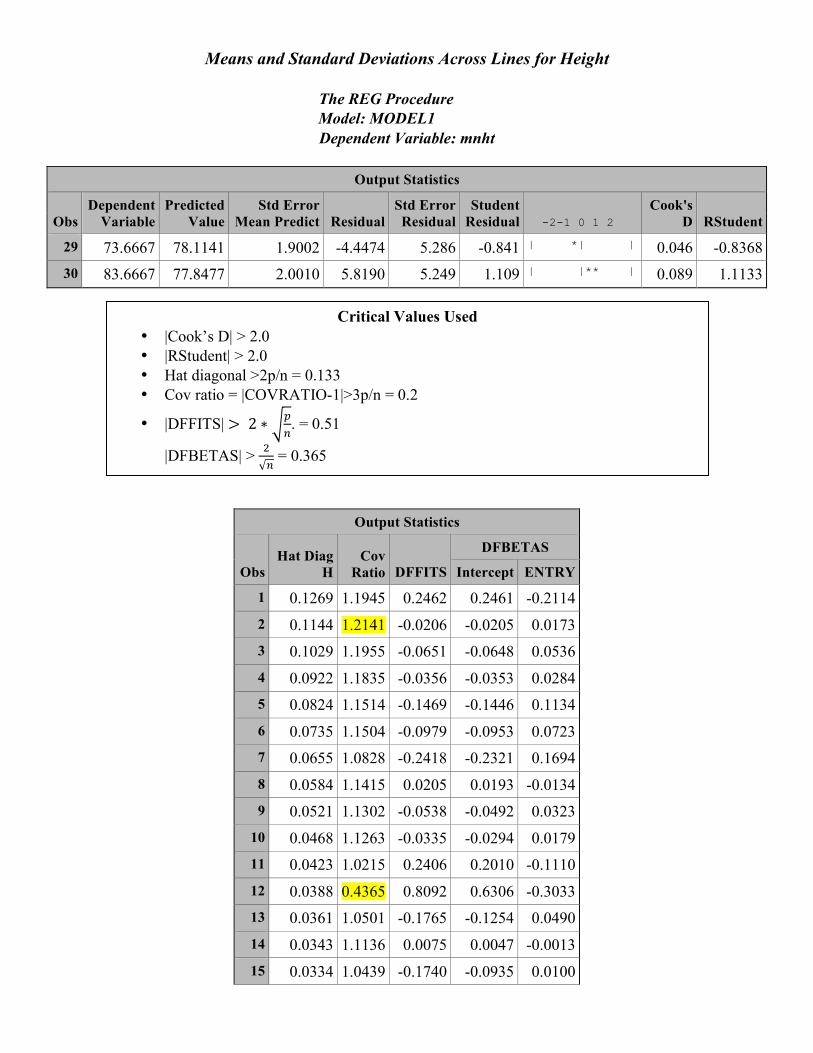
29 73.6667 78.1141 1.9002 -4.4474 5.286 -0.841 | *| | 0.046 -0.8368 30 83.6667 77.8477 2.0010 5.8190 5.249 1.109 | |** | 0.089 1.1133

Output Statistics

Obs Hat Diag

H Cov

Ratio DFFITS

DFBETAS

Intercept ENTRY

1 0.1269 1.1945 0.2462 0.2461 -0.2114 2 0.1144 1.2141 -0.0206 -0.0205 0.0173 3 0.1029 1.1955 -0.0651 -0.0648 0.0536 4 0.0922 1.1835 -0.0356 -0.0353 0.0284 5 0.0824 1.1514 -0.1469 -0.1446 0.1134 6 0.0735 1.1504 -0.0979 -0.0953 0.0723 7 0.0655 1.0828 -0.2418 -0.2321 0.1694 8 0.0584 1.1415 0.0205 0.0193 -0.0134 9 0.0521 1.1302 -0.0538 -0.0492 0.0323

10 0.0468 1.1263 -0.0335 -0.0294 0.0179 11 0.0423 1.0215 0.2406 0.2010 -0.1110 12 0.0388 0.4365 0.8092 0.6306 -0.3033 13 0.0361 1.0501 -0.1765 -0.1254 0.0490 14 0.0343 1.1136 0.0075 0.0047 -0.0013 15 0.0334 1.0439 -0.1740 -0.0935 0.0100

Critical Values Used • |Cook’s D| > 2.0 • |RStudent| > 2.0 • Hat diagonal >2p/n = 0.133 • Cov ratio = |COVRATIO-1|>3p/n = 0.2

• |DFFITS| > 2 ∗ !!!. = 0.51

|DFBETAS| > !√!

= 0.365



Output Statistics

Obs Hat Diag

H Cov

Ratio DFFITS

DFBETAS

Intercept ENTRY

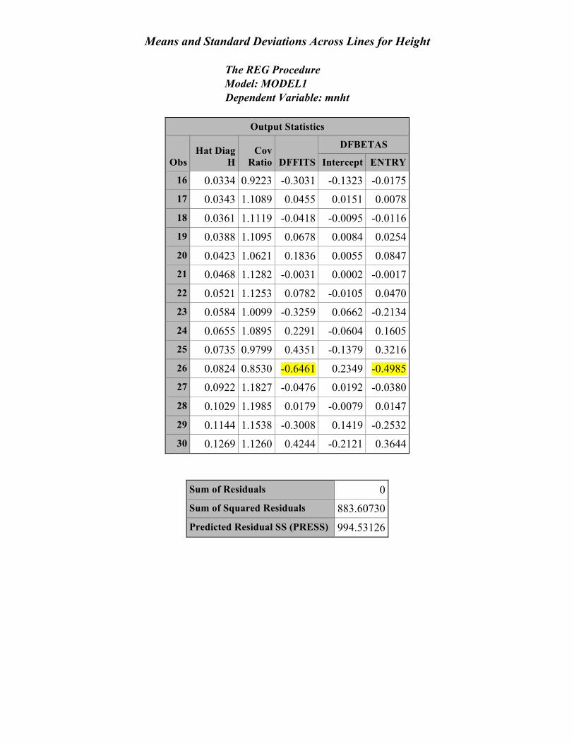
16 0.0334 0.9223 -0.3031 -0.1323 -0.0175 17 0.0343 1.1089 0.0455 0.0151 0.0078 18 0.0361 1.1119 -0.0418 -0.0095 -0.0116 19 0.0388 1.1095 0.0678 0.0084 0.0254 20 0.0423 1.0621 0.1836 0.0055 0.0847 21 0.0468 1.1282 -0.0031 0.0002 -0.0017 22 0.0521 1.1253 0.0782 -0.0105 0.0470 23 0.0584 1.0099 -0.3259 0.0662 -0.2134 24 0.0655 1.0895 0.2291 -0.0604 0.1605 25 0.0735 0.9799 0.4351 -0.1379 0.3216 26 0.0824 0.8530 -0.6461 0.2349 -0.4985 27 0.0922 1.1827 -0.0476 0.0192 -0.0380 28 0.1029 1.1985 0.0179 -0.0079 0.0147 29 0.1144 1.1538 -0.3008 0.1419 -0.2532 30 0.1269 1.1260 0.4244 -0.2121 0.3644

Sum of Residuals 0 Sum of Squared Residuals 883.60730 Predicted Residual SS (PRESS) 994.53126

Example of Using Diagnostics for Multiple Linear Regression options pageno=1; data regdiag; input Line $ Plump Protein Extract amylase DP Kolbach Solprot Color FAN Betagluc Viscosity Fructose Glucose Maltose Maltotriose; datalines; 1 93.75 12.8 77.9 79.2 152.9 47.35 6.06 2.15 309.4 214.4 1.465 0.0945 1.05 4.105 0.99 2 95.1 12.7 76.95 78.95 142.4 50.15 6.36 2.4 380.95 261.95 1.465 0.21 1.08 3.895 0.97 3 95.75 13 77.35 76.95 152.7 48.15 6.24 2.4 318.75 202.05 1.45 0.127 1.04 3.765 0.955 4 94.35 13 78.5 71.2 130.75 51.05 6.655 3.55 307.55 174.4 1.455 0.1535 1.085 3.505 1 5 91.75 12.35 78.7 81.45 158.75 49.05 6.06 2.25 312.9 141.15 1.435 0.1185 1.03 4.155 1 6 92.4 13.1 77.25 63.6 138.55 49.85 6.545 3.6 340.45 124.5 1.47 0.1295 1.16 3.67 1.255 7 95.7 12.8 78.6 64.2 150.9 46.9 5.995 2.15 312.25 142.25 1.445 0.0965 0.935 3.865 1.01 8 91.3 12.7 78.15 60.1 146.05 51.7 6.525 2.55 328.75 176.95 1.455 0.1055 0.92 3.73 0.995 9 90.45 12.2 78.1 60.6 147.55 46.65 5.7 2.05 301 238.15 1.465 0.132 0.95 4.105 1.05 10 91.95 11.8 79.45 77.8 138.4 57.8 6.825 2.75 370.2 140.75 1.48 0.1775 1.275 3.89 1.05 12 93.35 12.9 77.15 64.35 147.75 54.35 7.01 2.55 352.15 197.85 1.475 0.1135 0.995 3.845 0.995 13 90.65 12.05 78.85 62.85 147.05 47.1 5.68 2 273.75 133.5 1.455 0.094 0.915 4.14 0.995 14 96.1 12.95 77.25 76.85 150.25 49.45 6.41 2.2 314.45 260.35 1.45 0.106 1.025 4.04 0.97 15 95.4 13.25 79.7 74 134.05 52.3 6.945 3.75 338 152.3 1.43 0.317 1.22 3.685 1.055 16 89.9 12.85 77.6 58.1 158.05 41 5.275 1.8 290.35 180.2 1.46 0.124 0.905 4.01 0.92 17 96.35 12.55 78.3 62.65 154.6 46.55 5.83 2.1 315.25 234.15 1.455 0.0795 0.965 3.945 0.96 18 95.7 12.9 79.1 75.45 156.25 47.25 6.1 2.25 311.15 150.35 1.415 0.0935 1.03 4.1 0.965 19 92.85 12.75 79.55 60.65 133.65 46.6 5.935 2.5 331.6 152.85 1.435 0.141 1.18 4.01 1.045 21 91.4 12.8 79.7 60.7 140.3 48.9 6.245 3 341.15 161.4 1.45 0.162 1.08 3.67 1.03 22 92.5 12.4 78.7 65.35 120 52.3 6.49 3.65 327.3 207.15 1.485 0.0865 1.155 3.805 1.08

23 94.1 12.8 77.85 72.4 148.85 53.4 6.84 2.35 288.45 225.7 1.455 0.1175 1.05 4.17 0.995 24 93.55 12.85 77.65 66.15 118.3 51.2 6.585 2.85 328.25 219.4 1.48 0.1325 1.165 3.815 1.01 25 94.25 12.6 78.45 69.5 140.85 54.5 6.86 2.35 258.05 219.4 1.475 0.124 1.045 4.16 1.02 26 95.4 12.3 78.55 67.95 132.65 51.45 6.315 2.45 292.25 220.05 1.46 0.1105 0.985 4.11 1.015 27 92.3 12.3 78.6 68.8 128.5 53.35 6.565 2.15 285.4 185 1.445 0.0765 0.975 4.02 0.96 29 92.6 12.3 78.6 71.95 123.35 50.4 6.2 2.05 302.85 160.85 1.475 0.085 1.09 4.16 1 32 91.95 12.15 78.75 73.65 144.65 52.15 6.325 2.4 298.45 178.5 1.47 0.0695 1.03 4.18 1.01 33 92.2 12.2 78.9 68.85 144.35 48.95 5.975 2.35 326.25 171.25 1.465 0.1115 1.03 4.195 0.99 35 96.1 13.45 77.95 66.55 159.7 49.15 6.61 2.3 301.95 182.75 1.475 0.078 0.935 3.91 0.945 36 93.75 12.4 78.25 60.85 121.15 52.1 6.435 3.05 347.25 132.5 1.45 0.1675 1.025 3.855 1.08 37 93.5 12.7 78.6 70.25 120.75 52.85 6.725 3.25 314.55 203.6 1.47 0.123 1.125 3.85 0.975 41 93.25 12.1 78.95 57.7 120.55 52.15 6.32 3.1 333.75 165.65 1.51 0.061 0.98 4.005 1.08 42 92.6 13.2 77.45 72.4 150.05 50 6.595 2.3 362.35 207.55 1.5 0.115 0.995 4.05 0.94 43 92.45 12.35 78.35 68.5 125.7 53.6 6.635 3.65 334.2 134.25 1.5 0.1365 1.14 3.79 1.12 44 92.05 12.95 78.8 61.55 146.7 51.85 6.715 2.25 348.35 178.95 1.46 0.0855 0.95 4.13 0.98 48 90.35 12.65 78.05 59.75 144.2 48.55 6.155 2.2 351.15 155.25 1.47 0.2955 0.96 4.255 1 49 89.35 12.6 78.65 55.95 137.55 55.85 7.015 3.25 346.5 152.5 1.485 0.023 0.98 3.975 1.085 50 89.35 12.2 77.85 58.05 138.5 52.4 6.385 2.15 314.05 157.3 1.46 0.1575 1.015 3.935 1 51 93.6 12.65 78.85 67.9 131.8 49.75 6.37 2.95 282.15 130.15 1.49 0.284 1.13 3.84 0.975 52 92.7 12.6 78.35 60.7 146.25 54.3 6.865 2.55 299.95 192.75 1.455 0.2245 0.935 4.09 0.99 54 95.75 12.5 78.25 72.4 150.35 56.25 7.055 2.65 388.35 176.8 1.47 0.053 0.9 4.025 0.915 56 89.45 12.4 78.85 73.85 147.6 55.35 6.86 2 335.45 161.65 1.475 0.089 0.96 4.125 0.905 58 91.8 12.6 79.35 68.15 162.45 51.25 6.455 2.1 298.15 125.45 1.455 0 1.04 4.27 0.965

60 92 12.1 79.5 66.6 156.35 54.85 6.625 2.1 266.05 155.05 1.425 0 0.925 3.945 0.9 62 89.1 12.35 77.35 58.5 138.55 53.5 6.595 2.7 305.8 137.35 1.47 0 1.055 4.05 1.07 63 91.35 12.4 78.35 64.65 146.55 57.65 7.14 2.6 283 124.4 1.45 0 1.19 4.125 0.905 64 93.6 12.5 78.15 72.05 150.2 49.85 6.235 2.2 301.7 131.3 1.475 0 1.285 4.125 1.015 65 93.25 13.1 77.1 60.45 160.6 49.9 6.54 2.1 327.4 216.4 1.45 0 1.015 4.055 0.955 66 92.55 12.6 78.4 59.8 144.8 48.85 6.18 2.15 287.5 232.9 1.47 0 0.89 4.04 0.965 67 96.55 12.55 78.7 74.8 140.55 55.25 6.915 3.3 346.45 146.6 1.43 0 1.08 4.155 1.03 68 95.3 11.9 77.85 68.5 129.05 54.85 6.53 3.45 406.8 184.5 1.47 0 0.99 4.035 0.89 69 93 12.35 78.25 70.25 133.45 53.15 6.545 3.4 370.3 153.25 1.49 0 1.185 3.93 0.965 70 95.2 12.35 77.5 58.85 142.35 49 6.065 2.65 291.8 163.5 1.485 0 1.015 3.895 0.99 71 91.5 12.3 79.5 71.25 140.5 46 5.62 3.05 360.2 132.2 1.425 0 1.125 3.785 0.95 LACEY 94.9 12.55 78.6 65.8 153.8 48.35 6.065 2.1 290.5 141.75 1.46 0 0.99 4.165 0.955 LEGACY 89.7 12 78.1 76.95 129.55 56.9 6.83 3.65 279.6 149.2 1.505 0 1.19 3.79 1.065 MOREX 91.05 12.6 76.8 66.05 171.4 45.05 5.66 2 333.65 169.65 1.455 0 0.965 4.22 0.68 ROBUST 94.2 12.55 78.25 59.65 143.05 45.1 5.665 2.35 361.1 187.6 1.45 0 0.965 3.97 0.92 STANDER 92.8 11.75 78.6 67 136.9 52.5 6.16 2.9 323.55 173.75 1.455 0 1.18 4.005 0.97 STELLAR 93.45 11.8 78.25 67.95 146.25 40.6 4.835 2.25 281.5 165.4 1.495 0 1.165 4.13 0.95 TRADITIO 95.3 12.45 77.35 71.4 176.2 45.75 5.685 2 291.8 256.35 1.515 0 0.975 4.26 0.905 ;; ods graphics on; ods rtf file='multregdiag.rtf'; proc reg; model extract=betagluc viscosity/p r influence; title 'Data Diagnostics for Multiple Linear Regression'; run; ods graphics off; ods rtf close;

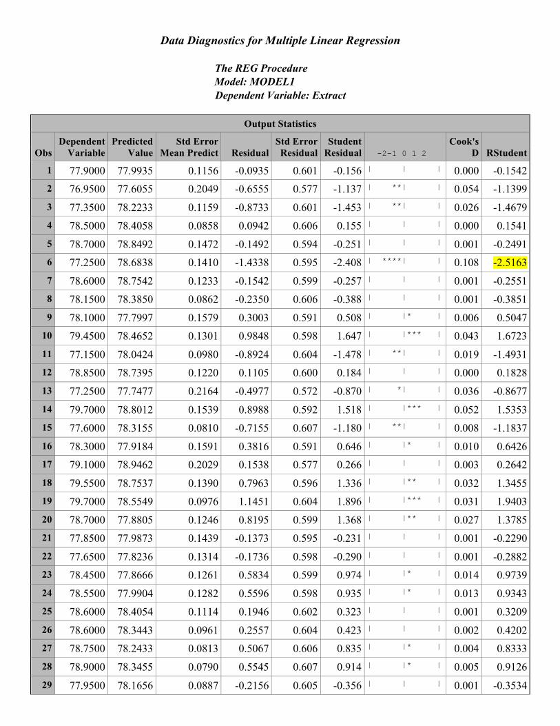
Data Diagnostics for Multiple Linear Regression

The REG Procedure Model: MODEL1 Dependent Variable: Extract

Number of Observations Read 61 Number of Observations Used 61

Analysis of Variance

Source DF Sum of

Squares Mean

Square F Value Pr > F

Model 2 8.23325 4.11663 10.99 <.0001 Error 58 21.71617 0.37442 Corrected Total 60 29.94943

Root MSE 0.61190 R-Square 0.2749 Dependent Mean 78.31721 Adj R-Sq 0.2499 Coeff Var 0.78130

Parameter Estimates

Variable DF Parameter

Estimate Standard

Error t Value Pr > |t|

Intercept 1 92.34866 5.52445 16.72 <.0001 Betagluc 1 -0.00816 0.00219 -3.72 0.0005 Viscosity 1 -8.60486 3.80337 -2.26 0.0274



Output Statistics

Obs Dependent

Variable Predicted

Value Std Error



Cook's D RStudent

1 77.9000 77.9935 0.1156 -0.0935 0.601 -0.156 | | | 0.000 -0.1542 2 76.9500 77.6055 0.2049 -0.6555 0.577 -1.137 | **| | 0.054 -1.1399 3 77.3500 78.2233 0.1159 -0.8733 0.601 -1.453 | **| | 0.026 -1.4679 4 78.5000 78.4058 0.0858 0.0942 0.606 0.155 | | | 0.000 0.1541 5 78.7000 78.8492 0.1472 -0.1492 0.594 -0.251 | | | 0.001 -0.2491 6 77.2500 78.6838 0.1410 -1.4338 0.595 -2.408 | ****| | 0.108 -2.5163 7 78.6000 78.7542 0.1233 -0.1542 0.599 -0.257 | | | 0.001 -0.2551 8 78.1500 78.3850 0.0862 -0.2350 0.606 -0.388 | | | 0.001 -0.3851 9 78.1000 77.7997 0.1579 0.3003 0.591 0.508 | |* | 0.006 0.5047

10 79.4500 78.4652 0.1301 0.9848 0.598 1.647 | |*** | 0.043 1.6723 11 77.1500 78.0424 0.0980 -0.8924 0.604 -1.478 | **| | 0.019 -1.4931 12 78.8500 78.7395 0.1220 0.1105 0.600 0.184 | | | 0.000 0.1828 13 77.2500 77.7477 0.2164 -0.4977 0.572 -0.870 | *| | 0.036 -0.8677 14 79.7000 78.8012 0.1539 0.8988 0.592 1.518 | |*** | 0.052 1.5353 15 77.6000 78.3155 0.0810 -0.7155 0.607 -1.180 | **| | 0.008 -1.1837 16 78.3000 77.9184 0.1591 0.3816 0.591 0.646 | |* | 0.010 0.6426 17 79.1000 78.9462 0.2029 0.1538 0.577 0.266 | | | 0.003 0.2642 18 79.5500 78.7537 0.1390 0.7963 0.596 1.336 | |** | 0.032 1.3455 19 79.7000 78.5549 0.0976 1.1451 0.604 1.896 | |*** | 0.031 1.9403 20 78.7000 77.8805 0.1246 0.8195 0.599 1.368 | |** | 0.027 1.3785 21 77.8500 77.9873 0.1439 -0.1373 0.595 -0.231 | | | 0.001 -0.2290 22 77.6500 77.8236 0.1314 -0.1736 0.598 -0.290 | | | 0.001 -0.2882 23 78.4500 77.8666 0.1261 0.5834 0.599 0.974 | |* | 0.014 0.9739 24 78.5500 77.9904 0.1282 0.5596 0.598 0.935 | |* | 0.013 0.9343 25 78.6000 78.4054 0.1114 0.1946 0.602 0.323 | | | 0.001 0.3209 26 78.6000 78.3443 0.0961 0.2557 0.604 0.423 | | | 0.002 0.4202 27 78.7500 78.2433 0.0813 0.5067 0.606 0.835 | |* | 0.004 0.8333 28 78.9000 78.3455 0.0790 0.5545 0.607 0.914 | |* | 0.005 0.9126 29 77.9500 78.1656 0.0887 -0.2156 0.605 -0.356 | | | 0.001 -0.3534



Output Statistics

Obs Dependent

Variable Predicted

Value Std Error



Cook's D RStudent

30 78.2500 78.7907 0.1282 -0.5407 0.598 -0.904 | *| | 0.012 -0.9022 31 78.6000 78.0385 0.1001 0.5615 0.604 0.930 | |* | 0.008 0.9290 32 78.9500 78.0039 0.1949 0.9461 0.580 1.631 | |*** | 0.100 1.6554 33 77.4500 77.7482 0.1633 -0.2982 0.590 -0.506 | *| | 0.007 -0.5024 34 78.3500 78.3462 0.1911 0.003845 0.581 0.00661 | | | 0.000 0.006557 35 78.8000 78.3257 0.0806 0.4743 0.607 0.782 | |* | 0.004 0.7793 36 78.0500 78.4330 0.0942 -0.3830 0.605 -0.633 | *| | 0.003 -0.6302 37 78.6500 78.3263 0.1269 0.3237 0.599 0.541 | |* | 0.004 0.5374 38 77.8500 78.5023 0.0883 -0.6523 0.605 -1.077 | **| | 0.008 -1.0788 39 78.8500 78.4657 0.1690 0.3843 0.588 0.654 | |* | 0.012 0.6503 40 78.3500 78.2561 0.0960 0.0939 0.604 0.155 | | | 0.000 0.1540 41 78.2500 78.2572 0.0813 -0.007175 0.606 -0.0118 | | | 0.000 -0.0117 42 78.8500 78.3377 0.0954 0.5123 0.604 0.848 | |* | 0.006 0.8454 43 79.3500 78.8052 0.1352 0.5448 0.597 0.913 | |* | 0.014 0.9116 44 79.5000 78.8218 0.1686 0.6782 0.588 1.153 | |** | 0.036 1.1563 45 77.3500 78.5790 0.1191 -1.2290 0.600 -2.048 | ****| | 0.055 -2.1075 46 78.3500 78.8568 0.1408 -0.5068 0.595 -0.851 | *| | 0.013 -0.8489 47 78.1500 78.5853 0.1357 -0.4353 0.597 -0.730 | *| | 0.009 -0.7267 48 77.1000 78.1062 0.1364 -1.0062 0.596 -1.687 | ***| | 0.050 -1.7149 49 78.4000 77.7995 0.1472 0.6005 0.594 1.011 | |** | 0.021 1.0112 50 78.7000 78.8477 0.1570 -0.1477 0.591 -0.250 | | | 0.001 -0.2478 51 77.8500 78.1944 0.0829 -0.3444 0.606 -0.568 | *| | 0.002 -0.5647 52 78.2500 78.2772 0.1398 -0.0272 0.596 -0.0457 | | | 0.000 -0.0453 53 77.5000 78.2366 0.1170 -0.7366 0.601 -1.226 | **| | 0.019 -1.2319 54 79.5000 79.0082 0.1821 0.4918 0.584 0.842 | |* | 0.023 0.8397 55 78.6000 78.6292 0.1073 -0.0292 0.602 -0.0484 | | | 0.000 -0.0480 56 78.1000 78.1812 0.1902 -0.0812 0.582 -0.140 | | | 0.001 -0.1384 57 76.8000 78.4446 0.0861 -1.6446 0.606 -2.715 | *****| | 0.050 -2.8804 58 78.2500 78.3412 0.1011 -0.0912 0.603 -0.151 | | | 0.000 -0.1498



Output Statistics

Obs Dependent

Variable Predicted

Value Std Error



Cook's D RStudent

59 78.6000 78.4111 0.0857 0.1889 0.606 0.312 | | | 0.001 0.3093 60 78.2500 78.1351 0.1452 0.1149 0.594 0.193 | | | 0.001 0.1918 61 77.3500 77.2210 0.2539 0.1290 0.557 0.232 | | | 0.004 0.2298

Output Statistics

Obs Hat Diag

H Cov

Ratio DFFITS

DFBETAS

Intercept Betagluc Viscosity

1 0.0357 1.0912 -0.0297 -0.0014 -0.0218 0.0026 2 0.1122 1.1091 -0.4051 -0.0278 -0.3743 0.0513 3 0.0359 0.9777 -0.2832 -0.1467 -0.1625 0.1541 4 0.0197 1.0733 0.0218 0.0092 0.0007 -0.0089 5 0.0579 1.1146 -0.0617 -0.0444 0.0245 0.0419 6 0.0531 0.8112 -0.5959 0.1266 0.4869 -0.1639 7 0.0406 1.0944 -0.0525 -0.0290 0.0263 0.0265 8 0.0198 1.0665 -0.0548 -0.0232 -0.0054 0.0227 9 0.0666 1.1137 0.1348 0.0083 0.1170 -0.0154

10 0.0452 0.9557 0.3638 -0.1816 -0.2387 0.1997 11 0.0257 0.9637 -0.2423 0.0879 -0.1060 -0.0826 12 0.0398 1.0953 0.0372 0.0087 -0.0265 -0.0065 13 0.1251 1.1577 -0.3281 -0.1072 -0.2948 0.1250 14 0.0633 0.9960 0.3991 0.3289 -0.0808 -0.3178 15 0.0175 0.9970 -0.1581 -0.0354 -0.0250 0.0347 16 0.0676 1.1058 0.1731 0.0511 0.1458 -0.0595 17 0.1099 1.1793 0.0929 0.0840 -0.0123 -0.0819 18 0.0516 1.0114 0.3138 0.2439 -0.0741 -0.2343 19 0.0254 0.8923 0.3135 0.1691 -0.0729 -0.1592 20 0.0415 0.9961 0.2867 -0.1652 0.1324 0.1573 21 0.0553 1.1121 -0.0554 -0.0175 -0.0445 0.0200 22 0.0461 1.0997 -0.0633 0.0244 -0.0421 -0.0218



Output Statistics

Obs Hat Diag

H Cov

Ratio DFFITS

DFBETAS


23 0.0425 1.0471 0.2051 -0.0514 0.1467 0.0427 24 0.0439 1.0528 0.2003 0.0397 0.1565 -0.0485 25 0.0331 1.0838 0.0594 0.0405 0.0171 -0.0408 26 0.0247 1.0702 0.0668 -0.0294 -0.0266 0.0318 27 0.0177 1.0342 0.1117 -0.0276 0.0045 0.0286 28 0.0167 1.0258 0.1188 -0.0037 -0.0146 0.0063 29 0.0210 1.0691 -0.0518 0.0224 -0.0057 -0.0224 30 0.0439 1.0560 -0.1933 -0.0714 0.1299 0.0602 31 0.0267 1.0348 0.1540 -0.0239 0.0898 0.0192 32 0.1015 1.0185 0.5564 -0.4972 -0.1369 0.5058 33 0.0712 1.1194 -0.1391 0.1096 -0.0424 -0.1067 34 0.0976 1.1675 0.0022 -0.0016 -0.0013 0.0017 35 0.0173 1.0386 0.1035 0.0230 0.0129 -0.0223 36 0.0237 1.0569 -0.0982 0.0254 0.0498 -0.0298 37 0.0430 1.0844 0.1140 -0.0734 -0.0560 0.0777 38 0.0208 1.0127 -0.1573 -0.0249 0.0668 0.0181 39 0.0763 1.1156 0.1869 -0.1159 -0.1265 0.1249 40 0.0246 1.0788 0.0245 0.0100 0.0110 -0.0104 41 0.0176 1.0725 -0.0016 0.0004 0.0000 -0.0004 42 0.0243 1.0402 0.1335 -0.0590 -0.0512 0.0636 43 0.0488 1.0605 0.2065 0.0414 -0.1596 -0.0284 44 0.0759 1.0635 0.3314 0.2877 -0.0437 -0.2802 45 0.0379 0.8743 -0.4181 0.0970 0.3056 -0.1212 46 0.0529 1.0713 -0.2007 -0.0654 0.1481 0.0531 47 0.0492 1.0778 -0.1653 0.0581 0.1257 -0.0676 48 0.0497 0.9534 -0.3923 -0.1802 -0.2818 0.1951 49 0.0578 1.0601 0.2506 -0.0173 0.2089 0.0046 50 0.0658 1.1241 -0.0658 -0.0527 0.0183 0.0506



Output Statistics

Obs Hat Diag

H Cov

Ratio DFFITS

DFBETAS


51 0.0184 1.0555 -0.0772 0.0177 -0.0153 -0.0175 52 0.0522 1.1115 -0.0106 0.0076 0.0048 -0.0080 53 0.0365 1.0106 -0.2399 0.1636 0.0785 -0.1700 54 0.0886 1.1141 0.2618 0.2044 -0.1040 -0.1939 55 0.0308 1.0869 -0.0086 -0.0009 0.0057 0.0004 56 0.0966 1.1651 -0.0453 0.0377 0.0193 -0.0389 57 0.0198 0.7150 -0.4092 -0.1673 0.0356 0.1583 58 0.0273 1.0819 -0.0251 -0.0143 -0.0086 0.0145 59 0.0196 1.0693 0.0438 0.0183 0.0008 -0.0177 60 0.0563 1.1143 0.0468 -0.0379 -0.0129 0.0388 61 0.1722 1.2692 0.1048 -0.0729 0.0612 0.0686

Sum of Residuals 0 Sum of Squared Residuals 21.71617 Predicted Residual SS (PRESS) 23.82577

Critical Values Used • |Cook’s D| > 2.0 • |RStudent| > 2.0 • Hat diagonal >2p/n = 0.098 • Cov ratio = |COVRATIO-1|>3p/n = 0.148

• |DFFITS| > 2 ∗ !!!. = 0.444

• |DFBETAS| > !√!

= 0.256


The REG Procedure Model: MODEL1

02:51 Tuesday, June 10, 2014 7


The REG Procedure Model: MODEL1

02:51 Tuesday, June 10, 2014 8

data diagnostics for introduction - ndsu · data diagnostics for introduction ... source df sum of...

Documents