Data dissemination in wireless computing environments

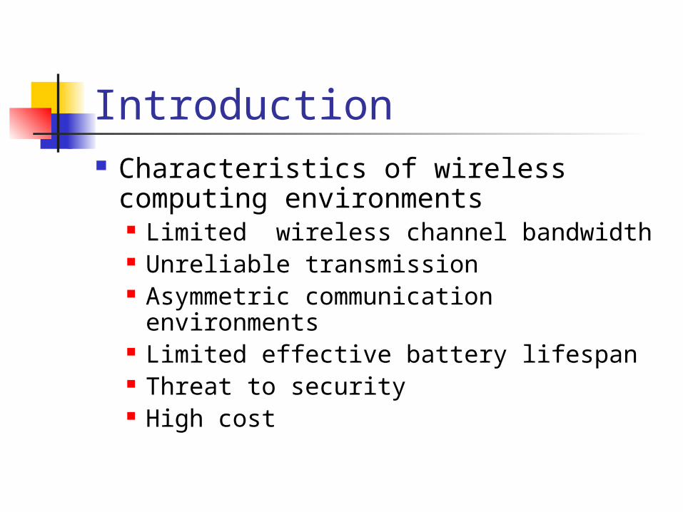
Introduction Characteristics of wireless

computing environments Limited wireless channel bandwidth Unreliable transmission Asymmetric communication

environments Limited effective battery lifespan Threat to security High cost

Design issues in wireless data dissemination Efficient wireless bandwidth utilization Efficient and effective scheduling

strategies at the server Energy-efficient data access for

battery-powered portable devices Support for disconnection Support for secured and reliable

transmission

Models for information dissemination Point to point Push-based Pull-based Hybrid

Static dynamic

Data broadcast scheduling Organization of broadcast for push-

based broadcast system Access time Tuning time Broadcast program

Flat program Skewed non-flat program Regular non-flat program

Broadcast cycle

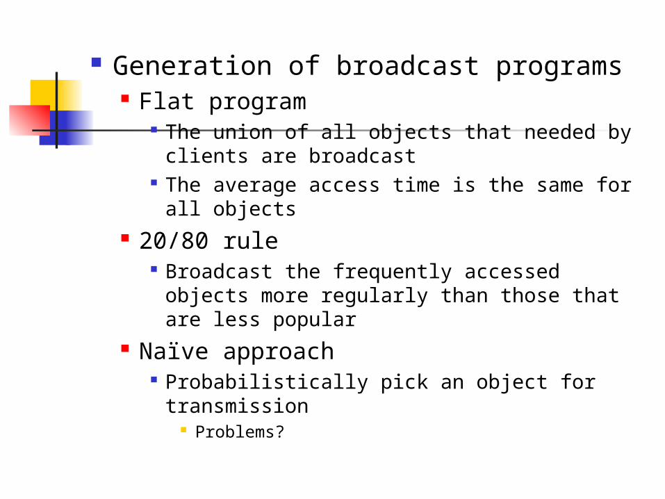
Generation of broadcast programs Flat program

The union of all objects that needed by clients are broadcast

The average access time is the same for all objects

20/80 rule Broadcast the frequently accessed objects

more regularly than those that are less popular

Naïve approach Probabilistically pick an object for

transmission Problems?

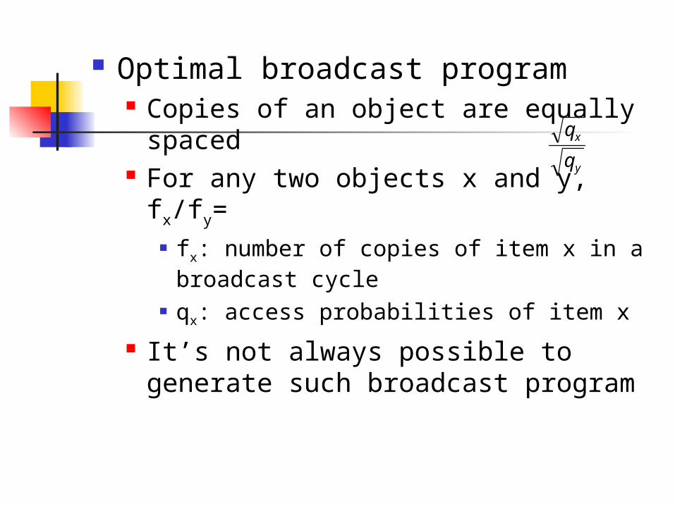
Optimal broadcast program Copies of an object are equally

spaced For any two objects x and y, fx/fy=

fx: number of copies of item x in a broadcast cycle

qx: access probabilities of item x

It’s not always possible to generate such broadcast program

y

x

q

q

Broadcast disk Data is split into n partitions Data with similar access frequency is put

in the same partition Partitions with larger access frequencies

will be broadcast more often than those with smaller access frequencies

Scheduling strategies for pull-based broadcast system Methods

FCFS LWF MRF R*W

Performance metrics Responsiveness Scheduling overhead Robustness Fairness

Indexing on air Basic protocol for retrieving

broadcast data

Flat broadcast programs with indexes (1,m) index

A complete index is broadcast m times during a bcast

All buckets have an offset to the beginning of the next index segment

discussion High average access time Good tuning time

Consideration Is it need to replicate the complete index between

successive data blocks?

Tree-based index A data file is associated with a B+ tree

index structure Broadcast media is a sequential medium,

the data file and index must be flattened Preorder traversal

First k levels of the index will be partially replicated in the broadcast, and the remaining levels will not be replicated

All non-replicated buckets contain pointers that will direct the search to the next copy of its replicated ancestors

Hash-based index Data are hashed into a set of partitions

Partitions may have different sizes (nonuniform distribution)

Hpartition(k) : determines the partition that that object k belong to

Hhash: determines the hash bucket that contains the shift pointer

The gap between hash buckets is given by the size of the smallest partition

Hhash = 1+(hpartition-1)*gap

Signature-based index Signature

An abstraction of the information stored in an object or a file

K-levels of signature The higher the level is, the coarser the granularity of

the grouping is Each integrated signature is broadcast before

the corresponding group of objects. To reduce the number of false drops, the

hashing functions used in generating the signatures at different levels should be different.

Flexible indexing scheme Split a sorted list of objects into several

equal-sized segments At the beginning of each segment, there is a

control index Global index Local index

Discussion

Broadcast program generation for skewed data access Access frequencies can be exploited

to design index methods that further minimize the average number of index probes

Two kinds of approach Imbalanced tree approach Non-flat broadcast programs with indexes

Non-flat broadcast programs with indexes

Segment-level index Similar to the (1,m) index scheme Broadcast a full index at the beginning of each

segment The broadcast program is generated under

broadcast disks Problems

The cost to find the index may be very large

Distributed indexing Each segment index is split into sub-indexes

that are distributed within its corresponding segment

Broadcast Data Allocation for Multiple Data Items Access in Mobile Environments

Broadcast-based query processing model Database Broadcasting

Database partition problem Query processing and data allocation

problem

Cost metrics of query processing for the broadcast data Access time

The time elapsed from the moment a client first tune in the broadcast channel to the moment all the relevant data are downloaded

Tuning time The time spent by the client listening to

the broadcast channel, which is an indicator of the power consumption.

Tuple-based partition The data object on the channel is the

tuple.

Attribute-based partition The data object on the channel is the

atomic value.

Example

Assume there are three relations relation A = (a1, a2, a3)

relation B = (b1, b2, b3)

relation C = (c1, c2)

How to process the following query

Select a2, b2

From A, B

Where a1 < 20 and a1 = b1

Query processing Offline process

The query processing is performed after the values for all the relevant attributes are downloaded.

The tuning time is fixed for a query. The access time is dependent on the order of

attributes on the broadcast channel.

Online process The query processing is performed during the

access of the values for each relevant attribute. The tuning time is minimal, if the access order

of attributes is followed as the process order of query optimization.

Broadcast Model for Off-line Query Processing

Problem formulation The server needs to schedule the data

objects of the queries on the broadcast channel to minimize the average access time

The measure Query Distance (QD) [CK99] is used to show the coherence degree of a query’s QDS in a schedule.

Total Query Distance(TQD) The summation of QD(Qi)*freq(Qi) of all queries Represent the average access time under the

corresponding schedule

Definition of QD Suppose QDS(Qi) is {d1,d2,…,dn}, and i is

the interval between di and di+1 in schedule . Then the QD of Qi on is defined as: QD(Qi,)= BC –MAX( j) where BC is the length of a broadcast cycle.

Example schedule = {d1, d2, d3, d4, d5, d6, d7, d8,

d9, d10} There is a query Qt and its Query Data

Set(QDS) is {d2, d4, d5, d8}. Then the QD of Qt is 10-3=7 in this schedule.

Broadcast Model for Off-line Query Processing

Data scheduling issues Allocate the co-access data close to each other

to reduce the average access time Query-Oriented Approach

Query Expansion Method (QEM) [CK99] Policy 1: Higher-frequency queries have higher

precedence for expansion. Policy 2: During expanding the QDS of a query,

the QD of the queries which had been previously expanded, remain unchanged.

Policy 3: When expanding query qi into the current schedule, the proposed method always minimizes the QD of qi as much as possible.

Example freq(Q1)=100, freq(Q2)=80, freq(Q3)=50 current schedule = [ d2, d3, d4, d6 ] expand Q2

Left-append = [ d5, d7 ] [ d3, d4 ] [ d2, d6 ] expand Q3

Left-append = [ d1 ] [ d5, d7 ] [ d3, d4 ] [ d2, d6 ]

TQD = 100*(7-3)+80*(7-3)+50*(7-3)=920 d1 2d

d

dd

dd

3

4

5

6

7

Q2

Q3 Q1

Modified query expansion method Allow changing the QD of the previously expanded

queries

Change_QD = [ d5, d7 ] [ d4 ] [ d2, d6 ] [ d3 ] [ d1 ] TQD=100*(7-3)+80*5+50*2=900

(a) (b)

(c)

(d)

The condition of applying the moving operation

Example freq(Q3)=50 < freq(Q4)+freq(Q5)=30+25=55 TQD of applying the moving operation

900+30*(7-3)+25*(7-3)=1120 TQD of not applying the moving operation

920+30*(7-5)+25*(7-5)=1030

))()(()(& )()(

))()(()(& )()(

)()()(

ccQj

cj

ccQi

ciQOverlapQDSQQDS

QOverlapQQDSj

QOverlapQDSQQDSQOverlapQQDS

ic QfreqQfreqQfreq

Data-Oriented Approach the content of broadcast schedule are expanded data item by

data item Construct Data access graph

1.      make each data item di as a vertex.

2.      for each query Qi QC

3.      for any two data items di and dj in QDS(Qi)

4.      if edge (di, dj) does not exist

5.      add an edge between vertices di and dj.

6.      set w(di, dj) = freq(Qi).

7.      else8.     set w(di, dj) = w(di, dj) + freq(Qi).

Vertices combination

Combination order with the larger Weighted Distance is selected.

))()()((

),(,

)()()(length

),(wmax(

vu,Distance

vandu between j)(i, egdes jorderiorderulengthBC

jiw

jorderiorderu

ji

Weighted

all

Broadcast Model for On-line Query Processing

Query processing The tuning time is minimal, if the

access order of attributes is followed as the process order of query optimization

Query pattern [SA,JA,PA] Structure of the channel

Flow of query processing Example

SchemaData

Attributea1

SchemaData

Attributeb1

Attributea2

Attributeb2

Attributea3

Attributeb3

Attributec1

Attributec2

1. Tune in the broadcast channel and look for the nearest schema data. Extract all thetuples from the schema data which are corresponding to the attributes in SA, JA andPA.

2. Initially, put all TupleNos into the list relevant_tuple.

3. If SA is not empty, enter the doze mode to wait for the next incoming attribute in SA.Retrieve all the values for that attribute with their TupleNos in the list relevant_tuple.Perform the corresponding query processing and update the list relevant_tuple.Continue this step until all attributes in SA are processed.

4. If JA is not empty, perform the process similar to Step 3. A join operation isperformed until all relevant attributes have been downloaded.

5. Perform the process similar to Step 3 for the attributes in PA. No extra queryprocessing is performed here. Finally, we integrate the relevant values into the finalquery result.

Broadcast Model for On-line Query Processing Preliminary concepts

Access graph Directed weighted graph Represent the relationship among the

data objects Given an access graph G(V,E), the

optimal broadcast order is the order with minimum average access time

1

0

))())(/)((()/1(b

k Eeji

Eeijij

ij ij

rkewewb

data object i data object j

ri->jfirsti

lastj

broadcast cycle n

data object j data object i

lastj

b

firsti

broadcast cycle n+1

data object j data object i

ri->j

Broadcast Model for On-line Query Processing

Optimal cycle ordering problem Given an access graph G(V, E), the problem

is to find a one-to-one function f: V{1, 2, 3, ..., |V|} such that

(denoted as costcycle ) is minimized, where

The Optimal Cycle Order (OCO) of the

access graph is the optimal broadcast order of the access graph.

Ee

jiij

ij

rew )(

bbfirstlastr ijji mod)(

Broadcast Model for On-line Query Processing

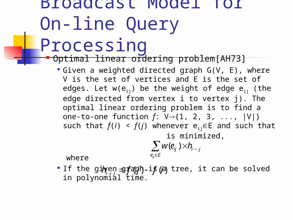
Optimal linear ordering problem[AH73] Given a weighted directed graph G(V, E), where V is

the set of vertices and E is the set of edges. Let w(eij) be the weight of edge eij (the edge directed from vertex i to vertex j). The optimal linear ordering problem is to find a one-to-one function f: V{1, 2, 3, ..., |V|} such that f(i) < f(j) whenever eijE and such that is minimized,

where If the given graph is a tree, it can be solved in

polynomial time.

Ee

jiij

ij

hew )(

)()( ifjfh ji

Broadcast Model for On-line Query Processing

Relation between optimal cycle ordering problem and optimal linear ordering problem

If the access graph is a tree, the OCO of the access graph is the same as the Optimal Linear Order (OLO) of the access graph.

How to transform the access graph into an access forest which keep as much information as possible

Maximum branching algorithm[TS92]

Broadcast Model for On-line Query Processing Represent query patterns as an

access graph Decomposition law

[a,b,c,d] => [a,b], [b,c], [c,d] Cancellation law

[a,b] with access frequency 50, [b,a] with access frequency 30

[a,b] with access frequency 20

How to transform a set of query patterns into an access graph

Example Query pattern1=[{a,f}, {b,c}, {d,e}] with access

frequency f1= 20, query pattern2 =[{c}, {a,d}, {b,e,g}] with Access frequency f2=30

Known access order [a, b], [a, c], [f, b], [f, c], [b, d], [b, e], [c, d],

[c, e] and all with access frequency 20 [c, a], [c, d], [a, b], [a, e], [a, g], [d, b], [d, e],

[d, g], and all with access frequency 30 Merge these two set of access sequence2

[f, b], [f, c], [b, e], [c, e] with access frequency 20

[a, e], [d, e], [a, g], [d, g] with access frequency 30

[a, b], [c, d] with access frequency 20+30 [c, a], [d, b] with access frequency 30-20

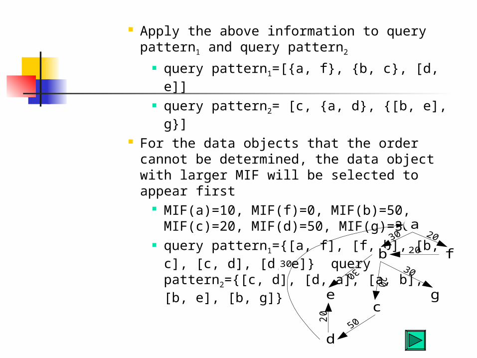
Apply the above information to query pattern1 and query pattern2

query pattern1=[{a, f}, {b, c}, [d, e]] query pattern2= [c, {a, d}, {[b, e], g}]

For the data objects that the order cannot be determined, the data object with larger MIF will be selected to appear first

MIF(a)=10, MIF(f)=0, MIF(b)=50, MIF(c)=20, MIF(d)=50, MIF(g)=30

query pattern1={[a, f], [f, b], [b, c], [c, d], [d, e]} query pattern2={[c, d], [d, a], [a, b], [b, e], [b, g]}

a

b f

c

d

e g

20

20

30

condition above thesatisfied x][y, no is thereif 0,

circuit)any in containednot is

x][y, andx before appearingobject data any denotes y wherex] [y,

ofset theamongfrequency maximum the| ( :

:)(

maxmax ff

xMIF

b c

50

30

20

20

Broadcast Model for On-line Query Processing The scheduling algorithm

Example of transforming an access graph into an access forest

e

d a

k

l j

i

m

h

g

fcb

2

4

2

5

35

4

3

3

4 5 3

7

4 72

e

d a

cbf

k

l m

h

gj

i

7

There are three cases of information loss can be considered

Refining the access graph to avoid the information loss

Re-ordering the vertices (a->d) Merging the OLO’s of the access trees (m-

>i) Flow of our approach

access graphrefined access

graphaccess forest

broadcasting orderfor each accesss tree

refining maximumbranching

scheduling

broadcasting orderfor the access graphmerging

The ’ graph can be modified to avoid information loss

Examples

x

r

em2

size 3

size 2 size 4

refine

x

r

em9

size 3

size 2 size 4

refine

size 1

x

r

em2

size 3

size 2 size 1

x

r

em

size 3

size 2

k

l m

h

g

Tree YTree X

e

d a

cbf8

Tree Z

j

i

7

e

d a

k

l j

i

m

h

g

fcb

2

83

Scheduling access tree Based on the optimal linear ordering

algorithm with a consideration of the remove edges where the starting and ending vertices are in the access tree

Re-ordering method The order of the nodes indicated by the

removed edge is the same as the order given by the optimal linear ordering algorithm

The order given by the optimal linear ordering algorithm is different from the direction indicated by the removed edge.

e

a c

cbb

d

d

d

e

e

a c

cbb

30

d

d

d

e

e

a c

cbb

40

d

d

d

ea..c..b.. a..b..c..

Tree XOrder:"edfabc"

e

d a

cbf8

k

l m

h

g

Tree YOrder:"gkhlm"

Tree ZOrder:"ji"

j

i

7

Merging access trees

ZX

Ysize 5

size 2size 6

YZX: gkhlmjiedfabc

Optimal Index and Data Allocation in Multiple Broadcast Channels

Introduction Data Broadcast

advantage: independent of the number of users

disadvantage: sequential access Current Research on Data Broadcast

determining the data for broadcasting scheduling the data broadcasting indexing the broadcast data

Introduction (cont’d.) Index Techniques with Access Patterns

balanced index tree with data replication skewed index tree without data

replication Cost Metric for the Indexing Schemes

access time: response time probe wait: for the first index data wait: for the desired data item

tuning time: listening time

Motivation Skewed Index Tree Allocation

preorder / postorder: single channel level by level: multiple channels

A 4

32

1

DC

EB

20 10

15 7

18

C 1

C 2

1 1 1 1 1 1 1 1

2 3 2 3 2 3 2 3

4 4 4 4 4 4 4 4C 3

Time

Motivation (cont’d.) Level_by_Level Approach [SV96]

lack of flexibility waste of channel space

C 1

C 2

1 1 1 1 1 1 1 1

2 2 2 2 2 2 2 2

3 3 3 3 3 3 3 3C 3

T im e

3

2

1

A

Problem Description Index and Data Allocation (IDA) Problem

given: broadcast channel: C = {C1, C2, C3, ..., Ck} channel slots: S = {S1, S2, S3, ...} index nodes: I = {I1, I2, I3, ..., Im} data nodes: D = {D1, D2, D3, ..., Dn}, weight: W(Di)

allocation: one-to-one mapping a child node is broadcast after a parent node

SCDIf :

Problem Description (cont’d.) Example: One Channel Allocation

A 4

32

1

DC

EB

20 10

15 7

18

01691082067515318

waitdataaverage

701 .)(

C 11 3 E 4 C D 2 A B

35

68

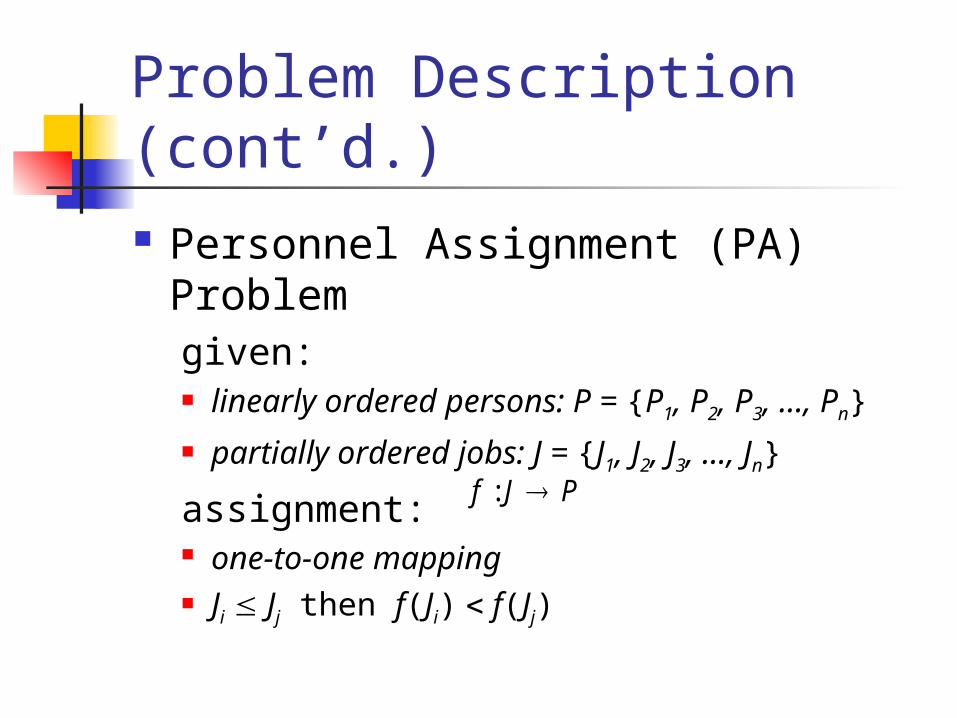
Problem Description (cont’d.) Personnel Assignment (PA) Problem

given: linearly ordered persons: P = {P1, P2, P3, ...,

Pn} partially ordered jobs: J = {J1, J2, J3, ..., Jn}

assignment: one-to-one mapping Ji Jj then f(Ji) f(Jj)

PJf :

Problem Description (cont’d.) Example: Job Assignment

J1P1, J2P2, J3P3, J4P4

J1P1, J2P2, J4P3, J3P4

J 1

J 3

J 2

J 4

Problem Description (cont’d.) IDA ==> PA

J = I D P = S

one channel:

two channels:

S 1 S 2 S 3 S 4 S 5 S 6 S 7 S 8

P 1 P 2 P 3 P 4 P 5 P 6 P 7 P 8C 1

S 1 S 2 S 3 S 4 S 5 S 6 S 7 S 8

C 1

C 2

P 1 P 2 P 3 P 4 P 5 P 6 P 7 P 8

Pruning Algorithm Solution Space Representation

topological tree

J 1

J 3

J 2

J 4

J 1

J 3J 4

J 4J 3

J 2

J 3

J 1

J 3J 4

J 4J 3

J 4J 1

J 2

Person Assigned

P 1

P 2

P 3

P 4

Pruning Algorithm (cont’d.) k-channel Topological Tree

4E

CD

BC

DE

CE

BD

CD

BE

CD

BE

BD

CE

DE

BC

B4

CD

DE

AC

CE

AD

AE

CD

AE

CD

CE

AD

DE

AC

CD

A4

CD

AB

AC

BD

BC

AD

BC

AD

BD

AC

AB

CD

AB

A4

AE

B4

BE

4E

23

1A 4

32

1

DC

EB

20 10

15 7

18

4E

CD

BC

DE

CE

BD

CD

BE

CD

BE

BD

CE

DE

BC

B4

CD

DE

AC

CE

AD

AE

CD

AE

CD

CE

AD

AB

A4

AE

B4

23

1

Pruning Algorithm (cont’d.) Optimal Path ==> Optimal

Allocation

C 1 1 2 A 4 C 1 2 A 4

3 B E D 3 B EC 2

Pruning Algorithm (cont’d.) Pruning Rule

eliminate impossible next_neighbors

AB

A4

AE

B4

BE

4E

23

1

next_neighbors

Pruning Algorithm (cont’d.) Pruning by Swapping

given two neighboring nodes (X is before Y)X = {x1, x2, …, xn}, Y = {y1, y2, …, ym}

global swap:{y1, y2, …, ym}{x1, x2, …, xn}

local swap: {y1, x2, …, xn}{x1, y2, …, ym}

two swapped nodes (elements) no parent-child relationship

Property 1. If index nodes have been all allocated, remaining data nodes have one allocation only

B

1

2

3

A

C

CD

DC

CE

EC

DE

D

ED

4

E

W(C) = 15

W(D) = 7

W(E) = 18

W(E) > W(C) > W(D)prune

Property 2. The next_neighbor of a node with a single index node should be a child of the index node: either an index node or the data node with the largest weight

1

2 3

A B 3 prune

Children(2) = {A, B}, W(A) > W(B)

75

Property 3. Every data node in the next_neighbors of X must be a child of an index node in X, if its weight is larger than that of a data node in X

4E

CD

BC

DE

CE

BD

CD

BE

CD

BE

BD

CE

DE

BC

B4

CD

DE

AC

CE

AD

AE

CD

AD

CE

CD

AE

AB

A4

AE

B4

23

1

X

prune

Pruning Algorithm (cont’d.) Data Tree for 1-Channel

Topological Tree

B

1

2

E4

D

B

C

D

C

4B

D

B

E

C

D

4

C

D

E

E

C

4

3

3

A

4

A

D

C

D

B

B C

D

B

E

D

C

D

E

EC

ECB

Pruning Algorithm (cont’d.) Pruning by Swapping the Data

Nodes

two swapped subsequences S and T

T

Ty

S

Sx

N

yW

N

xW

T

nodedata a is yand

nodedata a isx and

)()(

if S

A

D

E

C

BB

1

2

4

D

E

C

3

A

10/1

15/3

Heuristic Approaches Limit of the Pruning Algorithm

not suitable for a large index tree Two heuristics

index tree sorting: the preorder traversal generates the single channel allocation

index tree shrinking: node combination / tree partition

Heuristic Approaches (cont’d.) Example: Tree Sorting

A 4

32

1

DC

EB

20 10

15 7

18

A4

32

1

DC

EB

20 10

15 7

18

30/3 40/5

22/3 18/1

B

BSubtreey

A

ASubtreex

N

yW

N

xW

nodedata a is yand )(

nodedata a isx and )(

)()(

if BA

Heuristic Approaches (cont’d.) Sorting Performance: O(Nlog m)

4-nary balanced tree with depth 3 access frequency: N(100, )

9.5

10

10.5

11

11.5

12

10 20 30 40 (Variance)

Dat

a W

ait (

buck

ets)

OptimalSorting

Index and Data Allocation on Multiple Broadcast Channels Considering Data Access Frequencies

The Multiple Broadcast Segment-Based Method Basic idea

Extend the work of distributed indexing to the multiple channels environment

Consider the problem of data replication

Distributed indexing All data items are associated with an index

tree The index tree consists of two parts

Replicated index part Non-replicated index partR

a1 a3a2

b1 b3b2 b4 b6b5 b7 b9b8

c6c1 c2 c3 c4 c5 c9c7 c8 c12c10 c11 c15c13 c14 c18c16 c17 c21c19 c20 c24c22 c23 c27c25 c26

1 4 7 10 13 16 19 7976737067646158555249464340373431282522DataItems

ReplicatedIndex Part

Non-replicatedIndex Part

Broadcast program generation Definition

Bi: The ith index node in NRR

Rep(Bi): The sequence of index nodes along the path from the root of the index tree to the non-replicated root Bi (excluding Bi).

Ind(Bi): The index nodes of the index tree rooted at Bi.

Data(Bi): The set of data items indexed by Bi.

Let NRR = {B1, B2, …, Bt}. The broadcast program for the index tree is a sequence of triples:

< Rep(Bi), Ind(Bi), Data(Bi) > Bi NRR, in the left to right order.

Each triple forms a broadcast segment(BS)1 4 7 10 13 16R a1 b1 c1 c2 c3 R a1 b2 c4 c5 c6 R a1 b3 c7 c8 c9 19 2522

28 31 34 37 40 43R a2 b4 c10 c11 c12 R a2 b5 c13 c14 c15 R a2 b6 c16 c17 c18 46 5249

55 58 61 64 67 70R a3 b7 c19 c20 c21 R a3 b8 c22 c23 c24 R a3 b9 c25 c26 c27 73 7976

BS(1) BS(2) BS(3)

BS(4) BS(5) BS(6)

BS(7) BS(8) BS(9)

Extend distributed indexing into multiple channels Generating initial broadcast programs

Sort the sequence of triples < Rep(Bi), Ind(Bi), Data(Bi) > in descending order according to the value of Sum(Bi).

Allocate the triples by the order in each channel. Repeat the allocation until all triples are broadcast

in the channels Example

Assume the number of channels is 3 the order of the summations of access

frequencies is BS(1) > BS(4) > BS(7) > BS(2) > BS(5) > BS(8) > BS(3) > BS(6) > BS(9)

1 4 7 10 13 16R a1 b1 c1 c2 c3 R a1 b2 c4 c5 c6 R a1 b3 c7 c8 c9 19 2522

28 31 34 37 40 43a2 b4 c10 c11 c12 a2 b5 c13 c14 c15 a2 b6 c16 c17 c18 46 5249

55 58 61 64 67 70a3 b7 c19 c20 c21 a3 b8 c22 c23 c24 a3 b9 c25 c26 c27 73 7976

MBS(1) MBS(2) MBS(3)

Refining initial broadcast programs Replication of MBS

Basic idea Broadcast data items with higher access

frequencies more frequently Property 1 [Wong88]

For fixed sized data items, the total average access time will be minimized if the instances of each data item are equally spaced and for any two data items di and dj, where pi is the reciprocal of si which is the probability that di will be selected to broadcast in each time slot, and fi is the access frequency of di

Method Compute M_SUM(i) =

Allocate the MBS(i) according to Property 1 )()(

)(iMBSjBS

jSum

jiji ffpp //

Example Assume that the summation of access

frequencies in MBS(1) is 0.5 and the summation of access frequencies in MBS(2) and MBS(3) are 0.25.

1 4 7 10 13 16R a1 b1 c1 c2 c3 R a1 b2 c4 c5 c6

R a1 b3 c7 c8 c9 19 2522

28 31 34 37 40 43a2 b4 c10 c11 c12 a2 b5 c13 c14 c15

a2 b6 c16 c17 c18 46 5249

55 58 61 64 67 70a3 b7 c19 c20 c21 a3 b8 c22 c23 c24

a3 b9 c25 c26 c27 73 7976

1 4 7R a1 b1 c1 c2 c3

28 31 34a2 b4 c10 c11 c12

55 58 61a3 b7 c19 c20 c21

Data allocation in an MBS Basic idea

Consider the allocation of the index nodes in Ind(Bi) and data items in Data(Bi) to further reduce the average access time for all data items

Method Compute the summation of the access

frequencies of the data items contained in the sub-tree in Ind(Bi)

The sub-trees with higher summations of access frequencies will be allocated first

Example Assume the summations of access

frequencies of data items indexed by c1, c2 and c3 are 0.25, 0.15 and 0.2 respectively

......

Bi

1 47R a1 b1 c1 c2c3

Performance Evaluation Compared approach [LC00]

A 4

32

1

DC

EB

20 10

15 7

18

C1 1 2 A E C 1 2 A E

3 B 4 D 3 B 4C2

C11 2 A B 3 E 4 C D

Effect of the number of nodes Our approach outperforms the other

for the average access time The average tuning time for the two

approaches is almost the same

(a)The average access time (b) The tuning time

0

200

400

600

800

1000

0 500 1000 1500 2000 2500Niumber of data nodes

Ave

rage

acc

ess

tim

e

LC00

Our approach

0

2

4

6

8

10

0 500 1000 1500 2000 2500Number of data nodes

Tuni

ng ti

me

LC00

Our approach

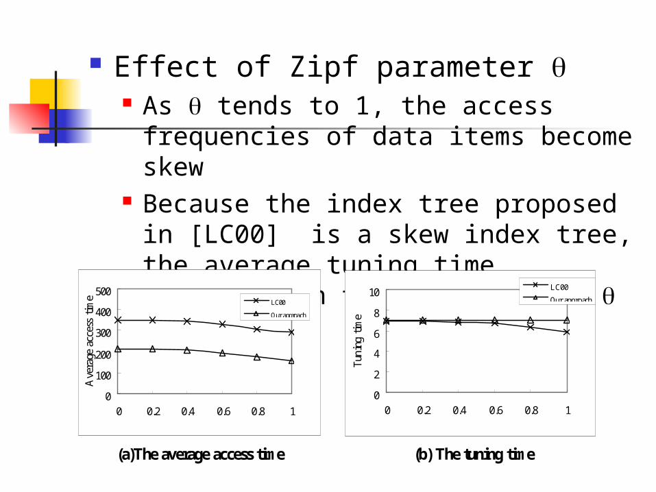
Effect of Zipf parameter As tends to 1, the access

frequencies of data items become skew

Because the index tree proposed in [LC00] is a skew index tree, the average tuning time decreases in this approach as tends to 1

(a)The average access time (b) The tuning time

0

100

200

300

400

500

0 0.2 0.4 0.6 0.8 1

Ave

rage

acc

ess

time LC00

Our approach

0

2

4

6

8

10

0 0.2 0.4 0.6 0.8 1

Tuni

ng ti

me

LC00

Our approach

Effect of the ratio of the size of a data item to the size of an index node In our approach, the data items and index

nodes are allocated in different time slots. The approach proposed in [LC00] mixes the

data items and index nodes in the same time slot.

As the size of data items is greater than the size of index nodes, some broadcast bandwidth allocated to index nodes is wasteful.

(a)The average access time (b) The tuning time

0

300

600

900

1200

1 2 3 4 5Ratio

Ave

rage

acc

ess

tim

e

LC00

Our approach

5

6

7

8

1 2 3 4 5Ratio

Tuni

ng ti

me

LC00

Our approach