data-driven based analog beam selection for hybrid...
TRANSCRIPT

1
Data-driven Based Analog Beam Selection forHybrid Beamforming under Mm-Wave ChannelsYin Long, Zhi Chen, Senior Member, IEEE, Jun Fang, Member, IEEE, Chintha Tellambura, Fellow, IEEE
Abstract—Hybrid beamforming is a promising low-cost solu-tion for large multiple-input multiple-output (MIMO) systems,where the base station (BS) is equipped with fewer radiofrequency chains. In these systems, the selection of codewordsfor analog beamforming is essential to optimize the uplink sum-rate. In this paper, based on machine learning, we proposea data-driven method of analog beam selection to achieve anear-optimal sum-rate with low complexity, which is highlydependent on training data. Specifically, we take the beamselection problem as a multiclass-classification problem, wherethe training data set consists of a large number of samples of themillimeter-wave channel. Using this training data, we exploit thesupport vector machine (SVM) algorithm to obtain a statisticalclassification model, which maximizes the sum rate. For real-timetransmissions, with the derived classification model, we can select,with low complexity, the optimal analog beam of each user. Wealso propose a novel method to determine the optimal parameterof Gaussian kernel function via McLaughlin expansion. Analysisand simulation results reveal that, as long as the training datais sufficient, the proposed data-driven method achieves a near-optimal sum-rate performance, while the complexity reducesby several orders of magnitude, compared to the conventionalmethod.
Index Terms—hybrid beamforming, data-driven solution, mm-wave, beam selection, SVM
I. INTRODUCTION
Although the fifth generation (5G) mobile communicationsstandards are still very much evolving, the aims for higher datarates, lower latency, and higher energy-efficient performanceare firmly clear [1]. These aims bring about the demands forwider bandwidth spectrum. Currently, available bandwidth inthe spectrum up through 6 GHz is not sufficient to satisfythese requirements. This shortage, in turn, has helped us movethe target operating frequency bands up into the millimeter-wave (mm-wave) [2] range for the next generation of wirelesscommunication systems [3] [4]. The shorter wavelengths atthese higher frequency bands enable implementations withmany more antenna elements per system within a super-small space [5] [6]. However, it also increases the signal-path and propagation challenges associated with operating at
This work was supported in part by the Important National Science andTechnology Specific Projects of China under Grant 2017ZX03001010, and bythe Science and Technology on Communication Networks Laboratory fund.
Yin Long is with Science and Technology on Communication NetworksLaboratory, University of Electronic Science and Technology of China,China, e-mail: ([email protected]); Zhi Chen and Jun Fang are withNational Key Lab of Science and Technology on Communications, Uni-versity of Electronic Science and Technology of China, China, e-mail:([email protected]); ([email protected]); Chintha Tellambura is withDepartment of Electrical and Computer Engineering, University of Alberta,Canada, e-mail: ([email protected])
these frequencies. For example, due to the gas absorption, theattenuation for a 60 GHz waveform is more than 10 dB/km,while a 700 MHz waveform experiences an attenuation on theorder of 0.01 dB/km.
These losses can be compensated with the elaborate arraydesign and the application of spatial signal-processing tech-niques, including beamforming. Beamforming can be enabledby large antenna arrays and can be applied directly to providehigher transmit gains to cope with the path loss and harmfulinterference signals.
To achieve a desirable flexibility and controllability withbeamforming in the design of antenna array, adopting anindependent weighting control over each antenna-array ele-ment is a feasible method. This requires a transmit or receivecomponent dedicated to each antenna-array element. However,for large multiple-input multiple-output (MIMO) systems [7][8] whose array size is over a hundred antennas, such anarchitecture is rather difficult to build due to cost, space,and power limitations. For example, implementing a highperformance analog-to-digital converter (ADC) and digital-to-analog converter (DAC) for each channel can drive the cost andpower beyond an affordable budget. Similarly, having variablegain amplifiers in the radio frequency (RF) chain for eachchannel can increase system cost.
Hybrid beamforming [9] [10] [11] is a popular techniquethat can be used to partition beamforming into digital domainand RF domain. Therefore, hybrid beamforming can be imple-mented to balance tradeoffs between cost and flexibility, whilestill fielding a system that meets the required performanceparameters. Hybrid-beamforming designs are developed bycombining multiple array elements into subarray modules.A transmit or receive module can be dedicated to multipleelements in the array. Thus, the system will need fewertransmit or receive components (i.e., RF chains). The numberof elements in each subarray can be selected to ensure thatsystem performance is met across the range of steering angles.Using the transmit path as an example, each element withina subarray can have a phase shift applied directly in theRF domain, while digital beamforming techniques based oncomplex weighting vectors can be applied on the signals thatfeed each subarray. Digital beamforming is able to conductthe control of the signal for both amplitude and phase onsignals aggregated at the subarray level. Consequently, a cost-efficient MIMO system architecture for low-cost deploymentis proposed, which is called hybrid MIMO.
In hybrid beamforming, each RF chain is equipped witha bunch of phase shifters to conduct analog beamforming.Thus, to ensure a high performance in terms of sum-rate or bit
2
error rate for hybrid MIMO, choosing suitable analog beamsfor each RF chain plays a key role. Thus, recently, a plentyof works have focused on the selection of analog beams. In[12], a low-complexity analog beam selection scheme underpoint-to-point scenarios is proposed. When the number ofcandidates of analog beams is small, the proposed schemeis able to achieve a near-optimal spectral efficiency at highSNR regime. Literature [13] presents two beam selectionalgorithms for analog beamforming based on rotman lenstheory, which is able to achieve higher BER performance. In[14], an exhaustive method is proposed to select the analogbeams that make SNR or SINR maximum. However, so far,all the related works try to find the optimal combination ofanalog beams by evaluating the design metric over all possiblecombinations. Nevertheless, evaluating the design metric is ahigh-complexity task, thus choosing suitable analog beams foreach RF chain is a high complexity-cost procedure, whichposes an unacceptable delay on real-time communications.Therefore, developing a low-complexity method is motivated.
Recently, big data [15] [16], which is an emerging technol-ogy about extracting meaningful value from large volume ofdata, has attracted a plenty of interests in various fields. Bigdata enables us to harness the volume, variety, and velocity ofdata and deduce actionable insight from data. In the study ofcellular networks, big data would bring us huge opportunitiesto innovate cellular networks, since big data is able to providenovel efficient solutions to the design or optimization ofcellular networks. For example, cellular networks embracingbig data have been studied in [17]. A self-optimizing 5Gnetworking based on big data is proposed in [18]. Furthermore,as mentioned in [17] and [18], machine learning [19] is apowerful tool in big data, which is able to dig hidden insightsfrom training data and make a judgment for a new data set.
In this paper, to solve the analog beam selection problemin a low-complexity way, we propose a data-driven solutionby resorting to support vector machine (SVM) [20]. SVM is apreferred multi-class classification algorithm [21] in machinelearning, which is good at handling linearly inseparable datasetof samples and avoiding over-fitting. To begin with, we con-sider the beam selection problem as a multi-class classificationproblem, where a large number of samples of mm-wavechannel are taken as training data. Based on these training data,we adopt SVM algorithm to obtain a statistical classificationmodel in terms of maximizing sum-rate performance. Byusing the derived classification model, we can choose theoptimal analog beam for each user with low complexity inthe middle of real-time transmission. Analysis and simulationresults reveal that, if training data can be provided sufficiently,the proposed data-driven method is able to achieve a near-optimal sum-rate performance, while the complexity wouldreduce by several orders of magnitude, compared with theconventional exhaustive method.
To the best of our knowledge, this paper is the first attemptto solve the problem of beam selection by the data-drivenmethod. Our main contributions are as follows:
1) As we know, directly calculating sum-rate for zero-forcing (ZF) digital beamformer is involved with severalmatrix inversion operations, which is a high-complexity
manipulation. Thus, in this paper, by using the vector-combined manipulation, we derive a low-complexity met-ric to measure sum-rate. Moreover, we take the derivedmetric as the key performance indicator (KPI) of eachpossible combination of analog beams.
2) In machine learning, training data is presented as featurevector whose dimensionality is proportional to the com-plexity of classification. In order to reduce the complexityof classification, we take the direction of arrival (DoA)and angle Of arrival (AoA) of each path of mm-wavechannels as entries of feature vectors. Due to the sparsityof mm-wave channels [22], the number of transmissionpath of mm-wave channels is few. Hence, the dimension-ality of feature vector of training data is very small, whichis able to suppress the complexity of classification.
3) Generally, in hybrid beamforming, a codebook of analogbeams provides more than two candidates for beamsselection, which brings about the imbalance of trainingdata for an one-vs-the-rest classifier [20]. However, theregular SVM does not perform well on imbalanced data.Therefore, we propose a biased-SVM where the majortraining data and minor training data use different errorpenalty, respectively.
4) The classification performance of SVM primarily de-pends on the design parameter of kernel functions. Toachieve a high classification performance, we propose anew method to determine the optimal design parameter ofthe Gaussian kernel function in virtue of McLaughlin ex-pansion. The experiment results indicate that the proposedmethod can achieve a better classification performancethan conventional cross-validation method.
The reminder of this paper is organised as follows. InSection II, we introduce the system model. In Section III, alow-complexity metric for sum-rate is obtained. In Section IV,a data-driven solution for analog beam selection is proposed.In Section V, the complexity analysis is conducted. Simulationresults are presented in Section VI. Finally, the paper issummarized in Section VII.
Notations: x, x and X denote scalar, vector and ma-trix, respectively. xT represents the transpose of vector x.diag[x1, x2, · · · , xk] denotes a matrix whose diagonal ele-ments are composed by x1, x2, · · · , xk while the rest ofelements are zero. ∥·∥ represents Forbinius norm. S denotesa set, and |S| is the cardinality of set S.
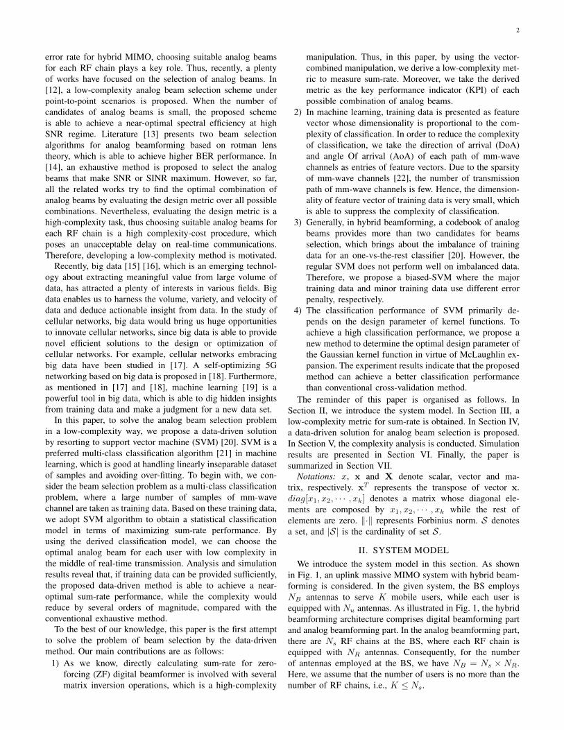
II. SYSTEM MODELWe introduce the system model in this section. As shown
in Fig. 1, an uplink massive MIMO system with hybrid beam-forming is considered. In the given system, the BS employsNB antennas to serve K mobile users, while each user isequipped with Nu antennas. As illustrated in Fig. 1, the hybridbeamforming architecture comprises digital beamforming partand analog beamforming part. In the analog beamforming part,there are Ns RF chains at the BS, where each RF chain isequipped with NR antennas. Consequently, for the numberof antennas employed at the BS, we have NB = Ns × NR.Here, we assume that the number of users is no more than thenumber of RF chains, i.e., K ≤ Ns.
3
ADC
DAC
DBF
ADC
ADC
RF
RF
RF
RF
RF DAC
User 1
User K
Fig. 1. System model
A. Analog beamforming
Basically, as we know, analog beamforming is aim to adjustthe phase of the transmitted or received signal at antennas inthe RF domain by using phase shifters in front of each antenna.
To begin with, we assume only a single data stream needsto be transmitted for each user. Hence, when the kth (k ∈1, 2, · · · ,K) user transmits uplink signal to the BS throughan analog beam, the uplink signal of the kth user can be writtenas
xk = cksk (1)
where sk ∈ C1×1 is the data symbol of the kth user, ck ∈CNu×1 is the analog beam for the kth user, and the ith entryof ck is the value of phase shift on the ith antenna, denoted byejθ
ki with θki ∈ [0, 2π]. For each user, the maximum transmit
power of the uplink signal is P , namely, E[∥xk∥2
]≤ P .
Then, the received data steams at the BS is expressed by
y =
K∑i=1
Hixi + n =
K∑i=1
Hicisi + n (2)
where Hi ∈ CNB×Nu is the uplink channel matrix of user i,and n ∼ CN (0, INB
) represents the additive white Gaussiannoise (AWGN) at the BS.
On the other hand, the receive phase shifter vector for thelth RF chain of the BS can be given by
gl =[ejθ
l1 , · · · , ejθ
lNR
]T(3)
where the ith entry of gl, ejθli , is the value of phase shifter on
ith antenna of the lth RF chain. Hence, based on the systemmodel mentioned above, the receive phase shifter matrix at theBS, G, can be written as a Ns × NB block diagonal matrixwhich is consisted of the Ns receive phase shifter vectors andcan be expressed as
G =
gT1 0 · · · 00 gT
1 · · · 0...
.... . .
...0 0 · · · gT
Ns
. (4)
Then, after being processed by the receive phase shifter
matrix, the received signal can be given by
y = GK∑i=1
Hixi +Gn =K∑i=1
GHicisi +Gn
=K∑i=1
hisi +Gn
=[h1h2 · · · hK
]
s1s2...sK
+Gn
= Hs+Gn
(5)
where hi∆=GHici is the equivalent channel vector for the
uplink channel of the ith user and H∆=[h1, h2, · · · hK
].
B. Digital beamformingIn the baseband process, the ZF beamforming is considered
to detect the each user’s uplink signal. Based on the criterionof ZF, the receive digital-beamforming matrix is the pseudoinverse of H, which is given by
W =((
H)H
H)−1(
H)H
. (6)The detected signal by using ZF beamforming can be ex-pressed as
y = Wy =((
H)H
H)−1(
H)H
y
=
s1s2...sK
+((
H)H
H)−1(
H)H
Gn.(7)
C. Mm-wave ChannelAlthough hybrid beamforming is able to be operated in
Rayleigh fading conditions, we need to adopt the mm-wavefrequency band due to the demands for wider bandwidthspectrum. Hence, in this paper, we adopt the most widelyapplicable geometric channel models. As a mm-wave channelmodel, the geometric channel model has L limited scatteringpath. Consequently, the uplink channel of user k, Hk, can bewritten as
Hk =
√NBNu
Lρk
L∑i=1
αk,iaBS(θBSk,i )a
Huser(θ
userk,i ) (8)
where αk,i is the complex gain of the ith path with E [|αk,i|] =1, ρk is the path loss between the BS and the kth user andthe variables θuserk,i ∈ [0, 2π] and θBS
k,i ∈ [0, 2π] are the AoDsof user k and AoAs of the BS of the ith path, respectively.Regardless of the elevation, we consider the azimuth only,which implies that both BS and users conduct horizontalbeamforming only. Consequently, aHuser(θ
userk,i ) and aBS(θ
BSk,i )
are the antenna array response vectors at the user and theBS, respectively. Here, we adopt uniform linear arrays. Thus,aHuser(θ
userk,i ) and aBS(θ
BSk,i ) can be written as
auser(θuserk,i )
=1√NB
[1, ej2πλ d sin(θuser
k,i ), · · · ej(Nu−1) 2πλ d sin(θuser
k,i )],(9)
aBS(θBSk,i )
=1√NB
[1, ej2πλ d sin(θBS
k,i ), · · · ej(NB−1) 2πλ d sin(θBS
k,i )],(10)
4
respectively, where λ is the signal wavelength and d is thedistance between antenna elements. The channel model in (8)can be written in a more compact form as
Hk = ABSdiag(b)AHuser (11)
where b =√
NBNu
Lρk[αk,1, αk,2, · · · , αk,L]. The matrices
Auser and ABS contain the user and the BS array responsevectors, respectively, which are given byAuser = [auser(θ
userk,1 ),auser(θ
userk,2 ), · · ·auser(θuserk,L )], (12)
ABS = [auser(θBSk,1 ),auser(θ
BSk,2 ), · · ·auser(θBS
k,L)]. (13)
The channel model in (8) turns out to be Rayleigh fadingchannel when L is very large. Based on the channel stateinformation, the BS selects the analog beams for both the BSand users.
Note that: Since channel estimation is beyond the scope ofthis study, we consider that the parameters of the L channelpaths, such as AoA, AoD, and the complex gain of each path,can be estimated perfectly and known to the BS.
D. Analog beam set
We assume each user chooses a transmit analog beam from acodebook F which is a set consisted of |F| predefined analogbeams. The predefined codecook of transmit analog beams canbe represented as
F =c1, c2, · · · c|F|
(14)
where ci ∈ CNu×1 (i ∈ 1, 2, · · · , |F|) is a possible optionof the transmit analog beam for a given user. The nth entryof ci is ejθ
in which is the value of phase shift on the corre-
sponding antenna for a given user. Similarly, the predefinedcodecook of receive analog beams can be represented as
G =G1,G2, · · ·G|G|
(15)
where Gm ∈ CNS×NB (m ∈ 1, 2, · · · , |G|) is a possibleoption of the receive analog beam for the BS.
If the kth user takes cn as the transmit analog beam, basedon (5), the equivalent uplink channel vector for the kth usercan be expressed as
hn,mk = GmHkc
n. (16)Here, we assume that each user shares a same predefinedcodecook of transmit analog beams, which is known to theBS.
E. Uplink Sum-rate
Based on (7), the sum-rate of the uplink MIMO system canbe given by
R =
K∑i=1
log2(1 + γi) (17)
where γi is the signal-to-interference-plus-noise ratio (SINR)of ith user and can be written as [23] [24]
γi =P
NuNRσ2
[((H)H
H)−1
]i,i
. (18)
According to (17) and (18), it is worth noting that theSINR of the ith user is dependent on the equivalent channel.Based on the definition of the the equivalent channel, we knowthat the equivalent channel is involved with analog beams.
Therefore, each user needs to select an optimal analog beamfrom the predefined codecook of transmit analog beams tomaximize the uplink sum-rate. Specifically, the optimizationproblem of analog beam selection can be formulated as
G, c1, c2 · · · cK= max
G∈G,ci∈F
K∑i=1
log2(1 + γi). (19)
Intuitively, we can obtain an optimal solution for the aboveproblem by exhaustive search, such as [12] and [14]. How-ever, the exhaustive search makes the complexity rather high,especially when the number of antennas or the number ofcandidates beams is very large. Hence, it is very meaningfulto develop a low-complexity method to solve this problem. Inthe following subsection, we discuss a sub-optimal solutionfor analog-beam selection.
III. SUB-OPTIMAL SOLUTION FOR ANALOG-BEAMSELECTION
To begin with, we know that, directly calculating SINR (18)for ZF digital beamforming is involved with matrix inversionoperation which is a high-complexity manipulation. Thus, weneed to derive a low-complexity metric to measure sum-rate.
A. Novel metric for sum-rateFirstly, we conduct an analysis of sum-rate under a special
case where K = 2. And then, we would expand the analysis togeneral multi-user cases. According to (18), the uplink sum-rate under K = 2 can be given as
R =2∑
i=1
log2
(1 +
P det(h1, h2
)NuNRσ2
∥∥hi
∥∥2)
(20)
where i = 1, 2 /i anddet(h1, h2
)=∥∥h1
∥∥2∥∥h2
∥∥2 − (h1
)Hh2
(h2
)Hh1. (21)
Proof: See Appendix A.By resorting to some math manipulations, (20) can be
rewritten asR = log2
(1 + Pf
(h1, h2
))(22)
where
f(h1, h2
)=
det(h1h2)
NuNRσ2∥∥h1
∥∥2 +det(h1h2)
NuNRσ2∥∥h2
∥∥2+
P(det(h1h2)
)2N2
u(NR)2σ4∥∥h1
∥∥2∥∥h2
∥∥2 .(23)
Due to the logarithmic function in (22), a positive corre-lation exists between the uplink sum-rate R and f
(h1, h2
).
Therefore, we consider the function f(h1, h2
)as an evalu-
ating metric to select an optimal analog beam for each user,which would derive the optimum solution for maximizing theuplink sum-rate in a low-complexity way.
In order to generalize the metric to the general case whereK ≥ 3, we are able to combine K − 1 equivalent channelvectors into a new equivalent channel vector. Specifically, theevaluating metric can be written as f
(hk, hk
)where k is the
complementary set of k, hk
is the (K−1)-combined equivalentchannel vector and can be written as
hk =∑i∈k
aiGmHici (24)
with ai being the normalized coefficient.Thus, the multi-user case is turned into a two-user case.

5
B. Sub-optimal solution
According to the metric derived above, the details of theanalog beam selection algorithm would be presented in thefollowing.
1) To begin with, we fix the receive analog beam by choos-ing one of beams in G as receive analog beam. Then, werepresent the set of users who have already chosen analogbeams by S, while denote the set of users who have notchosen analog beams by Ω. Then, compute the Forbiniusnorm of equivalent channel vectors for each combinationof |F| transmit analog beams and K users, then we findout the pair of user and beam which can obtain themaximum Forbinius norm among K |F| combinations.This procedure can be expressed as
(i, ci) = arg max(k∈Ω,cn∈F)
∥∥hn,mk
∥∥2. (25)
2) Compute the combined channel vector over the equivalentchannel vectors of users from set S. This procedure canbe expressed as
h =∑i∈S
aiGmHici (26)
where ai = GmHici/∑
i∈S GmHici is the weightedfactor of the ith user whose optimal analog beam is xi.Similarly, this procedure can be formulated as
(i, ci) = arg max(k∈Ω,cn∈F)
f(h, hn,m
k
). (27)
3) continue the procedures above until the optimal analogbeams of all users under current receive analog beam aredetermined.
4) repeat the procedures above until all receive analog beamsin G are took. And take the analog beam Gm withmaximum value of metric (23) as the optimal receiveanalog beam G.
C. Algorithm procedure
The detailed step of sub-optimization analog beam selectionalgorithm is illustrated in Alg.1.
One may note that, the analog beam selection methoddescribed above avoids searching over all candidates of analogbeams from codebook F . Consequently, the complexity canreduce significantly compared with exhaustive search, as willbe demonstrated in section V.
IV. DATA-DRIVEN ANALOG BEAM SELECTION
Although the sub-optimization method of selecting analogbeam avoids the exhaustive search, it still involves some high-complexity operations, such as Forbenius norm and matrixmultiplication. For reducing the complexity further, in thissection, we adopt machine learning to solve this problem in alow-complexity way. To be more specific, we exploit SVM toclassify the uplink channels of each user to several differenttypes, where each type corresponds to a candidate of analogbeam. SVM is a supervised machine learning algorithm, whichis mostly used in classification problems. Especially, comparedwith other classification algorithms, SVM has advantages onboth handling linearly inseparable set of samples and avoidingover-fitting since the kernel trick is adopt. In SVM algorithm,
Algorithm 1: Suboptimal algorithmInput: Ω = 1, 2, · · · ,K ,S = ∅, m = 1Output: ck, k = 1, 2, · · ·Kstep 1: For all k ∈ Ω
For all cn ∈ Fhnk = GmHkc
n
step 2: i, ci = arg maxk∈Ω,cn∈F
∥∥hn,mk
∥∥2,∀k, ∀nΩ = Ω− i, S = S + i
step 3: calculate h =∑i∈S
aiGmHici based on (29)
step 4: For all k ∈ ΩFor all cn ∈ Ff(h, hn
k )
Step 5: i, ci = arg maxk∈Ω,cn∈F
f(h, hn,m
k ), ∀k, ∀n
Gm = maxk∈Ω
f(h,GmHici)
Ω = Ω− i, S = S + iStep 6: If |Ω| = 0
If m < |G|m = m+ 1, go to step 1;
ElseG = argmax
G∈GG1, G2, · · ·G|G |
Elsego to Step 3.
we represent each data item as a point in n-dimensional space(where n is the dimensionality of feature vectors) with thevalue of each feature being the value of a particular coordinate.Then, we perform classification by finding the separatinghyper-plane which differentiates the two classes very well. Bythe hyper-plane, when a new input data (current channels ofusers) comes up, we can predict the class (optimal analogbeam) of the new input data.
A. Training Samples Set1) Generating Training Samples: In a supervised machine
learning, training data is indispensable for obtaining the clas-sifying criterion. Here, we assume that M channel samplesare generated for training. Based on the model of mm-wavechannel, each channel sample can be presented by 4L + 1real-value features including the path loss, L complex gain ofpaths (including 2L real-value features), L angles of departureof users and L angles of arrival of the BS. To guarantee theeffectiveness of training, the features of each sample shouldbe randomly generated based on their corresponding statisticalcharacter. Furthermore, since high-value feature would bringabout bias, we need to normalize each feature as
elm =elm −Mean(elm)
elmax − elmin
(28)
where elm is the value of the lth feature of the mth sample,Mean(elm) represents the mean of the lth feature of Msamples, elmax donates the maximum value of the lth featureamong M samples, while elmin represents the minimum valueof the lth feature among M samples.
Then each channel sample can be represented as a featurevector tm ∈ R1×(4L+1) consisted of 4L + 1 normalizedfeatures.

6
2) KPI Function: KPI is used to evaluate the objectivemetric, such as BER, SNR and SINR. Based on the analysis inthe above section, for problem (25), we consider
∥∥GmHkci∥∥2
as the KPI.3) Labeling: There are |F| choices of analog beams for
each user, hence we evaluate the KPI for all possible combi-nations of a given sample and all choices of analog beams.And we label the training simple with cn which is able tolet this training sample obtain the maximum KPI. The labelof all training samples can be presented as vector r ∈ R1×M
consisted of the index of optimal analog beam for M trainingsamples.
B. Regular SVM based classifier
For each feature vector tm (m ∈ 1, 2, · · · ,M), wehave its corresponding class-label r[m]. By using the Mlabeled training samples, we are able to develop a multi-classclassifier where the input is the channel feature vector and theoutput is the optimal analog beam which can maximize KPIfor the input channel. Generally, in hybrid beamforming, acodebook of analog beams provides more than two candidatesfor beams selection. Hence, in order to classify |F| classes,we exploit |F| one-vs-the-rest SVM classifiers, each of whichclassifies a channel feature vector into one category or theother categories. Let us take the nth (n ∈ 1, 2, · · · , |F|)classifier as an example, where we classify the sample labeledby n into one category but classify the other samples intoanother category. For the ith sample, we set yi = +1 if thelabel r[i] = n, while set yi = −1 if r[i] = n. And w is thevector consisting of parameters for the separating hyper-plane.In SVM algorithm, the optimization problem of training theseparating hyper-plane of the nth classifier can be formulatedas
minw,b,ζ
1
2wTw + C
M∑i=1
ζi
s.t. yi(wTϕ(ti) + b
)≥ 1− ζi, i = 1, 2, · · · ,M
ζi ≥ 0, i = 1, 2, · · · ,M
(29)
where ϕ is the mapping function by which the sample data tican be mapped into high-dimensional space, b is the threshold,C is the penalty constant, ζi is the value of error caused bymisclassification for sample ti.
However, in our problem, the number of samples labeledby cn is much smaller than that of other categories. Whenfaced with imbalanced datasets where the number of negativeinstances far outnumbers the positive instances, the perfor-mance of regular SVM drops significantly. A popular approachtowards solving these problems is to preprocess the data byoversampling the majority class or undersampling the minorityclass in order to create a balanced dataset. However, by thisapproach, the data structure is destroyed, which results in ainaccurate separating hyper-plane.
C. Biased-SVM based classifier
In this paper, for solving these problems, we propose anapproach which pays more attention to the positive instances.This can be done, for instance, by increasing the penalty
associated with misclassifying the positive class relative tothe negative class. Specifically, we choose two different plentyconstants for positive samples and negative samples, respec-tively. The optimization can be reformulated as
minw,b,ζ
1
2wTw + C+
∑i|yi=+1
ζi + C−∑
i|yi=−1
ζi
s.t. yi(wTϕ(ti) + b
)≥ 1− ζi, i = 1, 2, · · · ,M
ζi ≥ 0, i = 1, 2, · · · ,M(30)
where C+ and C− are the plenty constants for positive samplesand negative samples, respectively.
The Lagrange duality problem of (30) can be written as
minw,b,ζ
1
2
M∑i=1
M∑j=1
aiajyiyjK(ti, tj)−M∑i=1
ai
s.t.N∑i=1
yiai = 0,
0 ≤ ai ≤ C+, yi = +1,
0 ≤ aj ≤ C−, yj = −1,
(31)
where ai and aj are Lagrange multipliers,K(ti, tj)= ⟨ϕ(ti), ϕ(tj)⟩ is the Gaussian radial-basedkernel function and can be further written as
K(ti, tj) = e(−∥ti−tj∥2/(2σ2)) (32)with σ (σ ≤ σ ≤
σ) being the design parameter.In regular SVM, the optimal set of Lagrange multipliers
of optimization problem can be solved by sequential minimaloptimization algorithm (SMO) [25] with the fast and reliableconvergence. SMO is an iterative algorithm for solving theoptimization problem described in (31). SMO can break thisproblem into a series of smallest possible sub-problems, whichare then solved analytically. However, in the proposed SVM,since the constraint conditions of Lagrange multipliers aredifferent with the regular SVM, we need to analyze newconstraint conditions of Lagrange multipliers for SMO al-gorithm. After each iteration of SMO algorithm, the newLagrange multipliers must be within the constraint area. Forexample, in the case where yi = yj , Ci > Cj , a
oldi >
aoldj ,(aoldi − aoldj
)< (Ci − Cj), based on the relationship
aoldi yi + aoldj yj = anewi yi + anewj yj , we have:
if aj < 0,
anewi = aoldi − aoldj
anewj = 0
if 0 < aj < Cj ,
anewi = aianewj = aj
if aj > Cj ,
anewi = Cj + aoldi − aoldj
anewj = Cj
. (33)
D. Parameter Optimization
As shown above, the classification performance of theproposed SVM method primarily depends on the parameterσ of kernel functions and the penalty constant C+ and C−. Inthis subsection, we discuss how to determine the parametersto achieve an optimal classification performance.
1) Parameter σ: Because SVM is a kind of machinelearning method based on the kernel function, the selectionof the corresponding parameter σ would bring about great

7
Constraint conditions of
traditional SMO
Constraint conditions of
proposed method
Fig. 2. Constraint Conditions of Lagrange Multipliers
influences on the generalization performance of SVM. Atpresent, there has been a few researches on the parameterselection for a given kernel. Among them, cross-validation[26] is considered to be more precise, however it needs totrain SVM for many times, which results in high-complexitytasks.
In this paper, we propose a novel method of determining theoptimal σ in according to spatial distance. For obtaining highaccuracy of classification results, we hope the spatial distancebetween samples of same class is smaller, while the spatialdistance between samples of different classes is farther. Thus,we are able to determine the optimal σ based on this criterion.Specifically, the problem of determining the optimal σ can bewritten as
minσ
∥ϕ(ti)− ϕ(tj)∥2, yiyj = 1
maxσ
∥ϕ(ti)− ϕ(tj)∥2, yiyj = −1.(34)
Based on the fact ∥ϕ(ti)− ϕ(tj)∥2 = 2− 2K(ti, tj) whosedetailed proof is given in Appendix B, the problem (34) canbe rewritten as
yiyj ||ϕ(ti)− ϕ(tj)||2 =minσ
[2− 2K (ϕ(ti), ϕ(tj))] , yiyj = 1
maxσ
[−2 + 2K (ϕ(ti), ϕ(tj))] , yiyj = −1.
Therefore, the problem (34) can be reformulated as
maxσ
M∑i=1
i−1∑j=1
yiyjK(ti, tj) = maxσ
M∑i=1
i−1∑j=1
yiyjeτεij (35)
where εij = ∥ti − tj∥2 and τ = −1/2σ2. Now, by using
Mclaughlin expansion [27],∑M
i=1
∑i−1j=1 yiyje
τεij in (35) canbe represented as
M∑i=1
i−1∑j=1
yiyjeτεij =
M∑i=1
i−1∑j=1
yiyj(1 + τεij +1
2τ2ε2ij)
=
M∑i=1
i−1∑j=1
yiyj + τ
M∑i=1
i−1∑j=1
yiyjτεij + τ2M∑i=1
i−1∑j=1
1
2yiyjε
2ij .
(36)
WhenM∑i=1
i−1∑j=1
12yiyjε
2ij < 0, the optimal τ∗ can be deter-
mined as
τ∗ = −M∑i=1
i−1∑j=1
yiyjτεij
/M∑i=1
i−1∑j=1
yiyjε2ij . (37)
WhenM∑i=1
i−1∑j=1
12yiyjε
2ij > 0, the optimal τ∗ can be deter-
mined asτ∗= max
τ=τ ,
τ
L(τ) (38)
where L∆=∑M
i=1
∑i−1j=1 yiyje
τεij .2) Parameter C+ and C−: As mentioned in section IV,
for the accuracy of the separating hyperplane in imbalanceddatasets, we choose the larger penalty constant for positivesamples, while we choose the smaller penalty constant fornegative samples. In this way, as shown in the optimizationproblem (30), the misclassification for the fewer positive classwould result in larger penalty, thereby improving the accuracyof the SVM classifier. Therefore, based on this criterion, weadopt the reciprocal of the number of positive samples andnegative samples as the C+ and C−, respectively.
E. Classifying Stage
When w, b and design parameters are determined, theclassifier of analog beam cn ∈ |F| can be presented as
gn1 (tk) =∑si∈V1
aiyiK(si, tk) + b (39)
where tk is a new feature vector needed to be classified, si isa support vector, V1 is the set of support vectors.
If gn1 (tk) > 0, we consider ∥GHkcn∥2 outperforms∥∥GHkc
i∥∥2, i = n. Thus the optimal beam for user k is cn.
F. Optimization problem (27)
1) Generating Training Samples: In the problem (27), theaim is to find the optimal combination of k and cn in terms ofmaximizing the objective function f
(h, hn,m
k
)whose input
vectors are h and tk. Basically, the combined channel vectorh is also an equivalent channel vector, so it is justified totake the training samples of equivalent channel vector as thetraining samples of h. Since there are M training samples forthe mm-wave channel H and |F| candidate analog beams, weare able to generate M |F| training samples for the combinedchannel vectors h based on (16). Since another input is featurevector tk which has M training samples, thus there are M2 |F|training samples for the input of (27) by combining h andtk. And each training sample is presented as (Ns + 4L+ 1)-dimension feature vector. Similarly, each feature entry shouldbe normalized in case of bias.
2) KPI Function and Labeling: For the problem (27), weset f (a,b) in (23) as KPI, and each training sample islabeled with the reference number of the analog beam whichis able to obtain maximum KPI. Thus, the M2 |F| samples aredivided into |F| classes. Based on the training of SVM, theseparating hyperplane for each class is obtained. Therefore,when a new feature vector comes up, we are able to derivethe optimal analog beam with which the maximum f (a,b)can be obtained.
3) Classifying Stage: Similarly, the classifier of analogbeam cn can be represented as
gn2
([h, tk
])=∑si∈V2
aiyiK(si,[h, tk
])+ b (40)

8
where tk is a new feature vector needed to be classified,[h, tk
]is a vector combined h and tk, si is a support vector,
V2 is the set of support vectors.If gn2
([h, tk
])> 0, the current analog beam cn can
maximize the KPI function f(h, hn,m
k
)for the new feature
vector tk.
G. Algorithm procedure
The detailed step of data-driven analog beam selectionalgorithm is illustrated in Alg.2.
Algorithm 2: Data-driven analog beam selection algorithmInput: Ω = 1, 2, · · · ,K ,S = ∅,
tk, k ∈ Ω, m = 1,w1
cn , b1cn ,w
2cn , b
2cn , ai
Output: ck, k = 1, 2, · · ·KStep 1: For all k ∈ Ω
For all cn ∈ FIf gn1 (tk) > 0ck = cn, k = k + 1, end;
Elsen = n+ 1.
Step 2: i = arg maxk∈Ω
∥∥hn,mk
∥∥2, ∀kΩ = Ω− i, S = S + i
Step 3: calculate h =∑i∈S
ajGmHici based on (25)
Step 4: For all[h, tk
], k ∈ Ω
For all cn ∈ FIf gn2
([h, tk
])> 0
ck = cn, k = k + 1, end;Elsen = n+ 1.
Step 5: i = arg maxk∈Ω
f(h, hn,m
k ), ∀k
Gm = maxk∈Ω
f(h,GmHici)Ω = Ω− i, S = S + i
Step 6: If |Ω| = 0If m < |G|m = m+ 1, go to Step 1;
ElseG = argmax
G∈GG1, G2, · · ·G|G |
Elsego to Step 3.
V. COMPLEXITY ANALYSIS
In this section, we analyze the complexity of the exhaustivesearch, sub-optimization method and data-driven method foranalog beam selection.
A. Exhaustive search
To begin with, we know that complexity of calculatinginversion of a matrix X ∈ Ct×t is O(t3) [28]. Consequently,the complexity of exhaustive search is
O(|G| |F |KK5N4
SN2uNR
). (41)
B. Sub-optimization method
Firstly, we know that the complexity of calculating For-benius norm of a vector x ∈ Ct×1 is O(t) [28]. Sincethere are K users and each user has |F| possible analogbeams, we need to consider K |F| equivalent channels andto find the first user and its corresponding optimal analogbeam which provides the maximum vector norm (25) amongK |F| equivalent channel vectors. And then the complexityof calculating hk = GHktk is N3
SN2uNR. Consequently, the
complexity of (25) is N3SN
2uNRNSK |F|.
Since the analog beams for the other K − 1 users areselected by using the metric in (23) which is involved with twooperations of Forbenius norm for vector and two operationsof inner product for vectors, the complexity of selecting theoptimal analog beams for the other K − 1 users is
O((K − 1) |F|N3
SN2uNR (2NS)
)+O
((K − 2) |F|N3
SN2uNR (2NS)
)· · ·+O
(|F|N3
SN2uNR (2NS)
)= O
((K − 1)K
2|F|N3
SN2uNR (2NS)
).
(42)
Therefore, the complexity for the sub-optimization analogbeam selection algorithm can be estimated as
O(
N3SN
2uNRNSK |F| |G|
+ (K−1)K2 |F|
(N3
SN2uNR2NS |G|
) ) . (43)
C. Data-driven method
In the data-driven method, the algorithm complexity shouldexclude the training complexity of SVM, due to that thetraining stage is performed offline. Hence, only complexityof classifying should be taken into account. Since the kernelfunction requires a Forbenius norm of a feature vector, thisneeds O(N3
SN2uNRK + |V1| (4L+ 1)K |F|).
Since the analog beams for the other K−1 users are selectedby using the metric in (23), the complexity of selecting theanalog beams for the other K − 1 users is
O(
(K − 1) |F| |V2| ((NS + 4L+ 1))+ (K − 1)N3
SN2uNR
)+O
((K − 2) |F| |V2| ((NS + 4L+ 1))+ (K − 2)N3
SN2uNR
)· · ·
+O(|F| |V2| ((NS + 4L+ 1)) +N3
SN2uNR
)= O
((K−1)K
2 |F| |V2| ((NS + 4L+ 1))
+ (K−1)K2 N3
SN2uNR
).
(44)
Therefore, the complexity for the data-driven method canbe estimated as
O
(N3
SN2uNRK + |V1| (4L+ 1)K |F|
)|G|
+ (K−1)K2 (|F| |V2| (NS + 4L+ 1)) |G|
+ (K−1)K2
(N3
SN2uNR
)|G|
. (45)
Since the poor scattering nature of the mm-wave channel,the number of scattering path L is rather few. On the otherside, the number of support vectors, i.e., |V1|, |V2|, is very few.Thus, the complexity of data-driven method (45) can reducedramatically, compared with sub-optimization method (43).
Remark 1. Similar to [29], the algorithm complexity of thedata-driven method should exclude the training complexity,
9
since the training stage is performed offline. Hence, only clas-sifying complexity is taken into account. Besides, only whenthe statistical characters (such as the probability distributionof DOA, AOA and complex gain of each path) of channelschange, we have to take a new training stage to obtain theclassifying model for the new channel conditions.
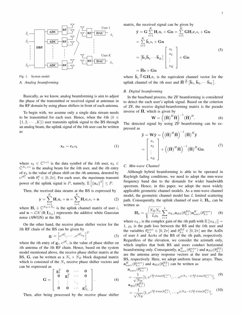
VI. SIMULATIONS
In this section, numerical results are presented to verifythe proposed data-driven analog beam selection method. Wemodel path loss of k-user as ρk = D
−β/2k where Dk is the
distance between the BS and the kth user and β is the pathloss exponent. Here, we set β = 3.76. The number of users ineach cell K is set to 10. For simplicity, the distance betweeneach user and the BS Dk is a variable uniformly distributedwith the interval [10, 15]. Besides, we set Ns = K, NR = 5and Nu = 5. For the mm-wave channel, we set the number ofscattering path L = 4 and the azimuth angles of departure orarrival of user and the BS are uniformly distributed between 0and 2π, signal wavelength λ=5 mm and the antenna spacingdistance λ/2. We assume there are 5 candidates of transmitanalog beams, which can be represented as
F =c1, c2, c3, c4, c5
(46)
where codeword cn can be expressed as
cn =1√Nu
[1, e−j2π1n∗
, e−j2π2n∗, · · · , e−j2π(Nu−1)n∗
]T(47)
with n∗ = n−1|F| . Besides, we assume there are three candidates
of receive analog beams in G, and each codeword is alsostructured by the rule (47).
−5 0 5 10 15 20 256
8
10
12
14
16
18
20
22
SNR (dB)
Ave
rage
upl
ink
sum
−ra
te (
bps/
Hz)
Data−driven method with M=2×10³
Data−driven method with M=4×10³
Sub−optimizationExhaustive search
Fig. 3. Average uplink sum-rate versus SNR
Fig. 3 shows the average uplink sum-rate under differentSNR, where the average sum-rate is obtained over 10000channel realizations. One may note that the sum-rate of data-driven analog beam selection method with M = 4×10³ is veryclose to the sub-optimization method. However, as shown inFig.3, the data-driven method with M = 2× 10³ brings aboutan obvious degression of uplink sum-rate.
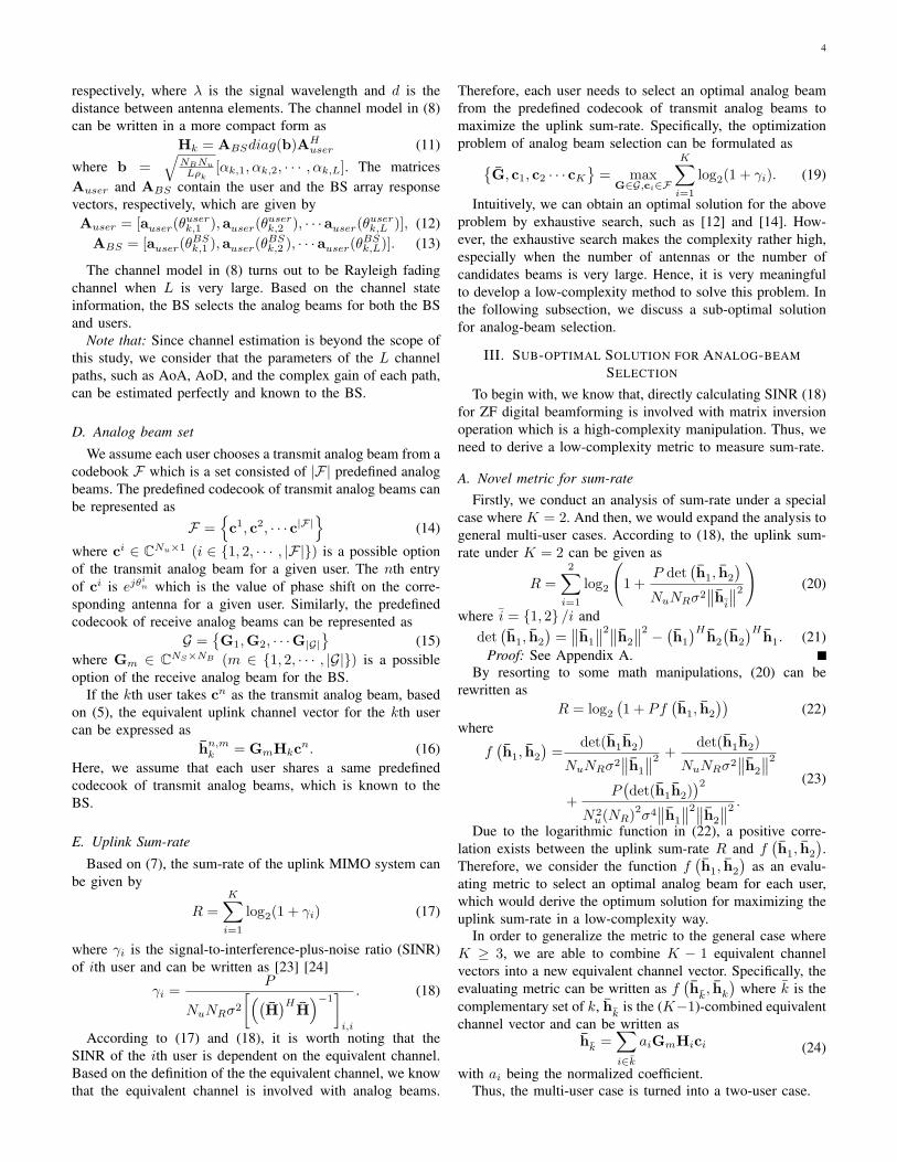
Fig. 4 shows the average uplink sum-rate versus numberof training samples. One may note that the sum-rate of data-driven analog beam selection method tends to close to thesum-rate of sub-optimization method as the number of training
1000 2000 3000 4000 5000 6000 7000 8000 9000 100008.5
9
9.5
10
10.5
11
11.5
12
12.5
13
Number of training samples
Ave
rage
upl
ink
sum
−ra
te (
bps/
Hz)
Data−driven methodSub−optimizationExhaustive search
SNR=5 dB
SNR=0 dB
Fig. 4. Average uplink sum-rate versus the number of training samples
samples increases. For example, when the number of trainingsamples is 1000, the sum-rate of data-driven method is 15%lower of the counterpart of the sub-optimization method,which is unacceptable. Nevertheless, when the number oftraining samples is 10000, the sum-rate of data-driven methodis almost the same with the counterpart of the sub-optimizationmethod. Therefore, Fig. 3 and Fig. 4 reveal that the data-driven method is highly dependent on the number of trainingdata. As long as the the number of training data is largeenough, the data-driven method is able to provide a near-optimal performance.
0 2 4 6 8 10 12 14 16
Average uplink sum-rate (bps/Hz)
0
0.1
0.2
0.3
0.4
0.5
0.6
0.7
0.8
0.9
1
CD
F
Empirical CDF
Exhaustive searchSub-optimization
Data-driven method with M=4 103
Data-driven method with M=2 103
Fig. 5. Effectiveness of data-driven method
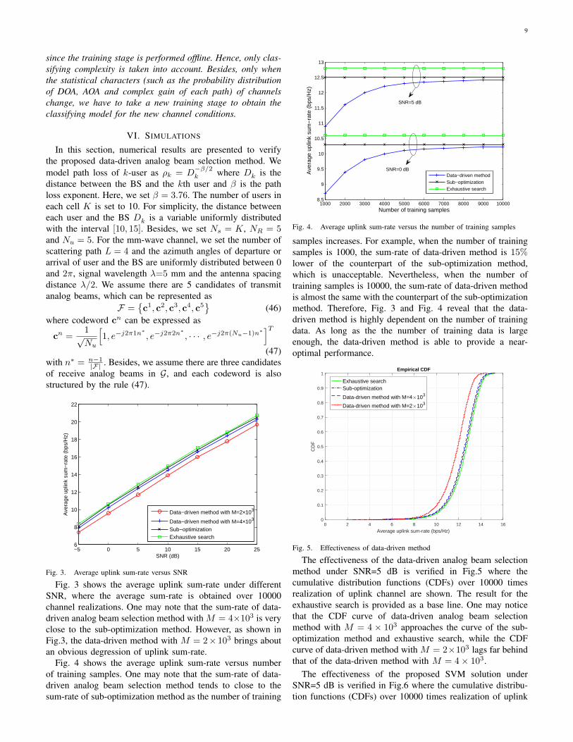
The effectiveness of the data-driven analog beam selectionmethod under SNR=5 dB is verified in Fig.5 where thecumulative distribution functions (CDFs) over 10000 timesrealization of uplink channel are shown. The result for theexhaustive search is provided as a base line. One may noticethat the CDF curve of data-driven analog beam selectionmethod with M = 4 × 10³ approaches the curve of the sub-optimization method and exhaustive search, while the CDFcurve of data-driven method with M = 2×10³ lags far behindthat of the data-driven method with M = 4× 10³.
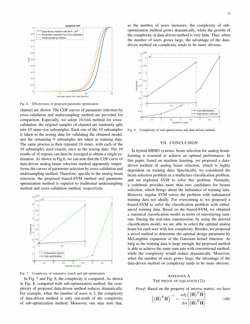
The effectiveness of the proposed SVM solution underSNR=5 dB is verified in Fig.6 where the cumulative distribu-tion functions (CDFs) over 10000 times realization of uplink
10
0 5 10 15
Average uplink sum-rate (bps/Hz)
0
0.1
0.2
0.3
0.4
0.5
0.6
0.7
0.8
0.9
1C
DF
Empirical CDF
Data-driven method with M=4 103
Parameter selection by cross-validationUndersampling method
Fig. 6. Effectiveness of proposed parameter optimization
channel are shown. The CDF curves of parameter selection bycross-validation and undersampling method are provided forcomparison. Especially, we adopt 10-fold method for cross-validation, the original samples of channel are randomly splitinto 10 same-size subsamples. Each one of the 10 subsamplesis taken as the testing data for validating the obtained model,and the remaining 9 subsamples are taken as training data.The same process is then repeated 10 times, with each of the10 subsamples used exactly once as the testing data. The 10results of 10 repeats can then be averaged to obtain a single es-timation. As shown in Fig.6, we can note that the CDF curve ofdata-driven analog beam selection method apparently outper-forms the curves of parameter selection by cross-validation andundersampling method. Therefore, specific to the analog beamselection, the proposed biased-SVM method and parameteroptimization method is superior to traditional undersamplingmethod and cross-validation method, respectively.
2 2.5 3 3.5 4 4.5 5 5.5 6
Number of users
0
1
2
3
4
5
6
7
8
9
Com
plex
ity
1011
2 2.5 30
0.5
1
1.5
2
2.5
3
3.5
4
4.5108
Exhaustive searchSub-optimization
Fig. 7. Complexity of exhaustive search and sub-optimization
In Fig. 7 and Fig. 8, the complexity is compared. As shownin Fig. 8, compared with sub-optimization method, the com-plexity of proposed data-driven method reduces dramatically.For example, when the number of users is 2, the complexityof data-driven method is only one-tenth of the complexityof sub-optimization method. Moreover, one may note that,
as the number of users increases, the complexity of sub-optimization method grows dramatically, while the growth ofthe complexity of data-driven method is very little. Thus, whenthe number of users grows large, the advantage of the data-driven method on complexity tends to be more obvious.
2 2.5 3 3.5 4 4.5 5 5.5 6
Number of users
0
0.5
1
1.5
2
2.5
3
3.5
4
4.5
5
Com
plex
ity
108
2 2.5 30
0.5
1
1.5
2
2.5
3107
Sub-optimizationData-driven method
Fig. 8. Complexity of sub-optimization and data-driven method
VII. CONCLUSION
In hybrid MIMO systems, beam selection for analog beam-forming is essential to achieve an optimal performance. Inthis paper, based on machine learning, we proposed a data-driven method of analog beam selection, which is highlydependent on training data. Specifically, we considered thebeam selection problem as a multiclass-classification problem,and we exploited SVM to solve this problem. Normally,a codebook provides more than two candidates for beamsselection, which brings about the imbalance of training data.However, regular SVM solves the problem with imbalancedtraining data not ideally. For overcoming it, we proposed abiased-SVM to solve the classification problem with imbal-anced training data. Based on the biased-SVM, we obtaineda statistical classification model in terms of maximizing sum-rate. During the real-time transmission, by using the derivedclassification model, we are able to select the optimal analogbeam for each user with low complexity. Besides, we proposeda novel method to determine the optimal design parameter byMcLaughlin expansion of the Gaussian kernel function. Aslong as the training data is large enough, the proposed methodis able to achieve the same sum-rate with conventional method,while the complexity would reduce dramatically. Moreover,when the number of users grows large, the advantage of thedata-driven method on complexity tends to be more obvious.
APPENDIX ATHE PROOF OF EQUATION (21)
Proof: Based on the property of inverse matrix, we have((H)H
H)−1
=adj((
H)H
H)
det∣∣∣(H)HH
∣∣∣ (48)

11
where adj((
H)H
H)
represents the adjugate of matrix(H)H
H.
To begin with, adj((
H)H
H)
can be written as
adj((
H)H
H)=
[ ∥∥h2
∥∥2 −(h1
)Hh2
−(h2
)Hh1
∥∥h1
∥∥2]. (49)
Then, det∣∣∣(H)HH
∣∣∣ can be written as
det∣∣∣(H)HH
∣∣∣ = ∥∥h1
∥∥2∥∥h2
∥∥2 − (h1
)Hh2
(h2
)Hh1. (50)
Substituting (49) and (50) into (48), we arrive at((H)H
H)−1
=1∥∥h1
∥∥2∥∥h2
∥∥2 − (h1
)Hh2
(h2
)Hh1
×
[ ∥∥h2
∥∥2 −(h1
)Hh2
−(h2
)Hh1
∥∥h1
∥∥2].
(51)
According to (18), the SINR of user 1 and 2 can be writtenas
γ1 =P
NuNRσ2
[((H)H
H)−1
]1,1
=P(∥∥h1
∥∥2∥∥h2
∥∥2 − (h1
)Hh2
(h2
)Hh1
)NuNRσ2
∥∥h2
∥∥2 ,
γ2 =P
NuNRσ2
[((H)H
H)−1
]2,2
=P(∥∥h1
∥∥2∥∥h2
∥∥2 − (h1
)Hh2
(h2
)Hh1
)NuNRσ2
∥∥h1
∥∥2 ,
(52)
respectively.The proof is completed by substituting (52) into (7).
APPENDIX BEQUATION (21)
Proof: Firstly, based on the definition of Forbinius norm,we have,||ϕ(ti)− ϕ(tj)||2
= ⟨ϕ(ti), ϕ(ti)⟩+ ⟨ϕ(tj), ϕ(tj)⟩ − 2 ⟨ϕ(ti), ϕ(tj)⟩ .(53)
By resorting to the fact K(ti, tj)= ⟨ϕ(ti), ϕ(tj)⟩, the aboveformula can be further written as||ϕ(ti)− ϕ(tj)||2
= K (ϕ(ti), ϕ(ti)) +K (ϕ(tj), ϕ(tj))− 2K (ϕ(ti), ϕ(tj)) .(54)
Based on Gaussian radial-based kernel function, i.e.,K(ti, tj) = e(−∥ti−tj∥2/(2σ2)), we have
K (ϕ(ti), ϕ(ti)) = K (ϕ(tj), ϕ(tj)) = 1. (55)By substituting the above results into (54), we arrive at
||ϕ(ti)− ϕ(tj)||2 = 2− 2K (ϕ(ti), ϕ(tj)) . (56)Thus, the proof of the result is completed.
REFERENCES
[1] J. G. Andrews, S. Buzzi, W. Choi, S. V. Hanly, A. Lozano, A. C. Soong,and J. C. Zhang, “What will 5G be?” IEEE J. Sel. Areas Commun.,vol. 32, no. 6, pp. 1065–1082, 2014.
[2] Z. Pi and F. Khan, “An introduction to millimeter-wave mobile broad-band systems,” IEEE Commun. Mag., vol. 49, no. 6, 2011.
[3] T. S. Rappaport, S. Sun, R. Mayzus, H. Zhao, Y. Azar, K. Wang, G. N.Wong, J. K. Schulz, M. Samimi, and F. Gutierrez, “Millimeter wavemobile communications for 5G cellular: It will work!” IEEE Access,vol. 1, pp. 335–349, 2013.
[4] W. Roh, J.-Y. Seol, J. Park, B. Lee, J. Lee, Y. Kim, J. Cho, K. Cheun, andF. Aryanfar, “Millimeter-wave beamforming as an enabling technologyfor 5G cellular communications: Theoretical feasibility and prototyperesults,” IEEE Commun. Mag., vol. 52, no. 2, pp. 106–113, 2014.
[5] C. Wang and H.-M. Wang, “Physical layer security in millimeter wavecellular networks,” IEEE Trans. on Wireless Commu., vol. 15, no. 8, pp.5569–5585, 2016.
[6] H.-M. W. Y. Ju and T.-X. Zheng, “Secure transmissions in millimeterwave systems,” IEEE Trans. on Commu., vol. 65, no. 5, pp. 2114–2127,2017.
[7] E. G. Larsson, O. Edfors, F. Tufvesson, and T. L. Marzetta, “MassiveMIMO for next generation wireless systems,” IEEE Commun. Mag.,vol. 52, no. 2, pp. 186–195, 2014.
[8] L. Lu, G. Y. Li, A. L. Swindlehurst, A. Ashikhmin, and R. Zhang, “Anoverview of massive MIMO: Benefits and challenges,” IEEE J. Sel.Topics Signal Process., vol. 8, no. 5, pp. 742–758, 2014.
[9] X. Gao, L. Dai, S. Han, I. Chih-Lin, and R. W. Heath, “Energy-efficienthybrid analog and digital precoding for mmwave mimo systems withlarge antenna arrays,” IEEE J. Sel. Areas Commun., vol. 34, no. 4, pp.998–1009, 2016.
[10] H. Lin, F. Gao, S. Jin, and G. Y. Li, “A new view of multi-user hybridmassive MIMO: Non-orthogonal angle division multiple access,” IEEEJ. Sel. Areas Commun., vol. PP, no. 99, pp. 1–1, 2017.
[11] J. Zhao, F. Gao, W. Jia, S. Zhang, S. Jin, and H. Lin, “Angle domainhybrid precoding and channel tracking for mmwave massive MIMOsystems,” IEEE Trans. on Wireless Commu., vol. PP, no. 99, pp. 1–1,2017.
[12] Y. Niu, Z. Feng, Y. Li, Z. Zhong, and D. Wu, “Low complexity andnear-optimal beam selection for millimeter wave MIMO systems,” inWireless Communications and Mobile Computing Conference, 2017 13thInternational. IEEE, 2017, pp. 634–639.
[13] Y. Gao, M. Khaliel, T. Kaiser et al., “Rotman lens based hybrid analog-digital beamforming in massive MIMO systems: Array architectures,beam selection algorithms and experiments,” IEEE Trans. Veh. Technol.,2017.
[14] Y. Ren, Y. Wang, C. Qi, and Y. Liu, “Multiple-beam selection withlimited feedback for hybrid beamforming in massive MIMO systems,”IEEE Access, 2017.
[15] F. Provost and T. Fawcett, “Data science and its relationship to big dataand data-driven decision making,” Big Data, vol. 1, no. 1, pp. 51–59,2013.
[16] C. P. Chen and C.-Y. Zhang, “Data-intensive applications, challenges,techniques and technologies: A survey on big data,” Information Sci-ences, vol. 275, pp. 314–347, 2014.
[17] S. Bi, R. Zhang, Z. Ding, and S. Cui, “Wireless communications in theera of big data,” IEEE Commun. Mag., vol. 53, no. 10, pp. 190–199,2015.
[18] A. Imran, A. Zoha, and A. Abu-Dayya, “Challenges in 5g: how toempower SON with big data for enabling 5G,” IEEE Network, vol. 28,no. 6, pp. 27–33, 2014.
[19] R. S. Michalski, J. G. Carbonell, and T. M. Mitchell, Machine learning:An artificial intelligence approach. Springer Science & Business Media,2013.
[20] C. Cortes and V. Vapnik, “Support vector machine,” Machine Learning,vol. 20, no. 3, pp. 273–297, 1995.
[21] F. Lotte, M. Congedo, A. Lecuyer, F. Lamarche, and B. Arnaldi,“A review of classification algorithms for eeg-based brain–computerinterfaces,” Journal of Neural Engineering, vol. 4, no. 2, p. R1, 2007.
[22] M. R. Akdeniz, Y. Liu, M. K. Samimi, S. Sun, S. Rangan, T. S.Rappaport, and E. Erkip, “Millimeter wave channel modeling andcellular capacity evaluation,” IEEE J. Sel. Areas Commun., vol. 32, no. 6,pp. 1164–1179, 2014.
[23] M. Matthaiou, C. Zhong, and T. Ratnarajah, “Novel generic bounds onthe sum rate of MIMO ZF receivers,” IEEE Trans. on Signal Processing,vol. 59, no. 9, pp. 4341–4353, 2011.
[24] M. Matthaiou, C. Zhong, M. R. Mckay, and T. Ratnarajah, “Sum rateanalysis of zf receivers in distributed MIMO systems,” IEEE J. Sel.Areas Commun., vol. 31, no. 2, pp. 180–191, 2013.
[25] J. Platt, “Sequential minimal optimization: A fast algorithm for trainingsupport vector machines,” 1998.
[26] S. Arlot, A. Celisse et al., “A survey of cross-validation procedures formodel selection,” Statistics surveys, vol. 4, pp. 40–79, 2010.
12
[27] X.-R. Cao, “The maclaurin series for performance functions of markovchains,” Advances in Applied Probability, vol. 30, no. 3, pp. 676–692,1998.
[28] R. Raz, “On the complexity of matrix product,” In Proceedings of thethirty-fourth annual ACM symposium on Theory of computing, vol. 32,no. 5, 2002.
[29] J. Joung, “Machine learning-based antenna selection in wireless com-munications,” IEEE Comm. Lett., vol. 20, no. 11, pp. 2241–2244, 2016.
Yin Long received the M.S. degree in communica-tion engineering from the Chongqing University ofPosts and Telecommunications, Chongqing, China,in 2013. He is currently pursuing the Ph.D. degreein communication with the National Key Laboratoryof Science and Technology on Communications,University of Electronic Science and Technologyof China, Chengdu, China. He was a Visiting S-tudent with the University of Alberta, Edmonton,Alberta, Canada, from 2016 to 2017. His currentresearch interests include massive MIMO, random
matrix theory and data mining. He has served as a Reviewer for variousinternational journals and conferences, including the IEEE TRANSACTIONSON COMMUNICATIONS and the IEEE TRANSACTIONS ON WIRELESSCOMMUNICATIONS.
Zhi Chen (M’08-SM’16) received the B.S., M.S.,and Ph.D. degrees in electrical engineering from theUniversity of Electronic Science and Technology ofChina (UESTC), Chengdu, China, in 1997, 2000,and 2006, respectively. In 2006, he joined the Na-tional Key Laboratory of Science and Technologyon Communications, UESTC, where he has been aProfessor since 2013. He was a Visiting Scholar withthe University of California at Riverside, Riverside,CA, USA, from 2010 to 2011. His current researchinterests include 5G mobile communications, tactile
Internet, and terahertz communication. He has served as a Reviewer for var-ious international journals and conferences, including the IEEE TRANSAC-TIONS ON VEHICULAR TECHNOLOGY and the IEEE TRANSACTIONSON SIGNAL PROCESSING.
Jun Fang (M’08) received the B.S. and M.S. de-grees from Xidian University, Xian, China, in 1998and 2001, respectively, and the Ph.D. degree fromthe National University of Singapore, Singapore, in2006, all in electrical engineering. During 2006, hewas a Post-Doctoral Research Associate with theDepartment of Electrical and Computer Engineering,Duke University. From 2007 to 2010, he was aResearch Associate with the Department of Electri-cal and Computer Engineering, Stevens Institute ofTechnology. Since 2011, he has been with the Uni-
versity of Electronic of Science and Technology of China. His current researchinterests include sparse theory and compressed sensing, statistical learning,millimeter Wave, and massive MIMO communications. Dr. Fang receivedthe IEEE Jack Neubauer Memorial Award in 2013 for the best systems paperpublished in the IEEE TRANSACTIONS ON VEHICULAR TECHNOLOGY.He is an Associate Technical Editor for the IEEE Communications Magazine,and an Associate Editor of the IEEE SIGNAL PROCESSING LETTERS.
Chintha Tellambura (F’11) received the B.Sc. de-gree (with first-class honor) from the University ofMoratuwa, Sri Lanka, the MSc degree in Electronicsfrom Kings College, University of London, UnitedKingdom, and the PhD degree in Electrical Engi-neering from the University of Victoria, Canada.
He was with Monash University, Australia, from1997 to 2002. Presently, he is a Professor with theDepartment of Electrical and Computer Engineering,University of Alberta. His current research interestsinclude the design, modelling and analysis of cog-
nitive radio, heterogeneous cellular networks and 5G wireless networks.Prof. Tellambura served as an editor for both IEEE Transactions on
Communications (1999-2011) and IEEE Transactions on Wireless Communi-cations (2001-2007) and for the latter he was the Area Editor for WirelessCommunications Systems and Theory during 2007-2012. He has receivedbest paper awards in the Communication Theory Symposium in 2012 IEEEInternational Conference on Communications (ICC) in Canada and 2017 ICCin France. He is the winner of the prestigious McCalla Professorship and theKillam Annual Professorship from the University of Alberta. In 2011, he waselected as an IEEE Fellow for his contributions to physical layer wirelesscommunication theory. In 2017, he was elected as a Fellow of CanadianAcademy of Engineering. Prof. Tellambura has authored or coauthored over500 journal and conference papers with total citations more than 14,000 andan h-index of 64 (Google Scholar).