data-driven nonlinear control designs for constrained systems
TRANSCRIPT

University of Central Florida University of Central Florida
STARS STARS
Electronic Theses and Dissertations, 2020-
2020
Data-Driven Nonlinear Control Designs for Constrained Systems Data-Driven Nonlinear Control Designs for Constrained Systems
Roland Harvey University of Central Florida
Part of the Computer Engineering Commons
Find similar works at: https://stars.library.ucf.edu/etd2020
University of Central Florida Libraries http://library.ucf.edu
This Doctoral Dissertation (Open Access) is brought to you for free and open access by STARS. It has been accepted
for inclusion in Electronic Theses and Dissertations, 2020- by an authorized administrator of STARS. For more
information, please contact [email protected].
STARS Citation STARS Citation Harvey, Roland, "Data-Driven Nonlinear Control Designs for Constrained Systems" (2020). Electronic Theses and Dissertations, 2020-. 53. https://stars.library.ucf.edu/etd2020/53

DATA-DRIVEN NONLINEAR CONTROL DESIGNS FOR CONSTRAINED SYSTEMS
by
ROLAND HARVEYM.S. University of Central Florida, 2016
B.S. Tulane University, 2014
A dissertation submitted in partial fulfilment of the requirementsfor the degree of Doctor of Philosophy
in the Department of Electrical and Computer Engineeringin the College of Engineering and Computer Science
at the University of Central FloridaOrlando, Florida
Spring Term2020
Major Professor: Zhihua Qu

c© 2020 Roland Harvey
ii

ABSTRACT
Systems with nonlinear dynamics are theoretically constrained to the realm of nonlinear analysis
and design, while explicit constraints are expressed as equalities or inequalities of state, input, and
output vectors of differential equations. Few control designs exist for systems with such explicit
constraints, and no generalized solution has been provided. This dissertation presents general
techniques to design stabilizing controls for a specific class of nonlinear systems with constraints
on input and output, and verifies that such designs are straightforward to implement in selected
applications. Additionally, a closed-form technique for an open-loop problem with unsolvable
dynamic equations is developed. Typical optimal control methods cannot be readily applied to
nonlinear systems without heavy modification. However, by embedding a novel control framework
based on barrier functions and feedback linearization, well-established optimal control techniques
become applicable when constraints are imposed by the design in real-time. Applications in power
systems and aircraft control often have safety, performance, and hardware restrictions that are
combinations of input and output constraints, while cryogenic memory applications have design
restrictions and unknown analytic solutions. Most applications fall into a broad class of systems
known as passivity-short, in which certain properties are utilized to form a structural framework for
system interconnection with existing general stabilizing control techniques. Previous theoretical
contributions are extended to include constraints, which can be readily applied to the development
of scalable system networks in practical systems, even in the presence of unknown dynamics. In
cases such as these, model identification techniques are used to obtain estimated system models
which are guaranteed to be at least passivity-short. With numerous analytic tools accessible, a
data-driven nonlinear control design framework is developed using model identification resulting
in passivity-short systems which handles input and output saturations. Simulations are presented
that prove to effectively control and stabilize example practical systems.
iii

TABLE OF CONTENTS
LIST OF FIGURES . . . . . . . . . . . . . . . . . . . . . . . . . . . . . . . . . . . . . . vii
LIST OF TABLES . . . . . . . . . . . . . . . . . . . . . . . . . . . . . . . . . . . . . . . x
CHAPTER 1: BACKGROUND . . . . . . . . . . . . . . . . . . . . . . . . . . . . . . . 1
Stability Concepts . . . . . . . . . . . . . . . . . . . . . . . . . . . . . . . . . . . . . . 2
Nonlinear Systems . . . . . . . . . . . . . . . . . . . . . . . . . . . . . . . . . . . . . 3
Dissipativity . . . . . . . . . . . . . . . . . . . . . . . . . . . . . . . . . . . . . . . . . 6
Optimal Control with Exogenous Input . . . . . . . . . . . . . . . . . . . . . . . . . . . 11
Dynamic Inversion . . . . . . . . . . . . . . . . . . . . . . . . . . . . . . . . . . . . . 15
Jacobian Equivalence . . . . . . . . . . . . . . . . . . . . . . . . . . . . . . . . . . . . 18
Hammerstein-Wiener Model Identification . . . . . . . . . . . . . . . . . . . . . . . . . 19
CHAPTER 2: OPTIMIZED INPUT/OUTPUT-CONSTRAINED CONTROL DESIGN . . 22
Barrier Formulation . . . . . . . . . . . . . . . . . . . . . . . . . . . . . . . . . . . . . 24
Barrier Function Design . . . . . . . . . . . . . . . . . . . . . . . . . . . . . . . . . . . 29
CHAPTER 3: MICROGRID CONTROL WITH HIGH-PENETRATION OF PHOTOVOLTAICS
iv

39
Constrained Control in a Microgrid . . . . . . . . . . . . . . . . . . . . . . . . . . . . . 41
PV, Duck Curve, and Saturations . . . . . . . . . . . . . . . . . . . . . . . . . . . . . . 42
Simulation and Discussion . . . . . . . . . . . . . . . . . . . . . . . . . . . . . . . . . 49
CHAPTER 4: NONLINEAR AUTOPILOT DESIGN . . . . . . . . . . . . . . . . . . . . 57
Problem Formulation . . . . . . . . . . . . . . . . . . . . . . . . . . . . . . . . . . . . 58
Nonlinear Control for Autopilot . . . . . . . . . . . . . . . . . . . . . . . . . . . . . . 60
Software Framework . . . . . . . . . . . . . . . . . . . . . . . . . . . . . . . . . . . . 61
HW Modeling . . . . . . . . . . . . . . . . . . . . . . . . . . . . . . . . . . . . . . . . 65
Real-Time Data-Driven Modeling and Control . . . . . . . . . . . . . . . . . . . . . . . 70
CHAPTER 5: CRYOGENIC MEMORY STATE TRANSITIONS . . . . . . . . . . . . . 74
Equilibrium Definitions . . . . . . . . . . . . . . . . . . . . . . . . . . . . . . . . . . . 76
Memory Control Design . . . . . . . . . . . . . . . . . . . . . . . . . . . . . . . . . . 78
Memory Cell Control Validation . . . . . . . . . . . . . . . . . . . . . . . . . . . . . . 90
CHAPTER 6: CONCLUSION . . . . . . . . . . . . . . . . . . . . . . . . . . . . . . . . 95
APPENDIX
v

LIST OF PUBLICATIONS . . . . . . . . . . . . . . . . . . . . . . . . . . . 96
LIST OF REFERENCES . . . . . . . . . . . . . . . . . . . . . . . . . . . . . . . . . . . 98
vi

LIST OF FIGURES
1.1 Passivity-Short System with Output Saturation Block Diagram . . . . . . . . 10
1.2 Passivity-Short System with Input Saturation Block Diagram . . . . . . . . . 11
1.3 Feedback Linearization General Procedure Diagram . . . . . . . . . . . . . . 15
1.4 Hammerstein-Wiener Model Block Diagram . . . . . . . . . . . . . . . . . . 21
2.1 Barrier Function in Optimal Control Block Diagram . . . . . . . . . . . . . . 33
2.2 Control and State Trajectories of Input Rate Saturated System . . . . . . . . . 36
3.1 Sample Net Load Profile with Intermittent Solar Generation . . . . . . . . . . 43
3.2 Trajectory of ug and its Limiting Values . . . . . . . . . . . . . . . . . . . . 46
3.3 Difference in Forecast vs. Actual Net Load due to Solar Generation . . . . . 47
3.4 Integration of Difference in Forecast vs. Actual Net Load . . . . . . . . . . . 48
3.5 Frequency and Traditional Generation at 100% solar penetration, us = 0.1 . . 50
3.6 Frequency and Traditional Generation at 100% solar penetration, us = 0.22 . 50
3.7 Stressing BESS and DR Behavior due to Low Ramping Rate Limit, us = 0.1,
E = 0.3 . . . . . . . . . . . . . . . . . . . . . . . . . . . . . . . . . . . . . 52
3.8 Frequency and Traditional Generation, us = 0.1, with BESS and DR, E = 0.3 52
vii

3.9 Frequency and Traditional Generation, us = 0.22, with BESS, E = 0.3,
without DR . . . . . . . . . . . . . . . . . . . . . . . . . . . . . . . . . . . 53
3.10 BESS Behavior without DR, E = 0.3 . . . . . . . . . . . . . . . . . . . . . 53
3.11 Frequency and Traditional Generation, us = 0.22, with BESS, E = 0.07,
and DR . . . . . . . . . . . . . . . . . . . . . . . . . . . . . . . . . . . . . 54
3.12 Optimal BESS and DR Behavior, E = 0.07 . . . . . . . . . . . . . . . . . . 54
4.1 Coordinate Frame and Angle Convention for Aerial Vehicles with Canards . . 59
4.2 6 Degree-of-Freedom Aerial Vehicle Simulation Block Diagram . . . . . . . 62
4.3 Pitch Channel Acceleration Command Response . . . . . . . . . . . . . . . . 63
4.4 Yaw Channel Acceleration Command Response . . . . . . . . . . . . . . . . 63
4.5 Simultaneous Pitch and Yaw Acceleration Command Responses . . . . . . . 64
4.6 Acceleration Response with Constraints Imposed on α and β . . . . . . . . . 65
4.7 HW Model Comparison with Measured Data in Unconstrained Single Channel 66
4.8 HW Model Comparison in Pitch Channel with Constraints . . . . . . . . . . 67
4.9 HW Model Comparison in Yaw Channel with Constraints . . . . . . . . . . . 67
4.10 Indirect Adaptive Approach to Data-Driven Modeling and Control . . . . . . 72
5.1 Isoclines and Equilibria of Autonomous Nonlinear Oscillator . . . . . . . . . 77
viii

5.2 Single Uncoupled Oscillator Equilibrium Definitions . . . . . . . . . . . . . 79
5.3 Coupled Oscillator Sample Trajectories with Boundaries . . . . . . . . . . . 80
5.4 Elliptic Function Values for Λ = π/2 . . . . . . . . . . . . . . . . . . . . . . 82
5.5 A Typical Gaussian Pulse with Defined Amplitude . . . . . . . . . . . . . . 85
5.6 A Saturated Gaussian Pulse . . . . . . . . . . . . . . . . . . . . . . . . . . . 87
5.7 Intersection of Pulse Controlled Oscillator with Linear Trajectory Objective . 90
5.8 Three-Junction Memory Transition 0, 0, 0 → 2, 1, 0, Dual Pulse . . . . . 91
5.9 Three-Junction Memory Transition 0, 0, 0 → 2, 1, 0, Single Pulse . . . . 92
5.10 Three-Junction Memory Transition 0, 0, 0 → 3, 2, 0, Single Pulse . . . . 93
ix

LIST OF TABLES
5.1 Transition Pulse Gains . . . . . . . . . . . . . . . . . . . . . . . . . . . . . 93
x

NOMENCLATURE
Symbol/Abbreviation Description
BESS Battery Energy Storage System
DR Demand Response
HW Hammerstein-Wiener (model identification)
ε Impact Coefficient for Input of Passivity-short Systems
ρ Impact Coefficient for Output of Passivity-short Systems
s Laplace Operator, Derivative
L−1 Inverse Laplace Transform
I Identity Matrix
Lf Lie Derivative w.r.t. function f
r, r Exogenous Input and Estimation
µi Relative Degree for System i
V, Vi Energy Storage Function, Storage Function for System i
5t Gradient Operator w.r.t. Variable t
αi Expanded Polynomial Inequality for Barrier i
E Upper Bound on Battery Energy
us Upper Bound on Traditional Generation Ramping Rate
ω0 Nominal Frequency for Power Systems
α Angle of Attack
β Sideslip Angle
ωB = [p q r]T Body Frame Angular Rate Vector
VB = [u v w]T Body Frame Velocity Vector
MB Body Frame Moment
xi

JB Body Frame Inertia Matrix
m Vehicle Mass
FB Body Frame Applied Force
δ Canard Angle Deflection
γi Damping Coefficient for System i
µi Coupling Coefficient for Oscillators
ki Pulse Gain for Oscillator i
ni Desired Equilibrium Triplet
δ(t) Unit Impulse, Delta Function
Λ Elliptic Integral Upper Limit Angle
f id Damping Force for Oscillator i
Ei Energy in Oscillator i
W Work Done by Damping
xii

CHAPTER 1: BACKGROUND
Recently, there have been few nonlinear control designs for constrained systems that can be used
for different applications. As shown in [1] and [2], specific designs to deal with specific applica-
tions have been developed, but are lacking in generalization to other systems. In most practical
cases, the properties of an entire class of systems may be utilized as a design tool. Scalability is
an important property that is lacking for existing tools developed for linear systems. For instance,
analysis in the Laplace domain becomes daunting to use on a large scale network of systems,
however, the passivity-short framework may be used instead for such networks, which also ap-
plies to nonlinear systems. Although optimal control was developed decades ago, there are still
developments that can be made to improve applicability where real time control is necessary. Com-
binations of data-driven control designs and optimization are required to ensure safety and optimal
performance. If model dynamics are unknown, then system identification techniques are required
to design an effective controller.
In this chapter, some existing techniques, definitions, and properties are presented that will be uti-
lized in subsequent chapters. As such, these tools are useful in regards to control and system design
which are applied to various problems in unique ways. Additionally, this foundation provides a
baseline on which further developments will be presented. Mathematical concepts that serve as the
starting point from which powerful tools for systems and controls are presented, starting with the
concept of system stability.
1

Stability Concepts
The underlying concept of system stability is based on whether output can be bounded given a
bounded input. Specifically, if there exists a bound on input, then must exist a bound on output
to achieve stability. This concept is referred to as bounded-input bounded-output (BIBO) stability.
For nonlinear systems, this idea is the first and foremost definition that is addressed. Without
defining stability, we are unable to quantify performance of systems or controls, or even design
adequate controls for systems. Linear system stability has been well-established and thoroughly
investigated, so only brief definitions will be provided.
Consider the general linear system:
x = Ax+Bu
y = Cx+Du,
(1.1)
where x ∈ <n, u ∈ <m, y ∈ <p, and A,B,C,D are matrices of appropriate dimension.
Lemma 1 If u = 0, system (1.1) is said to be stable if one of the following equivalent items is true:
• Real parts of eigenvalues of A are nonpositive
• A ≤ 0 (matrix A is negative semi-definite)
• Roots of L−1[sI − A]−1 are in the right half-plane
System (1.1) is said to be asymptotically stable if eigenvalues of A have a strictly negative real
part, or A < 0, or roots of L−1[sI − A]−1 have strictly positive real parts.
It should be noted that stability is tested while either the system behaves autonomously, or the
2

control u is designed to close the loop. If a system is not stable with u = 0, a control can be
designed to stabilize the system if the system has some degree of controllability and observability.
Nonlinear Systems
Concepts of stability for nonlinear systems require a different approach than linear systems, since
all stability definitions for linear systems depend on linearity of dynamics. However, definitions
of stability for nonlinear systems can be generalized to linear systems as well, although it may be
easier to use linear system stability concepts when dealing with linear systems. Nevertheless, a
general nonlinear affine system is presented as follows:
x = f(x) + g(x)u
y = h(x),
(1.2)
where x ∈ <n, u ∈ <m, y ∈ <p, and f(x), g(x), and h(x) are nonlinear in general and of
appropriate dimension. Conveniently presented in [3], a common tool which is used to show
stability for nonlinear systems is known as the Lyapunov direct method. This technique requires
choosing an energy-like storage function V (x) which is generally positive definite, and must be
a function of all internal state variables. Additionally, V (x) = 0 must only occur when x = 0.
By default, Lyapunov’s method is valid for equilibrium points at the origin, however, they can be
easily shifted by state augmentation. The following definition restates Lyapunov’s direct method
for nonlinear system stability:
Definition 1 System (1.2) is said to be Lyapunov stable (at least marginally stable) if, for storage
function V (x) > 0, V (x) ≤ 0 for all x 6= 0. Additionally, system (1.2) is said to be asymptotically
stable if V (x) < 0 for all x 6= 0.
3

Lyapunov method analysis for energy storage functions (also called Lyapunov candidates) is based
on sufficiency. Unfortunately, if one cannot show that for V (x) > 0, V (x) ≤ 0, then the system’s
stability is inconclusive. Much of the process to prove stability in this manner resides in the
selection of the correct Lyapunov candidate, in which quadratic functions are typically chosen first
due to simplicity. The concept is illustrated in the following example:
Example 1 Consider the system:
x+ x3 + x = 0
Choosing the storage function as V (x) = 12x2 + 1
2x2 yields
V (x) = −x4,
which satisfies conditions of Definition 1 for stability.
A significant reason to choose Lyapunov candidates as quadratic is due to the energy-like nature of
the behavior. In example 1, the storage function is chosen to be exactly the summation of kinetic
and potential energies of the system. This choice provides insight to the physical behavior, and
since the analysis resulted in V (x) < 0, it is implied that energy is completely conserved and
never lost during transience. It is not always possible to show stability with quadratic candidates,
in which cases a new candidate function may be chosen.
Another type of stability that was first shown in [4] connects state equations with input-output
relationships is known as input-to-state stability (ISS). The concept is defined briefly below.
Definition 2 System (1.2) is said to be input-to-state stable if there exists a continuously increasing
function ζ+ with ζ+(0) = 0, and a function ζ−(x0, t) for all t ≥ 0 which is continuously decreasing
4

to zero for all x0 > 0, such that the following inequality holds:
|x(t)| ≤ ζ−(|x0|, t) + ζ+(‖u‖),
where ζ+ is called the gain.
When ISS has an input equal to zero, it can be seen that system (1.2) becomes globally asymp-
totically stable. Then, the inequality in Definition 2 reduces to |x(t)| ≤ ζ−(|x0|, t). In fact, ISS
implies that a system is globally asymptotically stable with zero input, and BIBO stable if the
output of the system is equal to the state.
A similar stability concept that involves input and output bounds is known as L2 stability based on
the L2 norm, which is equivalent to the Euclidean norm, and is briefly defined as follows [3]:
Definition 3 System (1.2) is said to be L2 stable if for storage function V (x) ≥ 0, the following
holds:
V (x) =∂V
∂xf(x, u) ≤ a(γ2‖u‖2 − ‖y‖2), a, γ > 0.
Then for each x(0) ∈ <n, system (1.2) is finite-gain L2 stable with an L2 gain less than or equal
to γ as
‖y‖L2 ≤ γ‖u‖L2 +
√V (x(0))
a.
In addition to concrete definitions of stability at equilibrium points, the concept of modes exists
to classify behavior around an equilibrium point. Modes are oscillations around an equilibrium
point with a definitive damping and period of oscillation. In rigid-body dynamics (especially aerial
applications), it is usually a design requirement to ensure that all modes are nominally stable.
The following section discusses useful concepts that stem from Lyapunov’s stability definitions
5

and utilize the energy-like nature of the analysis.
Dissipativity
Credited with the introduction of the classification of energy-based analysis of systems, the author
of [5] provides the baseline category on which the remaining concepts are built upon.
Recent research directions require designs of cooperative systems involving distributed controls
with local communication rather than global. The decentralized network framework is becoming
more popular in practice due to safety and security. One such framework is based on passivity,
as shown in [6] and [7]. Specific system structures have been classified as passive in theoretical
environments as in [8], Although passive systems reside in a restrictive subclass of dissipative
systems, very few systems in practice are passive. Graph theoretical methods in [9] have been
developed for communication topology-based design frameworks, which has become a relatively
standard network representation in recent years.
As the name implies, dissipative systems, in general lose energy over time. One exception are
systems which maintain the same amount of energy that is injected. On the other hand, while
inspecting system behavior with a long time horizon, practical systems always lose energy, since
there is physical work being done by the system with respect to the environment, or vice versa.
So-called passive systems encompass systems that never gain energy with respect to the input,
while passivity-short systems may generate some energy during transience. Of course, passivity-
short systems cannot generate more energy than they started with, however, there can be energy
produced based on the input. From this observation, definitions of passive and passivity-short
depend on the relationship between input and output. Although in the scope of this dissertation,
the continuous-time domain is of interest, the discrete-time version of passivity-short theory is
6

discussed in [10] and [11].
Further definitions rely on utilizing the energy storage function and its characteristics from Defini-
tion 1.
Definition 4 System (1.2) is dissipative if, for storage function V (x):
V (x) ≤ −`(x) + uTy + εϕ(u) + ρφ(y),
where `(·), ϕ(·), and φ(·) are positive semi-definite functions and ε and ρ are constant parameters
arising from system dynamics. If storage function V (x) is quadratic, the definition becomes:
V (x) ≤ −a‖x‖2 + uTy + ε‖u‖2 + ρ‖y‖2, (1.3)
where a > 0. The passivity-short system class is a broader class of structure-constrained systems
than passive systems. The structural constraint is that all passivity-short systems must be square,
meaning their input and output dimensions must be equal. The importance in this class of systems
lies in the ability to form a stable plug-and-play network of systems due to underlying proper-
ties. Most practical systems are in fact passivity-short, and can be determined as such through an
energy-based analysis. Recent work which considers general control designs with passivity-short
systems includes [12] and [13], which deal with cooperative design frameworks.
Specific classes which are subcategories of dissipative systems are listed in the following definition,
and depend on the parameters of ε and ρ in (1.3).
Definition 5 System (1.2) with storage function differential (1.3) is said to be:
• passive if ε = ρ = 0;
7

• input passivity-short if ε > 0, ρ = 0;
• output passivity-short if ε = 0, ρ > 0.
More subclasses of dissipative systems are outlined in [3], however, analysis and designs are well-
established for those systems although the subclasses are more restricted than the ones in Definition
5. The realm of passivity-short systems allows relative degrees greater than one, which passivity
does not. Additionally, passivity-short designs for nonminimum phase systems have been devel-
oped in [14], whereas only minimum phase systems can be considered passive. In minimum phase
systems, causality and stability are required for the original system as well as the inverse system.
Equivalently, the linear representation of the system must have all poles and zeros inside the unit
circle. Equivalence in passivity and minimum phase characteristics is investigated in [15], [16],
and [17].
Network stabilizing interconnection of passivity-short systems allows more options than passive
systems, including positive feedback, negative feedback, and a combination of both, as shown in
[12]. Obviously, not all connection schemes are guaranteed to maintain network stability in passive
systems, however, by utilizing this scalable framework, overall networks become plug-and-play
provided that all systems are at least passivity-short.
The following example illustrates the utility of the passivity-short design tool for network stability.
Example 2 Consider the following two systems:
x11 = x12
x12 = −x11 − 3x12 + u1
y1 = x11
x21 = x22
x22 = −2x22 + u2
y2 = x21
8

The storage function candidates for each system are as follows:
V1 =1
2(4x211 + x212) + x12x22, V2 =
1
2(2x221 + x222) + x21x22,
such that:
V1 = −3
2x212 + u1y1 − y21 +
1
2u21 ≤ u1y1 +
1
2u21
V2 = −1
2x222 + u2y2 +
1
2u22 ≤ u2y2 +
1
2u22
When interconnected, we design a positive feedback connection with individual negative feedback
control inputs as u1 = −k1y1 + y2, and u2 = −k2y2 + y1 such that
V1 + V2 = −k1y21 − k2y22 +1
2[k21y
21 − 2k1y1y2 + y22]
= (k212− k1)y21 + (
1
2− k2)y22 − k1y1y2
≤ k21 − k12
y21 + (1 + k1
2− k2)y22
which results in a stable overall system when k1 < 1, and k2 > (1 + k1)/2.
Since Lyapunov stability is based on sufficiency, it is possible that the choices of k1 and k2 are
conservative, however, this also means that stability cannot be guaranteed if the gains violate their
constraints.
Another connection scheme that is relevant in the context of constrained systems and control is
that of a passivity-short and L2 stable system (denoted as PS L2 in Figures 1.1 and 1.2) in series
with a saturation function. Both saturations on output and input are considered, and the analysis is
done independently for each. Specifically, the following lemma is presented:
9

Lemma 2 Consider a system that is passivity-short and L2 stable. Equivalently, from definition 2
in [13], for storage function V > 0,
V ≤ uTy +ε
2‖u‖2 − ρ
2‖y‖2,
where ε, ρ ≥ 0. Then, the system with input and output saturation is also passivity-short and L2
stable as:
V ≤ uTy +ε′
2‖u‖2 − ρ′
2‖y‖2,
where ε′ = 7+2ε2
, and ρ′ = ρ− 2.
Proof: For the configuration shown in Figure 1.1 with saturation on the output and from Definition
5, there exists a storage function V ≥ 0 such that
V ≤ uTv +ε
2‖u‖2 − ρ
2‖v‖2,
with ε, ρ > 0.
Figure 1.1: Passivity-Short System with Output Saturation Block Diagram
Then, it can be concluded that
V = uTy + uT (v − y) +ε
2‖u‖2 − ρ
2‖v‖2
≤ uTy +5 + 2ε
4‖u‖2 − ρ− 1
2‖v‖2,
10
which is passivity-short from u to y with ρ ≥ 1 when the inequality SAT[v]2 ≤ v2 holds. This
can be guaranteed to hold when the saturation function is centered at zero, or can be shifted to be
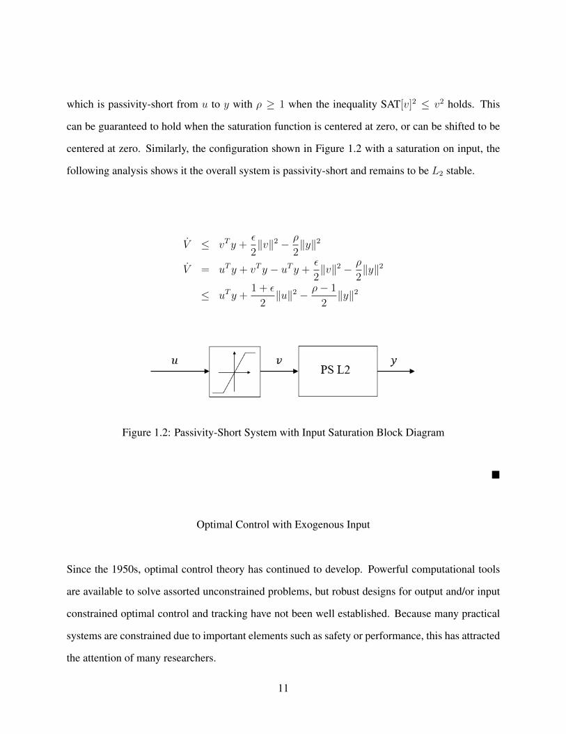
centered at zero. Similarly, the configuration shown in Figure 1.2 with a saturation on input, the
following analysis shows it the overall system is passivity-short and remains to be L2 stable.
V ≤ vTy +ε
2‖v‖2 − ρ
2‖y‖2
V = uTy + vTy − uTy +ε
2‖v‖2 − ρ
2‖y‖2
≤ uTy +1 + ε
2‖u‖2 − ρ− 1
2‖y‖2
Figure 1.2: Passivity-Short System with Input Saturation Block Diagram
Optimal Control with Exogenous Input
Since the 1950s, optimal control theory has continued to develop. Powerful computational tools
are available to solve assorted unconstrained problems, but robust designs for output and/or input
constrained optimal control and tracking have not been well established. Because many practical
systems are constrained due to important elements such as safety or performance, this has attracted
the attention of many researchers.
11

Based on the foundation in Definition 1, a general framework for designing control inputs that
optimally approach equilibrium points was developed most completely in [18], although the math-
ematical theory of calculus of variations was developed much earlier. The strive for advancing
technology that occurred during and after World War II led to important developments involving
previously known mathematics, without a chance for application until that time period. Optimal
control theory, which is still used extensively today, is a Lyapunov-based theory that provides
generally closed form solutions for linear systems, however is somewhat lacking in the realm of
nonlinear systems.
Consider a special case of system (1.2) as follows:
x = F (x) + Ax+Bu+Gr,
y = h(x),
(1.4)
where F (x) is generally nonlinear, A,B,G are constant matrices of appropriate dimension, and
r is an exogenous input. In what follows, an optimal tracking control is derived for system (1.4)
using standard techniques outlined in [19]. Consider the Hamiltonian with costate vector λ(t) as:
H =1
2yTQy +
1
2uTRu+ λT (F (x) + Ax+Bu+Gr), (1.5)
where y = y−yd, yd is the desired output vector, andQ ≥ 0, andR > 0 are constant square penalty
matrices. Then, the corresponding optimization problem is to minimize the following performance
index:
J =1
2yTf Sf yf +
∫ tf
t0
[H− λT x]dt, (1.6)
where Sf ≥ 0 and yf = y(tf ). It follows from calculus of variation [18], [19] that the first-order
12

variation of the performance index is given by
δJ = (Sf yf − λTf )δx
+
∫ tf
t0
[(∂H∂x
+ λ)T δx+ (∂H∂u
)T δu
+(∂H∂λ− x)T δλ
]dt, (1.7)
with λf = Sf∂y∂x|y=yf . By setting δJ in (1.7) equal to zero, the following necessary conditions are
obtained:
x = F (x) + Ax+Bu+Gr, x(t0) = x0
λ = −
(∂y(x)
∂x
T
Q[y(x)− yd]
+[∂F (x)
∂x+ A]Tλ
)u = −R−1BTλ.
Parameterizing the above expression, we know that
λ = k(x, t)− v(r, t),
is a valid choice [19]. Embedding k(x, t) and v(r, t) into the previous equations yields the follow-
13
ing:
∂k(x, t)
∂t=−∂k(x, t)
∂x
T
[F (x) + Ax−BR−1BTk(x, t)]
−∂y(x)
∂x
T
Qy(x)− [∂F (x)
∂x+ A]Tk(x, t), (1.8)
dv(r, t)
dt=
[A−BR−1BT ∂k(x, t)
∂x+∂F (x)
∂x
]Tv(r, t)
−∂k(x, t)
∂xGr +
∂y(x)
∂x
T
Qyd; (1.9)
with terminal conditions k(xf , tf ) = Sfyf , v(r, tf ) = Sfyd.
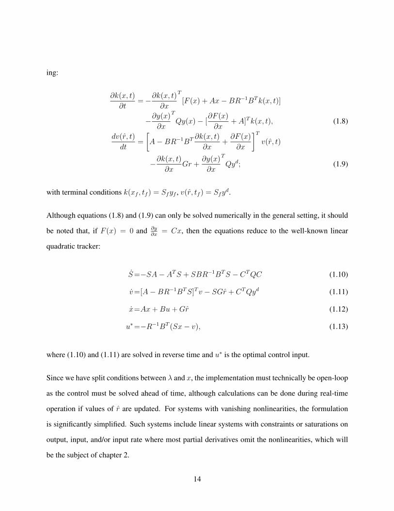
Although equations (1.8) and (1.9) can only be solved numerically in the general setting, it should
be noted that, if F (x) = 0 and ∂y∂x
= Cx, then the equations reduce to the well-known linear
quadratic tracker:
S=−SA− ATS + SBR−1BTS − CTQC (1.10)
v=[A−BR−1BTS]Tv − SGr + CTQyd (1.11)
x=Ax+Bu+Gr (1.12)
u∗=−R−1BT (Sx− v), (1.13)
where (1.10) and (1.11) are solved in reverse time and u∗ is the optimal control input.
Since we have split conditions between λ and x, the implementation must technically be open-loop
as the control must be solved ahead of time, although calculations can be done during real-time
operation if values of r are updated. For systems with vanishing nonlinearities, the formulation
is significantly simplified. Such systems include linear systems with constraints or saturations on
output, input, and/or input rate where most partial derivatives omit the nonlinearities, which will
be the subject of chapter 2.
14

Dynamic Inversion
An important and straightforward approach to design controls for nonlinear systems is known as
dynamic inversion, which is a type of feedback linearization. As the name implies, the dynamics
of the given nonlinear system are linearized in the feedback loop, then stabilized, then returned
to its nonlinear form. This general process is outlined in Figure 1.3. There are a few types of
feedback linearization including state feedback, and additional steps which involve state transfor-
mation, however, these other types will not be considered. Instead, as the input-output feedback
linearization technique in the current context.
Figure 1.3: Feedback Linearization General Procedure Diagram
In a general form, the Lie derivative may be used to describe the first step of the dynamic inversion
process, which is defined as follows:
15

Definition 6 Let Lfh(x) be defined as the Lie derivative of h(x) along f(x) as
Lfh(x) =∂h(x)
∂xf(x).
Additionally, let L(n)f be the recursive Lie derivative as
L(µ)f h(x) =
∂
∂x[L(µ−1)
f h(x)]f(x), (1.14)
which can continue from µ−2 down to µ = 1 recursively, and where µ is called the relative degree.
For a square system, the dimensions of input and output must match, i.e. p = m in system (1.2).
Provided that system (1.2) is square, minimum phase with stable zero dynamics, and that the
derivatives of h(x) remain continuous, the general process of input-output feedback linearization
is presented below using Definition 6:
1. Calculate y(µ) = L(µ)f h(x) + LgL(µ−1)
f h(x)u, where µ is the relative degree
2. Define tracking error e(y(t)), and error differential equation∏µ−1
j=0 (s−aj)e(y(t)) = 0, where
aj > 0 are chosen such that all real parts of s are negative.
3. Solve for the control input as:
u = [LgL(µ−1)f h(x)]−1(−L(µ)
f h(x) +
µ−1∏j=0
(s− aj)e(y(t))). (1.15)
Of course, in order to reach (1.15), both LgL(1)...(µ−2)f h(x) = 0 and LgL(µ−1)
f h(x) 6= 0 must hold.
Requirements of minimum phase and stable zero dynamics are relatively common and easy to
verify. For stable zero dynamics, an output of zero must imply that the input also equals zero while
the remaining state differential equations are stable.
16

The following example illustrates the dynamic inversion design process.
Example 3 Consider the system
x1 = x2
x2 = − sinx1 − x2 + cos(x1)u
y = x1
Following Definition 6, we have
y(1) = x2,
y(2) = − sinx1 − x2 + cos(x1)u,
Consider the linear error system e(t) = −Ke(t), where K > 0 is a gain matrix. It is obvious
that, when K > 0, the error system is stable, which can be easily verified a number of ways. An
equilibrium point at x1 = 0, x2 = 0, is known, although we notice we will need two derivatives
of the output to reach the input (relative degree is two), so we can define our error as the second
order system
e(t)e(t)
=
0 1
−k1 −k2
e(t)e(t)
, and develop the following equivalent relationship
to force the system to stabilize at the equilibrium:
e(t) + k2e(t) + k1e(t) = 0. (1.16)
Since the output is considered in this context, we may force e(t) = y(t), such that
e(t) = y(t) = x2,
17

and
e(t) = y(t) = − sinx1 − x2 + cos(x1)u.
It follows from the above and from (1.16), that
− sinx1 − x2 + cos(x1)u+ k2x2 + k1x1 = 0.
Then, by choosing k1 and k2 such that (1.16) becomes asymptotically stable, i.e. k1 = 1, k2 = 2,
which is also critically damped, the stabilizing control can then be found as:
u =1
cos(x1)[sinx1 − x2 − x1].
Now, the closed loop system becomes
x1 = x2,
x2 = −2x2 − x1,
which is asymptotically stable.
Essentially, we have canceled the nonlinear terms in the dynamics and forced the remaining terms
to stabilize the system.
Jacobian Equivalence
A global equivalence condition together with Lyapunov stability allows us to conclude stability of
original nonlinear systems by using its Jacobian system. Based on the lemma in [20] and Definition
1, and restated from [21], the following lemma is presented:
18

Lemma 3 Consider an error system in the form of e = F(e, t), and assume that its Lyapunov
function V(e, t) is positive definite and decrescent. If Jacobian matrix5eF has the property that
5tV + [5eV ]T 5wF(w, t)|w=x−δe ≤ −ρ(‖e‖)
for some class-K function ρ(·), for all x ∈ <n and for all constants δ ∈ (0, 1), then the system is
uniformly asymptotically stable.
The result of Lemma 3 is especially useful for systems with saturations. Referred to as vanish-
ing nonlinearities, saturations on input, state, or output disappear after one differentiation. The
remaining terms will either be the original input, state, or output, or zero.
Hammerstein-Wiener Model Identification
In general, system identification is a mathematical process to obtain a set of differential equations
that match the behavior of a given unknown system. All known methods of system identification
require two sets of data, namely, input and output. Based on the measured data, assorted algorithms
are used to determine the best possible model of the given system. Most algorithms are based on
linear regression as shown in [22]. State variables are estimated as a weighted linear combination
of parameters and error in the following generalization of regression algorithms:
y(t) = ΦΘ + error,
where y(t) is the known output data, Φ is a matrix of regressors, and Θ can be estimated as
Θ = (ΦTΦ)−1ΦTy(t) or by a correlation matrix. Better estimations involve optimization to itera-
tively solve for Θ. Typically, the identification process involves solving an optimization problem
19

involving a cost function in the form of:
J(Θ) =1
N
N∑n=1
(y(n)− y(n,Θ))2,
where values of y(n) are the samples of the model output and values of y(n) are samples of
the measured output. The topic of model identification has been explored in depth, and many
algorithmic variations have been developed with practical implementation in mind [23].
For any given system, it may not always be possible to identify a model. The following definition
provides requirements for models based on their structure [24].
Definition 7 A model G(Θ) called structurally identifiable at Θ0 if for all Θ1,Θ2 in a neighbor-
hood of Θ0, the following implication is true:
G(Θ1) = G(Θ2) =⇒ Θ1 = Θ2.
The simplest types of systems that are structurally identifiable are single-input single-output (SISO)
transfer functions with parameters, and SISO state space models in canonical form. The result of
Definition 7 is applicable to the process of identifying parameters for the estimated system. Since
dynamics of the original system may be completely unknown, there is no such identifiability quan-
tification, however, customized identification methods can be developed for original systems that
are more complicated.
While these techniques can be used to obtain a linear model, the Hammerstein-Wiener (HW) model
specifically includes nonlinearities on input and output. In the scope of this dissertation, such non-
linearities are considered as saturations. The block diagram in Figure 1.4 illustrates the specified
HW model structure.
20

Figure 1.4: Hammerstein-Wiener Model Block Diagram
Incidentally, this structure is identical to the combination of input and output saturated passivity-
short structures shown previously in Figures 1.1 and 1.2. Of course, the linear system acquired
from model identification is assumed to be passivity-short and L2 stable already. If the original
system is unstable, then a focus on stabilization is required first. Known model identification
methods deal with SISO models, however, identification can be done on each pair of measured
inputs and outputs to comprise a full multi-input multi-output model if necessary.
A combination of the above preliminary methods and definitions provide a solid foundation for
the remainder of the content. Most techniques in this chapter are expounded upon in subsequent
chapters and applied to practical systems.
21

CHAPTER 2: OPTIMIZED INPUT/OUTPUT-CONSTRAINED
CONTROL DESIGN
Ensuring optimality in conjunction with designing controls for constrained systems is important
for applications that involve mandatory constraints on safety and performance. Many designs
have been proposed that focus on designing optimal controls with state constraints [25], or input
constraints [26], but not both simultaneously. Methods such as model predictive control (MPC)
that include constraints are often solved over a finite-time horizon when applied in real-time [27].
Disadvantages of MPC involve the difficulty of finding closed-form solutions for the control when
constraints are present, hence the open-loop iterative design requirement for real-time applications.
The MPC framework works well in the presence of known linear dynamics, in which exact solution
can be obtained, however, nonlinear systems or The fundamental procedure of using MPC on-line
requires an optimization problem to be solved at every discrete step of a given system trajectory to
predict the behavior of the system at the next discrete step [28]. Optimization algorithms require
multiple iterations until an acceptable solution is reached, thus, the solution must be found before
the next discrete time step. Because of these micro-optimization problems that must be solved in
between time steps, the overall solution is discontinuous, so a closed-form is not obtainable. For
practical applications requiring fast response time, computational hardware constraints are present
which may not be capable of solving trajectories ahead of time.
Another topic that partially addresses safety and performance concerns involves design structures
with the State-Dependent Ricatti Equation (SDRE) as explored in [25]. In general, SDRE cannot
guarantee global asymptotic stability and may not have an analytic solution, which forces more
computational effort on-line. Detailed parameterization is required when developing appropriate
controls based on SDREs, under the condition that the resulting state dependent system matrix
22

is point-wise stabilizable. In fact, the authors of [29] have combined SDRE and MPC in a cus-
tomized design, however, this design method unfortunately inherits a combination of analytic and
computational disadvantages of SDRE and MPC, and adds a linear matrix inequality optimization
within the existing algorithms to achieve a sub-optimal control. In applications where compu-
tational power is freely available, SDRE is a powerful mechanism when dealing with estimated
system models that are updated in real-time.
Barrier function methods have been shown to be effective in constrained control environments.
Most existing techniques do not consider exact barrier functions and optimality simultaneously
in a closed-form sense. For instance, authors of [30] employ barrier functions in MPC, while
the authors of [31] approximate barrier functions from trajectory constraints. Alternatively, sat-
isfaction of constraints is guaranteed by the control design presented in [32], however, the use of
log-barrier functions forces control action of two orders of magnitude larger than nominal when
close to the boundaries. In [33], a design is presented for the purpose of controlling linearized
systems, although only output constraints are considered.
Using exact barrier functions formed from any given constraints on input rate or input/output mag-
nitude embedded in an optimal tracking framework, a novel control method is created that not only
satisfies constraints, but guarantees smooth control action and optimal performance. The design
incorporates constraints in real-time while providing a closed form solution to maintain system
stability in the presence of an exogenous input.
23

Barrier Formulation
The foundation of the control design maps existing constraints into barrier functions, and the map-
ping technique is provided in a general form for the class of systems of the following type:
z = A′z +B′SAT[u′] +G′r,
u′ = SAT[u],
y′ = SAT[C ′z],
η′ = SAT[y′],
(2.1)
where z is the state vector, the control vector u′ is subject to magnitude and rate saturations, and
the constrained output η′ depends upon the unconstrained output y′. The vector to be designed
is u ∈ <m, and the SAT function denotes a vector of saturations. Matrices A′, B′, C ′, G′ are
assumed to constant for simplicity of derivation, although this assumption is not necessary for the
design to be successful. State saturations are not considered simply because the output is already a
function of the states. Essentially, state constraints that are not outputs are embedded in dynamics
and would be trivial to consider since no design is needed for trajectories that are already bounded
internally. Exogenous input r is a function of time, and in the context of power systems, its value is
recorded. An estimated value r is typically known, and can be generated by various data analytic
tools including those developed in [34], [35], and [36].
Introducing the augmented state x ∈ <n and redefining η ∈ <p+m as
x , [zT u′T ]T , η , [η′T SATT [u′] SATT [u]]T ,
24
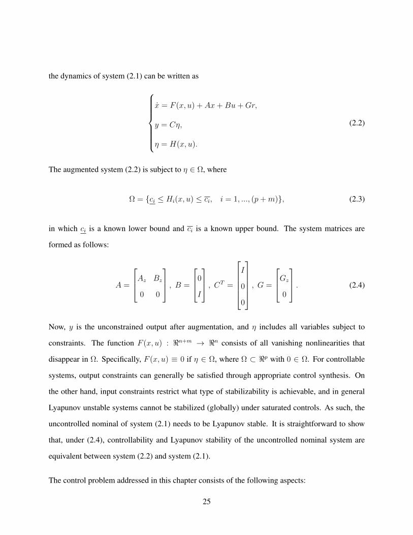
the dynamics of system (2.1) can be written as
x = F (x, u) + Ax+Bu+Gr,
y = Cη,
η = H(x, u).
(2.2)
The augmented system (2.2) is subject to η ∈ Ω, where
Ω = ci ≤ Hi(x, u) ≤ ci, i = 1, ..., (p+m), (2.3)
in which ci is a known lower bound and ci is a known upper bound. The system matrices are
formed as follows:
A =
Az Bz
0 0
, B =
0
I
, CT =
I
0
0
, G =
Gz
0
. (2.4)
Now, y is the unconstrained output after augmentation, and η includes all variables subject to
constraints. The function F (x, u) : <n+m → <n consists of all vanishing nonlinearities that
disappear in Ω. Specifically, F (x, u) ≡ 0 if η ∈ Ω, where Ω ⊂ <p with 0 ∈ Ω. For controllable
systems, output constraints can generally be satisfied through appropriate control synthesis. On
the other hand, input constraints restrict what type of stabilizability is achievable, and in general
Lyapunov unstable systems cannot be stabilized (globally) under saturated controls. As such, the
uncontrolled nominal of system (2.1) needs to be Lyapunov stable. It is straightforward to show
that, under (2.4), controllability and Lyapunov stability of the uncontrolled nominal system are
equivalent between system (2.2) and system (2.1).
The control problem addressed in this chapter consists of the following aspects:
25

• Stability conditions are derived for nonlinear system (2.1), its control design, and its robust-
ness in the presence of forecasting error (r − r).
• An optimal tracking control is developed for system (2.1) with respect to performance index
J =1
2yTf Sf yf +
1
2
∫ tf
t0
[yTQy + uTRu]dt, (2.5)
formed from similar terms in (1.5) and (1.6), where yf = Cx(tf ), Sf = S(tf ) ≥ 0. The
terminal conditions at tf are to be decided during the design process. A design based on
Lemma 3 and optimal control formulation (1.10)-(1.13) is presented to force the nonlinear
system to move into and remain in set Ω, which is explicitly constructed for systems with
saturations on the state and control.
• By embedding the optimal tracking control law in the barrier control design, constraints are
imposed to handle the system’s reactions to discrepancies in r(t) and r(t).
In this section, a general nonlinear control design is presented for system (2.1), and the correspond-
ing stability condition shown in Lemma 3 is utilized.
Inherently, Lemma 3 yields a more straightforward approach to apply the standard Lyapunov sta-
bility result to Jacobian systems derived from the original nonlinear system without loss of gener-
ality. In the case where V is quadratic, the property of Lemma 3 is used to construct the following
theorem, restated from [21] for convenience:
Theorem 1 Consider system (2.1) under control
u = −R−1BT (k(x, t)− v(r, t)), (2.6)
26

where v is a uniformly bounded function of r and time. If matrix
Γ(w) , S + S 5w [F (w) + Aw −BR−1BTk(w, t)]
+5w[F (w) + Aw −BR−1BTk(w, t)]TS
is positive definite for all w ∈ <n, then system (2.1) under control (2.6) has the following proper-
ties:
• If r = r, the state is asymptotically convergent to equilibrium state xe described by
xe = [F (xe) + Axe −BR−1BTk(xe, t)]
+BR−1BTv(r, t) +Gr. (2.7)
• If r 6= r, the tracking error is input-to-state stable with respect to forecast error (r − r).
Proof: Under control (2.6), system (2.1) becomes
x = [F (x) + Ax−BR−1BTk(x, t)] +BR−1BTv(r, t) +Gr.
If r = r, the trajectory of equilibrium state xe is governed by (2.7). Conversely, if r 6= r, then for
the state error e = x− xe, we have the error system
e = [F (x)− F (xe) + Ae
+BR−1BT (−k(x, t) + k(xe, t))]
+BR−1BT (v(r, t)− v(r, t)).
27
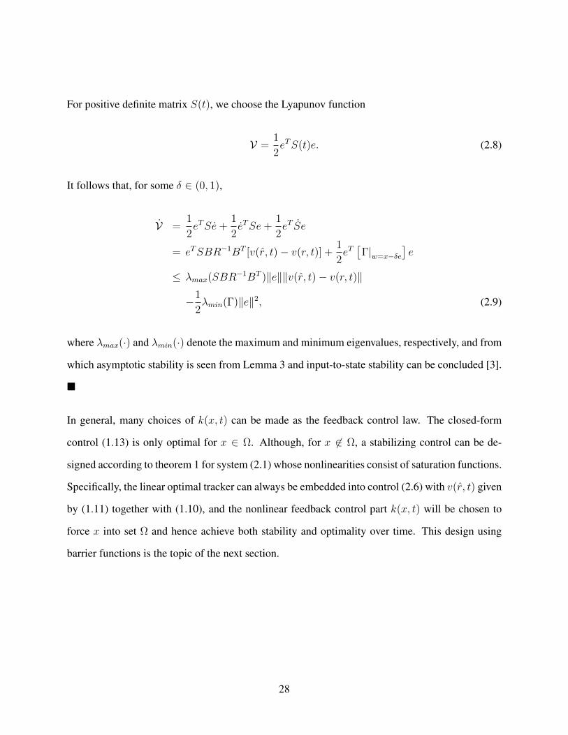
For positive definite matrix S(t), we choose the Lyapunov function
V =1
2eTS(t)e. (2.8)
It follows that, for some δ ∈ (0, 1),
V =1
2eTSe+
1
2eTSe+
1
2eT Se
= eTSBR−1BT [v(r, t)− v(r, t)] +1
2eT[Γ|w=x−δe
]e
≤ λmax(SBR−1BT )‖e‖‖v(r, t)− v(r, t)‖
−1
2λmin(Γ)‖e‖2, (2.9)
where λmax(·) and λmin(·) denote the maximum and minimum eigenvalues, respectively, and from
which asymptotic stability is seen from Lemma 3 and input-to-state stability can be concluded [3].
In general, many choices of k(x, t) can be made as the feedback control law. The closed-form
control (1.13) is only optimal for x ∈ Ω. Although, for x 6∈ Ω, a stabilizing control can be de-
signed according to theorem 1 for system (2.1) whose nonlinearities consist of saturation functions.
Specifically, the linear optimal tracker can always be embedded into control (2.6) with v(r, t) given
by (1.11) together with (1.10), and the nonlinear feedback control part k(x, t) will be chosen to
force x into set Ω and hence achieve both stability and optimality over time. This design using
barrier functions is the topic of the next section.
28

Barrier Function Design
A barrier function is a representation of algebraic constraints on the output. In particular, any
bound on a state variable will be imposed as a barrier function, and the control forces the state into
set Ω. By nature, such a design ensures stability and, by making Ω an invariant set, control (1.11)
is applied within set Ω to achieve optimal performance.
Applying Definition 6, the relative degree can be found between the barrier function ξi(x) and
control input u. Using the concept of relative degree, for differential operator s, we can write
high-order time derivatives of ξi(x) as:
ξ(j)i (x) , sjξi(x) = L(j)
f ξi(x), j = 1, ..., µi − 1; (2.10)
and
ξ(µi)i (x) , sµiξi(x) = L(µi)
f ξi(x) +∂
∂x[L(l−1)
f ξi(x)]Bu. (2.11)
The following lemma based on the comparison theorem provides the mechanism of embedding a
set of barrier functions, denoted by ξi(x) ≤ 0 for i = 1, · · · , p, into a control design. By abuse
of notation, ξi(t) = ξi(x(t)). From (1.15) and the feedback linearization process, the following
lemma from [21] generalizes the equation to inequalities.
Lemma 4 Consider the following differential inequality:
µi∏j=1
(s+ γij)ξi(t) ≤ 0, (2.12)
where γij > 0 are constants. Then, solution ξi(t) has the property ξi(t) ≤ 0 for all the time
29

provided that ξi(0) ≤ 0, and
k∏j=1
(s+ γij)ξi(t)
∣∣∣∣∣t=0
≤ 0, ∀k ∈ 1, · · · , µi − 1, (2.13)
If ξi(0) 0, then ξi(t) ≤ 0 becomes true exponentially, given inequality (2.12).
Proof: Let
α0 = ξi(t), α1 = (s+ γi1)ξi(t),
and
αj = (s+ γij)αj−1, j = 2, · · · , µi. (2.14)
Then, differential inequality (2.12) can be expressed as
αµi = (s+ γiµi)αµi−1 ≤ 0,
in which u is present and can always be enforced by design. Now, consider whether αl(0) ≤ 0
implies αl(t) ≤ 0 and whether
(s+ γil)αl(t) = αl+1(t) ≤ 0. (2.15)
Upon analyzing the solution to the above differential equation: for l = µi − 1, · · · , 1,
αl(t) = αl(0)e−γilt + e−γilt∫ t
0
eγilταl+1(τ)dτ, (2.16)
it can be seen that it is valid. The lemma is proven by using the above result to differential equation
(2.15) recursively, from which non-positive values can be concluded from αµi(t) to αµi−1(t) and
recursively down to α0.
30

When ξi(0) 0, inequality (2.13) may not hold, however, we know αµi(t) ≤ 0 can be satisfied
with a proper choice of u regardless of whether αl(0) ≤ 0 for any l, thus, the integral term in solu-
tion (2.16) is negative and non-increasing, which in turn dominates the decrescent initial condition
term for each αl(t). Therefore, ξ(l)i (t) decreases exponentially.
Remark: If µi = 1, then (2.13) is not needed, and only ξi(0) can be verified, since from (2.11) and
definition 1, ∂∂x
[L(0)f ξi(x)]Bu 6= 0.
The specific steps of designing a successful barrier control are as follows:
Step 1: It follows from (2.3) that there are a total of 2p constraints and their corresponding barrier
functions are:
ξ2i−1 = Hi(x)− ci, ξ2i = ci −Hi(x), i = 1, · · · , p.
Determine the relative degree µi for each ξi.
Step 2: Choose positive constants γij for j = 1, · · · , µi and calculate the corresponding character-
istic polynomial:
∆i(s) ,µi∏j=1
(s+ γij) = sµi +
µi−1∑j=0
βjsj. (2.17)
It follows from the above expression, equation (2.11) and definition (2.14) that
αµi =∂
∂x[L(µi−1)
f ξi(x)]Bu+ L(µi)f ξi(x) +
µi−1∑j=0
βjL(j)f ξi(x).
Step 3: We know from Lemma 4 that barrier ξi(x) ≤ 0 can be ensured under differential inequality
(2.12) even when ξi(0) 0, which in turn is guaranteed by choosing the barrier control as
∂
∂x[L(µi−1)
f ξi(x)]Bu ≤ −
[L(µi)f ξi(x) +
µi−1∑j=0
βjL(j)f ξi(x)
]. (2.18)
31

Step 4: Given that the inequalities in Step 3 may admit many solutions of u, hence the best control
in the whole state space is given by the following real-time optimization problem:
u = argminu ‖u− u∗‖2 (2.19)
subject to inequality (2.18) for i = 1, · · · , 2p,
where u∗ is given by (1.13).
In fact, if u and u∗ evolve according to the same time scale and all constraints are enforced, Step 4
is not required, and if implemented it may actually slow down the calculation of input values when
the time increments are small. Step 4 is useful if there is significant delay in update rates for either
u or u∗, or if r and r are significantly different.
Theorem 2 [21]:Consider system (2.2) with A′ being Lyapunov stable and pair A′, B′ being
controllable. Suppose that the augmented nonlinear system (2.1) with “output” ξi is input-output
feedback linearizable of relative degree µi and with Lyapunov stable internal dynamics [3]. Then,
nonlinear system (2.1) is controllable, it has a Lyapunov stable nominal system, and tracking
control (2.19) is stabilizing for all feasible reference signal r(t) and with its (good) forecast r(t).
If r(t) is close to r(t) and if control (2.6) with v(r, t) renders that u′ stays within its bounds, the
control is also optimal.
Proof: It follows from (2.4) that A is Lyapunov stable if and only if A′ is Lyapunov stable and that
A,B is controllable if and only if A′, B′ is controllable. Hence, linear optimal control u∗ in
(1.13) is stabilizing for nonlinear system (2.1) whenever F (x) = 0. In the region that F (x) 6= 0,
the barrier controls in (2.18) and the optimized version obtained from (2.19) are stabilizing controls
and both force x into Ω exponentially as shown in Lemma 4.
32

Application of Theorem 2 involves dynamic inversion, which holds for general nonlinear system
of form (2.1) provided that the system has controllable pair A,B, that its uncontrolled nominal
systems is Lyapunov stable, and that it is input-output feedback linearized with respect to the
constraints to be imposed. For those systems, Theorem 2 provides a real-time near-optimal control.
In Figure 2.1, a block diagram of the implementation structure is shown. In real-time, r is used to
synthesize the optimal control, which may be updated as often as a new forecast is acquired.
Figure 2.1: Barrier Function in Optimal Control Block Diagram
The following examples are included to illustrate details of the design steps.
Example 4 Consider the following system with output and state dynamics saturations:
x1 = x2 + u
x2 = −SAT±1[x1] + r
η = SAT±1[x1],
which can be written in the form of (2.1) with F (x) = x1−SAT±1[x1], A =
0 1
−1 0
, B = [1 0]T ,
G = [0 1]T , SAT±1[x1] = H(x). The objective of the control is to stabilize the oscillating dynamics
subject to the exogenous input, which may be considered as a reference signal that is susceptible
33

to disturbance. While the control is active, the state trajectory must remain within the set Ω, which
has the following structure:
Ω =
x ∈ <2 : −1 ≤ x1 ≤ 1
.
Tracking control (1.13) can be used to achieve an optimal trajectory. However, to ensure the
constraints are obeyed, the design is continued by determining relative degrees from Definition 6,
then forming the barrier control from αµ with βj = 1 ∀j as
u ≤ −x2 − (x1 − 1)
−u ≤ x2 − (−1− x1)
In real-time, optimization (2.19) is applied subject to the above constraints to achieve a near-
optimal trajectory.
Example 5 Consider the following system with input rate saturation:
z1 = z2
z2 = −z1 − 0.5z2 + u′ + r
uo = SAT±1[u]
yo = z1.
34

After augmenting, we arrive at:
x1 = x2
x2 = −x1 − 0.5x2 + x3 + r (2.20)
x3 = SAT±1[u]
where the initial condition vector is x0 = [1 1 1.1]T . The set Ω has the following structure:
Ω =x ∈ <3 : −1 ≤ u ≤ 1
.
It follows from Definition 6, Lemma 4, and (2.18), that the control barrier is
u ≤ 1
−u ≤ 1.
The dynamics of system (2.20) resemble that of a second order oscillator subject to a sinusoidal
exogenous input r. The objective of the control is to minimize the oscillations of the internal
dynamics of the system, that is, to force x1 and x2 to zero by using the augmented state x3, which
is controlled by u.
35

Figure 2.2: Control and State Trajectories of Input Rate Saturated System
We see that, in Figure 2.2, the states x1 and x2 do not converge to zero as desired due to the input
rate saturation. There are a few important points of interest that are present in these results:
• The initial condition of u is outside the barrier but is immediately forced within the bounds
by the design.
• Although the original internal state dynamics are not saturated, the input rate saturation
alone causes the entire system to oscillate.
• When r is relatively large and fast, the rate-limited control cannot keep up, therefore, opti-
mality is compromised.
• Even through state augmentation, x3 is the original control to be designed, but since the
augmented control (or rate of x3) u is saturated, the speed of x3 is too slow.
36

If such a signal is provided that the system is incapable of handling with respect to operation speed
and constraints, then the signal r may be considered infeasible, which is the exception for Theorem
2.
Imposing the original constraints as barrier functions allows us to determine a solution that re-
mains within the given state and input limits. Because the trajectory of r is an estimation, the true
trajectory of r can effect dynamics differently than expected. In real-time, the nonlinear control
can compensate for cases where r 6= r. The linear optimal solution pair of x∗, u∗ is obtained by
including r as the reference, not r, so it is necessary to correct any disturbances produced by the
real-time reference r. Standard optimal control procedures are only optimal if the system trajec-
tory does not deviate from the solved trajectory of x∗ when u = u∗. Thus, a real time solution is
provided to guarantee the state and control trajectories remain optimal or close to optimal. Updates
in the estimated reference signal drive adaptation of the barrier, such that a better estimation allows
for increased performance.
Summary
A generalized nonlinear control was designed for systems with input rate and input/output mag-
nitude limits. The design imposes constraints in real-time by using a barrier function formulation
along with input-output feedback linearization. Although saturations are the only static nonlinear-
ity included in the form of existing system constraints, the nature of the barrier function formula-
tion allows any nonlinearity to be modeled within the barrier function. The result is a slightly more
complicated calculation of the barrier function polynomial, in which multiple derivatives of other
nonlinearities may not lead to equaling zero. Embedded in an optimal tracking control, the con-
trol design ensures that constraints are satisfied while achieving optimal performance subject to an
unknown exogenous input. In practical systems, exogenous inputs resemble real-time data being
37

gathered. Typical designs may not consider discrepancies between the real-time exogenous input
and the estimated value, which can lead to stability problems in sensitive situations. Optimizing
trajectories based on estimated data while ensuring that constraints are satisfied by real-time data
provides an encompassing solution for maintaining performance and safety. Applications which
involve forecast-dependent control meld well together with the design discussed in this chapter,
especially when forecasts are not completely accurate.
The scenario of microgrid power control lends itself to the usage of the barrier design structure with
a known (and feasible) but not guaranteed estimation r, which is discussed in the next chapter.
38

CHAPTER 3: MICROGRID CONTROL WITH HIGH-PENETRATION
OF PHOTOVOLTAICS
As the structure of modern microgrids becomes more complex, there is a greater need for advanced
control techniques to address important issues such as power balance and system stability, customer
satisfaction, and optimal operating costs. Although large-scale renewable generation proves to be
an effective power contributor, it can have adverse effects in regards to traditional generation and
frequency stabilization. High penetration of renewables can cause major power swings which
require governor actions that stress existing components in traditional generation.
A common solution to assist in balancing power in distributed energy resources (DER) is by forced
reduction of generation from renewables, or curtailment, which is extremely costly and sometimes
ineffective [37]. In [38], a thorough overview of DERs in microgrids is presented, and the difficul-
ties of grid integration and maintaining system stability are addressed.
In a microgrid, frequency deviation can occur due to the intermittent nature of renewable genera-
tion. Higher penetration of renewables can lead to larger frequency deviations, and can possibly
destabilize the microgrid if not handled accordingly. To avoid destabilization and minimize fre-
quency deviations, battery energy storage systems (BESS) and demand response (DR) must be
utilized properly. However, since traditional generation, battery operation, and DR act at different
time scales, the coordination of each of these elements must be addressed carefully.
Additionally, the battery energy storage system (BESS) capacity must be determined. In [39], a
battery sizing strategy is proposed through a novel cost-benefit analysis, and further, in [40], a
detailed description of various types of energy storage systems is presented, although specifically
for wind power integration.
39

Similarly, controlling charging/discharging of the BESS has been addressed by many researchers.
A distributed control method is shown in [41] to regulate voltage in distribution networks with
high photovoltaics (PV) penetration. In [42], reactive power control is coupled with BESS control
to regulate voltage profiles in a residential distribution network setting; and the authors of [43]
present a frequency control strategy for three-phase BESSs. In [44], a survey of DR in smart grids
is presented along with scheduling, modeling, issues, and various solutions to those issues. More
specifically, the authors of [45] propose a distributed cooperative method to provide a load control
for ancillary services.
Using advanced techniques to control separate microgrid elements may not be enough when con-
sidering the diversity of devices and DERs present in the system without considering physical
interactions among devices. By implementing an optimal control that can handle constraints as
well as real-time disturbances can coordinate usage of multiple microgrid elements. In [1], a sim-
plified design of a locally coordinated optimal control is proposed, however, the design assumes
system constraints are satisfied so no nonlinear design was explicitly shown, and real-time distur-
bances could not be handled well. In [46], the authors propose a three-layer control strategy to
stabilize microgrid frequency, however, they aggregate renewable generation into electric power
without specified dynamics.
In the context of power systems, optimization and optimal control is mostly used on a higher level
of direct power control or distributed network control, and typically is not used to delve into sys-
tem dynamics for transient stability analysis due to the difficulties with existing methods. In [47],
an optimization problem is formed to determine the optimal power generation of each agent in a
power network, but does not consider specified generation sources and dynamics thereof. Also, in
[48], an optimal power flow control technique is employed by using Pontryagin’s minimum princi-
ple without considering the impact of dynamics. On the other hand, the authors of [49] considered
the notoriously problematic saddle point dynamics to develop an extremum seeking distributed
40

optimization in application to energy consumption in smart grids. However, in scenarios consid-
ering inter-area oscillations, dynamics of power generation are focused upon while integration of
renewables is aggregated [13].
State constraints in power systems are often considered when solving optimal power flow, however,
when real-time transient stability is in question, designs become much more complex. Various
works have investigated transient stability constrained optimal power flow [50], [51], but do not
consider fluctuations during transience. Common problem formulations such as solving optimal
power flow do not contain input or input rate constraints due to the lack of transient analysis since
the dynamics themselves are used as the constraint. Transient stability is explored in [52], where
oscillator-based synchronization of first order unconstrained models is shown.
Constrained Control in a Microgrid
This problem structure is directly applicable to power distribution systems, where r represents the
net load forecast. In this context, the objective is to balance load and generation through the use of
the control input. Typically, power systems have constraints that must be satisfied for safety and
performance reasons, such as frequency and turbine gate limits. More components are added in
modern microgrid structures, which also adds more constraints on the system. Including a BESS
and DR control capabilities adds system constraints of capacity limits and acceptable DR range,
respectively. Naturally, barrier functions are advantageous in this situation due to well-defined
boundedness while remaining continuous.
The coordination of the controls for traditional generation, BESS, and DR can be primarily done
by using a typical linear-quadratic optimal tracking control as long as the real-time reference r
does not deviate from the estimated r. The relative priorities or costs of utilizing each element can
41

be assigned parameters in the performance index, namely R, to minimize costs associated with
each power contributing component.
PV, Duck Curve, and Saturations
Disturbances in real-time cannot be easily reconciled in standard optimal control or typical power
systems, and can lead to destabilization of the system. Since tracking control is derived from
an open-loop method, when there are deviations in real-time, the solved trajectory is no longer
optimal. The open-loop portion of the design depends on an estimation, therefore, a base load
profile from [53] on January 1, 2017 is selected as the day-ahead load forecast, combined with
solar generation data from a test case in the software OpenDSS to craft a net load profile that
includes intermittent solar generation behavior, which is shown in Figure 3.1. When renewable
penetration is high, the net power consumption dips far below the base load during the middle of
the day. The shape produced looks similar to that of a duck, thus, such a load profile is commonly
referred to as a “duck curve.”
42

Figure 3.1: Sample Net Load Profile with Intermittent Solar Generation
In a modern microgrid, frequency stabilization and load balancing are main concerns. When in-
cluding the power contribution of DR and readily available battery energy in the microgrid, fre-
quency stabilization becomes more difficult, especially if local system objectives are prioritized
without coordination. The model of a microgrid can be presented as a series of first order differen-
tial equations that are coupled through state feedback. The state equation representation illustrates
how each control input should be designed to effect power generation.
Traditional generation is often represented by the swing equation:
Mω = −Dω + Pm − Pb − r − Pdr, (3.1)
where M is the generator inertia constant, ω is frequency, D is the generator damping, Pm is
mechanical power, Pb is battery power, and Pdr is the consumer load from demand response. While
43

r still signifies a reference to be tracked in system (2.1), here it represents the net load forecast.
Intuitively, the amount of power generated should equal the net load for optimal performance.
Each of the power generating components have individual first or second order dynamics relative
to the control input. The control for traditional generation is implemented in the governor dynamic
equation in the form of:
Mgxg = −xg + ug, (3.2)
whereMg is the governor inertia constant, xg is governor state signal, and ug is the governor control
signal. The relationship between the governor control and power generation can be described by
the mechanical power dynamic equation:
MsPm = SAT(xg − Pm), (3.3)
where Ms is the inertia constant. The rate of mechanical power generation is limited by the satu-
ration in (3.3). Typically, this physical constraint is called the ramping rate, and can be related to
the rate of valve operations for the governor and turbine [54].
Demand response dynamics have a direct first order relationship with its control input, as shown
in the following equation:
MdrPdr = −Pdr + udr, (3.4)
where Mdr is considered as a time constant, and udr is the DR command signal. Due to the sign
definition of Pdr in (3.1), a positive value indicates that DR is absorbing power. Here, we assume
that power from DR is always possible to control if needed. Of course, this assumption does not
consider consumer decisions involving price dynamics or incentives, which is beyond the scope of
44

this topic.
The final two dynamic equations are related to the BESS and are presented below:
τ Pb = −SAT[ub], (3.5)
E = Pb, (3.6)
where τ is a time constant, ub is the battery power command signal, and E is the battery energy
state. Since the rate of charging and discharging can change much faster than traditional gener-
ation, the time constant τ is much smaller than M . The capacity limit on E does not depend on
dynamics, although it is important to determine the minimum acceptable value as well as the min-
imum required capacity. Due to the sign definition in (3.1), a positive value of Pb results in the
battery charging, which constitutes a loss of available generation.
The constraints on specified system states to ensure safe power system operation are presented
below in a compact form:
|SAT(xg − Pm)| ≤ us (3.7)
−0.05 ≤ ω − ω0 ≤ 0.05 (3.8)
|Pdr| ≤ Pdr (3.9)
0 ≤ E ≤ E, (3.10)
where us is defined as the ramping rate limit. Typical frequency deviation limits are within 5%
of nominal values; and we allow the minimum energy of the battery to be zero. The required
DR should be limited by an upper bound of Pdr to ensure that customer action is not necessarily
required, but commands can be issued if needed. Constraints (3.7)-(3.10) are imposed by the
barrier function design using the results in the previous chapter.
45

If the traditional generation maximum ramping rate is not large enough, the generation will lag
behind the net load, which can cause large deviations in frequency. An estimate of the maximum
required ramping rate can be gathered from the net load envelope, not considering intermittent
renewable generation. This can simply be done by calculating the approximate slope of the duck
curve during the largest ramping phase, which can be seen approximately between 12:00 and 18:00
in Figure 3.1, and making sure that traditional generation alone can achieve that slope.
Figure 3.2: Trajectory of ug and its Limiting Values
Figure 3.2 shows the trajectory of ug as well as the limiting values of ug, which are calculated
from barrier functions formed according to constraint (3.7). It is apparent that, during the periods
of the net load profile changes rapidly, control ug makes the ramping rate reach but not exceed its
boundary. Nonetheless, ug is incapable of compensating for the large swings in PV generation due
to the ramping rate limits.
The upper bound of the battery energy can be determined based on solar firming shown in the
46

following equation:
E =
∫ tf
0
(r − Pr(t))dt. (3.11)
However, is important to determine the lowest battery capacity needed in order to help minimize
the required cost of the BESS. This type of firming procedure is done by integrating the difference
in the net load forecast and the actual solar generation. This calculation takes into account the
variability of solar, in which it is best to assume a highly intermittent case, where Pr(t) is the
“worst-case” past solar data in the region.
Figure 3.3: Difference in Forecast vs. Actual Net Load due to Solar Generation
In Figure 3.3, the difference between net load and the load envelope is shown. Due to the penetra-
tion level of solar in this case, large fluctuations in power occur, and can reach beyond 0.7 per unit
in a short amount of time. These differences can be captured by integration, which allows us to
47

determine the maximum required battery capacity. In Figure 3.4, the integration of the difference
in net load and the load envelope is shown. Thus, a safe choice for the battery capacity would
be E = 0.3 if only the BESS is used for these sharp changes in load. Additionally, the energy
calculation in (3.11) does not consider the fact that the battery can be charged from a temporary
excess in traditional generation, so the chosen value of 0.3 can be treated as highly conservative
capacity.
Figure 3.4: Integration of Difference in Forecast vs. Actual Net Load
Since machine inertia plays an important role in microgrids, whether physical or virtual, as shown
in [55], some portion of traditional generation can cover the low frequency variations in renewable
intermittency. Also, we can attribute some generation to DR by reducing loads, such that we may
greatly reduce the required capacity of the BESS.
Additionally, knowledge of r is advantageous in determining a smaller battery capacity than what
firming can provide. An offline simulation can be performed and tuned using the linear optimal
48

tracker (1.10)-(1.13) and can even include the past solar data Pr. From this reasoning, with the
inclusion of DR and the effect of inertia, we choose the BESS capacity as E = 0.07.
Simulation and Discussion
By coordinating the usage of traditional generation, DR, and BESS, the microgrid can success-
fully provide power to consumers while maintaining an operational status within the boundaries of
safety and performance. Different power contributing elements have different effects on the micro-
grid, and can be handled by the proposed control design. The impact of each component is shown
through simulations in various scenarios. For all cases, the optimal tracking parameter matrices are
chosen as R = diag1, 20, 10 for the control vector [ug udr ub]T and Q = diag0, 500, 250, 200
for the output vector y = [(xg − Pm) ω Pdr E]T .
Each power generating or power consuming component has an impact on stabilizing system fre-
quency. Obviously, the goal is to minimize the deviation of frequency from nominal. The most
straightforward way to achieve this in the design is to penalize deviations within the optimal track-
ing control, however, this may lead to other state variables not being penalized enough. Typically,
the safe range of operation for the system frequency is within 5% of nominal, so we shall deem
anything beyond a 0.05 per unit deviation unacceptable.
As an important parameter, ramping rate limits can cause frequency deviation when the traditional
generation rate is saturated. With inertia constants of M = Ms = Mg = 1, the operational speed
of traditional generation is relatively slow. To gain an understanding of the effect of ramping rate
limits, DR and BESS are inactive at this point. In Figure 3.5, it can be seen that when the net load
exhibits large swings, traditional generation cannot keep up with the change, so the frequency rides
on the bounds. This is due to the maximum ramping rate of us = 0.1.
49
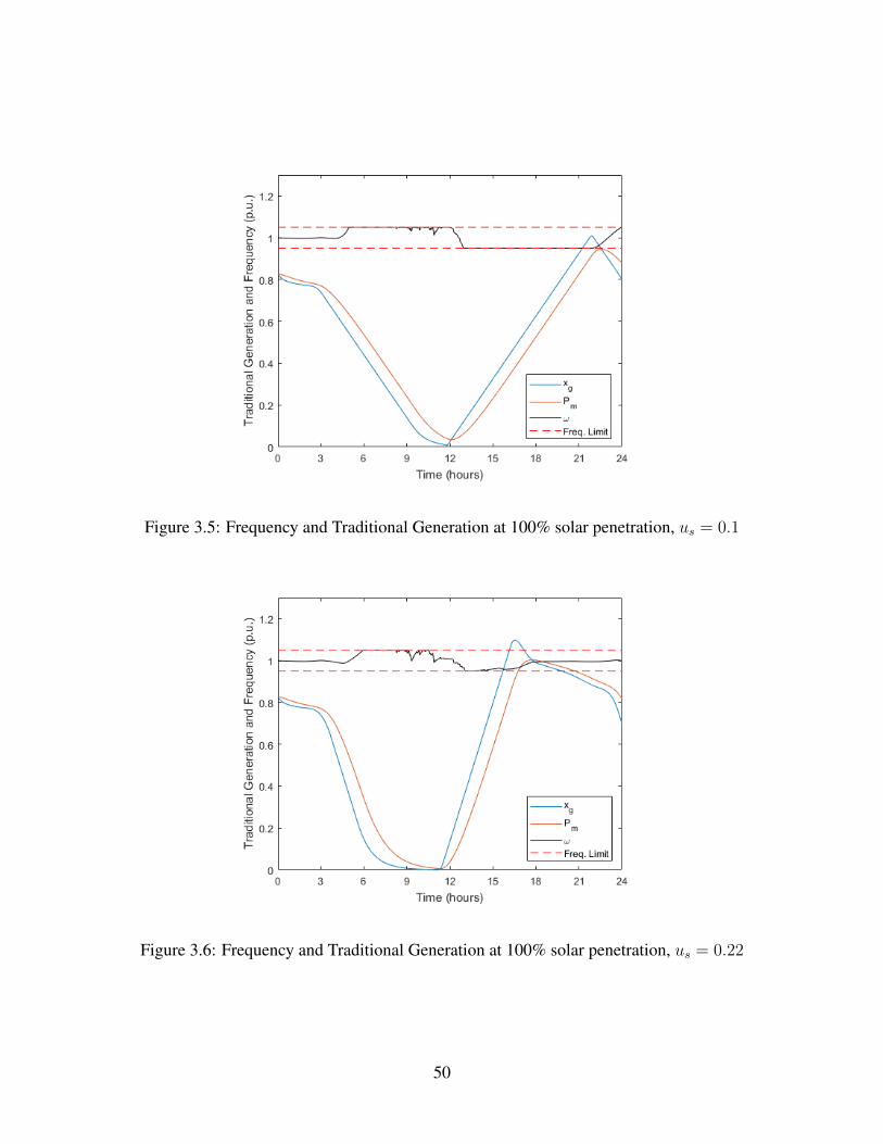
Figure 3.5: Frequency and Traditional Generation at 100% solar penetration, us = 0.1
Figure 3.6: Frequency and Traditional Generation at 100% solar penetration, us = 0.22
50

In such a system with 100% renewable penetration, a low ramping rate limit does not allow tra-
ditional generation to react fast enough to the net load envelope. By allowing a higher maximum
ramping rate, traditional generation alone can be fast enough to cover the large net load variations,
and thus allows the frequency to remain closer to nominal, or at least keeps the frequency from
riding along the bounds, which can be seen in Figure 3.6. Even though the governor signal xg
reaches zero, the mechanical power value Pm does not.
Choosing the BESS capacity too large can be wasteful, however, it is important to understand what
is required based on the other power sources in the microgrid. With time constants Mdr = 0.1 and
τ = 0.01, operational speeds of DR and the BESS are approximated as ten times and one hundred
times faster than traditional generation, respectively. In Figure 3.7, while the ramping rate limit
remains at 0.1, the battery energy is saturated, and DR reaches the limit. From this behavior, we can
conclude that BESS and DR will not have a significant impact on frequency stability if traditional
generation cannot follow the net load envelope. A possible but not recommended solution is to
increase the BESS capacity. To illustrate this further, Figure 3.8 shows the traditional generation
and frequency of the case where BESS and DR are active.
Thus, in this case, not even firming is a valid solution if the BESS is the only component capable of
handling net load changes due to renewables, although the frequency stability problem still exists.
However, the saturation of BESS is primarily due to the level of renewable penetration, not the
intermittency.
If there is a larger ramping rate limit, frequency deviations are reduced, however, with only the
BESS contributing to counteract such large changes in net load, the frequency performance is not
yet at a desirable stage. In Figures 3.9 and 3.10, by prescribing us = 0.22 and keeping the battery
capacity at E = 0.3, the contribution of the BESS is not enough to have a significant effect on
frequency stabilization.
51

Figure 3.7: Stressing BESS and DR Behavior due to Low Ramping Rate Limit, us = 0.1, E = 0.3
Figure 3.8: Frequency and Traditional Generation, us = 0.1, with BESS and DR, E = 0.3
52

Figure 3.9: Frequency and Traditional Generation, us = 0.22, with BESS, E = 0.3, without DR
Figure 3.10: BESS Behavior without DR, E = 0.3
53

Figure 3.11: Frequency and Traditional Generation, us = 0.22, with BESS, E = 0.07, and DR
Figure 3.12: Optimal BESS and DR Behavior, E = 0.07
54

Frequency becomes easier to deal with when traditional generation is fast enough to cover the net
load envelope, which allows the BESS and DR to focus on handling intermittent behavior and
excess generation. In Figures 3.11 and 3.12, the frequency performance is substantially better
with both BESS and DR. Additionally, since DR is included, the BESS capacity needed is 0.07.
Ultimately, available operation of both BESS and DR allows the storage capacity to be drastically
reduced while stabilizing frequency even more. Since DR is capable of operating on a time scale
in between traditional generation and the BESS, it can assist in both regards.
There is a natural trade-off between BESS and DR usage, since both can directly contribute to
highly intermittent behavior of renewables. The penalties on either can be customized in the off-
line optimal tracker according to microgrid requirements. Since DR remains positive for the major-
ity of time during the day, consumers are required to use more load, which is more acceptable than
requiring consumers to reduce loads. Of course, the usage of more load during the solar peak hours
can be encouraged through incentives, but this concept is beyond the scope of this dissertation.
Summary
The optimized control presented in chapter 2 is applied in a modern microgrid environment with
various power generating and power consuming elements. By optimally coordinating these el-
ements, the novel control design successfully stabilizes and balances loads subject to input rate
and input/output magnitude saturations. Simulation results show relationships between specified
capacity limits and available generation, and their impact on system stability. Ultimately, the op-
timal capacities of microgrid elements are determined through simulations while satisfying all
constraints in real-time subject to disturbances due to intermittent PV generation. Thus far, coordi-
nation of modern grid elements with existing traditional generation has been addressed, however,
in the absence of traditional generation, inverter-based designs inclusive of grid-forming structures
55

require more attention. As smaller but numerous distributed energy resources become more promi-
nent in designs over large centralized traditional generation, machine inertia can no longer be relied
upon to anchor the system despite quick power fluctuations, and wide-area stabilization and con-
trol becomes the focus rather than local controls. Theoretically, the advantages of passivity-short
network properties can be exploited to contribute to such distributed systems, especially when in
combination with utilizing HW model identification for complex power elements.
56

CHAPTER 4: NONLINEAR AUTOPILOT DESIGN
Applications in which practicality is of utmost importance lie in aerospace. With highly nonlin-
ear dynamics and numerous explicit constraints, control designs for aerospace applications are
generally challenging. When designing controls with the possibility of real implementation, lin-
earization techniques and approximations are sometimes used although stability and performance
may be compromised in certain stressing situations. Given the highly nonlinear and coupled dy-
namics of typical aerial vehicles, the process of designing stabilizing controllers can be done while
simplifications are made. Usually such designs involve small angle approximations or lineariza-
tion around an equilibrium point or multiple points. These approximate control designs may be
sufficient for specific applications where states or trajectories are guaranteed to fall within the lin-
earized system domain. In the presence of input and output constraints, many existing control
methods must be highly customized. Many existing nonlinear control techniques can be tedious,
involving differentiation of unknown variables in which approximation can serve its purpose.
Designs including real-time parameter estimation from a linear model reference have contributed
to improve performance of 6 degree-of-freedom vehicle simulations [56]. However, when vehi-
cle motion exceeds the expected range of maneuverability, control designs based on small angle
approximations are no longer effective. In [57], the authors design a complex three-layer con-
trol based on a simplified model that categorizes velocity changes as uncertainties. Although their
design is highly detailed, simulation results show that there is difficulty in reference tracking. Non-
linear control techniques were used in [58], but constraints were applied as saturations directly in
the simulation without control compensation.
In this chapter, a novel nonlinear control design is used to maneuver a 6 degree-of-freedom hypo-
thetical vehicle with constraints applied through the barrier function design.
57

Problem Formulation
Consider the following equations of motion:
VB =1
m(FB − mVB)− ωB × VB (4.1)
ωB = J−1B (MB − JBωB − ωB × JBωB) (4.2)
where subscript B signifies the Body reference frame, VB = [u v w]T is the translational velocity
vector, ωB = [p q r]T is the rotational velocity vector, m is the vehicle mass, FB is the translational
force applied, MB = [MR MP MY ]T is the rotational force applied, and JB is the inertia matrix
of appropriate dimension. It should be noted that m may be considered as zero in implementation
even in the presence of variable mass due to the discrete nature of simulation and practical imple-
mentation. Instead, values of mass can simply be updated at each discrete-time step in practice
without needing a differential. The same can be true for JB.
The goal is to design a fully nonlinear translational acceleration autopilot control, where the only
control surface is through momentMB. Typically, one may take the derivative of (4.1) and approx-
imate unknown terms, or make assumptions on small angles for the pointing direction of velocity
versus the x-axis body frame (known as the angle of attack, α, and sideslip, β). Enforcing small
angle dynamics is not guaranteed automatically, so barrier functions may be used to manually
impose constraints on α and β.
It is assumed that only the pitch and yaw moments can be controlled, therefore, it is assumed that
p = p = 0. Suppose it is desired to constrain incidence angles α and β such that a linearized
model could be used for dynamic simulations. Physically assuming α and β are small means that
58

commands issued to the control surface are also small. The idea is to minimize instantaneous angle
changes, which is equivalent to minimizing instantaneous velocity changes along the y and z axes,
which can be seen according to (4.3). Therefore, an acceleration control could be put to best use.
αβ
=
tan−1(wu
)sin−1
(v‖VB‖
) (4.3)
In Figure 4.1, coordinate frame sign conventions as well as angle definitions are shown. The
incidence angles are calculated from the labeled body velocity components w and v.
Figure 4.1: Coordinate Frame and Angle Convention for Aerial Vehicles with Canards
Aerodynamics govern the rotational motion of the vehicle since the control surfaces are the ca-
nards. The angle of the canards is denoted as δ, which can be decomposed into components δP
and δY signifying pitch and yaw deflection angles, respectively. The following equations show a
59

hypothetical relationship between canard angles and aerodynamics:
δP =1
d1
[1
qSref lrefMd
P − (c1α3 + c2α|α|+ c3α + c4α|β|)
],
δY =1
d1
[1
qSref lrefMd
Y − (c1β3 + c2β|β|+ c3β + c4β|α|)
],
where Sref and lref are known area and length, q is dynamic pressure, and d1, c1, c2, c3, c4 are
coefficients determined from parameters. The process of imposing constraints to ensure small
angle approximations are valid is shown in the following section.
Nonlinear Control for Autopilot
Dynamic equations (4.1) and (4.2) are each first order, however, they are coupled through ωB×VB,
which means MB is part of the inner loop control input, and FB is part of the outer loop control
input. For notational purposes, MdB and F d
B will be the inputs to design, while MB and FB are
the leftover moments and forces due to aerodynamics. The relationship between the control loops
and aerodynamics is kinematic, which means effort will only be required for designing two control
input vectors.
Reflecting an output from guidance, a desired translation acceleration command V dB is provided.
For convenience, system (4.1) can be represented as:
vw
= A+B
qr
, (4.4)
where A = 1m
(FB − mVB) and B =
0 −u
u 0
. Then, the control design based on backstepping
60

is applied to obtain nonlinear expressions for qd and rd, which serve as the outer loop control.
Usually for nominal flight trajectories, angle of attack and sideslip should not be large. Exceptions
to this include vehicles designed for high-maneuverability, which takes advantage of the fact that
the vehicle structure can withstand high values of angle of attack and sideslip. For part of the
current study, it is assumed that constraints bound both angles as constants according to:
α ≤ α ≤ α, β ≤ β ≤ β.
The above constraints are imposed by the use of barrier functions within the outer loop control.
Details of the development are provided in Appendix B for authorized readers.
Continuing to design the inner loop control results in a nonlinear expression for the vector MdB
which stabilizes the system in closed loop. If desired, one can apply the same method to impose
constraints on canard angle deflection, although some observer estimations are required due to
unknown derivatives.
Software Framework
Implementation of the outer and inner loop controls is done in the Autopilot block in the simula-
tion structure in Figure 4.2, which was originally provided as an academic model. Other blocks
include dynamics with aerodynamics, actuators, and modeled measurement devices. The novel
autopilot design is implemented in the Autopilot block, and details of implementation are shown
in Appendix B.
61

Figure 4.2: 6 Degree-of-Freedom Aerial Vehicle Simulation Block Diagram
In order to verify the utility of the proposed control design, two sets of simulations are performed.
The first set of results are shown in Figures 4.3-4.5, which are simulated without constraints on α
and β, while the second set of results shown in Figures 4.6-4.7 include constraints of 5 degrees
for each channel. From each result, it can be seen that from dynamic coupling between the y
and z body axes, a movement in one axis causes motion in the other axis. Although usually this
is undesirable, it is also unavoidable in practice due to asymmetric mass distribution, which is
equivalent to possessing inertia matrices that are not simply diagonal matrices.
62
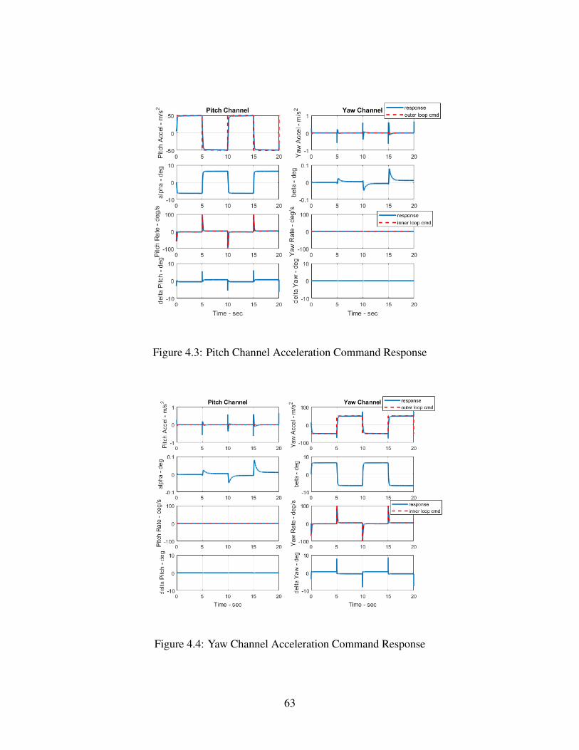
Figure 4.3: Pitch Channel Acceleration Command Response
Figure 4.4: Yaw Channel Acceleration Command Response
63

Figure 4.5: Simultaneous Pitch and Yaw Acceleration Command Responses
Dynamic coupling, along with relatively high control gains for speed cause small spikes when
commands change drastically. In the single channel test results shown in Figures 4.3-4.4, the
command is switched to ±50 m/s2 every 5 seconds, then in the simultaneous command results
shown in Figure 4.5, the frequency of changes for each channel is different.
In Figure 4.6, it can be seen that the acceleration response does not reach the command signal
because of the constraints on α and β. While imposing these constraints may provide a more
accurate model if small angle approximation is used on incidence angles, the overall performance
may suffer due to the magnitude and speed of fluctuation of given commands. This concept is
tied in with the previous chapter’s concept of a feasible reference signal. Although such stressing
maneuvers are excellent choices for model and control validation, angle constraints must not be
forgotten when angle dynamics are approximated.
64

Figure 4.6: Acceleration Response with Constraints Imposed on α and β
HW Modeling
Although the simulated vehicle has explicit dynamic equations which govern its behavior, in reality
the governing dynamics or a part thereof may be unknown. If dynamics are unknown, but input
and output data can be measured, then the dynamic model can be estimated by model identification
techniques. Since we have applied constraints on certain states, we have created nonlinearities that
must be taken into account. The Hammerstein-Wiener model fits this structure well. Results of HW
identification vary based on what is being analyzed, even in the same system. After applying the
HW approach to a single channel while unconstrained, the pitch acceleration results are presented
in Figure 4.7, with a 99.34% match. This means that under the step-type commands given, it is
expected that 99.34% of the output data in the approximated model will match the actual model
65
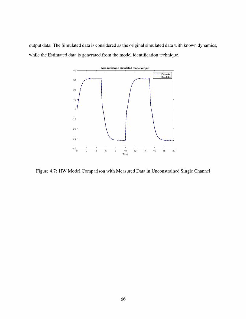
output data. The Simulated data is considered as the original simulated data with known dynamics,
while the Estimated data is generated from the model identification technique.
Figure 4.7: HW Model Comparison with Measured Data in Unconstrained Single Channel
66

Figure 4.8: HW Model Comparison in Pitch Channel with Constraints
Figure 4.9: HW Model Comparison in Yaw Channel with Constraints
However, if we run the same model identification on separate channels while imposing constraints,
the results are less accurate. Since separate channels are dynamically coupled, this proves to be
67

a more challenging task to identify an accurate model. As shown in Figures 4.8 and 4.9, the
HW model does not fit the pitch and yaw channel acceleration data (respectively) as well as the
independent channel analysis. Although with a data match of 86.30% for pitch and 81.96% for
yaw, the identified model still provides reasonable behavior of the system.
It must be noted that model identification for control purposes is highly sensitive to input data.
For instance, if the command signal is changed to a sinusoidal signal, the model estimated from
using a square wave will most likely be inaccurate. The underlying goal of model identification for
control is not to create the highest quality model, but instead to obtain a model that is valid under
the given control or family of control inputs.
There are two methods of HW model identification that are used to produce the results shown in
Figures 4.7, 4.8, and 4.9. Both methods require the System Identification Toolbox available in
MATLAB/Simulink 2019. Shown below is the first method in which the function ‘nlhw’ in the
Toolbox is called in line 8, specifying saturations on both input and output.
Since by default, the HW model can identify other types of nonlinearities, specification is needed
for identifying saturations only. Options for optimization parameters can be assigned as necessary.
The output and input arguments refer to the measured data sets of the model which needs identifi-
cation. The argument ‘order’ refers to the number of poles the identified system will possess. An
example of usage in a MATLAB script file is shown below:
68

Here, the variables ‘pitchChannel’ and ‘yawChannel’ are stored as custom data structures specific
to the System Identification Toolbox. Here, body acceleration data is sent as the ‘output’ argu-
ment, and body acceleration commmands are sent as the ‘input’ argument. For validation, the data
structures ‘pitchChannel’ and ‘yawChannel’ can be navigated to locate the Linear Model parame-
ter matrices, to which the same control signals are applied. The original output is plotted against
the output of the obtained Linear Model output, and a comparison can be made.
The second method of using the HW model identification technique yields the same result as the
first method, but involves a graphical user interface instead of code. The user interface below
appears upon opening the System Identification Toolbox, or by entering ‘systemIdentification’ in
the MATLAB command window.
69

By navigating through the user interface, data can be imported (on the left) and identification
techniques can be chosen and configured (in the center) to obtain a final model (on the right).
More details can be found at https://www.mathworks.com/products/sysid.html.
Real-Time Data-Driven Modeling and Control
Using the same HW model identification process in real-time leads to an indirect adaptive method
that consists of two parts: First, input and output data is gathered and fed into the HW model
algorithm that provides estimated system dynamics and nonlinearities considered as saturations.
Second, using system matrices, an SDRE-like equation is formed as a constraint for an optimiza-
tion problem whose solution provides the feedback control gain matrix and impact coefficients.
Consider the original system that needs to be identified as a generalization of equations (4.1) and
(4.2) as follows:
x = Ax+ f(x) + g(x)w,
y = h(x),
(4.5)
where x ∈ <n, w ∈ <m, y ∈ <p, and where g(x) and h(x) are nonlinear in general. Here, f(x)
may consist of saturations induced by hardware limits. Notice that (4.5) is similar to (1.4) without
the exogenous input.
The resulting system from HW modeling is presented as follows:
ˆx = (A−BK)x+ Bu, u = SAT[w],
y = Cx, z = SAT[y],
(4.6)
where system matrices A, B, and C are estimated, and state vector x ∈ <l. Since model identifi-
70

cation requires a guess of the order of the system, the resulting order l may not be the same as the
original order n if it is unknown.
Through HW modeling and control design, the overall system is known to be passivity-short and
L2 stable. Additionally, it has been shown that passivity-short and L2 stable systems with input
and output saturations are also passivity-short and L2 stable. Therefore, the impact coefficients ε
and ρ exist and can be determined by obtaining a solution to the following inequality:
(A−BK)TP + P (A−BK) + ρCT C +1
ε‖PB − CT‖2 < 0, (4.7)
which can be done by minimizing ε and maximizing ρ until a sufficient gainK is found. Saturations
are not present in (4.7) since it is assumed that the barrier function-based control design in chapter 2
can be embedded to satisfy constraints, and since (4.7) only considers the linear part of the result of
the HW model. Details involving the implementation of the constrained control are to be developed
in the future. Figure 4.10 shows a block diagram of the structure of implementation. During
operation, the output y can be compared with the estimated model output y, and adjustments to the
HW model can be made if necessary.
An important extension to the data-driven modeling and control concept in this context would be
to develop a direct adaptive approach, where standard model identification tools would need to be
modified, or algorithms within the tools would need to be extracted and customized. One possible
technique that may need modification involves finite impulse response parameterization of input
and output data which is used to form a quadratic programming problem, then sorting data with
respect to relative values to find nonlinearities. The objective of a direct adaptive approach would
be to identify passivity-short parameters and control gains without the need to estimate system
matrices first. This process would consolidate a two-step technique into a single step which still
utilizes the passivity-short framework as a design for local and network level control.
71

Figure 4.10: Indirect Adaptive Approach to Data-Driven Modeling and Control
Summary
A two-loop nonlinear acceleration autopilot is designed and implemented in a MATLAB/Simulink
environment. Comparisons of behavior with and without constraints on specified incidence angles
are made, and stressing acceleration commands are issued in both pitch and yaw channels to illus-
trate the reaction in both cases. Constraints are imposed though the barrier function formulation
presented in chapter 2 that guarantees stability in real-time. From recorded data of input and out-
put, models are identified using the HW structure, and the accuracy of results is compared in cases
where commands are issued in single channels versus both channels simultaneously. The study
shows that although constraints are imposed successfully, commands with high magnitudes cannot
be reached. Specifically, acceleration limits are reached due to the imposition of incidence angle
constraints, which is easily determined through simulations. Currently, HW model identification is
72

used as an open-loop tool before implementation of controls. A highly beneficial extension to this
process would be to configure HW model identification to provide real-time system models that
are then controlled by using the barrier-based design. With known saturations on input and/or out-
put, implementation of the control would be straightforward in the identified models alongside the
actual system. Unpredictable external forces could in turn be modeled in real-time, which provides
a more robust design overall.
Thus far, the selected applications have shown implementation of control designs in chapter 2,
whereas the subsequent chapter deals with a different type of input constraint along with various
design constraints. A control solution is presented as an additional technique to handle nonlinear
systems, especially those with dynamics that do not have an analytic solution.
73

CHAPTER 5: CRYOGENIC MEMORY STATE TRANSITIONS
As computing technology advances, there is an increasing need for efficiency due to the scalable
nature of modern computing systems. Main aspects of improvement include faster operation, re-
duced power consumption, and decreased size. Such physical constraints cannot be addressed
solely by hardware. Algorithmic techniques provide advantages of speed and performance for
existing devices that are reaching their physical limits. Development of superconducting devices
at low temperatures addresses performance concerns compared with classical transistor-based de-
vices, although theoretical results have not been shown to be effective when scalability is consid-
ered. Recently, experimental results in [59], [60], and [61] have shown that it is possible to im-
plement cryogenic memory with Josephson junction arrays, however, there has not been a closed
form solution for implementation in applications.
The author of [62] explains that cryogenic computing can assist in reducing power consumption
and speeding up memory access, although [63] shows that there are still difficulties in developing
scalable superconducting memory with respect to power dissipation. It is described in [59] that if
rapid single flux quantum (RSFQ) technology is implemented in a petascale computer system at
a temperature of 4 K, the system would dissipate 85 MW of power. With such an unreasonable
amount of power dissipation, other options for cryogenic memory must be explored.
Single flux quantum (SFQ) logic operations are binary operations, however, by utilizing the dy-
namics of a memory cell consisting of Josephson junctions, non-binary states are possible if a
different method of logic operation is used. Whereas SFQ pulses have a quantized area that is
generated at the junction when the phase difference is exactly 2π, the method of logic operation
proposed and explored in [64], [65], and [66] describes that phase differences for each junction do
not necessarily equal 2π. Most Josephson junction memory circuit equilibrium triplet states are
74

distinguishable, which allows to a single memory cell to occupy non-binary states.
In the scope of this chapter, a closed-form control design is shown to facilitate transitions among
stable equilibrium states. The main difficulty of this problem lies in the nonlinear model, for which
there is no exact analytical solution. Based on selective linearization, a pulse control synthesis is
shown to be effective at controlling memory states for a memory cell consisting of three junctions.
By nature, this contribution is an open-loop problem since other hardware usually present in CPU-
type applications such as the arithmetic logic unit and register are not considered due to prematurity
of the field. Difficulty lies in the unsolvable nature of the dynamic equations of the resistively
shunted junction (RSJ) model in a general manner as proven in [67] and [68], hence the analytical
content of this chapter addresses an alternative method to estimate and predict the behavior of the
junction array in order to facilitate such transitions with a specified control input.
The RSJ model obeys coupled 2nd order nonlinear dynamic equations as follows:
φ1 + γ1φ1 + sinφ1 = v1 + µ1(φ2 − φ1)
φ2 + γ2φ2 + sinφ2 = v2 + µ1(φ1 − φ2) + µ2(φ3 − φ2)
φ3 + γ3φ3 + sinφ3 = v3 + µ2(φ2 − φ3) (5.1)
where γi are the damping coefficients, µ1, µ2 are the coupling coefficients, φi is the angular position
(junction phase), and vi is the current input for each junction i ∈ 1, 2, 3. The structure of vi
consists of an AC pulse gi(ki, t) as well as a fixed DC bias ci in the form of
vi = gi(ki, t) + ci, (5.2)
where ki is to be designed. It is assumed that∫∞0gi(ki, t) <∞, and may be subject to saturations
such that the nature of gi(ki, t) is any finite-energy pulse. The pulse is prescribed as a saturated
75

Gaussian pulse such that
vi = SATvi,vi
[ki√2πσ2
i
e−(t−τi)2/2σ2
i
]+ ci, (5.3)
where vi is a constant lower bound and vi is a constant upper bound on the pulse signal.
Equilibrium Definitions
Equilibrium points are determined from the steady state solution of (5.1), which are found by
solving the following system:
sinφ1 = c1 + µ1(φ2 − φ1)
sinφ2 = c2 + µ1(φ1 − φ2) + µ2(φ3 − φ2)
sinφ3 = c3 + µ2(φ2 − φ3).
Notice that the individual junction equilibrium points change when neighboring junctions leave the
initial equilibrium point. From the above dynamics, it can be seen that there are an equal number
of unstable equilibrium points as stable equilibrium points. In Figure 5.1, example isoclines are
shown in black overlaid on a vector field showing scaled gradient directions. The red asterisks
denote equilibrium points, where φ†i (ni) is unstable and φ∗i (ni) is stable. For consistency, equi-
librium triplets are denoted as n1, n2, n3, where element ni is the desired equilibrium integer
corresponding to the ith junction, such that the exact desired equilibrium point is calculated in
φ∗i (ni) ∈ (2niπ − π, 2niπ + π).
76

Figure 5.1: Isoclines and Equilibria of Autonomous Nonlinear Oscillator
An additional degree of stability must be considered in the context of the RSJ model. As shown in
[65], equilibrium state triplets are not always stable. In order to maintain such unstable states, con-
tinuous control is required. Only stable equilibrium triplets are considered, since the bias currents
ci can be adjusted during the design to change which triplets are stable. Similar to the develop-
ment in [64], system (5.1) is linearized to determine the relationship between equilibrium states
and selected bias currents, which is shown in the following expression:
c1 = µ1(φ∗1(n1)− φ∗2(n2)) + φ∗1,
c2 = µ1(φ∗2(n2)− φ∗1(n1)) + µ2(φ
∗2(n2)− φ∗3(n3)) + φ∗2,
c3 = µ2(φ∗3(n3)− φ∗2(n2)) + φ∗3.
Here, φ∗i denotes the value of the offset from 2πni, while φ∗i (ni) denotes the value of the equilib-
77

rium point. It follows that the above systems can be solved as
φ∗1
φ∗2
φ∗3
=
µ1 + 1 −µ1 0
−µ1 µ1 + µ2 + 1 −µ2
0 −µ2 µ2 + 1
−1
c1 − µ1(n1 − n2)
c2 − µ1(n2 − n1)− µ2(n2 − n3)
c3 − µ2(n3 − n2)
,
in which all angles are scaled by 2π.
It is at the discretion of the designer to choose which equilibrium triplets should be stable, which
may signify customized memory operations. Iteratively, one can determine whether equilibrium
triplet combinations are stable, and change the values of ci during the design phase. Numerical
minimization methods can be used on a total energy function of system (5.1) with chosen bias
values to calculate which triplets are stable as shown in [64], and one can force a certain triplet to
be stable by careful selection of bias values. Typically, if numerical methods cannot find a solution,
then the triplet cannot be guaranteed to be stable.
Memory Control Design
The closed-form impulse control synthesis was mostly developed in [69], which is analyzed in
detail in this section. First, we classify regions of attraction for each stable equilibrium in each
junction based on impulse control. Second, a few important observations can be made of undamped
oscillators that assist in the pulse control design of a single junction in nonlinear system (5.1).
Third, effects of coupling are considered and combined into the pulse design for the entire memory
cell.
Shown in Figure 5.2, single oscillator sample system trajectories are drawn in solid black, while
separatrices are drawn in blue, and predictive initial condition regions are specified for each equi-
78

librium. It can be seen that the equilibrium points are exactly multiples of π, since no coupling or
bias is present (ci = 0, µi = 0 ∀i).
Figure 5.2: Single Uncoupled Oscillator Equilibrium Definitions
In between control pulses, energy in the junction dissipates until an equilibrium is reached, thus
resulting in the state trajectory behaving as an autonomous system. In fact, after a control pulse is
applied, the system can be modeled subject to an impulse as:
φi + γiφi + sinφi = kiEiδ(t),
where δ(t) is the unit impulse, Ei is the unit energy, and gain k is to be designed. Immediately after
the pulse, all energy is injected into the system, such that the system becomes fully autonomous
as:
φi + γiφi + sinφi = 0, (5.4)
with initial velocity φi(tf ) = kiEi/γi, in which the selection of tf as the initial time will become
apparent later.
79

The behavior of a single oscillator in (5.1) is illustrated in Figure 5.3. The red lines represent
the method to find the desired initial phase velocity to reach a specified equilibrium point. The
equation of the red lines can be written as:
φi(t) = −γiφi(t) + φ∗i (ni), (5.5)
which is derived from the fact that the initial slopes of the sample trajectories in Figure 5.3 are equal
to −γi for each separate oscillator. While the boundary trajectories are shown as dashed black
lines, the blue lines show the maximum linear trajectory acceptable to reach the corresponding
equilibrium below the line. It can be seen that the blue lines end at the unstable equilibrium point
to the right of the desired equilibrium point.
Figure 5.3: Coupled Oscillator Sample Trajectories with Boundaries
Although now we have a method to approximate where the oscillators will settle, the trajectory in
between the aimpoint and the desired impulse must still be characterized. This characterization is
80

done through determining the value of work that would be done by damping, if it were included in
an undamped oscillator.
Because system (5.1) does not have a known solution, knowledge of a similar undamped system
can be used. Consider the following undamped oscillator equation:
ϕi + sinϕi = 0, (5.6)
with initial condition ϕi(tf ) = kiEi/γi. To predict the behavior of (5.6) alone, we recall the
elliptical trajectories obey the following equation:
ϕ2i (t) + ϕ2
i (t) =k2iγ2iE2i . (5.7)
Fortunately, for uncoupled oscillator circuits, the phase plane separatrices are obtainable as the
following equation:
ϕi = ±2 cos(ϕi/2), (5.8)
which, in essence is a region of attraction for |ϕi| < 2 cos(ϕi/2). Also, it is important to note the
approximate period of revolution when kiEi/γi >> 2 is T = 2πγi/(kiEi).
An analytical solution to (5.6) with the given initial conditions can be found through the use of the
total energy equation:
1
2
k2iγ2iE2i =
1
2ϕ2i (t) + (cosϕ∗i (ni)− cosϕi(t)) (5.9)
It follows that,
ϕi2(t) =
k2iγ2iE2i + 2(cosϕi(t)− cosϕ∗i (ni)). (5.10)
To consider the system damping, using equation (5.6) and results from [69], the work done by
81

damping can be determined as:
W (ϕi) =8γiβE(π/2, Θ) (5.11)
where E(Λ,Θ) is the elliptic integral. Approximation of energy loss involves the elliptical integral
of the second kind E with arbitrary angle ϕ:
E(Λ,Θ)4=
∫ Λ
0
√1−Θ2 sin2 ϕdϕ,
where Λ = π/2 and
Θ =2√
k2
γ2E2 + 2− 2 cosϕ∗(i)
.
See Figure 5.4 for values in ϕ ∈ (0, 2π).
Figure 5.4: Elliptic Function Values for Λ = π/2
82

Alternatively, work done by friction over time is
Wi(t) = γi
∫ T
0
ϕi(t)dϕidtdt = γi
∫ T
0
ϕ2i (t)dt (5.12)
Equation (5.11) can be used to perform an analytical design, while expression (5.12) can be used
to calculate a real-time approximate solution.
Although the design is sufficient if impulse control is used, the application in question does not
operate under impulses, and thus we require an extension to the design in the form of a pulse
control. From [69], the estimated dynamics of impulse-controlled oscillators was derived from
(5.10). However, the derivation accounted for coupling in a conservative manner. By estimating
neighboring oscillator’s behavior by selective linearization, a better approximation is obtainable.
Coupling introduces difficulties in phase plane analysis, for instance, phase trajectories are inter-
dependent on neighboring systems. Thus, adjacent junctions are considered as linear systems with
no pulse injection. This method will guarantee that while analyzing single junctions, the behavior
of phase plane trajectories reflect motion of neighboring junctions that is somewhat determinis-
tic. Fortunately, results for system (5.1) can be closely approximated by selective linearization of
adjacent junctions.
Since dynamics of all junctions are known, the neighbor’s behavior can be predicted locally
through linearization. The following lemma presents a generalized form of approximating be-
havior of neighboring junctions in terms of oscillators, since their dynamics are equivalent.
Lemma 5 The following equation approximately represents the behavior of oscillator i:
φi + γiφi + sinφi + µiφi −∑j
µjhj(φi) = 0, (5.13)
83

where function hj(φi) accounts for the behavior of neighboring oscillator j which only depends
on the phase angle of oscillator i.
Proof: Consider oscillator j as a neighbor of oscillator i. Treating the dynamics of oscillator j as
linear yields the following equation:
xj + γjxj + (1 + µj)xj − µjφi = 0,
which has a well known solution:xj(t)xj(t)
= eAjt
xj(0)
xj(0)
+
∫ t
0
eAj(t−τ)Bjφi(τ)dτ ,
hj(φi)hj(φi)
, (5.14)
with Aj =
0 1
−(1 + µj) −γj
, Bj =
0
µj
.
The error in approximation is calculated from the difference in energy as
∆Ei = 1− cos(φj)−1
2x2j ,
where φj is an estimation of φj .
The nature of solution (5.14) considers φi as the only independent variable other than t, which can
equivalently be considered as an input. Hence, function hj(φi) can be calculated at junction i if
the dynamics of junction j are known.
Based on the work equation, Lemma 5, and (5.14), the contribution of neighboring oscillators’
84

motion is determined as:
Wi =
∫ [∑j
hj(φi)2 + µi(hj(φi)− φi)
]dt, (5.15)
Then, from (5.10), (5.12), and (5.15), the dynamics of oscillator i are estimated as
ˆφi =
√ϕ2i + 2(cos φi − cosϕi −Wi − Wi) + ∆Ei. (5.16)
Every cycle of oscillator i must reset the values of the work done due to damping as well as the
work done by coupling. Now that approximate behavior can be predicted, the pulse gains can be
designed to intersect the trajectory of the desired impulse region of attraction.
The Gaussian pulse operates in the time span of t ∈ (t0, tf ), where tf ≈ 8σi or tf = 2τi if τi > 4σi,
which is illustrated in Figure 5.5. Since the pulse injects a finite amount of energy into the system,
Figure 5.5: A Typical Gaussian Pulse with Defined Amplitude
it can be concluded that at t = tf , all of the energy in the pulse has been transferred to the system,
therefore, after time tf , the system becomes autonomous in the form of (5.4) and behaves similar
to a system under an impulse control (as in the previous subsection). Upon the application of the
pulse within t ∈ (t0, tf ), the initial point will deviate from φ∗i (ni), but still be constrained to the
85

region (2niπ+π, 2niπ−π). Thus, we can assert that φi(tf ) 6= φ∗i (ni), but with tf < 1, the amount
shifted will be small for the duration of the pulse.
Applying the same Gaussian pulse to the undamped system results in a similar effect, that is, under
the assumption that tf < 1, it follows that |ϕi(t0) − ϕi(tf )| << 1, which allows us to use small
angle linearization for the undamped system as:
ϕi + ϕi = vi (5.17)
In order to estimate the damped trajectory, we must first determine the undamped trajectory after
the pulse. Specifically, we can determine the point (ϕi(tf ), ϕi(tf )) and quantify the total energy of
the Gaussian pulse by∫∞−∞(vi − ci)dt.
In state space, (5.17) is represented as
d
dt
ϕi
ϕi
=
0 −1
1 0
ϕi
ϕi
+
vi − ci
0
. (5.18)
which has the following analytical solution:
ϕi
ϕi
= e
0 −1
1 0
t∗
vi − ci
0
(5.19)
where ∗ denotes the convolution. System (5.18) can be solved numerically to acquire values for
ϕ(tf ) and ϕ(tf ) ahead of time. After time tf , the system behaves exactly like the impulse con-
trolled system with the given conditions. That is, once the desired velocity is reached in the esti-
mated system ˆφi(tf ) the system should behave similar to the illustrations in Figure 5.3 based on
the region of the initial velocity.
86

When the magnitude of the pulse is constrained, the pulse can be designed to have a time extension.
A longer pulse guarantees more energy, and since the design is based only the pulse’s energy, one
can easily increase the duration of the pulse to obtain the same amount of energy required for a
desired equilibrium transition. Extending a saturated pulse is illustrated in Figure 5.6.
Figure 5.6: A Saturated Gaussian Pulse
Now, the objective is to design pulse magnitudes such that junctions settle to a desired stable
equilibrium triplet. The following theorem is presented as a local solution to design pulse gains.
Theorem 3 Consider system (5.1). To facilitate equilibrium triplet transitions from state n =
0, 0, 0 to state n = n1, n2, n3, the following gain is designed for a Gaussian pulse injection at
all three junctions:
k2i = (γ2i + 1)φ2i (tf )− 2γiφi(tf )φ
∗i (ni) + φ∗i (ni)
2 −
xi(t0)xi(t0)
T
eATi tf eAitf
xi(t0)xi(t0)
,(5.20)
where A , [Ai|Aj] for representative system x = Ax, x ∈ <n.
Proof: Given that system (5.1) behaves linearly in the time interval t ∈ [t0, tf ], the following
87

system is representative of the dynamics of a pair of junctions:
xi(t) + γixi(t) + xi(t) = fi(t) + µi(xj − xi)
xj(t) + γjxj(t) + xj(t) = fj(t) + µj(xi − xj),(5.21)
where fi(t), fj(t) are input injections that have a nonzero value in the time interval [t0, tf ], and zero
otherwise, and initial conditions xi(t0), xi(t0), xj(t0), xj(t0) are known. Define the state vector as
x = [xi xi xj xj]T such that system (5.21) can be written as x = Ax when fi(t) = fj(t) = 0; t >
tf , where
A =
0 1 0 0
−(1 + µi) −γi µi 0
0 0 0 1
µj 0 −γj −(1 + µj)
, [Ai|Aj].
The solution to x = Ax is x(t) = eAtx(t0) and we can determine that x(tf ) = eAtfx(t0). If
f(t) , [fi(t) fj(t)]T 6= 0, the total energy of system (5.21) is
E(t) =1
2xTx+
1
2
∥∥∥∥∫ tf
t0
f(t)dt
∥∥∥∥2 . (5.22)
Since pulses are designed before operation, their energy can be determined as a vector of constants:∫ tft0f(t)dt = k, such that the total energy at the end of the pulse is
E(tf ) =1
2[eAtfx(t0)]
T eAtfx(t0) +1
2‖k‖2. (5.23)
Then, linear equation (5.5) is used as the terminal pulse constraint:
φi(tf ) = −γiφi(tf ) + φi∗(ni). (5.24)
88

Equating energies (5.22) and (5.23) while separating systems i and j yields:
φ2i (tf ) + φ2
i (tf ) =
xi(t0)xi(t0)
T
eATi tf eAitf
xi(t0)xi(t0)
+ k2i ,
φ2j(tf ) + φ2
j(tf ) =
xj(t0)xj(t0)
T
eATj tf eAjtf
xj(t0)xj(t0)
+ k2j ,
in which (5.24) can be substituted to result in (5.20) for i and j when solving for ki or respectively
kj .
By design, the calculation of ki occurs locally which means knowledge of neighboring junctions’
states is not required. Theoretically, the result of Theorem 3 is scalable, in that it may be applied
to any number of daisy-chain connected oscillators. More complex topologies would require addi-
tional efforts, however, in the context of Josephson junction arrays, the original problem has been
addressed and solved.
Next, the terminal pulse phase angle must be determined or estimated. Since the phase velocity will
generally be significantly larger than the phase angle for any given pulse, we prescribe φi(tf ) =
π2
+ φ∗i (ni).
Now, pulse gain (5.20) results in a sufficient amount of energy required to reach line (5.5), and
only depends on the current equilibrium point and desired equilibrium point.
As shown in Figure 5.7, the intersection of the red line is close to the maximum point of the
trajectory. At that point denoted as a blue asterisk, all energy from the pulse has been transferred
to the system such that the system behaves autonomously. Additionally, the maximum point is
exactly at time tf . We see that the angle traveled is no more than π/2, so our linearization approach
for the time interval [t0, tf ] remains valid.
89

Figure 5.7: Intersection of Pulse Controlled Oscillator with Linear Trajectory Objective
Memory Cell Control Validation
System parameters are prescribed as follows [64], [65]:
γ1 = 0.7, γ2 = 1.1, γ3 = 0.7;
c1 = 1, c2 = 0.8, c3 = −1;
µi = 0.1 ∀i.
From the bias current values and coupling coefficients, the initial equilibrium points are determined
as: φ∗1(0) = (0.1992)2π, φ∗2(0) = (0.1187)2π, φ∗3(0) = (−.1551)2π. In Figure 5.8, a Gaussian
pulse is applied to junctions 1 and 2 to achieve the specified transition, which was chosen to
exemplify the non-binary capability of the system. The dashed lines represent the trajectories
generated from (5.16), with the values of work done by damping reset every cycle. However, we
notice that the same transition can be achieved without applying a pulse to the second junction, as
90

shown in Figure 5.9. The same pulse in junction 1 is used in both simulations of Figures 5.8 and
5.9.
Figure 5.8: Three-Junction Memory Transition 0, 0, 0 → 2, 1, 0, Dual Pulse
The corrected undamped trajectory design is scalable enough to design addition transitions, such
as the one shown in Figure 5.10. Even though the pulse magnitude is significantly larger, the third
junction remains at its zero equilibrium, while the effects of coupling are absorbed into the second
junction. Furthermore, since the state 3, 1, 0 is unstable, the first equilibrium in junction 2 is
bypassed. Therefore, certain transitions can be optimized to use less total energy to achieve the
same result. Although the reason for such a transition in the case of Figure 5.9 can be attributed to
the state 2, 0, 0 being unstable [70]. Even when commanding a transition to an unstable state, it
is improbable that the system can settle there when behaving autonomously. Thus, we can assume
the reasonable behavior of junction 2 is to be forced out of its current equilibrium due to coupling,
and settle at the next equilibrium.
91

Figure 5.9: Three-Junction Memory Transition 0, 0, 0 → 2, 1, 0, Single Pulse
This phenomenon leads to lower energy requirements to reach certain memory cell states if un-
stable triplet states are known. Furthermore, more options for pulse gains lie in ranges that are
modified by such unstable equilibrium states, which allows for flexibility or larger error margins
in practice.
Although it is possible to reach desired equilibria with a single pulse, it is not necessarily more
efficient in terms of total cell energy. The ranges of pulse gains for single pulse transitions are
shown in table 5.1, along with the minimum energy dual-pulse gains.
In table 5.1, the first column indicates the transition being made, along with the indication of min-
imum energy transitions. The second column presents the range of viable pulse gains to reach the
desired equilibrium triplet for non-minimum transitions, and shows the minimum pulse gain re-
quired for junction 1 corresponding to the applied dual-pulse. In dual-pulse controlled transitions,
the third column shows the minimum pulse gain for junction 2 to reach the desired equilibrium.
92

Figure 5.10: Three-Junction Memory Transition 0, 0, 0 → 3, 2, 0, Single Pulse
Table 5.1: Transition Pulse Gains
0, 0, 0 → k1 k21, 1, 0 [2.0, 5.2] -
min1, 1, 0 0.7 0.62, 1, 0 [5.3, 11.2] -
min2, 1, 0 3.4 3.03, 2, 0 [11.3, 17.2] -
min3, 2, 0 8.7 8.6
In the case of the transition 0, 0, 0 → 3, 2, 0, the dual pulse minimum gains do not inject a
lower energy than the single pulse (8.72 + 8.62 > 11.32). Conversely, we can conclude that at
least for smaller equilibrium distances (0→ 1, 2) the dual pulse is more energy efficient, since the
energy requirement to reach higher equilibrium points increases exponentially.
93

Summary
A novel pulse-based control method was presented with the purpose of switching stable equilib-
rium states in a Josephson junction array. These types of switches in the memory cell may repre-
sent writing values to memory. Of course, one can choose a smaller pulse gain than the regions
specified in Table 5.1 to simulate a read operation. Exploration of the topic of cryogenic memory
control is motivated by fast development of superconducting devices and the need to effectively
operate them. Recently, researchers have been able to perform experiments with fabricated Joseph-
son junction arrays, although on a small scale. Still, theoretical insight into the behavior of these
devices must be provided alongside experimental testing. Physically constrained by temperature,
size, and operational energy, developments in cryogenic computing technology require progress
in multiple areas of research to advance the entire topic toward meaningful implementation. This
chapter has presented an analytical contribution for the effective operation of cryogenic memory
cells.
94

CHAPTER 6: CONCLUSION
Implementation of the nonlinear control design for constrained systems is shown to be straightfor-
ward by demonstrating its use in selected applications. Various seed controllers may be utilized
while the barrier function formulation ensures satisfaction of all constraints during transience.
Driven by data obtained at intervals or in real-time, models of systems with unknown dynamics
can be identified and cast into the broad class of passivity-short systems. The scalable nature of
the passivity-short network framework in combination with system identification and nonlinear
control satisfying constraints theoretically allows any number of systems with unknown dynam-
ics to be interconnected in a network with guaranteed stability. Explicit constraints as well as
design constraints are considered in the context of nonlinear systems. Applications including mi-
crogrid stabilization and control of a generalized aerial vehicle possess such explicit constraints,
whereas the application of cryogenic memory technology has design constraints. Capitalizing on
the availability of data on the fly for systems such as microgrids and aerial vehicles, a framework
with real-time model identification would be a beneficial extension. For time-varying and espe-
cially unknown constraints in similarly unknown dynamics, providing estimated system models
during operation is necessary for effective real-time stabilization and control. Analytical results
are derived for nonlinear systems which possess known but unsolvable dynamic equations, and
difficulties in dealing with such an unsolvable system are addressed. Theoretical and algorithmic
developments presented in this dissertation provide readily implementable solutions to various ap-
plications not exclusive to the applications discussed.
95

APPENDIX
LIST OF PUBLICATIONS
96

Journal
R. Harvey, Z. Qu, and T. Namerikawa, “An Optimized Input/Output-Constrained Control Design with Ap-
plication to Microgrid Operation,” IEEE Control System Letters, vol. 4, no. 2, pp. 367-372, 2019.
Y. Joo, R. Harvey, and Z. Qu, “Preserving and Achieving Passivity-Short Property through Discretiza-
tion,”IEEE Transactions on Automatic Control 2019.
Conference
R. Harvey and Z. Qu, “Control of Cryogenic Memory State Transitions in a Josephson Junction Array,” in
2018 Annual American Control Conference (ACC). IEEE, 2018, pp 5671-5676.
R. Harvey, Z. Qu, and T. Namerikawa, “Coordinated Optimal Control of Constrained DERs,” in IEEE
Conference on Control Technology and Applications (CCTA), 2018, pp. 224-229.
R. Harvey, Y. Xu, Z. Qu, and T. Namerikawa, “Dissipativity-based Design of Local and Wide-Area DER
Controls For Large-Scale Power Systems with High Penetration of Renewables,” in IEEE Conference on
Control Technology and Applications (CCTA), 2017, pp. 2180-2187.
T. Rahman, R. Harvey, Z. Qu, and M. A. Simaan, “A Distributed Cooperative Load Control Approach for
Ancillary Services in Smart Grid,” in American Control Conference (ACC), 2017. IEEE, 2017, pp. 1401-
1406.
Y. Joo, R. Harvey, and Z. Qu, “Cooperative Control of Heterogeneous Multi-Agent Systems in a Sampled-
Data Setting.” 2016 IEEE 55th Conference on Decision and Control (CDC). IEEE, 2016, pp 2683-2688.
Book Chapter
R. Harvey and Z. Qu, “Cooperative Control and Networked Operation of Passivity-short Systems,” in Con-
trol of Complex Systems: Theory and Applications, K. G. Vamvoudakis and S. Jagannathan, Eds. Elsevier,
Cambridge, MA, 2016, ch. 17, pp. 499-518.
97

LIST OF REFERENCES
[1] R. Harvey, Z. Qu, and T. Namerikawa, “Coordinated Optimal Control of Constrained DERs,” in IEEE
Conference on Control Technology and Applications (CCTA), 2018, pp. 224–229.
[2] A. T. Tran, S. Suzuki, and N. Sakamoto, “Nonlinear Optimal Control Design Considering a Class of
System Constraints with Validation on a Magnetic Levitation System,” IEEE Control Systems Letters,
vol. 1, no. 2, pp. 418–423, 2017.
[3] H. K. Khalil, Nonlinear Systems, 3 ed. Prentice Hall New Jersey, 2003.
[4] D. S. Eduardo, “Remarks on Stabilization and Input-to-State Stability,” in Proceedings of the IEEE
Conference on Decision and Control, vol. 2, 1989, pp. 1376–1378.
[5] J. C. Willems, “Dissipative Dynamical Systems Part I: General Theory,” Archive for Rational Mechan-
ics and Analysis, vol. 45, no. 5, pp. 321–351, 1972.
[6] M. Arcak, “Passivity as a Design Tool for Group Coordination,” Automatic Control, IEEE Transactions
on, vol. 52, no. 8, pp. 1380–1390, 2007.
[7] N. Chopra and M. W. Spong, “Passivity-based Control of Multi-Agent Systems,” in Advances in Robot
Control. Springer, 2006, pp. 107–134.
[8] M. J. McCourt and P. J. Antsaklis, “Control Design for Switched Systems Using Passivity Indices,” in
American Control Conference (ACC), 2010. IEEE, 2010, pp. 2499–2504.
[9] A. Jadbabaie, J. Lin, and A. S. Morse, “Coordination of Groups of Mobile Autonomous Agents Using
Nearest Neighbor Rules,” IEEE Transactions on Automatic Control, vol. 48, no. 6, pp. 988–1001,
2003.
[10] Y. Joo, R. Harvey, and Z. Qu, “Cooperative Control of Heterogeneous Multi-Agent Systems in a
Sampled-Data Setting,” in 2016 IEEE 55th Conference on Decision and Control (CDC). IEEE, 2016,
pp. 2683–2688.
98

[11] ——, “Preserving and Achieving Passivity-Short Property through Discretization,” IEEE Transactions
on Automatic Control, 2019.
[12] R. Harvey and Z. Qu, “Cooperative Control and Networked Operation of Passivity-Short Systems,” in
Control of Complex Systems: Theory and Applications, K. G. Vamvoudakis and S. Jagannathan, Eds.
Elsevier, Cambridge, MA, 2016, ch. 17, pp. 499–518.
[13] R. Harvey, Y. Xu, Z. Qu, and T. Namerikawa, “Dissipativity-based Design of Local and Wide-Area
DER Controls for Large-Scale Power Systems with High Penetration of Renewables,” in 2017 IEEE
Conference on Control Technology and Applications (CCTA). IEEE, 2017, pp. 2180–2187.
[14] Z. Qu and M. A. Simaan, “Modularized Design for Cooperative Control and Plug-and-Play Operation
of Networked Heterogeneous Systems,” Automatica, vol. 50, no. 9, pp. 2405–2414, 2014.
[15] C. I. Byrnes, A. Isidori, and J. C. Willems, “Passivity, Feedback Equivalence, and the Global Stabi-
lization of Minimum Phase Nonlinear Systems,” IEEE Transactions on Automatic Control, vol. 36,
no. 11, pp. 1228–1240, 1991.
[16] N. Kottenstette and P. J. Antsaklis, “Relationships Between Positive Real, Passive Dissipative, & Pos-
itive Systems,” in American Control Conference (ACC), 2010. IEEE, 2010, pp. 409–416.
[17] M. Z. Chen and M. C. Smith, “A Note on Tests for Positive-Real Functions,” IEEE Transactions on
Automatic Control, vol. 54, no. 2, pp. 390–393, 2009.
[18] A. E. Bryson and Y.-C. Ho, Applied Optimal Control: Optimization, Estimation and Control. Hemi-
sphere, 1975.
[19] F. L. Lewis, D. Vrabie, and V. L. Syrmos, Optimal Control. John Wiley & Sons, 2012.
[20] Z. Qu, “Robust State Observer and Control Design Using Command-to-State Mapping,” Automatica,
vol. 41, no. 8, pp. 1323–1333, 2005.
[21] R. Harvey, Z. Qu, and T. Namerikawa, “An Optimized Input/Output-Constrained Control Design with
Application to Microgrid Operation,” IEEE Control Systems Letters, vol. 4, no. 2, pp. 367–372, 2019.
99

[22] L. Piroddi, M. Farina, and M. Lovera, “Black Box Model Identification of Nonlinear Input–Output
Models: A Wiener–Hammerstein Benchmark,” Control Engineering Practice, vol. 20, no. 11, pp.
1109–1118, 2012.
[23] M. Lovera, T. Gustafsson, and M. Verhaegen, “Recursive Subspace Identification of Linear and Non-
Linear Wiener State-Space Models,” Automatica, vol. 36, no. 11, pp. 1639–1650, 2000.
[24] E. L. Lehmann and G. Casella, Theory of Point Estimation. Springer Science & Business Media,
2006.
[25] J. R. Cloutier and J. C. Cockburn, “The State-Dependent Nonlinear Regulator with State Constraints,”
in Proceedings of the 2001 American Control Conference.(Cat. No. 01CH37148), vol. 1. IEEE, 2001,
pp. 390–395.
[26] J. Dunn, “Diagonally Modified Conditional Gradient Methods for Input Constrained Optimal Control
Problems,” SIAM Journal on Control and Optimization, vol. 24, no. 6, pp. 1177–1191, 1986.
[27] M. V. Kothare, V. Balakrishnan, and M. Morari, “Robust Constrained Model Predictive Control Using
Linear Matrix Inequalities,” Automatica, vol. 32, no. 10, pp. 1361–1379, 1996.
[28] H. Michalska and D. Q. Mayne, “Robust Receding Horizon Control of Constrained Nonlinear Sys-
tems,” IEEE Transactions on Automatic Control, vol. 38, no. 11, pp. 1623–1633, 1993.
[29] I. Chang and J. Bentsman, “Constrained DiscreteTtime State-Dependent Riccati Equation Technique:
A Model Predictive Control Approach,” in 52nd IEEE Conference on Decision and Control. IEEE,
2013, pp. 5125–5130.
[30] C. Feller and C. Ebenbauer, “A Barrier Function Based Continuous-Time Algorithm for Linear Model
Predictive Control,” in 2013 European Control Conference (ECC). IEEE, 2013, pp. 19–26.
[31] J. Hauser and A. Saccon, “A Barrier Function Method for the Optimization of Trajectory Functionals
with Constraints,” in Proceedings of the 45th IEEE Conference on Decision and Control. IEEE, 2006,
pp. 864–869.
100

[32] K. P. Tee and S. S. Ge, “Control of Nonlinear Systems with Partial State Constraints Using a Barrier
Lyapunov Function,” International Journal of Control, vol. 84, no. 12, pp. 2008–2023, 2011.
[33] X. Xu, “Constrained Control of Input–Output Linearizable Systems Using Control Sharing Barrier
Functions,” Automatica, vol. 87, pp. 195–201, 2018.
[34] H. V. Haghi, M. T. Bina, and M. A. Golkar, “Nonlinear Modeling of Temporal Wind Power Variations,”
IEEE Trans. Sustain. Energy, vol. 4, no. 4, pp. 838–848, 2013.
[35] H. V. Haghi and Z. Qu, “A Kernel-based Predictive Model of EV Capacity for Distributed Voltage
Control and Demand Response,” IEEE Transactions on Smart Grid, vol. 9, no. 4, pp. 3180–3190, July
2018.
[36] K. G. Boroojeni, M. H. Amini, S. Bahrami, S. Iyengar, A. I. Sarwat, and O. Karabasoglu, “A Novel
Multi-time-scale Modeling for Electric Power Demand Forecasting: From Short-term to Medium-term
Horizon,” Electric Power Systems Research, vol. 142, pp. 58–73, 2017.
[37] L. Bird and J. Cochran, Wind and Solar Energy Curtailment: Experience and Practices in
the United States, ser. NREL/TP, 2014. [Online]. Available: https://books.google.com/books?id=
ZtbSnQAACAAJ
[38] P. Basak, S. Chowdhury, S. H. nee Dey, and S. Chowdhury, “A Literature Review on Integration of
Distributed Energy Resources in the Perspective of Control, Protection and Stability of Microgrid,”
Renewable and Sustainable Energy Reviews, vol. 16, no. 8, pp. 5545–5556, 2012.
[39] Y. Yang, H. Li, A. Aichhorn, J. Zheng, and M. Greenleaf, “Sizing Strategy of Distributed Battery
Storage System with High Penetration of Photovoltaic for Voltage Regulation and Peak Load Shaving,”
IEEE Transactions on Smart Grid, vol. 5, no. 2, pp. 982–991, 2014.
[40] H. Zhao, Q. Wu, S. Hu, H. Xu, and C. N. Rasmussen, “Review of Energy Storage System for Wind
Power Integration Support,” Applied Energy, vol. 137, pp. 545–553, 2015.
101

[41] M. Zeraati, M. E. H. Golshan, and J. M. Guerrero, “Distributed Control of Battery Energy Storage Sys-
tems for Voltage Regulation in Distribution Networks with High PV Penetration,” IEEE Transactions
on Smart Grid, vol. 9, no. 4, pp. 3582–3593, 2018.
[42] M. Kabir, Y. Mishra, G. Ledwich, Z. Y. Dong, and K. P. Wong, “Coordinated Control of Grid-
Connected Photovoltaic Reactive Power and Battery Energy Storage Systems to Improve the Voltage
Profile of a Residential Distribution Feeder.” IEEE Trans. Industrial Informatics, vol. 10, no. 2, pp.
967–977, 2014.
[43] I. Serban and C. Marinescu, “Control Strategy of Three-phase Battery Energy Storage Systems for
Frequency Support in Microgrids and with Uninterrupted Supply of Local Loads,” IEEE Transactions
on Power Electronics, vol. 29, no. 9, pp. 5010–5020, 2014.
[44] R. Deng, Z. Yang, M.-Y. Chow, and J. Chen, “A Survey on Demand Response in Smart Grids: Math-
ematical Models and Approaches,” IEEE Transactions on Industrial Informatics, vol. 11, no. 3, pp.
570–582, 2015.
[45] T. Rahman, R. Harvey, Z. Qu, and M. A. Simaan, “A Distributed Cooperative Load Control Approach
for Ancillary Services in Smart Grid,” in American Control Conference (ACC), 2017. IEEE, 2017,
pp. 1401–1406.
[46] F. Dorfler, J. W. Simpson-Porco, and F. Bullo, “Breaking the Hierarchy: Distributed Control and
Economic Optimality in Microgrids,” IEEE Transactions on Control of Network Systems, vol. 3, no. 3,
pp. 241–253, 2016.
[47] W. Zhang, W. Liu, X. Wang, L. Liu, and F. Ferrese, “Online Optimal Generation Control Based on
Constrained Distributed Gradient Algorithm,” IEEE Transactions on Power Systems, vol. 30, no. 1,
pp. 35–45, 2015.
[48] H. Dagdougui, A. Ouammi, and R. Sacile, “Optimal Control of a Network of Power Microgrids Using
the Pontryagin’s Minimum Principle,” IEEE Transactions on Control Systems Technology, vol. 22,
no. 5, pp. 1942–1948, 2014.
102

[49] M. Ye and G. Hu, “Distributed Extremum Seeking for Constrained Networked Optimization and its
Application to Energy Consumption Control in Smart Grid,” IEEE Transactions on Control Systems
Technology, vol. 24, no. 6, pp. 2048–2058, 2016.
[50] A. Pizano-Martinez, C. R. Fuerte-Esquivel, and D. Ruiz-Vega, “A New Practical Approach to Transient
Stability-Constrained Optimal Power Flow,” IEEE Transactions on Power Systems, vol. 26, no. 3, pp.
1686–1696, 2011.
[51] D. Gan, R. J. Thomas, and R. D. Zimmerman, “Stability-Constrained Optimal Power Flow,” IEEE
Transactions on Power Systems, vol. 15, no. 2, pp. 535–540, 2000.
[52] F. Dorfler and F. Bullo, “Synchronization and Transient Stability in Power Networks and Nonuniform
Kuramoto Oscillators,” SIAM Journal on Control and Optimization, vol. 50, no. 3, pp. 1616–1642,
2012.
[53] “Hourly Load Data Archives.” [Online]. Available: http://www.ercot.com/gridinfo/load/load hist/
[54] P. Kundur, N. J. Balu, and M. G. Lauby, Power System Stability and Control. McGraw-hill New York,
1994, vol. 7.
[55] P. Tielens and D. Van Hertem, “The Relevance of Inertia in Power Systems,” Renewable and Sustain-
able Energy Reviews, vol. 55, pp. 999–1009, 2016.
[56] M. Bodson, “Reconfigurable Nonlinear Autopilot,” Journal of Guidance, Control, and Dynamics,
vol. 26, no. 5, pp. 719–727, 2003.
[57] G. Mattei and S. Monaco, “Nonlinear Autopilot Design for an Asymmetric Missile Using Robust
Backstepping Control,” Journal of Guidance, Control, and Dynamics, vol. 37, no. 5, pp. 1462–1476,
2014.
[58] K.-Y. Lian, L.-C. Fu, D.-M. Chuang, and T.-S. Kuo, “Nonlinear Autopilot and Guidance for a Highly
Maneuverable Missile,” in Proceedings of 1994 American Control Conference-ACC’94, vol. 2. IEEE,
1994, pp. 2293–2297.
103

[59] D. S. Holmes, A. L. Ripple, and M. A. Manheimer, “Energy-efficient Superconducting Computing-
Power Budgets and Requirements,” IEEE Transactions on Applied Superconductivity, vol. 23, no. 3.
[60] I. V. Vernik, V. V. Bol’ginov, S. V. Bakurskiy, A. A. Golubov, M. Y. Kupriyanov, V. V. Ryazanov,
and O. A. Mukhanov, “Magnetic Josephson Junctions with Superconducting Interlayer for Cryogenic
Memory,” IEEE Transactions on Applied Superconductivity, vol. 23, no. 3.
[61] M. H. Volkmann, A. Sahu, C. J. Fourie, and O. A. Mukhanov, “Implementation of Energy Efficient
Single Flux Quantum Digital Circuits with Sub-aJ/bit Operation,” Superconductor Science and Tech-
nology, vol. 26, no. 1.
[62] K. K. Likharev, “Superconductor Digital Electronics,” Physica C: Superconductivity and its Applica-
tions, vol. 482, pp. 6–18, 2012.
[63] ——, Dynamics of Josephson Junctions and Circuits. Gordon and Breach science publishers, 1986.
[64] Y. Braiman, B. Neschke, N. Nair, N. Imam, and R. Glowinski, “Memory States in Small Arrays of
Josephson Junctions,” Physical Review E, vol. 94, no. 5.
[65] Y. Braiman, N. Nair, J. Rezac, and N. Imam, “Memory Cell Operation Based on Small Josephson
Junctions Arrays,” Superconductor Science and Technology, vol. 29, no. 12.
[66] J. Rezac, N. Imam, and Y. Braiman, “Parameter Optimization for Transitions Between Memory States
in Small Arrays of Josephson Junctions,” Physica A: Statistical Mechanics and its Applications, vol.
474, pp. 267–281, 2017.
[67] D. W. Jordan and P. Smith, Nonlinear Ordinary Differential Equations, 2nd ed. Oxford University
Press, Inc., 1987.
[68] A. A. Andronov, E. Leontovich, I. Gordon, and A. Maier, Quantitative Theory of Second-order Dy-
namic Systems. Wiley, New York, 1973.
[69] R. Harvey and Z. Qu, “Control of Cryogenic Memory State Transitions in a Josephson Junction Array,”
in 2018 Annual American Control Conference (ACC). IEEE, 2018, pp. 5671–5676.
104

[70] R. Glowinski, J. Lopez, H. Juarez, and Y. Braiman, “On the Controllability of Transitions Between
Equilibrium States in Small Inductively Coupled Arrays of Josephson Junctions: A Computational
Approach,” Journal of Computational Physics, vol. 403.
105