data-efficient reinforcement learning in...
TRANSCRIPT
Data-Efficient Reinforcement Learning inContinuous State-Action Gaussian-POMDPs
Rowan Thomas McAllisterDepartment of Engineering
Cambridge UniversityCambridge, CB2 [email protected]
Carl Edward RasmussenDepartment of EngineeringUniversity of Cambridge
Cambridge, CB2 [email protected]
Abstract
We present a data-efficient reinforcement learning method for continuous state-action systems under significant observation noise. Data-efficient solutions undersmall noise exist, such as PILCO which learns the cartpole swing-up task in30s. PILCO evaluates policies by planning state-trajectories using a dynamicsmodel. However, PILCO applies policies to the observed state, therefore planningin observation space. We extend PILCO with filtering to instead plan in beliefspace, consistent with partially observable Markov decisions process (POMDP)planning. This enables data-efficient learning under significant observation noise,outperforming more naive methods such as post-hoc application of a filter topolicies optimised by the original (unfiltered) PILCO algorithm. We test ourmethod on the cartpole swing-up task, which involves nonlinear dynamics andrequires nonlinear control.
1 Introduction
The Probabilistic Inference and Learning for COntrol (PILCO) [5] framework is a reinforcementlearning algorithm, which uses Gaussian Processes (GPs) to learn the dynamics in continuous statespaces. The method has shown to be highly efficient in the sense that it can learn with only veryfew interactions with the real system. However, a serious limitation of PILCO is that it assumesthat the observation noise level is small. There are two main reasons which make this assumptionnecessary. Firstly, the dynamics are learnt from the noisy observations, but learning the transitionmodel in this way doesn’t correctly account for the noise in the observations. If the noise is assumedsmall, then this will be a good approximation to the real transition function. Secondly, PILCO usesthe noisy observation directly to calculate the action, which is problematic if the observation noise issubstantial. Consider a policy controlling an unstable system, where high gain feed-back is necessaryfor good performance. Observation noise is amplified when the noisy input is fed directly to the highgain controller, which in turn injects noise back into the state, creating cycles of increasing varianceand instability.
In this paper we extend PILCO to address these two shortcomings, enabling PILCO to be used insituations with substantial observation noise. The first issue is addressed using the so-called Directmethod for training the transition model, see section 3.3. The second problem can be tackled byfiltering the observations. One way to look at this is that PILCO does planning in observation space,rather than in belief space. In this paper we extend PILCO to allow filtering of the state, by combiningthe previous state distribution with the dynamics model and the observation using Bayes rule. Note,that this is easily done when the controller is being applied, but to gain the full benefit, we have toalso take the filter into account when optimising the policy.
PILCO trains its policy through minimising the expected predicted loss when simulating the systemand controller actions. Since the dynamics are not known exactly, the simulation in PILCO had to
31st Conference on Neural Information Processing Systems (NIPS 2017), Long Beach, CA, USA.
simulate distributions of possible trajectories of the physical state of the system. This was achievedusing an analytical approximation based on moment-matching and Gaussian state distributions. Inthis paper we thus need to augment the simulation over physical states to include the state of thefilter, an information state or belief state. A complication is that the belief state is itself a probabilitydistribution, necessitating simulating distributions over distributions. This allows our algorithm tonot only apply filtering during execution, but also anticipate the effects of filtering during training,thereby learning a better policy.
We will first give a brief outline of related work in section 2 and the original PILCO algorithmin section 3, including the proposed use of the ‘Direct method’ for training dynamics from noisyobservations in section 3.3. In section 4 will derive the algorithm for POMDP training or planningin belief space. Note an assumption is that we observe noisy versions of the state variables. Wedo not handle more general POMDPs where other unobserved states are also learnt nor learn anyother mapping from the state space to observations other than additive Gaussian noise. In the finalsections we show experimental results of our proposed algorithm handling observation noise betterthan competing algorithms.
2 Related work
Implementing a filter is straightforward when the system dynamics are known and linear, referred toas Kalman filtering. For known nonlinear systems, the extended Kalman filter (EKF) is often adequate(e.g. [13]), as long as the dynamics are approximately linear within the region covered by the beliefdistribution. Otherwise, the EKF’s first order Taylor expansion approximation breaks down. Largernonlinearities warrant the unscented Kalman filter (UKF) – a deterministic sampling technique toestimate moments – or particle methods [7, 12]. However, if moments can be computed analyticallyand exactly, moment-matching methods are preferred. Moment-matching using distributions fromthe exponential family (e.g. Gaussians) is equivalent to optimising the Kullback-Leibler divergenceKL(p||q) between the true distribution p and an approximate distribution q. In such cases, moment-matching is less susceptible to model bias than the EKF due to its conservative predictions [4].
Unfortunately, the literature does not provide a continuous state-action method that is both dataefficient and resistant to noise when the dynamics are unknown and locally nonlinear. Model-freemethods can solve many tasks but require thousands of trials to solve the cartpole swing-up task [8],opposed to model-based methods like PILCO which requires about six. Sometimes the dynamics arepartially-known, with known functional form yet unknown parameters. Such ‘grey-box’ problemshave the aesthetic solution of incorporating the unknown dynamics parameters into the state, reducingthe learning task to a POMDP planning task [6, 12, 14]. Finite state-action space tasks can be similarlysolved, perhaps using Dirichlet parameters to model the finitely-many state-action-state transitions[10]. However, such solutions are not suitable for continuous-state ‘black-box’ problems with no priordynamics knowledge. The original PILCO framework does not assume task-specific prior dynamicsknowledge (only that the prior is vague, encoding only time-independent dynamics and smoothnesson some unknown scale) yet assumes full state observability, failing under moderate sensor noise.One proposed solution is to filter observations during policy execution [4]. However, without alsopredicting system trajectories w.r.t. the filtering process, a policy is merely optimised for unfilteredcontrol, not filtered control. The mismatch between unfiltered-prediction and filtered-executionrestricts PILCO’s ability to take full advantage of filtering. Dallaire et al. [3] optimise a policy usinga more realistic filtered-prediction. However, the method neglects model uncertainty by using themaximum a posteriori (MAP) model. Unlike the method of Deisenroth and Peters [4] which gives afull probabilistic treatment of the dynamics predictions, work by Dallaire et al. [3] is therefore highlysusceptible to model error, hampering data-efficiency.
We instead predict system trajectories using closed loop filtered control precisely because we executeclosed loop filtered control. The resulting policies are thus optimised for the specific case in whichthey are used. Doing so, our method retains the same data-efficiency properties of PILCO whilstapplicable to tasks with high observation noise. To evaluate our method, we use the benchmarkcartpole swing-up task with noisy sensors. We show that realistic and probabilistic prediction enableour method to outperform the aforementioned methods.
2
Algorithm 1 PILCO1: Define policy’s functional form: π : zt × ψ → ut.2: Initialise policy parameters ψ randomly.3: repeat4: Execute policy, record data.5: Learn dynamics model p(f).6: Predict state trajectories from p(X0) to p(XT ).7: Evaluate policy: J(ψ) =
∑Tt=0 γ
tEt, Et = EX [cost(Xt)|ψ].8: Improve policy: ψ ← argminψJ(ψ).9: until policy parameters ψ converge
3 The PILCO algorithm
PILCO is a model-based policy-search RL algorithm, summarised by Algorithm 1. It applies tocontinuous-state, continuous-action, continuous-observation and discrete-time control tasks. Afterthe policy is executed, the additional data is recorded to train a probabilistic dynamics model. Theprobabilistic dynamics model is then used to predict one-step system dynamics (from one timestepto the next). This allows PILCO to probabilistically predict multi-step system trajectories over anarbitrary time horizon T , by repeatedly using the predictive dynamics model’s output at one timestep,as the (uncertain) input in the following timestep. For tractability PILCO uses moment-matching tokeep the latent state distribution Gaussian. The result is an analytic distribution of state-trajectories,approximated as a joint Gaussian distribution over T states. The policy is evaluated as the expectedtotal cost of the trajectories, where the cost function is assumed to be known. Next, the policy isimproved using local gradient-based optimisation, searching over policy-parameter space. A distinctadvantage of moment-matched prediction for policy search instead of particle methods is smootherpolicy gradients and fewer local optima [9]. This process then repeats a small number of iterationsbefore converging to a locally optimal policy. We now discuss details of each step in Algorithm 1below, with policy evaluation and improvement discussed Appendix B.
3.1 Execution phaseOnce a policy is initialised, PILCO can execute the system (Algorithm 1, line 4). Let the latent stateof the system at time t be xt ∈ RD, which is noisily observed as zt = xt + εt, where εt
iid∼ N (0,Σε).The policy π, parameterised by ψ, takes observation zt as input, and outputs a control actionut = π(zt, ψ) ∈ RF . Applying action ut to the dynamical system in state xt, results in a new systemstate xt+1. Repeating until horizon T results in a new single state-trajectory of data.
3.2 Learning dynamicsTo learn the unknown dynamics (Algorithm 1, line 5), any probabilistic model flexible enoughto capture the complexity of the dynamics can be used. Bayesian nonparametric models areparticularly suited given their resistance to overfitting and underfitting respectively. Overfittingotherwise leads to model bias - the result of optimising the policy on the erroneous model. Un-derfitting limits the complexity of the system this method can learn to control. In a nonpara-metric model no prior dynamics knowledge is required, not even knowledge of how complex theunknown dynamics might be since the model’s complexity grows with the available data. Wedefine the latent dynamics f : xt → xt+1, where xt
.= [x>t , u
>t ]>. PILCO models the dynam-
ics with D independent Gaussian process (GP) priors, one for each dynamics output variable:fa : xt → xat+1, where a ∈ [1, D] is the a’th dynamics output, and fa ∼ GP(φ>a x, k
a(xi, xj)).Note we implement PILCO with a linear mean function1, φ>a x, where φa are additional hyperpa-rameters trained by optimising the marginal likelihood [11, Section 2.7]. The covariance functionk is squared exponential, with length scales Λa = diag([l2a,1, ..., l
2a,D+F ]), and signal variance s2
a:ka(xi, xj) = s2
a exp(− 1
2 (xi − xj)>Λ−1a (xi − xj)
).
3.3 Learning dynamics from noisy observationsThe original PILCO algorithm ignored sensor noise when training each GP by assuming eachobservation zt to be the latent state xt. However, this approximation breaks down under significantnoise. More complex training schemes are required for each GP that correctly treat each training
1 The original PILCO [5] instead uses a zero mean function, and instead predicts relative changes in state.
3
datum xt as latent, yet noisily-observed as zt. We resort to GP state space model methods, specificallythe ‘Direct method’ [9, section 3.5]. The Direct method infers the marginal likelihood p(z1:N )approximately using moment-matching in a single forward-pass. Doing so, it specifically exploitsthe time series structure that generated observations z1:N . We use the Direct method to set theGP’s training data {x1:N , u1:N} and observation noise variance Σε to the inducing point parametersand noise parameters that optimise the marginal likelihood. In this paper we use the superiorDirect method to train GPs, both in our extended version of PILCO presented section 4, and in ourimplementation of the original PILCO algorithm for fair comparison in the experiments.
3.4 Prediction phaseIn contrast to the execution phase, PILCO also predicts analytic distributions of state-trajectories(Algorithm 1, line 6) for policy evaluation. PILCO does this offline, between the online system execu-tions. Predicted control is identical to executed control except each aforementioned quantity is insteadnow a random variable, distinguished with capitals: Xt, Zt, Ut, Xt and Xt+1, all approximated asjointly Gaussian. These variables interact both in execution and prediction according to Figure 1. Topredict Xt+1 now that Xt is uncertain PILCO uses the iterated law of expectation and variance:
p(Xt+1|Xt) = N (µxt+1 = EX [Ef [f(Xt)]], Σxt+1 = VX [Ef [f(Xt)]] + EX [Vf [f(Xt)]]). (1)
After a one-step prediction from X0 to X1, PILCO repeats the process from X1 to X2, and up to XT ,resulting in a multi-step prediction whose joint we refer to as a distribution over state-trajectories.
4 Our method: PILCO extended with Bayesian filtering
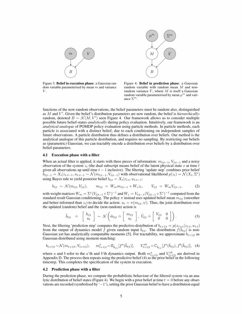
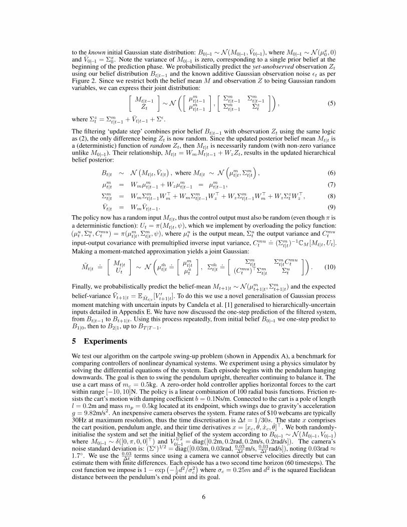
Here we describe the novel aspects of our method. Our method uses the same high-level algorithmas PILCO (Algorithm 1). However, we modify (using PILCO’s source code http://mlg.eng.cam.ac.uk/pilco/) two subroutines to extend PILCO from MDPs to a special-case of POMDPs(specifically where the partial observability has the form of additive Gaussian noise on the unobservedstate X). First, we filter observations during system execution (Algorithm 1, line 4), detailed inSection 4.1. Second, we predict belief -trajectories instead of state-trajectories (line 6), detailedsection 4.2. Filtering maintains a belief posterior of the latent system state. The belief is conditionedon, not just the most recent observation, but all previous observations (Figure 2). Such additionalconditioning has the benefit of providing a less-noisy and more-informed input to the policy: thefiltered belief-mean instead of the raw observation zt. Our implementation continues PILCO’sdistinction between executing the system (resulting in a single real belief-trajectory) and predictingthe system’s responses (which in our case yields an analytic distribution of multiple possible futurebelief-trajectories). During the execution phase, the system reads specific observations zt. Ourmethod additionally maintains a belief state b ∼ N (m,V ) by filtering observations. This beliefstate b can be treated as a random variable with a distribution parameterised by belief-mean m andbelief-certainty V seen Figure 3. Note both m and V are functions of previous observations z1:t.Now, during the (probabilistic) prediction phase, future observations are instead random variables(since they have not been observed yet), distinguished as Z. Since the belief parameters m and V are
Xt Xt+1
Zt Ut Zt+1π
f
Figure 1: The original (unfiltered) PILCO,as a probabilistic graphical model. At eachtimestep, the latent system Xt is observed nois-ily as Zt which is inputted directly into policyfunction π to decide action Ut. Finally, the la-tent system will evolve to Xt+1, according tothe unknown, nonlinear dynamics function fof the previous state Xt and action Ut.
Bt|t−1 Bt|t Bt+1|t
Zt Ut Zt+1
π
f
Figure 2: Our method (PILCO extended with Bayesianfiltering). Our prior belief Bt|t−1 (over latent systemXt), generates observation Zt. The prior belief Bt|t−1
then combines with observation Zt resulting in posteriorbelief Bt|t (the update step). Then, the mean posteriorbelief E[Bt|t] is inputted into policy function π to decideaction Ut. Finally, the next timestep’s prior belief Bt+1|tis predicted using dynamics model f (the prediction step).
4
m V
B
Figure 3: Belief in execution phase: a Gaussian ran-dom variable parameterised by mean m and varianceV .
µm Σm
M V
B
Figure 4: Belief in prediction phase: a Gaussianrandom variable with random mean M and non-random variance V , where M is itself a Gaussianrandom variable parameterised by mean µm and vari-ance Σm.
functions of the now-random observations, the belief parameters must be random also, distinguishedas M and V ′. Given the belief’s distribution parameters are now random, the belief is hierarchically-random, denoted B ∼ N (M,V ′) seen Figure 4. Our framework allows us to consider multiplepossible future belief-states analytically during policy evaluation. Intuitively, our framework is ananalytical analogue of POMDP policy evaluation using particle methods. In particle methods, eachparticle is associated with a distinct belief, due to each conditioning on independent samples offuture observations. A particle distribution thus defines a distribution over beliefs. Our method is theanalytical analogue of this particle distribution, and requires no sampling. By restricting our beliefsas (parametric) Gaussian, we can tractably encode a distribution over beliefs by a distribution overbelief-parameters.
4.1 Execution phase with a filterWhen an actual filter is applied, it starts with three pieces of information: mt|t−1, Vt|t−1 and a noisyobservation of the system zt (the dual subscript means belief of the latent physical state x at time tgiven all observations up until time t− 1 inclusive). The filtering ‘update step’ combines prior beliefbt|t−1 = Xt|z1:t−1, u1:t−1 ∼ N (mt|t−1, Vt|t−1) with observational likelihood p(zt) = N (Xt,Σ
ε)using Bayes rule to yield posterior belief bt|t = Xt|z1:t, u1:t−1:
bt|t ∼ N (mt|t, Vt|t), mt|t = Wmmt|t−1 +Wzzt, Vt|t = WmVt|t−1, (2)
with weight matricesWm = Σε(Vt|t−1+Σε)−1 andWz = Vt|t−1(Vt|t−1+Σε)−1 computed from thestandard result Gaussian conditioning. The policy π instead uses updated belief-mean mt|t (smootherand better-informed than zt) to decide the action: ut = π(mt|t, ψ). Thus, the joint distribution overthe updated (random) belief and the (non-random) action is
bt|t.=
[bt|tut
]∼ N
(mt|t
.=
[mt|tut
], Vt|t
.=
[Vt|t 00 0
]). (3)
Next, the filtering ‘prediction step’ computes the predictive-distribution of bt+1|t = p(xt+1|z1:t, u1:t)from the output of dynamics model f given random input bt|t. The distribution f(bt|t) is non-Gaussian yet has analytically computable moments [5]. For tractability, we approximate bt+1|t asGaussian-distributed using moment-matching:
bt+1|t∼N (mt+1|t, Vt+1|t), mat+1|t=Ebt|t [f
a(bt|t)], V abt+1|t=Cbt|t [fa(bt|t), f
b(bt|t)], (4)
where a and b refer to the a’th and b’th dynamics output. Both mat+1|t and V abt+1|t are derived in
Appendix D. The process then repeats using the predictive belief (4) as the prior belief in the followingtimestep. This completes the specification of the system in execution.
4.2 Prediction phase with a filterDuring the prediction phase, we compute the probabilistic behaviour of the filtered system via an ana-lytic distribution of belief states (Figure 4). We begin with a prior belief at time t = 0 before any obser-vations are recorded (symbolised by ‘−1’), setting the prior Gaussian belief to have a distribution equal
5
to the known initial Gaussian state distribution: B0|−1 ∼ N (M0|−1, V0|−1), where M0|−1 ∼ N (µx0 , 0)and V0|−1 = Σx0 . Note the variance of M0|−1 is zero, corresponding to a single prior belief at thebeginning of the prediction phase. We probabilistically predict the yet-unobserved observation Ztusing our belief distribution Bt|t−1 and the known additive Gaussian observation noise εt as perFigure 2. Since we restrict both the belief mean M and observation Z to being Gaussian randomvariables, we can express their joint distribution:[
Mt|t−1
Zt
]∼ N
([µmt|t−1
µmt|t−1
],
[Σmt|t−1 Σmt|t−1
Σmt|t−1 Σzt
]), (5)
where Σzt = Σmt|t−1 + Vt|t−1 + Σε.
The filtering ‘update step’ combines prior belief Bt|t−1 with observation Zt using the same logicas (2), the only difference being Zt is now random. Since the updated posterior belief mean Mt|t isa (deterministic) function of random Zt, then Mt|t is necessarily random (with non-zero varianceunlike M0|−1). Their relationship, Mt|t = WmMt|t−1 +WzZt, results in the updated hierarchicalbelief posterior:
Bt|t ∼ N(Mt|t, Vt|t
), where Mt|t ∼ N
(µmt|t,Σ
mt|t
), (6)
µmt|t = Wmµmt|t−1 +Wzµ
mt|t−1 = µmt|t−1, (7)
Σmt|t = WmΣmt|t−1W>m +WmΣmt|t−1W
>z +WzΣ
mt|t−1W
>m +WzΣ
ztW>z , (8)
Vt|t = WmVt|t−1. (9)
The policy now has a random inputMt|t, thus the control output must also be random (even though π isa deterministic function): Ut = π(Mt|t, ψ), which we implement by overloading the policy function:(µut ,Σ
ut , C
mut ) = π(µmt|t,Σ
mt|t, ψ), where µut is the output mean, Σut the output variance and Cmut
input-output covariance with premultiplied inverse input variance, Cmut.= (Σmt|t)
−1CM [Mt|t, Ut].Making a moment-matched approximation yields a joint Gaussian:
Mt|t.=
[Mt|tUt
]∼ N
(µmt|t
.=
[µmt|tµut
], Σmt|t
.=
[Σmt|t Σmt|tC
mut
(Cmut )>Σmt|t Σut
]). (10)
Finally, we probabilistically predict the belief-mean Mt+1|t ∼ N (µmt+1|t,Σmt+1|t) and the expected
belief-variance Vt+1|t = EMt|t[V ′t+1|t]. To do this we use a novel generalisation of Gaussian process
moment matching with uncertain inputs by Candela et al. [1] generalised to hierarchically-uncertaininputs detailed in Appendix E. We have now discussed the one-step prediction of the filtered system,from Bt|t−1 to Bt+1|t. Using this process repeatedly, from initial belief B0|−1 we one-step predict toB1|0, then to B2|1, up to BT |T−1.
5 Experiments
We test our algorithm on the cartpole swing-up problem (shown in Appendix A), a benchmark forcomparing controllers of nonlinear dynamical systems. We experiment using a physics simulator bysolving the differential equations of the system. Each episode begins with the pendulum hangingdownwards. The goal is then to swing the pendulum upright, thereafter continuing to balance it. Theuse a cart mass of mc = 0.5kg. A zero-order hold controller applies horizontal forces to the cartwithin range [−10, 10]N. The policy is a linear combination of 100 radial basis functions. Friction re-sists the cart’s motion with damping coefficient b = 0.1Ns/m. Connected to the cart is a pole of lengthl = 0.2m and mass mp = 0.5kg located at its endpoint, which swings due to gravity’s accelerationg = 9.82m/s2. An inexpensive camera observes the system. Frame rates of $10 webcams are typically30Hz at maximum resolution, thus the time discretisation is ∆t = 1/30s. The state x comprisesthe cart position, pendulum angle, and their time derivatives x = [xc, θ, xc, θ]
>. We both randomly-initialise the system and set the initial belief of the system according to B0|−1 ∼ N (M0|−1, V0|−1)where M0|−1 ∼ δ([0, π, 0, 0]>) and V
1/20|−1 = diag([0.2m, 0.2rad, 0.2m/s, 0.2rad/s]). The camera’s
noise standard deviation is: (Σε)1/2 = diag([0.03m, 0.03rad, 0.03∆t m/s, 0.03
∆t rad/s]), noting 0.03rad ≈1.7◦. We use the 0.03
∆t terms since using a camera we cannot observe velocities directly but canestimate them with finite differences. Each episode has a two second time horizon (60 timesteps). Thecost function we impose is 1− exp
(− 1
2d2/σ2
c
)where σc = 0.25m and d2 is the squared Euclidean
distance between the pendulum’s end point and its goal.
6
We compare four algorithms: 1) PILCO by Deisenroth and Rasmussen [5] as a baseline (unfilteredexecution, and unfiltered full-prediction); 2) the method by Dallaire et al. [3] (filtered execution,and filtered MAP-prediction); 3) the method by Deisenroth and Peters [4] (filtered execution, andunfiltered full-prediction); and lastly 4) our method (filtered execution, and filtered full-prediction).For clear comparison we first control for data and dynamics models, where each algorithm has accessto the exact same data and exact same dynamics model. The reason is to eliminate variance inperformance caused by different algorithms choosing different actions. We generate a single datasetby running the baseline PILCO algorithm for 11 episodes (totalling 22 seconds of system interaction).The independent variables of our first experiment are 1) the method of system prediction and 2) themethod of system execution. Each policy is then optimised from the same initialisation using theirrespective prediction methods, before comparing performances. Afterwards, we experiment allowingeach algorithm to collect its own data, and also experiment with various noise level.
6 Results and analysis
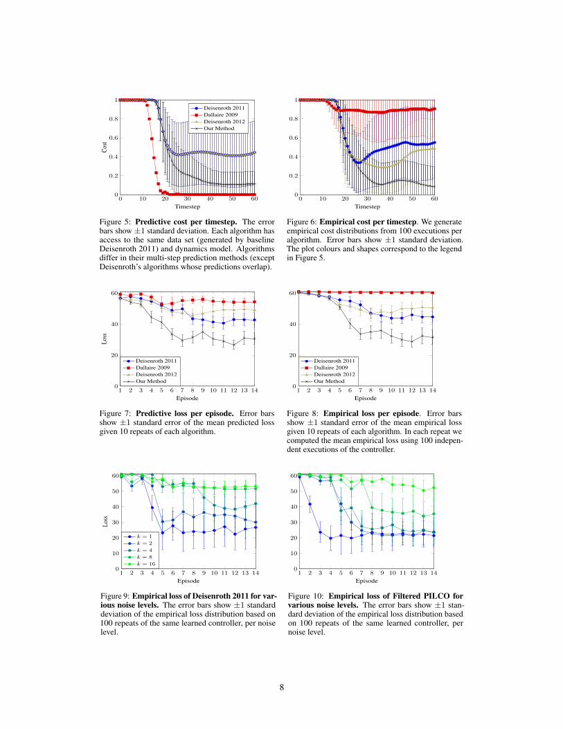
6.1 Results using a common datasetWe now compare algorithm performance, both predictive (Figure 5) and empirical (Figure 6). First,we analyse predictive costs per timestep (Figure 5). Since predictions are probabilistic, the costshave distributions, with the exception of Dallaire et al. [3] which predicts MAP trajectories andtherefore has deterministic cost. Even though we plot distributed costs, policies are optimised w.r.t.expected total cost only. Using the same dynamics, the different prediction methods optimise differentpolicies (with the exception of Deisenroth and Rasmussen [5] and Deisenroth and Peters [4], whoseprediction methods are identical). During the first 10 timesteps, we note identical performance withmaximum cost due to the non-zero time required to physically swing the pendulum up near the goal.Performances thereafter diverge. Since we predict w.r.t. a filtering process, less noise is predicted tobe injected into the policy, and the optimiser can thus afford higher gain parameters w.r.t. the pole atbalance point. If we linearise our policy around the goal point, our policy has a gain of -81.7N/radw.r.t. pendulum angle, a larger-magnitude than both Deisenroth method gains of -39.1N/rad (negativevalues refer to left forces in Figure 11). This higher gain is advantageous here, corresponding to amore reactive system which is more likely to catch a falling pendulum. Finally, we note Dallaire et al.[3] predict very high performance. Without balancing the costs across multiple possible trajectories,the method instead optimises a sequence of deterministic states to near perfection.
To compare the predictive results against the empirical, we used 100 executions of each algorithm(Figure 6). First, we notice a stark difference between predictive and executed performances fromDallaire et al. [3], due to neglecting model uncertainty, suffering model bias. In contrast, the othermethods consider uncertainty and have relatively unbiased predictions, judging by the similaritybetween predictive-vs-empirical performances. Deisenroth’s methods, which differ only in execution,illustrate that filtering during execution-only can be better than no filtering at all. However, the majorbenefit comes when the policy is evaluated from multi-step predictions of a filtered system. Opposedto Deisenroth and Peters [4], our method’s predictions reflect reality closer because we both predictand execute system trajectories using closed loop filtering control.
To test statistical significance of empirical cost differences given 100 executions, we use a Wilcoxonrank-sum test at each time step. Excluding time steps ranging t = [0, 29] (whose costs are similar),the minimum z-score over timesteps t = [30, 60] that our method has superior average-cost than eachother methods follows: Deisenroth 2011 min(z) = 4.99, Dallaire 2009’s min(z) = 8.08, Deisenroth2012’s min(z) = 3.51. Since the minimum min(z) = 3.51, we have p > 99.9% certainty ourmethod’s average empirical cost is superior than each other method.
6.2 Results of full reinforcement learning taskIn the previous experiment we used a common dataset to compare each algorithm, to isolate and focuson how well each algorithm makes use of data, rather than also considering the different ways eachalgorithm collects different data. Here, we remove the constraint of a common dataset, and test thefull reinforcement learning task by allowing each algorithm to collect its own data over repeated trialsof the cart-pole task. Each algorithm is allowed 15 trials (episodes), repeated 10 times with differentrandom seeds. For a particular re-run experiment and episode number, an algorithm’s predicted lossis unchanged when repeatedly computed, yet the empirical loss differs due to random initial states,observation noise, and process noise. We therefore average the empirical results over 100 randomexecutions of the controller at each episode and seed.
7
0 10 20 30 40 50 600
0.2
0.4
0.6
0.8
1
Timestep
Cost
Deisenroth 2011Dallaire 2009Deisenroth 2012Our Method
Figure 5: Predictive cost per timestep. The errorbars show ±1 standard deviation. Each algorithm hasaccess to the same data set (generated by baselineDeisenroth 2011) and dynamics model. Algorithmsdiffer in their multi-step prediction methods (exceptDeisenroth’s algorithms whose predictions overlap).
0 10 20 30 40 50 600
0.2
0.4
0.6
0.8
1
Timestep
Figure 6: Empirical cost per timestep. We generateempirical cost distributions from 100 executions peralgorithm. Error bars show ±1 standard deviation.The plot colours and shapes correspond to the legendin Figure 5.
1 2 3 4 5 6 7 8 9 10 11 12 13 140
20
40
60
Episode
Loss
Deisenroth 2011Dallaire 2009Deisenroth 2012Our Method
Figure 7: Predictive loss per episode. Error barsshow ±1 standard error of the mean predicted lossgiven 10 repeats of each algorithm.
1 2 3 4 5 6 7 8 9 10 11 12 13 140
20
40
60
Episode
Deisenroth 2011Dallaire 2009Deisenroth 2012Our Method
Figure 8: Empirical loss per episode. Error barsshow ±1 standard error of the mean empirical lossgiven 10 repeats of each algorithm. In each repeat wecomputed the mean empirical loss using 100 indepen-dent executions of the controller.
1 2 3 4 5 6 7 8 9 10 11 12 13 140
10
20
30
40
50
60
Episode
Loss
k = 1
k = 2
k = 4
k = 8
k = 16
Figure 9: Empirical loss of Deisenroth 2011 for var-ious noise levels. The error bars show ±1 standarddeviation of the empirical loss distribution based on100 repeats of the same learned controller, per noiselevel.
1 2 3 4 5 6 7 8 9 10 11 12 13 140
10
20
30
40
50
60
Episode
Figure 10: Empirical loss of Filtered PILCO forvarious noise levels. The error bars show ±1 stan-dard deviation of the empirical loss distribution basedon 100 repeats of the same learned controller, pernoise level.
8
The predictive loss (cumulative cost) distributions of each algorithm are shown Figure 7. Perhapsthe most striking difference between the full reinforcement learning predictions and those madewith a controlled dataset (Figure 5) is that Dallaire does not predict it will perform well. Thequality of the data collected by Dallaire within the first 15 episodes is not sufficient to predictgood performance. Our Filtered PILCO method accurately predicts its own strong performance andadditionally outperforms the competing algorithm seen in Figure 8. Of interest is how each algorithmperforms equally poorly during the first four episodes, with Filtered PILCO’s performance breakingaway and learning the task well by the seventh trial. Such a learning rate was similar to the originalPILCO experiment with the noise-free cartpole.
6.3 Results with various observation noisesDifferent observation noise levels were also tested, comparing PILCO (Figure 9) with FilteredPILCO (Figure 10). Both figures show a noise factors k, such that the observation noise is:√
Σε=k × diag([0.01m, 0.01rad, 0.01∆t m/s, 0.01
∆t rad/s]). For reference, our previous experiments useda noise factor of k = 3. At low noise factor k = 1, both algorithms perform similarly-well, sinceobservations are precise enough to control a system without a filter. As observations noise increases,the performance of unfiltered PILCO soon drops, whilst the Filtered PILCO can successfully controlthe system under higher noise levels (Figure 10).
6.4 Training time complexityTraining the GP dynamics model involved N = 660 data points, M = 50 inducing points undera sparse GP Fully Independent Training Conditional (FITC) [2], P = 100 policy RBF centroids,D = 4 state dimensions, F = 1 action dimensions, and T = 60 timestep horizon, with timecomplexity O(DNM2). Policy optimisation (with 300 steps, each of which require trajectoryprediction with gradients) is the most intense part: our method and both Deisenroth’s methods scaleO(M2D2(D + F )2T + P 2D2F 2T ), whilst Dallaire’s only scales O(MD(D + F )T + PDFT ).Worst case we require M = O(exp(D + F )) inducing points to capture dynamics, the average caseis unknown. Total training time was four hours to train the original PILCO method with an additionalone hour to re-optimise the policy.
7 Conclusion and future work
In this paper, we extended the original PILCO algorithm [5] to filter observations, both during systemexecution and multi-step probabilistic prediction required for policy evaluation. The extended frame-work enables learning in a special case of partially-observed MDP environments (POMDPs) whilstretaining PILCO’s data-efficiency property. We demonstrated successful application to a benchmarkcontrol problem, the noisily-observed cartpole swing-up. Our algorithm learned a good policy undersignificant observation noise in less than 30 seconds of system interaction. Importantly, our algorithmevaluates policies with predictions that are faithful to reality: we predict w.r.t. closed loop filteredcontrol precisely because we execute closed loop filtered control. We showed experimentally thatfaithful and probabilistic predictions improved performance with respect to the baselines. For clearcomparison we first constrained each algorithm to use the same dynamics dataset to demonstrate su-perior data-usage of our algorithm. Afterwards we relaxed this constraint, and showed our algorithmwas able to learn from fewer data.
Several more challenges remain for future work. Firstly the assumption of zero variance of thebelief-variance could be relaxed. A relaxation allows distributed trajectories to more accuratelyconsider belief states having various degrees of certainty (belief-variance). For example, systemtrajectories have larger belief-variance when passing though data-sparse regions of state-space, andsmaller belief-variance in data-dense regions. Secondly, the policy could be a function of the fullbelief distribution (mean and variance) rather than just the mean. Such flexibility could help the policymake more ‘cautious’ actions when more uncertain about the state. A third challenge is handlingnon-Gaussian noise and unobserved state variables. For example, in real-life scenarios using a camerasensor for self-driving, observations are occasionally fully or partially occluded, or limited by weatherconditions, where such occlusions and limitations change, opposed to assuming a fixed Gaussianaddition noise. Lastly, experiments with a real robot would be important to show the usefulness inpractice.
9
References
[1] Joaquin Candela, Agathe Girard, Jan Larsen, and Carl Rasmussen. Propagation of uncertainty in Bayesiankernel models-application to multiple-step ahead forecasting. In International Conference on Acoustics,Speech, and Signal Processing, volume 2, pages 701–704, 2003.
[2] Lehel Csató and Manfred Opper. Sparse on-line Gaussian processes. Neural Computation, 14(3):641–668,2002.
[3] Patrick Dallaire, Camille Besse, Stephane Ross, and Brahim Chaib-draa. Bayesian reinforcement learningin continuous POMDPs with Gaussian processes. In International Conference on Intelligent Robots andSystems, pages 2604–2609, 2009.
[4] Marc Deisenroth and Jan Peters. Solving nonlinear continuous state-action-observation POMDPs formechanical systems with Gaussian noise. In European Workshop on Reinforcement Learning, 2012.
[5] Marc Deisenroth and Carl Rasmussen. PILCO: A model-based and data-efficient approach to policy search.In International Conference on Machine Learning, pages 465–472, New York, NY, USA, 2011.
[6] Michael Duff. Optimal Learning: Computational procedures for Bayes-adaptive Markov decision pro-cesses. PhD thesis, Department of Computer Science, University of Massachusetts Amherst, 2002.
[7] Jonathan Ko and Dieter Fox. GP-BayesFilters: Bayesian filtering using Gaussian process prediction andobservation models. Autonomous Robots, 27(1):75–90, 2009.
[8] Timothy Lillicrap, Jonathan Hunt, Alexander Pritzel, Nicolas Heess, Tom Erez, Yuval Tassa, David Silver,and Daan Wierstra. Continuous control with deep reinforcement learning. In arXiv preprint, arXiv1509.02971, 2015.
[9] Andrew McHutchon. Nonlinear modelling and control using Gaussian processes. PhD thesis, Departmentof Engineering, University of Cambridge, 2014.
[10] Pascal Poupart, Nikos Vlassis, Jesse Hoey, and Kevin Regan. An analytic solution to discrete Bayesianreinforcement learning. International Conference on Machine learning, pages 697–704, 2006.
[11] Carl Rasmussen and Chris Williams. Gaussian Processes for Machine Learning. MIT Press, Cambridge,MA, USA, 1 2006.
[12] Stephane Ross, Brahim Chaib-draa, and Joelle Pineau. Bayesian reinforcement learning in continuousPOMDPs with application to robot navigation. In International Conference on Robotics and Automation,pages 2845–2851, 2008.
[13] Jur van den Berg, Sachin Patil, and Ron Alterovitz. Efficient approximate value iteration for continuousGaussian POMDPs. In Association for the Advancement of Artificial Intelligence, 2012.
[14] Dustin Webb, Kyle Crandall, and Jur van den Berg. Online parameter estimation via real-time replanning ofcontinuous Gaussian POMDPs. In International Conference Robotics and Automation, pages 5998–6005,2014.
10
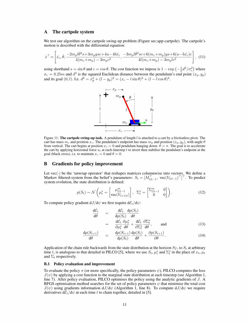
A The cartpole system
We test our algorithm on the cartpole swing-up problem (Figure sec:app-cartpole). The cartpole’smotion is described with the differential equation:
x>=
[xc, θ,
−2mplθ2s+3mpgsc+4u−4bxc
4(mc+mp)− 3mpc2,−3mplθ
2sc+6(mc+mp)gs+6(u−bxc)c4l(mc+mp)− 3mplc2
], (11)
using shorthand s = sin θ and c = cos θ. The cost function we impose is 1− exp(− 1
2d2/σ2
c
)where
σc = 0.25m and d2 is the squared Euclidean distance between the pendulum’s end point (xp, yp)and its goal (0, l). I.e. d2 = x2
p + (l − yp)2 = (xc − l sin θ)2 + (l − l cos θ)2.
mc
mp
l
θ
xc
yp
xp
l
u
Figure 11: The cartpole swing-up task. A pendulum of length l is attached to a cart by a frictionless pivot. Thecart has mass mc and position xc. The pendulum’s endpoint has mass mp and position (xp, yp), with angle θfrom vertical. The cart begins at position xc = 0 and pendulum hanging down: θ = π. The goal is to acceleratethe cart by applying horizontal force ut at each timestep t to invert then stabilise the pendulum’s endpoint at thegoal (black cross), i.e. to maintain xc = 0 and θ = 0.
B Gradients for policy improvement
Let vec(·) be the ‘unwrap operator’ that reshapes matrices columnwise into vectors. We define aMarkov filtered-system from the belief’s parameters: St = [M>t|t−1, vec(Vt|t−1)>]>. To predictsystem evolution, the state distribution is defined:
p(St) ∼ N(µst =
[µmt|t−1
vec(Vt+1|t)
], Σst =
[Σmt|t−1 0
0 0
]). (12)
To compute policy gradient dJ/dψ we first require dEt/dψ:
dEtdθ
=dEt
dp(St)dp(St)
dθ
=dEt∂µst
∂µstdθ
+dEt∂Σst
∂Σstdθ
, and (13)
dp(St+1)
dθ=
dp(St+1)
dp(St)dp(St)
dθ+∂p(St+1)
∂θ. (14)
Application of the chain rule backwards from the state distribution at the horizon ST , to St at arbitrarytime t, is analogous to that detailed in PILCO [5], where we use St, µst and Σst in the place of xt, µtand Σt respectively.
B.1 Policy evaluation and improvementTo evaluate the policy π (or more specifically, the policy parameters ψ), PILCO computes the lossJ(ψ) by applying a cost function to the marginal state distribution at each timestep (see Algorithm 1,line 7). After policy evaluation, PILCO optimises the policy using the analytic gradients of J . ABFGS optimisation method searches for the set of policy parameters ψ that minimise the total costJ(ψ) using gradients information dJ/dψ (Algorithm 1, line 8). To compute dJ/dψ we requirederivatives dEt/dψ at each time t to chain together, detailed in [5].
11
B.2 Policy evaluation and improvement with a filterTo evaluate a policy we again apply the loss function J (Algorithm 1, line 7) to the multi-stepprediction (section 4.2). The policy is again optimised using the analytic gradients of J . SinceJ now is a function of beliefs, we additionally consider the gradients of Bt|t−1 w.r.t. ψ. As thebelief is distributed byBt|t−1 ∼ N (Mt|t−1, Vt|t−1) ∼ N (N (µmt|t−1,Σ
mt|t−1), Vt|t−1), we use partial
derivatives of µmt|t−1, Σmt|t−1 and Vt|t−1 w.r.t. each other and w.r.t ψ.
C Identities for Gaussian process prediction with hierarchical uncertain in-puts
The two functions
q(x, x′,Λ, V ) , |Λ−1V + I|−1/2 exp(− 1
2 (x− x′)[Λ + V ]−1(x− x′)),
Q(x, x′,Λa,Λb, V, µ,Σ) , c1 exp(− 1
2 (x− x′)>[Λa + Λb + 2V ]−1(x− x′))
× exp(− 1
2 (z − µ)>[(
(Λa + V )−1 + (Λb + V )−1)−1
+ Σ]−1
(z − µ)),
= c2 q(x, µ,Λa, V ) q(µ, x′Λb, V )
× exp(
12r>[(Λa + V )−1 + (Λb + V )−1 + Σ−1
]−1r),
where
z = (Λb + V )(Λa + Λb + 2V )−1x+ (Λa + V )(Λa + Λb + 2V )−1x′
r = (Λa + V )−1(x− µ) + (Λb + V )−1(x′ − µ)
c1 =∣∣(Λa + V )(Λb + V ) + (Λa + Λb + 2V )Σ
∣∣−1/2∣∣ΛaΛb∣∣1/2
c2 =∣∣((Λa + V )−1 + (Λb + V )−1
)Σ + I
∣∣−1/2,
(15)
have the following Gaussian integrals∫q(x, t,Λ, V )N (t|µ,Σ)dt = q(x, µ,Λ,Σ + V ),∫
q(x, t,Λa, V ) q(t, x′,Λb, V )N (t|µ,Σ)dt = Q(x, x′,Λa,Λb, V, µ,Σ),∫Q(x, x′,Λa,Λb, 0, µ, V )N (µ|m,Σ)dµ = Q(x, x′,Λa,Λb, 0,m,Σ + V ).
(16)
We want to model data with E output coordinates, and use separate combinations of linear modelsand GPs to make predictions, a = 1, . . . , E:
fa(x∗) = f∗a ∼ N(θ>a x
∗ + ka(x∗,x)βa, ka(x∗, x∗)− ka(x∗,x)(Ka + Σaε)−1ka(x, x∗)),
where the E squared exponential covariance functions are
ka(x, x′) = s2aq(x, x
′,Λa, 0), where a = 1, . . . , E, (17)
and s2a are the signal variances and Λa is a diagonal matrix of squared length scales for GP number
a. The noise variances are Σaε . The inputs are x and the outputs ya and we define βa = (Ka +Σaε)−1(ya − θ>a x), where Ka is the Gram matrix.
C.1 DerivativesFor symmetric Λ and V and Σ:
∂ ln q(x, x′,Λ, V )
∂x= − (Λ + V )−1(x− x′) = −(Λ−1V + I)−1Λ−1(x− x′)
∂ ln q(x, x′,Λ, V )
∂x′= (Λ + V )−1(x− x′)
∂ ln q(x, x′,Λ, V )
∂V= − 1
2(Λ + V )−1 +
1
2(Λ + V )−1(x− x′)(x− x′)>(Λ + V )−1
(18)
12
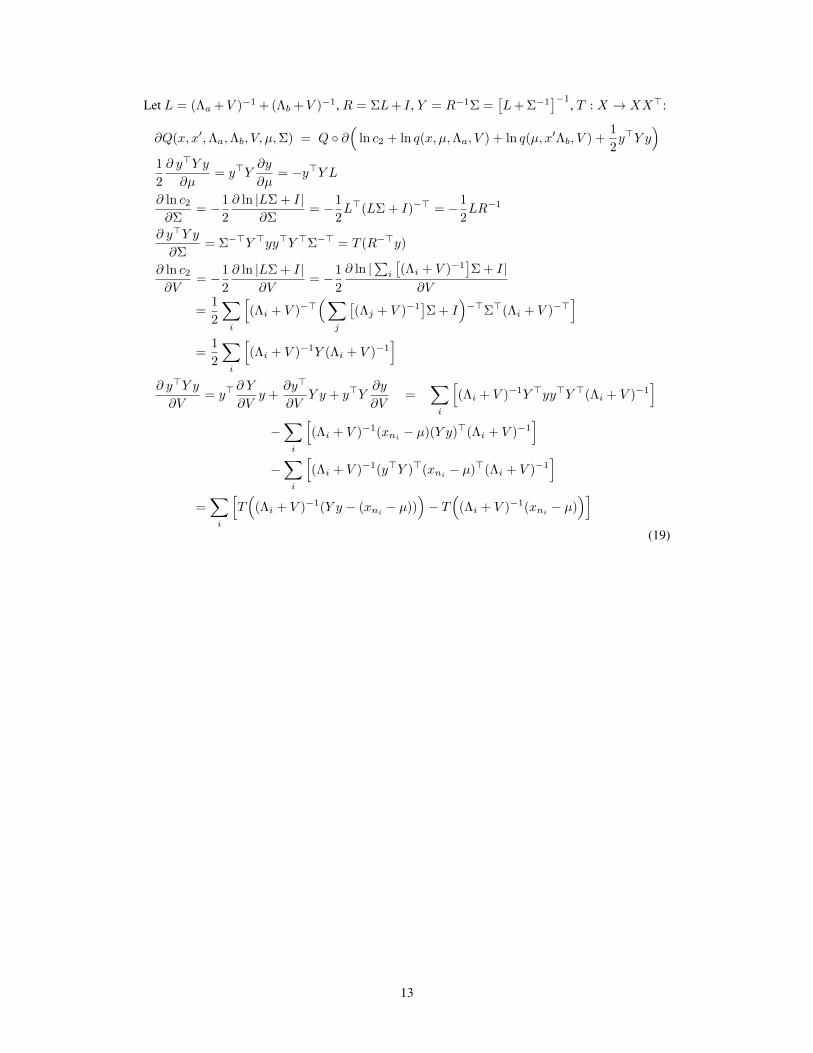
Let L = (Λa +V )−1 + (Λb +V )−1, R = ΣL+ I , Y = R−1Σ =[L+ Σ−1
]−1, T : X → XX>:
∂Q(x, x′,Λa,Λb, V, µ,Σ) = Q ◦ ∂(
ln c2 + ln q(x, µ,Λa, V ) + ln q(µ, x′Λb, V ) +1
2y>Y y
)1
2
∂ y>Y y
∂µ= y>Y
∂y
∂µ= −y>Y L
∂ ln c2∂Σ
= −1
2
∂ ln |LΣ + I|∂Σ
= −1
2L>(LΣ + I)−> = −1
2LR−1
∂ y>Y y
∂Σ= Σ−>Y >yy>Y >Σ−> = T (R−>y)
∂ ln c2∂V
= −1
2
∂ ln |LΣ + I|∂V
= −1
2
∂ ln |∑i
[(Λi + V )−1
]Σ + I|
∂V
=1
2
∑i
[(Λi + V )−>
(∑j
[(Λj + V )−1
]Σ + I
)−>Σ>(Λi + V )−>
]=
1
2
∑i
[(Λi + V )−1Y (Λi + V )−1
]∂ y>Y y
∂V= y>
∂ Y
∂Vy +
∂y>
∂VY y + y>Y
∂y
∂V=
∑i
[(Λi + V )−1Y >yy>Y >(Λi + V )−1
]−∑i
[(Λi + V )−1(xni − µ)(Y y)>(Λi + V )−1
]−∑i
[(Λi + V )−1(y>Y )>(xni − µ)>(Λi + V )−1
]=∑i
[T(
(Λi + V )−1(Y y − (xni − µ)))− T
((Λi + V )−1(xni − µ)
)](19)
13
D Dynamics predictions in execution phase
Here we specify the predictive distribution p(bt+1|t), whose moments are equal to the momentsfrom dynamics model output f with uncertain input bt|t ∼ N (mt|t, Vt|t) similar to Deisenroth andRasmussen [5] which was based on work by Candela et al. [1]. Consider making predictions froma = 1, . . . , E GPs at bt|t with specification bt|t ∼ N (mt|t, Vt|t). We have the following expressionsfor the predictive mean, variances and input-output covariances using the law of iterated expectationsand variances:
bt+1|t ∼ N (mt+1|t, Vt+1|t), (20)
mat+1|t = Ebt|t [f
a(bt|t)]
=
∫ (s2aβ>a q(xi, bt|t,Λa, 0) + φ>a bt|t
)N (bt|t; mt|t, Vt|t)dbt|t
= s2aβ>a q
a + φ>a mt|t, (21)
Ca.= V −1
t|t Cbt|t [bt|t, fa(bt|t)− φ>a bt|t],
= V −1t|t
∫(bt|t − mt|t)s
2aβ>a q(x, bt|t,Λa, 0)N (bt|t; mt|t, Vt|t)dbt|t
= s2a(Λa + Vt|t)
−1(x− mt|t)βaqa, (22)
V abt+1|t = Cbt|t[fa(bt|t), f
b(bt|t)]
= Cbt|t[Ef [fa(bt|t),Ef [f b(bt|t)
]+ Ebt|t
[Cf [fa(bt|t), f
b(bt|t)]]
= Cbt|t[s2aβ>a q(x, bt|t,Λa, 0) + φ>a bt|t, s2
bβ>b q(x, bt|t,Λb, 0) + φ>b bt|t
]+
δabE[s2a − ka(bt|t, x)(Ka + Σaε)−1ka(x, bt|t)]
= s2as
2b
[β>a (Qab−qaqb>)βb +
δab(s−2a −tr((Ka + Σaε)−1Qaa)
)]+ C>a Vt|tφb + φ>a Vt|tCb + φ>a Vt|tφb, (23)
where
qai = q(xi, mt|t,Λa, Vt|t
),
Qabij = Q(xi, xj ,Λa,Λb, 0, mt|t, Vt|t
),
βa = (Ka + Σε,a)−1(ya − φ>a x),
and training inputs are x, outputs are ya (determined by the ‘Direct method’), Ka is a Gram matrix.
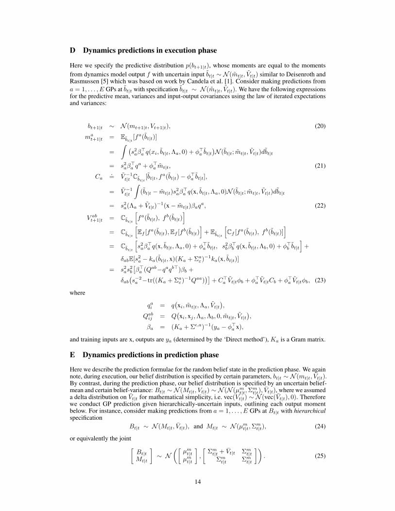
E Dynamics predictions in prediction phase
Here we describe the prediction formulae for the random belief state in the prediction phase. We againnote, during execution, our belief distribution is specified by certain parameters, bt|t ∼ N (mt|t, Vt|t).By contrast, during the prediction phase, our belief distribution is specified by an uncertain belief-mean and certain belief-variance: Bt|t ∼ N (Mt|t, Vt|t) ∼ N (N (µmt|t,Σ
mt|t), Vt|t), where we assumed
a delta distribution on Vt|t for mathematical simplicity, i.e. vec(Vt|t) ∼ N (vec(Vt|t), 0). Thereforewe conduct GP prediction given hierarchically-uncertain inputs, outlining each output momentbelow. For instance, consider making predictions from a = 1, . . . , E GPs at Bt|t with hierarchicalspecification
Bt|t ∼ N (Mt|t, Vt|t), and Mt|t ∼ N (µmt|t,Σmt|t), (24)
or equivalently the joint[Bt|tMt|t
]∼ N
([µmt|tµmt|t
],
[Σmt|t + Vt|t Σmt|t
Σmt|t Σmt|t
]). (25)
14

Mean of the Belief-Mean: dynamics prediction uses input Mt|t ∼ N (µmt|t,Σmt|t), which is jointly
distributed according to (10). Using the belief-mean mat+1|t definition (21),
µm,at+1|t = EMt|t[Ma
t+1|t]
=
∫Mat+1|tN (Mt|t;µ
mt|t,Σ
mt|t)dMt|t,
= s2aβ>a
∫q(x, Mt|t,Λa, Vt|t)N (Mt|t;µ
mt|t,Σ
mt|t)dMt|t + φ>a µ
mt|t
= s2aβ>a q
a + φ>a µmt|t, (26)
qai = q(xi, µ
mt|t,Λa,Σ
mt|t + Vt|t
). (27)
Input-Output Covariance: the expected input-output covariance belief term (22) (equivalent tothe input-output covariance of the belief-mean) is:
Ca.= V −1
t|t EMt|t[CBt|t [Bt|t, f(Bt|t)− φ>a Mt|t]], and similarly defined
.= (Σmt|t)
−1CMt|t[Mt|t,EBt|t [f(Bt|t)− φ>a Mt|t]],
= (Σmt|t)−1
∫(Mt|t − µmt|t)EBt|t [f(Bt|t)]N (Mt|t;µ
mt|t,Σ
mt|t)dMt|t
= (Σmt|t)−1
∫(Mt|t − µmt|t)
(s2aβ>a q(xi, Mt|t,Λa, Vt|t))N (Mt|t;µ
mt|t,Σ
mt|t)dMt|t
= s2a(Λa + Σmt|t + Vt|t)
−1(x− µmt|t)βaqai . (28)
Variance of the Belief-Mean: the variance of randomised belief-mean (Eq 21) is:
Σm,abt+1|t = CMt|t[Ma
t+1|t,Mbt+1|t],
=
∫Mat+1|tM
bt+1|tN (Mt|t|µmt|t,Σ
mt|t)dMt|t − µamt+1|t
µbmt+1|t,
= s2as
2bβ>a (Qab − qaqb>)βb + C>a Σmt|tφb + φ>a Σmt|tCb + φ>a Σmt|tφb, (29)
Qabij = Q(xi, xj ,Λa,Λb, Vt|t, µmt|t,Σmt|t). (30)
Mean of the Belief-Variance: using the belief-variance V abt+1|t definition (23),
V abt+1|t = EMt|t[V abt+1|t]
=
∫V abt+1|tN (Mt|t|µmt|t,Σ
mt|t)dMt|t
= s2as
2b
[β>a (Qab − Qab)βb + δab
(s−2a − tr((Ka + Σaε)−1Qaa)
)]+C>a Vt|tφb + φ>a Vt|tCb + φ>a Vt|tφb, (31)
Qabij = Q(xi, xj ,Λa,Λb, 0, µmt|t,Σmt|t + Vt|t). (32)
15