data efficient lithography modeling with residual neural...
TRANSCRIPT

Data Efficient Lithography Modeling with Residual NeuralNetworks and Transfer Learning
Yibo LinThe University of Texas at Austin
Yuki WatanabeToshiba Memory [email protected]
Taiki KimuraToshiba Memory [email protected]
Tetsuaki MatsunawaToshiba Memory Corporation
Shigeki NojimaToshiba Memory [email protected]
Meng LiThe University of Texas at Austin
David Z. PanThe University of Texas at Austin
ABSTRACTLithography simulation is one of the key steps in physical verification,enabled by the substantial optical and resist models. A resist modelbridges the aerial image simulation to printed patterns. While theeffectiveness of learning-based solutions for resist modeling has beendemonstrated, they are considerably data-demanding. Meanwhile, aset of manufactured data for a specific lithography configuration isonly valid for the training of one single model, indicating low dataefficiency. Due to the complexity of the manufacturing process, ob-taining enough data for acceptable accuracy becomes very expensivein terms of both time and cost, especially during the evolution of tech-nology generations when the design space is intensively explored. Inthis work, we propose a new resist modeling framework for contactlayers that utilizes existing data from old technology nodes to reducethe amount of data required from a target lithography configuration.Our framework based on residual neural networks and transfer learn-ing techniques is effective within a competitive range of accuracy,i.e., 2-10X reduction on the amount of training data with comparableaccuracy to the state-of-the-art learning approach.ACM Reference Format:Yibo Lin, Yuki Watanabe, Taiki Kimura, Tetsuaki Matsunawa, Shigeki Nojima,Meng Li, and David Z. Pan. 2018. Data Efficient Lithography Modeling withResidual Neural Networks and Transfer Learning . In Proceedings of 2018International Symposium on Physical Design (ISPD’18). ACM, New York, NY,USA, 8 pages. https://doi.org/10.1145/3177540.3178242
1 INTRODUCTIONDue to the continuous semiconductor scaling from 10nm technol-ogy node (N10) to 7nm node (N7) [10, 11], the prediction of printedpattern sizes is becoming increasingly difficult and complicated dueto the complexity of manufacturing process and variations. How-ever, complex designs demand accurate simulations to guaranteefunctionality and yield. Resist modeling, as a key component in
Permission to make digital or hard copies of all or part of this work for personal orclassroom use is granted without fee provided that copies are not made or distributedfor profit or commercial advantage and that copies bear this notice and the full citationon the first page. Copyrights for components of this work owned by others than ACMmust be honored. Abstracting with credit is permitted. To copy otherwise, or republish,to post on servers or to redistribute to lists, requires prior specific permission and/or afee. Request permissions from [email protected]’18, March 25–28, 2018, Monterey, CA, USA© 2018 Association for Computing Machinery.ACM ISBN 978-1-4503-5626-8/18/03. . . $15.00https://doi.org/10.1145/3177540.3178242
lithography simulation, is critical to bridge the aerial image simula-tion to manufactured wafer data. Rigorous simulations that performphysics-level modeling suffer from large computational overhead,which are not suitable when used extensively. Thus compact resistmodels are widely used in practice.
Figure 1(a) shows the process of lithography simulations wherethe optical model computes the aerial image from the input mask pat-terns and the resist model determines the output patterns from this.As the aerial image contains the light intensity map, the resist modelneeds to determine the slicing thresholds for the output patterns asshown in Figure 1(b). With the thresholds, the critical dimensions(CDs) of printed patterns can be computed, which need to matchCDs measured from manufactured patterns. In practice, various fac-tors may impact a resist model such as the physical properties ofphotoresist, design rules of patterns, process variations.
Accurate lithography simulation like rigorous physics-based sim-ulation is notorious for its long computational time, while simulationwith compact models suffers from accuracy issues [21, 25]. On theother hand, machine learning techniques are able to construct accu-rate models and then make efficient predictions. These approachesfirst take training data to calibrate a model and then use this modelto make predictions on testing data for validation. The effectivenessof learning-based solutions has been studied in various lithogra-phy related areas including aerial image simulation [15], hotspotdetection [13, 16, 22, 26, 28, 29], optical proximity correction (OPC)[5, 8, 14, 17], sub-resolution assist features (SRAF) [24, 27], resistmodeling [21, 25], etc. In resist modeling, a convolutional neuralnetwork (CNN) that predicts slicing thresholds in aerial images isproposed [25]. The neural network consists of three convolutionlayers and two fully connected layers. Since the slicing threshold is acontinuous value, learning a resist model is a regression task ratherthan a classification task. Around 70% improvement in accuracy isreported compared with calibrated compact models fromMentor Cal-ibre [18]. Shim et al. [21] propose an artificial neural network (ANN)with five hidden layers to predict the height of resist after exposure.Significant speedup is reported with high accuracy compared with arigorous simulation.
Although the learning-based approaches are able to achieve highaccuracy, they are generally data-demanding in model training. Inother words, big data is assumed to guarantee accuracy and gener-ality. Furthermore, one data sample can only be used to train the

Mask pattern Aerial image Resist pattern
Optical model Resist model
(a)
Slicingthreshold
Simulated CD
(b)Figure 1: (a) Process of lithography simulation with optical and re-sist models. (b) Thresholds for aerial image determine simulated CD,which should match manufactured CD.
corresponding model under the same lithography configuration, in-dicating a low data efficiency. Here data efficiency evaluates theaccuracy a model can achieve given a specific amount of data, orthe amount of data samples are required to achieve target accuracy.Nevertheless, obtaining a large amount of data is often expensive andtime-consuming, especially when the technology node switches fromone to another and the design space is under active exploration, e.g.,from N10 to N7. The lithography configurations including opticalsources, resist materials, etc., are frequently changed for experiments.Therefore, a fast preparation of models with high accuracy is urgentlydesired.
Different from previous approaches, in this work, we assume theavailability of large amounts of data from the previous technologygeneration with old lithography configurations and small amounts ofdata from a target lithography configuration. We focus on increasingthe data efficiency by reusing those from other lithography configu-rations and transfer the knowledge between different configurations.The objective is to achieve accurate resist models with significantlyfewer data to a target configuration. The major contributions aresummarized as follows.• We propose a high performance resist modeling techniquebased on the residual neural network (ResNet).• We propose a transfer learning scheme for ResNet that canreduce the amount of data with a target accuracy by utilizingthe data from other configurations.• We explore the impacts from various lithography configura-tions on the knowledge transfer.• The experimental results demonstrate 2-10X reduction in theamount of training data to achieve accuracy comparable tothe state-of-the-art learning approach [25].
The rest of the paper is organized as follows. Section 2 illustratesthe problem formulation. Section 3 explains the details of our ap-proach. The effectiveness of our approach is verified in Section 4 andthe conclusion is drawn in Section 5.
2 PRELIMINARIESIn this section, we will briefly introduce the background knowledgeon lithography simulation and resist modeling. Then the problemformulation is explained. We mainly focus on contact layers in thiswork, but our methodology shall be applicable to other layers.
2.1 Lithography SimulationLithography simulation is generally composed of two stages, i.e.,optical simulation and resist simulation, where optical and resistmodels are required, respectively. In the optical simulation, an opticalmodel, characterized by the illumination tool, takes mask patterns to
x
y
(a)
xy
Intensity
(b)
yc
(c)
x, y = yc
Intensity
(d)Figure 2: (a) Design target of 3 contacts and (b) the light intensityplot of aerial image. Assume that RETs such as SRAF and OPC havebeen already applied to the contacts before optical simulation. (c) Adotted line horizontally crosses the centers at y = yc and the circlesdenote the contours of printed patterns. (d) Light intensity profilingalong the dotted line at y = yc extracted from the aerial image anddifferent slicing thresholds for each contact.
compute aerial images, i.e., light intensity maps. Then in the resistsimulation, a resist model finalizes the resist patterns with the aerialimages from the optical simulation. Generally, there are two types ofresist models. One is a variable threshold resist (VTR) model in whichthe thresholds vary according to aerial images, and the other is aconstant threshold resist (CTR) model in which the light intensity ismodulated in an aerial image. We adopt the former since it is suitableto learning-based approaches [25].
Figure 2 shows an example of lithography simulation for a clipwith three contacts. We assume that proper resolution enhancementtechniques (RETs) such as OPC and SRAF have been applied beforethe computation of the aerial image [12]. The optical simulationgenerates the aerial image, as shown in Figure 2(b). Resist simulationthen computes the thresholds in the aerial image to predict printedpatterns. If we consider the horizontal sizes of contacts along thedotted line in Figure 2(c), the light intensity profiling can be extractedfrom the aerial image along the line and calculates the CDs for eachcontact with the thresholds.
2.2 Historical Data and Transfer LearningSince the lithography configurations evolve from one generation toanother with the advancement of technology nodes, there are plentyof historical data available for the old generation. As mentioned inSection 1, accurate models require a large amount of data for trainingor calibration, which are expensive to obtain during the explorationof a new generation. If the lithography configurations have no funda-mental changes, the knowledge learned from the historical data maystill be applicable to the new configuration, which can eventuallyhelp to reduce the amount of new data required.
Transfer learning represents a set of techniques to transfer theknowledge from one or multiple source domains to a target domain,utilizing the underlying similarity between the data from these do-mains. Various studies have explored the effectiveness of knowledgetransfer in image recognition and robotics [6, 19, 20], while it isnot clear whether the knowledge between different resist models istransferable or not.
In this work, we consider the evolution of the contact layer fromthe cutting edge technology node N10 to N7 [10, 11]. A large amount

Table 1: Lithography Configurations for N10 and N7
N10 N7N7a N7b
Design Rule A B B
Optical Source A B B
Resist Material A A B
(a) (b)Figure 3: Optical sources (yellow) for (a) N10 and (b) N7.
of available N10 data are assumed. During the evolution to N7, dif-ferent design rules for mask patterns, optical sources and resist ma-terials for lithography are explored. Table 1 shows the lithographyconfigurations considered for N10 and N7. Differences in letters A,Brepresent different configurations of design rules, optical sources, orresist materials. One configuration for N10 is considered, while twoconfigurations are considered for N7, i.e., N7a , N7b , with two kindsof resist materials (about 20% difference in the slopes of dissolutioncurves). From N10 to N7, both the design rules and optical sourcesare changed. For N10, we consider a pitch of 64nm with double pat-terning lithography, while for N7, the pitch is set to 45nm with triplepatterning lithography [10]. The width of each contact is set to halfpitch. The lithography target of each contact is set to 60nm for bothN10 and N7. Optical sources calibrated with industrial strength forN10 and N7 are shown in Figure 3, with the same type of illuminationshapes.
Various combinations of knowledge transfer can be explored fromTable 1, such as N10→N7, N7i→N7j , and N10+N7i→N7j , wherei , j, i, j ∈ {a,b}.
2.3 Learning-based Resist ModelingThe thresholds of positions near the contacts are of significant im-portance since they usually determine the boundaries of printedcontacts. Hence we consider the middle of the left, right, bottomand top edges for each contact, as shown in Figure 4(a), where thepositions for prediction are highlighted with black dots. In addition,the threshold is mainly influenced by the surrounding mask patterns.Therefore, resist models typically compute the threshold using aclip of mask patterns centered by a target position. To measure thethresholds in Figure 4(a), we select a clip where the target positionlies in its center, as shown in Figure 4(b) to Figure 4(e). The task of aresist model is to compute the thresholds for these positions of eachcontact [25].
Learning-based resist modeling consists of two phases, trainingand testing. In the training phase, training dataset with both aerialimages and thresholds are used to calibrate the model, while in thetesting phase, the model predicts thresholds for the aerial imagesfrom the testing dataset and compares with the golden thresholds tovalidate the model.
(a) (b) (c) (d) (e)Figure 4: (a) The thresholds for themiddle of the 4 edges of the centercontact are predicted. (b) (c) (d) (e) The clip window is shifted suchthat the target position lies in the center of the clip.
2.4 Problem FormulationThe accuracy1 of a model is evaluated with root mean square (RMS)error defined as follows,
ϵ =
√√√1N
N∑i=1
(y − y)2, (1)
where N denotes the amount of samples,y denotes the golden valuesand y denotes the predicted values. We further define relative RMSerror,
ϵr =
√√√1N
N∑i=1
(y − y
y)2, (2)
where a relative ratio of error from the golden values can be repre-sented. Both metrics can refer to errors in either CD or threshold.Although during model training, the RMS error of threshold is gen-erally minimized due to easier computation, the eventual model isoften evaluated with the RMS error of CD for its physical meaningto the patterns. The RMS errors in threshold and CD essentially havealmost the same fidelity, and usually yield consistent comparison.For convenience, we report relative RMS error in threshold (ϵthr )for comparison of different models since it removes the dependencyto the scale of thresholds, and use RMS error in CD (ϵCD ) for dataefficiency related comparison.
Definition 1 (Data Efficiency). The amount of target domain datarequired to learn a model with a given accuracy.
Given a specific amount of data from a target domain, if one canlearn a model with a higher accuracy than another, it also indicateshigher data efficiency. Thus improving model accuracy benefits dataefficiency as well.
The resist modeling problem is defined as follows.
Problem 1 (Learning-based Resist Modeling). Given a dataset con-taining information of aerial images and thresholds at their centers,train a resist model that can maximize the accuracy for the predictionof thresholds.
In practice, accuracy is not the only objective. The amount oftraining data should be minimized as well due to the high cost ofdata preparation. Therefore, we propose the problem of data efficientresist modeling as follows.
Problem 2 (Data Efficient Resist Modeling). Given datasets from N10and N7 containing information of aerial images and thresholds, traina resist model for target dataset N7i that can achieve high accuracyand meanwhile minimize the amount of data required for N7i , wherei ∈ {a,b}.
1Note that the accuracy we talk about in this paper refers to the accuracy at end of lithography flowincluding all RETs.

ClipGeneration
SRAFand OPC
OpticalSimulation
GoldenThreshold
ManufacturedData
RigorousSimulation
DataSamples
Aerial Images
Thresholds
Figure 5: Flow of data preparation.
(a) (b) (c)Figure 6: (a) A clip of 3×3 contact array. (b) A clip of 3×3 randomizedcontact array. (c) A clip of contacts with random positions.
3 ALGORITHMSIn this section, we will explain the structure of our models and thenthe details regarding the transfer learning scheme.
3.1 Data PreparationFigure 5 gives the flow of data preparation. We first generate clipsand perform SRAF insertion and OPC. The aerial images are thencomputed from the optical simulation, and at the same time, thegolden thresholds need to be computed from either the rigoroussimulation or the manufactured data. Each data sample consists ofan aerial image and the threshold at its center.
3.1.1 Clip Generation. Following the design rules such as mini-mum pitch of contacts, we generate three types of 2 × 2µm clips. Itis necessary to ensure that there is a contact in the center of eachclip since that is the target contact for threshold computation.
Contact Array. All possiblem × n arrays of contacts within thedimensions of clips are enumerated. The steps of the arrays can bemultiple times of theminimumpitchp, i.e.,p, 2p, 3p, . . . , in horizontalor vertical directions. An example of 3×3 contact array with a certainpitch is shown in Figure 6(a). It needs to mention that the same 3× 3contact array with different steps should be regarded as differentclips due to discrepant spacing.
Randomized Contact Array. The aforementioned contact ar-rays essentially distribute contacts on grids and fill all the slots in thegrid maps. The randomization of contact arrays is implemented by arandom distribution of contacts in those grid maps. Fig 6(b) showsan example of randomized contact array from the 3× 3 contact arrayin Figure 6(a). Various distribution of contacts can be generated evenfrom the same grid maps.
Contacts with RandomPositions. Contacts in this type of clipsdo not necessarily align to any grid map, as their positions are ran-domly generated, while the design rules are still guaranteed. Anexample is shown in Figure 6(c). No matter how the surroundingcontacts change, the contact in the center of the clip should remainthe same.
3.1.2 Data Augmentation. Due to the symmetry of optical sourcesin Figure 3, data can be augmented with rotation and flipping, im-proving the data efficiency [4]. Eight combinations of rotation andflipping are shown in Figure 7, where new data samples are obtained
(a) (b) (c) (d) (e) (f) (g) (h)Figure 7: Combinations of rotation and flipping. (a) Original. (b) Ro-tate 90◦. (c) Rotate 180◦. (d) Rotate 270◦. (a) Flip. (b) Flip and rotate 90◦.(c) Flip and rotate 180◦. (d) Flip and rotate 270◦.
without new thresholds. Data augmentation inflates datasets to ob-tain models with better generalization.
3.2 Convolutional Neural NetworksConvolutional neural networks (CNN) have demonstrated impressiveperformance on mask related applications in lithography such ashotspot detection, and resist modeling [25, 29]. The structure ofCNN mainly includes convolution layers and fully connected layers.Features are extracted from convolution layers and then classificationor regression is performed by fully connected layers. Figure 10(a)illustrates a CNN structure with three convolution layers and twofully connected layers [25]. The first convolution layer has 64 filterswith dimensions of 7 × 7. Although not explicitly shown most ofthe time, a rectified linear unit (ReLU) layer for activation is appliedimmediately after the convolution layer, where the ReLU function isdefined as,
x l =
{x l−1, if x l−1 ≥ 0,0, otherwise. (3)
Then the max-pooling layer performs down-sampling with a factorof 2 to reduce the feature dimensions and improve the invariance totranslation [4]. After three convolution layers, two fully connectedlayers are applied where the first one has 256 hidden units followedwith a ReLU layer and a 50% dropout layer, and second one connectsto the output.
3.3 Residual Neural NetworksOne way to improve the performance of CNN is to increase thedepth for a larger capacity of the neural networks. However, thecounterintuitive degradation of training accuracy in CNN is observedwhen stacking more layers, preventing the neural networks frombetter performance [7]. An example of CNNs with 5 and 10 layersis shown in Figure 8, where the deeper CNN fails to converge to asmaller training error than the shallow one due to gradient vanishing[2, 3], eventually resulting in the failure to achieve a better testingerror either. The study from He et al. [7] reveals that the underlyingreason comes from the difficulty of identity mapping. In other words,fitting a hypothesis H (x ) = x is considerably difficult for solversto find optimal solutions. To overcome this issue, residual neuralnetworks (ResNet), which utilizes shortcut connections, are adoptedto assist the convergence of training accuracy.
The building block of ResNet is illustrated in Figure 9, where ashortcut connection is inserted between the input and output of twoconvolution layers. Let the function F (x ) be the mapping defined bythe two convolution layers. Then the entire function for the buildingblock becomes F (x ) + x . Suppose the building block targets to fitthe hypothesisH (x ). The residual networks train F (x ) = H (x ) −x ,while the convolution layers without shortcut connections like thatin CNN try to directly fit F (x ) = H (x ). Theoretically, ifH (x ) canbe approximated with F (x ), then it can also be approximated withF (x )+x . Despite the same nature, comprehensive experiments have

5-layer 10-layer
4,000 6,0000
2
4
·10−2
Iterations
TrainingError
(a)
4,000 6,0000
2
4
·10−2
Iterations
TestingError
(b)Figure 8: Counterintuitive (a) training and (b) testing errors for dif-ferent depth of CNN with epochs.
x
conv
conv
+
ReLU
ReLU
F(x)
F(x) + x
Figure 9: Building block of ResNet.
demonstrated a better convergence of ResNet than that of CNN fordeep neural networks [7]. We also observe a better performance ofResNet with the transfer learning schemes than that of CNN in ourproblem, which has never been explored before.
The ResNet is shown in Figure 10(b) with 8 convolution layersand 2 fully connected layers. Different from the original setting[7], we add a shortcut connection to the first convolution layer bybroadcasting the input tensor of 64 × 64 × 1 to 64 × 64 × 64. Thisminor change enables better empirical results in our problem. Forthe rest of the networks, 3 building blocks for ResNet are utilized.
3.4 Transfer LearningTransfer learning aims at adapting the knowledge learned from datain source domains to a target domain. The transferred knowledgewill benefit the learning in the target domain with a faster conver-gence and better generalization [4]. Suppose the data in the sourcedomain has a distribution Ps and that in the target domain has adistribution Pt . The underlying assumption of transfer learning liesin the common factors that need to be captured for learning thevariations of Ps and Pt , so that the knowledge for Ps is also usefulfor Pt . An intuitive example is that learning to recognize cats anddogs in the source task helps the recognition of ants and wasps in thetarget task, especially when the source task has significantly largerdataset than that of the target task. The reason comes from the low-level notions of edges, shapes, etc., shared by many visual categories[4]. In resist modeling, different lithography configurations can beviewed as separate tasks with different distributions.
Typical transfer learning scheme for neural networks fixes the firstseveral layers of the model trained for another domain and finetunethe successive layers with data from the target domain. The firstseveral layers usually extract general features, which are consideredto be similar between the source and the target domains, while thesuccessive layers are classifiers or regressors that need to be adjusted.Figure 11 shows an example of the transfer learning scheme. Wefirst train a model with source domain data and then use the sourcedomain model as the starting point for the training of the targetdomain. During the training for the target domain, the first k layers
Input
7× 7 conv, 64
pool, /2
3× 3 conv, 128
pool, /2
3× 3 conv, 128
pool, /2
fc 256
dropout, 50%
fc 1
Output
TensorDimensions64 × 64 × 1
32 × 32 × 64
16 × 16 × 128
8 × 8 × 128
(a)
Input
7× 7 conv, 64
pool, /2
3× 3 conv, 128
3× 3 conv, 128
3× 3 conv, 128
pool, /2
3× 3 conv, 128
3× 3 conv, 128
pool, /2
3× 3 conv, 128
3× 3 conv, 128
pool, /2
fc 1024
dropout, 50%
fc 1
Output
broadcast
(b)Figure 10: (a) CNN and (b) ResNet structure.
are fixed, while the rest layers are finetuned. We denote this schemeas TFk , shortened from “Transfer and Fix”, where k is the parameterfor the number of fixed layers.
4 EXPERIMENTAL RESULTSOur framework is implemented with Tensorflow [1] and validatedon a Linux server with 3.4GHz Intel i7 CPU and Nvidia GTX 1080GPU. Around 980 mask clips are generated according to Section 3.1for N10 and N7 separately following the design rules in Section 2.2,respectively. N7a and N7b use the same set of clips, but differentlithography configurations. SRAF, OPC and aerial image simulationare performed with Mentor Calibre [18]. The golden CD values areobtained from rigorous simulation using Synopsys Sentaurus Lithog-raphy models [23] calibrated from manufactured data for N10, N7a ,and N7b according to Table 1. Then golden thresholds are extracted.Each clip has four thresholds as shown in Figure 4. Hence the N10dataset contains 3928 samples and each N7 dataset contains 3916 sam-ples, respectively. The data augmentation technique in Section 3.1.2is applied, so the training set and the testing set will be augmentedby a factor of 8 independently. For example, if 50% of the data for N10

Source DomainInput
conv
conv
· · ·
conv
fc
fc
Source DomainOutput
Target DomainInput
conv
conv
· · ·
conv
fc
fc
Target DomainOutput
KnowledgeTransfer
Fix k layers
Finetune
Figure 11: Transfer learning scheme with the first k layers fixedwhen training for target domain, denoted as TFk .
are used for training, then there are 3928×50%×8 = 15712 samples. Itneeds to mention that always the same 50% portions are used duringthe validation of a dataset for fair comparison of different techniques.The batch size is set to 32 for training accommodating to the largevariability in the sizes of training datasets. Adam [9] is used as thestochastic optimizer and maximum epoch is set to 200 for training.
The training time for one model takes 10 to 40 minutes accordingto the portions of a dataset used for training, and prediction timefor an entire N10 or N7 dataset takes less than 10 seconds, while therigorous simulation takes more than 15 hours for each N10 or N7dataset. Thus we no longer report the prediction time which is negli-gible compared with that of the rigorous simulation. Each experimentruns 10 different random seeds and averages the numbers.
4.1 CNN and ResNetWe first compare CNN and ResNet in Figure 12(a). Column “CNN-5”denotes the network with 5 layers shown in Figure 10(a). Column“CNN-10” denotes the one with 10 layers that has the same structureas that in Figure 10(b) but without shortcut connections. Column“ResNet” denotes the one with 10 layers shown in Figure 10(b). Whenusing 1% to 20% training data, ResNet shows better average relativeRMS error ϵthr than CNN-10, but CNN-5 provides the best error. Wewill show later that ResNet on the contrary outperforms CNN-5when transfer learning is incorporated.
The impacts of depth on the performance of ResNet are furtherexplored in Figure 12(b), where we gradually stack more buildingblocks in Figure 9 before fully connected layers. The x-axis denotestotal number of convolution and fully connected layers correspond-ing to different numbers of building blocks. For instance, 0 buildingblock leads to 4 layers and 3 building blocks result in 10 layers (Fig-ure 10(b)). The testing error decreases to lowest value at 10 layers andthen starts to increase, indicating potential overfitting afterwards[4]. Therefore, we use 10 layers for the ResNet in the experiment.
4.2 Knowledge Transfer From N10 to N7We then compare the testing accuracy between knowledge transferfrom N10 to N7 and directly training from N7 datasets in Figure 13(a).In this example, the x-axis represents the percentage of trainingdataset for the target domain N7a , while the percentage of data
CNN-5 CNN-10 ResNet
1 10 20 30 40 50
2
4
·10−2
N10a Training Set Size (%)
εth r
(a)
4 6 8 10 12 141
1.2
1.4
·10−2
# Layers
(b)Figure 12: (a) Comparison on testing accuracy of CNN-5, CNN-10, andResNet on N10. (b) Impact of depth on the testing accuracy of ResNet.
CNN CNN TF0 ResNet TF0ResNet TF4 ResNet TF6 ResNet TF8
1 10 20 30 40 50
1
2
3
4
·10−2
N7a Training Set Size (%)
εth r
(a)
1 5 10 15 201
1.5
2
2.5·10−2
N7a Training Set Size (%)
(b)Figure 13: Testing accuracy of transfer learning from N10 to N7a . (a)Comparison between CNN and transfer learning. (b) Comparison be-tween transfer learning schemes where different numbers of layersare fixed.
from the source domain N10 is always 50%. Similar trends are alsoobserved for N7b . Curve “CNN” denotes training the CNN of 5 layersin Figure 10(a) with data from target domain only, i.e., no transferlearning involved. Curve “CNN TF0” denotes the transfer learningscheme in Section 3.4 for the same CNN with zero layer fixed. Curve“ResNet TF0” denotes applying the same scheme to ResNet. The mostsignificant benefit of transfer learning comes from small trainingdataset with a range of 1% to 20%, where there are around 52% to18% improvement in the accuracy from CNN. Meanwhile, ResNetTF0 can achieve an average of 13% smaller error than CNN TF0.
Figure 13(b) further compares the results of fixing different num-bers of layers during transfer learning. In this case, ResNet TF0 andResNet TF4 have the best accuracy, while the error increases withmore layers fixed. It is indicated that the tasks N10 and N7 are quitedifferent and both feature extraction layers and regression layersneed finetuning.
4.3 Knowledge Transfer within N7The transfer learning between different N7 datasets, e.g., from N7ato N7b , is also explored in Figure 14. The x-axis represents the per-centage of training dataset for the target domain N7b , while thepercentage of data from the source domain N7a is always 50%. Com-pared with the knowledge transfer from N10 to N7, we achieve evenhigher accuracy between 1% and 20% training datasets in Figure 14(a).For example, with 1% training dataset, there is around 65% improve-ment in accuracy from CNN, and with 20% training dataset, theimprovement is around 23%. ResNet TF0 keeps having lower errorsthan that of CNN TF0 as well, with an average benefit around 15%.

CNN CNN TF0 ResNet TF0ResNet TF4 ResNet TF6 ResNet TF8
1 10 20 30 40 501
2
3
4
·10−2
N7b Training Set Size (%)
εth r
(a)
1 5 10 15 201
1.2
1.4
1.6
1.8
2·10−2
N7b Training Set Size (%)
(b)Figure 14: Testing accuracy of transfer learning from N7a to N7b . (a)Comparison between CNN and transfer learning. (b) Comparison be-tween transfer learning schemes where different numbers of layersare fixed.
The curves in Figure 14(b) show different insights from that ofthe knowledge transfer from N10 to N7. The accuracy of ResNetTF0 can be further improved with more layers fixed, e.g., ResNetTF8, by around 28% to 14%. This is reasonable since N7a and N7bhave the same design rules and illumination shapes, and the onlydifference lies in the resist materials. Therefore, the feature extractionlayers are supposed to remain almost the same. With the sizes ofthe training dataset increasing to 15% and 20%, the differences inthe accuracy become smaller, because there are enough data to findgood configurations for the networks.
4.4 Impact of Various Source DomainsIn transfer learning, the correlation between the datasets of sourceand target domains is critical to the effectiveness of knowledge trans-fer. Thus, we explore the impacts of source domain datasets on theaccuracy of modeling for the target domain. Figure 15 plots the test-ing errors of learning N7b using ResNet TF0 with various sourcedomain datasets. Curves “N1050%” and “N750%a ” indicate that 50% ofthe N10 or the N7a dataset is used to train source domain models,respectively. Curve “N1050% + N71%a ” describes the situation wherewe have 50% of the N10 dataset and 1% of the N7a dataset for train-ing. In this case, as shown in Figure 16, we first use the 50% N10data to train the first source domain model; then train the secondsource domain model using the first model as the starting point withthe 1% N7a data; in the end, the target domain model for N7b istrained using the second model as the starting point with N7b data.Curves “N1050% + N75%a ” and “N1050% + N710%a ” are similar, simplywith different amounts of N7a data for training.
The knowledge from N750%a is the most effective for N7b due tothe minor difference in resist materials between two datasets. For therest curves, the accuracy of N1050% + N75%a and N1050% + N710%a isin general better than or at least comparable to that of N1050%. Thisindicates that having more data from closer datasets to the targetdataset, e.g., N7a , is still helpful.
4.5 Improvement in Data EfficiencyTable 2 presents the accuracy metrics, i.e., relative threshold RMSerror (ϵthr ) and CD RMS error (ϵCD ), for learning N7b from varioussource domain datasets. Since we consider the data efficiency ofdifferent learning schemes, we focus on the small training datasetfor N7b , from 1% to 20%. Situations such as no source domain data(∅), only source domain data from N10 (N1050%), only source domain
1 5 10 15 20
1.5
2
2.5·10−2
N7b Training Set Size (%)
εth r
N1050%
N750%a
N1050% +N71%a
N1050% +N75%a
N1050% +N710%a
Figure 15: Testing accuracy of ResNet TF0 for N7b from differentsource domain datasets.
N1050% N10 ModelTransferLearning
N71%a
N7a Model
TransferLearning
N7b Model
N7x%b
Figure 16: Transfer learning from 50% of N10 dataset and 1% of N7adataset (i.e., N1050% + N71%a ) to N7b with x% of N7b dataset.
data from N7a (N750%a ), and combined source domain datasets, areexamined. As mentioned in Section 2, the fidelity between relativethreshold RMS error and CD RMS error is very consistent, so theyshare almost the same trends. Transfer learning with any sourcedomain dataset enables an average improvement of 23% to 40% fromthat without knowledge transfer. In small training datasets of N7b ,ResNet also achieves around 8% better performance on average thanCNN in the transfer learning scheme. At 1% of N7b , combined sourcedomain datasets have better performance compared with N1050%only, but the benefits vanish with the increase of the N7b dataset.
In real manufacturing, models are usually calibrated to satisfy atarget accuracy or target CD RMS error. Figure 17 demonstrates theamount of training data required in the target domain for learning theN7b model. Curve “CNN” does not involve any knowledge transfer,while curves “CNN TF0” and “ResNet TF0” utilize transfer learningin CNN and ResNet, respectively. The curves in Fig 17(a) assumethe availability of N10 data. Consider the CD RMS error from 1.5nmto 2.5nm, which is around 10% of the half pitch for N7 contacts.This range of accuracy is also comparable to that of the state-of-the-art CNN [25]. ResNet TF0 requires significantly fewer data thanboth CNN and CNN TF0. For instance, when the target CD erroris 1.75nm, ResNet TF0 demands 5% training data from N7b , whileCNN requires 20% and CNN TF0 requires 15%. Figure 17(b) considersthe transfer from N7a to N7b . Both ResNet TF0 and CNN TF0 onlyrequire 1% training data from N7b for most target CD RMS errors,where CNN TF0 cannot achieve the accuracy unless given 30% data.Overall, ResNet TF0 can achieve 2-10X reduction of training datawithin this range compared with CNN. It needs to mention that 1% ofdataset only correspond to fewer than 40 samples owing to the dataaugmentation, indicating only thresholds of 40 clips are required.
5 CONCLUSIONA transfer learning framework based on residual neural networks isproposed for resist modeling. The combination of ResNet and transferlearning is able to achieve high accuracy with very few data from thetarget domains, under various situations for knowledge transfer, indi-cating high data efficiency. Extensive experiments demonstrate thatthe proposed techniques can achieve 2-10X reduction according tovarious requirements of accuracy comparable to the state-of-the-art
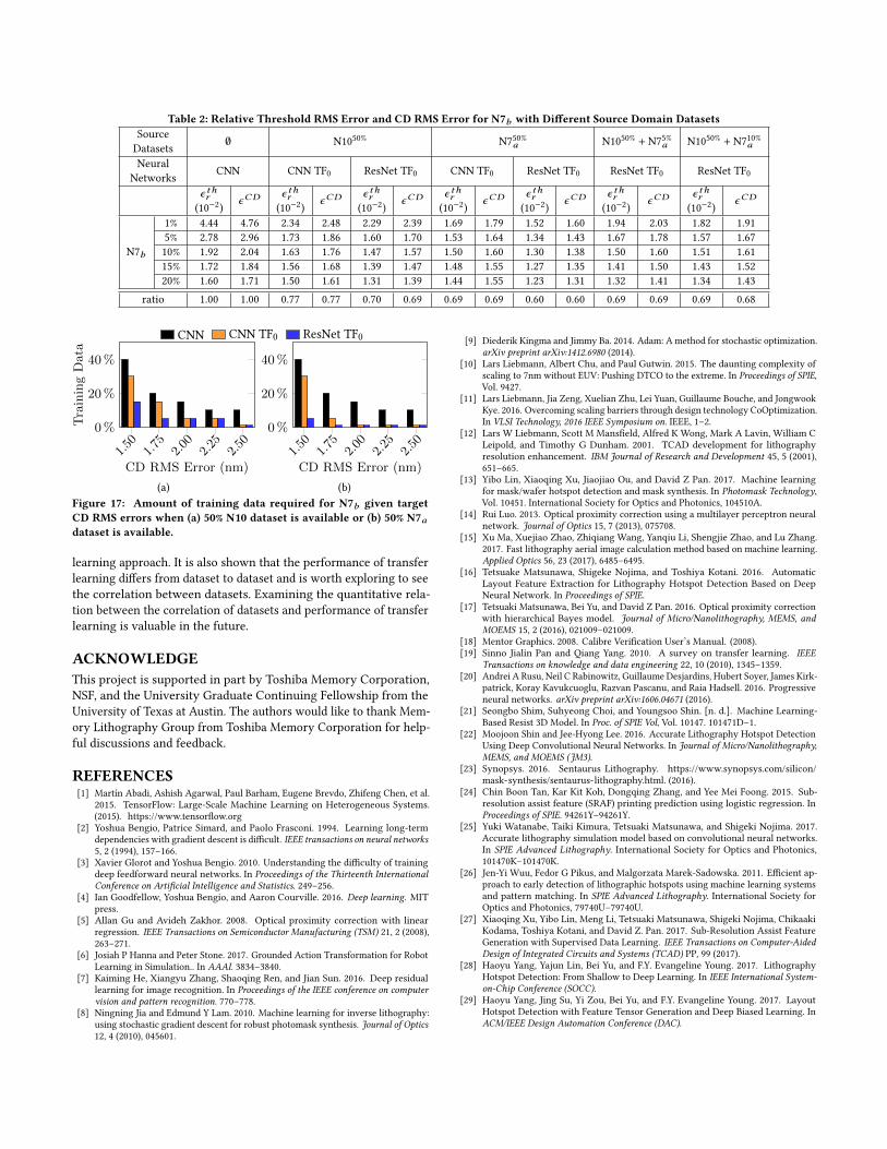
Table 2: Relative Threshold RMS Error and CD RMS Error for N7b with Different Source Domain DatasetsSourceDatasets ∅ N1050% N750%a N1050% + N75%a N1050% + N710%a
NeuralNetworks CNN CNN TF0 ResNet TF0 CNN TF0 ResNet TF0 ResNet TF0 ResNet TF0
ϵ thr(10−2) ϵCD
ϵ thr(10−2) ϵCD
ϵ thr(10−2) ϵCD
ϵ thr(10−2) ϵCD
ϵ thr(10−2) ϵCD
ϵ thr(10−2) ϵCD
ϵ thr(10−2) ϵCD
N7b
1% 4.44 4.76 2.34 2.48 2.29 2.39 1.69 1.79 1.52 1.60 1.94 2.03 1.82 1.915% 2.78 2.96 1.73 1.86 1.60 1.70 1.53 1.64 1.34 1.43 1.67 1.78 1.57 1.6710% 1.92 2.04 1.63 1.76 1.47 1.57 1.50 1.60 1.30 1.38 1.50 1.60 1.51 1.6115% 1.72 1.84 1.56 1.68 1.39 1.47 1.48 1.55 1.27 1.35 1.41 1.50 1.43 1.5220% 1.60 1.71 1.50 1.61 1.31 1.39 1.44 1.55 1.23 1.31 1.32 1.41 1.34 1.43
ratio 1.00 1.00 0.77 0.77 0.70 0.69 0.69 0.69 0.60 0.60 0.69 0.69 0.69 0.68
CNN CNN TF0 ResNet TF0
1.50
1.75
2.00
2.25
2.50
0%
20%
40%
CD RMS Error (nm)
TrainingData
(a)
1.50
1.75
2.00
2.25
2.50
0%
20%
40%
CD RMS Error (nm)
(b)Figure 17: Amount of training data required for N7b given targetCD RMS errors when (a) 50% N10 dataset is available or (b) 50% N7adataset is available.
learning approach. It is also shown that the performance of transferlearning differs from dataset to dataset and is worth exploring to seethe correlation between datasets. Examining the quantitative rela-tion between the correlation of datasets and performance of transferlearning is valuable in the future.
ACKNOWLEDGEThis project is supported in part by Toshiba Memory Corporation,NSF, and the University Graduate Continuing Fellowship from theUniversity of Texas at Austin. The authors would like to thank Mem-ory Lithography Group from Toshiba Memory Corporation for help-ful discussions and feedback.
REFERENCES[1] Martín Abadi, Ashish Agarwal, Paul Barham, Eugene Brevdo, Zhifeng Chen, et al.
2015. TensorFlow: Large-Scale Machine Learning on Heterogeneous Systems.(2015). https://www.tensorflow.org
[2] Yoshua Bengio, Patrice Simard, and Paolo Frasconi. 1994. Learning long-termdependencies with gradient descent is difficult. IEEE transactions on neural networks5, 2 (1994), 157–166.
[3] Xavier Glorot and Yoshua Bengio. 2010. Understanding the difficulty of trainingdeep feedforward neural networks. In Proceedings of the Thirteenth InternationalConference on Artificial Intelligence and Statistics. 249–256.
[4] Ian Goodfellow, Yoshua Bengio, and Aaron Courville. 2016. Deep learning. MITpress.
[5] Allan Gu and Avideh Zakhor. 2008. Optical proximity correction with linearregression. IEEE Transactions on Semiconductor Manufacturing (TSM) 21, 2 (2008),263–271.
[6] Josiah P Hanna and Peter Stone. 2017. Grounded Action Transformation for RobotLearning in Simulation.. In AAAI. 3834–3840.
[7] Kaiming He, Xiangyu Zhang, Shaoqing Ren, and Jian Sun. 2016. Deep residuallearning for image recognition. In Proceedings of the IEEE conference on computervision and pattern recognition. 770–778.
[8] Ningning Jia and Edmund Y Lam. 2010. Machine learning for inverse lithography:using stochastic gradient descent for robust photomask synthesis. Journal of Optics12, 4 (2010), 045601.
[9] Diederik Kingma and Jimmy Ba. 2014. Adam: A method for stochastic optimization.arXiv preprint arXiv:1412.6980 (2014).
[10] Lars Liebmann, Albert Chu, and Paul Gutwin. 2015. The daunting complexity ofscaling to 7nm without EUV: Pushing DTCO to the extreme. In Proceedings of SPIE,Vol. 9427.
[11] Lars Liebmann, Jia Zeng, Xuelian Zhu, Lei Yuan, Guillaume Bouche, and JongwookKye. 2016. Overcoming scaling barriers through design technology CoOptimization.In VLSI Technology, 2016 IEEE Symposium on. IEEE, 1–2.
[12] Lars W Liebmann, Scott M Mansfield, Alfred K Wong, Mark A Lavin, William CLeipold, and Timothy G Dunham. 2001. TCAD development for lithographyresolution enhancement. IBM Journal of Research and Development 45, 5 (2001),651–665.
[13] Yibo Lin, Xiaoqing Xu, Jiaojiao Ou, and David Z Pan. 2017. Machine learningfor mask/wafer hotspot detection and mask synthesis. In Photomask Technology,Vol. 10451. International Society for Optics and Photonics, 104510A.
[14] Rui Luo. 2013. Optical proximity correction using a multilayer perceptron neuralnetwork. Journal of Optics 15, 7 (2013), 075708.
[15] Xu Ma, Xuejiao Zhao, Zhiqiang Wang, Yanqiu Li, Shengjie Zhao, and Lu Zhang.2017. Fast lithography aerial image calculation method based on machine learning.Applied Optics 56, 23 (2017), 6485–6495.
[16] Tetsuake Matsunawa, Shigeke Nojima, and Toshiya Kotani. 2016. AutomaticLayout Feature Extraction for Lithography Hotspot Detection Based on DeepNeural Network. In Proceedings of SPIE.
[17] Tetsuaki Matsunawa, Bei Yu, and David Z Pan. 2016. Optical proximity correctionwith hierarchical Bayes model. Journal of Micro/Nanolithography, MEMS, andMOEMS 15, 2 (2016), 021009–021009.
[18] Mentor Graphics. 2008. Calibre Verification User’s Manual. (2008).[19] Sinno Jialin Pan and Qiang Yang. 2010. A survey on transfer learning. IEEE
Transactions on knowledge and data engineering 22, 10 (2010), 1345–1359.[20] Andrei A Rusu, Neil C Rabinowitz, Guillaume Desjardins, Hubert Soyer, James Kirk-
patrick, Koray Kavukcuoglu, Razvan Pascanu, and Raia Hadsell. 2016. Progressiveneural networks. arXiv preprint arXiv:1606.04671 (2016).
[21] Seongbo Shim, Suhyeong Choi, and Youngsoo Shin. [n. d.]. Machine Learning-Based Resist 3D Model. In Proc. of SPIE Vol, Vol. 10147. 101471D–1.
[22] Moojoon Shin and Jee-Hyong Lee. 2016. Accurate Lithography Hotspot DetectionUsing Deep Convolutional Neural Networks. In Journal of Micro/Nanolithography,MEMS, and MOEMS (JM3).
[23] Synopsys. 2016. Sentaurus Lithography. https://www.synopsys.com/silicon/mask-synthesis/sentaurus-lithography.html. (2016).
[24] Chin Boon Tan, Kar Kit Koh, Dongqing Zhang, and Yee Mei Foong. 2015. Sub-resolution assist feature (SRAF) printing prediction using logistic regression. InProceedings of SPIE. 94261Y–94261Y.
[25] Yuki Watanabe, Taiki Kimura, Tetsuaki Matsunawa, and Shigeki Nojima. 2017.Accurate lithography simulation model based on convolutional neural networks.In SPIE Advanced Lithography. International Society for Optics and Photonics,101470K–101470K.
[26] Jen-Yi Wuu, Fedor G Pikus, and Malgorzata Marek-Sadowska. 2011. Efficient ap-proach to early detection of lithographic hotspots using machine learning systemsand pattern matching. In SPIE Advanced Lithography. International Society forOptics and Photonics, 79740U–79740U.
[27] Xiaoqing Xu, Yibo Lin, Meng Li, Tetsuaki Matsunawa, Shigeki Nojima, ChikaakiKodama, Toshiya Kotani, and David Z. Pan. 2017. Sub-Resolution Assist FeatureGeneration with Supervised Data Learning. IEEE Transactions on Computer-AidedDesign of Integrated Circuits and Systems (TCAD) PP, 99 (2017).
[28] Haoyu Yang, Yajun Lin, Bei Yu, and F.Y. Evangeline Young. 2017. LithographyHotspot Detection: From Shallow to Deep Learning. In IEEE International System-on-Chip Conference (SOCC).
[29] Haoyu Yang, Jing Su, Yi Zou, Bei Yu, and F.Y. Evangeline Young. 2017. LayoutHotspot Detection with Feature Tensor Generation and Deep Biased Learning. InACM/IEEE Design Automation Conference (DAC).