data mining and knowledge discovery handbook || data mining within a regression framework

Chapter 11

DATA MINING WITHIN A REGRESSION FRAMEWORK

Richard A. Berk Department of Statistics UCLA berkOstat.ucla.edu

Abstract Regression analysis can imply a far wider range of statistical procedures than often appreciated. In this chapter, a number of common Data Mining procedures are discussed within a regression framework. These include non-parametric smoothers, classification and regression txees, bagging, and random forests. In each case, the goal is to characterize one or more of the distributional features of a response conditional on a set of predictors.

Keywords: regression, smoothers, splines, CART, bagging, random forests

1. Introduction Regression analysis can imply a broader range of techniques than ordinarily

appreciated. Statisticians commonly define regression so that the goal is to understand "as far as possible with the available data how the the conditional distribution of some response y varies across subpopulations determined by the possible values of the predictor or predictors" (Cook and Weisberg, 1999). For example, if there is a single categorical predictor such as male or female, a legitimate regression analysis has been undertaken if one compares two income histograms, one for men and one for women. Or, one might compare summary statistics from the two income distributions: the mean incomes, the median incomes, the two standard deviations of income, and so on. One might also compare the shapes of the two distributions with a Q-Q plot.

There is no requirement in regression analysis for there to be a "model" by which the data were supposed to be generated. There is no need to address cause and effect. And there is no need to undertake statistical tests or construct confidence intervals. The definition of a regression analysis can be met by pure

232 DATA MINING AND KNOWLEDGE DISCOVERY HANDBOOK

description alone. Construction of a "model," often coupled with causal and statistical inference, are supplements to a regression analysis, not a necessary component (Berk, 2003).

Given such a definition of regression analysis, a wide variety of techniques and approaches can be applied. In this chapter, I will consider a range of procedures under the broad rubric of data mining. The coverage is intended to be broad rather than deep. Readers are encouraged to consult the references cited.

2. Some Definitions There are almost as many definitions of Data Mining as there are trea-

tises on the subject (Sutton and Barto, 1999; Cristianini and Shawe-Taylor, 2000; Witten and Frank, 2000; Hand et al., 2001; Hastie et al., 2001; Breiman, 2001b; Dasu and Johnson, 2003), and associated with Data Mining are a variety of names: statistical learning, machine learning, reinforcement learning, algorithmic modeling and others. By "Data Mining" I mean to emphasize the following.

The broad definition of regression analysis applies. Thus, the goal is to examine ylX for a response y and a set of predictors X, with the values of X treated as fixed. There is no need to commit to any particular feature of ylX, but emphasis will, nevertheless, be placed on the conditional mean, ylX. This is the feature of ylX that has to date drawn the most attention. '

Within the context of regression analysis, now consider a given a data set with N observations, a single predictor x, and a single value of x, xo. The fitted value for $0 at xo can be written as

N

$0 = C s o j ~ j r (11.1) j=1

where S is an N by N matrix of weights, the subscript 0 represents the row corresponding to the case whose value of y is to be constructed, and the subscript j represents the column in which the weight is found. That is, the fitted value Go at xo is linear combination of all N values of y, with the weights determined by Soj . If beyond description, estimation is the goal, one has a linear estimator of ylx. In practice, the weights decline with distance from xo, sometimes abruptly (as in a step function), so that many of the values in Soj are often zero.2

In a regression context, Soj is constructed from a function f (x) that replaces x with transformations of x. Then, we often require that

M

f (XI = C Pmhm (x) (1 1.2) m=l

Regression Framework 233

where there are M transformation of x (which may include the x in its original form and a column of 1's for a constant), pm is the weight given to the mth transformation, and h m ( x ) is the mth transformation of x. Thus, one has a linear combination of transformed values of x. The right hand side is sometime called a "linear basis expansion" in x. Common transformations include polynomial terms, and indicator functions that break x up into several regions. For example, a cubic transformation of x might include three terms: x , x2, x3. An indicator function might be defined so that it equals 1 if x < c and 0 otherwise (where the vector c contains some constant). A key point is that this kind of formulation is both very flexible and computationally tractable.

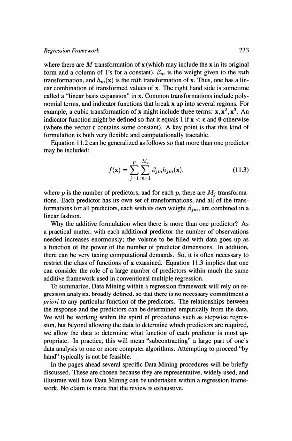
Equation 11.2 can be generalized as follows so that more than one predictor may be included:

where p is the number of predictors, and for each p, there are Mj transformations. Each predictor has its own set of transformations, and all of the transformations for all predictors, each with its own weight pjm, are combined in a linear fashion.

Why the additive formulation when there is more than one predictor? As a practical matter, with each additional predictor the number of observations needed increases enormously; the volume to be filled with data goes up as a function of the power of the number of predictor dimensions. In addition, there can be very taxing computational demands. So, it is often necessary to restrict the class of functions of x examined. Equation 11.3 implies that one can consider the role of a large number of predictors within much the same additive framework used in conventional multiple regression.

To summarize, Data Mining within a regression framework will rely on regression analysis, broadly defined, so. that there is no necessary commitment a priori to any particular function of the predictors. The relationships between the response and the predictors can be determined empirically from the data. We will be working within the spirit of procedures such as stepwise regression, but beyond allowing the data to determine which predictors are required, we allow the data to determine what function of each predictor is most appropriate. In practice, this will mean "subcontracting" a large part of one's data analysis to one or more computer algorithms. Attempting to proceed "by hand" typically is not be feasible.

In the pages ahead several specific Data Mining procedures will be briefly discussed. These are chosen because they are representative, widely used, and illustrate well how Data Mining can be undertaken within a regression framework. No claim is made that the review is exhaustive.


3. Regression Splines A relatively small step beyond conventional parametric regression analysis

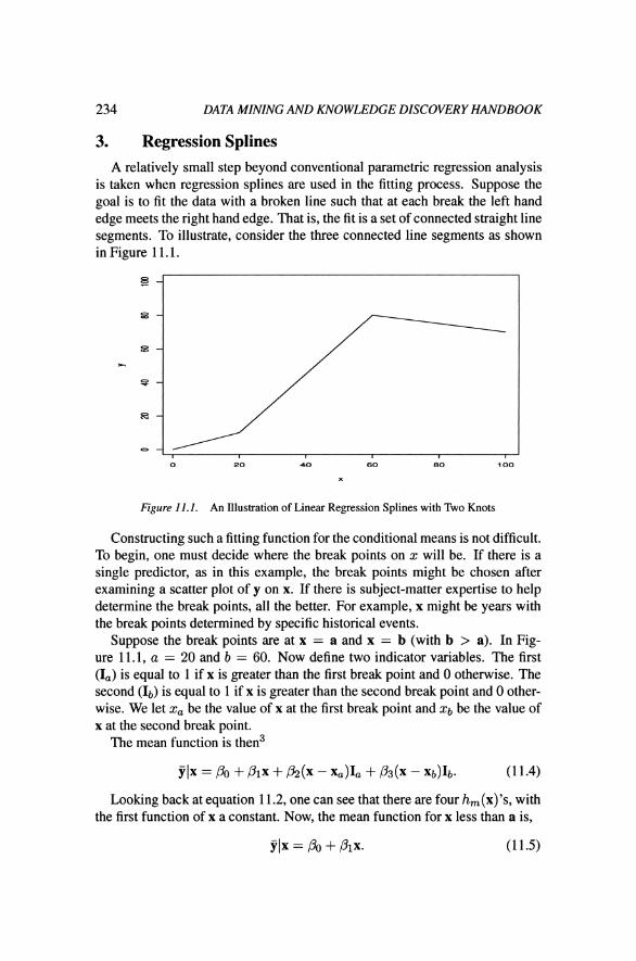
is taken when regression splines are used in the fitting process. Suppose the goal is to fit the data with a broken line such that at each break the left hand edge meets the right hand edge. That is, the fit is a set of connected straight line segments. To illustrate, consider the three connected line segments as shown in Figure 1 1.1.

Figure 11.1. An Illustration of Linear Regression Splines with Two Knots

Constructing such a fitting function for the conditional means is not difficult. To begin, one must decide where the break points on x will be. If there is a single predictor, as in this example, the break points might be chosen after examining a scatter plot of y on x. If there is subject-matter expertise to help determine the break points, all the better. For example, x might be years with the break points determined by specific historical events.

Suppose the break points are at x = a and x = b (with b > a). In Fig- ure 11.1, a = 20 and b = 60. Now define two indicator variables. The first (I,) is equal to 1 if x is greater than the first break point and 0 otherwise. The second (Ib) is equal to 1 if x is greater than the second break point and 0 otherwise. We let x, be the value of x at the first break point and xb be the value of x at the second break point.

The mean function is then3

Looking back at equation 11.2, one can see that there are four h,(x)'s, with the first function of x a constant. Now, the mean function for x less than a is,


For values of x equal to or greater than a but less than b, the mean function is,

YIx = (PO - h x a ) + (P I + P2)x. (1 1.6)

If ,& is positive, for x L a the line is more steep with a slope of (PI + P2) , and lower intercept of (6 - h x a ) . If h is negative, the reverse holds.

For values of x equal to or greater than b, the mean function is,

For values of x greater than b, the slope is altered by adding P3 to the slope of the previous line segment, and the intercept is altered by subtracting P3xb. The sign of P3 determines if the new line segment is steeper or flatter than the previous line segment and where the new intercept falls.

The process of fitting line segments to data is an example of "smoothing" a scatter plot, or applying a "smoother." Smoothers have the goal of constructing fitted values that are less variable than if each of the conditional means of y were connected by a series of broken lines. In this case, one might simply apply ordinary least squares using equation 11.4 as the mean function to compute of the regression parameters. These, in turn, would then be used to construct the fitted values. There would typically be little interpretative interest in the regression'coefficients. The point of the exercise is to superimpose the fitted values on the a scatter plot of the data so that the relationship between y and x can be visualized. The relevant output is the picture. The regression coefficients are but a means to this end.

It is common to allow for somewhat more flexibility by fitting polynomials in x for each segment. Cubic functions of x are a popular choice because they balance well flexibility against complexity. These cubic line segments are known as "piecewise-cubic splines" when used in a regression format and are known as the "truncated power series basis" in spline parlance.

Unfortunately, simply joining polynomial line segments end to end will not produce an appealing fit where the polynomial segments meet. The slopes will often appear to change abruptly even if there is no reason in the data from them to do so. Visual continuity is achieved by requiring that the first derivative and the second derivative on either side of the break points are the same.4

Generalizing from the linear spline framework and keeping the continuity requirement, suppose there are a set of K interior break points, usually called "interior knots," at < . . < EK with two boundary knots at &, and JK+i.

Then, one can use piecewise cubic splines in the following regression formulation:

K

Ylx = PO + PIX + P2x2 + a x 3 + e j ( x - Ej):, (I 1.8) j=1


where the "+" indicates the positive values from the expression, and there are K + 4 parameters to be estimated. This will lead to a conventional regression formulation with a matrix of predictor terms having K + 4 columns and N rows. Each row will have the corresponding values of the piecewise-cubic spline function evaluated at.the single value of x for that case. There is still only a single predictor, but now there are K + 4 transformations.

Fitted values near the boundaries of x for piecewise-cubic splines can be un- stable because they fall at the ends of polynomial line segments where there are no continuity constraints. Sometimes, constraints for behavior at the boundaries are added. One common constraint is that fitted values beyond the boundaries are linear in x. While this introduces a bit of bias, the added stability is often worth it. When these constraints are added, one has "natural cubic splines."

The option of including extra constraints to help stabilize the fit raises the well-known dilemma known as the variance-bias tradeoff. At a descriptive level, a smoother fit will usually be less responsive to the data, but easier to interpret. If one treats y as a random variable, a smoother fit implies more bias because the fitted values will typically be farther from the true conditional means of y ("in the population"), which are the values one wants to estimate from the data on hand. However, in repeated independent random samples (or random realizations of the data), the fitted values will vary less. Conversely, a rougher fit implies less bias but more variance over samples (or realizations), applying analogous reasoning.

For piecewise-cubic splines and natural cubic splines, the degree of smoothness is determined by the number of interior knots. The smaller the number of knots, the smoother the path of the fitted values. That number can be fixed a priori or more likely, determined through a model selection procedure that considers both goodness of fit and a penalty for the number of knots. The Akaike information criterion (AIC) is one popular measure, and the goal is to choose the number of knots that minimizes the AIC. Some software such as as R has procedures that can automate the model selection p ro~ess .~

4. Smoothing Splines There is a way to circumvent the need to determine the number of knots.

Suppose that for a single predictor there is a fitting function f (x) having two continuous derivatives. The goal is to minimize a "penalized" residual sum of squares

where X is a fixed smoothing parameter. The first term captures (as usual) how tight the fit is, while the second imposes a penalty for roughness. The inte-

Regression Framework

Executions

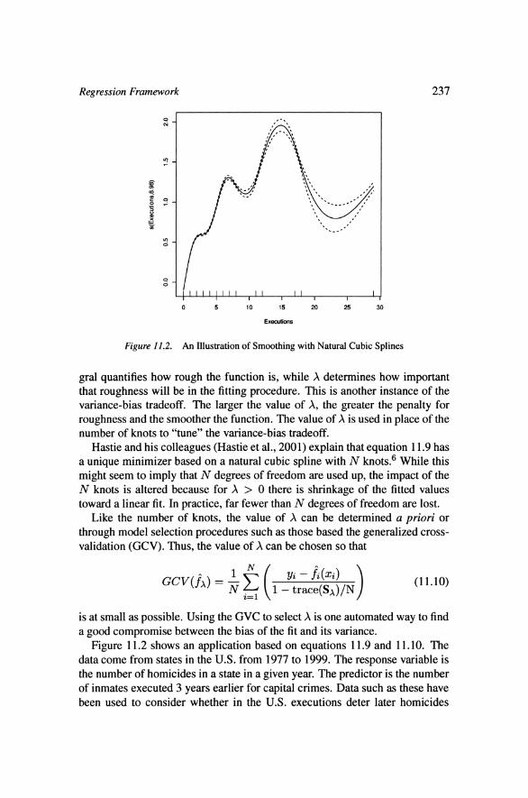
Figure 11.2. An Illustration of Smoothing with Natural Cubic Splines

gral quantifies how rough the function is, while X determines how important that roughness will be in the fitting procedure. This is another instance of the variance-bias tradeoff. The larger the value of A, the greater the penalty for roughness and the smoother the function. The value of X is used in place of the number of knots to "tune" the variance-bias tradeoff.

Hastie and his colleagues (Hastie et al., 2001) explain that equation 11.9 has a unique minimizer based on a natural cubic spline with N knots.6 While this might seem to imply that N degrees of freedom are used up, the impact of the N knots is altered because for X > 0 there is shrinkage of the fitted values toward a linear fit. In practice, far fewer than N degrees of freedom are lost.

Like the number of knots, the value of X can be determined a priori or through model selection procedures such as those based the generalized cross- validation (GCV). Thus, the value of X can be chosen so that

is at small as possible. Using the GVC to select X is one automated way to find a good compromise between the bias of the fit and its variance.

Figure 11.2 shows an application based on equations 11.9 and 11.10. The data come from states in the U.S. from 1977 to 1999. The response variable is the number of homicides in a state in a given year. The predictor is the number of inmates executed 3 years earlier for capital crimes. Data such as these have been used to consider whether in the U.S. executions deter later homicides


(e.g., (Mocan and Gittings, 2003)). Executions are on the horizontal axis (with a rug plot), and homicides are on the vertical axis, labeled as the smooth of executions using 8.98 as the effective degrees of f r e e d ~ m . ~ The solid line is for the fitted values, and the broken lines show the point-by-point 95% confidence interval around the fitted values.

The rug plot at the bottom of Figure 11.2 suggests that most states in most years have very few executions. A histogram would show that the mode is 0. But there are a handful of states that for a given year have a large number of executions (e.g., 18). These few observations are clear outliers.

The fitted values reveal a highly non-linear relationship that generally con- tradicts the deterrence hypotheses when the number of executions is 15 or less; with a larger number of executions, the number of homicides increases the following year. Only when the number of executions is greater than 15 do the fitted values seems consistent with deterrence. Yet, this is just where there is almost no data. Note that the confidence interval is much wider when the number of executions is between 18 and 28.8

The statistical message is that the relationship between the response and the predictor was derived directly from the data. No functional form was imposed a priori. And none of the usual regression parameters are reported. The story is Figure 11.2. Sometimes this form of regression analysis is called "nonparametric regression."

5. Locally Weighted Regression as a Smoother Spline smoothers are popular, but there are other smoothers that are widely

used as well. Lowess is one example (Cleveland, 1979). Lowess stands for "locally weighted linear regression smoother."

Consider again the one predictor case. The basic idea is that for any given value of the predictor xo, a linear regression is constructed from observations with x-values near xo. These data are weighted so that observations with x- values closer to xo are given more weight. Then, is computed from the fitted regression line and used as the smoothed value of the response at xo. This process is then repeated for all other x-values.

The precise weight given to each observation depends on the weighting function employed; the normal distribution is one option? The degree of smoothing depends on the proportion of the total number of observations used when each local regression line is constructed. The larger the "window" or "span," the larger the proportion of observations included, and the smoother the fit. Proportions between .25 and .75 are common because they seem to provide a good balance for the variance-bias tradeoff.


More formally, each local regression derives from minimizing the weighted sum of squares with respect to the intercept and slope for the M < N observations included in the window. That is,

RSS* (P) = (y* - x*P)~w*(~* - X*P),

where the asterisk indicates that only the observations in the window are included, and W* is an M x M diagonal matrix with diagonal elements w;, which are a function of distance from xo. The algorithm then operates as follows.

1. Choose the smoothing parameter f, which a proportion between 0 and 1.

2. Choose a point xo and from that the (f x N = M) nearest points on x.

3. For these "nearest neighbor" points, compute a weighted least squares regression line for y on x.

4. Construct the fitted value go for that single xo.

5. Repeat steps 2 through 4 for each value of x.1°

6. Connect these gs with a line.

Lowess is a very popular smoother when there is a single predictor. With a judicious choice of the window size, Figure 11.2 could be effectively reproduced.

6. Smoothers for Multiple Predictors In principle, it is easy to add more predictors and then smooth a multidi-

mensional space. However, there are three major complications. First, there is the "curse of dimensionality." As the number of predictors increases, the space that needs to be filled with data goes up as a power function. So, the demand for data increases rapidly, and the risk is that the data will be far too sparse to get a meaningful fit.

Second, there are some difficult computational issues. For example, how is the neighborhood near xo to be defined when predictors are correlated? Also, if the one predictor has much more variability than another, perhaps because of the units of measurement, that predictor can dominate the definition of the neighborhood.

Third, there are interpretative difficulties. When there are more than two predictors one can no longer graph the fitted surface. How then does one make sense of a surface in more than three dimensions?


When there are only two predictors, there are some fairly straightforward extensions of conventional smoothers that can be instructive. For example, with smoother splines, the penalized sum of squares in equation 11.9 can be generalized. The solution is a set of "thin plate splines," and the results can be plotted. With more than two predictors, however, one generally need another strategy. The generalized additive model is one popular strategy that meshes well with the regression emphasis in this chapter.

6.1 The Generalized Additive Model The mean function for generalized additive model (GAM) with p predictors

can is written as P

7 1 ~ = CY + C f j ( x j ) . (11.12) j=l

Just as the generalized linear model (GLM), the generalized additive model allows for a number of "link functions" and disturbance distributions. For example, with logistic regression the link function is the log of the odds (the "logit") of the response, and disturbance distribution is logistic.

Each predictor is allowed to have its own functional relationship to the response, with the usual linear form as a special case. If the former, the functional form can be estimated from the data or specified by the researcher. If the latter, all of the usual regression options are available, including indicator variables. Functions of predictors that are estimated from the data rely on smoothers of the sort just d i s c ~ s s e d . ~ ~

With the additive form, one can use the same general conception of what it means to "hold constant" that applies to conventional linear regression. The fitting algorithm GAM removes linear dependence between predictors in a fashion that is analogous to the matrix operations behind conventional least squares estimates.

6.1.1 A GAM Fitting Algorithm. Many software packages use the backfitting algorithm to estimate the functions and constant in equation 1 1.12 (Hastie and Tibshirani, 1990). The basic idea is not difficult and proceeds in the following steps.

1. Initialize: CY = pi, f j = f:, j = 1, . . . , p. Each predictor is given an initial functional relationship to the response such as a linear one. The intercept is given an initial value of the mean of y.

2. Cycle: j = 1 , . . . , p , 1 , . . . , p , . . .


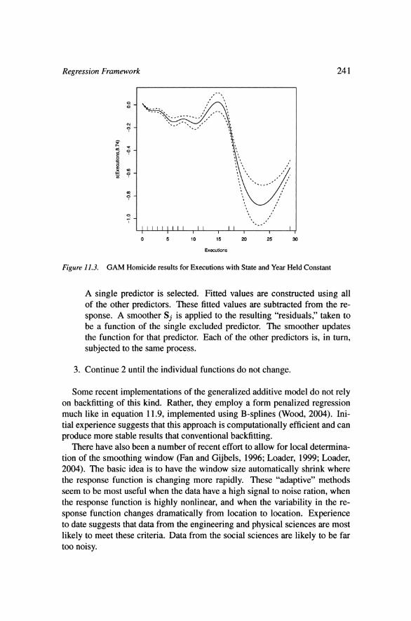
Figure 11.3. GAM Homicide results for Executions with State and Year Held Constant

A single predictor is selected. Fitted values are constructed using all of the other predictors. These fitted values are subtracted from the response. A smoother Sj is applied to the resulting "residuals," taken to be a function of the single excluded predictor. The smoother updates the function for that predictor. Each of the other predictors is, in turn, subjected to the same process.

3. Continue 2 until the individual functions do not change.

Some recent implementations of the generalized additive model do not rely on backfitting of this kind. Rather, they employ a form penalized regression much like in equation 11.9, implemented using B-splines (Wood, 2004). Ini- tial experience suggests that this approach is computationally efficient and can produce more stable results that conventional backfitting.

There have also been a number of recent effort to allow for local determina- tion of the smoothing window (Fan and Gijbels, 1996; Loader, 1999; Loader, 2004). The basic idea is to have the window size automatically shrink where the response function is changing more rapidly. These "adaptive" methods seem to be most useful when the data have a high signal to noise ration, when the response function is highly nonlinear, and when the variability in the response function changes dramatically from location to location. Experience to date suggests that data from the engineering and physical sciences are most likely to meet these criteria. Data from the social sciences are likely to be far too noisy.


Consider now an application of the generalized additive model. For data described earlier, Figure 11.3 shows the relationship between number of homicides and the number executions a year earlier, with state and year held constant. Indicator variables are included for each state to adjust for average differences over time in the number of homicides in each state. For example, states differ widely in population size, which is clearly factor in the raw number of homicides. Indicator variables for each state control for such differences. In- dicator variables for year are included to adjust for average differences across states in the number of homicides each year. This controls for year to year trends for the country as a whole in the number of homicides.

There is now no apparent relationship between executions and homicides a year later except for the handful of states that in a very few years had a large number of executions. Again, any story is to be found in a few extreme outliers that are clearly atypical. The statistical point is that one can accommodate with GAM both smoother functions and conventional regression functions.

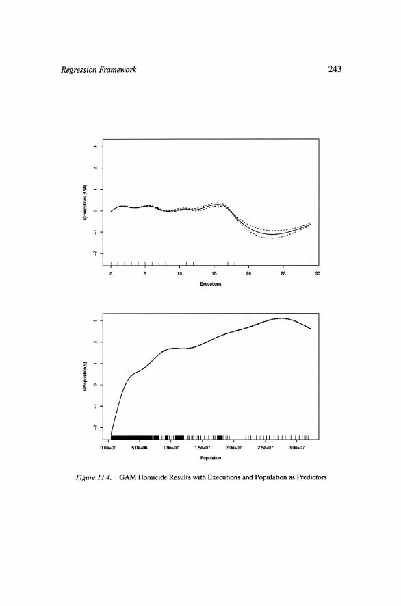
Figure 11.4 shows the relationship between number of homicides and 1) the number executions a year earlier and 2) the population of each state for each year. The two predictors were included in an additive fashion with their functions determined by smoothers.

The role of execution is about the same as in Figure 11.3, although at first glance the new vertical scale makes it looks a bit different. In addition, one can see that homicides increase monotonically with population size, as one would expect, but the rate of increase declines. The very largest states are not all that different from middle sized states.

7. Recursive Partitioning Recall again equation 11.3 reproduced below for convenience as equation

11.14:

An important special case sequentially includes basis functions that con- tribute to substantially to the fit. Commonly, this is done in much the same spirit as forward selection methods in stepwise regression. But, there are now two components to the fitting process. A function for each predictor is constructed. Then, only some of these functions are determined to be worthy and included in the final model. Classification and Regression Trees (Breiman et al., 1984), commonly known as CART, is probably the earliest and most well known example of this approach.


Figure 11.4. GAM Homicide Results with Executions and Population as Predictors


7.1 Classification and Regression Trees and Extensions CART can be applied to both categorical and quantitative response vari-

ables. We will consider first categorical response variables because they provide a better vehicle for explaining how CART functions.

CART uses a set of predictors to partition the data so that within each partition the values of the response variable are as homogeneous as possible. The data are partitioned one partition at a time. Once a partition is defined, it is unaffected by later partitions. The partitioning is accomplished with a series of straight-line boundaries, which define a break point for each selected predictor. Thus, the transformation for each predictor is an indicator variable.

Figure 11.5 illustrates a CART partitioning. There is a binary outcome coded "A" or "B" and in this simple illustration, just two predictors, x and z, are selected. The single vertical line defines the first partition. The double horizontal line defines the second partition. The triple horizontal line defines the third partition.

The data are first segmented left from right and then for the two resulting partitions, the data are further segmented separately into an upper and lower part. The upper left partition and the lower right partition are perfectly homogeneous. There remains considerable heterogeneity in the other two partitions and in principle, their partitioning could continue. Nevertheless, cases that are high on z and low on x are always "B." Cases that are low on z and high on x are always "A." In a real analysis, the terms "high" and "low" would be precisely defined by where the boundaries cross the x and z axes.

The process by which each partition is constructed depends on two steps. First, each potential predictor individually is transformed into the indicator variable best able to split the data into two homogenous groups. All possible break points for each potential predictor are evaluated. Second, the predictor with the most effective indicator variable is selected for construction of the partition. For each partition, the process is repeated with all predictors, even ones used to construct earlier partitions. As a result, a given predictor can be used to construct more than one partition; some predictors will have more than one transformation selected.

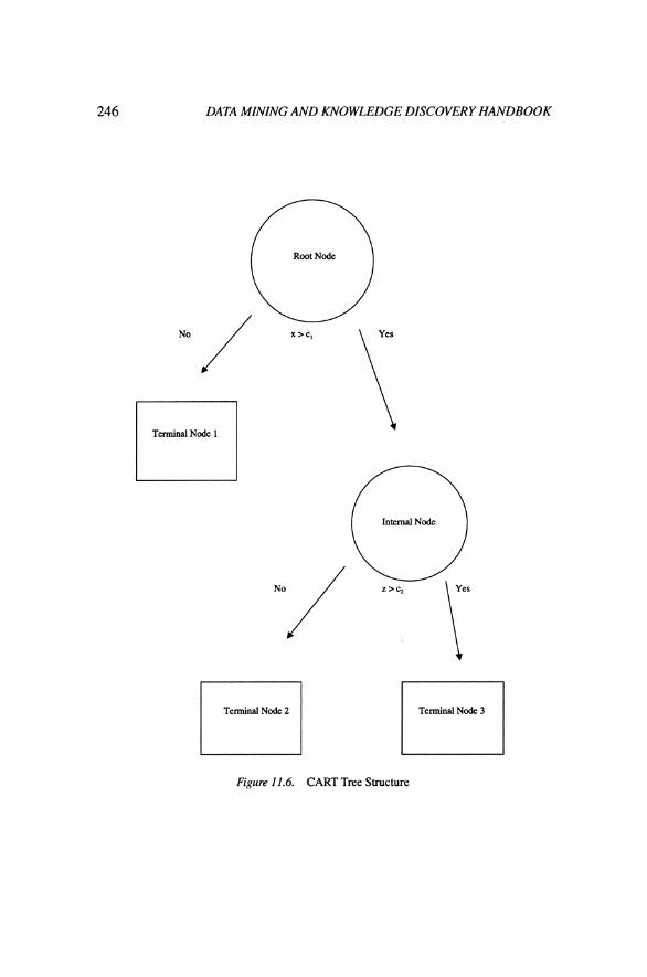
Usually, CART output is displayed as an inverted tree. Figure 11.6 is a simple illustration. The full data set is contained in the root node. The final partitions are subsets of the data placed in the terminal nodes. The internal nodes contain subsets of data for intermediate steps.

To achieve as much homogeneity as possible within data partitions, heterogeneity within data partitions is minimized. Two definitions of heterogeneity that are especially common. Consider a response that is a binary variable coded 1 or 0. Let the "impurity" i of node T be a non-negative function of the proba- bility that y = 1. If T is a node composed of cases that are all 1's or all O's, its


Recursive Partitioning of a Binary Outcome (whereY = A or B and predictors are Z and X)

Figure 11.5. Recursive Partitioning Logic in CART

DATA MINING AND KNOWLEDGE DISCOVERY HANDBOOK

Terminal Node 1

Root Node

Terminal Node 2 El Terminal Node 3 El Figure 11.6. CART Tree Structure


impurity is 0. If half the cases are 1's and half the cases are O's, T is the most impure it can be. Then, let

where 4 2 0, $(p) = $(1 - p) , and +(0) = + ( I ) < $(p ) . Impurity is non-negative, symmetrical, and is at a minimum when all of the cases in T

are of one kind or another. The two most common options for the function 4 are the entropy function shown in equation 11.16 and the Gini Index shown in equation 1 1. 17:12

Both equations are concave with minimums at p = 0 and p = 1 and a maximum at p = .5. CART results from the two are often quite similar, but the Gini index seems to perform a bit better, especially when there are more than two categories in the response variable.

While it may not be immediately apparent, entropy and the Gini index are in much same spirit as the least squares criterion commonly use in regression, and the goal remains to estimate a set of conditional means. Because in classification problems the response can be coded as a 1 or a 0, the mean is a proportion.

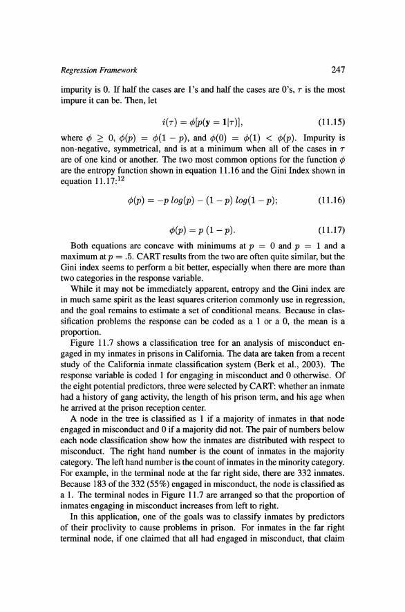
Figure 11.7 shows a classification tree for an analysis of misconduct engaged in my inmates in prisons in California. The data are taken from a recent study of the California inmate classification system (Berk et al., 2003). The response variable is coded 1 for engaging in misconduct and 0 otherwise. Of the eight potential predictors, three were selected by CART: whether an inmate had a history of gang activity, the length of his prison term, and his age when he arrived at the prison reception center.

A node in the tree is classified as 1 if a majority of inmates in that node engaged in misconduct and 0 if a majority did not. The pair of numbers below each node classification show how the inmates are distributed with respect to misconduct. The right hand number is the count of inmates in the majority category. The left hand number is the count of inmates in the minority category. For example, in the terminal node at the far right side, there are 332 inmates. Because 183 of the 332 (55%) engaged in misconduct, the node is classified as a 1. The terminal nodes in Figure 1 1.7 are arranged so that the proportion of inmates engaging in misconduct increases from left to right.

In this application, one of the goals was to classify inmates by predictors of their proclivity to cause problems in prison. For inmates in the far right terminal node, if one claimed that all had engaged in misconduct, that claim

DATA MINING AND KNOWLEDGE DISCOVERY HANDBOOK

Figure 11.7. Classification Tree for Inmate Misconduct

would be incorrect 44% of the time. This is much better than one would do ignoring the predictors. In that case, if one claimed that all inmates engaged in misconduct, that claim would be wrong 79% of the time.

The first predictor selected was gang activity. The "a" indicates that the inmates with a history of gang activity were placed in the right node, and inmates with a history of no gang activity were placed in the left node. The second predictor selected was only able meaningfully to improve the fit for inmates with a history of gang activity. Inmates with a sentence length ("Term") of less than 2.5 years were assigned to the left node, while inmates with a sentence length of 2.5 years or more were assigned to the right node. The final variable selected was only able meaningfully to improve the fit for the subset of inmates with a history of gang activity who were serving longer prison terms. That variable was the age of the inmate when he arrived at the prison reception center. In- mates with ages greater than 25 (age categories b, c, and d) were assigned to the left node, while inmates with ages less than 25 were assigned to the right node. In the end, this sorting makes good subject-matter sense. Prison officials often expect more trouble from younger inmates with a history of gang activity serving long terms.

When CART is applied with a quantitative response variable, the procedure is known as "Regression Trees." At each step, heterogeneity is now measured


by the within-node sum of squares of the response:

where for node T the summation is over all cases in that node, and V(T) is the mean of those cases. The heterogeneity for each potential split is the sum of the two sums of squares for the two nodes that would result. The split is chosen that reduces most this within-nodes sum of squares; the sum of squares of the parent node is compared to the combined sums of squares from each potential split into two offspring nodes. Generalization to Poisson regression (for count data) follows with the deviance used in place of the sum of squares.

7.2 Overfitting and Ensemble Methods CART, like most Data Mining procedures, is vulnerable to overfitting. Be-

cause the fitting process is so flexible, the mean function tends to "over- respond" to idiosyncratic features of the data. If the data on hand are a random sample for a particular population, the mean function constructed from the sample can look very different from the mean function in the population (were it known). One implication is that a different random sample from the same population can lead to very different characterizations of how the response is related to the predictors. Conventional responses to overfitting (e.g., model selection based on the AIC) are a step in the right direction. However, they are often not nearly strong enough and usually provide few clues how a more appropriate model should be constructed.

It has been known for nearly a decade that one way to more effectively coun- teract overfitting is to construct average results over a number of random samples of the data (LeBlanc and Tibshirani, 1996; Mojirsheibani, 1999; Friedman et al., 2000). Cross-validaton can work on this principle. When the samples are bootstrap samples from a given data set, the procedures are sometimes called ensemble methods, with "bagging" as an early and important special case (Breiman, 1996).13 Bagging can be applied to a wide variety of fitting procedures such as conventional regression, logistic regression and discrimi- nant function analysis. Here the focus will be on bagging regression and classification trees.

The basic idea is that the various manifestations of overfitting cancel out in the aggregate over a large number of independent random samples from the same population. Bootstrap samples from the data on hand provide a surrogate for independent random samples from a well-defined population. However, the bootstrap sampling with replacement implies that bootstrap samples will share some observations with one another and that, therefore, the sets of fitted values across samples will not be independent. A bit of dependency is built it.


For recursive partitioning, the amount of dependence can be decreased substantially if in addition to random bootstrap samples, potential predictors are randomly sampled (with replacement) at each step. That is, one begins with a bootstrap sample of the data having the same number of observations as in the original data set. Then, when each decision is made about subdividing the data, only a random sample of predictors is considered. The random sample of predictors at each split may be relatively small (e.g., 5).

"Random forests" is one powerful approach exploiting these ideas. It builds on CART, and will generally fit the data better than standard regression models or CART itself (Breiman, 2001a). A large number of classification or regression trees is built (e.g., 500). Each tree is based on a bootstrap sample of the data on hand, and at each potential split, a random sample of predictors is considered. Then, average results are computed over the full set of trees. In the binary classification case, for example, a "vote" is taken over all of the trees to determine if a given case is assigned to one class or the other. So, if there are 500 trees and in 25 1 or more of these trees that case is classified as a "1," that case is treated as a "1 ."

One problem with random forests is that there is no longer a tree to interpret.14 Partly in response to this defect, there are currently several methods under development that attempt to represent the importance of each predictor for the average fit. Many build on the following approach. The random forests procedure is applied to the data. For each tree, observations not included in the bootstrap sample are used as a "test" data set.15 Some measure of the quality of the fit is computed with these data. Then, the values of a given explanatory variable in the test data are randomly shuffled, and a second measure of fit quality computed. Each of the measures is then averaged across the set of constructed trees. Any substantial decrease in the quality of the fit when the average of the first is compared to the average of the second must result from eliminating the impact of the shuffled variable.16 The same process is repeated for each explanatory variable in turn.

There is no resolution to date of exactly what feature of the fit should be used to judge the importance of a predictor. Two that are commonly employed are the mean decline over trees in the overall measure of fit (e.g. the Gini Indix) and for classification problems, the mean decline over trees in how accurately cases are predicted. For example, suppose that for the full set explanatory variables an average of 75% of the cases are correctly predicted. If after the values of a given explanatory variable are randomly shuffled that figure drops to 65%, there is a reduction in predictive accuracy of 10%. Sometimes a standardized decline in predictive accuracy is used, which may be loosely interpreted as a z-score.

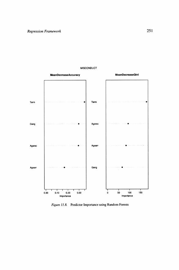
Figure 11.8 shows for the prison misconduct data how one can consider predictor importance using random forests. The number of explanatory vari-


MISCONDUCT

, , , , , , I0 0.10 0.20 0.30

Importance

Term

Agerec

Agearr

Gang

Figure 11.8. Predictor Importance using Random Forests


ables included in the figure is truncated at four for ease of exposition. Term length is the most important explanatory variable by both the predictive accuracy and Gini measures. After that, the rankings from the two measures vary. Disagreements such as these are common because the Gini Index reflects the overall goodness of fit, while the predictive accuracy depends on how well the model actually predicts. The two are related, but they measure different things. Breiman argues that the decrease in predictive accuracy is the more direct, stable and meaningful indicator of variable importance (personal communica- tion). If the point is to accurately predict cases, why not measure importance by that criterion? In that case, the ranking of variables by importance is term length, gang activity, age at reception, and age when first arrested.

When the response variable is quantitative, importance is represented by the average increase in the within node sums of squares for the terminal nodes. The increase in this error sum of squares is related to how much the "explained variance" decreases when the values of a given predictor are randomly shuffled. There is no useful analogy in regression trees to correct or incorrect prediction.

8. Conclusions A large number of Data Mining procedures can be considered within a re-

gression framework. A representative sample of the most popular and powerful has been discussed in this chapter.17 With more space, others could have been included: boosting (Freund and Schapire, 1995) and support vector machines (Vapnik, 1995) are two obvious candidates. Moreover, the development of new data mining methods is progressing very quickly, stimulated in part by relatively inexpensive computing power and in part by the Data Mining needs in a variety of disciplines. A revision of this chapter five years from now might look very different. Nevertheless, a key distinction between the more effective and the less effective Data Mining procedures is how overfitting is handled. Finding new and improved. ways to fit data is often quite easy. Finding ways to avoid being seduced by the results is not (Svetnik et al., 2003; Reunanen, 2003).

Acknowledgments The final draft of this chapter was funded in part by a grant from the National

Science Foundation: (SES -0437 169) "Ensemble methods for Data Analysis in the Behavioral, Social and Economic Sciences." This chapter was completed while visiting at the Department of Earth, Atmosphere, and Oceans, at the Ecole Normale Sup6rieur in Paris. Support from both is gratefully acknowl- edged.


Notes 1. In much of what follows I use the framework presented in (Hastie et al., 2001). Generally, matrices

will be shown in capital letters in bold face type, vectors will be shown in small letters with bold face type, and scalars will be shown in small letter in italics. But by and large, the meaning will be clear from the context

2. It is the estimator that is linear. The function linking the response variable y to the predictor x can be highly non-linear. The role of Soj has much in common the hat-matrix from conventional linear regression analysis: H = x ( x * x ) - ' x ~ . The hat-matrix transforms y, in a linear fashion into 9,. Soj does the same thing but can be constructed in a more general manner.

3. To keep the equations consistent with the language of the text and to emphasize the descriptive nature of the enterprise, the conditional mean of y will be represented by 7-x rather than by E ( y J x ) . The latter implies, unnecessarily in this case, that y is a random variable.

4. This is not a formal mathematical result. It stems from what seems to he the kind of smoothness the human eye can appreciate.

5. In practice, the truncated power series basis is usually replaced by a B-spline basis. That is, the transformations of x required are constructed from another basis, not explicit cubic functions of x. In brief, all splines are linear combinations of B-splines; B-splines are a basis for the space of splines. They are also a well-conditioned basis, because they are fairly close to orthogonal, and they can be computed in a stable and efficient manner. Good discussions of B-splines can be found in (Gifi, 1990) and (Hastie et al., 2001).

6. This assumes that there are N distinct values of x. There will be fewer knots if there are less than N distinct values of x .

7. The effective degrees of freedom is the degrees of freedom required by the smoother, and is calcu- lated as the trace of S in equation 11.1. It is analogous to the degrees of freedom "used up" in a conventional linear regression analysis when the intercept and regression coefficients are computed. The smoother the fitted value, the greater the effective degrees of freedom used.

8. Consider again equations 11.1 and 11.2. The natural cubic spline values for executions are the hm ( x ) in equation 11.2 which, in turn is the source of S. From S and the number of homicides y ones obtains the fitted values j shown in Figure 11.2.

9. The tricube is another popular option. In practice, most of the common weighting functions give about the same results.

10. As one approaches either tail of the distribution of x, the window will tend to become asymmetrical. One implication is that the fitted values derived from x-values near the tails of x are typically less stable. Additional constraints are then sometimes imposed much like those imposed on cubic splines.

11. The functions constructed from the data are built so that they have a mean of zero. When all of the functions are estimated from the data, the generalized additive model is sometimes cal1ed"nonparametric." When some of the functions are estimated from the data and some are determined by the researcher, the generalized additive model is sometimes called "semiparametric."

12. Both can he generalized for nominal response variables with more than two categories (Hastie et al., 2001).

13. "Bagging" stands for bootstrap aggregation. 14. More generally, ensemble methods can lead to difficult interpretative problems if the links of inputs

to outputs are important to describe. 15. These are sometimes called "out-of-bag" observations. "Predicting" the values of the response

for observations used to build the set of trees will lead to overly optimistic assessments of how well the procedure performs. Consequently, out-of-bag (OOB) observations are routinely used in random forests to determine how well random forests predicts.

16. Small decreases could result from random sampling error. 17. All of the procedures described in this chapter can be easily computed with procedures found in the

programming language R.

References Berk, R.A. (2003) Regression Analysis: A Constructive Critique. Newbury

Park, CA.: Sage Publications.


Berk, R.A., Ladd, H., Graziano, H., and J. Baek (2003) "A Randomized Exper- iment Testing Inmate Classification Systems," Journal of Criminology and Public Policy, 2, No. 2: 215-242.

Breiman, L., Friedman, J.H., Olshen, R.A., and C.J. Stone, (1984) Classifica- tion and Regression Trees. Monterey, Ca: Wadsworth Press.

Breiman, L. (1996) "Bagging Predictors." Machine Learning 26:123-140. Breiman, L. (2000) "Some Infinity Theory for Predictor Ensembles." Technical

Report 522, Department of Statistics, University of California, Berkeley, California.

Breiman, L. (2001a) "Random Forests." Machine Learning 45: 5-32. Breiman, L. (2001b) "Statistical Modeling: Two Cultures," (with discussion)

Statistical Science 16: 199-23 1. Cleveland, W. (1979) "Robust Locally Weighted Regression and Smoothing

Scatterplots." Journal of the American Statistical Association 78: 829-836. Cook, D.R. and Sanford Weisberg (1999) Applied Regression Including Com-

puting and Graphics. New York: John Wiley and Sons. Dasu, T., and T. Johnson (2003) Exploratory Data Mining and Data Cleaning.

New York: John Wiley and Sons. Christianini, N and J. Shawe-Taylor. (2000) Support Vector Machines. Cam-

bridge, England: Cambridge University Press. Fan, J., and I. Gijbels. (1996) Local Polynomial Modeling and its Applications.

New York: Chapman & Hall. Friedman, J., Hastie, T., and R. Tibsharini (2000). "Additive Logistic Regres-

sion: A Statistical View of Boosting" (with discussion). Annals of Statistics 28: 337-407.

Freund, Y., and R. Schapire. (1996) "Experiments with a New Boosting Al- gorithm," Machine Learning: Proceedings of the Thirteenth International Conference: 148-156. San Francisco: Morgan Freeman

Gigi, A. (1990) Nonlinear Multivariate Analysis. New York: John Wiley and Sons.

Hand, D., Manilla, H., and P Smyth (2001) Principle of Data Mining. Cam- bridge, Massachusetts: MIT Press.

Hastie, T.J. and R.J. Tibshirani. (1990) Generalized Additive Models. New York: Chapman 62 Hall.

Hastie, T., Tibshirani, R. and J. Friedman (2001) The Elements of Statistical Learning. New York: Springer-Verlag.

LeBlanc, M., and R. Tibshirani (1996) "Combining Estimates on Regression and Classification." Journal of the American Statistical Association 91: 1641-1650.

Loader, C. (1999) Local Regression and Likelihood. New York: Springer- Verlag.


Loader, C. (2004) "Smoothing: Local Regression Techniques," in J. Gentle, W. Hiirdle, and Y. Mori, Handbook of Computational Statistics. NewYork: Springer-Verlag.

Mocan, H.N. and K. Gittings (2003) "Getting off Death Row: Commuted Sen- tences and the Deterrent Effect of Capital Punishment." (Revised version of NBER Working Paper No. 8639) and forthcoming in the Journal of Law and Economics.

Mojirsheibani, M. (1999) "Combining Classifiers vis Discretization." Journal of the American Statistical Association 94: 600-609.

Reunanen, J. (2003) "Overlitting in Making Comparisons between Variable Selection Methods." Journal of Machine Learning Research 3: 1371-1382.

Sutton, R.S., and A.G. Barto. (1999). Reinforcement Learning. Cambridge, Massachusetts: MIT Press.

Svetnik, V., Liaw, A., and C.Tong. (2003) "Variable Selection in Random For- est with Application to Quantitative Structure-Activity Relationship." Work- ing paper, Biometries Research Group, Merck & Co., Inc.

Vapnik, V. (1995) The Nature of Statistical Learning Theory. New York: Springer-Verlag.

Witten, I.H. and E. Frank. (2000). Data Mining. New York: Morgan and Kauf- mann.

Wood, S.N. (2004) "Stable and Eficient Multiple Smoothing Parameter Esti- mation for Generalized Additive Models," Journal of the American Statisti- cal Association, Vol. 99, No. 467: 673-686.

data mining and knowledge discovery handbook || data mining within a regression framework

Documents