data mining and knowledge discovery - ijskt.ijs.si/petrakralj/ips_dm_1516/dm-2015.pdf · data...
TRANSCRIPT

Data Mining
and Knowledge Discovery
Part of
Jožef Stefan IPS Programme - ICT3
and UL Programme - Statistics
2015 / 2016
Nada Lavrač
Jožef Stefan Institute
Ljubljana, Slovenia
2
Jožef Stefan Institute and IPS
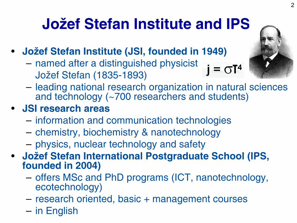
• Jožef Stefan Institute (JSI, founded in 1949)
– named after a distinguished physicist
Jožef Stefan (1835-1893)
– leading national research organization in natural sciences and technology (~700 researchers and students)
• JSI research areas
– information and communication technologies
– chemistry, biochemistry & nanotechnology
– physics, nuclear technology and safety
• Jožef Stefan International Postgraduate School (IPS, founded in 2004)
– offers MSc and PhD programs (ICT, nanotechnology, ecotechnology)
– research oriented, basic + management courses
– in English
3
Jožef Stefan Institute
Department of Knowledge Technologies
• Head: Nada Lavrač, Staff: 30 researchers, 10 students
• Machine learning & Data mining – ML (decision tree and rule learning, subgroup discovery, …)
– Text and Web mining
– Relational data mining - inductive logic programming
– Equation discovery
• Other research areas: – Knowledge management
– Decision support
– Human language technologies
• Applications: – Medicine, Bioinformatics, Public Health
– Ecology, Finance, …
4
Course Outline
I. Introduction
– Data Mining in a Nutshell
– Predictive and descriptive DM techniques
– Data Mining and KDD process
– DM standards, tools and visualization
(Mladenić et al. Ch. 1 and 11)
II. Predictive DM Techniques
– Bayesian classifier (Kononenko Ch. 9.6)
– Decision Tree learning
(Mitchell Ch. 3, Kononenko Ch. 9.1)
– Classification rule learning (Kononenko Ch. 9.2)
– Classifier Evaluation
(Bramer Ch. 6)
III. Regression
(Kononenko Ch. 9.4)
IV. Descriptive DM
– Predictive vs. descriptive induction
– Subgroup discovery
– Association rule learning (Kononenko Ch. 9.3)
– Hierarchical clustering (Kononenko Ch. 12.3)
– V. Relational Data Mining
– RDM and Inductive Logic Programming (Dzeroski & Lavrac Ch. 3, Ch. 4)
– Propositionalization approaches
– Relational subgroup discovery
5
Part I. Introduction
• Data Mining in a Nutshell
• Predictive and descriptive DM techniques
• Data Mining and the KDD process
• DM standards, tools and visualization
6
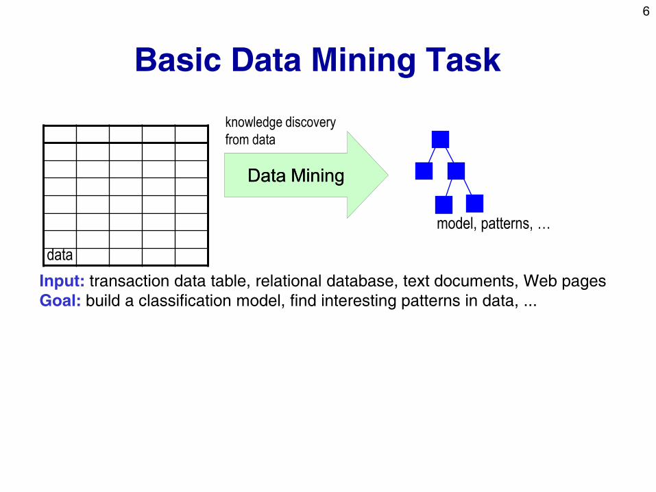
Basic Data Mining Task
data
Data MiningData Mining
knowledge discovery
from data
model, patterns, …
Input: transaction data table, relational database, text documents, Web pages
Goal: build a classification model, find interesting patterns in data, ...
7
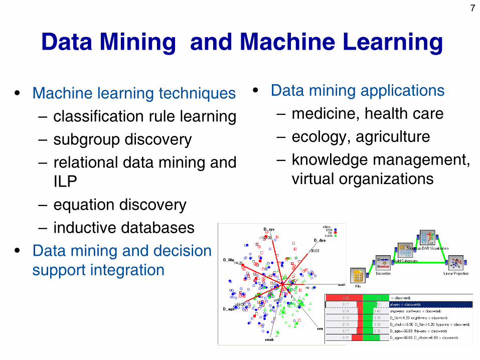
Data Mining and Machine Learning
• Machine learning techniques
– classification rule learning
– subgroup discovery
– relational data mining and
ILP
– equation discovery
– inductive databases
• Data mining and decision
support integration
• Data mining applications
– medicine, health care
– ecology, agriculture
– knowledge management,
virtual organizations
8
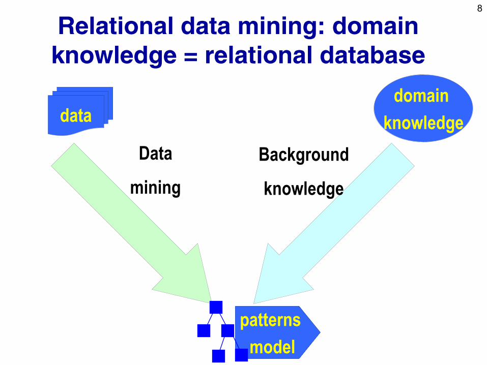
Relational data mining: domain
knowledge = relational database
Data
mining
Background
knowledge
patterns
odel
patterns
model
data domain
knowledge
9
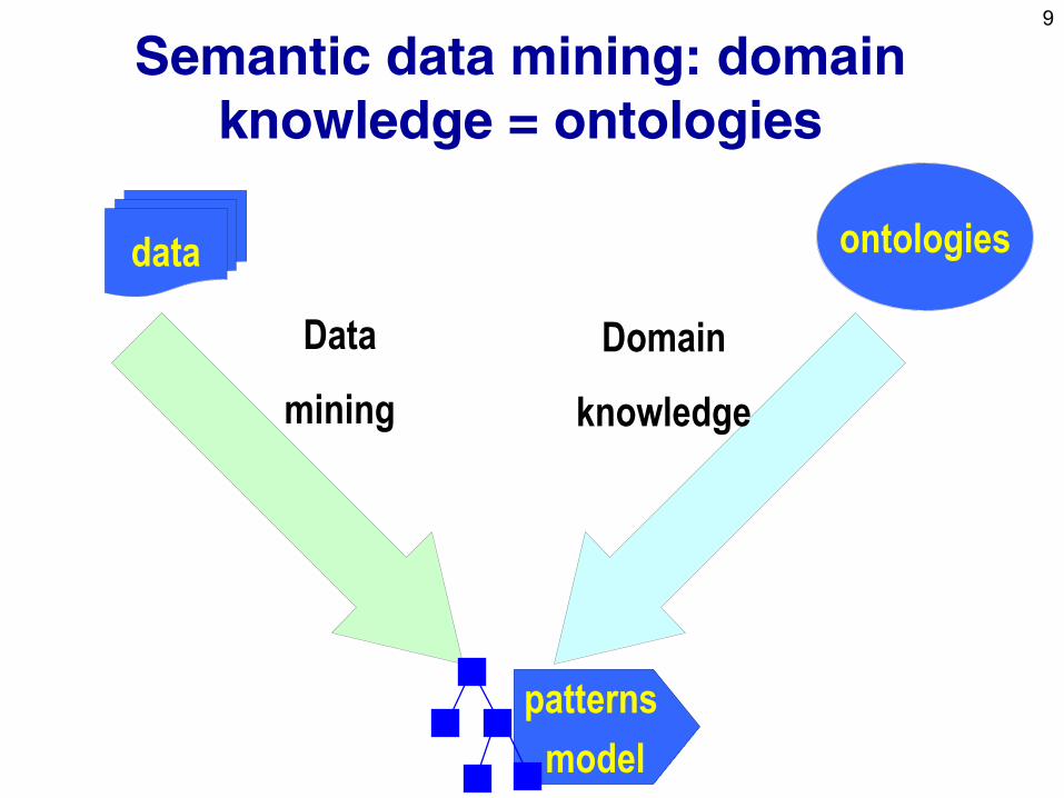
Semantic data mining: domain
knowledge = ontologies
Data
mining
Domain
knowledge
patterns
odel
patterns
model
data ontologies
10
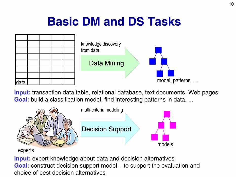
Basic DM and DS Tasks
data
Data MiningData Mining
knowledge discovery
from data
experts
Decision SupportDecision Support
mutli-criteria modeling
models
model, patterns, …
Input: transaction data table, relational database, text documents, Web pages
Goal: build a classification model, find interesting patterns in data, ...
Input: expert knowledge about data and decision alternatives
Goal: construct decision support model – to support the evaluation and
choice of best decision alternatives
11
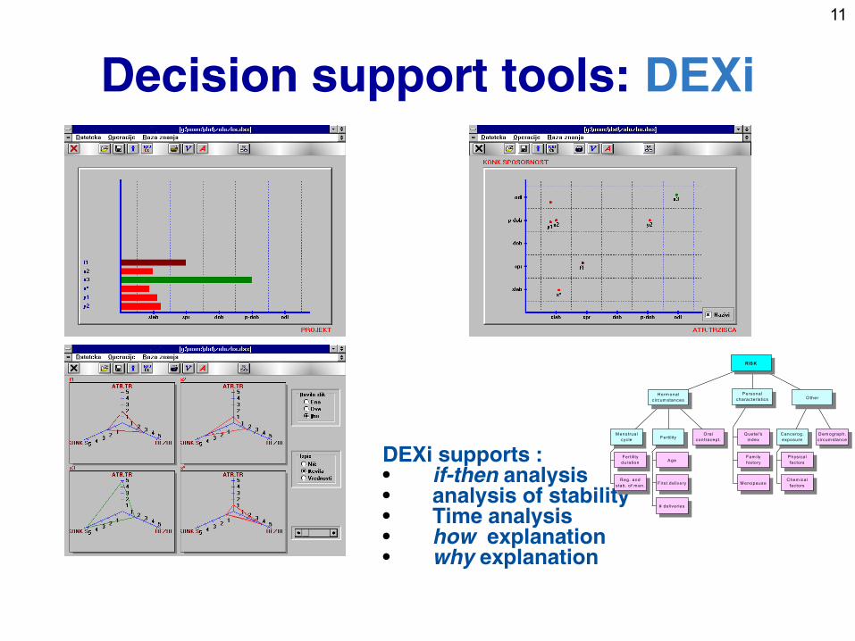
Decision support tools: DEXi
DEXi supports : • if-then analysis • analysis of stability • Time analysis • how explanation • why explanation
Horm onal
c ircum stances
Personal
characteris tics O ther
M enstrual
cyc leFertility
O ral
contracept.
RIS K
Cancerog.
exposure
Fertility
duration
Reg. and
stab. o f m en.
Age
Firs t de livery
# deliveries
Q uete l's
index
Fam ily
h is tory
Dem ograph.
c ircum stance
Phys ica l
factors
Chem ical
factorsM enopause
12
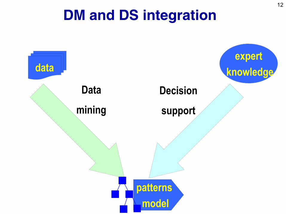
DM and DS integration
Data
mining
Decision
support
patterns
odel
patterns
model
data expert
knowledge
13
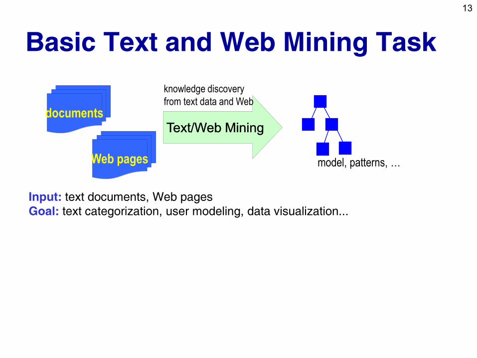
Basic Text and Web Mining Task
TextText//Web Web MiningMining
knowledge discovery
from text data and Web
model, patterns, …
Input: text documents, Web pages
Goal: text categorization, user modeling, data visualization...
documents
Web pages
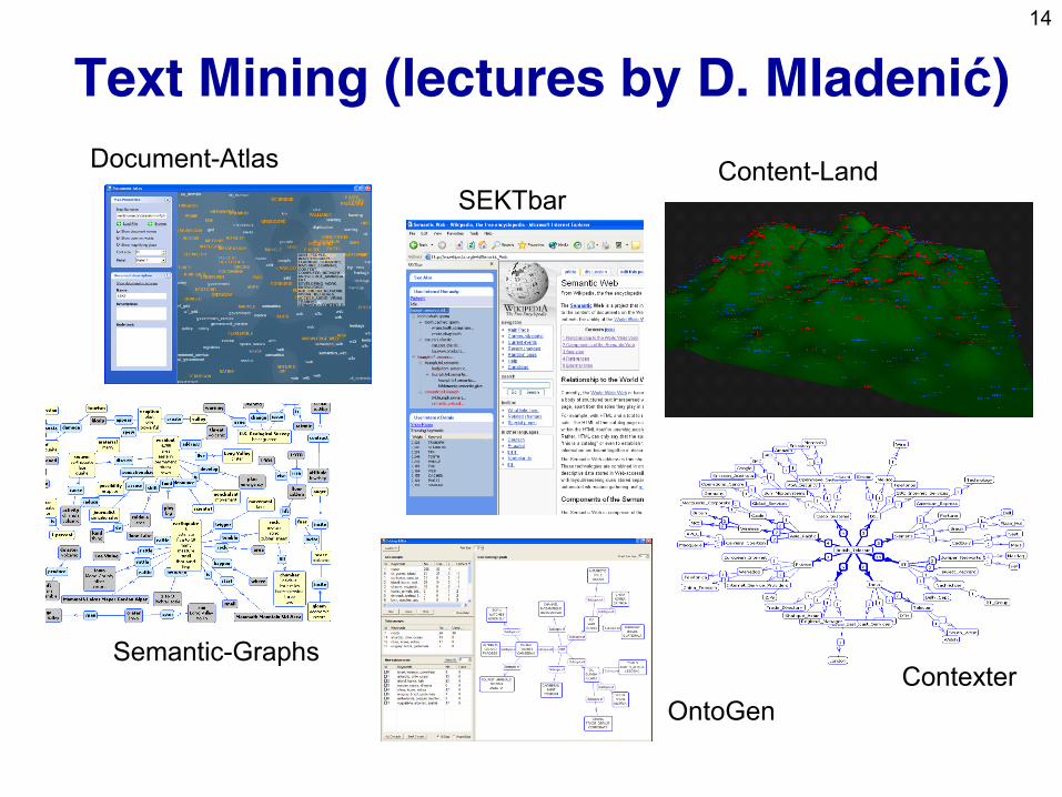
14
Text Mining (lectures by D. Mladenić)
SEKTbar
Document-Atlas
Contexter
OntoGen
Semantic-Graphs
Content-Land
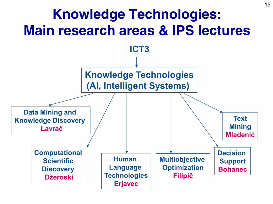
15
Knowledge Technologies:
Main research areas & IPS lectures
ICT3
Knowledge Technologies
(AI, Intelligent Systems)
Data Mining and
Knowledge Discovery
Lavrač
Computational
Scientific
Discovery
Džeroski
Human
Language
Technologies
Erjavec
Decision
Support
Bohanec
Text
Mining
Mladenić
Multiobjective
Optimization
Filipič

16
http//:videolectures.net
videolectures.net portal
~ 10,000 lectures
17
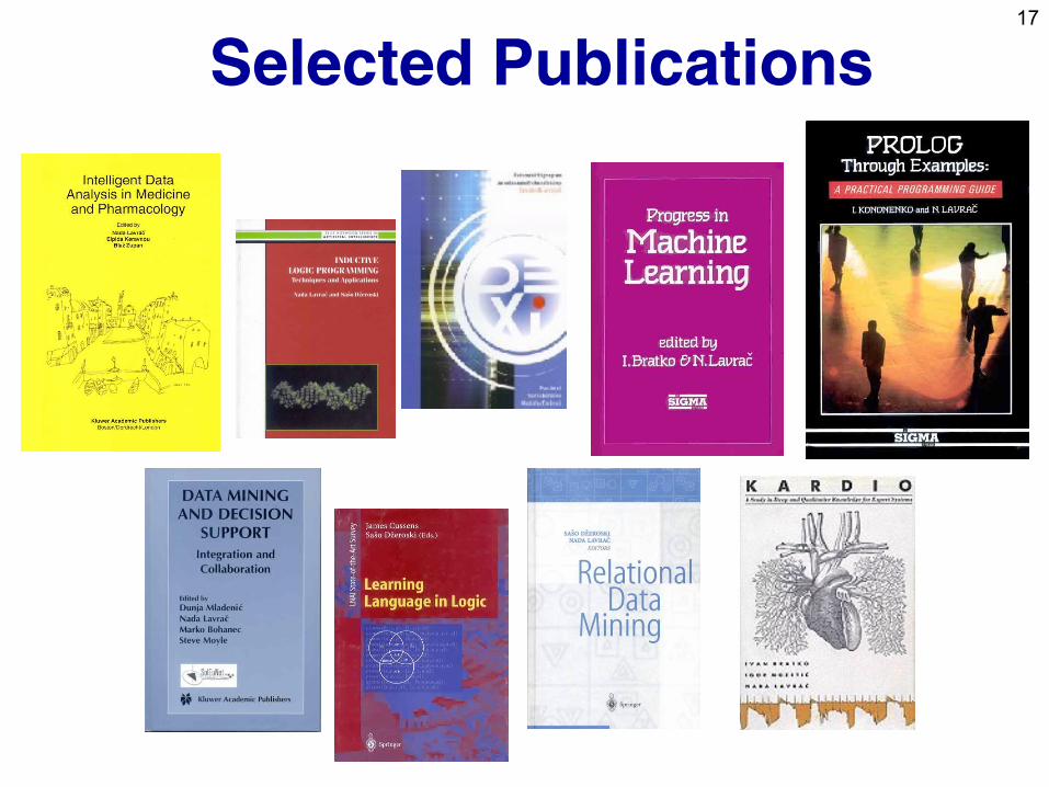
Selected Publications
18
Part I. Introduction
• Data Mining in a Nutshell
• Predictive and descriptive DM techniques
• Data Mining and the KDD process
• DM standards, tools and visualization
19
What is DM
• Extraction of useful information from data:
discovering relationships that have not
previously been known
• The viewpoint in this course: Data Mining is
the application of Machine Learning
techniques to solve real-life data analysis
problems
20
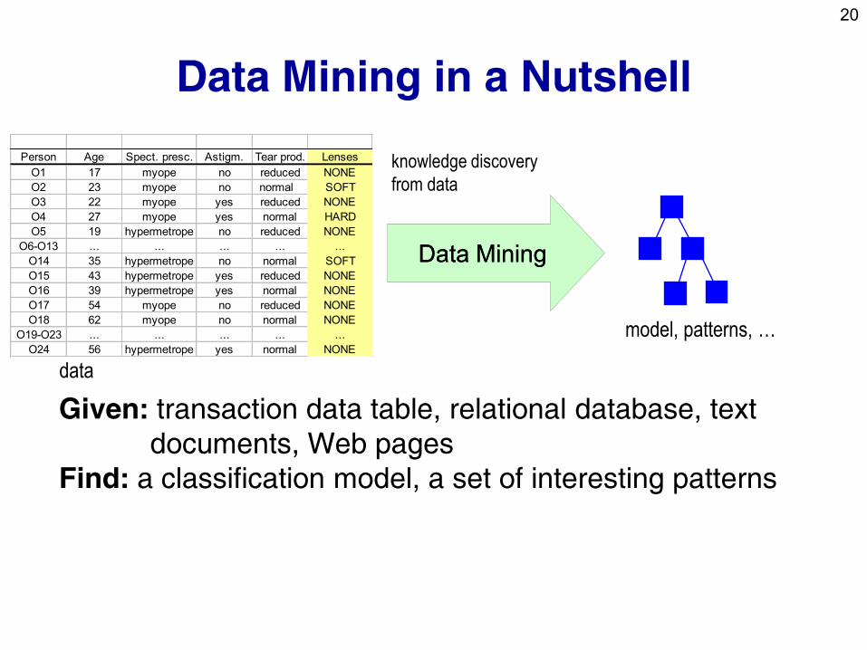
Data Mining in a Nutshell
data
Data MiningData Mining
knowledge discovery
from data
model, patterns, …
Given: transaction data table, relational database, text
documents, Web pages
Find: a classification model, a set of interesting patterns
Person Age Spect. presc. Astigm. Tear prod. Lenses
O1 17 myope no reduced NONE
O2 23 myope no normal SOFT
O3 22 myope yes reduced NONE
O4 27 myope yes normal HARD
O5 19 hypermetrope no reduced NONE
O6-O13 ... ... ... ... ...
O14 35 hypermetrope no normal SOFT
O15 43 hypermetrope yes reduced NONE
O16 39 hypermetrope yes normal NONE
O17 54 myope no reduced NONE
O18 62 myope no normal NONE
O19-O23 ... ... ... ... ...
O24 56 hypermetrope yes normal NONE
21
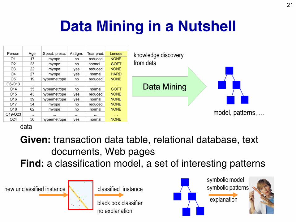
Data Mining in a Nutshell
data
Data MiningData Mining
knowledge discovery
from data
model, patterns, …
Given: transaction data table, relational database, text
documents, Web pages
Find: a classification model, a set of interesting patterns
new unclassified instance classified instance
black box classifier
no explanation
symbolic model
symbolic patterns
explanation
Person Age Spect. presc. Astigm. Tear prod. Lenses
O1 17 myope no reduced NONE
O2 23 myope no normal SOFT
O3 22 myope yes reduced NONE
O4 27 myope yes normal HARD
O5 19 hypermetrope no reduced NONE
O6-O13 ... ... ... ... ...
O14 35 hypermetrope no normal SOFT
O15 43 hypermetrope yes reduced NONE
O16 39 hypermetrope yes normal NONE
O17 54 myope no reduced NONE
O18 62 myope no normal NONE
O19-O23 ... ... ... ... ...
O24 56 hypermetrope yes normal NONE
22
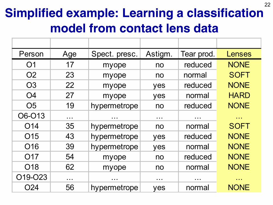
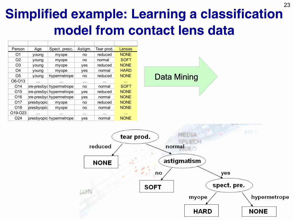
Simplified example: Learning a classification
model from contact lens data
Person Age Spect. presc. Astigm. Tear prod. Lenses
O1 17 myope no reduced NONE
O2 23 myope no normal SOFT
O3 22 myope yes reduced NONE
O4 27 myope yes normal HARD
O5 19 hypermetrope no reduced NONE
O6-O13 ... ... ... ... ...
O14 35 hypermetrope no normal SOFT
O15 43 hypermetrope yes reduced NONE
O16 39 hypermetrope yes normal NONE
O17 54 myope no reduced NONE
O18 62 myope no normal NONE
O19-O23 ... ... ... ... ...
O24 56 hypermetrope yes normal NONE
23
Simplified example: Learning a classification
model from contact lens data
Person Age Spect. presc. Astigm. Tear prod. Lenses
O1 young myope no reduced NONE
O2 young myope no normal SOFT
O3 young myope yes reduced NONE
O4 young myope yes normal HARD
O5 young hypermetrope no reduced NONE
O6-O13 ... ... ... ... ...
O14 pre-presbyohypermetrope no normal SOFT
O15 pre-presbyohypermetrope yes reduced NONE
O16 pre-presbyohypermetrope yes normal NONE
O17 presbyopic myope no reduced NONE
O18 presbyopic myope no normal NONE
O19-O23 ... ... ... ... ...
O24 presbyopic hypermetrope yes normal NONE
Data MiningData Mining
24
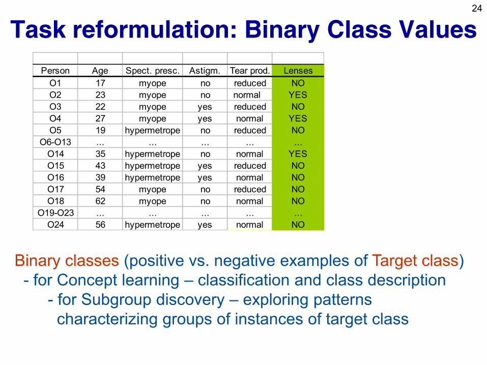
Task reformulation: Binary Class Values
Binary classes (positive vs. negative examples of Target class)
- for Concept learning – classification and class description
- for Subgroup discovery – exploring patterns
characterizing groups of instances of target class
Person Age Spect. presc. Astigm. Tear prod. Lenses
O1 17 myope no reduced NO
O2 23 myope no normal YES
O3 22 myope yes reduced NO
O4 27 myope yes normal YES
O5 19 hypermetrope no reduced NO
O6-O13 ... ... ... ... ...
O14 35 hypermetrope no normal YES
O15 43 hypermetrope yes reduced NO
O16 39 hypermetrope yes normal NO
O17 54 myope no reduced NO
O18 62 myope no normal NO
O19-O23 ... ... ... ... ...
O24 56 hypermetrope yes normal NO
25
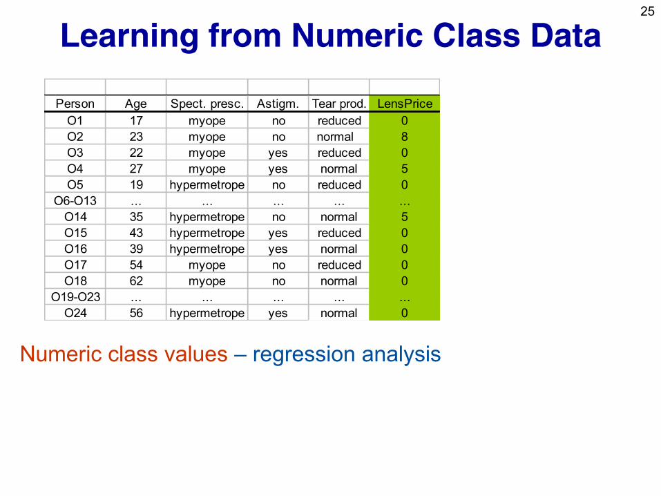
Learning from Numeric Class Data
Numeric class values – regression analysis
Person Age Spect. presc. Astigm. Tear prod. LensPrice
O1 17 myope no reduced 0
O2 23 myope no normal 8
O3 22 myope yes reduced 0
O4 27 myope yes normal 5
O5 19 hypermetrope no reduced 0
O6-O13 ... ... ... ... ...
O14 35 hypermetrope no normal 5
O15 43 hypermetrope yes reduced 0
O16 39 hypermetrope yes normal 0
O17 54 myope no reduced 0
O18 62 myope no normal 0
O19-O23 ... ... ... ... ...
O24 56 hypermetrope yes normal 0
26
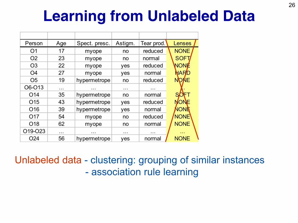
Learning from Unlabeled Data
Unlabeled data - clustering: grouping of similar instances
- association rule learning
Person Age Spect. presc. Astigm. Tear prod. Lenses
O1 17 myope no reduced NONE
O2 23 myope no normal SOFT
O3 22 myope yes reduced NONE
O4 27 myope yes normal HARD
O5 19 hypermetrope no reduced NONE
O6-O13 ... ... ... ... ...
O14 35 hypermetrope no normal SOFT
O15 43 hypermetrope yes reduced NONE
O16 39 hypermetrope yes normal NONE
O17 54 myope no reduced NONE
O18 62 myope no normal NONE
O19-O23 ... ... ... ... ...
O24 56 hypermetrope yes normal NONE
27
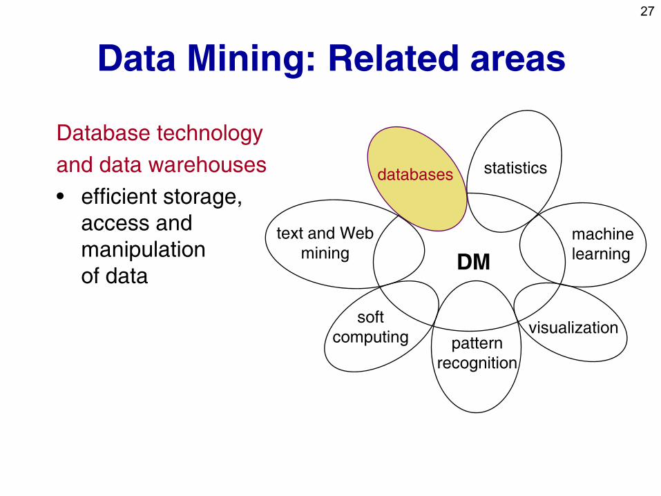
Data Mining: Related areas
Database technology
and data warehouses
• efficient storage,
access and
manipulation
of data DM
statistics
machine
learning
visualization
text and Web
mining
soft
computing pattern
recognition
databases
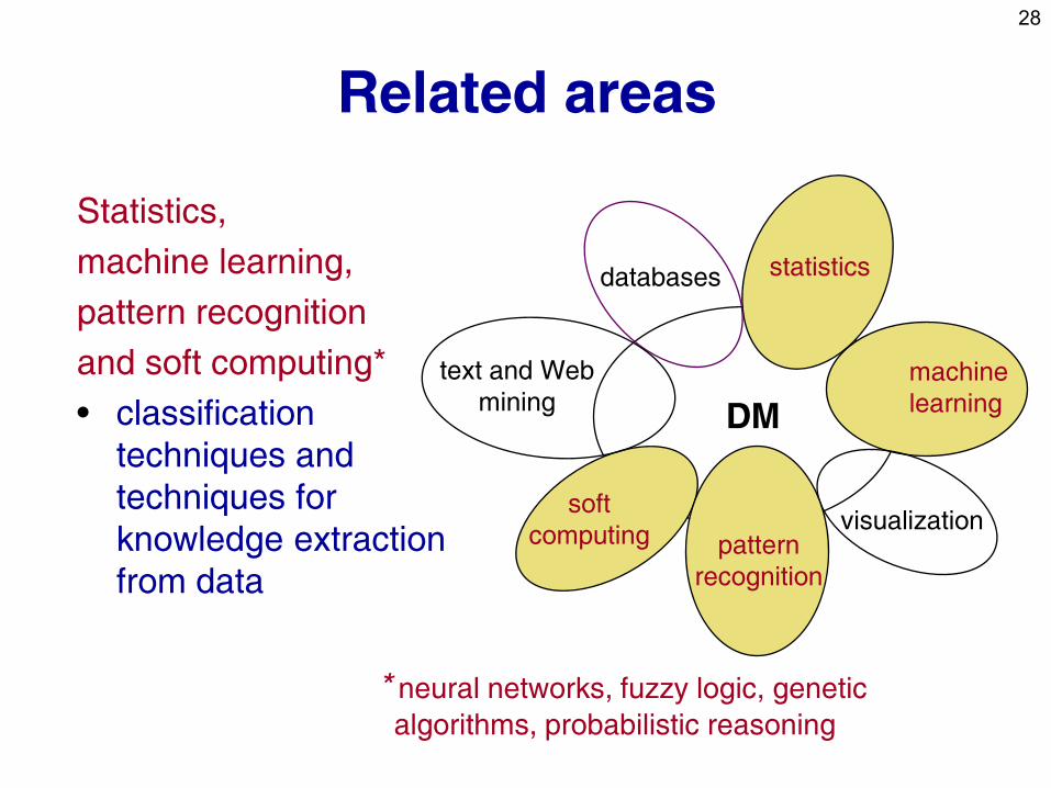
28
Statistics,
machine learning,
pattern recognition
and soft computing*
• classification
techniques and
techniques for
knowledge extraction
from data
* neural networks, fuzzy logic, genetic
algorithms, probabilistic reasoning
DM
statistics
machine
learning
visualization
text and Web
mining
soft
computing pattern
recognition
databases
Related areas
29
DM
statistics
machine
learning
visualization
text and Web
mining
soft
computing pattern
recognition
databases
Related areas
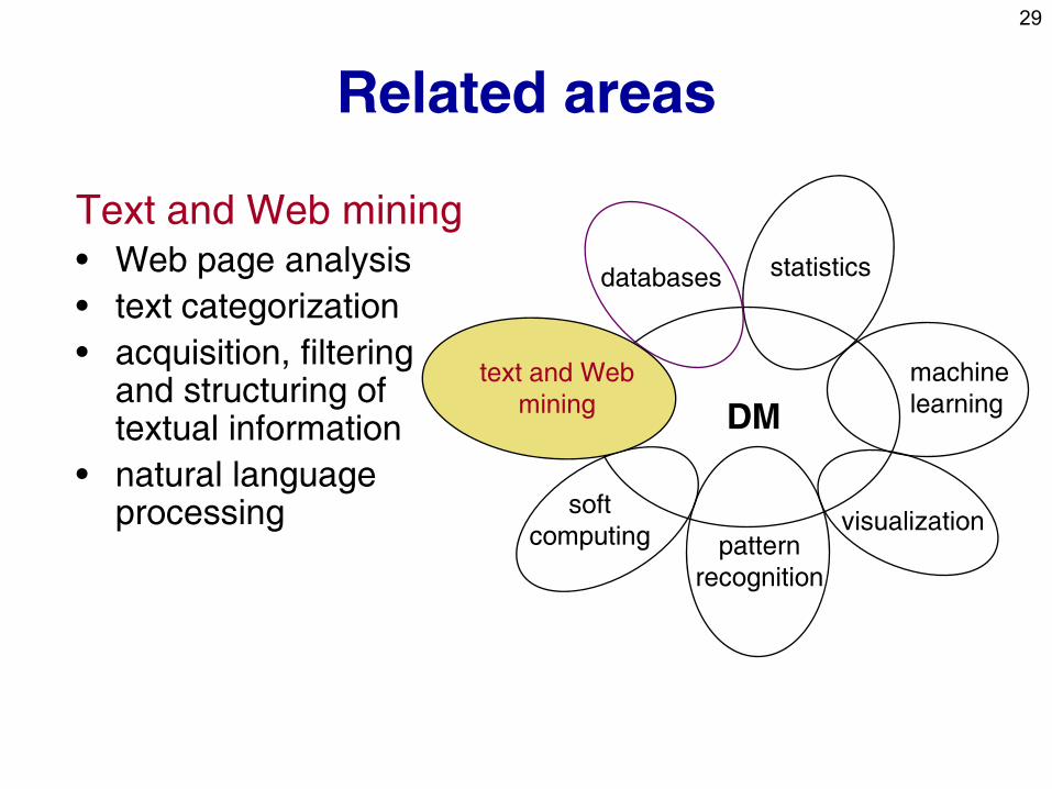
Text and Web mining • Web page analysis
• text categorization
• acquisition, filtering and structuring of textual information
• natural language processing
text and Web
mining
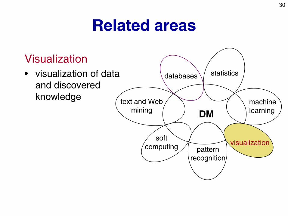
30
Related areas
Visualization
• visualization of data
and discovered
knowledge
DM
statistics
machine
learning
visualization
text and Web
mining
soft
computing pattern
recognition
databases
31
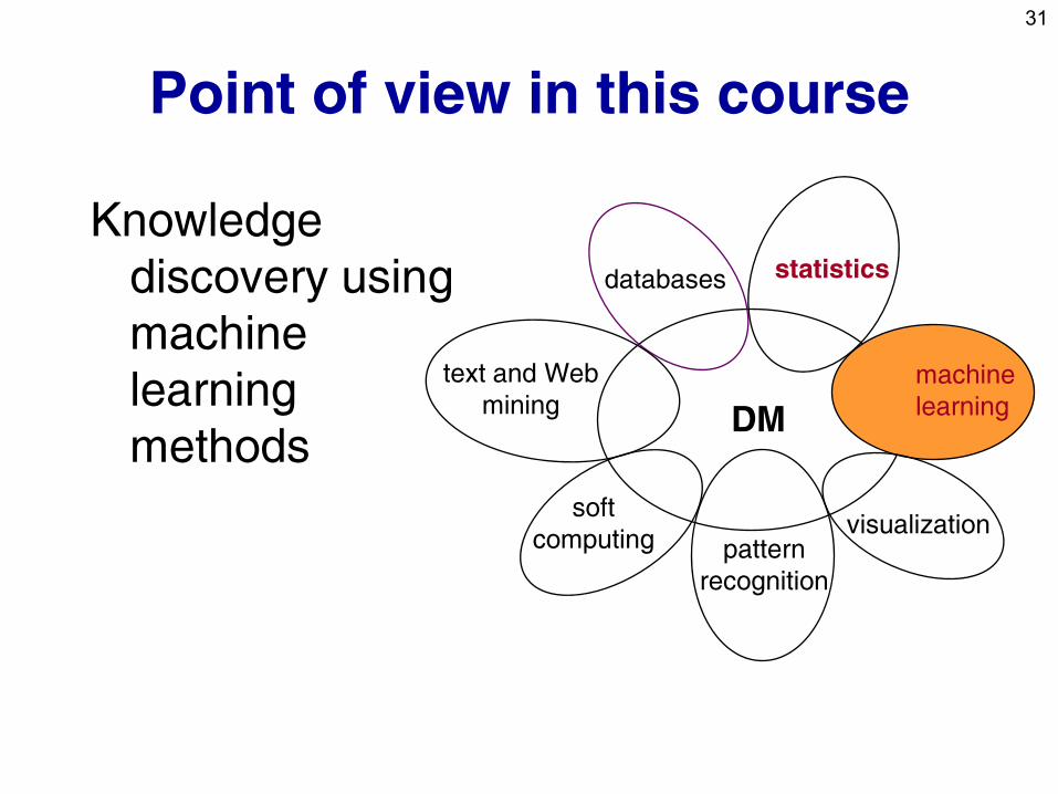
Point of view in this course
Knowledge
discovery using
machine
learning
methods
DM
statistics
machine
learning
visualization
text and Web
mining
soft
computing pattern
recognition
databases
32
Data Mining, ML and Statistics
• All three areas have a long tradition of developing inductive techniques for data analysis.
– reasoning from properties of a data sample to properties of a population
• DM vs. ML - Viewpoint in this course:
– Data Mining is the application of Machine Learning techniques to hard real-life data analysis problems
33
Data Mining, ML and Statistics
• All three areas have a long tradition of developing inductive techniques for data analysis.
– reasoning from properties of a data sample to properties of a population
• DM vs. Statistics:
– Statistics
• Hypothesis testing when certain theoretical expectations about the data distribution, independence, random sampling, sample size, etc. are satisfied
• Main approach: best fitting all the available data
– Data mining
• Automated construction of understandable patterns, and structured models
• Main approach: structuring the data space, heuristic search for decision trees, rules, … covering (parts of) the data space
34
Part I. Introduction
• Data Mining in a Nutshell
• Predictive and descriptive DM techniques
• Data Mining and the KDD process
• DM standards, tools and visualization
35
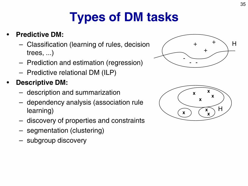
Types of DM tasks • Predictive DM:
– Classification (learning of rules, decision
trees, ...)
– Prediction and estimation (regression)
– Predictive relational DM (ILP)
• Descriptive DM:
– description and summarization
– dependency analysis (association rule
learning)
– discovery of properties and constraints
– segmentation (clustering)
– subgroup discovery
+ +
+
- - -
H
x x
x x
+ x x x
H
36
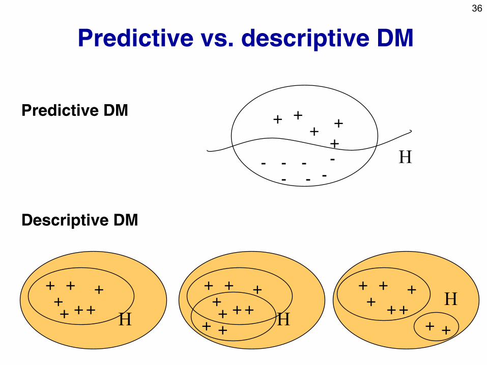
Predictive vs. descriptive DM
Predictive DM
Descriptive DM
+
-
+ +
+
+
- -
- - -
- H
+ + + +
+ + +
H + +
+ + +
+ + +
H + +
+
+ + + +
+ + + H
+ +
37
Predictive vs. descriptive DM
• Predictive DM: Inducing classifiers for solving
classification and prediction tasks,
– Classification rule learning, Decision tree learning, ...
– Bayesian classifier, ANN, SVM, ...
– Data analysis through hypothesis generation and testing
• Descriptive DM: Discovering interesting regularities in
the data, uncovering patterns, ... for solving KDD tasks
– Symbolic clustering, Association rule learning, Subgroup
discovery, ...
– Exploratory data analysis
38
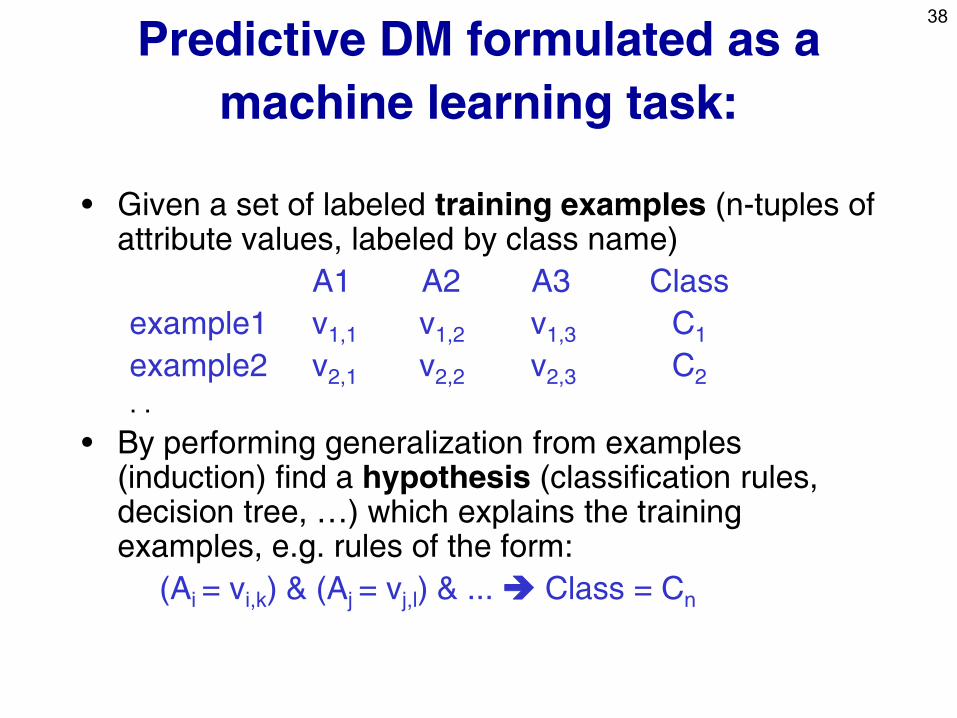
Predictive DM formulated as a
machine learning task:
• Given a set of labeled training examples (n-tuples of attribute values, labeled by class name)
A1 A2 A3 Class
example1 v1,1 v1,2 v1,3 C1
example2 v2,1 v2,2 v2,3 C2
. .
• By performing generalization from examples (induction) find a hypothesis (classification rules, decision tree, …) which explains the training examples, e.g. rules of the form:
(Ai = vi,k) & (Aj = vj,l) & ... Class = Cn
39
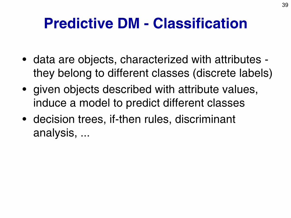
Predictive DM - Classification
• data are objects, characterized with attributes -
they belong to different classes (discrete labels)
• given objects described with attribute values,
induce a model to predict different classes
• decision trees, if-then rules, discriminant
analysis, ...
40
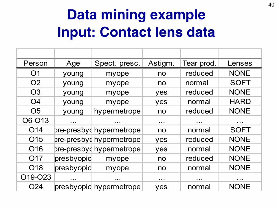
Data mining example
Input: Contact lens data
Person Age Spect. presc. Astigm. Tear prod. Lenses
O1 young myope no reduced NONE
O2 young myope no normal SOFT
O3 young myope yes reduced NONE
O4 young myope yes normal HARD
O5 young hypermetrope no reduced NONE
O6-O13 ... ... ... ... ...
O14 pre-presbyohypermetrope no normal SOFT
O15 pre-presbyohypermetrope yes reduced NONE
O16 pre-presbyohypermetrope yes normal NONE
O17 presbyopic myope no reduced NONE
O18 presbyopic myope no normal NONE
O19-O23 ... ... ... ... ...
O24 presbyopic hypermetrope yes normal NONE
41
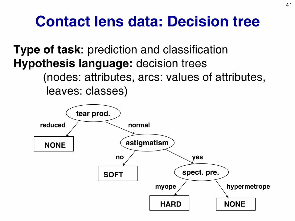
Contact lens data: Decision tree
tear prod.
astigmatism
spect. pre.
NONE
NONE
reduced
no yes
normal
hypermetrope
SOFT
myope
HARD
Type of task: prediction and classification
Hypothesis language: decision trees
(nodes: attributes, arcs: values of attributes,
leaves: classes)
42
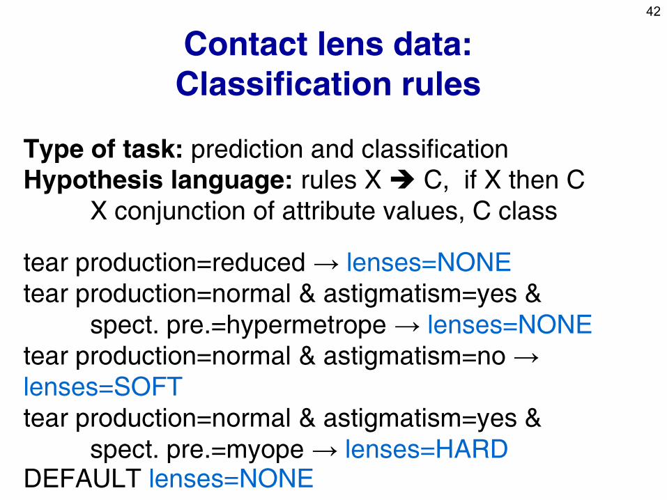
Contact lens data:
Classification rules
Type of task: prediction and classification
Hypothesis language: rules X C, if X then C X conjunction of attribute values, C class
tear production=reduced → lenses=NONE
tear production=normal & astigmatism=yes &
spect. pre.=hypermetrope → lenses=NONE
tear production=normal & astigmatism=no →
lenses=SOFT
tear production=normal & astigmatism=yes &
spect. pre.=myope → lenses=HARD DEFAULT lenses=NONE
43
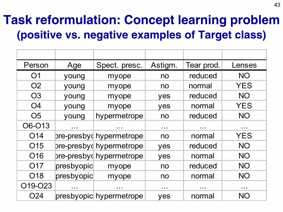
Task reformulation: Concept learning problem (positive vs. negative examples of Target class)
Person Age Spect. presc. Astigm. Tear prod. Lenses
O1 young myope no reduced NO
O2 young myope no normal YES
O3 young myope yes reduced NO
O4 young myope yes normal YES
O5 young hypermetrope no reduced NO
O6-O13 ... ... ... ... ...
O14 pre-presbyohypermetrope no normal YES
O15 pre-presbyohypermetrope yes reduced NO
O16 pre-presbyohypermetrope yes normal NO
O17 presbyopic myope no reduced NO
O18 presbyopic myope no normal NO
O19-O23 ... ... ... ... ...
O24 presbyopic hypermetrope yes normal NO
44
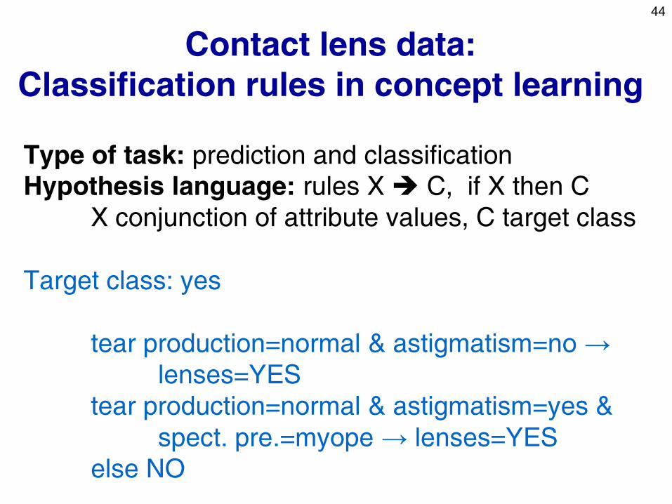
Contact lens data:
Classification rules in concept learning
Type of task: prediction and classification
Hypothesis language: rules X C, if X then C X conjunction of attribute values, C target class
Target class: yes
tear production=normal & astigmatism=no →
lenses=YES
tear production=normal & astigmatism=yes &
spect. pre.=myope → lenses=YES
else NO
45
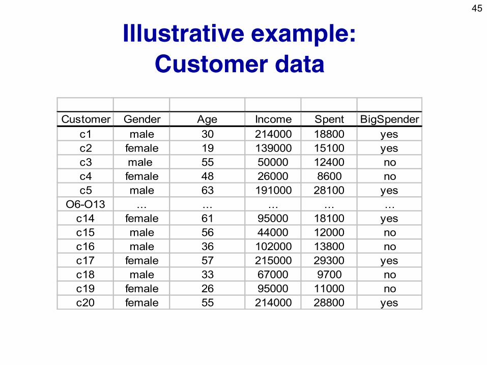
Illustrative example:
Customer data
Customer Gender Age Income Spent BigSpender
c1 male 30 214000 18800 yes
c2 female 19 139000 15100 yes
c3 male 55 50000 12400 no
c4 female 48 26000 8600 no
c5 male 63 191000 28100 yes
O6-O13 ... ... ... ... ...
c14 female 61 95000 18100 yes
c15 male 56 44000 12000 no
c16 male 36 102000 13800 no
c17 female 57 215000 29300 yes
c18 male 33 67000 9700 no
c19 female 26 95000 11000 no
c20 female 55 214000 28800 yes
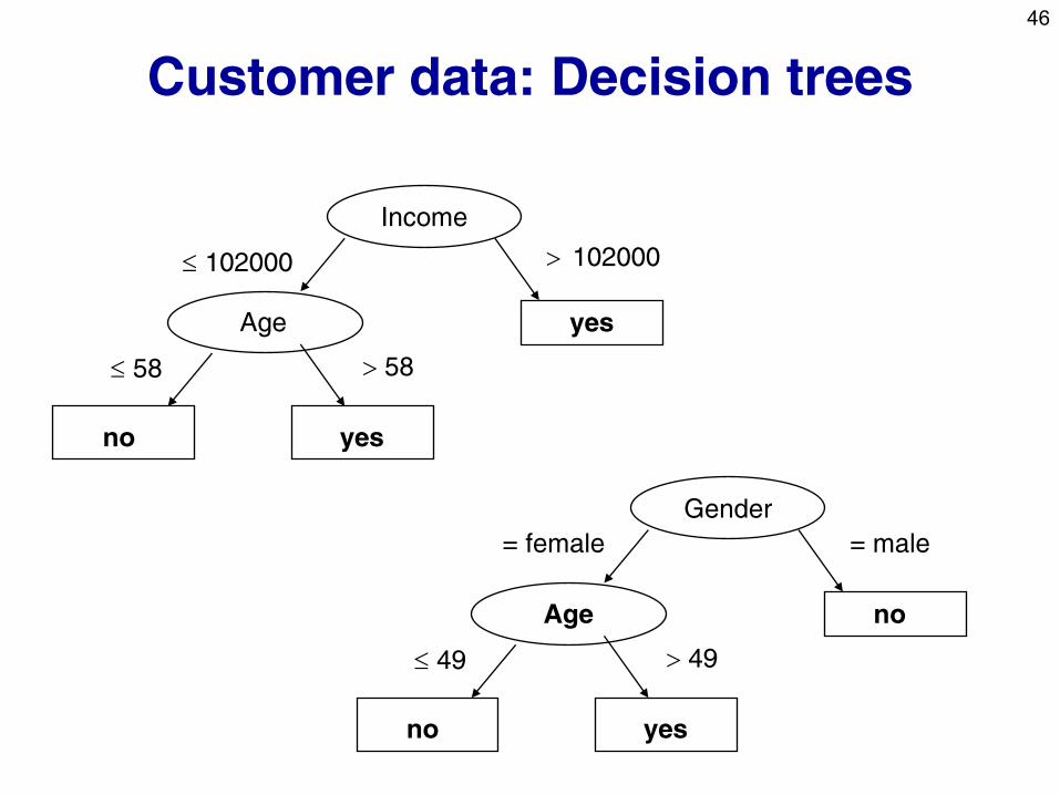
46
Customer data: Decision trees
Income
Age
no
yes
102000 102000
58 58
yes
Gender
Age
no
no
= female = male
49 49
yes
47
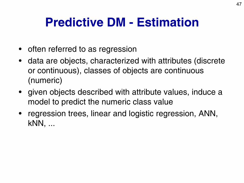
Predictive DM - Estimation
• often referred to as regression
• data are objects, characterized with attributes (discrete
or continuous), classes of objects are continuous
(numeric)
• given objects described with attribute values, induce a
model to predict the numeric class value
• regression trees, linear and logistic regression, ANN,
kNN, ...
48
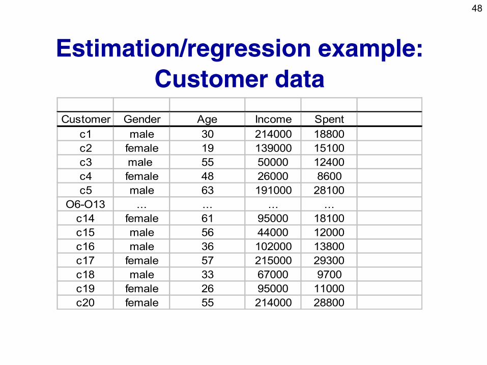
Estimation/regression example:
Customer data
Customer Gender Age Income Spent
c1 male 30 214000 18800
c2 female 19 139000 15100
c3 male 55 50000 12400
c4 female 48 26000 8600
c5 male 63 191000 28100
O6-O13 ... ... ... ...
c14 female 61 95000 18100
c15 male 56 44000 12000
c16 male 36 102000 13800
c17 female 57 215000 29300
c18 male 33 67000 9700
c19 female 26 95000 11000
c20 female 55 214000 28800
49
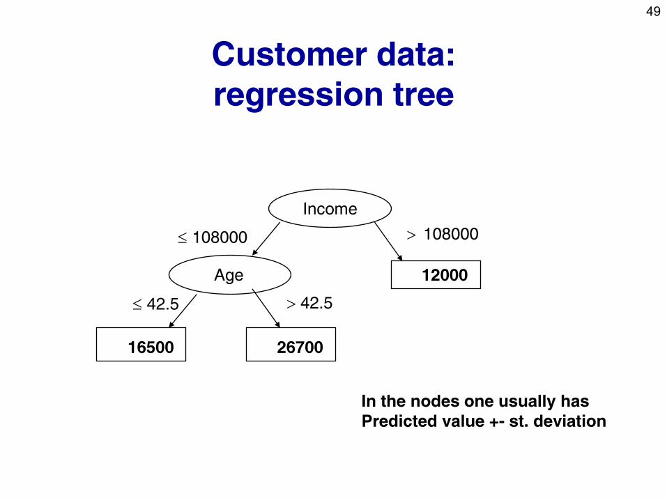
Customer data:
regression tree
Income
Age
16500
12000
108000 108000
42.5 42.5
26700
In the nodes one usually has
Predicted value +- st. deviation
50
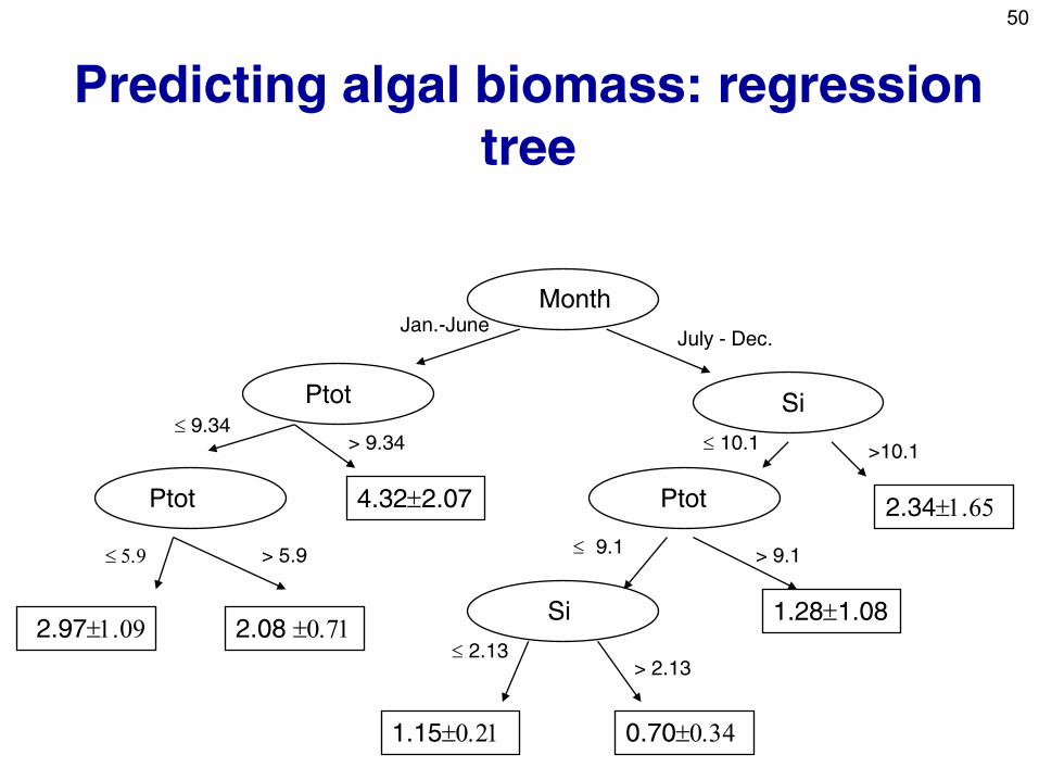
Predicting algal biomass: regression
tree
Month
Ptot
2.341.65 Ptot
Si
Si 2.08 0.71 2.971.09
Ptot 4.322.07
0.700.34 1.150.21
1.281.08
Jan.-June
> 9.34 10.1 >10.1
July - Dec.
> 2.13 2.13
9.1 > 9.1
9.34
5.9 > 5.9
51
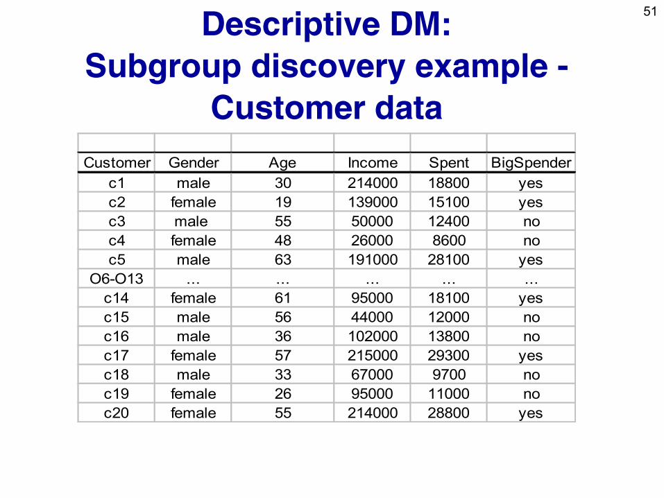
Descriptive DM:
Subgroup discovery example -
Customer data
Customer Gender Age Income Spent BigSpender
c1 male 30 214000 18800 yes
c2 female 19 139000 15100 yes
c3 male 55 50000 12400 no
c4 female 48 26000 8600 no
c5 male 63 191000 28100 yes
O6-O13 ... ... ... ... ...
c14 female 61 95000 18100 yes
c15 male 56 44000 12000 no
c16 male 36 102000 13800 no
c17 female 57 215000 29300 yes
c18 male 33 67000 9700 no
c19 female 26 95000 11000 no
c20 female 55 214000 28800 yes
52
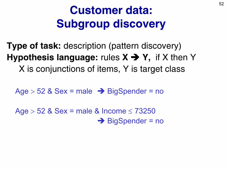
Customer data:
Subgroup discovery
Type of task: description (pattern discovery)
Hypothesis language: rules X Y, if X then Y
X is conjunctions of items, Y is target class
Age 52 & Sex = male BigSpender = no
Age 52 & Sex = male & Income 73250
BigSpender = no
53
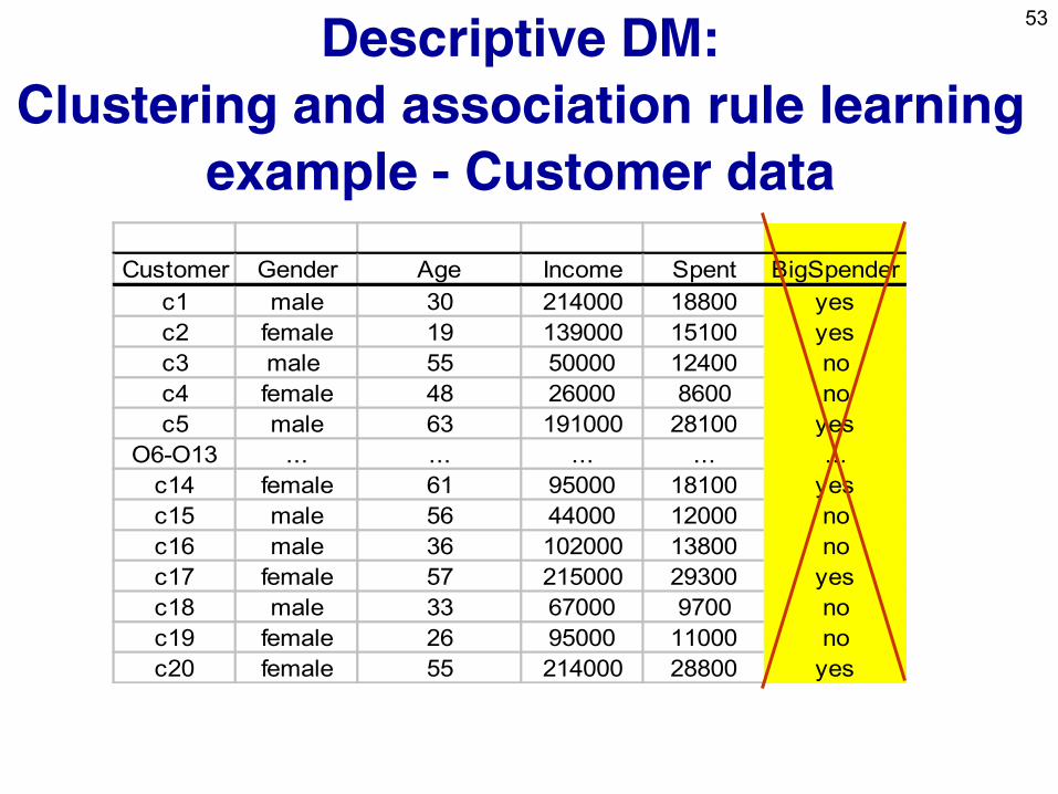
Descriptive DM:
Clustering and association rule learning
example - Customer data
Customer Gender Age Income Spent BigSpender
c1 male 30 214000 18800 yes
c2 female 19 139000 15100 yes
c3 male 55 50000 12400 no
c4 female 48 26000 8600 no
c5 male 63 191000 28100 yes
O6-O13 ... ... ... ... ...
c14 female 61 95000 18100 yes
c15 male 56 44000 12000 no
c16 male 36 102000 13800 no
c17 female 57 215000 29300 yes
c18 male 33 67000 9700 no
c19 female 26 95000 11000 no
c20 female 55 214000 28800 yes
54
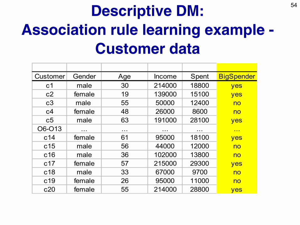
Descriptive DM:
Association rule learning example -
Customer data
Customer Gender Age Income Spent BigSpender
c1 male 30 214000 18800 yes
c2 female 19 139000 15100 yes
c3 male 55 50000 12400 no
c4 female 48 26000 8600 no
c5 male 63 191000 28100 yes
O6-O13 ... ... ... ... ...
c14 female 61 95000 18100 yes
c15 male 56 44000 12000 no
c16 male 36 102000 13800 no
c17 female 57 215000 29300 yes
c18 male 33 67000 9700 no
c19 female 26 95000 11000 no
c20 female 55 214000 28800 yes
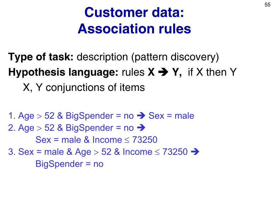
55
Customer data:
Association rules
Type of task: description (pattern discovery)
Hypothesis language: rules X Y, if X then Y
X, Y conjunctions of items
1. Age 52 & BigSpender = no Sex = male
2. Age 52 & BigSpender = no
Sex = male & Income 73250
3. Sex = male & Age 52 & Income 73250
BigSpender = no
56
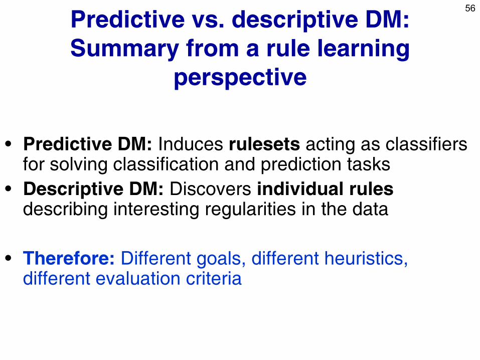
Predictive vs. descriptive DM:
Summary from a rule learning
perspective
• Predictive DM: Induces rulesets acting as classifiers for solving classification and prediction tasks
• Descriptive DM: Discovers individual rules describing interesting regularities in the data
• Therefore: Different goals, different heuristics, different evaluation criteria
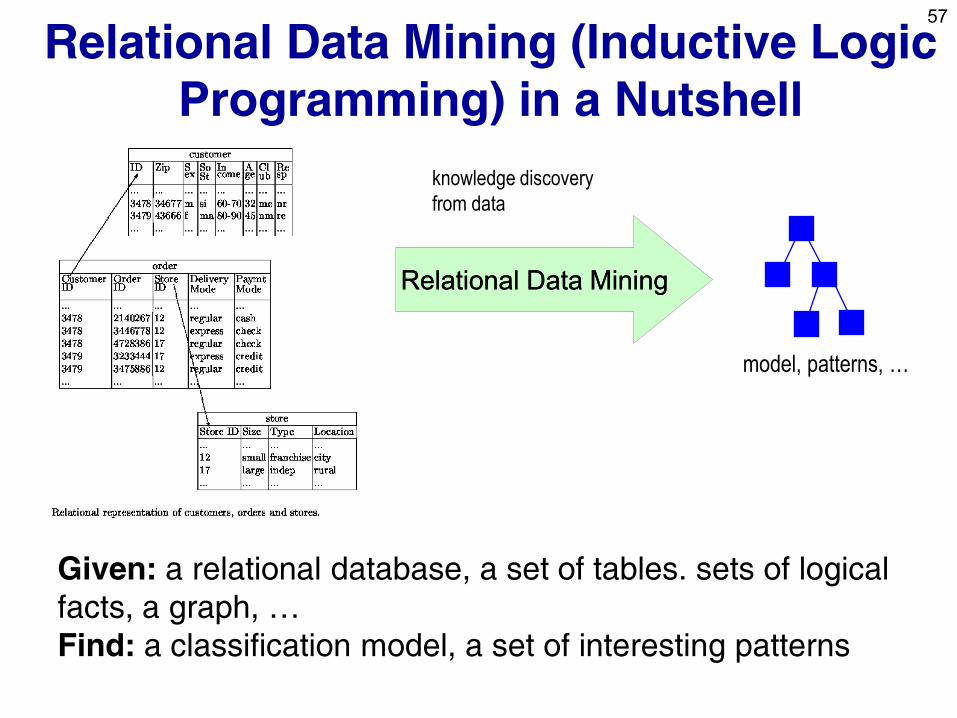
57
Relational Data Mining (Inductive Logic
Programming) in a Nutshell
Relational Relational Data MiningData Mining
knowledge discovery
from data
model, patterns, …
Given: a relational database, a set of tables. sets of logical
facts, a graph, …
Find: a classification model, a set of interesting patterns
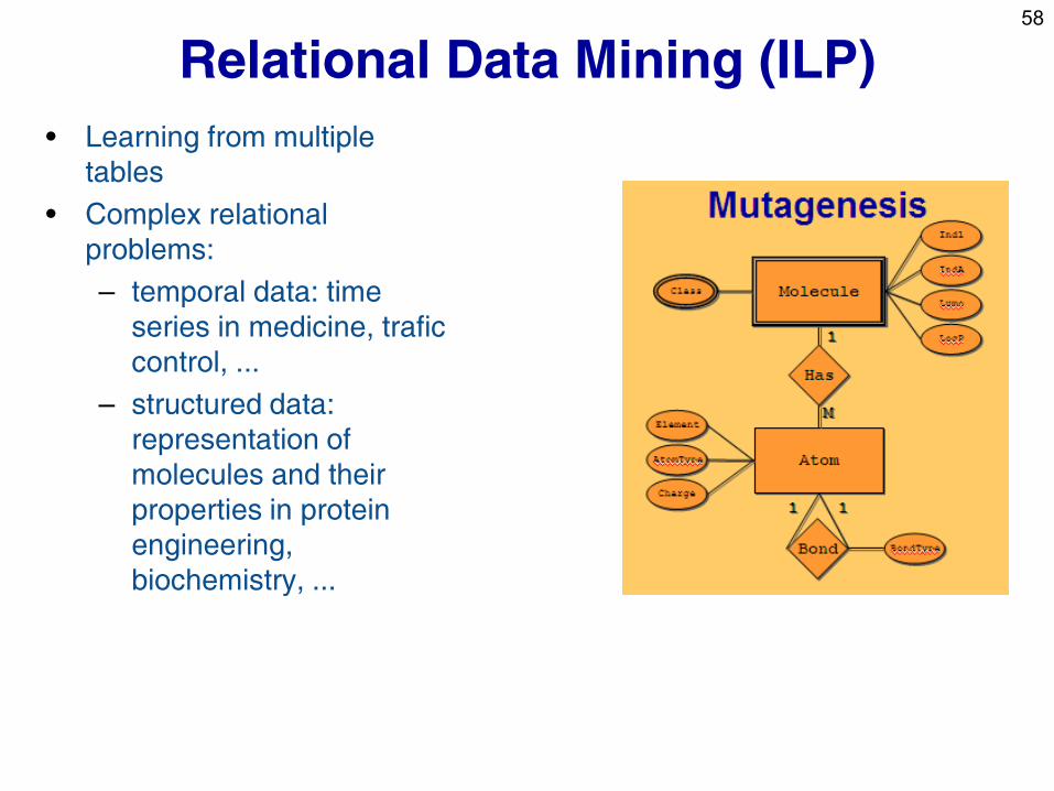
58
Relational Data Mining (ILP)
• Learning from multiple
tables
• Complex relational
problems:
– temporal data: time
series in medicine, trafic
control, ...
– structured data:
representation of
molecules and their
properties in protein
engineering,
biochemistry, ...
59
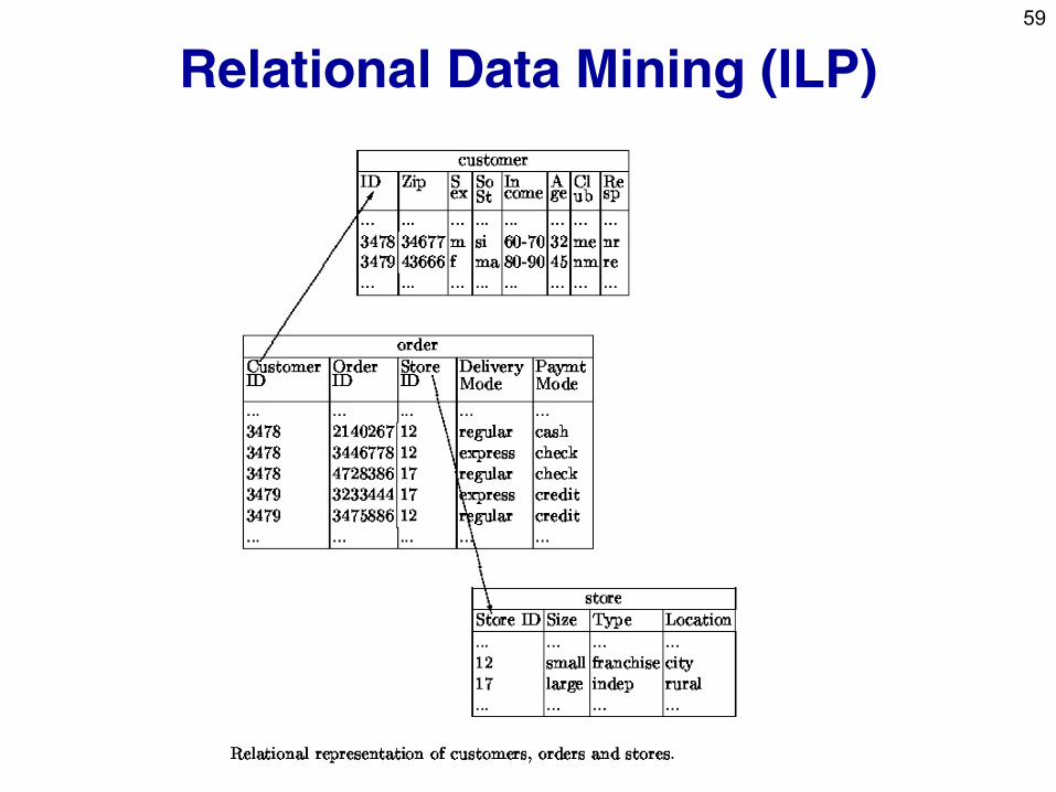
Relational Data Mining (ILP)
60
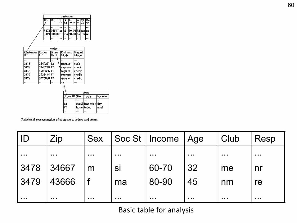
ID Zip Sex Soc St Income Age Club Resp
... ... ... ... ... ... ... ...
3478 34667 m si 60-70 32 me nr
3479 43666 f ma 80-90 45 nm re
... ... ... ... ... ... ... ...
Basic table for analysis
61
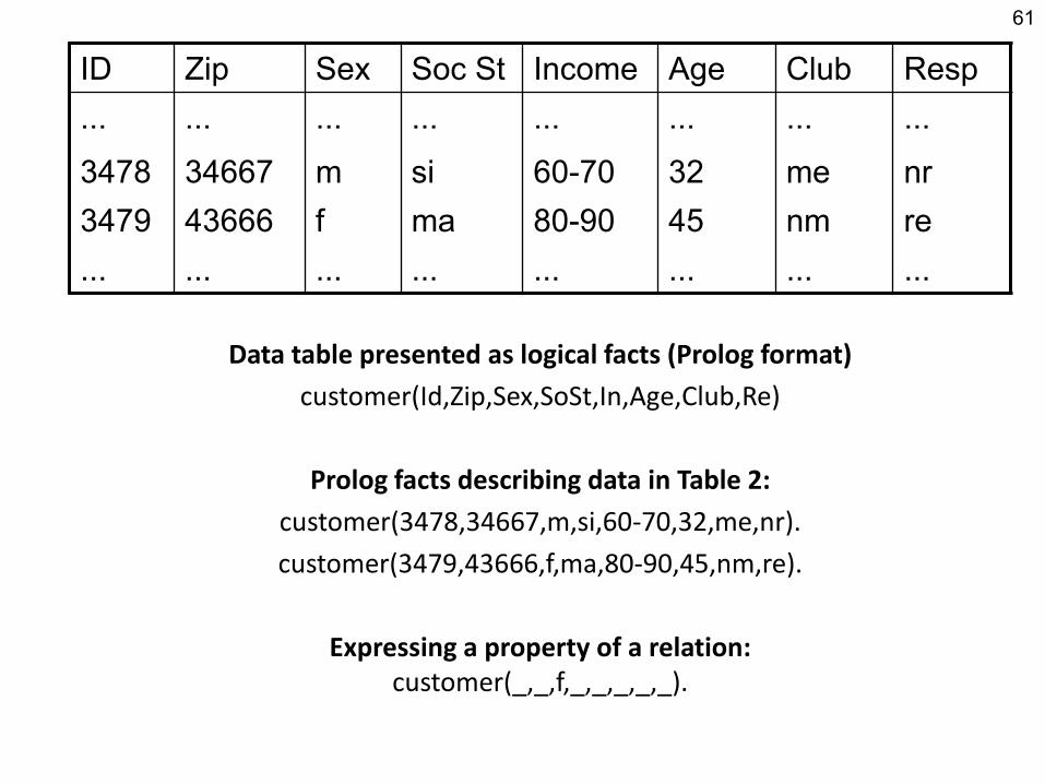
ID Zip Sex Soc St Income Age Club Resp
... ... ... ... ... ... ... ...
3478 34667 m si 60-70 32 me nr
3479 43666 f ma 80-90 45 nm re
... ... ... ... ... ... ... ...
Data table presented as logical facts (Prolog format)
customer(Id,Zip,Sex,SoSt,In,Age,Club,Re)
Prolog facts describing data in Table 2:
customer(3478,34667,m,si,60-70,32,me,nr).
customer(3479,43666,f,ma,80-90,45,nm,re).
Expressing a property of a relation: customer(_,_,f,_,_,_,_,_).
62
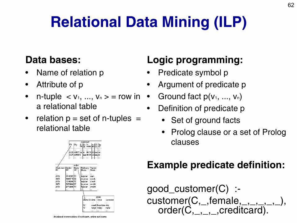
Relational Data Mining (ILP)
Logic programming:
• Predicate symbol p
• Argument of predicate p
• Ground fact p(v1, ..., vn)
• Definition of predicate p
• Set of ground facts
• Prolog clause or a set of Prolog
clauses
Example predicate definition:
good_customer(C) :-
customer(C,_,female,_,_,_,_,_), order(C,_,_,_,creditcard).
Data bases:
• Name of relation p
• Attribute of p
• n-tuple < v1, ..., vn > = row in
a relational table
• relation p = set of n-tuples =
relational table
63
Part I. Introduction
• Data Mining in a Nutshell
• Predictive and descriptive DM techniques
• Data Mining and the KDD process
• DM standards, tools and visualization
64
Data Mining and KDD
• KDD is defined as “the process of identifying valid, novel, potentially useful and ultimately understandable models/patterns in data.” *
• Data Mining (DM) is the key step in the KDD process, performed by using data mining techniques for extracting models or interesting patterns from the data.
Usama M. Fayyad, Gregory Piatesky-Shapiro, Pedhraic Smyth: The KDD Process for Extracting
Useful Knowledge form Volumes of Data. Comm ACM, Nov 96/Vol 39 No 11
65
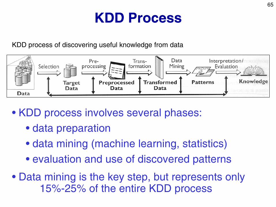
KDD Process
KDD process of discovering useful knowledge from data
• KDD process involves several phases:
• data preparation
• data mining (machine learning, statistics)
• evaluation and use of discovered patterns
• Data mining is the key step, but represents only 15%-25% of the entire KDD process
66
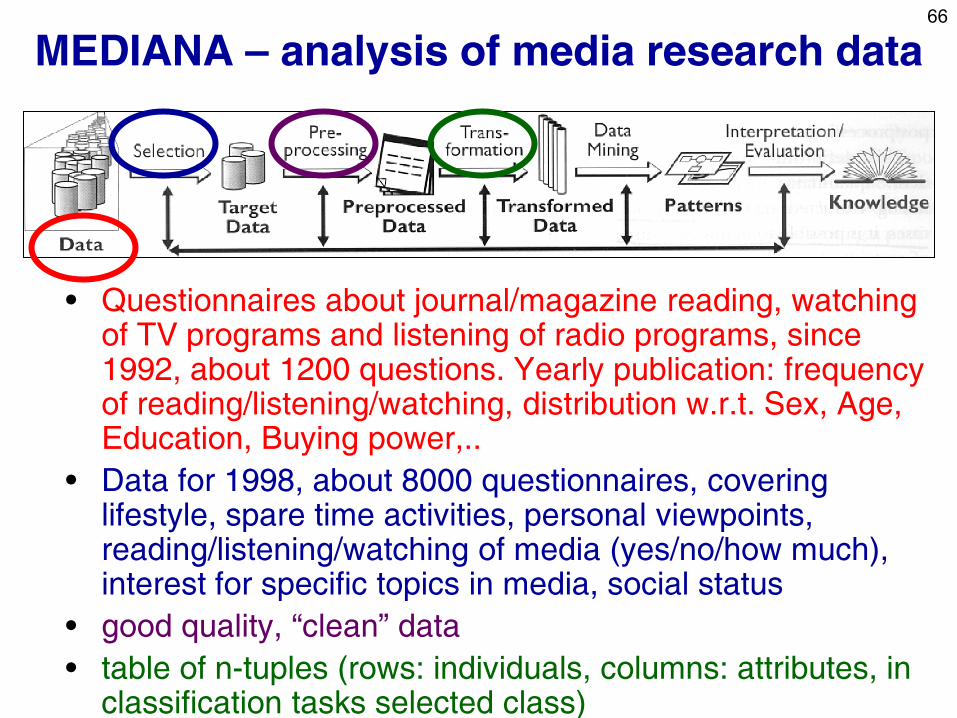
MEDIANA – analysis of media research data
• Questionnaires about journal/magazine reading, watching of TV programs and listening of radio programs, since 1992, about 1200 questions. Yearly publication: frequency of reading/listening/watching, distribution w.r.t. Sex, Age, Education, Buying power,..
• Data for 1998, about 8000 questionnaires, covering lifestyle, spare time activities, personal viewpoints, reading/listening/watching of media (yes/no/how much), interest for specific topics in media, social status
• good quality, “clean” data
• table of n-tuples (rows: individuals, columns: attributes, in classification tasks selected class)
67
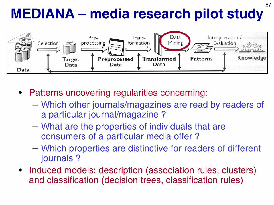
MEDIANA – media research pilot study
• Patterns uncovering regularities concerning:
– Which other journals/magazines are read by readers of a particular journal/magazine ?
– What are the properties of individuals that are consumers of a particular media offer ?
– Which properties are distinctive for readers of different journals ?
• Induced models: description (association rules, clusters) and classification (decision trees, classification rules)
68
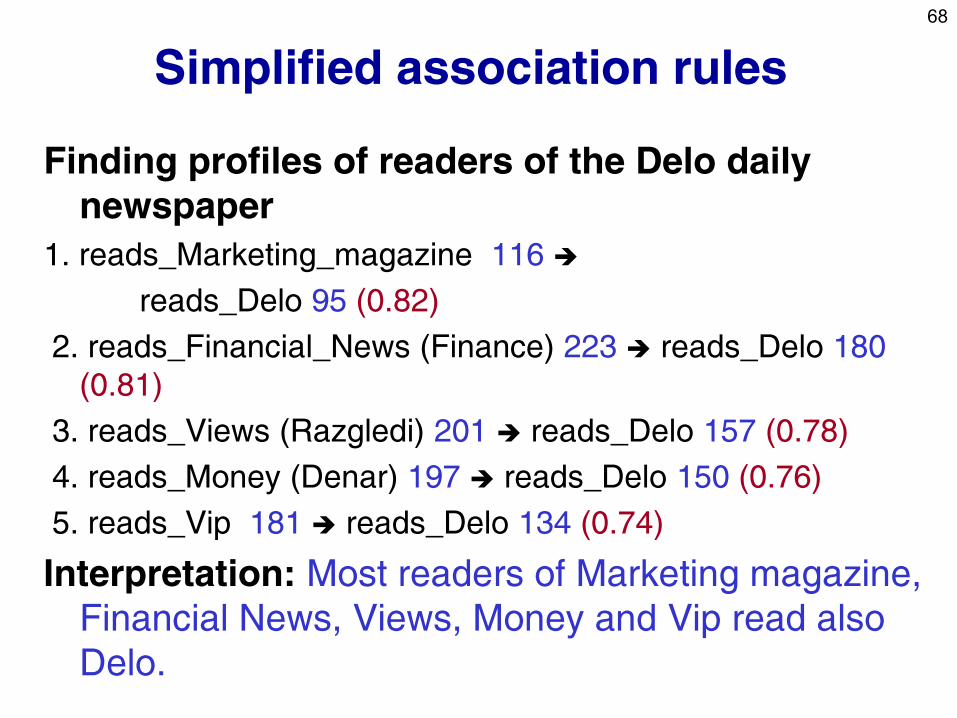
Simplified association rules
Finding profiles of readers of the Delo daily
newspaper
1. reads_Marketing_magazine 116
reads_Delo 95 (0.82)
2. reads_Financial_News (Finance) 223 reads_Delo 180
(0.81)
3. reads_Views (Razgledi) 201 reads_Delo 157 (0.78)
4. reads_Money (Denar) 197 reads_Delo 150 (0.76)
5. reads_Vip 181 reads_Delo 134 (0.74)
Interpretation: Most readers of Marketing magazine,
Financial News, Views, Money and Vip read also
Delo.
69
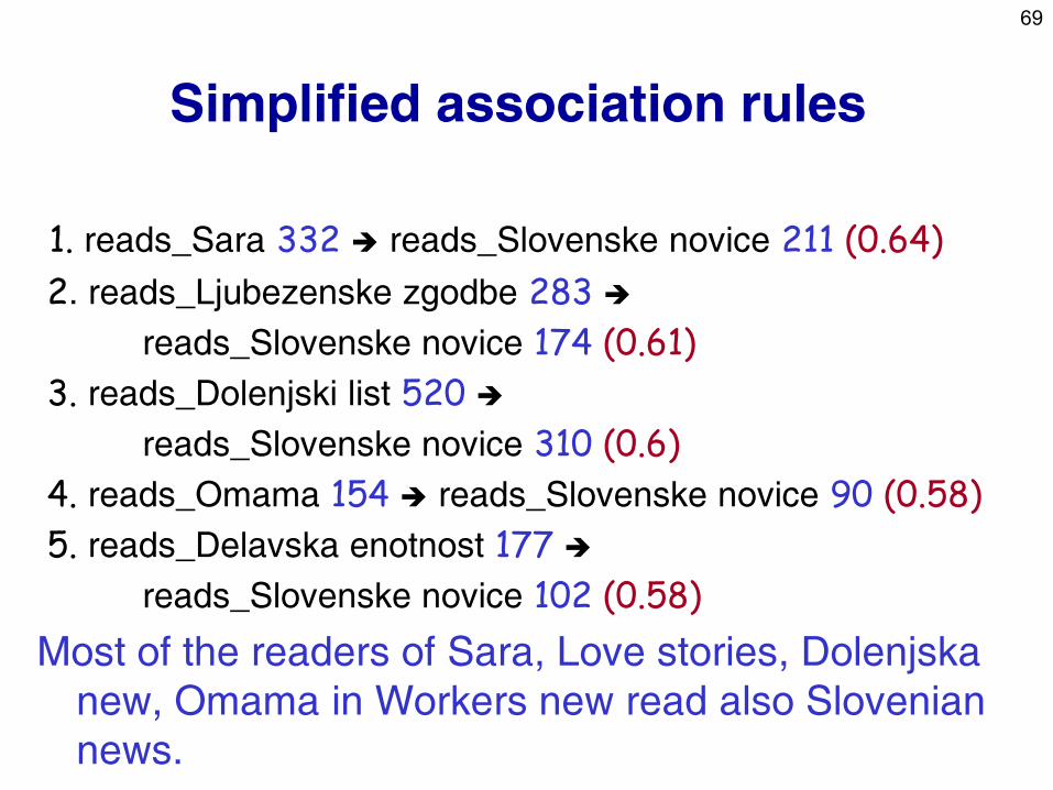
Simplified association rules
1. reads_Sara 332 reads_Slovenske novice 211 (0.64)
2. reads_Ljubezenske zgodbe 283
reads_Slovenske novice 174 (0.61)
3. reads_Dolenjski list 520
reads_Slovenske novice 310 (0.6)
4. reads_Omama 154 reads_Slovenske novice 90 (0.58)
5. reads_Delavska enotnost 177
reads_Slovenske novice 102 (0.58)
Most of the readers of Sara, Love stories, Dolenjska
new, Omama in Workers new read also Slovenian
news.
70
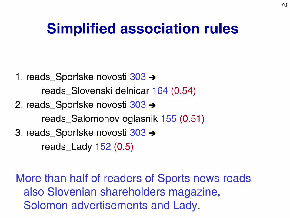
Simplified association rules
1. reads_Sportske novosti 303
reads_Slovenski delnicar 164 (0.54)
2. reads_Sportske novosti 303
reads_Salomonov oglasnik 155 (0.51)
3. reads_Sportske novosti 303
reads_Lady 152 (0.5)
More than half of readers of Sports news reads
also Slovenian shareholders magazine,
Solomon advertisements and Lady.
71
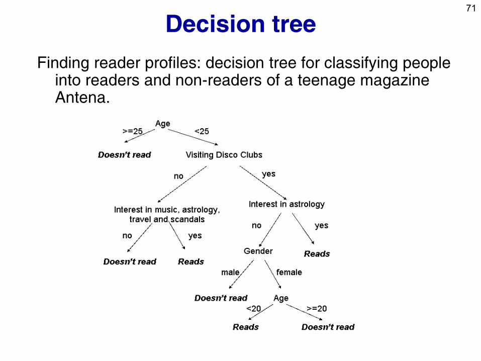
Decision tree
Finding reader profiles: decision tree for classifying people into readers and non-readers of a teenage magazine Antena.
72
Part I. Introduction
• Data Mining in a Nutshell
• Predictive and descriptive DM techniques
• Data Mining and the KDD process
• DM standards, tools and visualization
73
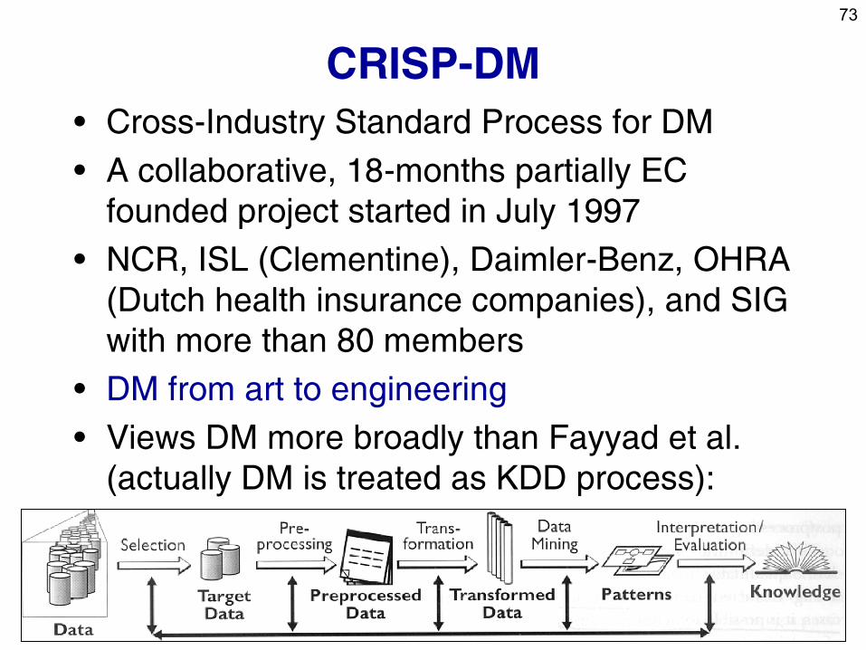
CRISP-DM
• Cross-Industry Standard Process for DM
• A collaborative, 18-months partially EC
founded project started in July 1997
• NCR, ISL (Clementine), Daimler-Benz, OHRA
(Dutch health insurance companies), and SIG
with more than 80 members
• DM from art to engineering
• Views DM more broadly than Fayyad et al.
(actually DM is treated as KDD process):
74
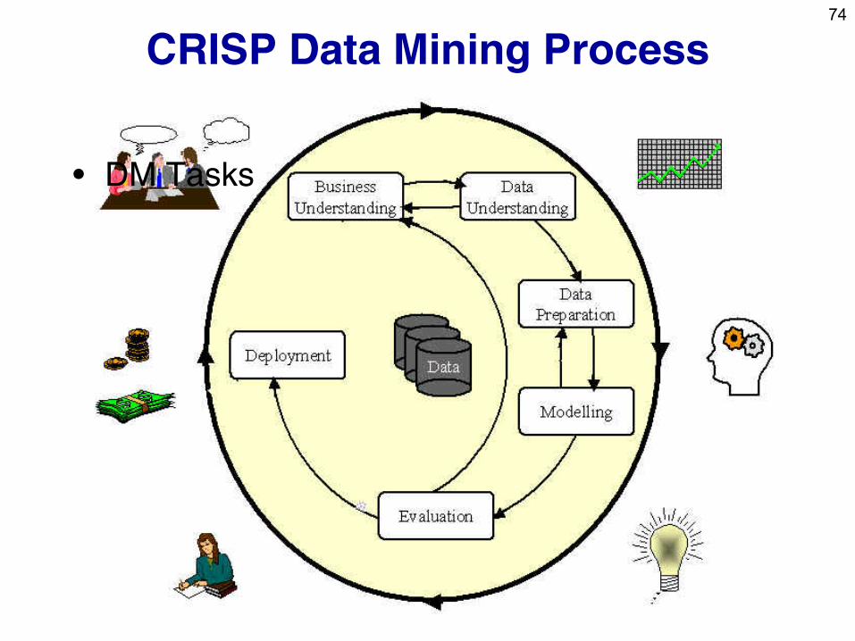
CRISP Data Mining Process
• DM Tasks
75
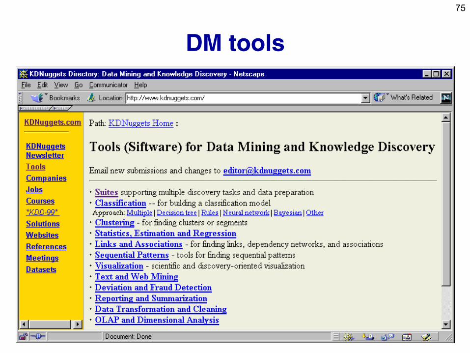
DM tools
76
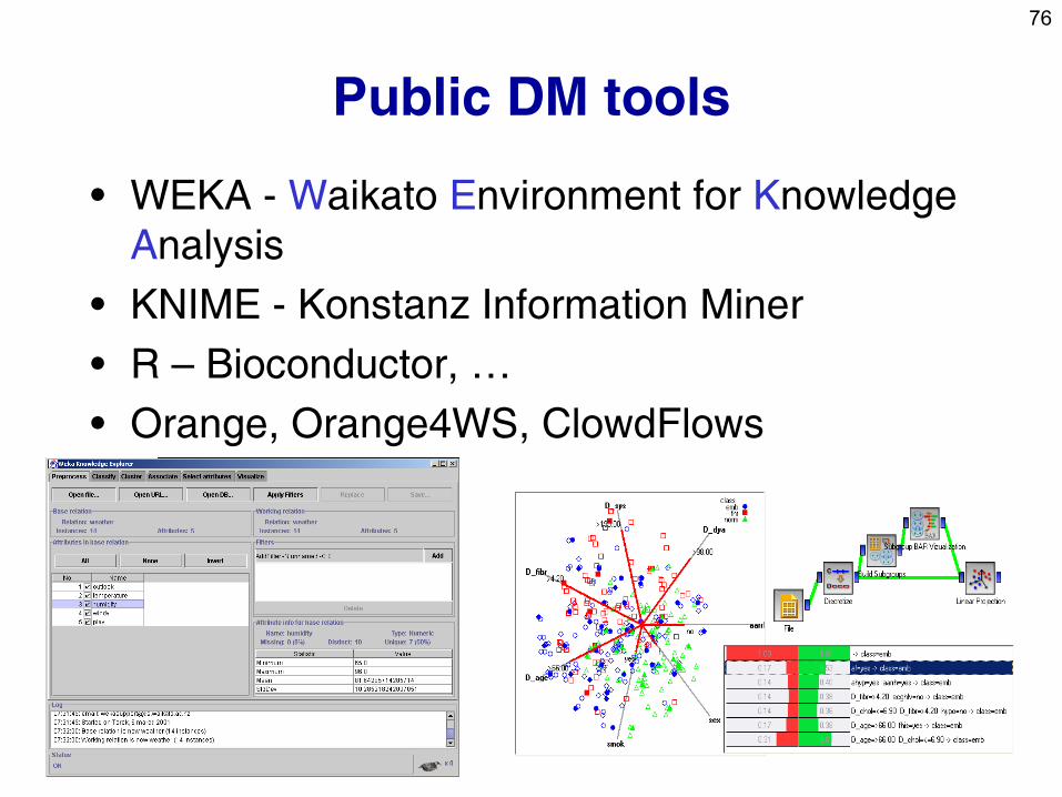
Public DM tools
• WEKA - Waikato Environment for Knowledge
Analysis
• KNIME - Konstanz Information Miner
• R – Bioconductor, …
• Orange, Orange4WS, ClowdFlows
77
Visualization
• can be used on its own (usually for
description and summarization tasks)
• can be used in combination with other DM
techniques, for example
– visualization of decision trees
– cluster visualization
– visualization of association rules
– subgroup visualization
78
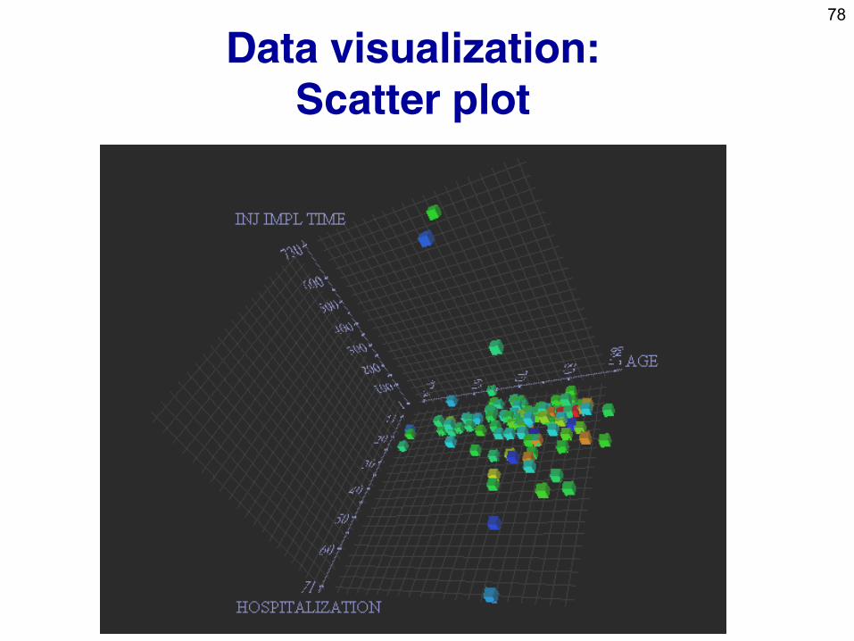
Data visualization:
Scatter plot
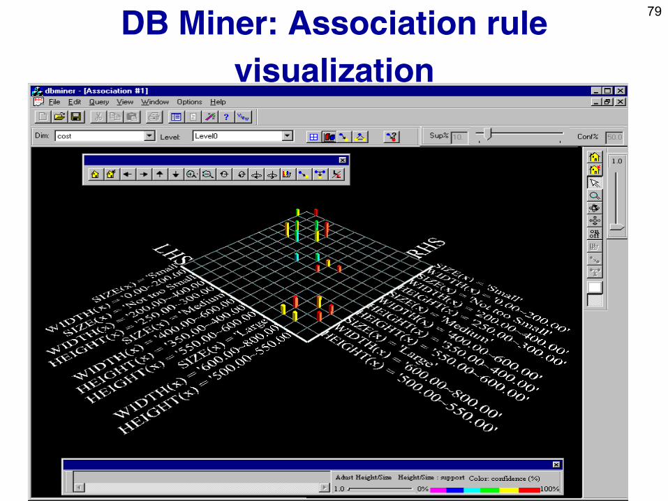
79
DB Miner: Association rule
visualization
80
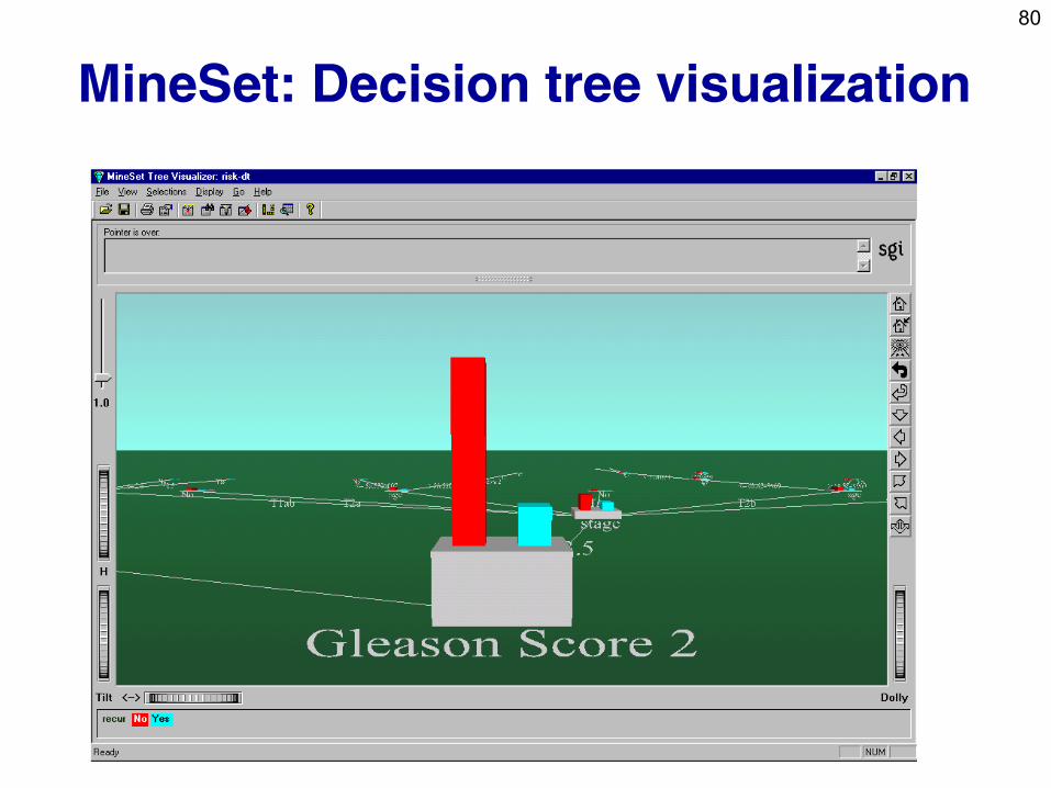
MineSet: Decision tree visualization
81
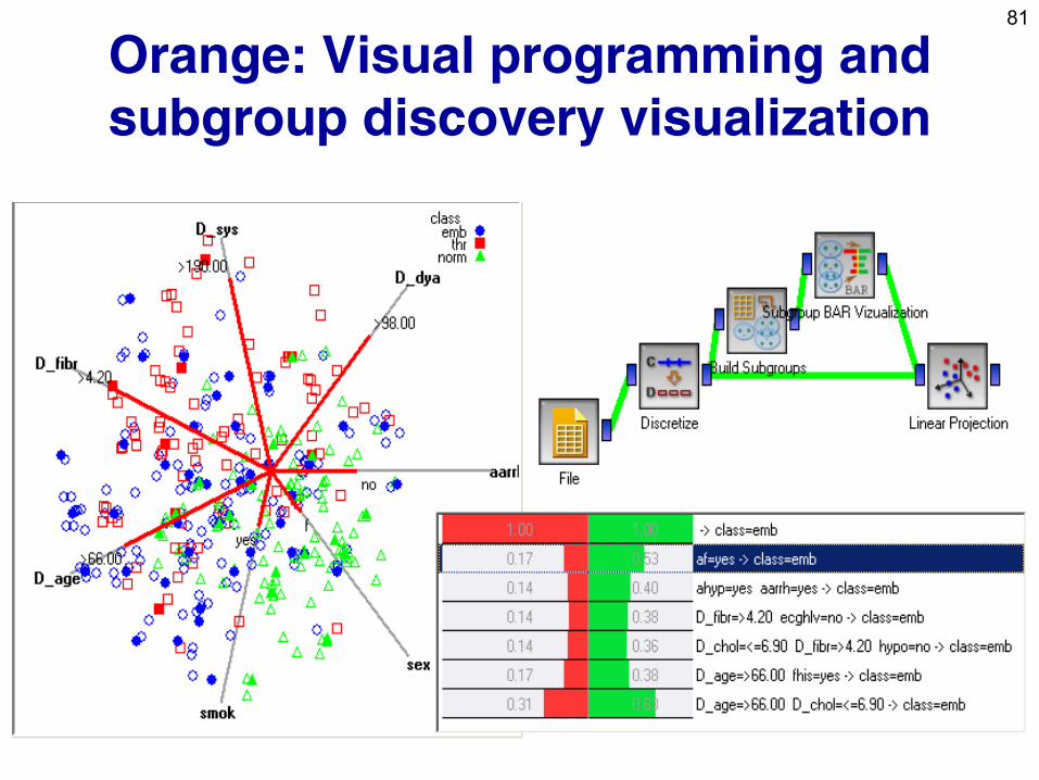
Orange: Visual programming and
subgroup discovery visualization
82
Part I: Summary
• KDD is the overall process of discovering useful
knowledge in data
– many steps including data preparation, cleaning,
transformation, pre-processing
• Data Mining is the data analysis phase in KDD
– DM takes only 15%-25% of the effort of the overall KDD
process
– employing techniques from machine learning and statistics
• Predictive and descriptive induction have different
goals: classifier vs. pattern discovery
• Many application areas, many powerful tools
available
83
Part II. Predictive DM techniques
• Naive Bayesian classifier
• Decision tree learning
• Classification rule learning
• Classifier evaluation
84
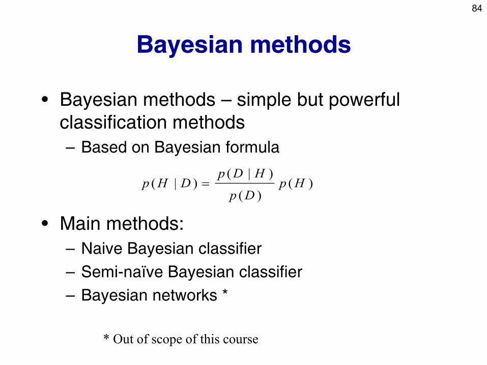
Bayesian methods
• Bayesian methods – simple but powerful
classification methods
– Based on Bayesian formula
• Main methods:
– Naive Bayesian classifier
– Semi-naïve Bayesian classifier
– Bayesian networks *
* Out of scope of this course
)()(
)|()|( Hp
Dp
HDpDHp
85
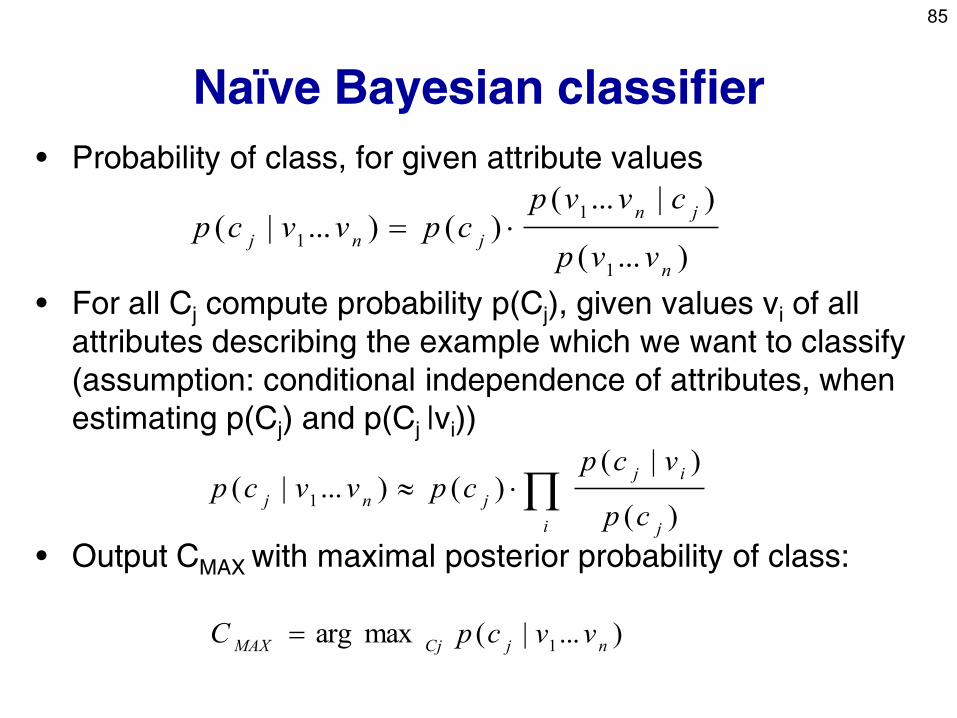
Naïve Bayesian classifier
• Probability of class, for given attribute values
• For all Cj compute probability p(Cj), given values vi of all
attributes describing the example which we want to classify
(assumption: conditional independence of attributes, when
estimating p(Cj) and p(Cj |vi))
• Output CMAX with maximal posterior probability of class:
)...(
)|...()()...|(
1
1
1
n
jn
jnjvvp
cvvpcpvvcp
i j
ij
jnjcp
vcpcpvvcp
)(
)|()()...|(
1
)...|(maxarg1 njCjMAXvvcpC
86
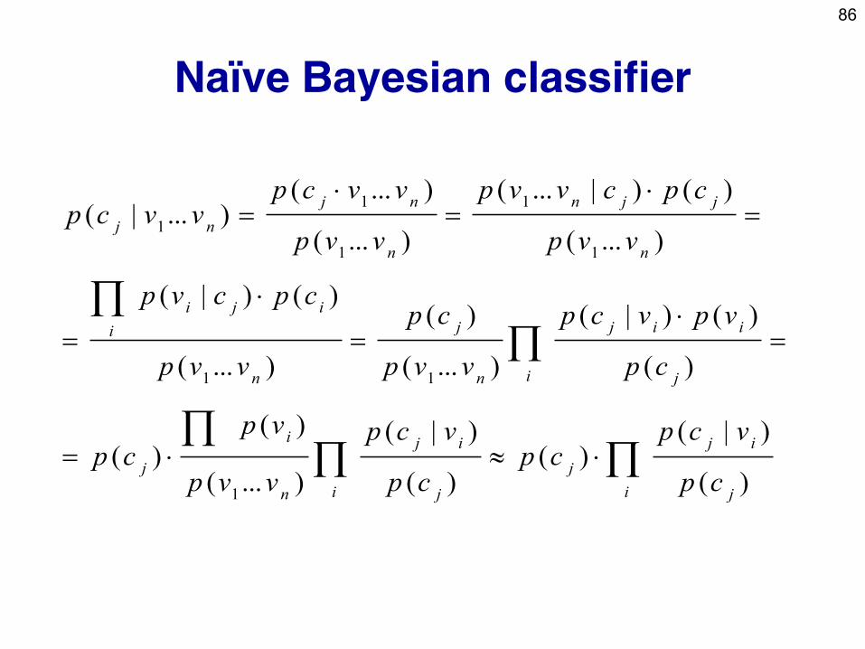
Naïve Bayesian classifier
i j
ij
j
i j
ij
n
i
j
i j
iij
n
j
n
i
iji
n
jjn
n
nj
nj
cp
vcpcp
cp
vcp
vvp
vpcp
cp
vpvcp
vvp
cp
vvp
cpcvp
vvp
cpcvvp
vvp
vvcpvvcp
)(
)|()(
)(
)|(
)...(
)()(
)(
)()|(
)...(
)(
)...(
)()|(
)...(
)()|...(
)...(
)...()...|(
1
11
1
1
1
1
1
87
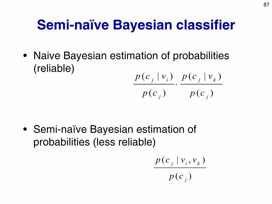
Semi-naïve Bayesian classifier
• Naive Bayesian estimation of probabilities
(reliable)
• Semi-naïve Bayesian estimation of
probabilities (less reliable)
)(
)|(
)(
)|(
j
kj
j
ij
cp
vcp
cp
vcp
)(
),|(
j
kij
cp
vvcp
88
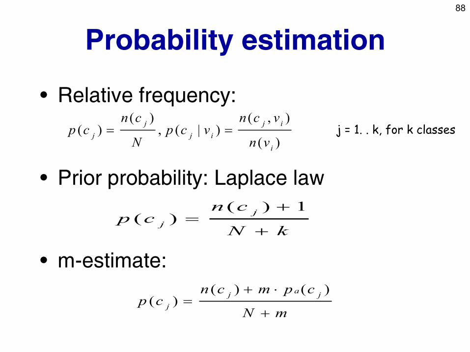
Probability estimation
• Relative frequency:
• Prior probability: Laplace law
• m-estimate:
)(
),()|(,
)()(
i
ij
ij
j
jvn
vcnvcp
N
cncp
mN
cpmcncp
ja
j
j
)()()(
kN
cncp
j
j
1)()(
j = 1. . k, for k classes
89
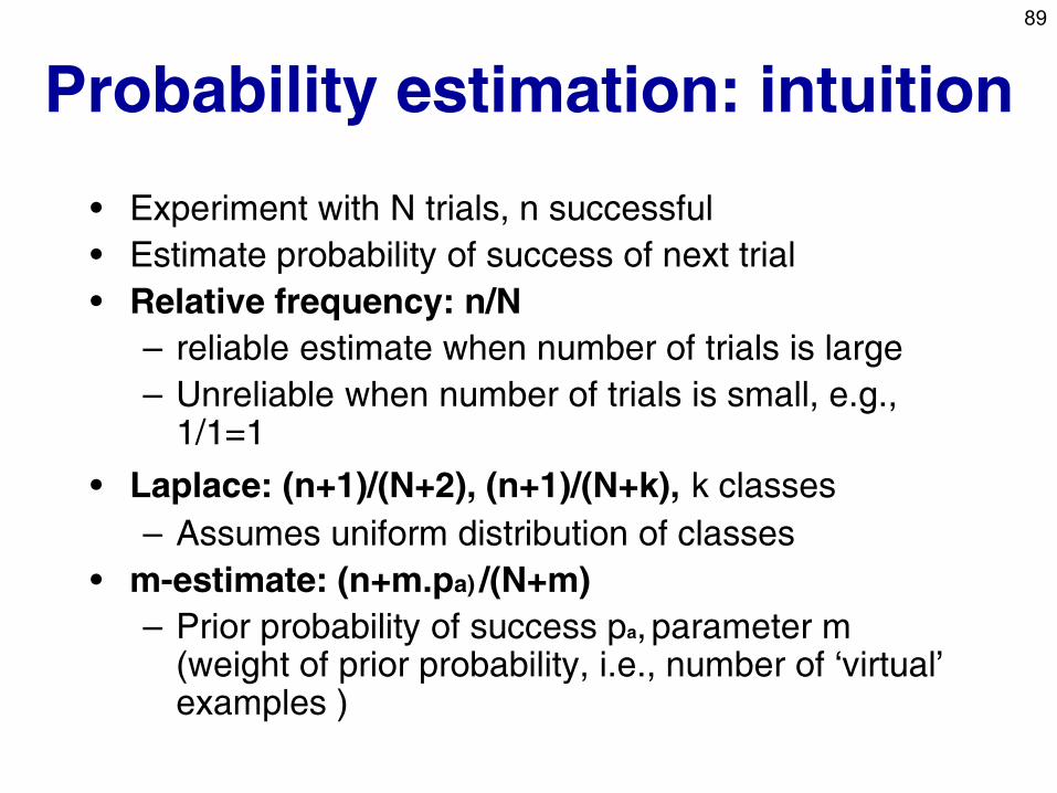
Probability estimation: intuition
• Experiment with N trials, n successful
• Estimate probability of success of next trial
• Relative frequency: n/N
– reliable estimate when number of trials is large
– Unreliable when number of trials is small, e.g., 1/1=1
• Laplace: (n+1)/(N+2), (n+1)/(N+k), k classes
– Assumes uniform distribution of classes
• m-estimate: (n+m.pa) /(N+m)
– Prior probability of success pa, parameter m (weight of prior probability, i.e., number of ‘virtual’ examples )
90
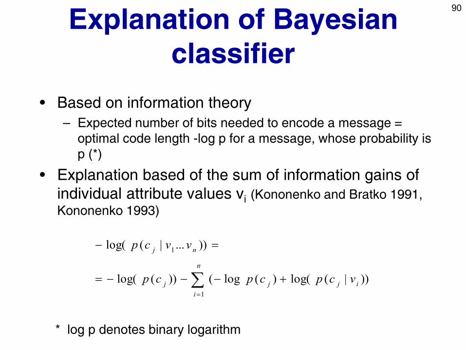
Explanation of Bayesian
classifier
• Based on information theory
– Expected number of bits needed to encode a message =
optimal code length -log p for a message, whose probability is
p (*)
• Explanation based of the sum of information gains of
individual attribute values vi (Kononenko and Bratko 1991,
Kononenko 1993)
* log p denotes binary logarithm
n
i
ijjj
nj
vcpcpcp
vvcp
1
1
))|(log()(log())(log(
))...|(log(
91
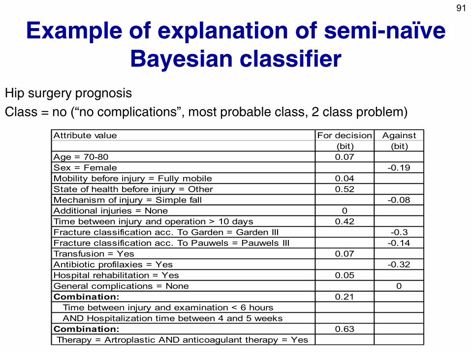
Example of explanation of semi-naïve
Bayesian classifier
Hip surgery prognosis
Class = no (“no complications”, most probable class, 2 class problem)
Attribute value For decision Against
(bit) (bit)
Age = 70-80 0.07
Sex = Female -0.19
Mobility before injury = Fully mobile 0.04
State of health before injury = Other 0.52
Mechanism of injury = Simple fall -0.08
Additional injuries = None 0
Time between injury and operation > 10 days 0.42
Fracture classification acc. To Garden = Garden III -0.3
Fracture classification acc. To Pauwels = Pauwels III -0.14
Transfusion = Yes 0.07
Antibiotic profilaxies = Yes -0.32
Hospital rehabilitation = Yes 0.05
General complications = None 0
Combination: 0.21
Time between injury and examination < 6 hours
AND Hospitalization time between 4 and 5 weeks
Combination: 0.63
Therapy = Artroplastic AND anticoagulant therapy = Yes
92
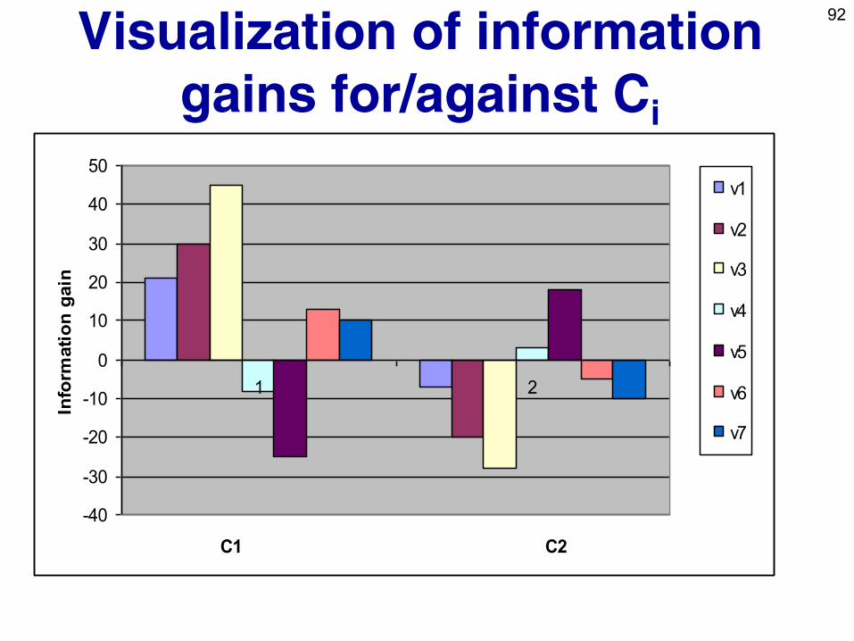
Visualization of information
gains for/against Ci
-40
-30
-20
-10
0
10
20
30
40
50
1 2
C1 C2
Info
rmati
on
gain
v1
v2
v3
v4
v5
v6
v7
93
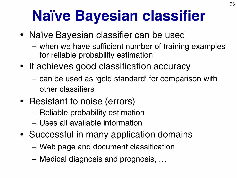
Naïve Bayesian classifier
• Naïve Bayesian classifier can be used – when we have sufficient number of training examples
for reliable probability estimation
• It achieves good classification accuracy
– can be used as ‘gold standard’ for comparison with
other classifiers
• Resistant to noise (errors) – Reliable probability estimation
– Uses all available information
• Successful in many application domains
– Web page and document classification
– Medical diagnosis and prognosis, …
94
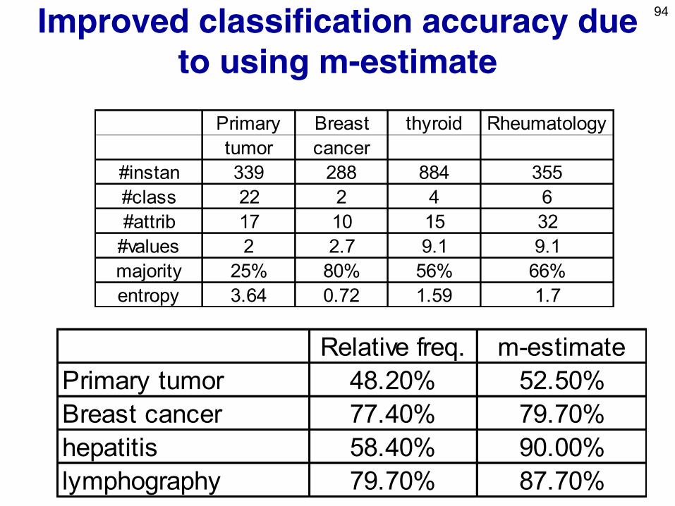
Improved classification accuracy due
to using m-estimate
Relative freq. m-estimate
Primary tumor 48.20% 52.50%
Breast cancer 77.40% 79.70%
hepatitis 58.40% 90.00%
lymphography 79.70% 87.70%
Primary Breast thyroid Rheumatology
tumor cancer
#instan 339 288 884 355
#class 22 2 4 6
#attrib 17 10 15 32
#values 2 2.7 9.1 9.1
majority 25% 80% 56% 66%
entropy 3.64 0.72 1.59 1.7
95
Part II. Predictive DM techniques
• Naïve Bayesian classifier
• Decision tree learning
• Classification rule learning
• Classifier evaluation

96
Illustrative example:
Contact lenses data
Person Age Spect. presc. Astigm. Tear prod. Lenses
O1 young myope no reduced NONE
O2 young myope no normal SOFT
O3 young myope yes reduced NONE
O4 young myope yes normal HARD
O5 young hypermetrope no reduced NONE
O6-O13 ... ... ... ... ...
O14 pre-presbyohypermetrope no normal SOFT
O15 pre-presbyohypermetrope yes reduced NONE
O16 pre-presbyohypermetrope yes normal NONE
O17 presbyopic myope no reduced NONE
O18 presbyopic myope no normal NONE
O19-O23 ... ... ... ... ...
O24 presbyopic hypermetrope yes normal NONE
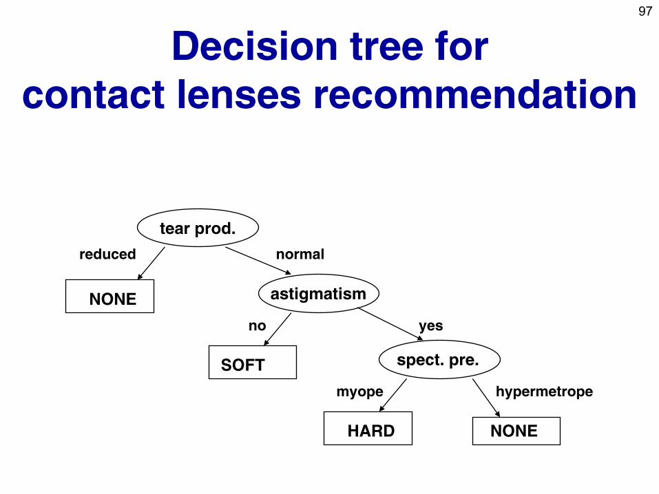
97
Decision tree for
contact lenses recommendation
tear prod.
astigmatism
spect. pre.
NONE
NONE
reduced
no yes
normal
hypermetrope
SOFT
myope
HARD
98
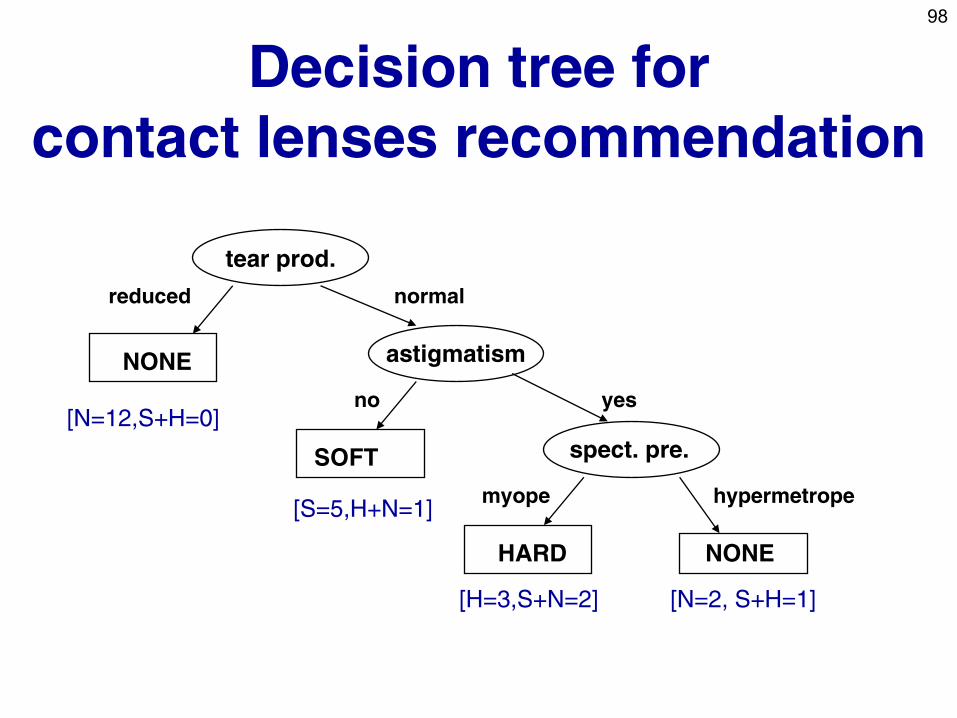
Decision tree for
contact lenses recommendation
tear prod.
astigmatism
spect. pre.
NONE
NONE
reduced
no yes
normal
hypermetrope
SOFT
myope
HARD
[N=12,S+H=0]
[N=2, S+H=1]
[S=5,H+N=1]
[H=3,S+N=2]
99
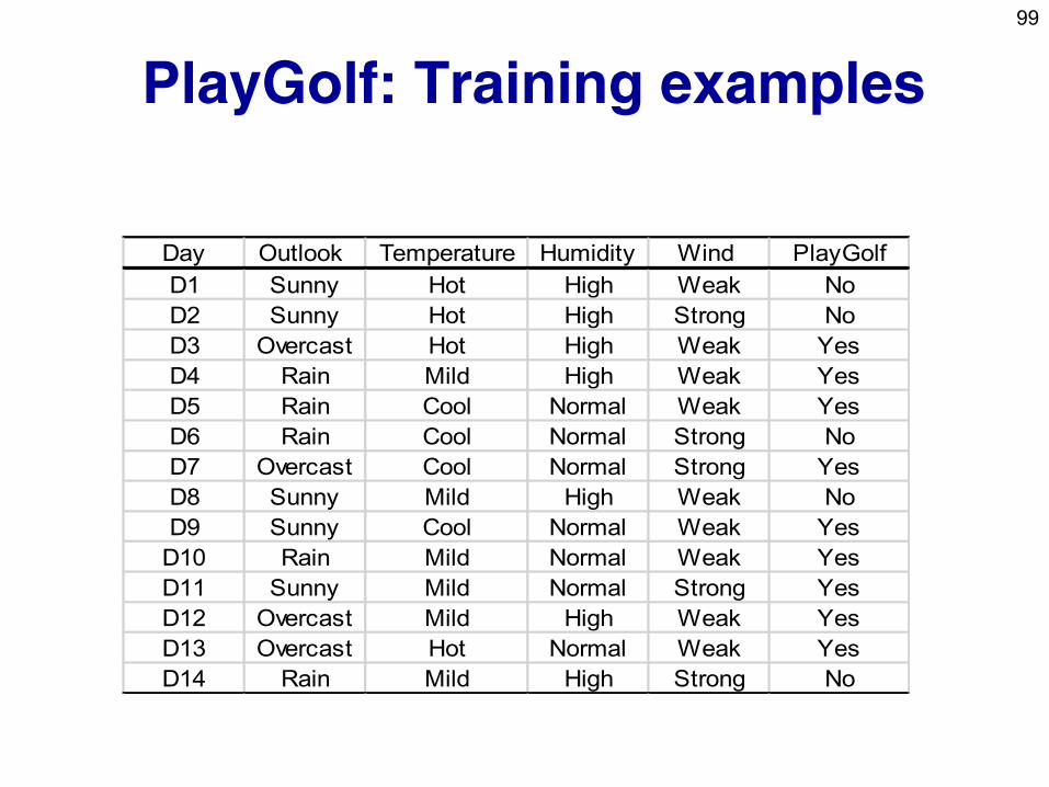
PlayGolf: Training examples
Day Outlook Temperature Humidity Wind PlayGolf
D1 Sunny Hot High Weak No
D2 Sunny Hot High Strong No
D3 Overcast Hot High Weak Yes
D4 Rain Mild High Weak Yes
D5 Rain Cool Normal Weak Yes
D6 Rain Cool Normal Strong No
D7 Overcast Cool Normal Strong Yes
D8 Sunny Mild High Weak No
D9 Sunny Cool Normal Weak Yes
D10 Rain Mild Normal Weak Yes
D11 Sunny Mild Normal Strong Yes
D12 Overcast Mild High Weak Yes
D13 Overcast Hot Normal Weak Yes
D14 Rain Mild High Strong No
100
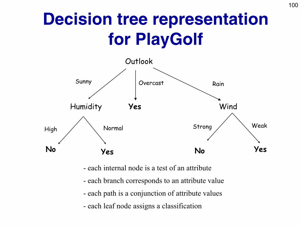
Decision tree representation
for PlayGolf Outlook
Humidity Wind Yes
Overcast Sunny Rain
High Normal Strong Weak
No Yes No Yes
- each internal node is a test of an attribute
- each branch corresponds to an attribute value
- each path is a conjunction of attribute values
- each leaf node assigns a classification
101
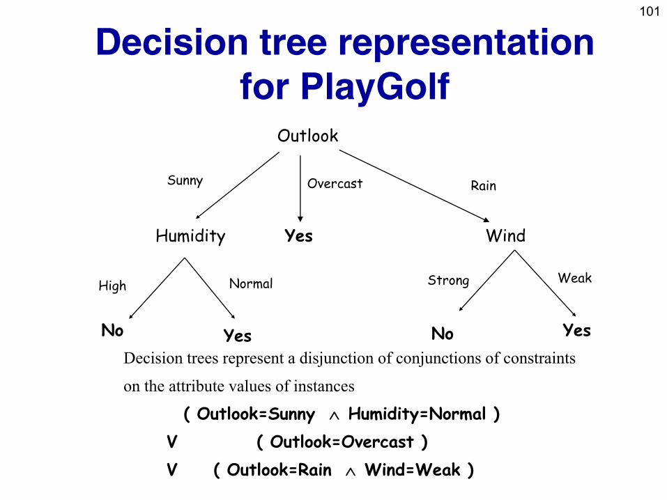
Decision tree representation
for PlayGolf Outlook
Humidity Wind Yes
Overcast Sunny Rain
High Normal Strong Weak
No Yes No Yes
Decision trees represent a disjunction of conjunctions of constraints
on the attribute values of instances
( Outlook=Sunny Humidity=Normal )
V ( Outlook=Overcast )
V ( Outlook=Rain Wind=Weak )
102
PlayGolf:
Other representations
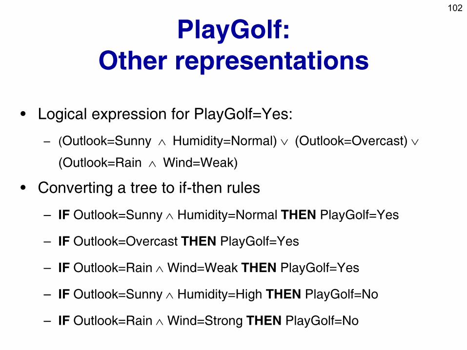
• Logical expression for PlayGolf=Yes:
– (Outlook=Sunny Humidity=Normal) (Outlook=Overcast)
(Outlook=Rain Wind=Weak)
• Converting a tree to if-then rules
– IF Outlook=Sunny Humidity=Normal THEN PlayGolf=Yes
– IF Outlook=Overcast THEN PlayGolf=Yes
– IF Outlook=Rain Wind=Weak THEN PlayGolf=Yes
– IF Outlook=Sunny Humidity=High THEN PlayGolf=No
– IF Outlook=Rain Wind=Strong THEN PlayGolf=No
103
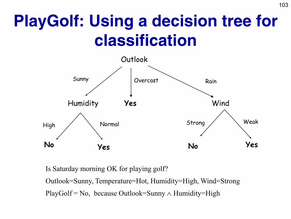
PlayGolf: Using a decision tree for
classification
Is Saturday morning OK for playing golf?
Outlook=Sunny, Temperature=Hot, Humidity=High, Wind=Strong
PlayGolf = No, because Outlook=Sunny Humidity=High
Outlook
Humidity Wind Yes
Overcast Sunny Rain
High Normal Strong Weak
No Yes No Yes
104
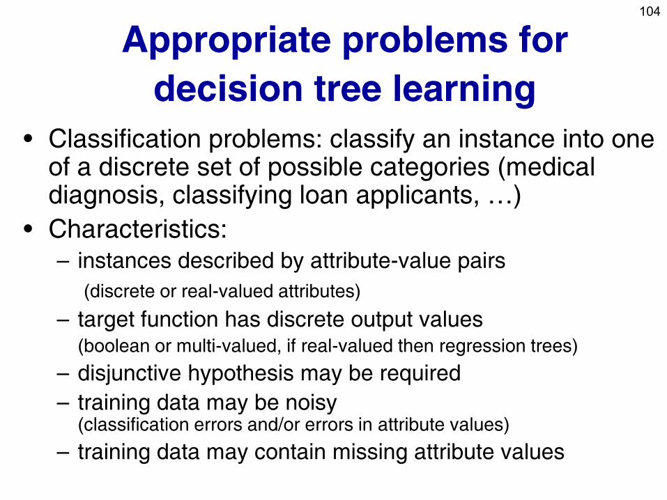
Appropriate problems for
decision tree learning
• Classification problems: classify an instance into one of a discrete set of possible categories (medical diagnosis, classifying loan applicants, …)
• Characteristics: – instances described by attribute-value pairs
(discrete or real-valued attributes)
– target function has discrete output values (boolean or multi-valued, if real-valued then regression trees)
– disjunctive hypothesis may be required
– training data may be noisy (classification errors and/or errors in attribute values)
– training data may contain missing attribute values
105
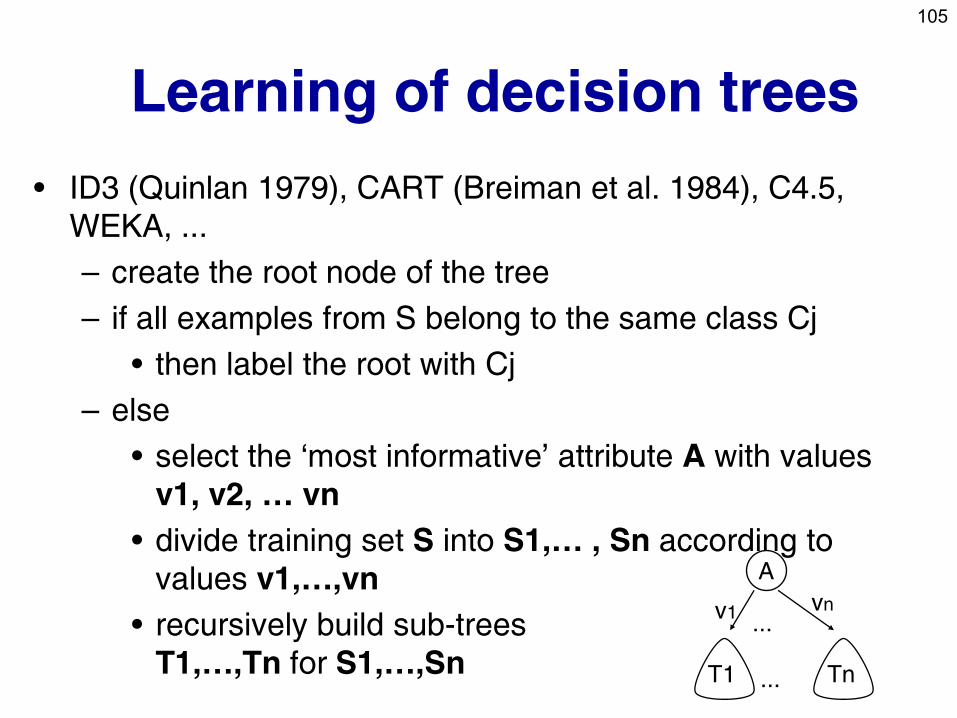
Learning of decision trees
• ID3 (Quinlan 1979), CART (Breiman et al. 1984), C4.5,
WEKA, ...
– create the root node of the tree
– if all examples from S belong to the same class Cj
• then label the root with Cj
– else
• select the ‘most informative’ attribute A with values
v1, v2, … vn
• divide training set S into S1,… , Sn according to
values v1,…,vn
• recursively build sub-trees
T1,…,Tn for S1,…,Sn
A
...
... T1 Tn
vn v1
106
Search heuristics in ID3
• Central choice in ID3: Which attribute to test at each node in the tree ? The attribute that is most useful for classifying examples.
• Define a statistical property, called information gain, measuring how well a given attribute separates the training examples w.r.t their target classification.
• First define a measure commonly used in information theory, called entropy, to characterize the (im)purity of an arbitrary collection of examples.
107
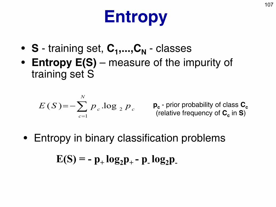
Entropy
• S - training set, C1,...,CN - classes
• Entropy E(S) – measure of the impurity of training set S
N
c
ccppSE
1
2log.)( pc - prior probability of class Cc
(relative frequency of Cc in S)
E(S) = - p+ log2p+ - p- log2p-
• Entropy in binary classification problems
108
Entropy
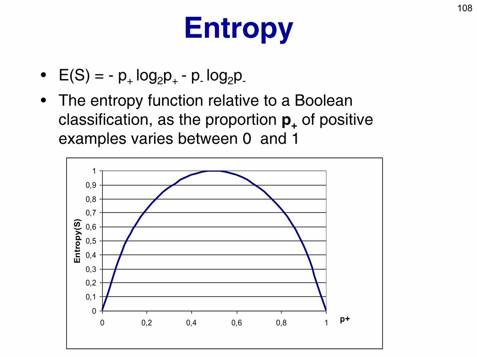
• E(S) = - p+ log2p+ - p- log2p-
• The entropy function relative to a Boolean
classification, as the proportion p+ of positive
examples varies between 0 and 1
0
0,1
0,2
0,3
0,4
0,5
0,6
0,7
0,8
0,9
1
0 0,2 0,4 0,6 0,8 1 p+
En
tro
py
(S)
109
Entropy – why ?
• Entropy E(S) = expected amount of information (in
bits) needed to assign a class to a randomly drawn
object in S (under the optimal, shortest-length
code)
• Why ?
• Information theory: optimal length code assigns
- log2p bits to a message having probability p
• So, in binary classification problems, the expected
number of bits to encode + or – of a random
member of S is:
p+ ( - log2p+ ) + p- ( - log2p- ) = - p+ log2p+ - p- log2p-
110
PlayGolf: Entropy
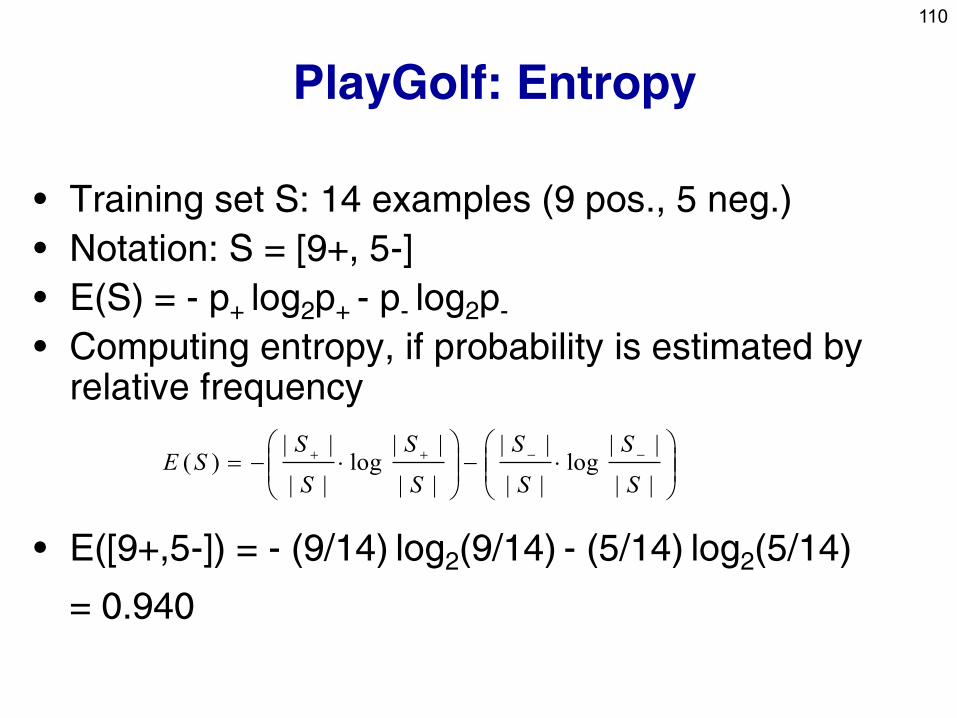
• Training set S: 14 examples (9 pos., 5 neg.)
• Notation: S = [9+, 5-]
• E(S) = - p+ log2p+ - p- log2p-
• Computing entropy, if probability is estimated by relative frequency
• E([9+,5-]) = - (9/14) log2(9/14) - (5/14) log2(5/14)
= 0.940
||
||log
||
||
||
||log
||
||)(
S
S
S
S
S
S
S
SSE
111
PlayGolf: Entropy
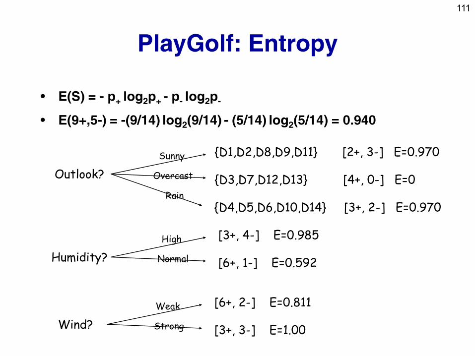
• E(S) = - p+ log2p+ - p- log2p-
• E(9+,5-) = -(9/14) log2(9/14) - (5/14) log2(5/14) = 0.940
Outlook?
{D1,D2,D8,D9,D11} [2+, 3-] E=0.970
{D3,D7,D12,D13} [4+, 0-] E=0
{D4,D5,D6,D10,D14} [3+, 2-] E=0.970
Sunny
Overcast
Rain
Humidity?
[3+, 4-] E=0.985
[6+, 1-] E=0.592
High
Normal
Wind?
[6+, 2-] E=0.811
[3+, 3-] E=1.00
Weak
Strong
112
Information gain
search heuristic
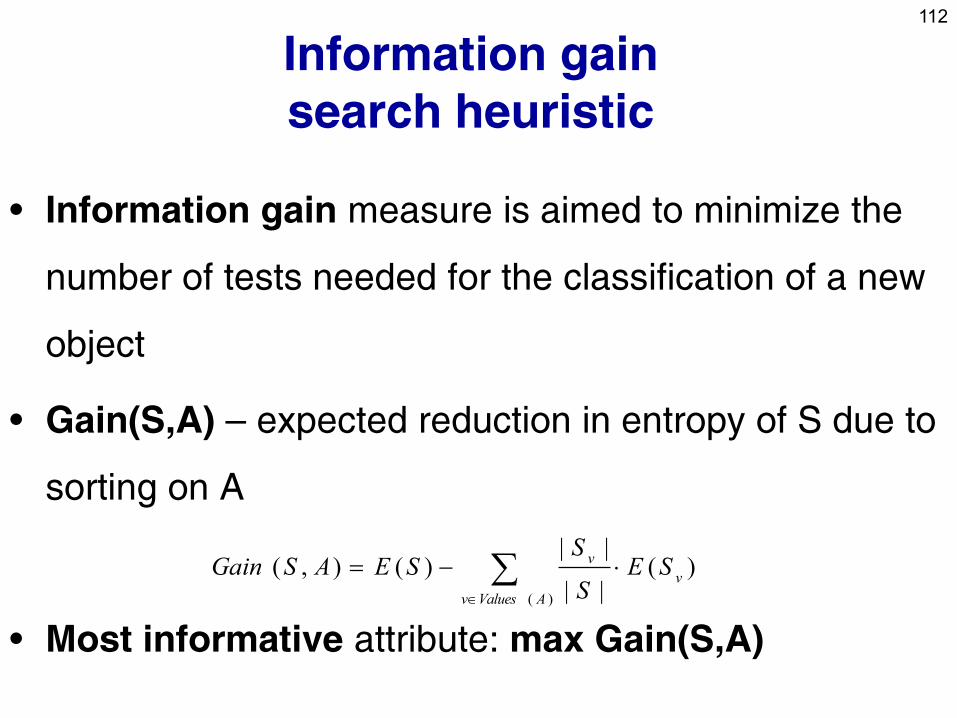
• Information gain measure is aimed to minimize the
number of tests needed for the classification of a new
object
• Gain(S,A) – expected reduction in entropy of S due to
sorting on A
• Most informative attribute: max Gain(S,A)
)(||
||)(),(
)(
v
AValuesv
vSE
S
SSEASGain
113
Information gain
search heuristic
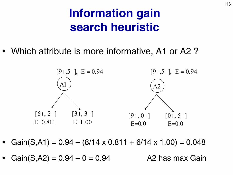
• Which attribute is more informative, A1 or A2 ?
• Gain(S,A1) = 0.94 – (8/14 x 0.811 + 6/14 x 1.00) = 0.048
• Gain(S,A2) = 0.94 – 0 = 0.94 A2 has max Gain
A1
[9,5], E 0.94
[3, 3] [6, 2]
E0.811 E1.00
A2
[0, 5] [9, 0]
E0.0 E0.0
[9,5], E 0.94
114
PlayGolf: Information gain
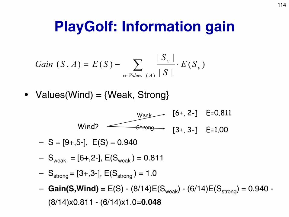
• Values(Wind) = {Weak, Strong}
– S = [9+,5-], E(S) = 0.940
– Sweak = [6+,2-], E(Sweak ) = 0.811
– Sstrong = [3+,3-], E(Sstrong ) = 1.0
– Gain(S,Wind) = E(S) - (8/14)E(Sweak) - (6/14)E(Sstrong) = 0.940 -
(8/14)x0.811 - (6/14)x1.0=0.048
)(||
||)(),(
)(
v
AValuesv
vSE
S
SSEASGain
Wind?
[6+, 2-] E=0.811
[3+, 3-] E=1.00
Weak
Strong
115
PlayGolf: Information gain
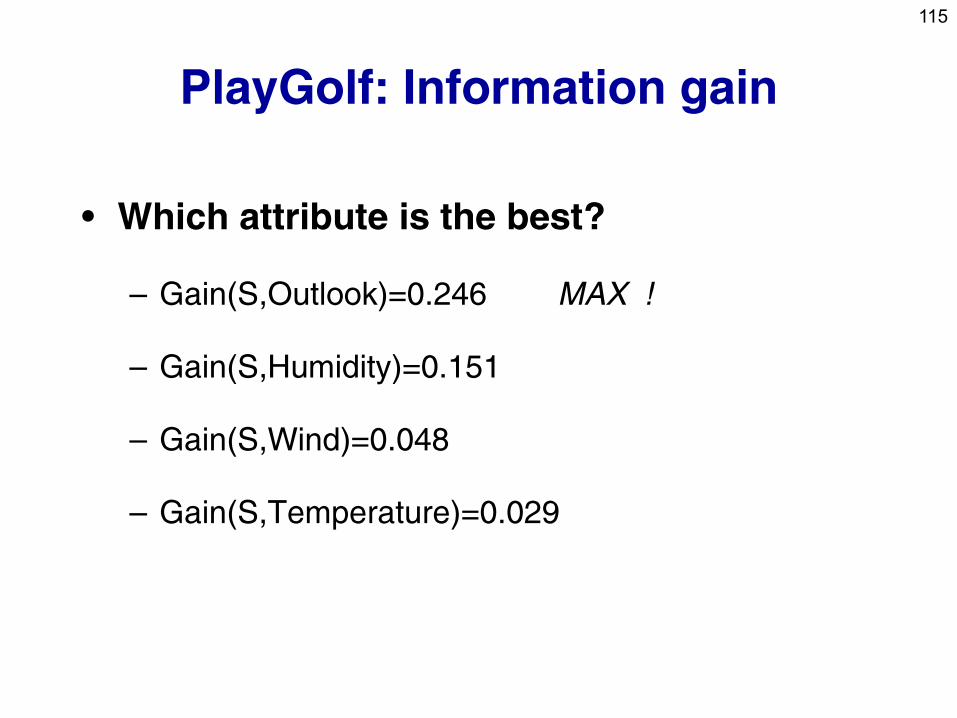
• Which attribute is the best?
– Gain(S,Outlook)=0.246 MAX !
– Gain(S,Humidity)=0.151
– Gain(S,Wind)=0.048
– Gain(S,Temperature)=0.029
116
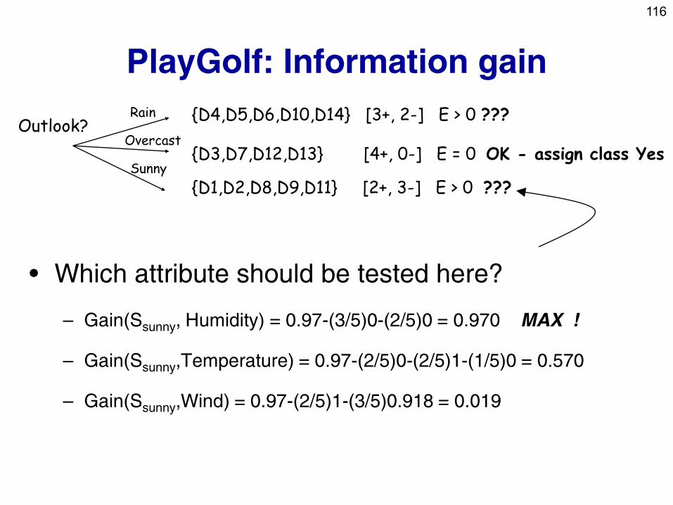
PlayGolf: Information gain
• Which attribute should be tested here?
– Gain(Ssunny, Humidity) = 0.97-(3/5)0-(2/5)0 = 0.970 MAX !
– Gain(Ssunny,Temperature) = 0.97-(2/5)0-(2/5)1-(1/5)0 = 0.570
– Gain(Ssunny,Wind) = 0.97-(2/5)1-(3/5)0.918 = 0.019
Outlook?
{D1,D2,D8,D9,D11} [2+, 3-] E > 0 ???
{D3,D7,D12,D13} [4+, 0-] E = 0 OK - assign class Yes Sunny
Overcast
{D4,D5,D6,D10,D14} [3+, 2-] E > 0 ??? Rain
117
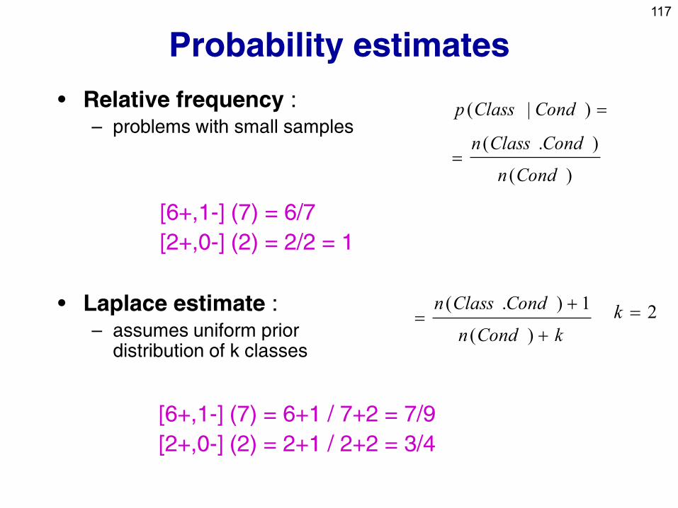
Probability estimates
• Relative frequency : – problems with small samples
• Laplace estimate : – assumes uniform prior
distribution of k classes
)(
).(
)|(
Condn
CondClassn
CondClassp
kCondn
CondClassn
)(
1).(2k
[6+,1-] (7) = 6/7
[2+,0-] (2) = 2/2 = 1
[6+,1-] (7) = 6+1 / 7+2 = 7/9
[2+,0-] (2) = 2+1 / 2+2 = 3/4
118
Heuristic search in ID3
• Search bias: Search the space of decision trees from simplest to increasingly complex (greedy search, no backtracking, prefer small trees)
• Search heuristics: At a node, select the attribute that is most useful for classifying examples, split the node accordingly
• Stopping criteria: A node becomes a leaf
– if all examples belong to same class Cj, label the leaf with Cj
– if all attributes were used, label the leaf with the most common value Ck of examples in the node
• Extension to ID3: handling noise - tree pruning
119
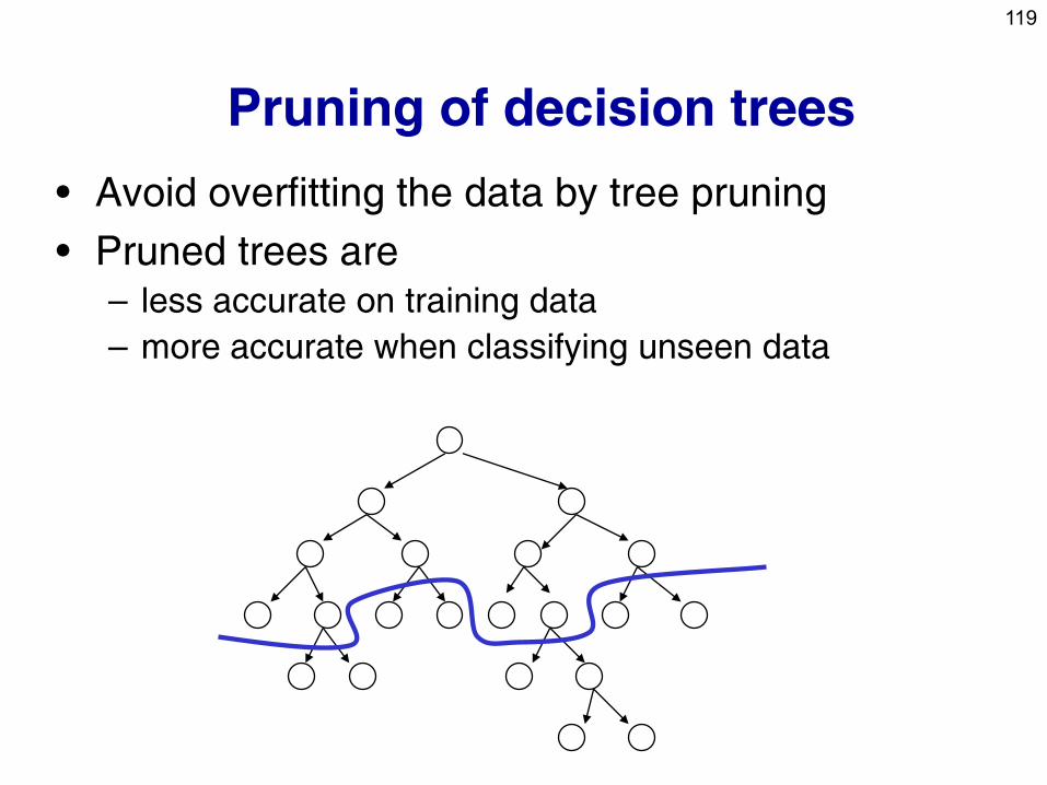
Pruning of decision trees
• Avoid overfitting the data by tree pruning
• Pruned trees are – less accurate on training data
– more accurate when classifying unseen data
120
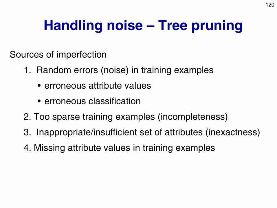
Handling noise – Tree pruning
Sources of imperfection
1. Random errors (noise) in training examples
• erroneous attribute values
• erroneous classification
2. Too sparse training examples (incompleteness)
3. Inappropriate/insufficient set of attributes (inexactness)
4. Missing attribute values in training examples
121
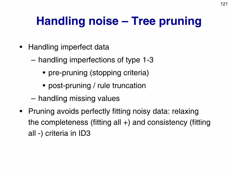
Handling noise – Tree pruning
• Handling imperfect data
– handling imperfections of type 1-3
• pre-pruning (stopping criteria)
• post-pruning / rule truncation
– handling missing values
• Pruning avoids perfectly fitting noisy data: relaxing
the completeness (fitting all +) and consistency (fitting
all -) criteria in ID3
122
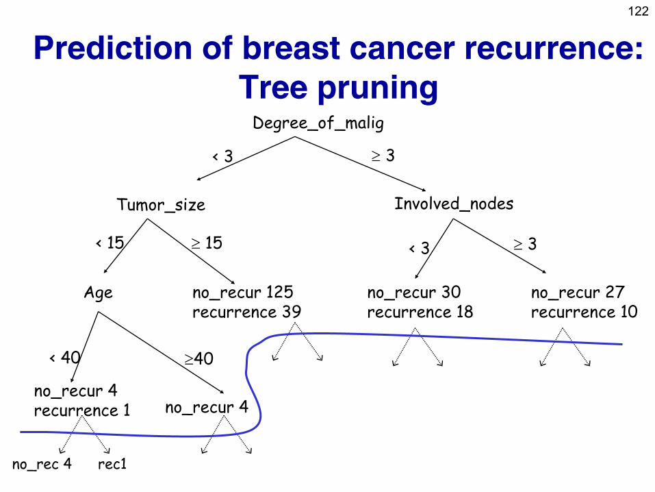
Prediction of breast cancer recurrence:
Tree pruning Degree_of_malig
Tumor_size
Age no_recur 125 recurrence 39
no_recur 4 recurrence 1 no_recur 4
Involved_nodes
no_recur 30 recurrence 18
no_recur 27 recurrence 10
< 3 3
< 15 15 < 3 3
< 40 40
no_rec 4 rec1
123
Accuracy and error
• Accuracy: percentage of correct classifications
– on the training set
– on unseen instances
• How accurate is a decision tree when classifying unseen
instances
– An estimate of accuracy on unseen instances can be computed,
e.g., by averaging over 4 runs:
• split the example set into training set (e.g. 70%) and test set (e.g. 30%)
• induce a decision tree from training set, compute its accuracy on test
set
• Error = 1 - Accuracy
• High error may indicate data overfitting
124
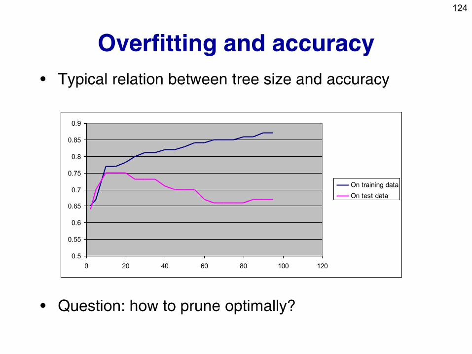
Overfitting and accuracy
• Typical relation between tree size and accuracy
• Question: how to prune optimally?
0.5
0.55
0.6
0.65
0.7
0.75
0.8
0.85
0.9
0 20 40 60 80 100 120
On training data
On test data
125
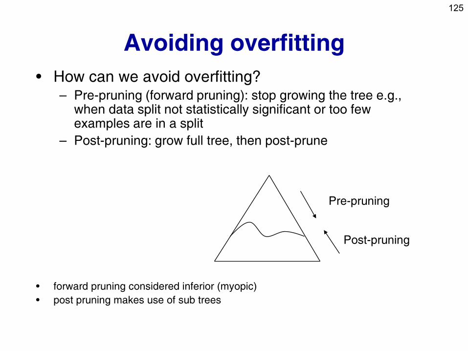
Avoiding overfitting
• How can we avoid overfitting? – Pre-pruning (forward pruning): stop growing the tree e.g.,
when data split not statistically significant or too few examples are in a split
– Post-pruning: grow full tree, then post-prune
• forward pruning considered inferior (myopic)
• post pruning makes use of sub trees
Pre-pruning
Post-pruning
126
How to select the “best” tree
• Measure performance over training data (e.g., pessimistic post-pruning, Quinlan 1993)
• Measure performance over separate validation data set (e.g., reduced error pruning, Quinlan 1987) – until further pruning is harmful DO:
• for each node evaluate the impact of replacing a subtree by a leaf, assigning the majority class of examples in the leaf, if the pruned tree performs no worse than the original over the validation set
• greedily select the node whose removal most improves tree accuracy over the validation set
• MDL: minimize size(tree)+size(misclassifications(tree))
127
Selected decision/regression
tree learners
• Decision tree learners
– ID3 (Quinlan 1979)
– CART (Breiman et al. 1984)
– Assistant (Cestnik et al. 1987)
– C4.5 (Quinlan 1993), C5 (See5, Quinlan)
– J48 (available in WEKA)
• Regression tree learners, model tree learners
– M5, M5P (implemented in WEKA)
128
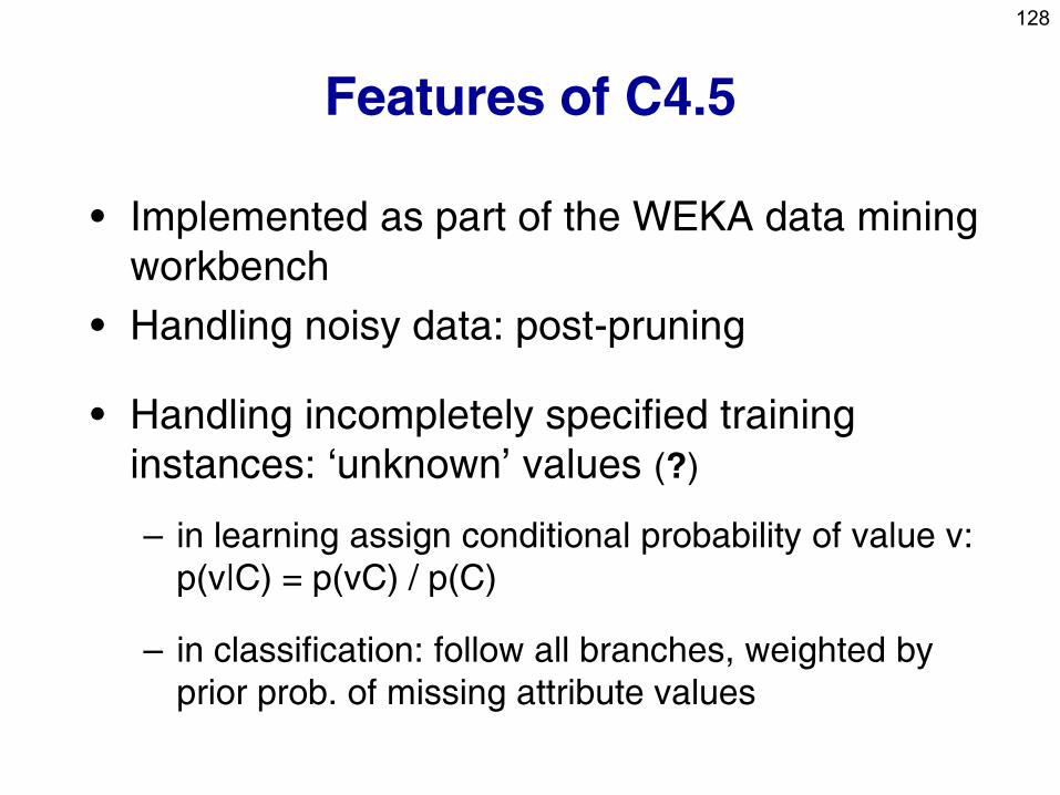
Features of C4.5
• Implemented as part of the WEKA data mining
workbench
• Handling noisy data: post-pruning
• Handling incompletely specified training
instances: ‘unknown’ values (?)
– in learning assign conditional probability of value v:
p(v|C) = p(vC) / p(C)
– in classification: follow all branches, weighted by
prior prob. of missing attribute values
129
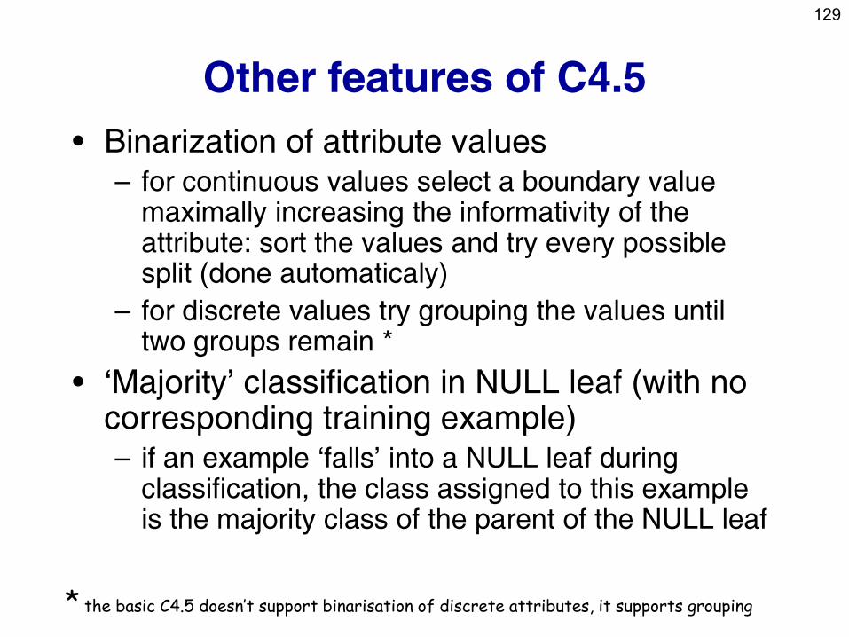
Other features of C4.5
• Binarization of attribute values – for continuous values select a boundary value
maximally increasing the informativity of the attribute: sort the values and try every possible split (done automaticaly)
– for discrete values try grouping the values until two groups remain *
• ‘Majority’ classification in NULL leaf (with no corresponding training example) – if an example ‘falls’ into a NULL leaf during
classification, the class assigned to this example is the majority class of the parent of the NULL leaf
* the basic C4.5 doesn’t support binarisation of discrete attributes, it supports grouping
130
Part II. Predictive DM techniques
• Naïve Bayesian classifier
• Decision tree learning
• Classification rule learning
• Classifier evaluation
131
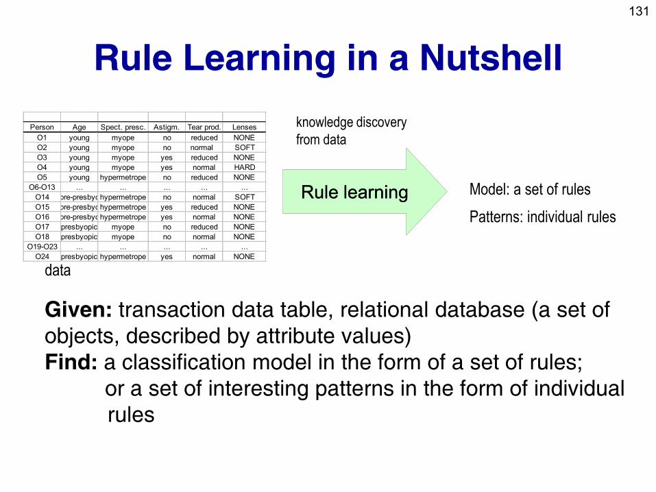
Rule Learning in a Nutshell
data
Rule learningRule learning
knowledge discovery
from data
Model: a set of rules
Patterns: individual rules
Given: transaction data table, relational database (a set of
objects, described by attribute values)
Find: a classification model in the form of a set of rules;
or a set of interesting patterns in the form of individual
rules
Person Age Spect. presc. Astigm. Tear prod. Lenses
O1 young myope no reduced NONE
O2 young myope no normal SOFT
O3 young myope yes reduced NONE
O4 young myope yes normal HARD
O5 young hypermetrope no reduced NONE
O6-O13 ... ... ... ... ...
O14 pre-presbyohypermetrope no normal SOFT
O15 pre-presbyohypermetrope yes reduced NONE
O16 pre-presbyohypermetrope yes normal NONE
O17 presbyopic myope no reduced NONE
O18 presbyopic myope no normal NONE
O19-O23 ... ... ... ... ...
O24 presbyopic hypermetrope yes normal NONE
132
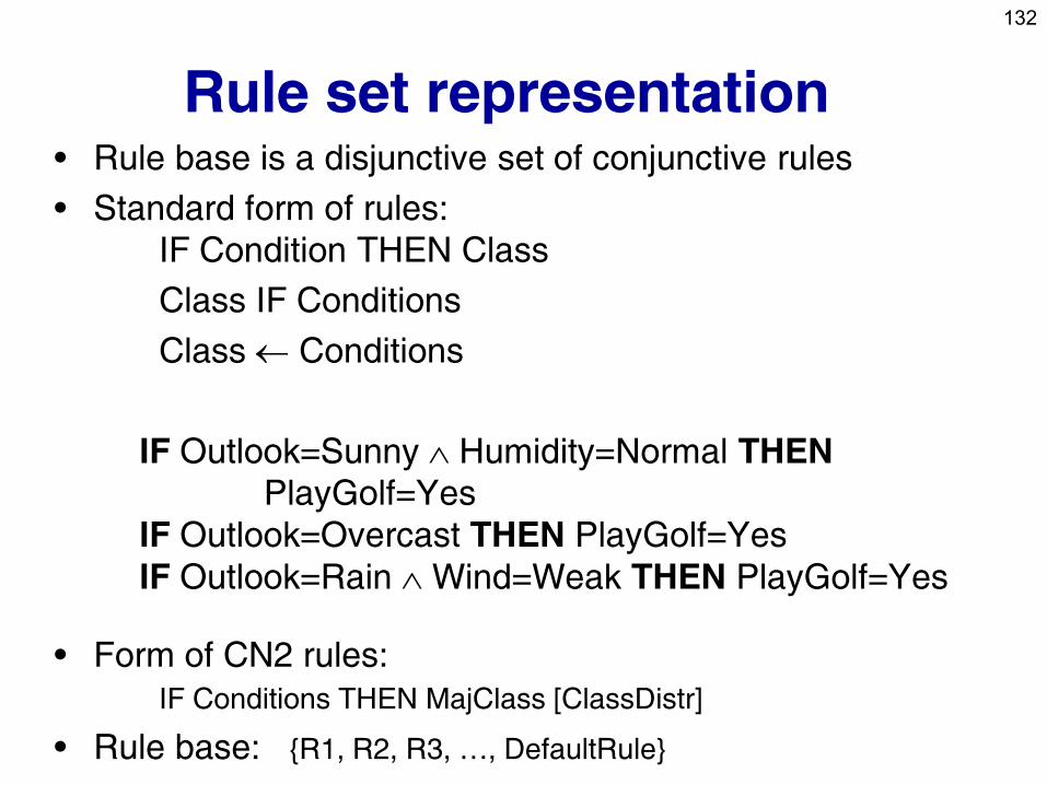
Rule set representation • Rule base is a disjunctive set of conjunctive rules
• Standard form of rules:
IF Condition THEN Class
Class IF Conditions
Class Conditions
IF Outlook=Sunny Humidity=Normal THEN
PlayGolf=Yes
IF Outlook=Overcast THEN PlayGolf=Yes
IF Outlook=Rain Wind=Weak THEN PlayGolf=Yes
• Form of CN2 rules:
IF Conditions THEN MajClass [ClassDistr]
• Rule base: {R1, R2, R3, …, DefaultRule}
133
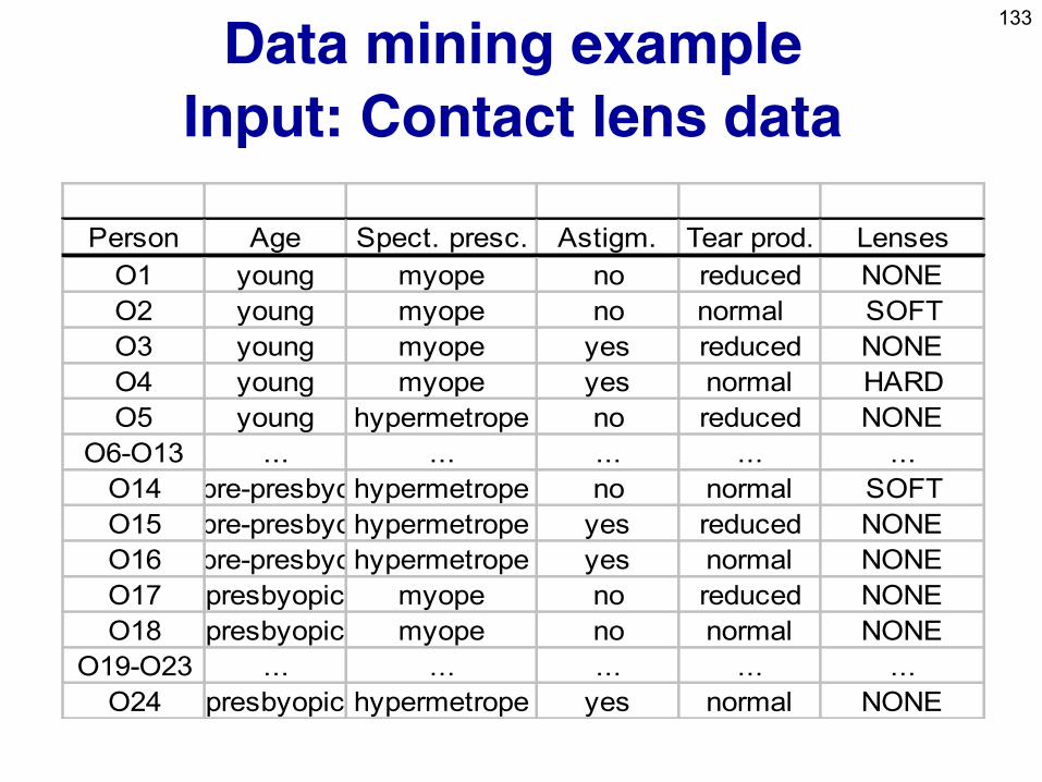
Data mining example
Input: Contact lens data
Person Age Spect. presc. Astigm. Tear prod. Lenses
O1 young myope no reduced NONE
O2 young myope no normal SOFT
O3 young myope yes reduced NONE
O4 young myope yes normal HARD
O5 young hypermetrope no reduced NONE
O6-O13 ... ... ... ... ...
O14 pre-presbyohypermetrope no normal SOFT
O15 pre-presbyohypermetrope yes reduced NONE
O16 pre-presbyohypermetrope yes normal NONE
O17 presbyopic myope no reduced NONE
O18 presbyopic myope no normal NONE
O19-O23 ... ... ... ... ...
O24 presbyopic hypermetrope yes normal NONE
134
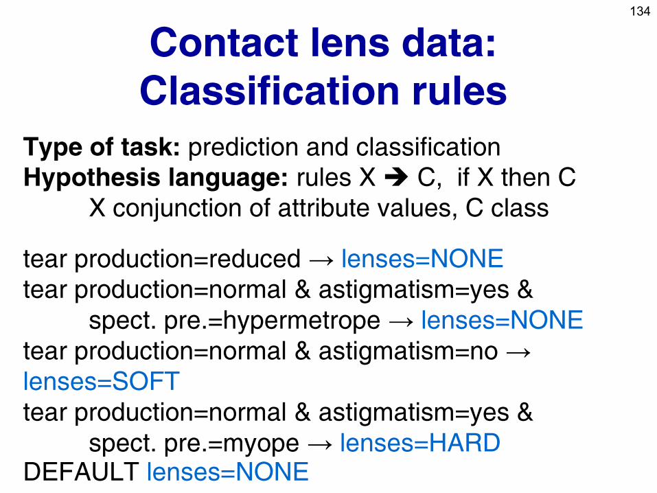
Contact lens data:
Classification rules
Type of task: prediction and classification
Hypothesis language: rules X C, if X then C X conjunction of attribute values, C class
tear production=reduced → lenses=NONE
tear production=normal & astigmatism=yes &
spect. pre.=hypermetrope → lenses=NONE
tear production=normal & astigmatism=no →
lenses=SOFT
tear production=normal & astigmatism=yes &
spect. pre.=myope → lenses=HARD DEFAULT lenses=NONE
135
Rule learning
• Two rule learning approaches:
– Learn decision tree, convert to rules
– Learn set/list of rules
• Learning an unordered set of rules
• Learning an ordered list of rules
• Heuristics, overfitting, pruning
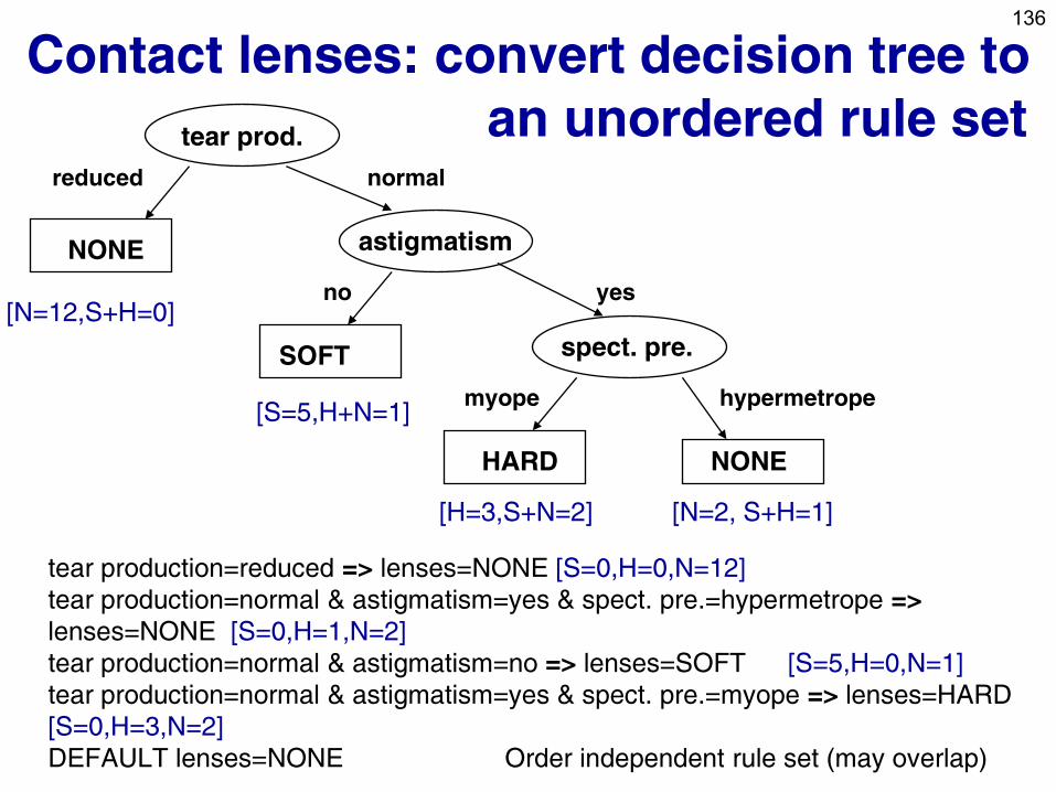
136
Contact lenses: convert decision tree to
an unordered rule set tear prod.
astigmatism
spect. pre.
NONE
NONE
reduced
no yes
normal
hypermetrope
SOFT
myope
HARD
[N=12,S+H=0]
[N=2, S+H=1]
[S=5,H+N=1]
[H=3,S+N=2]
tear production=reduced => lenses=NONE [S=0,H=0,N=12]
tear production=normal & astigmatism=yes & spect. pre.=hypermetrope =>
lenses=NONE [S=0,H=1,N=2]
tear production=normal & astigmatism=no => lenses=SOFT [S=5,H=0,N=1]
tear production=normal & astigmatism=yes & spect. pre.=myope => lenses=HARD
[S=0,H=3,N=2]
DEFAULT lenses=NONE Order independent rule set (may overlap)
137
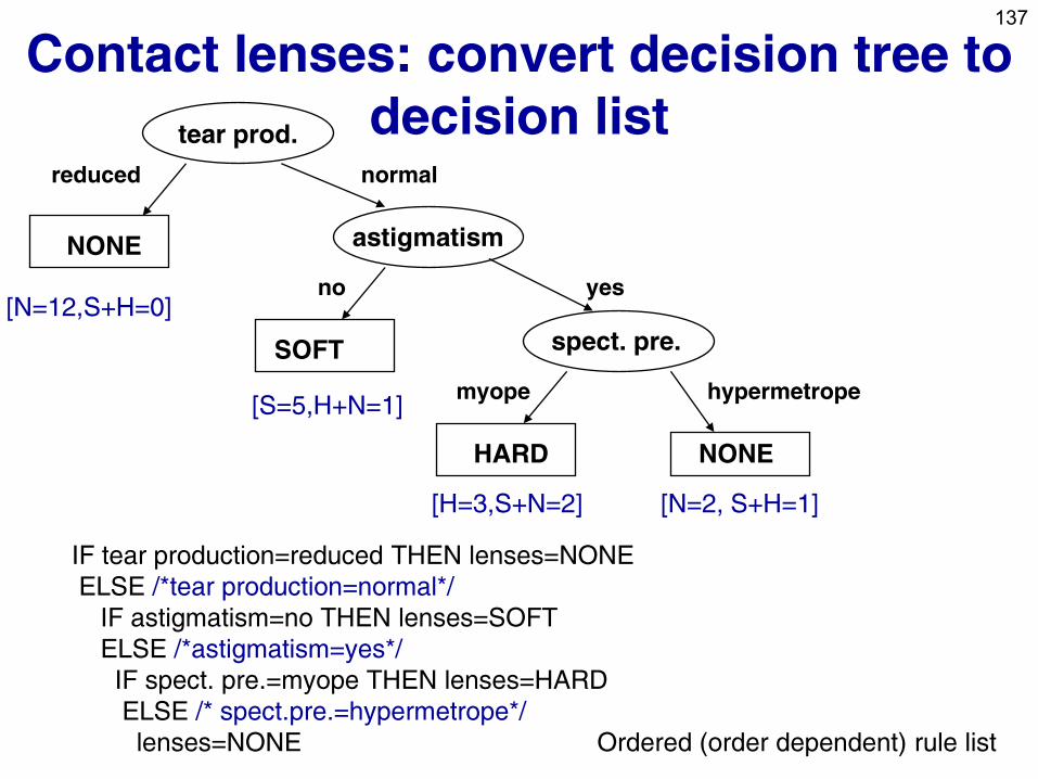
Contact lenses: convert decision tree to
decision list tear prod.
astigmatism
spect. pre.
NONE
NONE
reduced
no yes
normal
hypermetrope
SOFT
myope
HARD
[N=12,S+H=0]
[N=2, S+H=1]
[S=5,H+N=1]
[H=3,S+N=2]
IF tear production=reduced THEN lenses=NONE
ELSE /*tear production=normal*/
IF astigmatism=no THEN lenses=SOFT
ELSE /*astigmatism=yes*/
IF spect. pre.=myope THEN lenses=HARD
ELSE /* spect.pre.=hypermetrope*/
lenses=NONE Ordered (order dependent) rule list
138
Converting decision tree to rules, and
rule post-pruning (Quinlan 1993)
• Very frequently used method, e.g., in C4.5
and J48
• Procedure:
– grow a full tree (allowing overfitting)
– convert the tree to an equivalent set of rules
– prune each rule independently of others
– sort final rules into a desired sequence for use
139
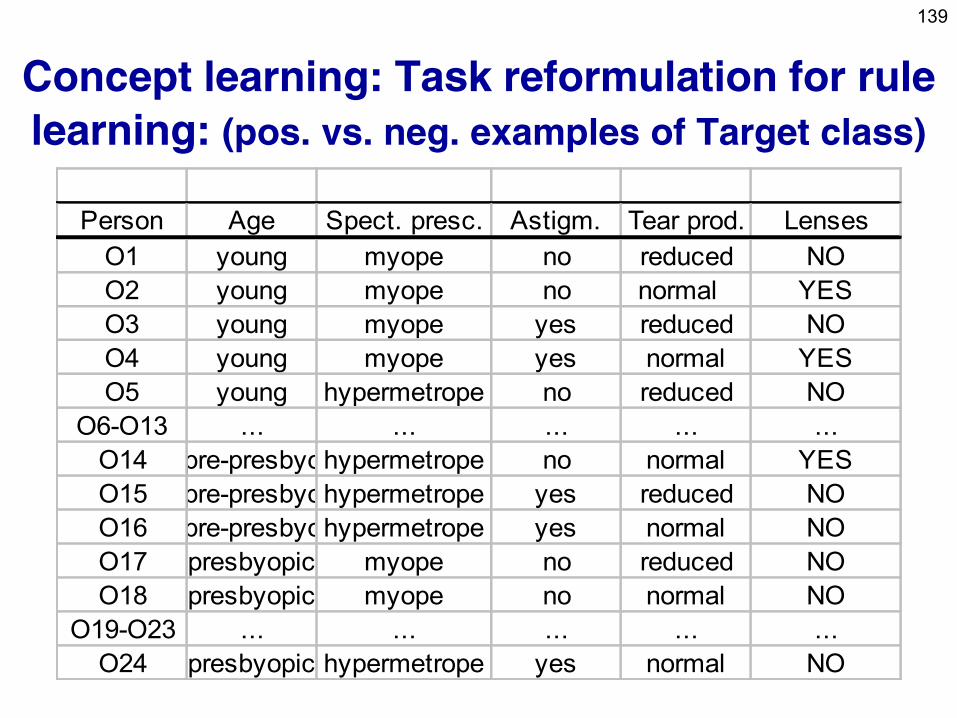
Concept learning: Task reformulation for rule
learning: (pos. vs. neg. examples of Target class)
Person Age Spect. presc. Astigm. Tear prod. Lenses
O1 young myope no reduced NO
O2 young myope no normal YES
O3 young myope yes reduced NO
O4 young myope yes normal YES
O5 young hypermetrope no reduced NO
O6-O13 ... ... ... ... ...
O14 pre-presbyohypermetrope no normal YES
O15 pre-presbyohypermetrope yes reduced NO
O16 pre-presbyohypermetrope yes normal NO
O17 presbyopic myope no reduced NO
O18 presbyopic myope no normal NO
O19-O23 ... ... ... ... ...
O24 presbyopic hypermetrope yes normal NO
140
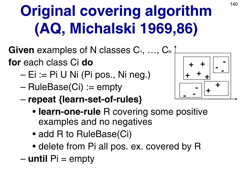
Original covering algorithm
(AQ, Michalski 1969,86)
Given examples of N classes C1, …, CN
for each class Ci do
– Ei := Pi U Ni (Pi pos., Ni neg.)
– RuleBase(Ci) := empty
– repeat {learn-set-of-rules}
• learn-one-rule R covering some positive examples and no negatives
• add R to RuleBase(Ci)
• delete from Pi all pos. ex. covered by R
– until Pi = empty
+ +
+
+ +
+ -
- -
- -
+ -
141
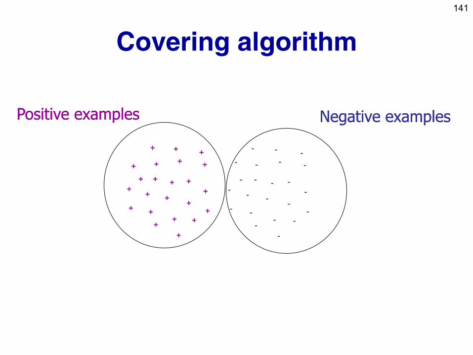
Covering algorithm
+ +
+
+
+
+
+
+
+
+ + +
+
+
+
+
+ +
+
+
+ +
+
- -
-
-
-
-
-
-
-
- -
-
-
-
-
- -
-
-
- -
-
Positive examplesPositive examples NNegative examplesegative examples
-

142
Covering algorithm
+ +
+
+
+
+
+
+
+
+ + +
+
+
+
+
+ +
+
+
+ +
+
- -
-
-
-
-
-
-
-
- -
-
-
-
-
- -
-
-
- -
-
Positive examplesPositive examples NNegative examplesegative examples
-
Rule1: Cl=+ Rule1: Cl=+ Cond2Cond2 AND Cond3AND Cond3
143
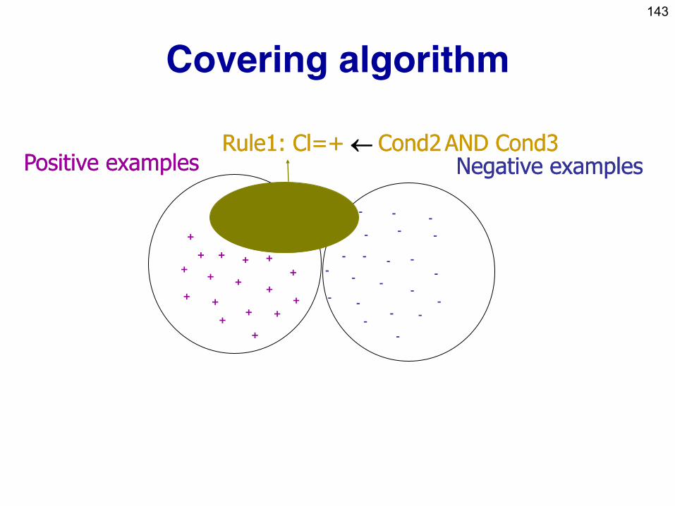
Covering algorithm
+
+
+
+
+
+
+
+
+
+
+ +
+
+
+ +
+
- -
-
-
-
-
-
-
-
- -
-
-
-
-
- -
-
-
- -
-
Positive examplesPositive examples NNegative examplesegative examples
-
Rule1: Cl=+ Rule1: Cl=+ Cond2Cond2 AND Cond3AND Cond3
144
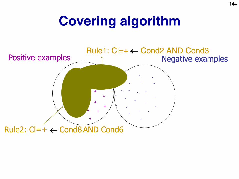
Covering algorithm
+
+
+
+
+
+
+
- -
-
-
-
-
-
-
-
- -
-
-
-
-
- -
-
-
- -
-
Positive examplesPositive examples NNegative examplesegative examples
-
Rule1: Cl=+ Rule1: Cl=+ Cond2 AND Cond3Cond2 AND Cond3
Rule2: Cl=+ Rule2: Cl=+ Cond8Cond8 AND Cond6AND Cond6

145
PlayGolf: Training examples
Day Outlook Temperature Humidity Wind PlayTennis
D1 Sunny Hot High Weak No
D2 Sunny Hot High Strong No
D3 Overcast Hot High Weak Yes
D4 Rain Mild High Weak Yes
D5 Rain Cool Normal Weak Yes
D6 Rain Cool Normal Strong No
D7 Overcast Cool Normal Strong Yes
D8 Sunny Mild High Weak No
D9 Sunny Cool Normal Weak Yes
D10 Rain Mild Normal Weak Yes
D11 Sunny Mild Normal Strong Yes
D12 Overcast Mild High Weak Yes
D13 Overcast Hot Normal Weak Yes
D14 Rain Mild High Strong No
146
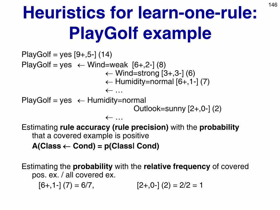
Heuristics for learn-one-rule:
PlayGolf example PlayGolf = yes [9+,5-] (14)
PlayGolf = yes Wind=weak [6+,2-] (8) Wind=strong [3+,3-] (6) Humidity=normal [6+,1-] (7) …
PlayGolf = yes Humidity=normal Outlook=sunny [2+,0-] (2) …
Estimating rule accuracy (rule precision) with the probability that a covered example is positive
A(Class Cond) = p(Class| Cond)
Estimating the probability with the relative frequency of covered pos. ex. / all covered ex.
[6+,1-] (7) = 6/7, [2+,0-] (2) = 2/2 = 1

147
Probability estimates
• Relative frequency : – problems with small samples
• Laplace estimate : – assumes uniform prior
distribution of k classes
)(
).(
)|(
Condn
CondClassn
CondClassp
kCondn
CondClassn
)(
1).(2k
[6+,1-] (7) = 6/7
[2+,0-] (2) = 2/2 = 1
[6+,1-] (7) = 6+1 / 7+2 = 7/9
[2+,0-] (2) = 2+1 / 2+2 = 3/4
148
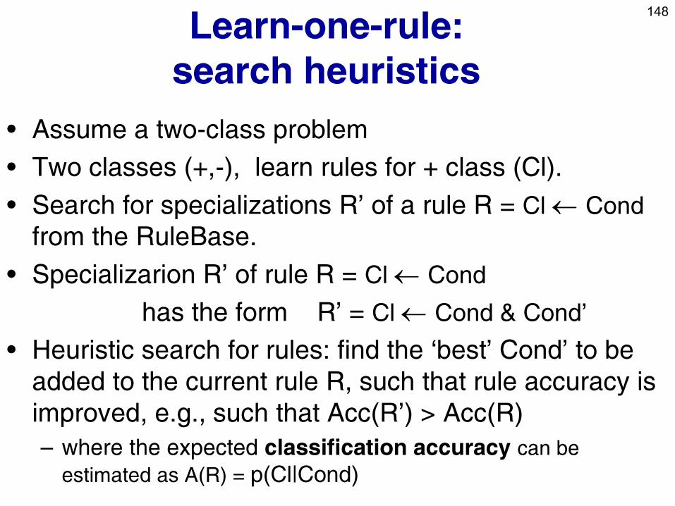
Learn-one-rule:
search heuristics
• Assume a two-class problem
• Two classes (+,-), learn rules for + class (Cl).
• Search for specializations R’ of a rule R = Cl Cond
from the RuleBase.
• Specializarion R’ of rule R = Cl Cond
has the form R’ = Cl Cond & Cond’
• Heuristic search for rules: find the ‘best’ Cond’ to be
added to the current rule R, such that rule accuracy is
improved, e.g., such that Acc(R’) > Acc(R)
– where the expected classification accuracy can be
estimated as A(R) = p(Cl|Cond)
149
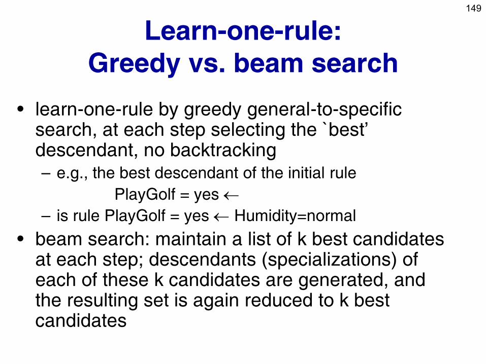
Learn-one-rule:
Greedy vs. beam search
• learn-one-rule by greedy general-to-specific search, at each step selecting the `best’ descendant, no backtracking – e.g., the best descendant of the initial rule
PlayGolf = yes
– is rule PlayGolf = yes Humidity=normal
• beam search: maintain a list of k best candidates at each step; descendants (specializations) of each of these k candidates are generated, and the resulting set is again reduced to k best candidates
150
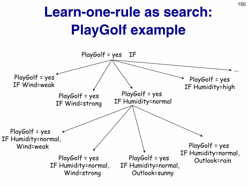
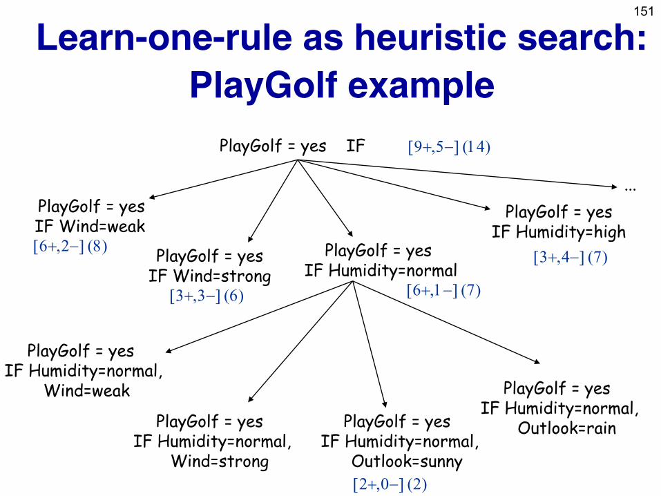
Learn-one-rule as search:
PlayGolf example
PlayGolf = yes IF
PlayGolf = yes IF Wind=weak
PlayGolf = yes IF Wind=strong
PlayGolf = yes IF Humidity=normal
PlayGolf = yes IF Humidity=high
PlayGolf = yes IF Humidity=normal,
Wind=weak
PlayGolf = yes IF Humidity=normal,
Wind=strong
PlayGolf = yes IF Humidity=normal,
Outlook=sunny
PlayGolf = yes IF Humidity=normal,
Outlook=rain
...
151
Learn-one-rule as heuristic search:
PlayGolf example
PlayGolf = yes IF
PlayGolf = yes IF Wind=weak
PlayGolf = yes IF Wind=strong
PlayGolf = yes IF Humidity=normal
PlayGolf = yes IF Humidity=high
PlayGolf = yes IF Humidity=normal,
Wind=weak
PlayGolf = yes IF Humidity=normal,
Wind=strong
PlayGolf = yes IF Humidity=normal,
Outlook=sunny
PlayGolf = yes IF Humidity=normal,
Outlook=rain
[9,5] (14)
[6,2] (8)
[3,3] (6) [6,1] (7)
[3,4] (7)
...
[2,0] (2)
152
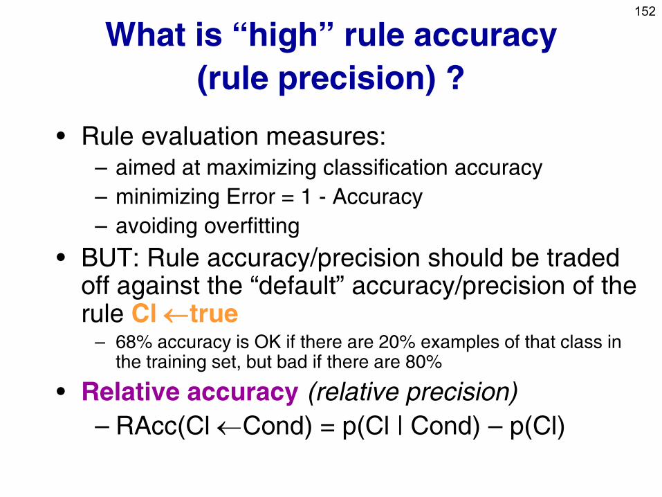
What is “high” rule accuracy
(rule precision) ?
• Rule evaluation measures: – aimed at maximizing classification accuracy
– minimizing Error = 1 - Accuracy
– avoiding overfitting
• BUT: Rule accuracy/precision should be traded off against the “default” accuracy/precision of the rule Cl true
– 68% accuracy is OK if there are 20% examples of that class in the training set, but bad if there are 80%
• Relative accuracy (relative precision)
– RAcc(Cl Cond) = p(Cl | Cond) – p(Cl)
153
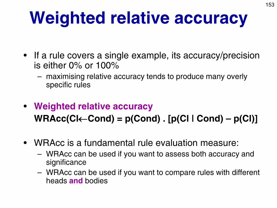
Weighted relative accuracy
• If a rule covers a single example, its accuracy/precision is either 0% or 100% – maximising relative accuracy tends to produce many overly
specific rules
• Weighted relative accuracy
WRAcc(ClCond) = p(Cond) . [p(Cl | Cond) – p(Cl)]
• WRAcc is a fundamental rule evaluation measure: – WRAcc can be used if you want to assess both accuracy and
significance
– WRAcc can be used if you want to compare rules with different heads and bodies
154
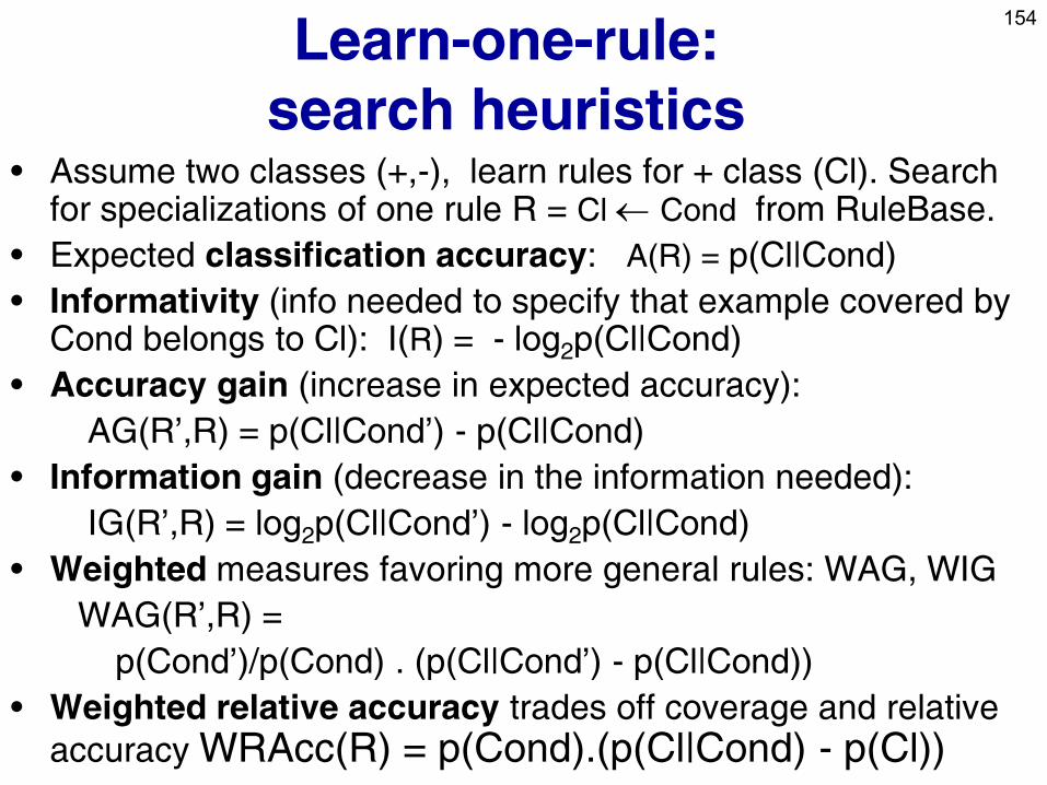
Learn-one-rule:
search heuristics • Assume two classes (+,-), learn rules for + class (Cl). Search
for specializations of one rule R = Cl Cond from RuleBase.
• Expected classification accuracy: A(R) = p(Cl|Cond)
• Informativity (info needed to specify that example covered by Cond belongs to Cl): I(R) = - log2p(Cl|Cond)
• Accuracy gain (increase in expected accuracy):
AG(R’,R) = p(Cl|Cond’) - p(Cl|Cond)
• Information gain (decrease in the information needed):
IG(R’,R) = log2p(Cl|Cond’) - log2p(Cl|Cond)
• Weighted measures favoring more general rules: WAG, WIG
WAG(R’,R) =
p(Cond’)/p(Cond) . (p(Cl|Cond’) - p(Cl|Cond))
• Weighted relative accuracy trades off coverage and relative
accuracy WRAcc(R) = p(Cond).(p(Cl|Cond) - p(Cl))
155
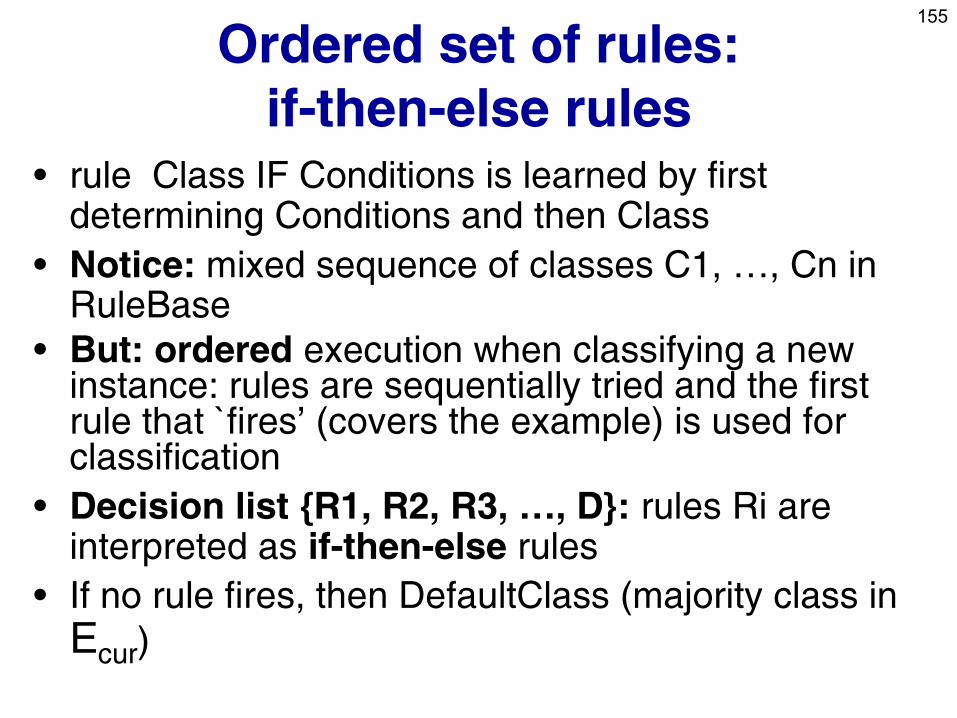
Ordered set of rules:
if-then-else rules • rule Class IF Conditions is learned by first
determining Conditions and then Class
• Notice: mixed sequence of classes C1, …, Cn in RuleBase
• But: ordered execution when classifying a new instance: rules are sequentially tried and the first rule that `fires’ (covers the example) is used for classification
• Decision list {R1, R2, R3, …, D}: rules Ri are interpreted as if-then-else rules
• If no rule fires, then DefaultClass (majority class in
Ecur)
156
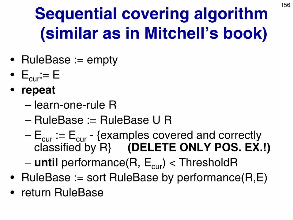
Sequential covering algorithm
(similar as in Mitchell’s book)
• RuleBase := empty
• Ecur:= E
• repeat
– learn-one-rule R
– RuleBase := RuleBase U R
– Ecur := Ecur - {examples covered and correctly classified by R} (DELETE ONLY POS. EX.!)
– until performance(R, Ecur) < ThresholdR
• RuleBase := sort RuleBase by performance(R,E)
• return RuleBase
157
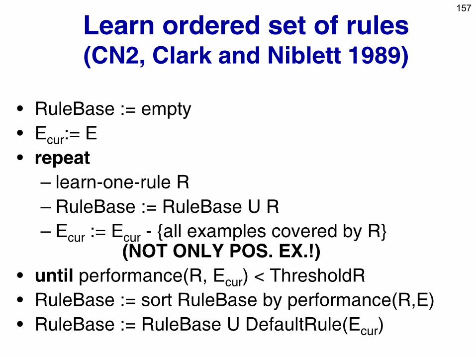
Learn ordered set of rules (CN2, Clark and Niblett 1989)
• RuleBase := empty
• Ecur:= E
• repeat
– learn-one-rule R
– RuleBase := RuleBase U R
– Ecur := Ecur - {all examples covered by R} (NOT ONLY POS. EX.!)
• until performance(R, Ecur) < ThresholdR
• RuleBase := sort RuleBase by performance(R,E)
• RuleBase := RuleBase U DefaultRule(Ecur)
158
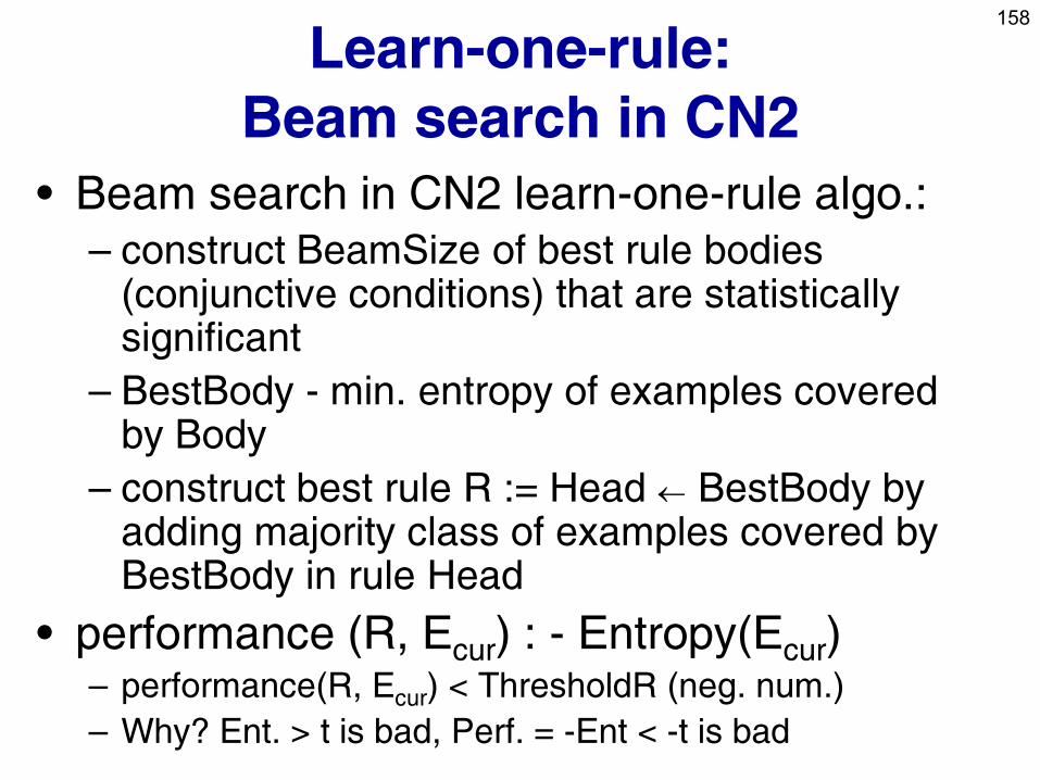
Learn-one-rule:
Beam search in CN2
• Beam search in CN2 learn-one-rule algo.:
– construct BeamSize of best rule bodies (conjunctive conditions) that are statistically significant
– BestBody - min. entropy of examples covered by Body
– construct best rule R := Head BestBody by adding majority class of examples covered by BestBody in rule Head
• performance (R, Ecur) : - Entropy(Ecur) – performance(R, Ecur) < ThresholdR (neg. num.)
– Why? Ent. > t is bad, Perf. = -Ent < -t is bad
159
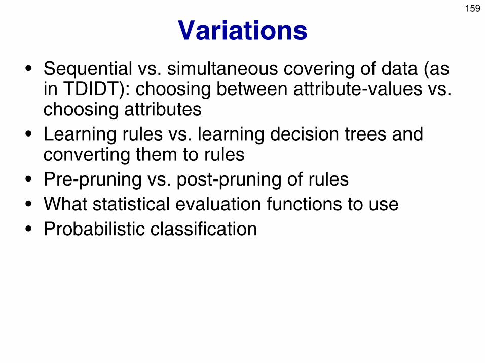
Variations
• Sequential vs. simultaneous covering of data (as in TDIDT): choosing between attribute-values vs. choosing attributes
• Learning rules vs. learning decision trees and converting them to rules
• Pre-pruning vs. post-pruning of rules
• What statistical evaluation functions to use
• Probabilistic classification
160
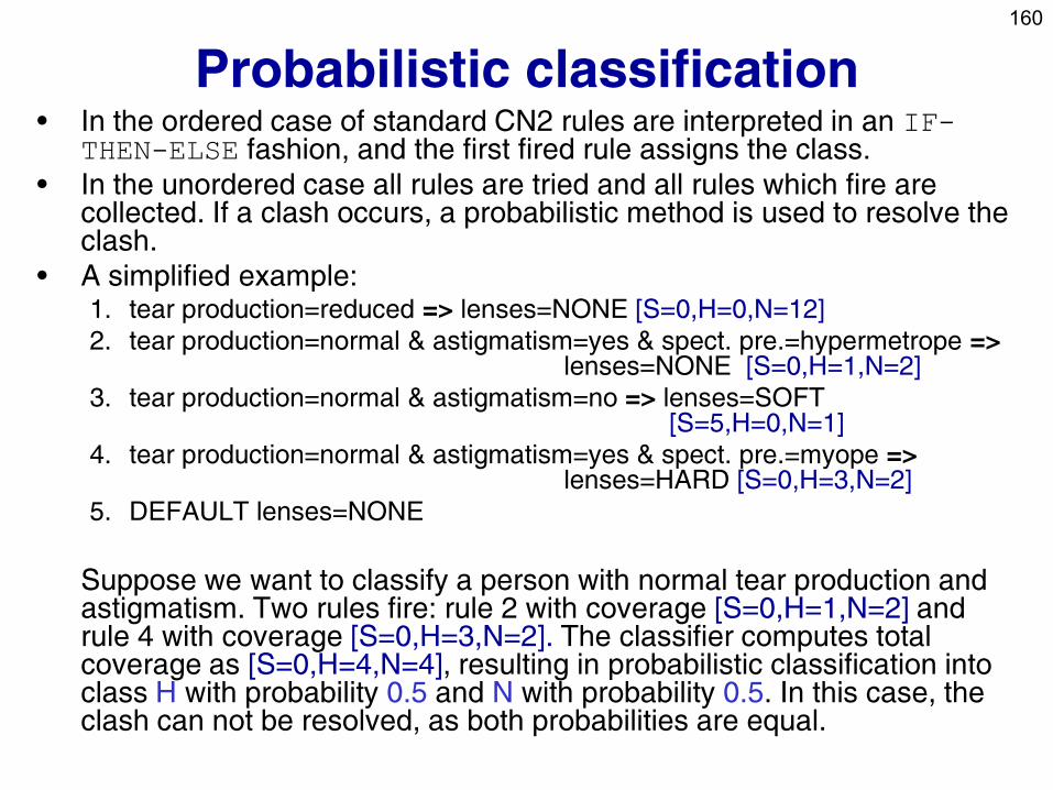
Probabilistic classification • In the ordered case of standard CN2 rules are interpreted in an IF-
THEN-ELSE fashion, and the first fired rule assigns the class.
• In the unordered case all rules are tried and all rules which fire are collected. If a clash occurs, a probabilistic method is used to resolve the clash.
• A simplified example: 1. tear production=reduced => lenses=NONE [S=0,H=0,N=12]
2. tear production=normal & astigmatism=yes & spect. pre.=hypermetrope => lenses=NONE [S=0,H=1,N=2]
3. tear production=normal & astigmatism=no => lenses=SOFT [S=5,H=0,N=1]
4. tear production=normal & astigmatism=yes & spect. pre.=myope => lenses=HARD [S=0,H=3,N=2]
5. DEFAULT lenses=NONE
Suppose we want to classify a person with normal tear production and astigmatism. Two rules fire: rule 2 with coverage [S=0,H=1,N=2] and rule 4 with coverage [S=0,H=3,N=2]. The classifier computes total coverage as [S=0,H=4,N=4], resulting in probabilistic classification into class H with probability 0.5 and N with probability 0.5. In this case, the clash can not be resolved, as both probabilities are equal.
161
Part II. Predictive DM techniques
• Naïve Bayesian classifier
• Decision tree learning
• Classification rule learning
• Classifier evaluation
162
Classifier evaluation
• Accuracy and Error
• n-fold cross-validation
• Confusion matrix
• ROC
163
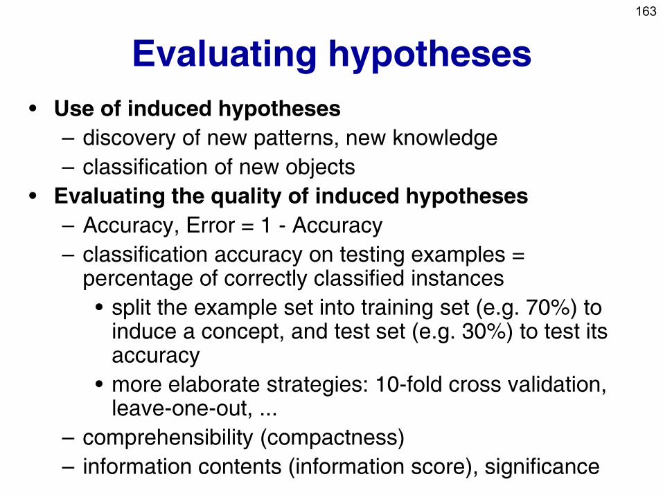
Evaluating hypotheses
• Use of induced hypotheses
– discovery of new patterns, new knowledge
– classification of new objects
• Evaluating the quality of induced hypotheses
– Accuracy, Error = 1 - Accuracy
– classification accuracy on testing examples = percentage of correctly classified instances
• split the example set into training set (e.g. 70%) to induce a concept, and test set (e.g. 30%) to test its accuracy
• more elaborate strategies: 10-fold cross validation, leave-one-out, ...
– comprehensibility (compactness)
– information contents (information score), significance
164
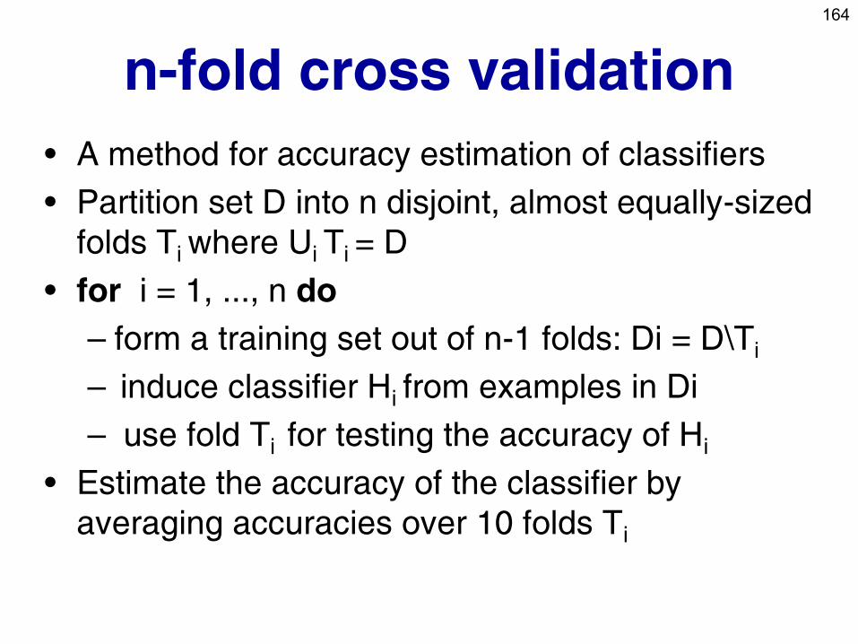
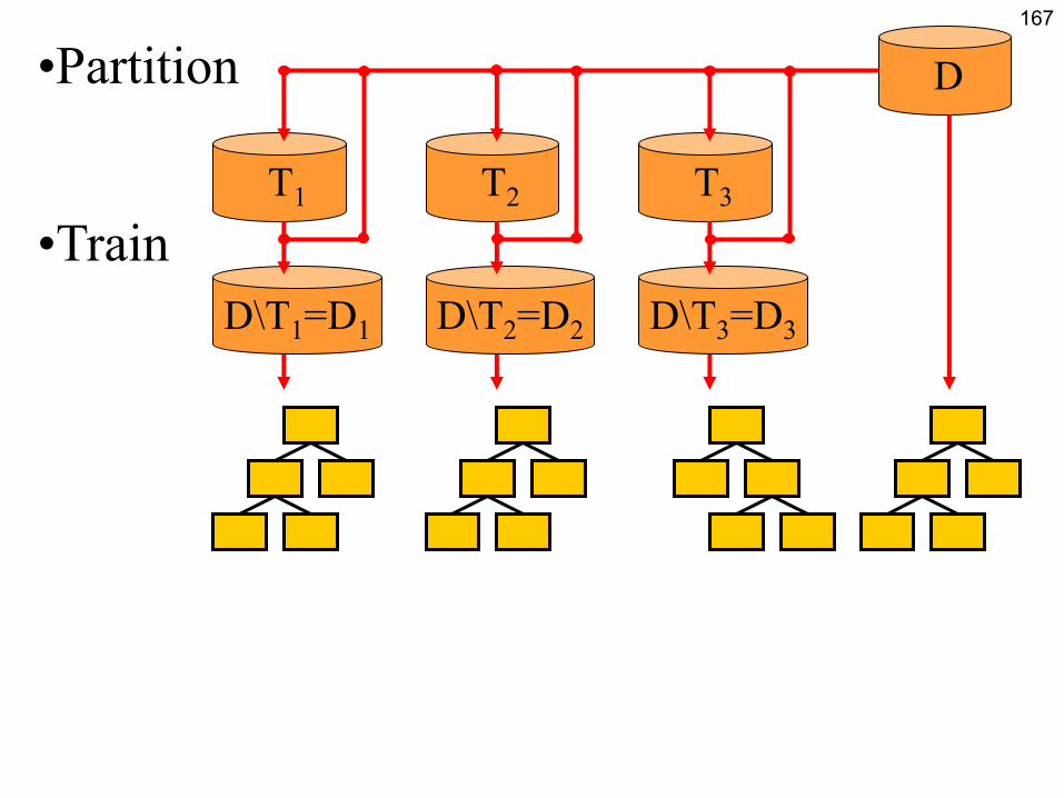
n-fold cross validation
• A method for accuracy estimation of classifiers
• Partition set D into n disjoint, almost equally-sized
folds Ti where Ui Ti = D
• for i = 1, ..., n do
– form a training set out of n-1 folds: Di = D\Ti
– induce classifier Hi from examples in Di
– use fold Ti for testing the accuracy of Hi
• Estimate the accuracy of the classifier by
averaging accuracies over 10 folds Ti
165
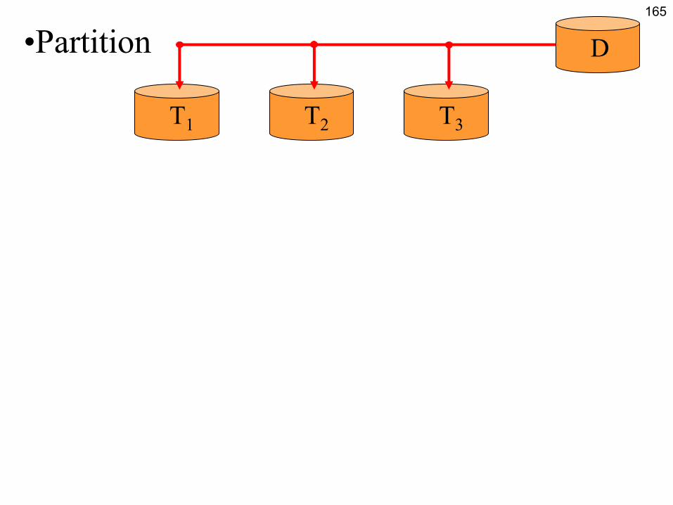
•Partition D
T1 T2 T3
166
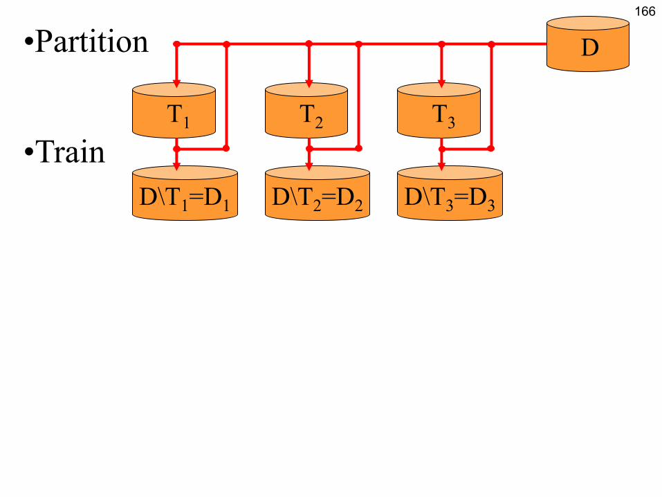
•Partition
•Train
D\T1=D1 D\T2=D2 D\T3=D3
D
T1 T2 T3
167
•Partition
•Train
D\T1=D1 D\T2=D2 D\T3=D3
D
T1 T2 T3
168
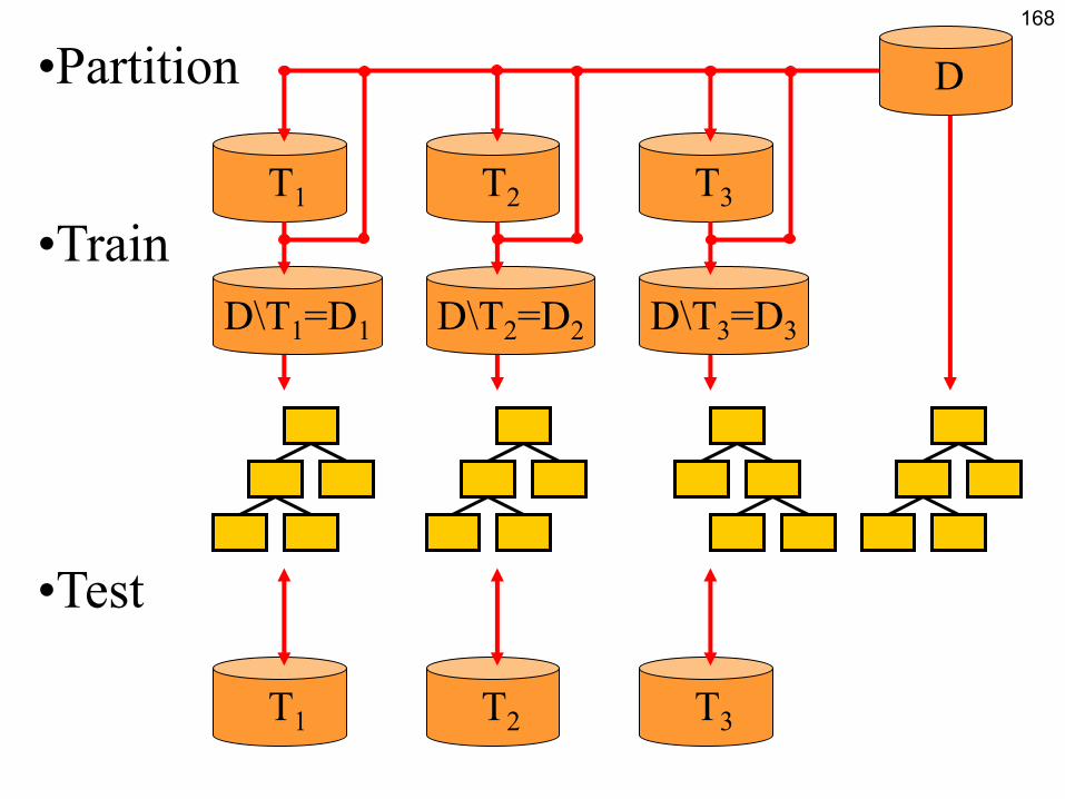
•Partition
•Train
•Test
D\T1=D1 D\T2=D2 D\T3=D3
D
T1 T2 T3
T1 T2 T3
169
Confusion matrix and
rule (in)accuracy
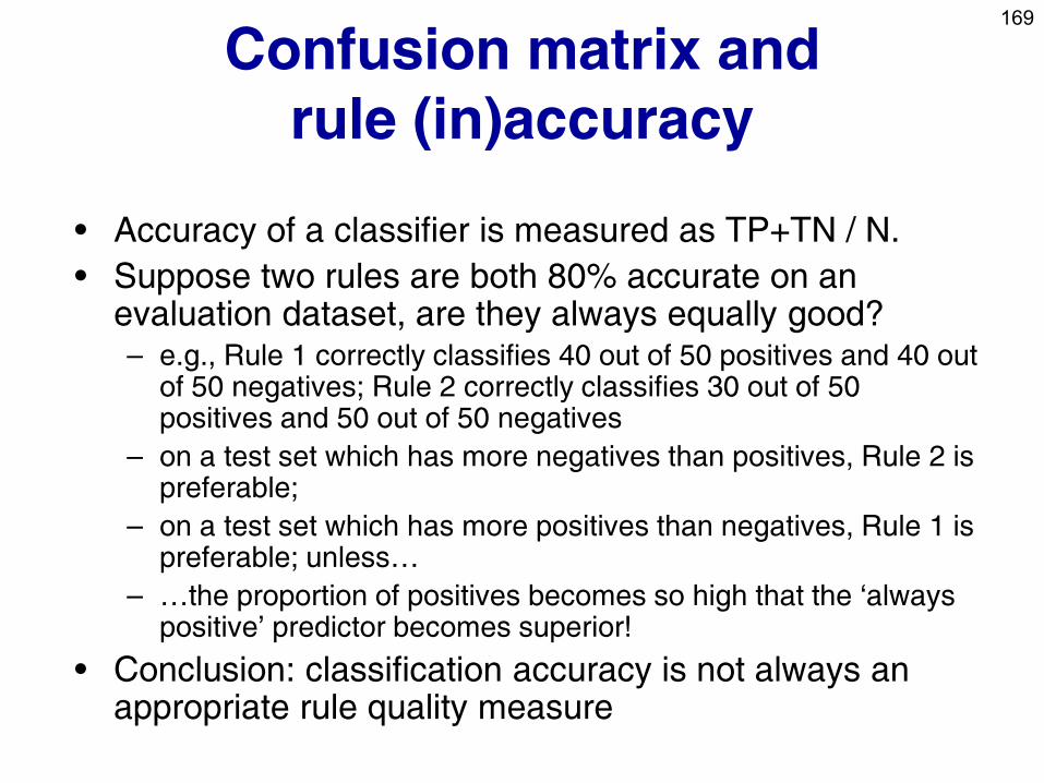
• Accuracy of a classifier is measured as TP+TN / N.
• Suppose two rules are both 80% accurate on an evaluation dataset, are they always equally good? – e.g., Rule 1 correctly classifies 40 out of 50 positives and 40 out
of 50 negatives; Rule 2 correctly classifies 30 out of 50 positives and 50 out of 50 negatives
– on a test set which has more negatives than positives, Rule 2 is preferable;
– on a test set which has more positives than negatives, Rule 1 is preferable; unless…
– …the proportion of positives becomes so high that the ‘always positive’ predictor becomes superior!
• Conclusion: classification accuracy is not always an appropriate rule quality measure

170
Confusion matrix
• also called contingency table
Classifier 1 Predicted positive Predicted negative
Positive examples 40 10 50 Negative examples 10 40 50 50 50 100
Classifier 2 Predicted positive Predicted negative
Positive examples 30 20 50 Negative examples 0 50 50 30 70 100
171
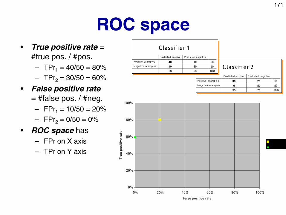
ROC space • True positive rate =
#true pos. / #pos.
– TPr1 = 40/50 = 80%
– TPr2 = 30/50 = 60%
• False positive rate
= #false pos. / #neg.
– FPr1 = 10/50 = 20%
– FPr2 = 0/50 = 0%
• ROC space has
– FPr on X axis
– TPr on Y axis
0%
20%
40%
60%
80%
100%
0% 20% 40% 60% 80% 100%
False posit ive rate
Tru
e p
osit
ive r
ate
classif ier 1
classif ier 2
Classifi er 2
Pred ic ted pos iti ve Pred ic ted nega tive
Pos iti ve exam ples 30 20 50
N ega tive ex am ples 0 50 50
30 70 10 0
Classifi er 1
Pred ic ted pos iti ve Pred ic ted nega tive
Pos iti ve exam ples 40 10 50
N ega tive ex am ples 10 40 50
50 50 10 0
172
0%
20%
40%
60%
80%
100%
0% 20% 40% 60% 80% 100%
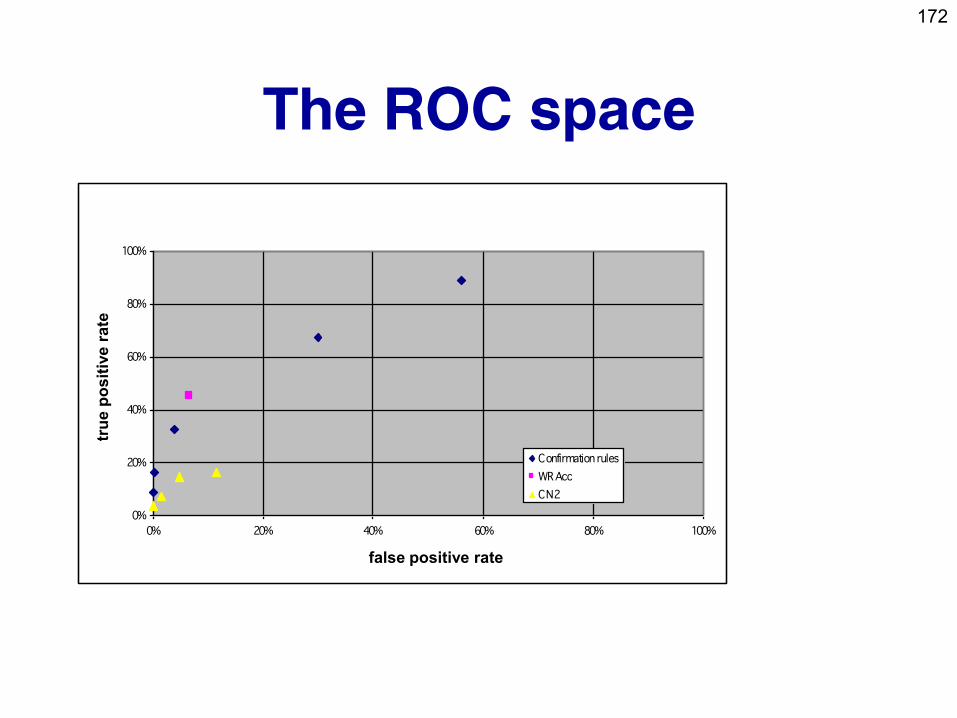
Confirmation rules
WRAcc
CN2
false positive rate
tru
e p
osit
ive
ra
te
The ROC space
173
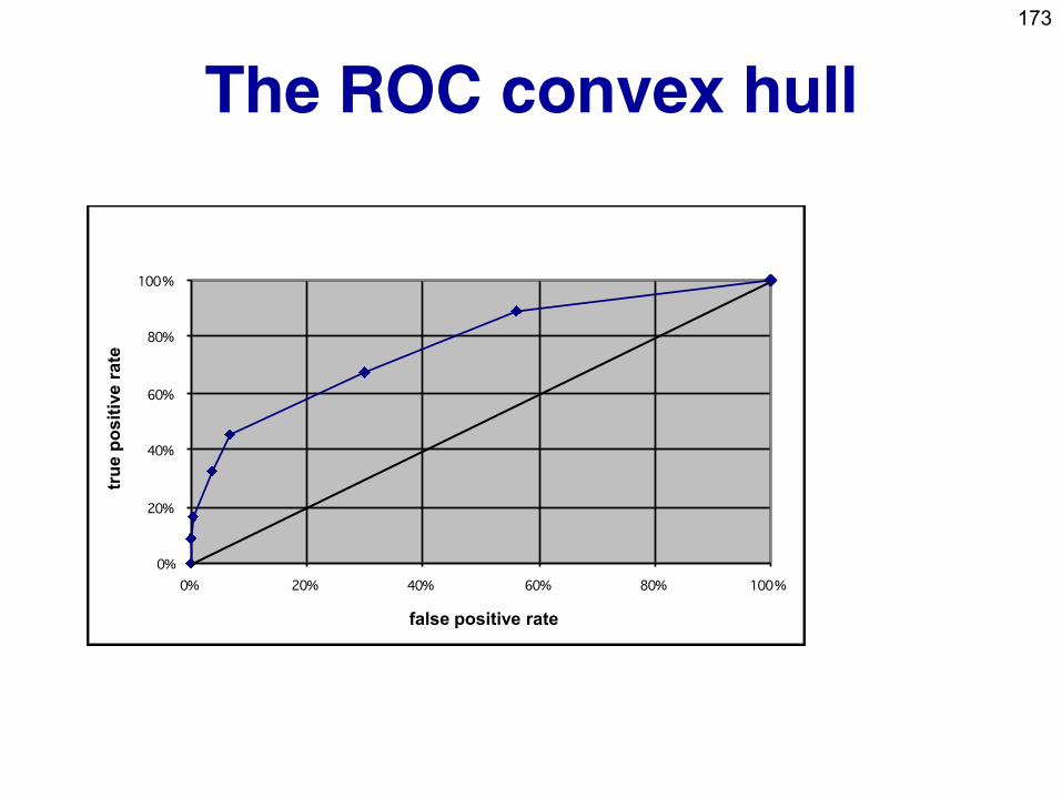
The ROC convex hull
0%
20%
40%
60%
80%
100%
0% 20% 40% 60% 80% 100%
false positive rate
tru
e p
osit
ive
ra
te
174
Summary of evaluation
• 10-fold cross-validation is a standard classifier
evaluation method used in machine learning
• ROC analysis is very natural for rule learning
and subgroup discovery
– can take costs into account
– here used for evaluation
– also possible to use as search heuristic
175
Part III. Numeric prediction
• Baseline
• Linear Regression
• Regression tree
• Model Tree
• kNN
176
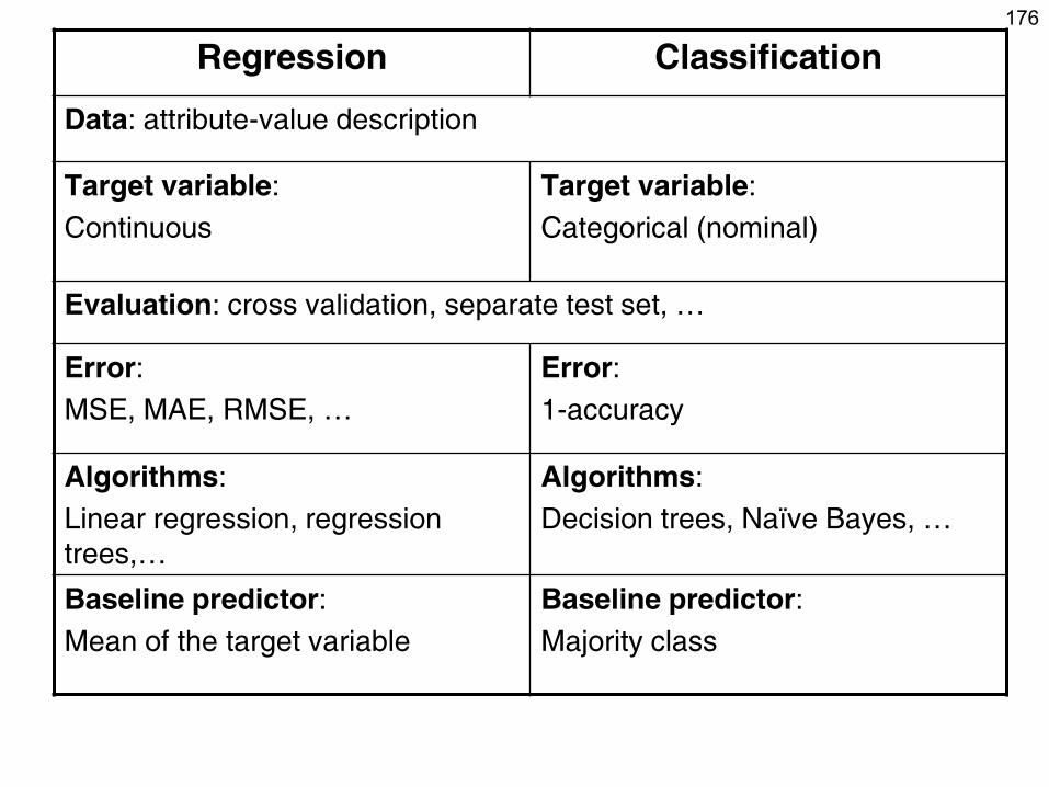
Regression Classification
Data: attribute-value description
Target variable:
Continuous
Target variable:
Categorical (nominal)
Evaluation: cross validation, separate test set, …
Error:
MSE, MAE, RMSE, …
Error:
1-accuracy
Algorithms:
Linear regression, regression
trees,…
Algorithms:
Decision trees, Naïve Bayes, …
Baseline predictor:
Mean of the target variable
Baseline predictor:
Majority class
177
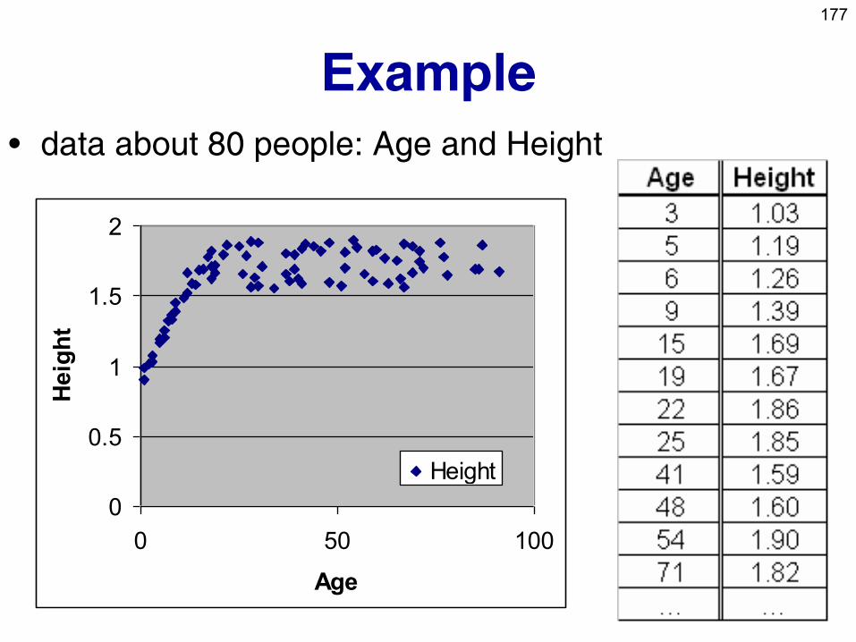
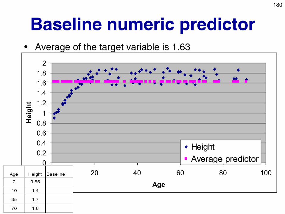
Example
• data about 80 people: Age and Height
0
0.5
1
1.5
2
0 50 100
Age
Heig
ht
Height
178
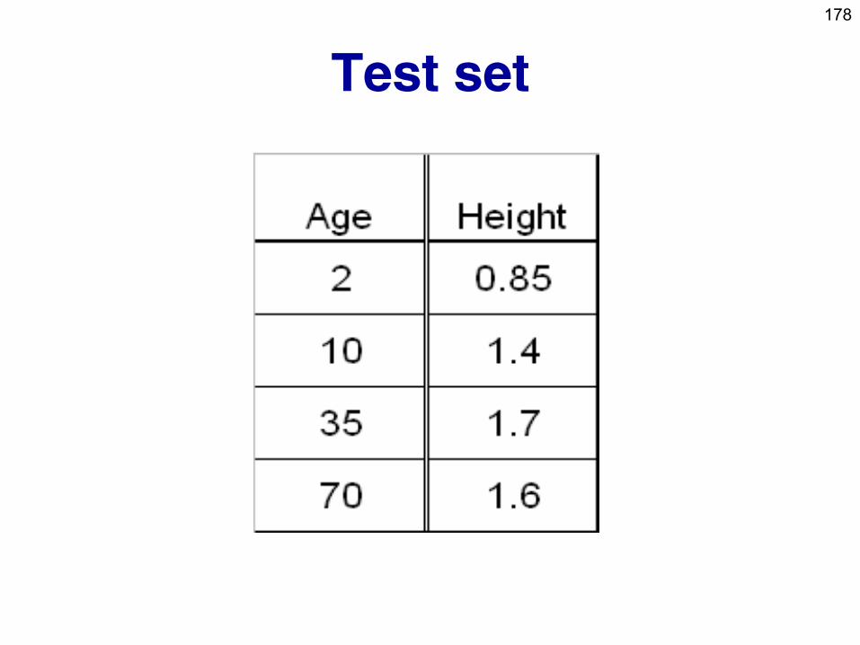
Test set
179
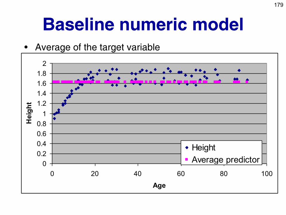
Baseline numeric model • Average of the target variable
0
0.2
0.4
0.6
0.8
1
1.2
1.4
1.6
1.8
2
0 20 40 60 80 100
Age
He
igh
t
Height
Average predictor
180
Baseline numeric predictor • Average of the target variable is 1.63
0
0.2
0.4
0.6
0.8
1
1.2
1.4
1.6
1.8
2
0 20 40 60 80 100
Age
He
igh
t
Height
Average predictor
181
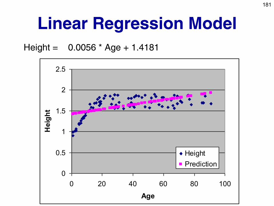
Linear Regression Model
Height = 0.0056 * Age + 1.4181
0
0.5
1
1.5
2
2.5
0 20 40 60 80 100
Age
He
igh
t
Height
Prediction
182
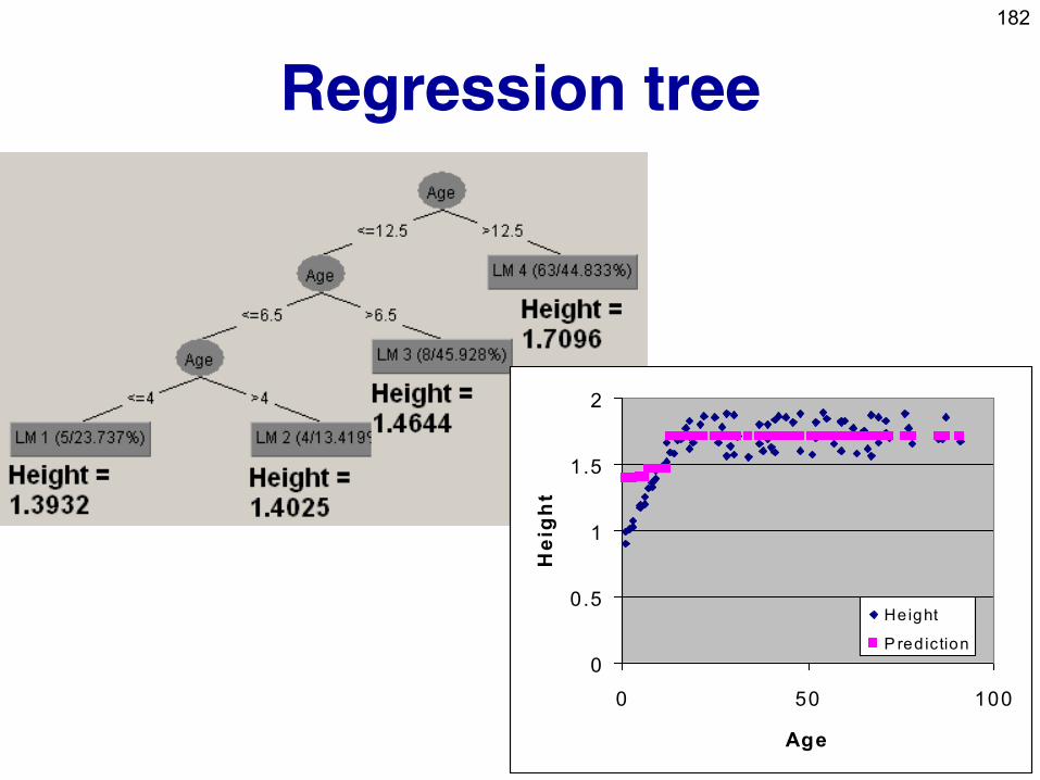
Regression tree
0
0.5
1
1.5
2
0 50 100
Age
He
igh
t
Height
P red iction
183
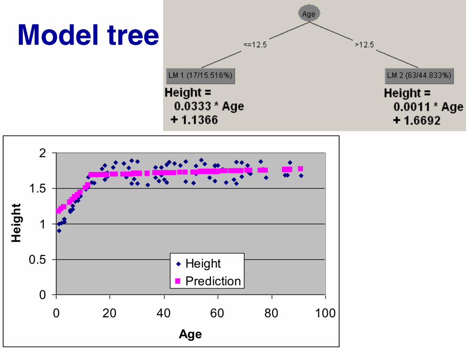
Model tree
0
0.5
1
1.5
2
0 20 40 60 80 100
Age
He
igh
t
Height
Prediction
184
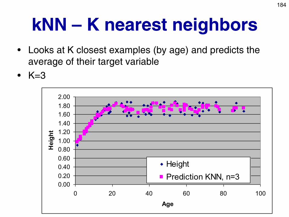
kNN – K nearest neighbors
• Looks at K closest examples (by age) and predicts the
average of their target variable
• K=3
0.00
0.20
0.40
0.60
0.80
1.00
1.20
1.40
1.60
1.80
2.00
0 20 40 60 80 100
Age
He
igh
t
Height
Prediction KNN, n=3
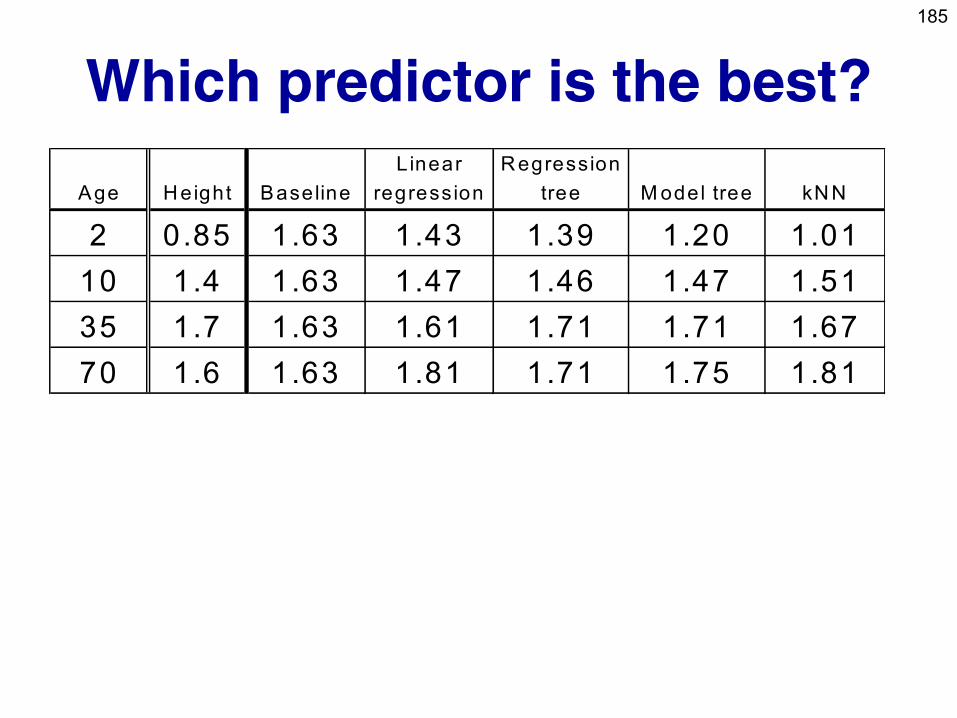
185
Which predictor is the best?
Age Height Baseline
Linear
regression
Regression
tree M odel tree kNN
2 0.85 1.63 1.43 1.39 1.20 1.01
10 1.4 1.63 1.47 1.46 1.47 1.51
35 1.7 1.63 1.61 1.71 1.71 1.67
70 1.6 1.63 1.81 1.71 1.75 1.81
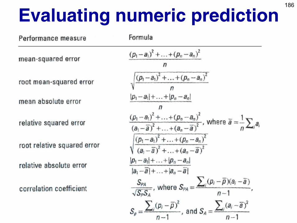
186
Evaluating numeric prediction
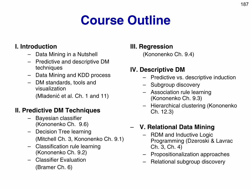
187
Course Outline
I. Introduction
– Data Mining in a Nutshell
– Predictive and descriptive DM techniques
– Data Mining and KDD process
– DM standards, tools and visualization
(Mladenić et al. Ch. 1 and 11)
II. Predictive DM Techniques
– Bayesian classifier (Kononenko Ch. 9.6)
– Decision Tree learning
(Mitchell Ch. 3, Kononenko Ch. 9.1)
– Classification rule learning (Kononenko Ch. 9.2)
– Classifier Evaluation
(Bramer Ch. 6)
III. Regression
(Kononenko Ch. 9.4)
IV. Descriptive DM
– Predictive vs. descriptive induction
– Subgroup discovery
– Association rule learning (Kononenko Ch. 9.3)
– Hierarchical clustering (Kononenko Ch. 12.3)
– V. Relational Data Mining
– RDM and Inductive Logic Programming (Dzeroski & Lavrac Ch. 3, Ch. 4)
– Propositionalization approaches
– Relational subgroup discovery
188
Part IV. Descriptive DM techniques
• Predictive vs. descriptive induction
• Subgroup discovery
• Association rule learning
• Hierarchical clustering
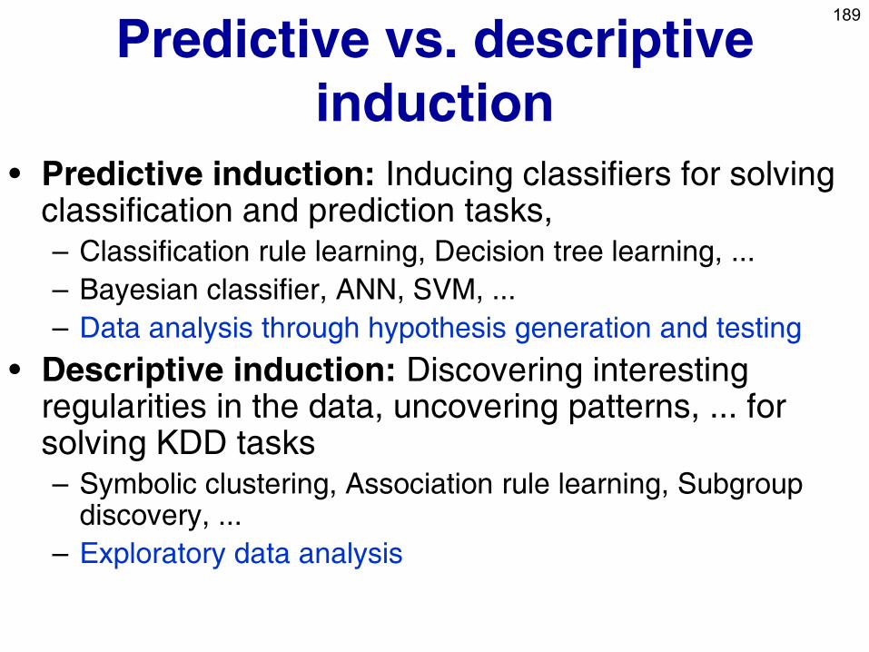
189
Predictive vs. descriptive
induction
• Predictive induction: Inducing classifiers for solving classification and prediction tasks, – Classification rule learning, Decision tree learning, ...
– Bayesian classifier, ANN, SVM, ...
– Data analysis through hypothesis generation and testing
• Descriptive induction: Discovering interesting regularities in the data, uncovering patterns, ... for solving KDD tasks – Symbolic clustering, Association rule learning, Subgroup
discovery, ...
– Exploratory data analysis
190
Descriptive DM
• Often used for preliminary explanatory data
analysis
• User gets feel for the data and its structure
• Aims at deriving descriptions of characteristics
of the data
• Visualization and descriptive statistical
techniques can be used
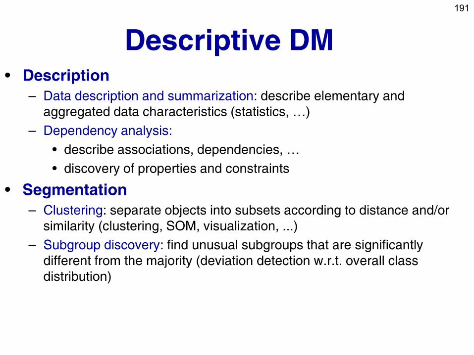
191
Descriptive DM • Description
– Data description and summarization: describe elementary and
aggregated data characteristics (statistics, …)
– Dependency analysis:
• describe associations, dependencies, …
• discovery of properties and constraints
• Segmentation
– Clustering: separate objects into subsets according to distance and/or
similarity (clustering, SOM, visualization, ...)
– Subgroup discovery: find unusual subgroups that are significantly
different from the majority (deviation detection w.r.t. overall class
distribution)
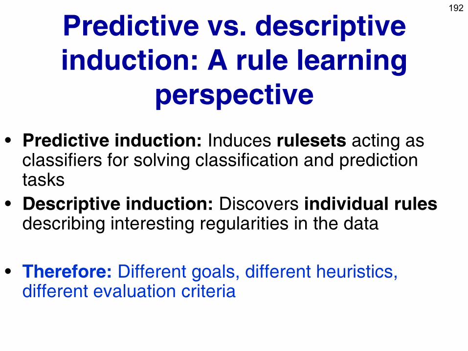
192
Predictive vs. descriptive
induction: A rule learning
perspective
• Predictive induction: Induces rulesets acting as classifiers for solving classification and prediction tasks
• Descriptive induction: Discovers individual rules describing interesting regularities in the data
• Therefore: Different goals, different heuristics, different evaluation criteria
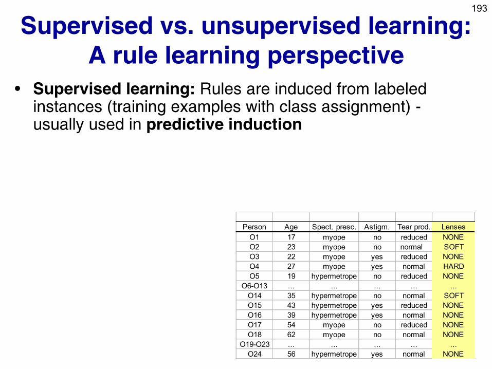
193
Supervised vs. unsupervised learning:
A rule learning perspective
• Supervised learning: Rules are induced from labeled instances (training examples with class assignment) - usually used in predictive induction
Person Age Spect. presc. Astigm. Tear prod. Lenses
O1 17 myope no reduced NONE
O2 23 myope no normal SOFT
O3 22 myope yes reduced NONE
O4 27 myope yes normal HARD
O5 19 hypermetrope no reduced NONE
O6-O13 ... ... ... ... ...
O14 35 hypermetrope no normal SOFT
O15 43 hypermetrope yes reduced NONE
O16 39 hypermetrope yes normal NONE
O17 54 myope no reduced NONE
O18 62 myope no normal NONE
O19-O23 ... ... ... ... ...
O24 56 hypermetrope yes normal NONE
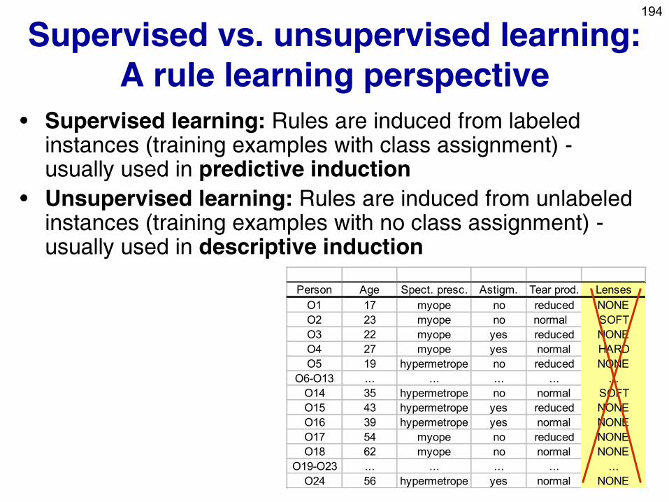
194
Supervised vs. unsupervised learning:
A rule learning perspective
• Supervised learning: Rules are induced from labeled instances (training examples with class assignment) - usually used in predictive induction
• Unsupervised learning: Rules are induced from unlabeled instances (training examples with no class assignment) - usually used in descriptive induction
Person Age Spect. presc. Astigm. Tear prod. Lenses
O1 17 myope no reduced NONE
O2 23 myope no normal SOFT
O3 22 myope yes reduced NONE
O4 27 myope yes normal HARD
O5 19 hypermetrope no reduced NONE
O6-O13 ... ... ... ... ...
O14 35 hypermetrope no normal SOFT
O15 43 hypermetrope yes reduced NONE
O16 39 hypermetrope yes normal NONE
O17 54 myope no reduced NONE
O18 62 myope no normal NONE
O19-O23 ... ... ... ... ...
O24 56 hypermetrope yes normal NONE
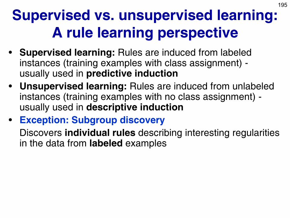
195
Supervised vs. unsupervised learning:
A rule learning perspective
• Supervised learning: Rules are induced from labeled instances (training examples with class assignment) - usually used in predictive induction
• Unsupervised learning: Rules are induced from unlabeled instances (training examples with no class assignment) - usually used in descriptive induction
• Exception: Subgroup discovery
Discovers individual rules describing interesting regularities in the data from labeled examples
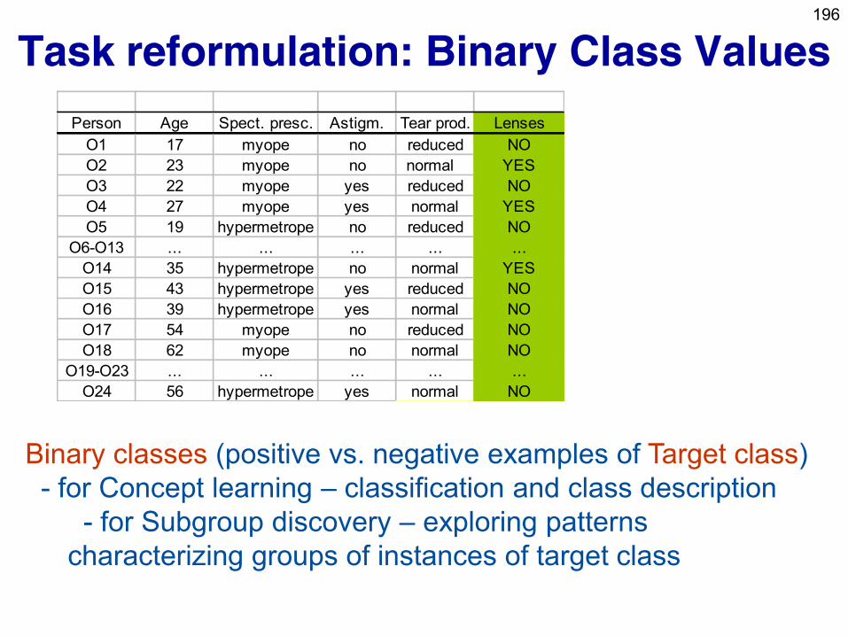
196
Task reformulation: Binary Class Values
Binary classes (positive vs. negative examples of Target class)
- for Concept learning – classification and class description
- for Subgroup discovery – exploring patterns
characterizing groups of instances of target class
Person Age Spect. presc. Astigm. Tear prod. Lenses
O1 17 myope no reduced NO
O2 23 myope no normal YES
O3 22 myope yes reduced NO
O4 27 myope yes normal YES
O5 19 hypermetrope no reduced NO
O6-O13 ... ... ... ... ...
O14 35 hypermetrope no normal YES
O15 43 hypermetrope yes reduced NO
O16 39 hypermetrope yes normal NO
O17 54 myope no reduced NO
O18 62 myope no normal NO
O19-O23 ... ... ... ... ...
O24 56 hypermetrope yes normal NO
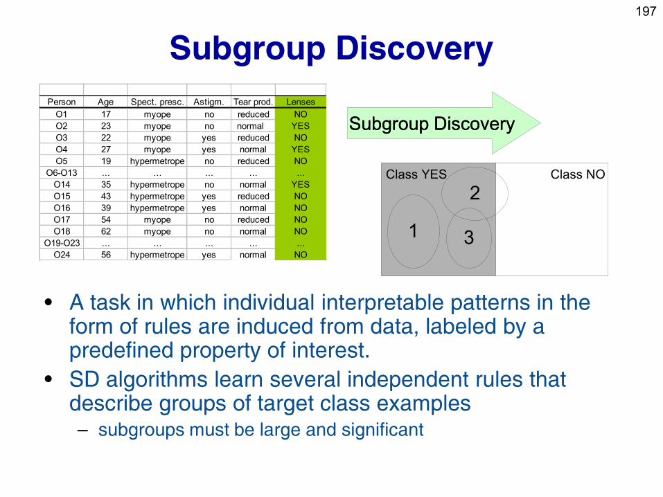
197
Subgroup Discovery
• A task in which individual interpretable patterns in the form of rules are induced from data, labeled by a predefined property of interest.
• SD algorithms learn several independent rules that describe groups of target class examples – subgroups must be large and significant
1
2
3
Class YES Class NO
Person Age Spect. presc. Astigm. Tear prod. Lenses
O1 17 myope no reduced NO
O2 23 myope no normal YES
O3 22 myope yes reduced NO
O4 27 myope yes normal YES
O5 19 hypermetrope no reduced NO
O6-O13 ... ... ... ... ...
O14 35 hypermetrope no normal YES
O15 43 hypermetrope yes reduced NO
O16 39 hypermetrope yes normal NO
O17 54 myope no reduced NO
O18 62 myope no normal NO
O19-O23 ... ... ... ... ...
O24 56 hypermetrope yes normal NO
Subgroup DiscoverySubgroup Discovery
198
Part IV. Descriptive DM techniques
• Predictive vs. descriptive induction
• Subgroup discovery
• Association rule learning
• Hierarchical clustering
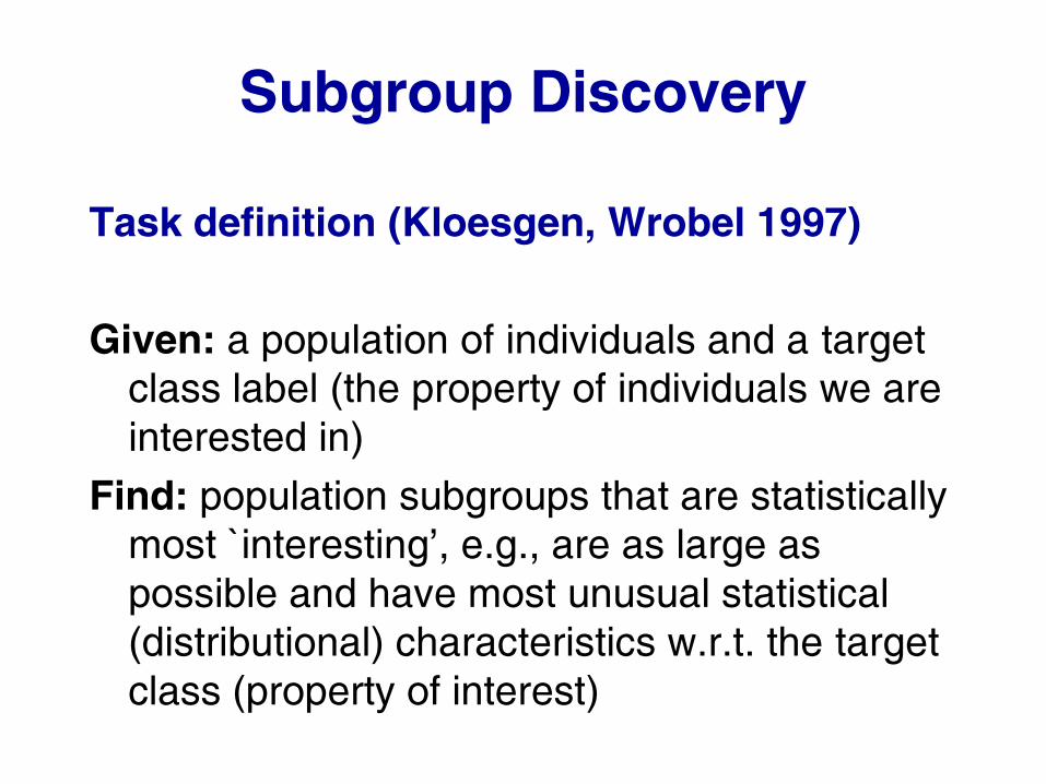
Subgroup Discovery
Task definition (Kloesgen, Wrobel 1997)
Given: a population of individuals and a target
class label (the property of individuals we are
interested in)
Find: population subgroups that are statistically
most `interesting’, e.g., are as large as
possible and have most unusual statistical
(distributional) characteristics w.r.t. the target
class (property of interest)
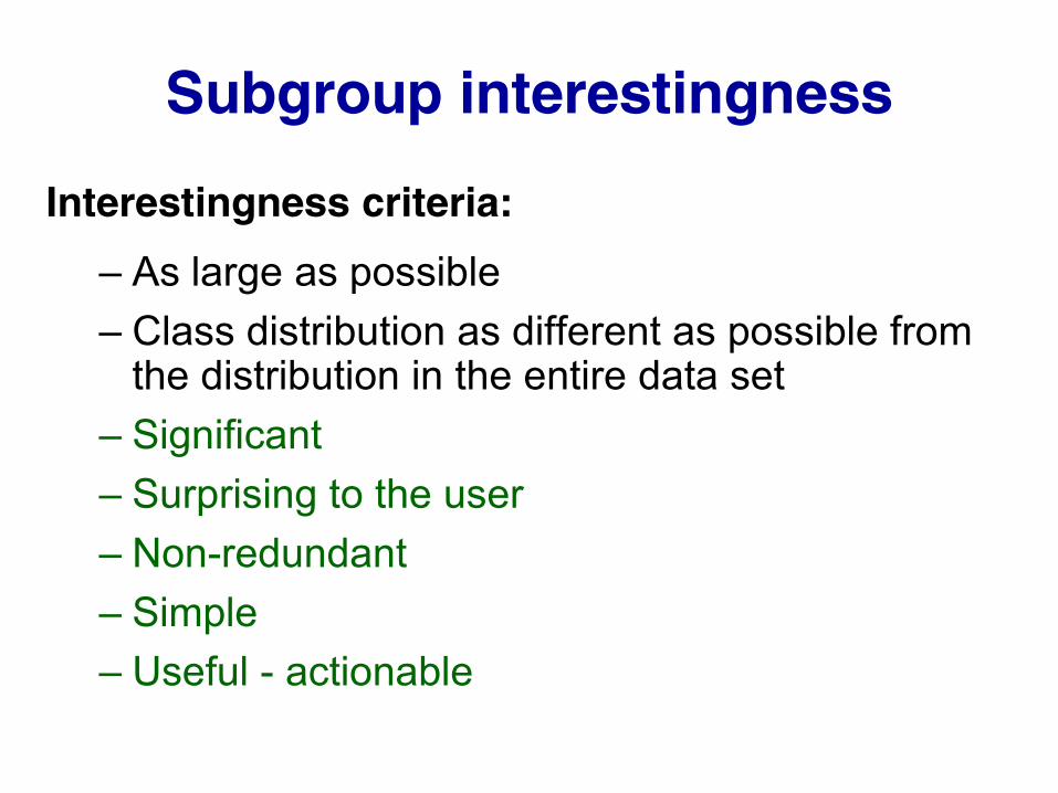
Subgroup interestingness
Interestingness criteria:
– As large as possible
– Class distribution as different as possible from the distribution in the entire data set
– Significant
– Surprising to the user
– Non-redundant
– Simple
– Useful - actionable
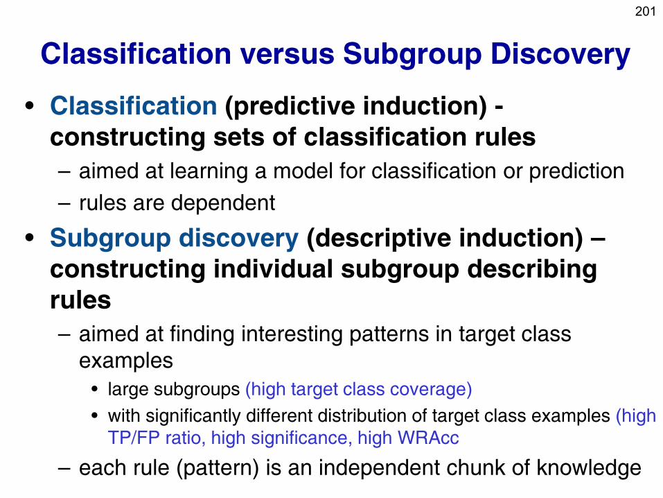
201
Classification versus Subgroup Discovery
• Classification (predictive induction) -
constructing sets of classification rules
– aimed at learning a model for classification or prediction
– rules are dependent
• Subgroup discovery (descriptive induction) –
constructing individual subgroup describing
rules
– aimed at finding interesting patterns in target class
examples
• large subgroups (high target class coverage)
• with significantly different distribution of target class examples (high
TP/FP ratio, high significance, high WRAcc
– each rule (pattern) is an independent chunk of knowledge
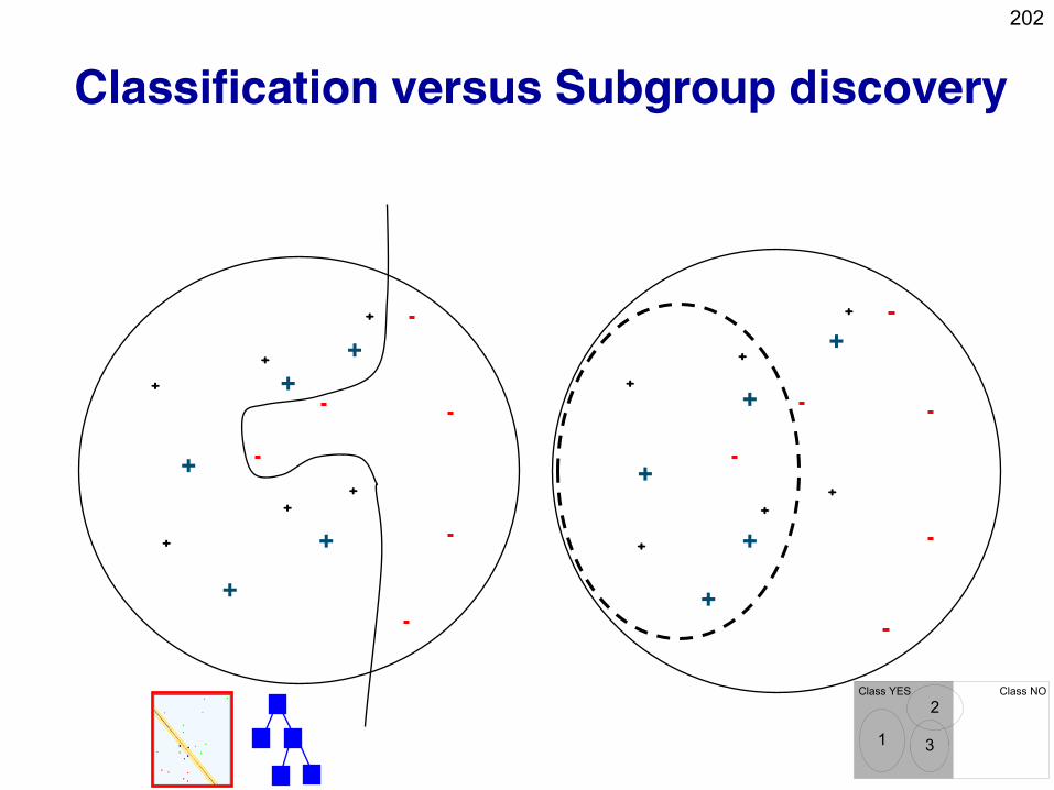
202
+
+
+
+
+
+
+
+
+
+
+
+
Classification versus Subgroup discovery
+
+
+
+
+ +
+
+
+
+
1
2
3
Class YES Class NO
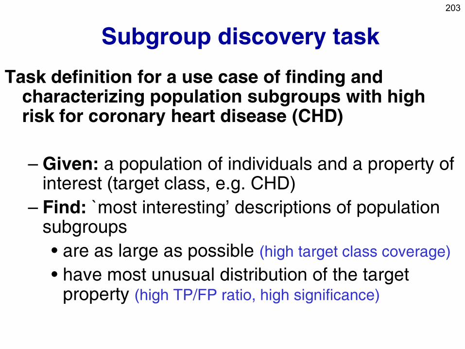
203
Subgroup discovery task
Task definition for a use case of finding and characterizing population subgroups with high risk for coronary heart disease (CHD)
– Given: a population of individuals and a property of interest (target class, e.g. CHD)
– Find: `most interesting’ descriptions of population subgroups
• are as large as possible (high target class coverage)
• have most unusual distribution of the target property (high TP/FP ratio, high significance)
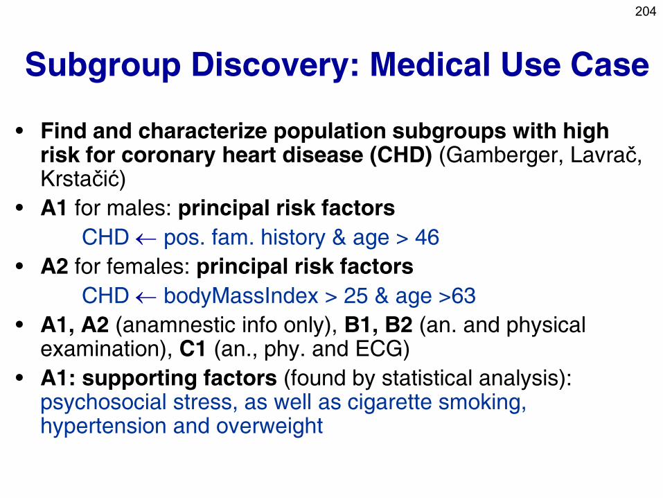
204
Subgroup Discovery: Medical Use Case
• Find and characterize population subgroups with high risk for coronary heart disease (CHD) (Gamberger, Lavrač, Krstačić)
• A1 for males: principal risk factors
CHD pos. fam. history & age > 46
• A2 for females: principal risk factors
CHD bodyMassIndex > 25 & age >63
• A1, A2 (anamnestic info only), B1, B2 (an. and physical examination), C1 (an., phy. and ECG)
• A1: supporting factors (found by statistical analysis): psychosocial stress, as well as cigarette smoking, hypertension and overweight
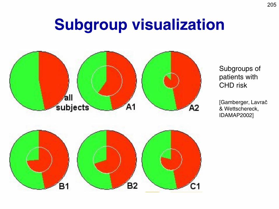
205
Subgroup visualization
Subgroups of
patients with
CHD risk
[Gamberger, Lavrač
& Wettschereck,
IDAMAP2002]
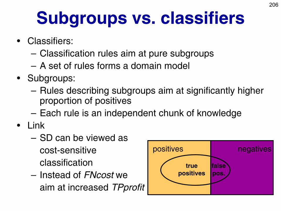
206
Subgroups vs. classifiers
• Classifiers:
– Classification rules aim at pure subgroups
– A set of rules forms a domain model
• Subgroups:
– Rules describing subgroups aim at significantly higher proportion of positives
– Each rule is an independent chunk of knowledge
• Link
– SD can be viewed as
cost-sensitive
classification
– Instead of FNcost we
aim at increased TPprofit
negatives positives
true
positives
false
pos.
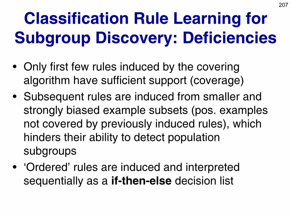
207
Classification Rule Learning for
Subgroup Discovery: Deficiencies
• Only first few rules induced by the covering
algorithm have sufficient support (coverage)
• Subsequent rules are induced from smaller and
strongly biased example subsets (pos. examples
not covered by previously induced rules), which
hinders their ability to detect population
subgroups
• ‘Ordered’ rules are induced and interpreted
sequentially as a if-then-else decision list
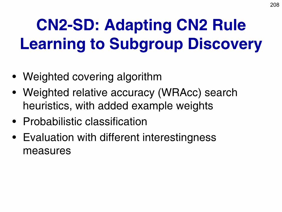
208
CN2-SD: Adapting CN2 Rule
Learning to Subgroup Discovery
• Weighted covering algorithm
• Weighted relative accuracy (WRAcc) search
heuristics, with added example weights
• Probabilistic classification
• Evaluation with different interestingness
measures
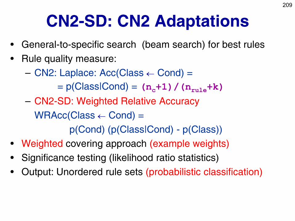
209
CN2-SD: CN2 Adaptations
• General-to-specific search (beam search) for best rules
• Rule quality measure:
– CN2: Laplace: Acc(Class Cond) =
= p(Class|Cond) = (nc+1)/(nrule+k)
– CN2-SD: Weighted Relative Accuracy
WRAcc(Class Cond) =
p(Cond) (p(Class|Cond) - p(Class))
• Weighted covering approach (example weights)
• Significance testing (likelihood ratio statistics)
• Output: Unordered rule sets (probabilistic classification)
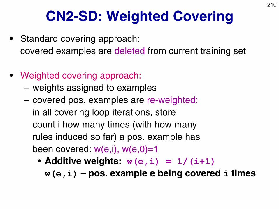
210
CN2-SD: Weighted Covering
• Standard covering approach:
covered examples are deleted from current training set
• Weighted covering approach:
– weights assigned to examples
– covered pos. examples are re-weighted:
in all covering loop iterations, store
count i how many times (with how many
rules induced so far) a pos. example has
been covered: w(e,i), w(e,0)=1
• Additive weights: w(e,i) = 1/(i+1)
w(e,i) – pos. example e being covered i times
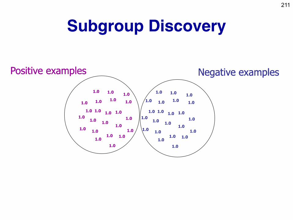
211
Subgroup Discovery
1.0 1.0
1.0
1.0
1.0
1.0
1.0
1.0
1.0
1.0 1.0 1.0
1.0
1.0
1.0
1.0
1.0 1.0
1.0
1.0
1.0 1.0
1.0
1.0 1.0
1.0
1.0
1.0
1.0
1.0
1.0
1.0
1.0 1.0
1.0
1.0
1.0
1.0
1.0 1.0
1.0
1.0
1.0 1.0
1.0
Positive examplesPositive examples NNegative examplesegative examples
1.0
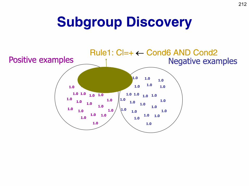
212
Subgroup Discovery
1.0 1.0
1.0
1.0
1.0
1.0
1.0
1.0
1.0
1.0 1.0 1.0
1.0
1.0
1.0
1.0
1.0 1.0
1.0
1.0
1.0 1.0
1.0
1.0 1.0
1.0
1.0
1.0
1.0
1.0
1.0
1.0
1.0 1.0 1.0
1.0
1.0
1.0
1.0
1.0 1.0
1.0
1.0
1.0 1.0
1.0
Positive examplesPositive examples NNegative examplesegative examples Rule1: Cl=+ Rule1: Cl=+ Cond6 AND Cond2Cond6 AND Cond2
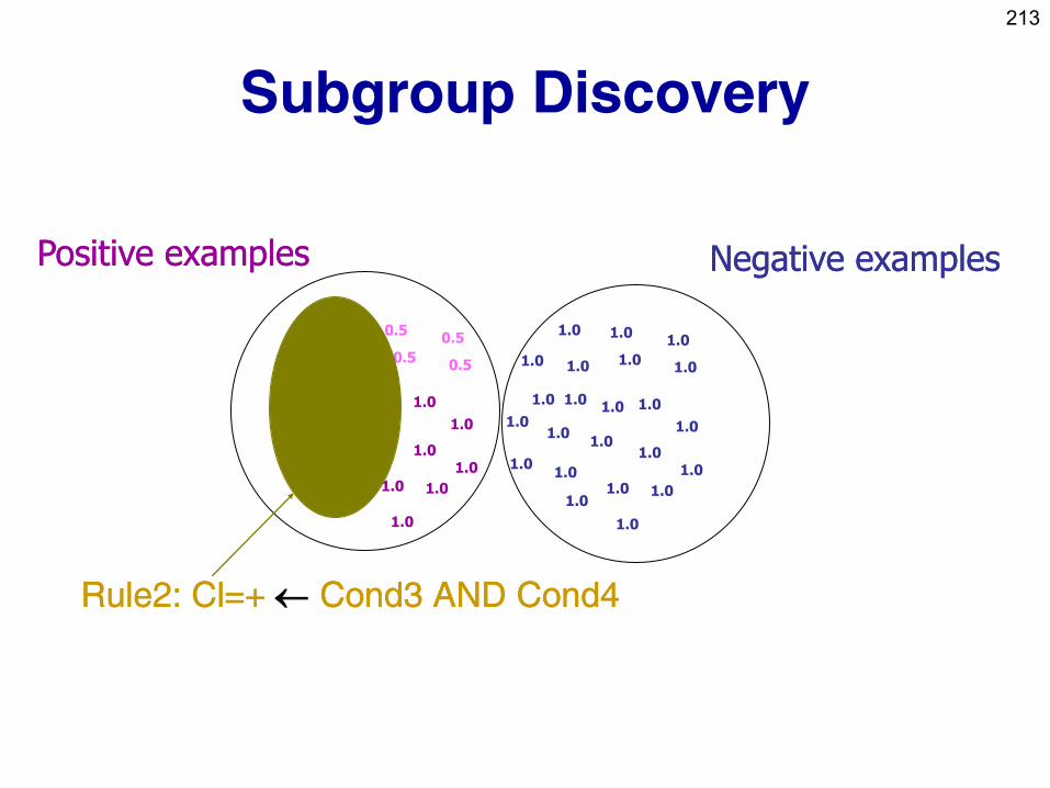
213
Subgroup Discovery
0.5 0.5
1.0
0.5
0.5
1.0
1.0
1.0
1.0
0.5 1.0 0.5
1.0
1.0
1.0
1.0
1.0 1.0
1.0
1.0
1.0 1.0
1.0
1.0 1.0
1.0
1.0
1.0
1.0
1.0
1.0
1.0
1.0 1.0 1.0
1.0
1.0
1.0
1.0
1.0 1.0
1.0
1.0
1.0 1.0
1.0
Positive examplesPositive examples NNegative examplesegative examples
Rule2: Cl=+ Rule2: Cl=+ Cond3 AND Cond4Cond3 AND Cond4
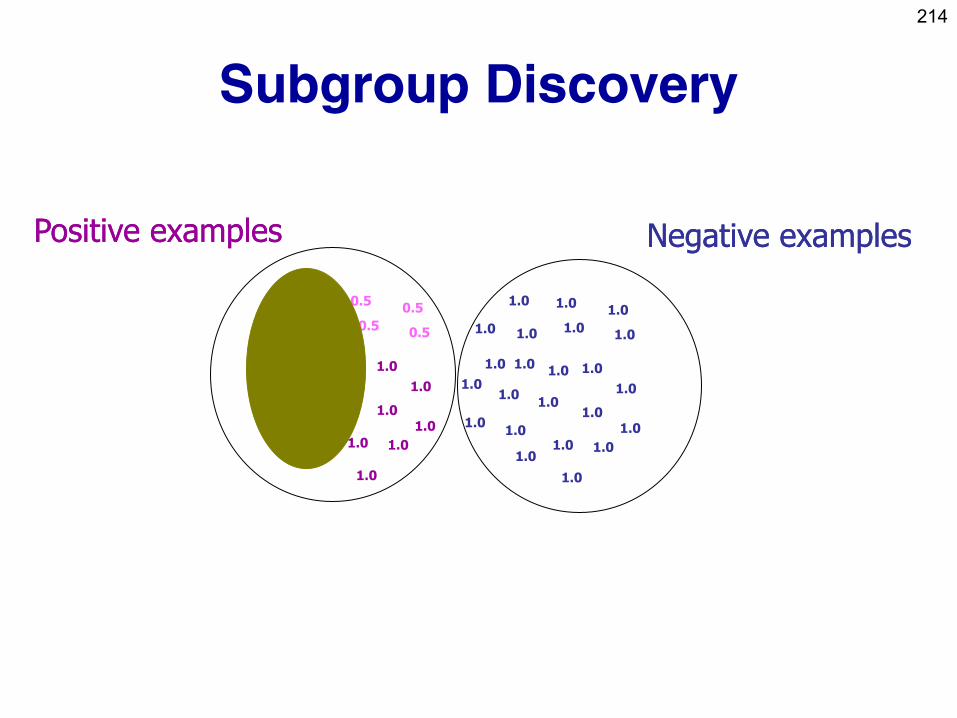
214
Subgroup Discovery
0.5 0.5
0.5
0.25
0.5
0.5
0.5
0.5
1.0
0.5 0..5 0.25
0.5
1.0
1.0
0.5
0.5 0.5
1.0
1.0
1.0 0.5
1.0
1.0 1.0
1.0
1.0
1.0
1.0
1.0
1.0
1.0
1.0 1.0 1.0
1.0
1.0
1.0
1.0
1.0 1.0
1.0
1.0
1.0 1.0
1.0
Positive examplesPositive examples NNegative examplesegative examples
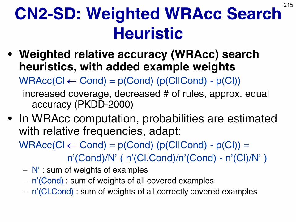
215
CN2-SD: Weighted WRAcc Search
Heuristic • Weighted relative accuracy (WRAcc) search
heuristics, with added example weights WRAcc(Cl Cond) = p(Cond) (p(Cl|Cond) - p(Cl))
increased coverage, decreased # of rules, approx. equal accuracy (PKDD-2000)
• In WRAcc computation, probabilities are estimated with relative frequencies, adapt:
WRAcc(Cl Cond) = p(Cond) (p(Cl|Cond) - p(Cl)) =
n’(Cond)/N’ ( n’(Cl.Cond)/n’(Cond) - n’(Cl)/N’ ) – N’ : sum of weights of examples
– n’(Cond) : sum of weights of all covered examples
– n’(Cl.Cond) : sum of weights of all correctly covered examples

216
Subgroup visualization
The CHD task: Find,
characterize and visualize
population subgroups with high
CHD risk (large enough,
distributionally unusual, most
actionable)
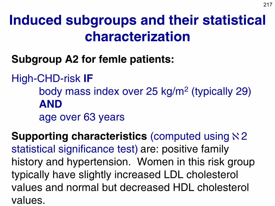
217
Induced subgroups and their statistical
characterization
Subgroup A2 for femle patients:
High-CHD-risk IF
body mass index over 25 kg/m2 (typically 29)
AND
age over 63 years
Supporting characteristics (computed using 2
statistical significance test) are: positive family
history and hypertension. Women in this risk group
typically have slightly increased LDL cholesterol
values and normal but decreased HDL cholesterol
values.
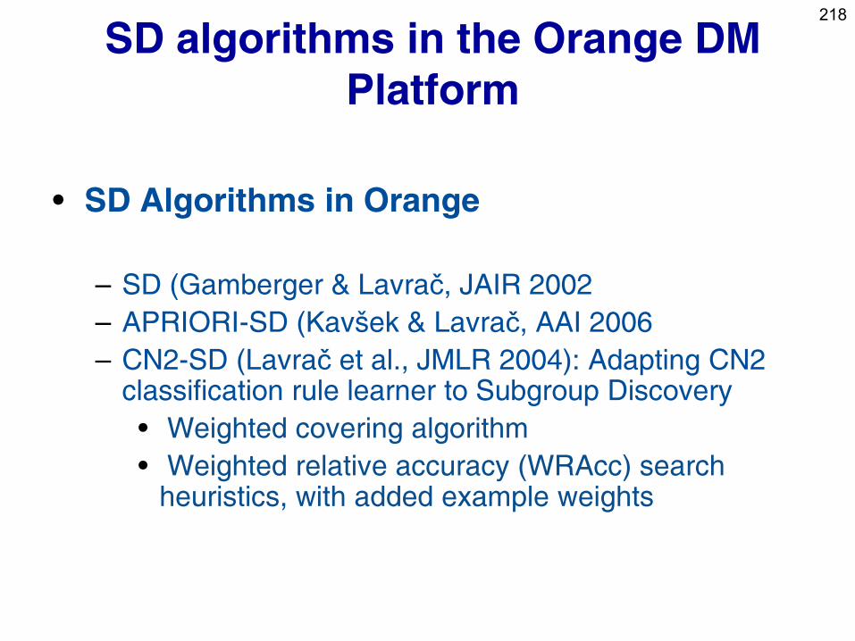
218
SD algorithms in the Orange DM
Platform
• SD Algorithms in Orange
– SD (Gamberger & Lavrač, JAIR 2002
– APRIORI-SD (Kavšek & Lavrač, AAI 2006
– CN2-SD (Lavrač et al., JMLR 2004): Adapting CN2 classification rule learner to Subgroup Discovery
• Weighted covering algorithm
• Weighted relative accuracy (WRAcc) search heuristics, with added example weights
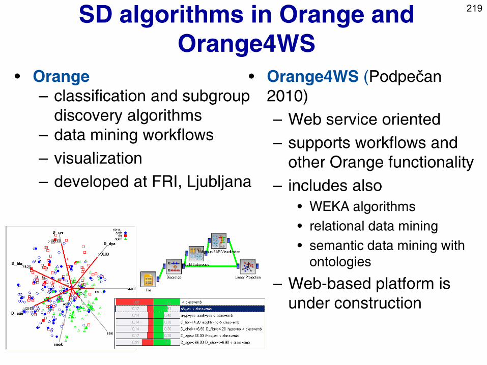
219 SD algorithms in Orange and
Orange4WS
• Orange
– classification and subgroup
discovery algorithms
– data mining workflows
– visualization
– developed at FRI, Ljubljana
• Orange4WS (Podpečan
2010)
– Web service oriented
– supports workflows and
other Orange functionality
– includes also
• WEKA algorithms
• relational data mining
• semantic data mining with
ontologies
– Web-based platform is
under construction
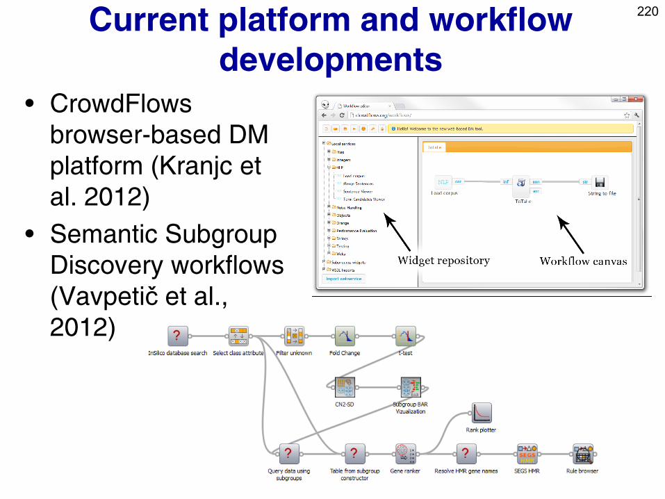
Current platform and workflow
developments
• CrowdFlows
browser-based DM
platform (Kranjc et
al. 2012)
• Semantic Subgroup
Discovery workflows
(Vavpetič et al.,
2012)
220
221
Part IV. Descriptive DM techniques
• Predictive vs. descriptive induction
• Subgroup discovery
• Association rule learning
• Hierarchical clustering
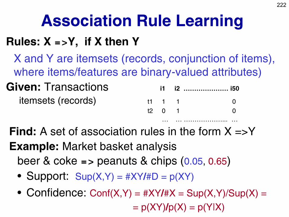
222
Association Rule Learning
Rules: X =>Y, if X then Y
X and Y are itemsets (records, conjunction of items),
where items/features are binary-valued attributes)
Given: Transactions i1 i2 ………………… i50
itemsets (records) t1 1 1 0
t2 0 1 0
… … ………………... …
Find: A set of association rules in the form X =>Y
Example: Market basket analysis
beer & coke => peanuts & chips (0.05, 0.65)
• Support: Sup(X,Y) = #XY/#D = p(XY)
• Confidence: Conf(X,Y) = #XY/#X = Sup(X,Y)/Sup(X) = = p(XY)/p(X) = p(Y|X)
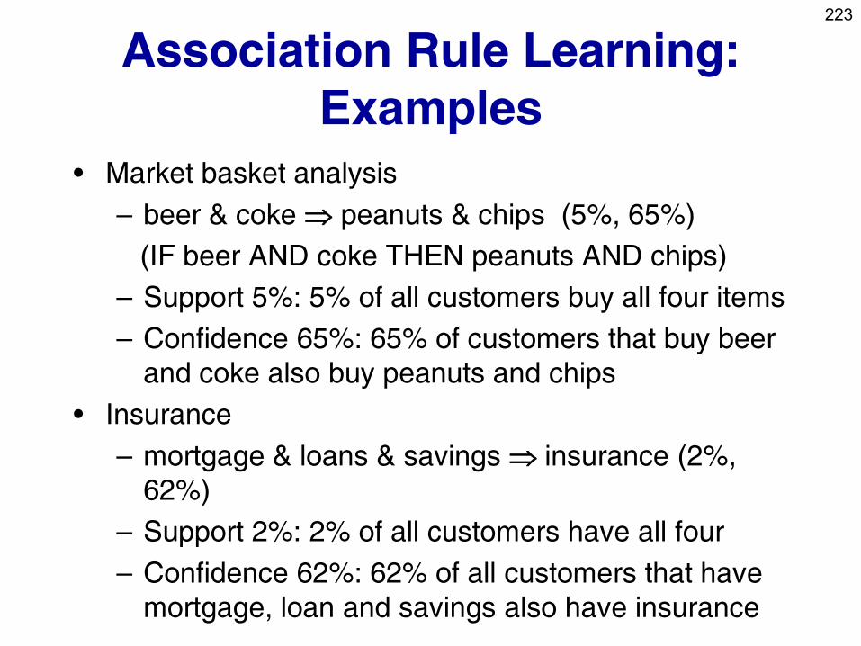
223
Association Rule Learning:
Examples
• Market basket analysis
– beer & coke peanuts & chips (5%, 65%)
(IF beer AND coke THEN peanuts AND chips)
– Support 5%: 5% of all customers buy all four items
– Confidence 65%: 65% of customers that buy beer
and coke also buy peanuts and chips
• Insurance
– mortgage & loans & savings insurance (2%,
62%)
– Support 2%: 2% of all customers have all four
– Confidence 62%: 62% of all customers that have
mortgage, loan and savings also have insurance
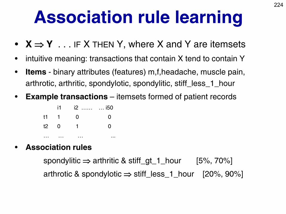
224
Association rule learning
• X Y . . . IF X THEN Y, where X and Y are itemsets
• intuitive meaning: transactions that contain X tend to contain Y
• Items - binary attributes (features) m,f,headache, muscle pain,
arthrotic, arthritic, spondylotic, spondylitic, stiff_less_1_hour
• Example transactions – itemsets formed of patient records
i1 i2 …… … i50
t1 1 0 0
t2 0 1 0
… … … ...
• Association rules
spondylitic arthritic & stiff_gt_1_hour [5%, 70%]
arthrotic & spondylotic stiff_less_1_hour [20%, 90%]
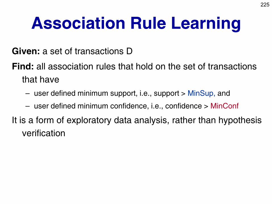
225
Association Rule Learning
Given: a set of transactions D
Find: all association rules that hold on the set of transactions
that have
– user defined minimum support, i.e., support > MinSup, and
– user defined minimum confidence, i.e., confidence > MinConf
It is a form of exploratory data analysis, rather than hypothesis
verification
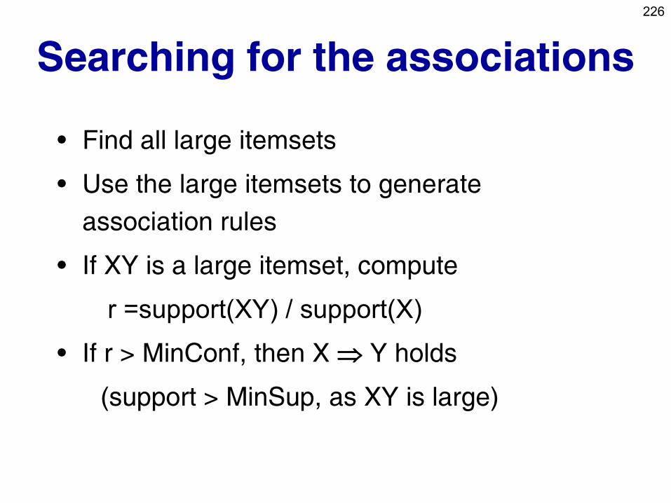
226
Searching for the associations
• Find all large itemsets
• Use the large itemsets to generate
association rules
• If XY is a large itemset, compute
r =support(XY) / support(X)
• If r > MinConf, then X Y holds
(support > MinSup, as XY is large)
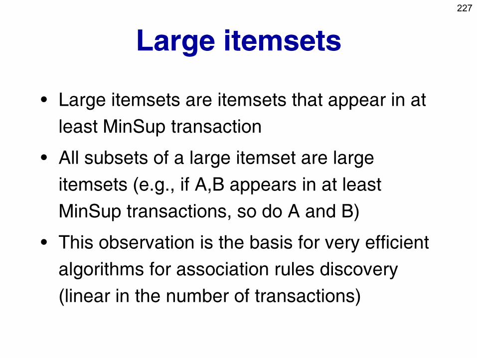
227
Large itemsets
• Large itemsets are itemsets that appear in at
least MinSup transaction
• All subsets of a large itemset are large
itemsets (e.g., if A,B appears in at least
MinSup transactions, so do A and B)
• This observation is the basis for very efficient
algorithms for association rules discovery
(linear in the number of transactions)
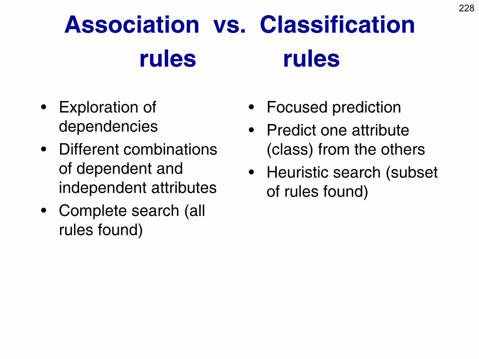
228
Association vs. Classification
rules rules
• Exploration of
dependencies
• Different combinations
of dependent and
independent attributes
• Complete search (all
rules found)
• Focused prediction
• Predict one attribute
(class) from the others
• Heuristic search (subset
of rules found)
229
Part IV. Descriptive DM techniques
• Predictive vs. descriptive induction
• Subgroup discovery
• Association rule learning
• Hierarchical clustering
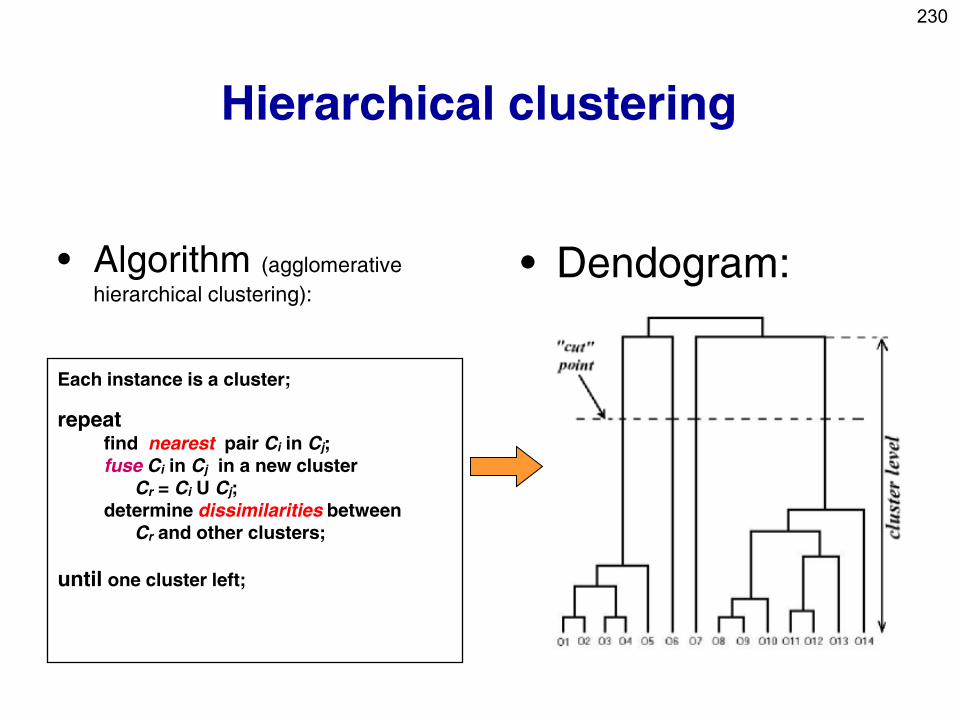
230
Hierarchical clustering
• Algorithm (agglomerative
hierarchical clustering):
Each instance is a cluster;
repeat find nearest pair Ci in Cj;
fuse Ci in Cj in a new cluster
Cr = Ci U Cj;
determine dissimilarities between
Cr and other clusters;
until one cluster left;
• Dendogram:
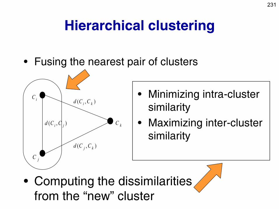
231
Hierarchical clustering
• Fusing the nearest pair of clusters
iC
jC
kC),( ji CCd
),( ki CCd
),( kj CCd
• Minimizing intra-cluster
similarity
• Maximizing inter-cluster
similarity
• Computing the dissimilarities
from the “new” cluster
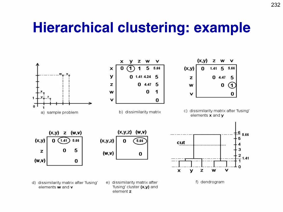
232
Hierarchical clustering: example
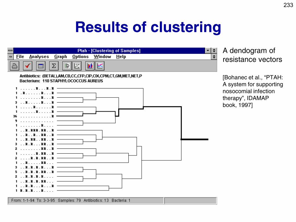
233
Results of clustering
A dendogram of
resistance vectors
[Bohanec et al., “PTAH:
A system for supporting
nosocomial infection
therapy”, IDAMAP
book, 1997]
234
Part V:
Relational Data Mining
• What is RDM
• Propositionalization techniques
• Semantic Data Mining
• Inductive Logic programming
• Learning as search in Inductive Logic
Programming
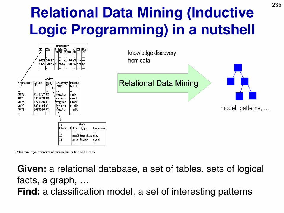
235
Relational Data Mining (Inductive
Logic Programming) in a nutshell
Relational Relational Data MiningData Mining
knowledge discovery
from data
model, patterns, …
Given: a relational database, a set of tables. sets of logical
facts, a graph, …
Find: a classification model, a set of interesting patterns
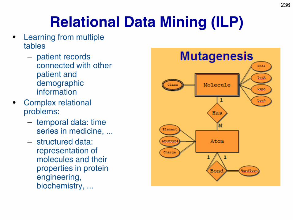
236
Relational Data Mining (ILP) • Learning from multiple
tables
– patient records connected with other patient and demographic information
• Complex relational problems:
– temporal data: time series in medicine, ...
– structured data: representation of molecules and their properties in protein engineering, biochemistry, ...
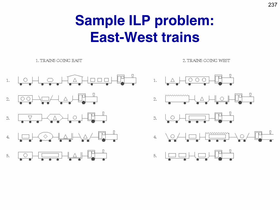
237
Sample ILP problem:
East-West trains
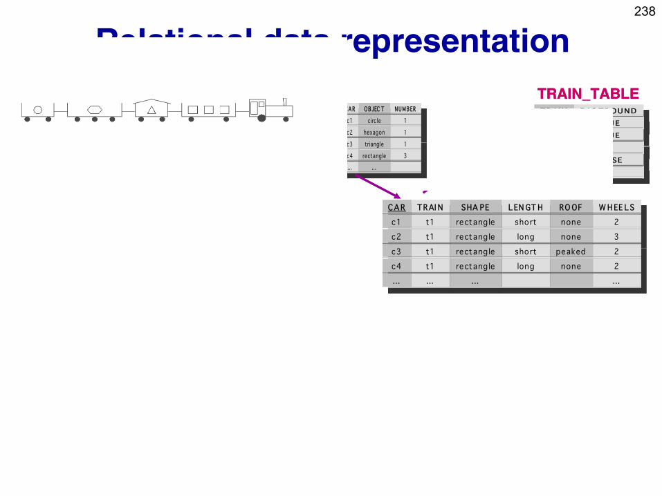
238
Relational data representation
TRAI N EAS TB OU ND
t1 TRU E
t2 TRU E
… …
t6 FAL SE
… …
TRAIN_TABLE TRAIN_TABLE
CA R TRAI N SHA PE LEN GT H RO OF W H EE LS
c1 t1 rectang le short none 2
c2 t1 rectang le long none 3
c3 t1 rectang le short peaked 2
c4 t1 rectang le long none 2
… … … …
LO AD CA R O B JEC T NU M B ER
l1 c1 circ le 1
l2 c2 hexagon 1
l3 c3 triangl e 1
l4 c4 rectang le 3
… … …
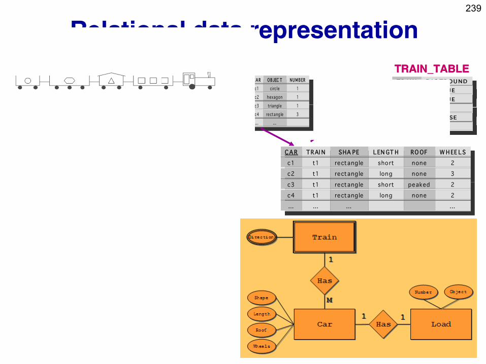
239
Relational data representation
TRAI N EAS TB OU ND
t1 TRU E
t2 TRU E
… …
t6 FAL SE
… …
TRAIN_TABLE TRAIN_TABLE
CA R TRAI N SHA PE LEN GT H RO OF W H EE LS
c1 t1 rectang le short none 2
c2 t1 rectang le long none 3
c3 t1 rectang le short peaked 2
c4 t1 rectang le long none 2
… … … …
LO AD CA R O B JEC T NU M B ER
l1 c1 circ le 1
l2 c2 hexagon 1
l3 c3 triangl e 1
l4 c4 rectang le 3
… … …
240
Part V:
Relational Data Mining
• What is RDM
• Propositionalization techniques
• Semantic Data Mining
• Inductive Logic programming
• Learning as search in Inductive Logic
Programming
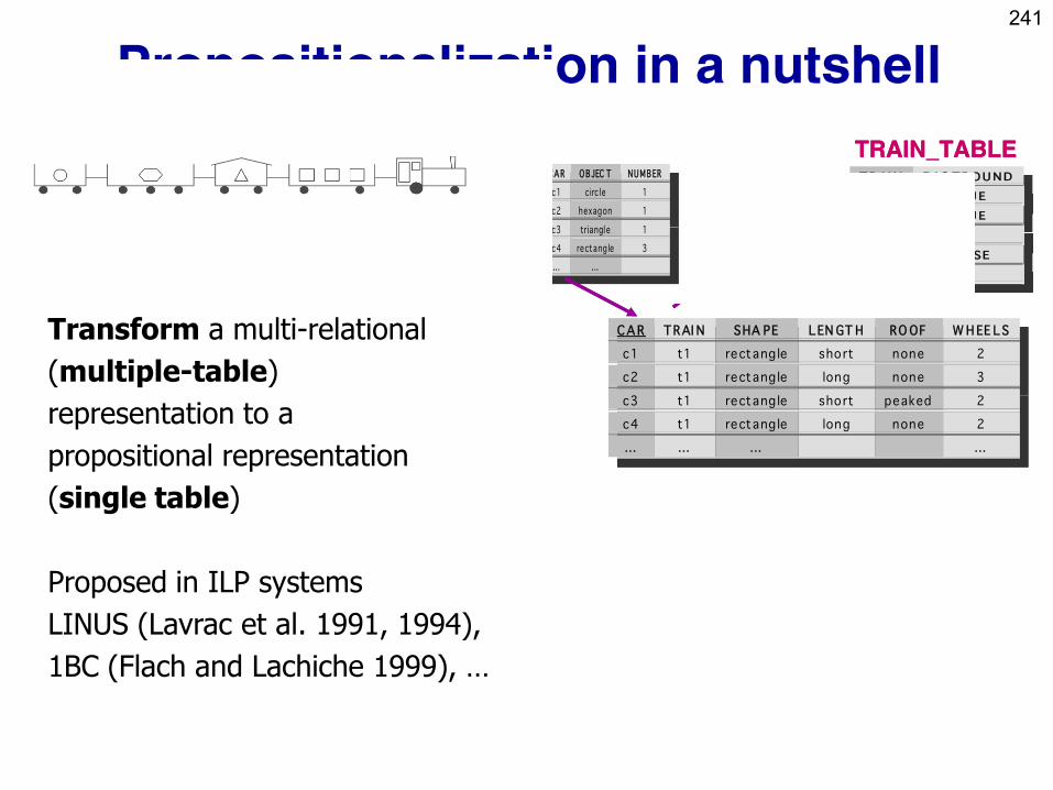
241
Propositionalization in a nutshell
TRAI N EAS TB OU ND
t1 TRU E
t2 TRU E
… …
t6 FAL SE
… …
TRAIN_TABLE TRAIN_TABLE
CA R TRAI N SHA PE LEN GT H RO OF W H EE LS
c1 t1 rectang le short none 2
c2 t1 rectang le long none 3
c3 t1 rectang le short peaked 2
c4 t1 rectang le long none 2
… … … …
LO AD CA R O B JEC T NU M B ER
l1 c1 circ le 1
l2 c2 hexagon 1
l3 c3 triangl e 1
l4 c4 rectang le 3
… … …
Propositionalization task
Transform a multi-relational
(multiple-table)
representation to a
propositional representation
(single table)
Proposed in ILP systems
LINUS (Lavrac et al. 1991, 1994),
1BC (Flach and Lachiche 1999), …
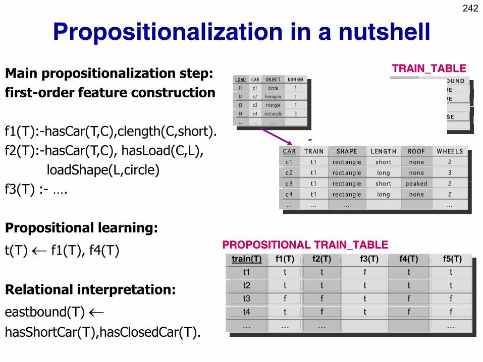
242
Propositionalization in a nutshell
TRAI N EAS TB OU ND
t1 TRU E
t2 TRU E
… …
t6 FAL SE
… …
TRAIN_TABLE TRAIN_TABLE
CA R TRAI N SHA PE LEN GT H RO OF W H EE LS
c1 t1 rectang le short none 2
c2 t1 rectang le long none 3
c3 t1 rectang le short peaked 2
c4 t1 rectang le long none 2
… … … …
LO AD CA R O B JEC T NU M B ER
l1 c1 circ le 1
l2 c2 hexagon 1
l3 c3 triangl e 1
l4 c4 rectang le 3
… … …
train(T) f1(T) f2(T) f3(T) f4(T) f5(T)
t1 t t f t t
t2 t t t t t
t3 f f t f f
t4 t f t f f
… … … …
PROPOSITIONAL TRAIN_TABLE PROPOSITIONAL TRAIN_TABLE
Main propositionalization step:
first-order feature construction
f1(T):-hasCar(T,C),clength(C,short).
f2(T):-hasCar(T,C), hasLoad(C,L),
loadShape(L,circle)
f3(T) :- ….
Propositional learning:
t(T) f1(T), f4(T)
Relational interpretation:
eastbound(T)
hasShortCar(T),hasClosedCar(T).
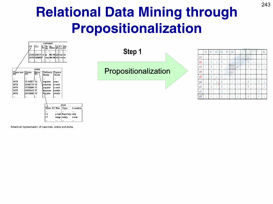
243
Relational Data Mining through
Propositionalization
PropositionalizationPropositionalization
Step 1
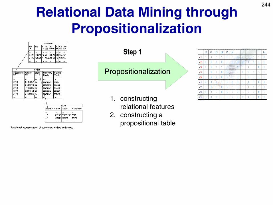
244
Relational Data Mining through
Propositionalization
PropositionalizationPropositionalization
Step 1
1. constructing
relational features
2. constructing a
propositional table
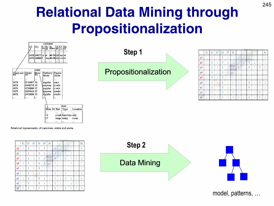
245
Relational Data Mining through
Propositionalization
PropositionalizationPropositionalization
model, patterns, …
Data MiningData Mining
Step 1
Step 2
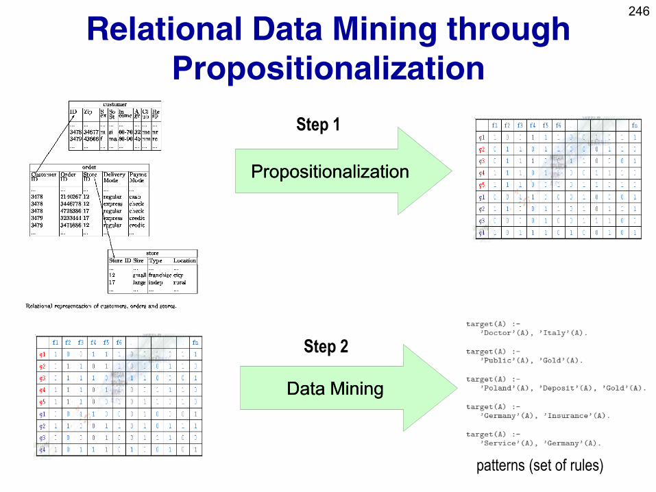
246
Relational Data Mining through
Propositionalization
PropositionalizationPropositionalization
patterns (set of rules)
Data MiningData Mining
Step 1
Step 2
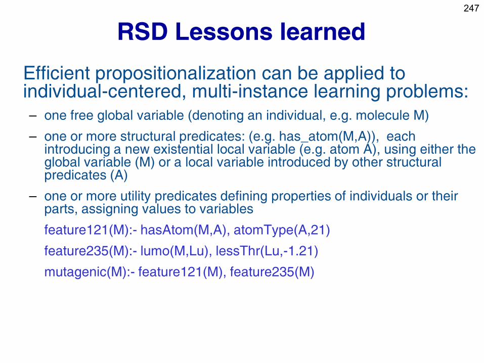
247
RSD Lessons learned
Efficient propositionalization can be applied to individual-centered, multi-instance learning problems:
– one free global variable (denoting an individual, e.g. molecule M)
– one or more structural predicates: (e.g. has_atom(M,A)), each introducing a new existential local variable (e.g. atom A), using either the global variable (M) or a local variable introduced by other structural predicates (A)
– one or more utility predicates defining properties of individuals or their parts, assigning values to variables
feature121(M):- hasAtom(M,A), atomType(A,21)
feature235(M):- lumo(M,Lu), lessThr(Lu,-1.21)
mutagenic(M):- feature121(M), feature235(M)
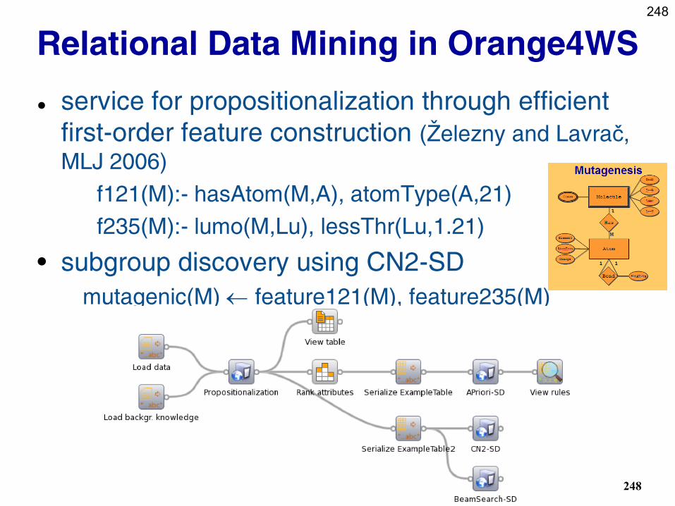
248
248
Relational Data Mining in Orange4WS
service for propositionalization through efficient
first-order feature construction (Železny and Lavrač,
MLJ 2006)
f121(M):- hasAtom(M,A), atomType(A,21)
f235(M):- lumo(M,Lu), lessThr(Lu,1.21)
• subgroup discovery using CN2-SD
mutagenic(M) feature121(M), feature235(M)
249
Part V:
Relational Data Mining
• What is RDM
• Propositionalization techniques
• Semantic Data Mining
• Inductive Logic programming
• Learning as search in Inductive Logic
Programming
What is Semantic Data Mining
• Ontology-driven (semantic) data mining is an
emerging research topic
• Semantic Data Mining (SDM) - a new term
denoting:
– the new challenge of mining semantically annotated
resources, with ontologies used as background
knowledge to data mining
– approaches with which semantic data are mined
250
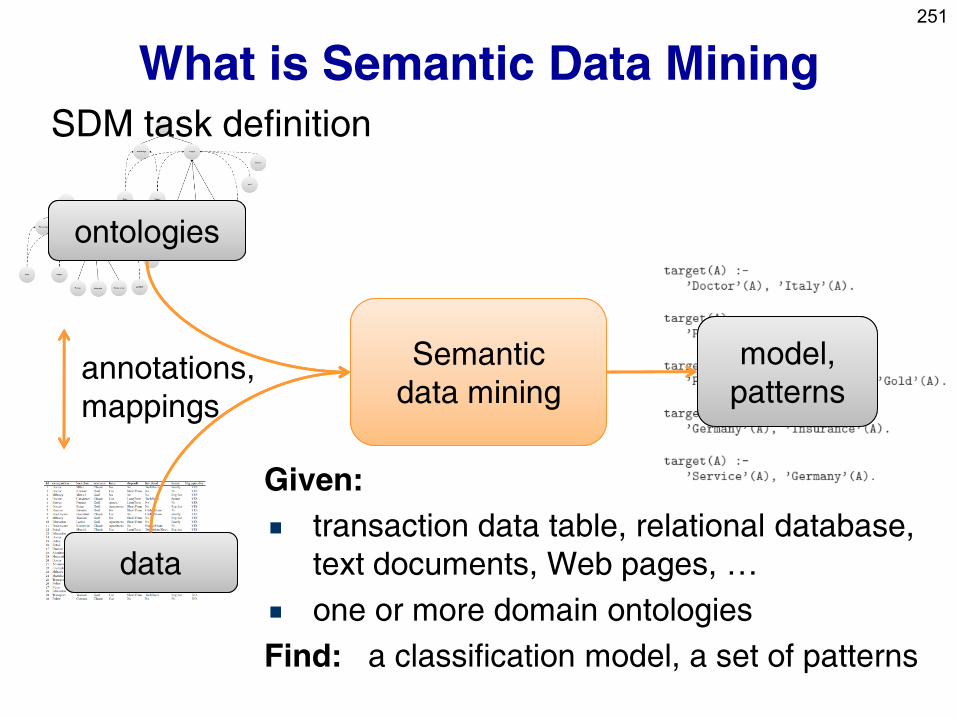
What is Semantic Data Mining
Semantic
data mining annotations,
mappings
ontologies
data
model,
patterns
SDM task definition
Given:
transaction data table, relational database,
text documents, Web pages, …
one or more domain ontologies
Find: a classification model, a set of patterns
251
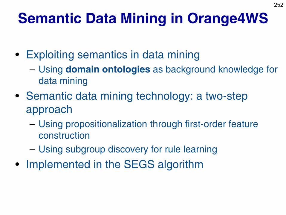
252
Semantic Data Mining in Orange4WS
• Exploiting semantics in data mining
– Using domain ontologies as background knowledge for
data mining
• Semantic data mining technology: a two-step
approach
– Using propositionalization through first-order feature
construction
– Using subgroup discovery for rule learning
• Implemented in the SEGS algorithm
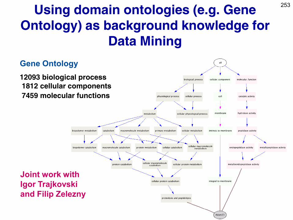
253
Using domain ontologies (e.g. Gene
Ontology) as background knowledge for
Data Mining
Gene Ontology
12093 biological process
1812 cellular components
7459 molecular functions
Joint work with
Igor Trajkovski
and Filip Zelezny
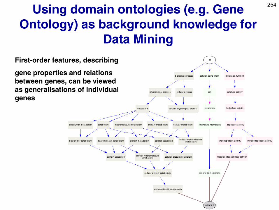
254
Using domain ontologies (e.g. Gene
Ontology) as background knowledge for
Data Mining
First-order features, describing
gene properties and relations
between genes, can be viewed
as generalisations of individual
genes
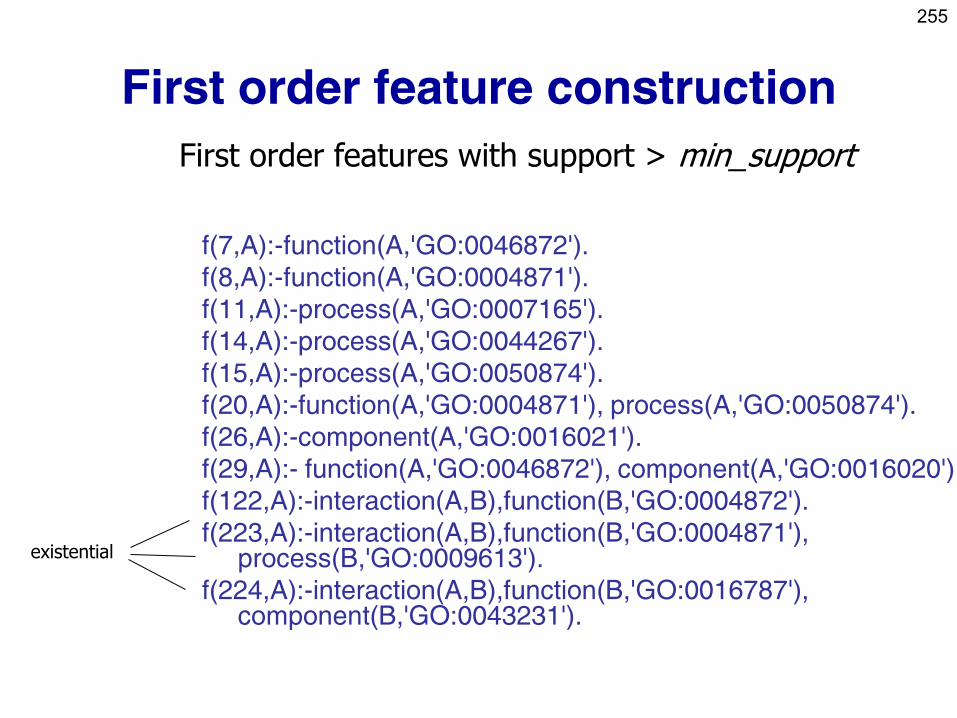
255
First order feature construction
f(7,A):-function(A,'GO:0046872').
f(8,A):-function(A,'GO:0004871').
f(11,A):-process(A,'GO:0007165').
f(14,A):-process(A,'GO:0044267').
f(15,A):-process(A,'GO:0050874').
f(20,A):-function(A,'GO:0004871'), process(A,'GO:0050874').
f(26,A):-component(A,'GO:0016021').
f(29,A):- function(A,'GO:0046872'), component(A,'GO:0016020').
f(122,A):-interaction(A,B),function(B,'GO:0004872').
f(223,A):-interaction(A,B),function(B,'GO:0004871'), process(B,'GO:0009613').
f(224,A):-interaction(A,B),function(B,'GO:0016787'), component(B,'GO:0043231').
First order features with support > min_support
existential
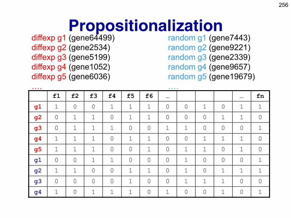
256
Propositionalization
f1 f2 f3 f4 f5 f6 … … fn
g1 1 0 0 1 1 1 0 0 1 0 1 1
g2 0 1 1 0 1 1 0 0 0 1 1 0
g3 0 1 1 1 0 0 1 1 0 0 0 1
g4 1 1 1 0 1 1 0 0 1 1 1 0
g5 1 1 1 0 0 1 0 1 1 0 1 0
g1 0 0 1 1 0 0 0 1 0 0 0 1
g2 1 1 0 0 1 1 0 1 0 1 1 1
g3 0 0 0 0 1 0 0 1 1 1 0 0
g4 1 0 1 1 1 0 1 0 0 1 0 1
diffexp g1 (gene64499)
diffexp g2 (gene2534)
diffexp g3 (gene5199)
diffexp g4 (gene1052)
diffexp g5 (gene6036)
….
random g1 (gene7443)
random g2 (gene9221)
random g3 (gene2339)
random g4 (gene9657)
random g5 (gene19679)
….
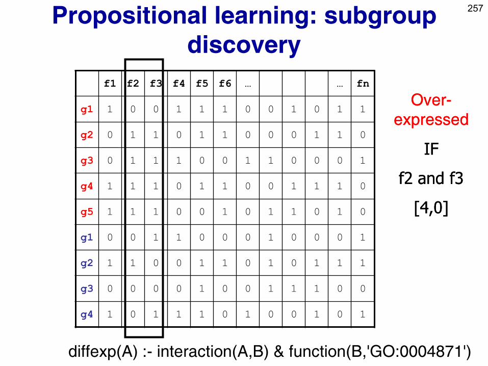
257
Propositional learning: subgroup
discovery
f1 f2 f3 f4 f5 f6 … … fn
g1 1 0 0 1 1 1 0 0 1 0 1 1
g2 0 1 1 0 1 1 0 0 0 1 1 0
g3 0 1 1 1 0 0 1 1 0 0 0 1
g4 1 1 1 0 1 1 0 0 1 1 1 0
g5 1 1 1 0 0 1 0 1 1 0 1 0
g1 0 0 1 1 0 0 0 1 0 0 0 1
g2 1 1 0 0 1 1 0 1 0 1 1 1
g3 0 0 0 0 1 0 0 1 1 1 0 0
g4 1 0 1 1 1 0 1 0 0 1 0 1
OverOver--
expressedexpressed
IF IF
f2 and f3f2 and f3
[4,0][4,0]
diffexp(A) :- interaction(A,B) & function(B,'GO:0004871')
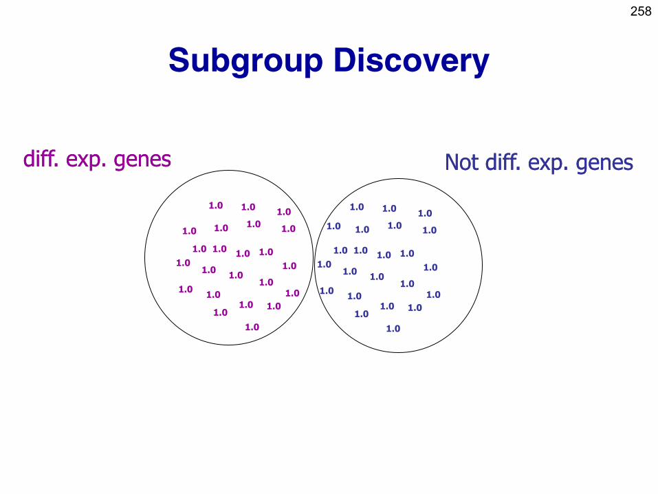
258
Subgroup Discovery
1.0 1.0
1.0
1.0
1.0
1.0
1.0
1.0
1.0
1.0 1.0 1.0
1.0
1.0
1.0
1.0
1.0 1.0
1.0
1.0
1.0 1.0
1.0
1.0 1.0
1.0
1.0
1.0
1.0
1.0
1.0
1.0
1.0 1.0
1.0
1.0
1.0
1.0
1.0 1.0
1.0
1.0
1.0 1.0
1.0
diff. exp. genesdiff. exp. genes Not diff. exp. genesNot diff. exp. genes
1.0
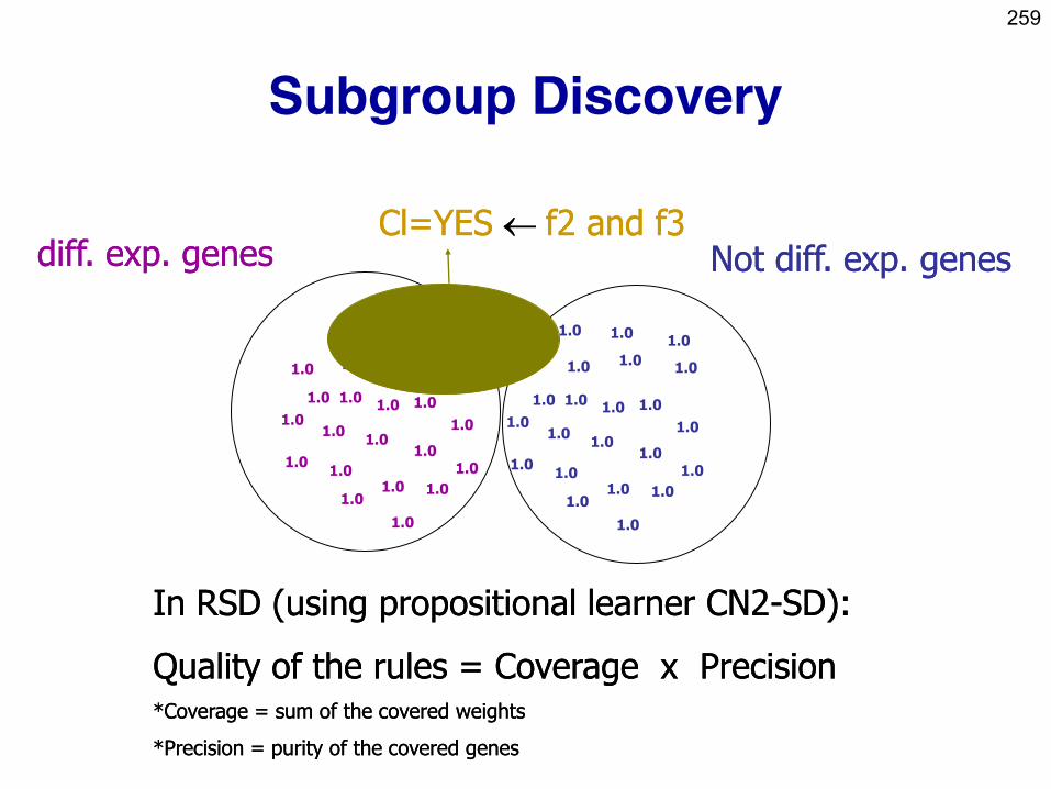
259
Subgroup Discovery
1.0 1.0
1.0
1.0
1.0
1.0
1.0
1.0
1.0
1.0 1.0 1.0
1.0
1.0
1.0
1.0
1.0 1.0
1.0
1.0
1.0 1.0
1.0
1.0 1.0
1.0
1.0
1.0
1.0
1.0
1.0
1.0
1.0 1.0 1.0
1.0
1.0
1.0
1.0
1.0 1.0
1.0
1.0
1.0 1.0
1.0
diff. exp. genesdiff. exp. genes Not diff. exp. genesNot diff. exp. genes Cl=Cl=YESYES f2 and f3f2 and f3
In RSD (using propositional learner CN2In RSD (using propositional learner CN2--SD):SD):
Quality of the rules = Coverage x PrecisionQuality of the rules = Coverage x Precision *Coverage = sum of the covered weights*Coverage = sum of the covered weights
*Precision = purity of the covered genes*Precision = purity of the covered genes
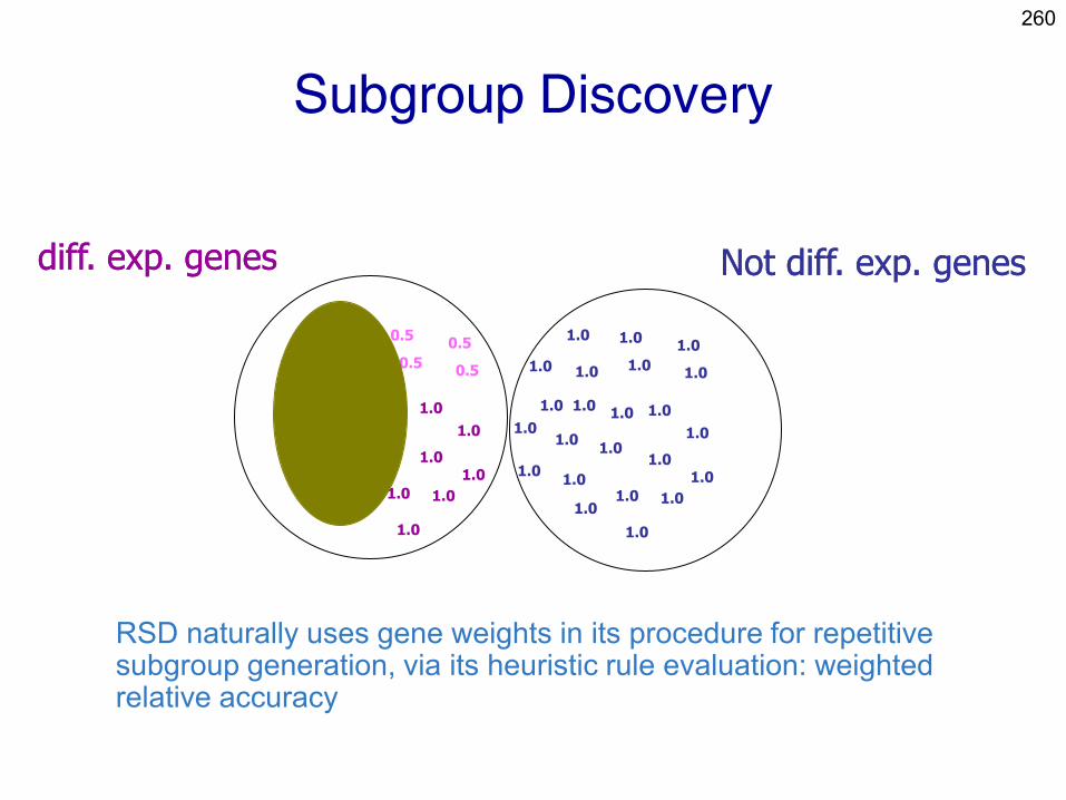
260
Subgroup Discovery
0.5 0.5
1.0
0.5
0.5
1.0
1.0
1.0
1.0
0.5 1.0 0.5
1.0
1.0
1.0
1.0
1.0 1.0
1.0
1.0
1.0 1.0
1.0
1.0 1.0
1.0
1.0
1.0
1.0
1.0
1.0
1.0
1.0 1.0 1.0
1.0
1.0
1.0
1.0
1.0 1.0
1.0
1.0
1.0 1.0
1.0
diff. exp. genesdiff. exp. genes Not diff. exp. genesNot diff. exp. genes
RSD naturally uses gene weights in its procedure for repetitive subgroup generation, via its heuristic rule evaluation: weighted relative accuracy
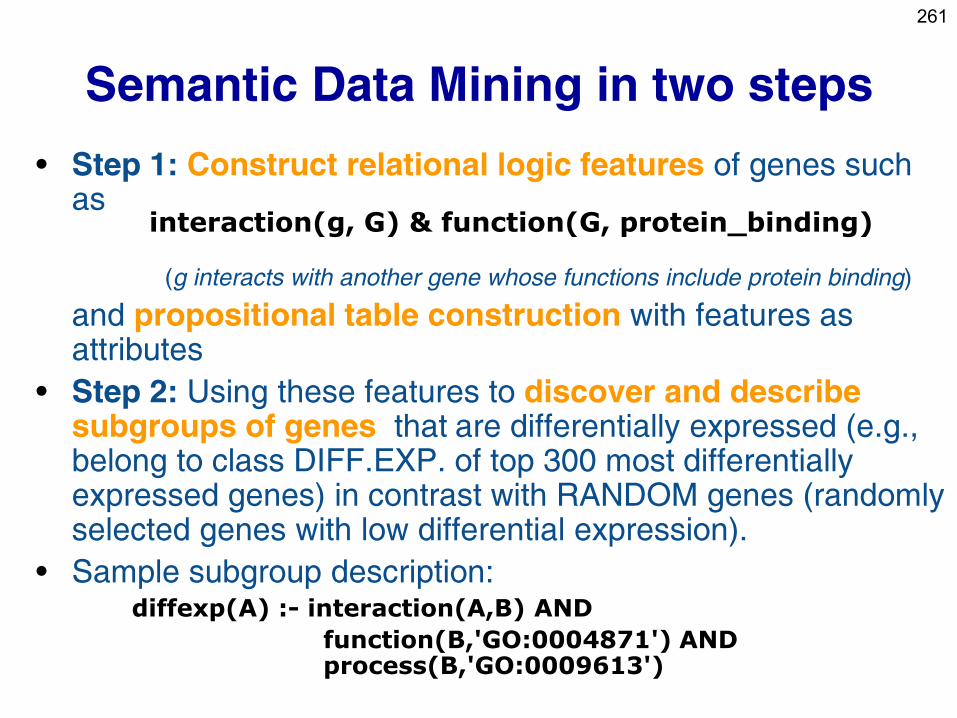
261
Semantic Data Mining in two steps
• Step 1: Construct relational logic features of genes such as
(g interacts with another gene whose functions include protein binding)
and propositional table construction with features as attributes
• Step 2: Using these features to discover and describe subgroups of genes that are differentially expressed (e.g., belong to class DIFF.EXP. of top 300 most differentially expressed genes) in contrast with RANDOM genes (randomly selected genes with low differential expression).
• Sample subgroup description: diffexp(A) :- interaction(A,B) AND
function(B,'GO:0004871') AND process(B,'GO:0009613')
interaction(g, G) & function(G, protein_binding)
262
Summary: SEGS, using the RSD
approach
• The SEGS approach enables to discover new
medical knowledge from the combination of gene
expression data with public gene annotation
databases
• The SEGS approach proved effective in several
biomedical applications (JBI 2008, …) • The work on semantic data mining - using ontologies as
background knowledge for subgroup discovery with SEGS - was
done in collaboration with I.Trajkovski, F. Železny and J. Tolar
• Recent work: Semantic subgroup discovery
implemented in Orange4WS
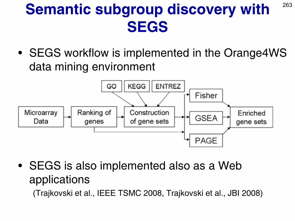
Semantic subgroup discovery with
SEGS
• SEGS workflow is implemented in the Orange4WS
data mining environment
• SEGS is also implemented also as a Web
applications (Trajkovski et al., IEEE TSMC 2008, Trajkovski et al., JBI 2008)
263
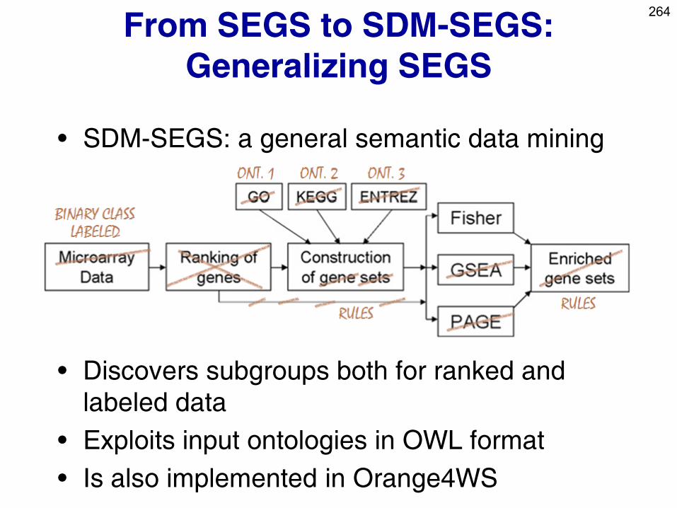
From SEGS to SDM-SEGS:
Generalizing SEGS
• SDM-SEGS: a general semantic data mining
system generalizing SEGS
• Discovers subgroups both for ranked and
labeled data
• Exploits input ontologies in OWL format
• Is also implemented in Orange4WS
264
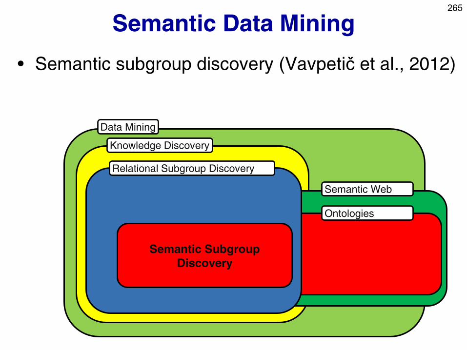
Semantic Data Mining
• Semantic subgroup discovery (Vavpetič et al., 2012)
Data Mining
Knowledge Discovery
Semantic Web
Ontologies
Relational Subgroup Discovery
Semantic Subgroup
Discovery
265
266
Part V:
Relational Data Mining
• What is RDM
• Propositionalization techniques
• Semantic Data Mining
• Inductive Logic programming
• Learning as search in Inductive Logic
Programming
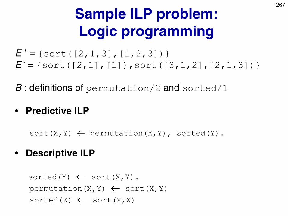
267
Sample ILP problem:
Logic programming
E + = {sort([2,1,3],[1,2,3])}
E - = {sort([2,1],[1]),sort([3,1,2],[2,1,3])}
B : definitions of permutation/2 and sorted/1
• Predictive ILP
sort(X,Y) permutation(X,Y), sorted(Y).
• Descriptive ILP
sorted(Y) sort(X,Y).
permutation(X,Y) sort(X,Y)
sorted(X) sort(X,X)
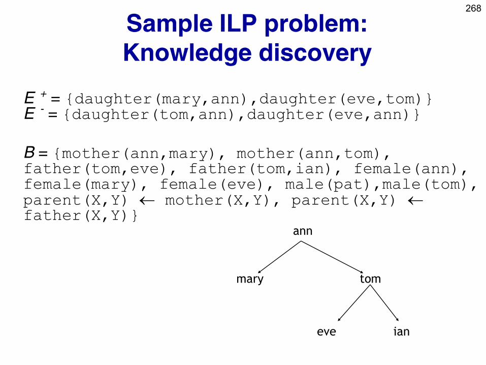
268
Sample ILP problem:
Knowledge discovery
E + = {daughter(mary,ann),daughter(eve,tom)} E - = {daughter(tom,ann),daughter(eve,ann)}
B = {mother(ann,mary), mother(ann,tom), father(tom,eve), father(tom,ian), female(ann), female(mary), female(eve), male(pat),male(tom), parent(X,Y) mother(X,Y), parent(X,Y) father(X,Y)}
ann
mary tom
eve ian
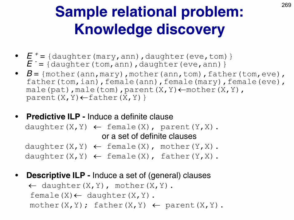
269
Sample relational problem:
Knowledge discovery
• E + = {daughter(mary,ann),daughter(eve,tom)} E - = {daughter(tom,ann),daughter(eve,ann)}
• B = {mother(ann,mary),mother(ann,tom),father(tom,eve), father(tom,ian),female(ann),female(mary),female(eve), male(pat),male(tom),parent(X,Y)mother(X,Y), parent(X,Y)father(X,Y)}
• Predictive ILP - Induce a definite clause
daughter(X,Y) female(X), parent(Y,X).
or a set of definite clauses
daughter(X,Y) female(X), mother(Y,X).
daughter(X,Y) female(X), father(Y,X).
• Descriptive ILP - Induce a set of (general) clauses
daughter(X,Y), mother(X,Y).
female(X) daughter(X,Y).
mother(X,Y); father(X,Y) parent(X,Y).
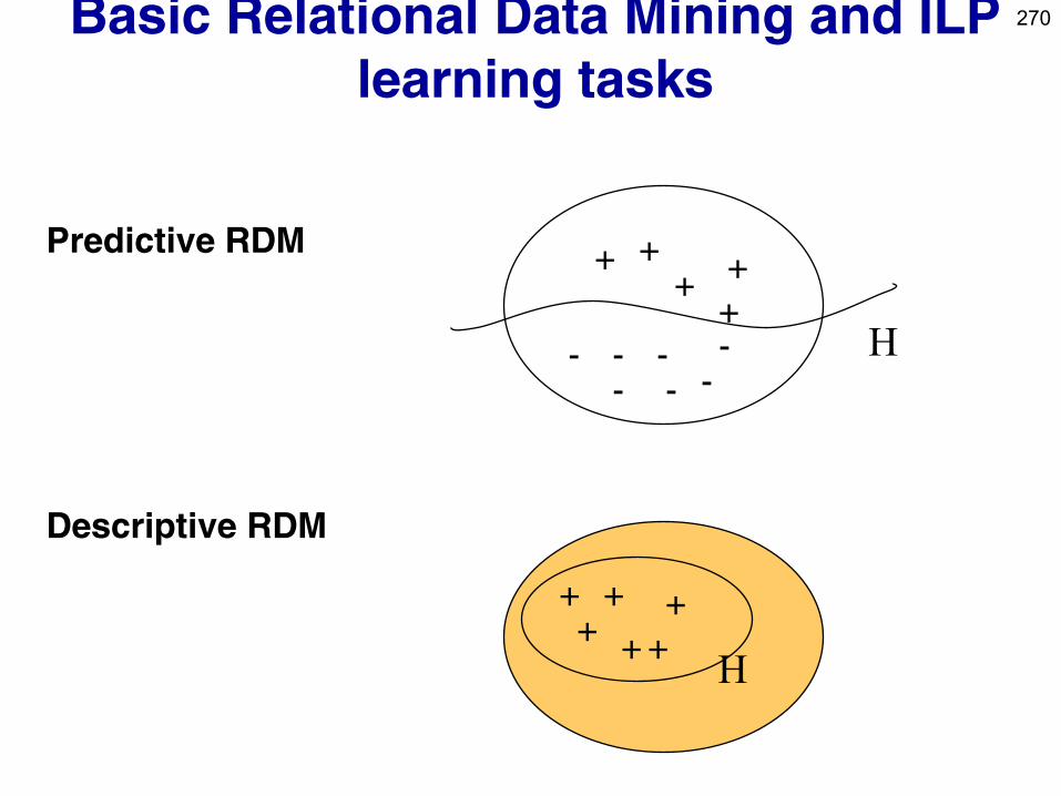
270 Basic Relational Data Mining and ILP
learning tasks
Predictive RDM
Descriptive RDM
+
-
+ +
+
+
- -
- - -
-
+ + +
+ + +
H
H
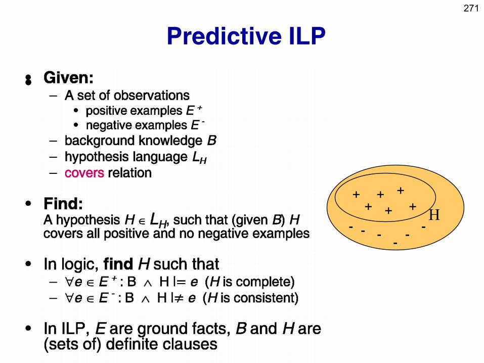
271
Predictive ILP
•
+ + + + + +
- - - - -
-
H
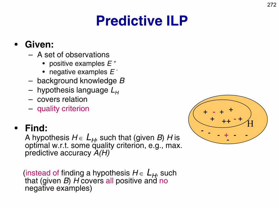
272
Predictive ILP
• Given: – A set of observations
• positive examples E +
• negative examples E -
– background knowledge B
– hypothesis language LH
– covers relation
– quality criterion
• Find: A hypothesis H LH, such that (given B) H is optimal w.r.t. some quality criterion, e.g., max. predictive accuracy A(H)
(instead of finding a hypothesis H LH, such that (given B) H covers all positive and no negative examples)
+ +
+ +
- - - - -
-
H
+
+ + +
- -
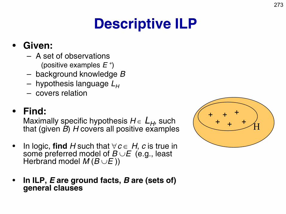
273
Descriptive ILP
• Given: – A set of observations
(positive examples E +)
– background knowledge B
– hypothesis language LH
– covers relation
• Find: Maximally specific hypothesis H LH, such that (given B) H covers all positive examples
• In logic, find H such that c H, c is true in some preferred model of B E (e.g., least Herbrand model M (B E ))
• In ILP, E are ground facts, B are (sets of) general clauses
+ + + + + +
H
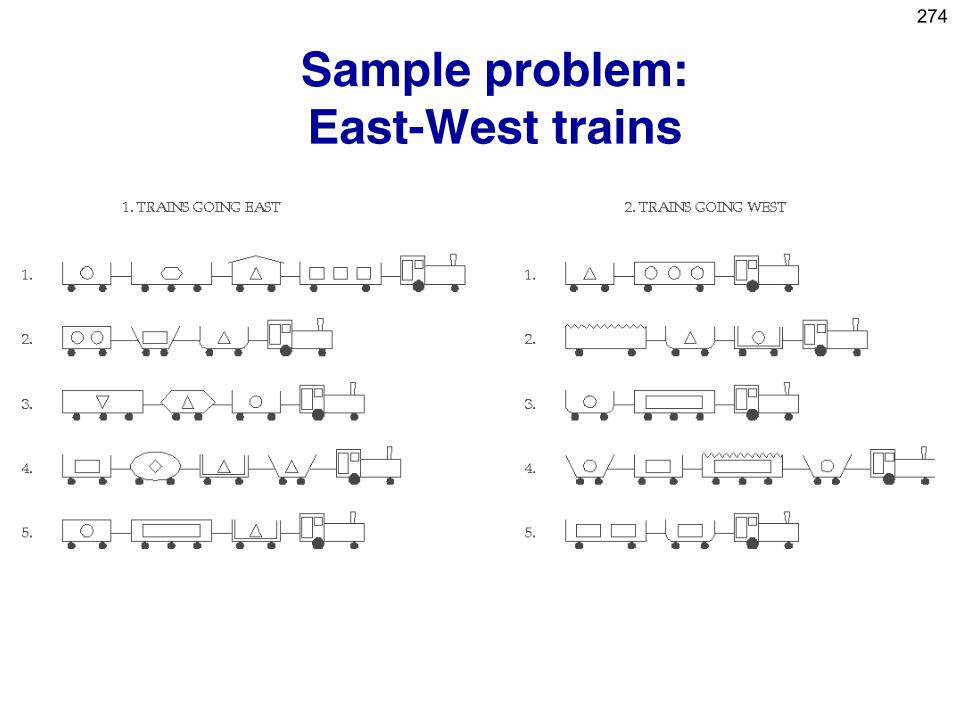
274
Sample problem:
East-West trains
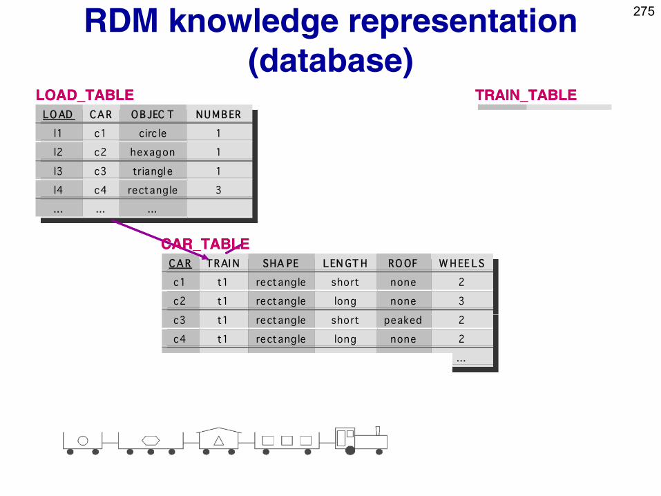
275
RDM knowledge representation
(database)
TRAI N EAS TB OU ND
t1 TRU E
t2 TRU E
… …
t6 FAL SE
… …
TRAIN_TABLE TRAIN_TABLE
CA R TRAI N SHA PE LEN GT H RO OF W H EE LS
c1 t1 rectang le short none 2
c2 t1 rectang le long none 3
c3 t1 rectang le short peaked 2
c4 t1 rectang le long none 2
… … … …
LO AD CA R O B JEC T NU M B ER
l1 c1 circ le 1
l2 c2 hexagon 1
l3 c3 triangl e 1
l4 c4 rectang le 3
… … …
LOAD_TABLE LOAD_TABLE
CAR_TABLE CAR_TABLE
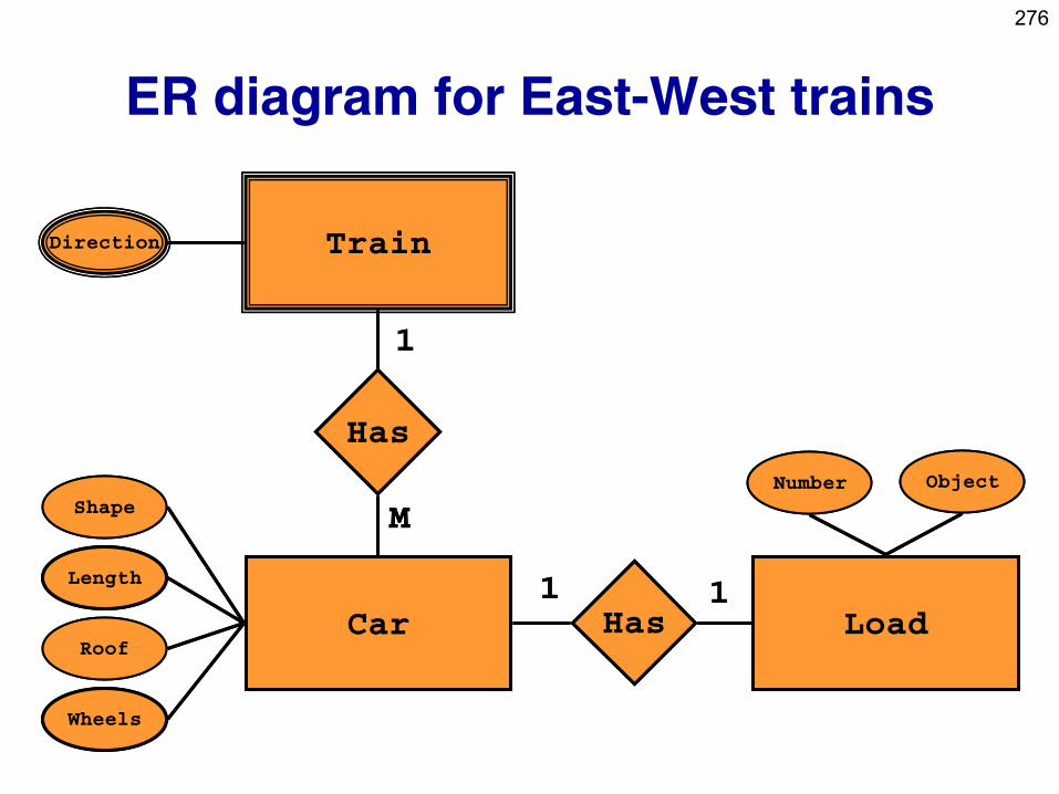
276
ER diagram for East-West trains
Train Direction Direction
Has Has
Car
Shape
Length
Roof
Wheels
1 1
M M
Has Has Load 1 1 1 1
Number Object
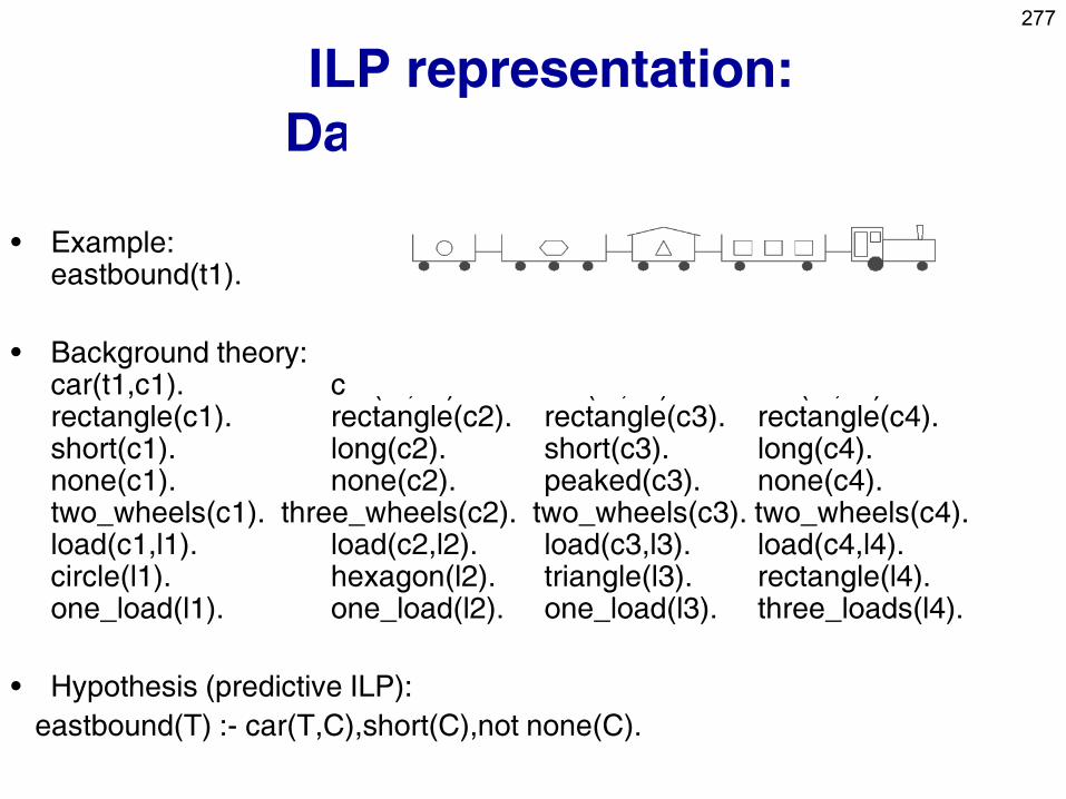
277
ILP representation:
Datalog ground facts
• Example: eastbound(t1).
• Background theory: car(t1,c1). car(t1,c2). car(t1,c3). car(t1,c4). rectangle(c1). rectangle(c2). rectangle(c3). rectangle(c4). short(c1). long(c2). short(c3). long(c4). none(c1). none(c2). peaked(c3). none(c4). two_wheels(c1). three_wheels(c2). two_wheels(c3). two_wheels(c4). load(c1,l1). load(c2,l2). load(c3,l3). load(c4,l4). circle(l1). hexagon(l2). triangle(l3). rectangle(l4). one_load(l1). one_load(l2). one_load(l3). three_loads(l4).
• Hypothesis (predictive ILP):
eastbound(T) :- car(T,C),short(C),not none(C).

278
ILP representation:
Datalog ground clauses
• Example: eastbound(t1):- car(t1,c1),rectangle(c1),short(c1),none(c1),two_wheels(c1), load(c1,l1),circle(l1),one_load(l1), car(t1,c2),rectangle(c2),long(c2),none(c2),three_wheels(c2), load(c2,l2),hexagon(l2),one_load(l2), car(t1,c3),rectangle(c3),short(c3),peaked(c3),two_wheels(c3), load(c3,l3),triangle(l3),one_load(l3), car(t1,c4),rectangle(c4),long(c4),none(c4),two_wheels(c4), load(c4,l4),rectangle(l4),three_load(l4).
• Background theory: empty
• Hypothesis: eastbound(T):-car(T,C),short(C),not none(C).
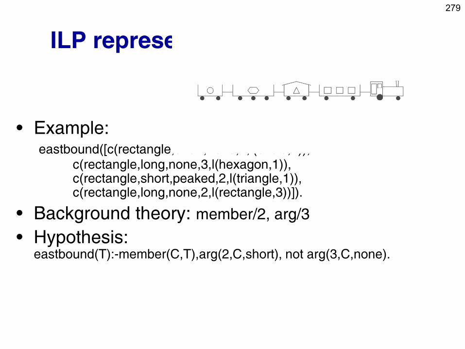
279
ILP representation: Prolog terms
• Example: eastbound([c(rectangle,short,none,2,l(circle,1)),
c(rectangle,long,none,3,l(hexagon,1)), c(rectangle,short,peaked,2,l(triangle,1)), c(rectangle,long,none,2,l(rectangle,3))]).
• Background theory: member/2, arg/3
• Hypothesis: eastbound(T):-member(C,T),arg(2,C,short), not arg(3,C,none).
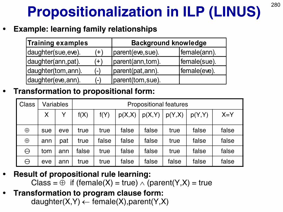
280
Propositionalization in ILP (LINUS) • Example: learning family relationships
• Transformation to propositional form:
• Result of propositional rule learning: Class = if (female(X) = true) (parent(Y,X) = true
• Transformation to program clause form: daughter(X,Y) female(X),parent(Y,X)
Training examples
daughter(sue,eve). (+) parent(eve,sue). female(ann).
daughter(ann,pat). (+) parent(ann,tom). female(sue).
daughter(tom,ann). (-) parent(pat,ann). female(eve).
daughter(eve,ann). (-) parent(tom,sue).
Background knowledge
Class Variables Propositional features
X Y f(X) f(Y) p(X,X) p(X,Y) p(Y,X) p(Y,Y) X=Y
sue eve true true false false true false false
ann pat true false false false true false false
tom ann false true false false true false false
eve ann true true false false false false false
281
First-order feature construction
• All the expressiveness of ILP is in the features
• Given a way to construct (or choose) first-order
features, body construction in ILP becomes
propositional
– idea: learn non-determinate clauses with LINUS by
saturating background knowledge (performing
systematic feature construction in a given language bias)
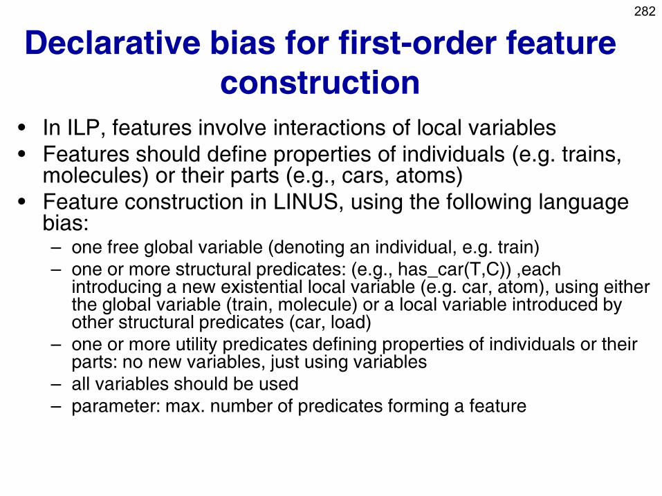
282
Declarative bias for first-order feature
construction
• In ILP, features involve interactions of local variables
• Features should define properties of individuals (e.g. trains, molecules) or their parts (e.g., cars, atoms)
• Feature construction in LINUS, using the following language bias: – one free global variable (denoting an individual, e.g. train)
– one or more structural predicates: (e.g., has_car(T,C)) ,each introducing a new existential local variable (e.g. car, atom), using either the global variable (train, molecule) or a local variable introduced by other structural predicates (car, load)
– one or more utility predicates defining properties of individuals or their parts: no new variables, just using variables
– all variables should be used
– parameter: max. number of predicates forming a feature
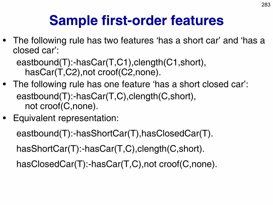
283
Sample first-order features
• The following rule has two features ‘has a short car’ and ‘has a closed car’:
eastbound(T):-hasCar(T,C1),clength(C1,short), hasCar(T,C2),not croof(C2,none).
• The following rule has one feature ‘has a short closed car’:
eastbound(T):-hasCar(T,C),clength(C,short), not croof(C,none).
• Equivalent representation:
eastbound(T):-hasShortCar(T),hasClosedCar(T).
hasShortCar(T):-hasCar(T,C),clength(C,short).
hasClosedCar(T):-hasCar(T,C),not croof(C,none).
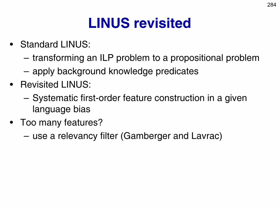
284
LINUS revisited
• Standard LINUS:
– transforming an ILP problem to a propositional problem
– apply background knowledge predicates
• Revisited LINUS:
– Systematic first-order feature construction in a given
language bias
• Too many features?
– use a relevancy filter (Gamberger and Lavrac)
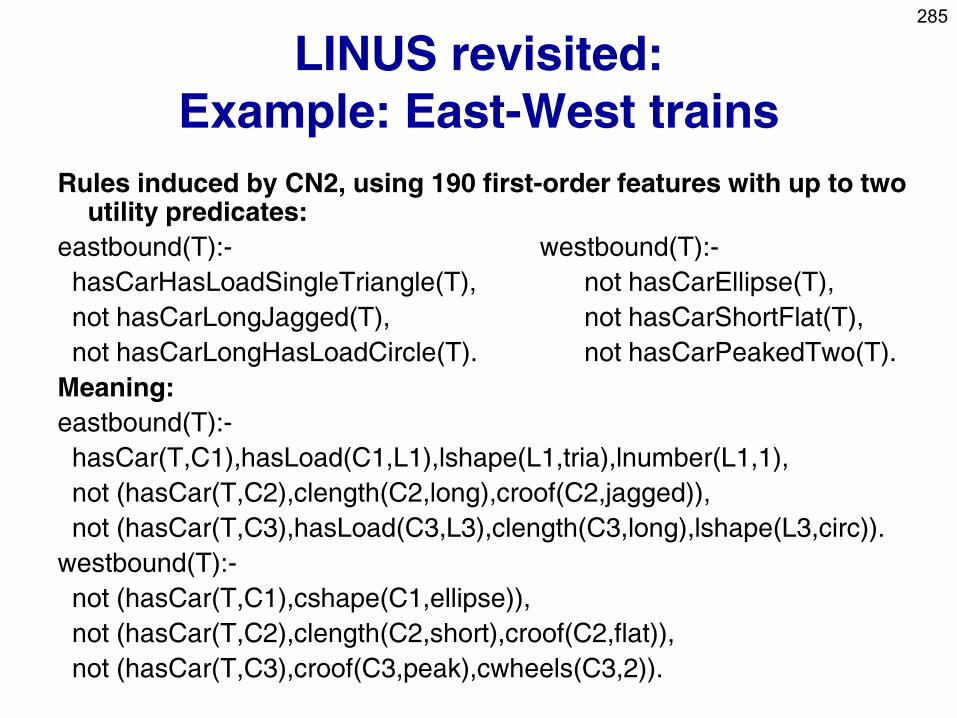
285
LINUS revisited:
Example: East-West trains
Rules induced by CN2, using 190 first-order features with up to two utility predicates:
eastbound(T):- westbound(T):-
hasCarHasLoadSingleTriangle(T), not hasCarEllipse(T),
not hasCarLongJagged(T), not hasCarShortFlat(T),
not hasCarLongHasLoadCircle(T). not hasCarPeakedTwo(T).
Meaning:
eastbound(T):-
hasCar(T,C1),hasLoad(C1,L1),lshape(L1,tria),lnumber(L1,1),
not (hasCar(T,C2),clength(C2,long),croof(C2,jagged)),
not (hasCar(T,C3),hasLoad(C3,L3),clength(C3,long),lshape(L3,circ)).
westbound(T):-
not (hasCar(T,C1),cshape(C1,ellipse)),
not (hasCar(T,C2),clength(C2,short),croof(C2,flat)),
not (hasCar(T,C3),croof(C3,peak),cwheels(C3,2)).
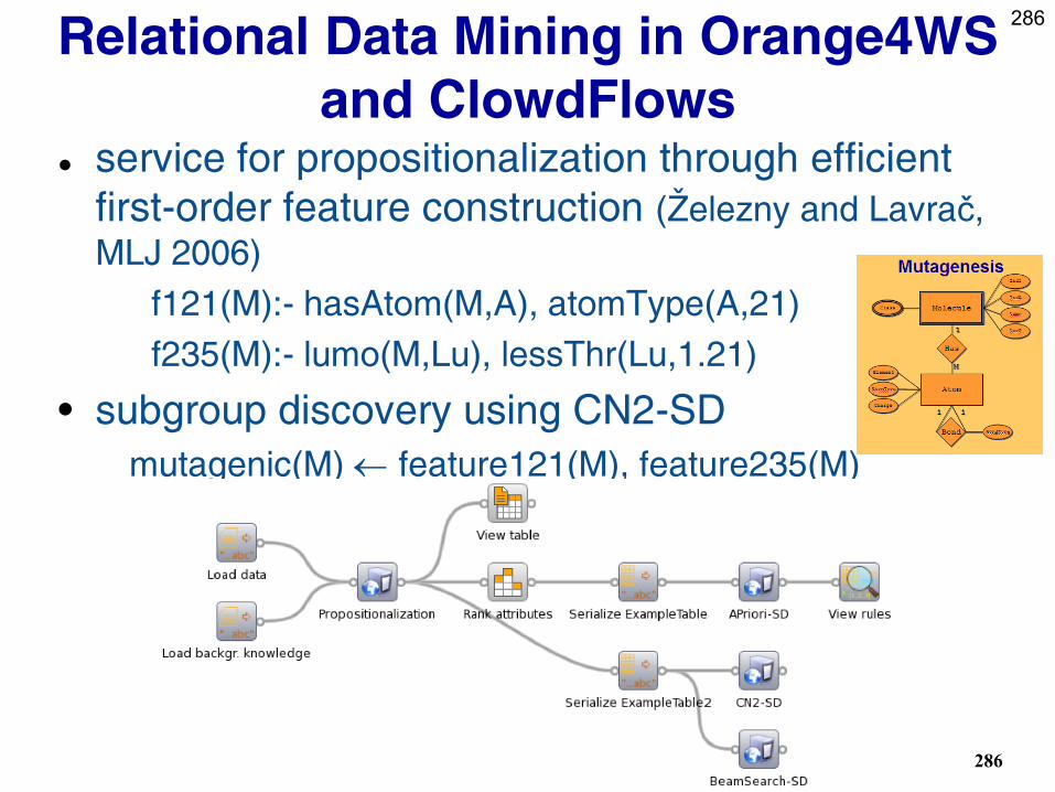
286
286
Relational Data Mining in Orange4WS
and ClowdFlows service for propositionalization through efficient
first-order feature construction (Železny and Lavrač,
MLJ 2006)
f121(M):- hasAtom(M,A), atomType(A,21)
f235(M):- lumo(M,Lu), lessThr(Lu,1.21)
• subgroup discovery using CN2-SD
mutagenic(M) feature121(M), feature235(M)
287
Part V:
Relational Data Mining
• What is RDM
• Propositionalization techniques
• Semantic Data Mining
• Inductive Logic programming
• Learning as search in Inductive Logic
Programming
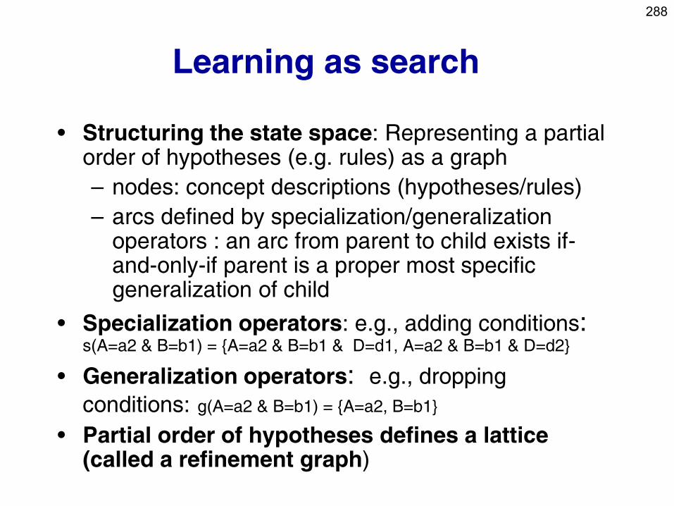
288
Learning as search
• Structuring the state space: Representing a partial order of hypotheses (e.g. rules) as a graph
– nodes: concept descriptions (hypotheses/rules)
– arcs defined by specialization/generalization operators : an arc from parent to child exists if-and-only-if parent is a proper most specific generalization of child
• Specialization operators: e.g., adding conditions: s(A=a2 & B=b1) = {A=a2 & B=b1 & D=d1, A=a2 & B=b1 & D=d2}
• Generalization operators: e.g., dropping
conditions: g(A=a2 & B=b1) = {A=a2, B=b1}
• Partial order of hypotheses defines a lattice (called a refinement graph)
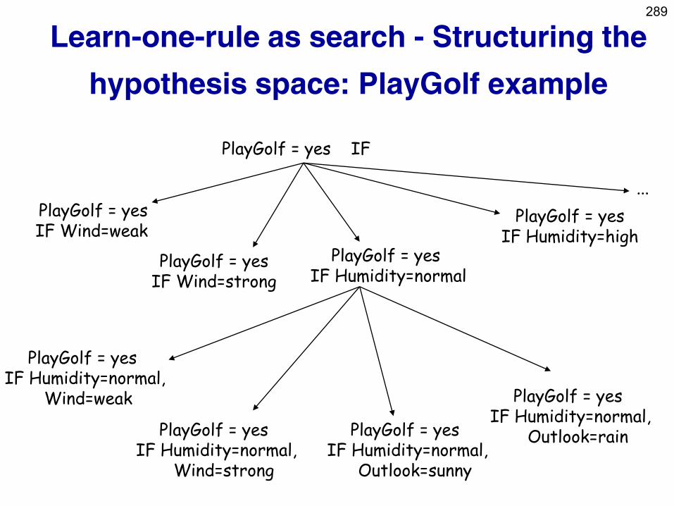
289
Learn-one-rule as search - Structuring the
hypothesis space: PlayGolf example
PlayGolf = yes IF
PlayGolf = yes IF Wind=weak
PlayGolf = yes IF Wind=strong
PlayGolf = yes IF Humidity=normal
PlayGolf = yes IF Humidity=high
PlayGolf = yes IF Humidity=normal,
Wind=weak
PlayGolf = yes IF Humidity=normal,
Wind=strong
PlayGolf = yes IF Humidity=normal,
Outlook=sunny
PlayGolf = yes IF Humidity=normal,
Outlook=rain
...
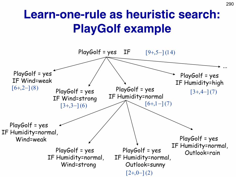
290
Learn-one-rule as heuristic search:
PlayGolf example
PlayGolf = yes IF
PlayGolf = yes IF Wind=weak
PlayGolf = yes IF Wind=strong
PlayGolf = yes IF Humidity=normal
PlayGolf = yes IF Humidity=high
PlayGolf = yes IF Humidity=normal,
Wind=weak
PlayGolf = yes IF Humidity=normal,
Wind=strong
PlayGolf = yes IF Humidity=normal,
Outlook=sunny
PlayGolf = yes IF Humidity=normal,
Outlook=rain
[9,5] (14)
[6,2] (8)
[3,3] (6) [6,1] (7)
[3,4] (7)
...
[2,0] (2)
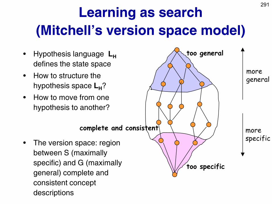
291
Learning as search
(Mitchell’s version space model)
• Hypothesis language LH
defines the state space
• How to structure the
hypothesis space LH?
• How to move from one
hypothesis to another?
• The version space: region
between S (maximally
specific) and G (maximally
general) complete and
consistent concept
descriptions
too general
too specific
more general
more specific
complete and consistent
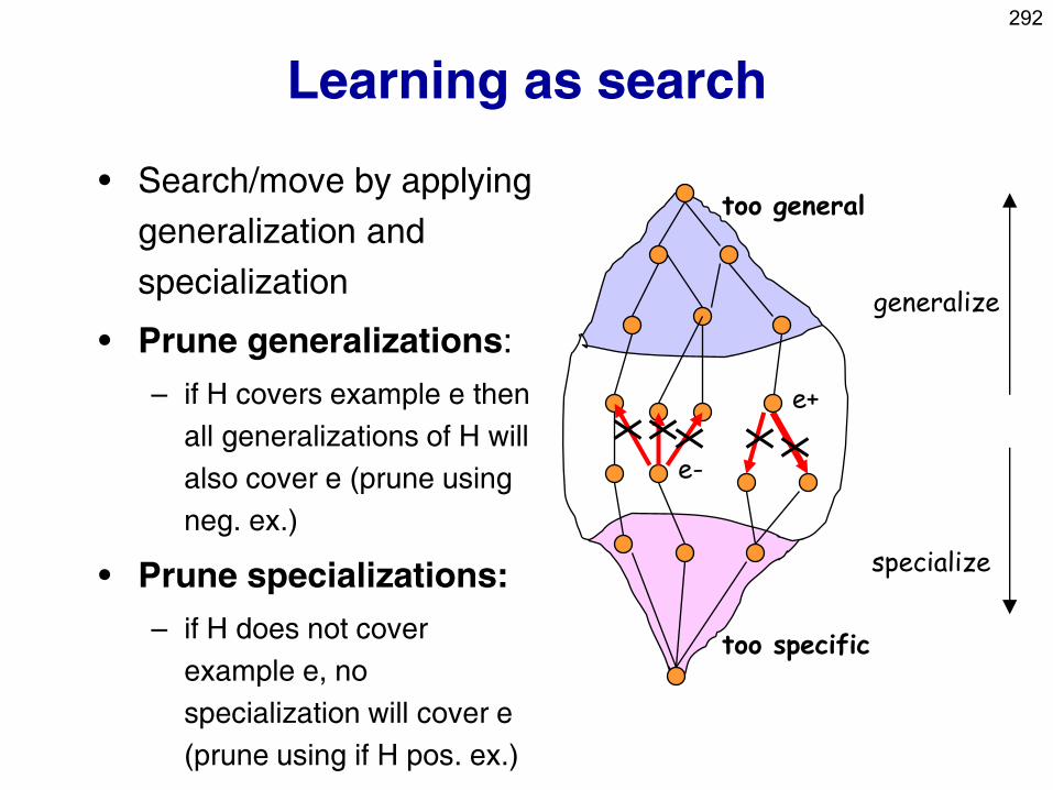
292
Learning as search
• Search/move by applying
generalization and
specialization
• Prune generalizations:
– if H covers example e then
all generalizations of H will
also cover e (prune using
neg. ex.)
• Prune specializations:
– if H does not cover
example e, no
specialization will cover e
(prune using if H pos. ex.)
too general
too specific
generalize
specialize
e-
e+
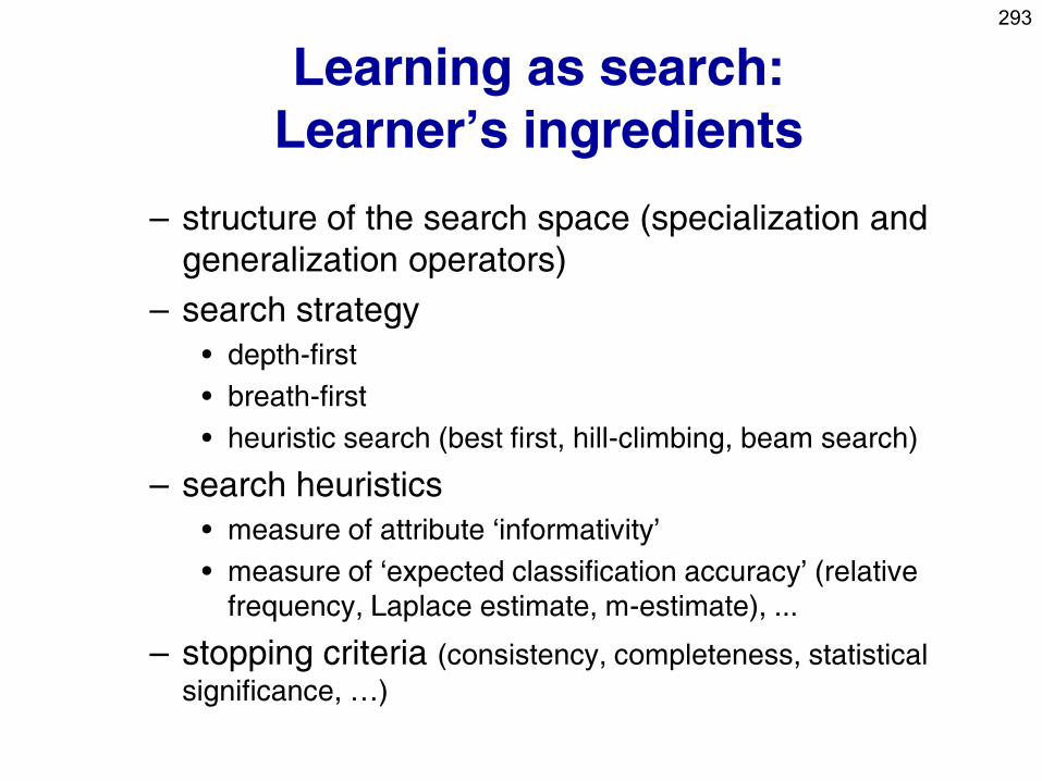
293
Learning as search:
Learner’s ingredients
– structure of the search space (specialization and
generalization operators)
– search strategy
• depth-first
• breath-first
• heuristic search (best first, hill-climbing, beam search)
– search heuristics
• measure of attribute ‘informativity’
• measure of ‘expected classification accuracy’ (relative
frequency, Laplace estimate, m-estimate), ...
– stopping criteria (consistency, completeness, statistical
significance, …)
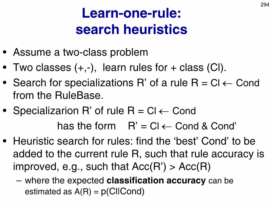
294
Learn-one-rule:
search heuristics
• Assume a two-class problem
• Two classes (+,-), learn rules for + class (Cl).
• Search for specializations R’ of a rule R = Cl Cond
from the RuleBase.
• Specializarion R’ of rule R = Cl Cond
has the form R’ = Cl Cond & Cond’
• Heuristic search for rules: find the ‘best’ Cond’ to be
added to the current rule R, such that rule accuracy is
improved, e.g., such that Acc(R’) > Acc(R)
– where the expected classification accuracy can be
estimated as A(R) = p(Cl|Cond)
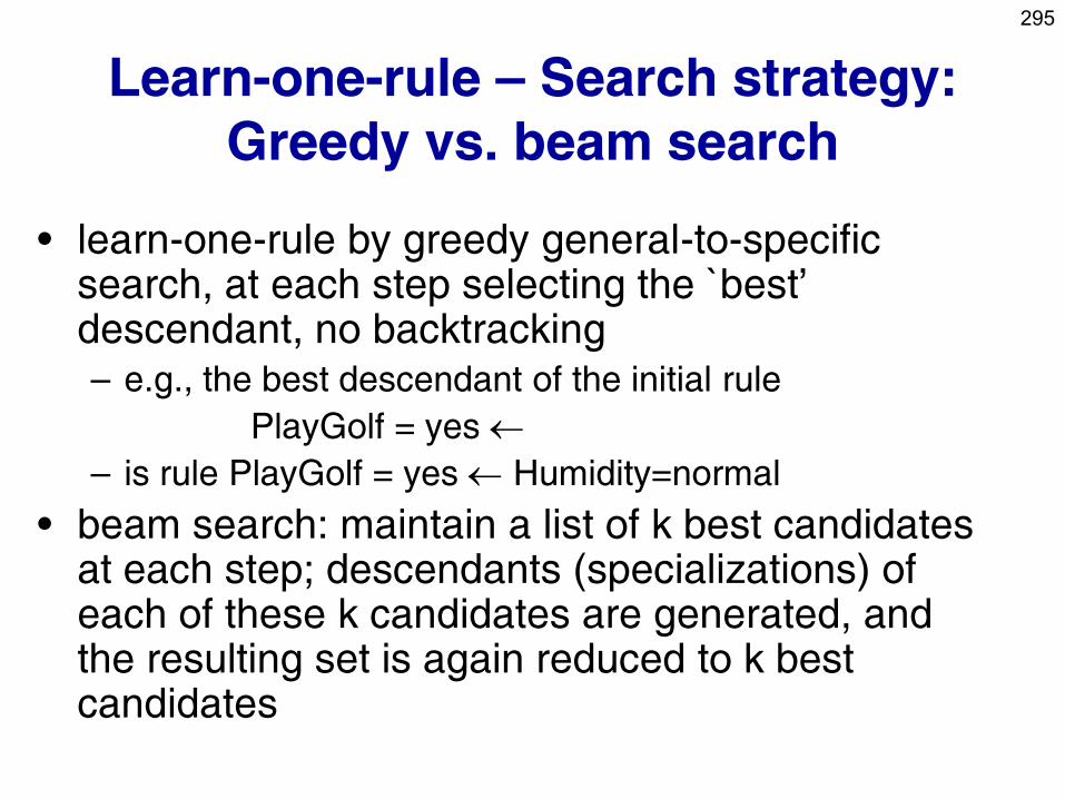
295
Learn-one-rule – Search strategy:
Greedy vs. beam search
• learn-one-rule by greedy general-to-specific search, at each step selecting the `best’ descendant, no backtracking – e.g., the best descendant of the initial rule
PlayGolf = yes
– is rule PlayGolf = yes Humidity=normal
• beam search: maintain a list of k best candidates at each step; descendants (specializations) of each of these k candidates are generated, and the resulting set is again reduced to k best candidates
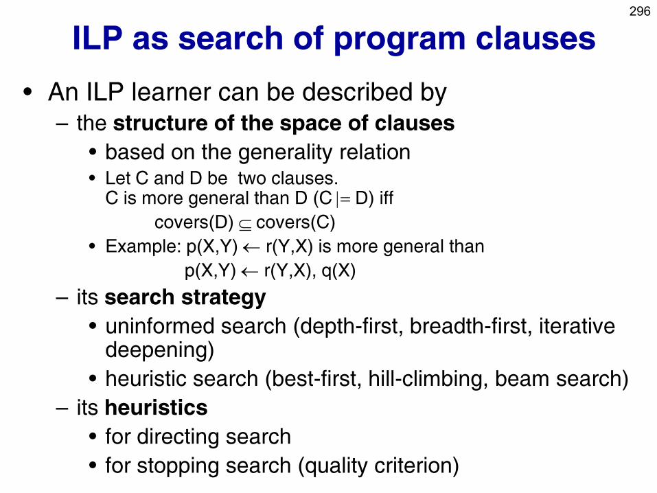
296
ILP as search of program clauses
• An ILP learner can be described by – the structure of the space of clauses
• based on the generality relation • Let C and D be two clauses.
C is more general than D (C | D) iff
covers(D) covers(C)
• Example: p(X,Y) r(Y,X) is more general than
p(X,Y) r(Y,X), q(X)
– its search strategy
• uninformed search (depth-first, breadth-first, iterative deepening)
• heuristic search (best-first, hill-climbing, beam search)
– its heuristics
• for directing search
• for stopping search (quality criterion)
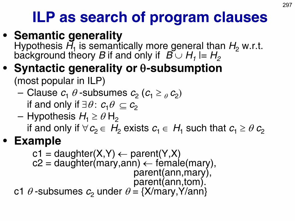
297
• Semantic generality Hypothesis H1 is semantically more general than H2 w.r.t. background theory B if and only if B H1 |= H2
• Syntactic generality or -subsumption
(most popular in ILP)
– Clause c1 -subsumes c2 (c1 c2)
if and only if : c1 c2
– Hypothesis H1 H2
if and only if c2 H2 exists c1 H1 such that c1 c2
• Example c1 = daughter(X,Y) parent(Y,X)
c2 = daughter(mary,ann) female(mary), parent(ann,mary), parent(ann,tom). c1 -subsumes c2 under = {X/mary,Y/ann}
ILP as search of program clauses
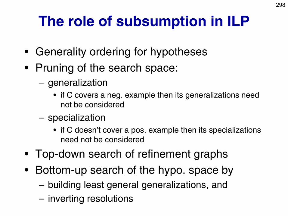
298
The role of subsumption in ILP
• Generality ordering for hypotheses
• Pruning of the search space:
– generalization
• if C covers a neg. example then its generalizations need
not be considered
– specialization
• if C doesn’t cover a pos. example then its specializations
need not be considered
• Top-down search of refinement graphs
• Bottom-up search of the hypo. space by
– building least general generalizations, and
– inverting resolutions
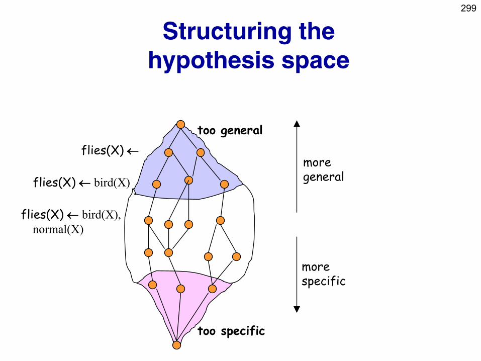
299
Structuring the
hypothesis space
too general
too specific
more general
more specific
flies(X)
flies(X) bird(X),
normal(X)
flies(X) bird(X)
300
Two strategies for learning
• General-to-specific
– if -subsumption is used then refinement
operators
• Specific-to-general search
– if -subsumption is used then lgg-operator or
generalization operator
301
• Two strategies for learning
– Top-down search of refinement graphs
– Bottom-up search
• building least general generalizations
• inverting resolution (CIGOL)
• inverting entailment (PROGOL)
ILP as search of program clauses
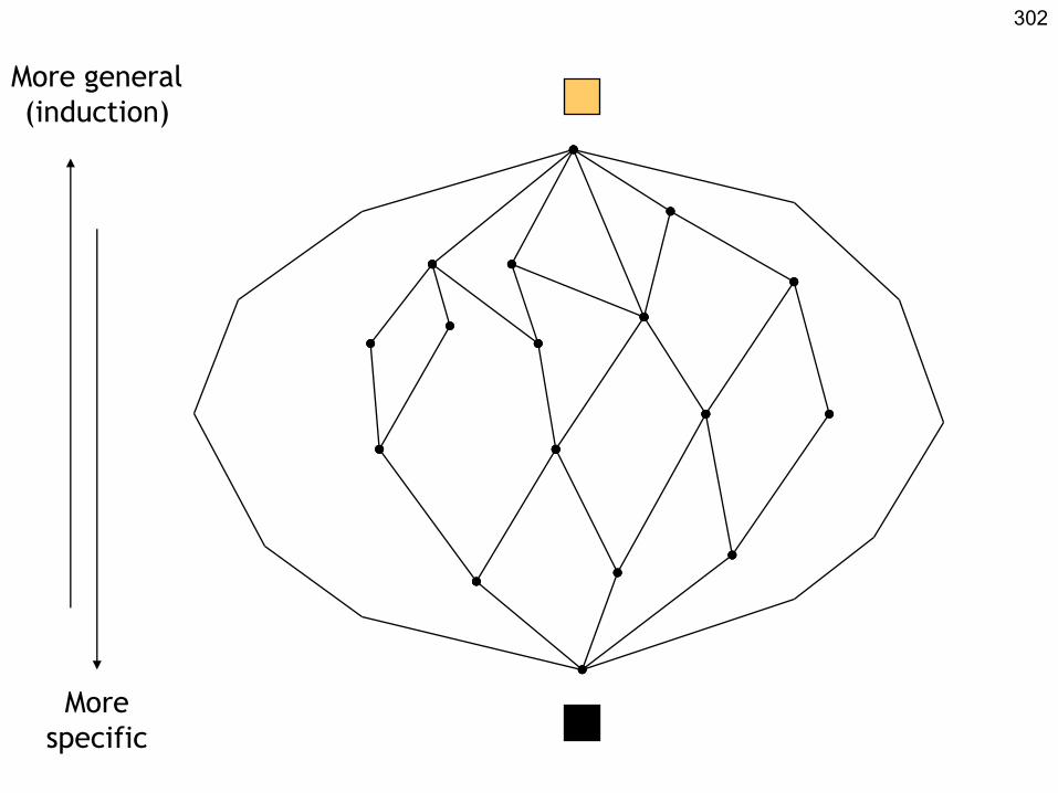
302
More general
(induction)
More
specific
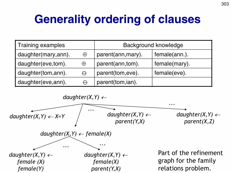
303
Generality ordering of clauses
Training examples Background knowledge
daughter(mary,ann). parent(ann,mary). female(ann.).
daughter(eve,tom). parent(ann,tom). female(mary).
daughter(tom,ann). parent(tom,eve). female(eve).
daughter(eve,ann). parent(tom,ian).
daughter(X,Y)
daughter(X,Y) X=Y daughter(X,Y)
parent(Y,X)
daughter(X,Y)
parent(X,Z)
daughter(X,Y) female(X)
daughter(X,Y)
female (X)
female(Y)
daughter(X,Y)
female(X)
parent(Y,X)
... ...
... ...
Part of the refinement
graph for the family
relations problem.
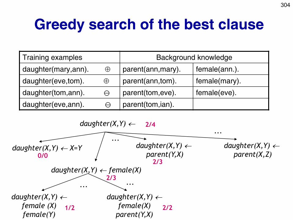
304
Greedy search of the best clause
daughter(X,Y)
daughter(X,Y) X=Y daughter(X,Y)
parent(Y,X)
daughter(X,Y)
parent(X,Z)
daughter(X,Y) female(X)
daughter(X,Y)
female (X)
female(Y)
daughter(X,Y)
female(X)
parent(Y,X)
... ...
... ...
2/4
0/0 2/3
2/3
1/2 2/2
Training examples Background knowledge
daughter(mary,ann). parent(ann,mary). female(ann.).
daughter(eve,tom). parent(ann,tom). female(mary).
daughter(tom,ann). parent(tom,eve). female(eve).
daughter(eve,ann). parent(tom,ian).
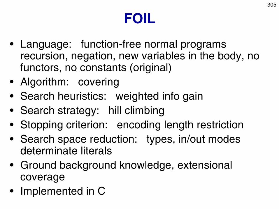
305
FOIL
• Language: function-free normal programs recursion, negation, new variables in the body, no functors, no constants (original)
• Algorithm: covering
• Search heuristics: weighted info gain
• Search strategy: hill climbing
• Stopping criterion: encoding length restriction
• Search space reduction: types, in/out modes determinate literals
• Ground background knowledge, extensional coverage
• Implemented in C
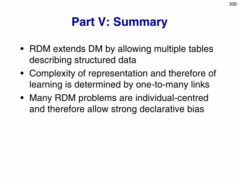
306
Part V: Summary
• RDM extends DM by allowing multiple tables
describing structured data
• Complexity of representation and therefore of
learning is determined by one-to-many links
• Many RDM problems are individual-centred
and therefore allow strong declarative bias
Advanced Topics
• Text mining: An introduction
• Document clustering and outlier detection
• Wordification approach to relational data mining
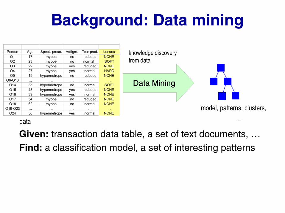
Background: Data mining
data
knowledge discovery
from data
model, patterns, clusters,
…
Given: transaction data table, a set of text documents, …
Find: a classification model, a set of interesting patterns
Data MiningData Mining
Person Age Spect. presc. Astigm. Tear prod. Lenses
O1 17 myope no reduced NONE
O2 23 myope no normal SOFT
O3 22 myope yes reduced NONE
O4 27 myope yes normal HARD
O5 19 hypermetrope no reduced NONE
O6-O13 ... ... ... ... ...
O14 35 hypermetrope no normal SOFT
O15 43 hypermetrope yes reduced NONE
O16 39 hypermetrope yes normal NONE
O17 54 myope no reduced NONE
O18 62 myope no normal NONE
O19-O23 ... ... ... ... ...
O24 56 hypermetrope yes normal NONE
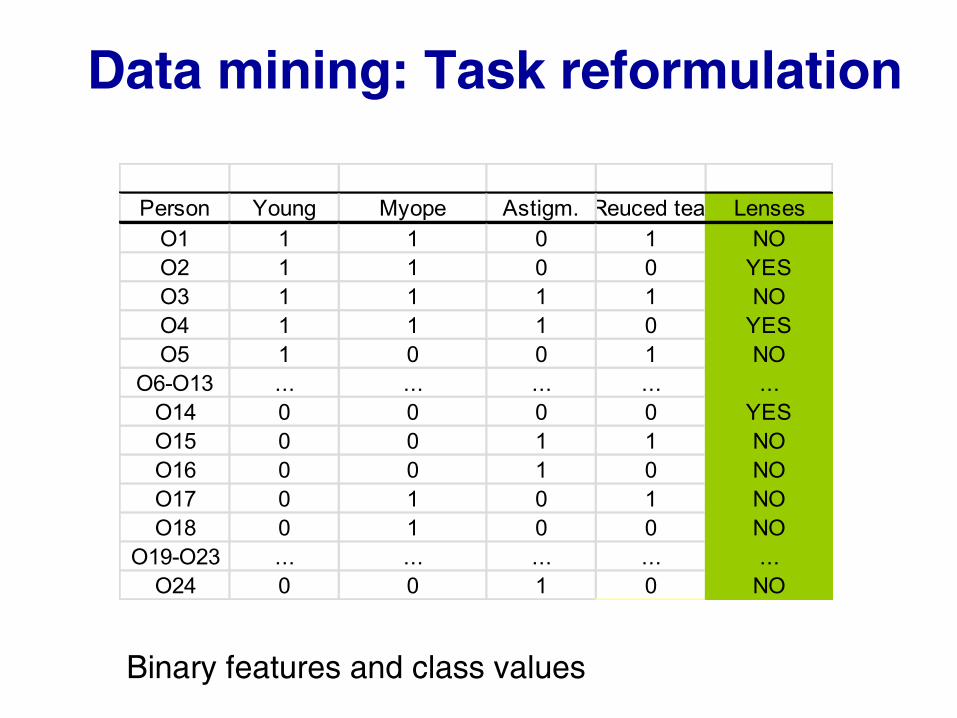
Data mining: Task reformulation
Person Young Myope Astigm. Reuced tear Lenses
O1 1 1 0 1 NO
O2 1 1 0 0 YES
O3 1 1 1 1 NO
O4 1 1 1 0 YES
O5 1 0 0 1 NO
O6-O13 ... ... ... ... ...
O14 0 0 0 0 YES
O15 0 0 1 1 NO
O16 0 0 1 0 NO
O17 0 1 0 1 NO
O18 0 1 0 0 NO
O19-O23 ... ... ... ... ...
O24 0 0 1 0 NO
Binary features and class values
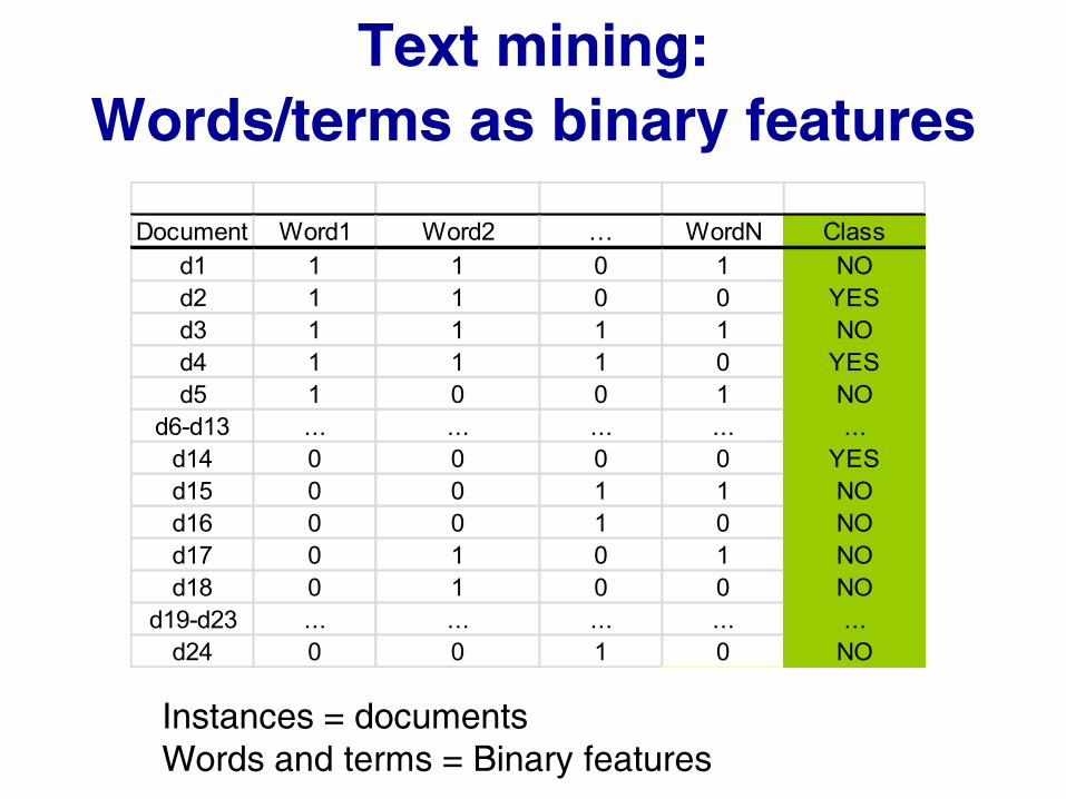
Text mining:
Words/terms as binary features
Instances = documents
Words and terms = Binary features
Document Word1 Word2 … WordN Class
d1 1 1 0 1 NO
d2 1 1 0 0 YES
d3 1 1 1 1 NO
d4 1 1 1 0 YES
d5 1 0 0 1 NO
d6-d13 ... ... ... ... ...
d14 0 0 0 0 YES
d15 0 0 1 1 NO
d16 0 0 1 0 NO
d17 0 1 0 1 NO
d18 0 1 0 0 NO
d19-d23 ... ... ... ... ...
d24 0 0 1 0 NO
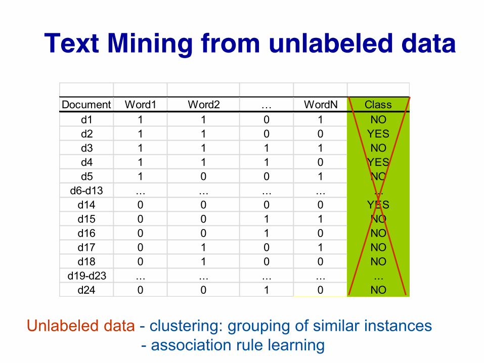
Text Mining from unlabeled data
Unlabeled data - clustering: grouping of similar instances
- association rule learning
Document Word1 Word2 … WordN Class
d1 1 1 0 1 NO
d2 1 1 0 0 YES
d3 1 1 1 1 NO
d4 1 1 1 0 YES
d5 1 0 0 1 NO
d6-d13 ... ... ... ... ...
d14 0 0 0 0 YES
d15 0 0 1 1 NO
d16 0 0 1 0 NO
d17 0 1 0 1 NO
d18 0 1 0 0 NO
d19-d23 ... ... ... ... ...
d24 0 0 1 0 NO
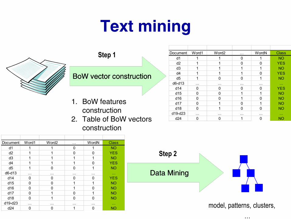
Text mining
BoWBoW vector constructionvector construction
model, patterns, clusters,
…
Data MiningData Mining
Step 1
Step 2
1. BoW features
construction
2. Table of BoW vectors
construction
Document Word1 Word2 … WordN Class
d1 1 1 0 1 NO
d2 1 1 0 0 YES
d3 1 1 1 1 NO
d4 1 1 1 0 YES
d5 1 0 0 1 NO
d6-d13 ... ... ... ... ...
d14 0 0 0 0 YES
d15 0 0 1 1 NO
d16 0 0 1 0 NO
d17 0 1 0 1 NO
d18 0 1 0 0 NO
d19-d23 ... ... ... ... ...
d24 0 0 1 0 NO
Document Word1 Word2 … WordN Class
d1 1 1 0 1 NO
d2 1 1 0 0 YES
d3 1 1 1 1 NO
d4 1 1 1 0 YES
d5 1 0 0 1 NO
d6-d13 ... ... ... ... ...
d14 0 0 0 0 YES
d15 0 0 1 1 NO
d16 0 0 1 0 NO
d17 0 1 0 1 NO
d18 0 1 0 0 NO
d19-d23 ... ... ... ... ...
d24 0 0 1 0 NO
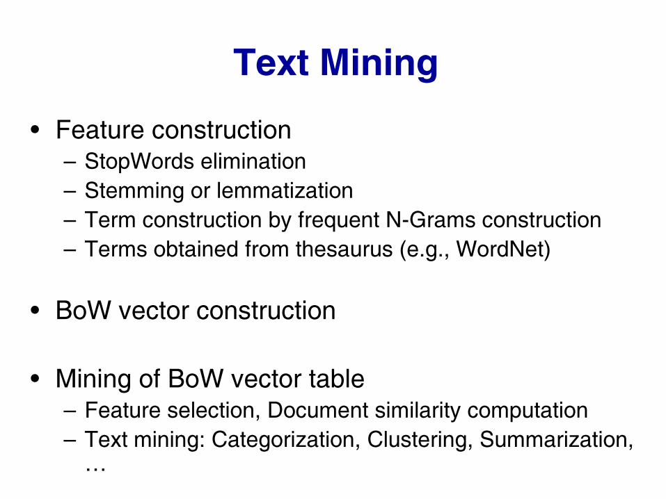
Text Mining
• Feature construction – StopWords elimination
– Stemming or lemmatization
– Term construction by frequent N-Grams construction
– Terms obtained from thesaurus (e.g., WordNet)
• BoW vector construction
• Mining of BoW vector table – Feature selection, Document similarity computation
– Text mining: Categorization, Clustering, Summarization, …
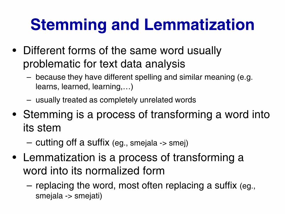
Stemming and Lemmatization
• Different forms of the same word usually
problematic for text data analysis – because they have different spelling and similar meaning (e.g.
learns, learned, learning,…)
– usually treated as completely unrelated words
• Stemming is a process of transforming a word into
its stem
– cutting off a suffix (eg., smejala -> smej)
• Lemmatization is a process of transforming a
word into its normalized form
– replacing the word, most often replacing a suffix (eg.,
smejala -> smejati)
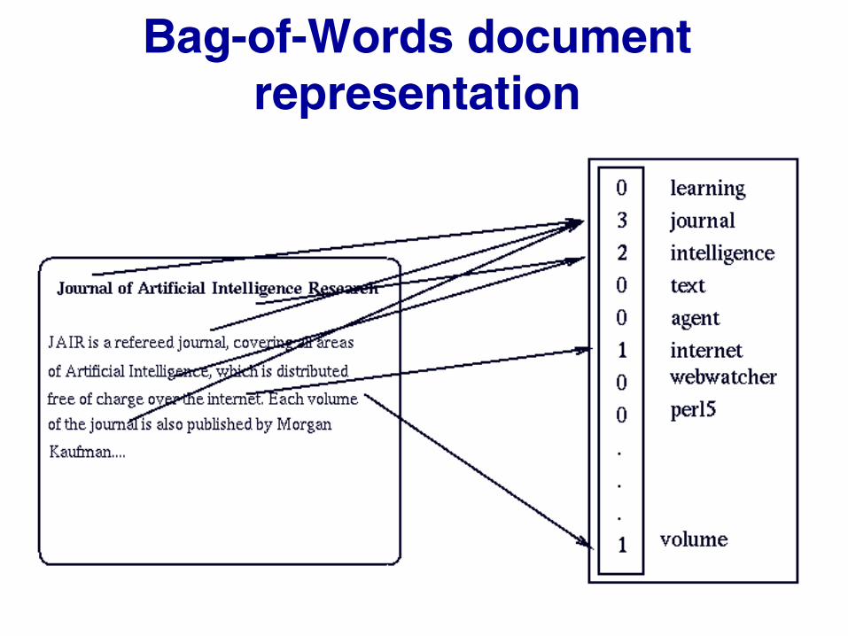
Bag-of-Words document
representation
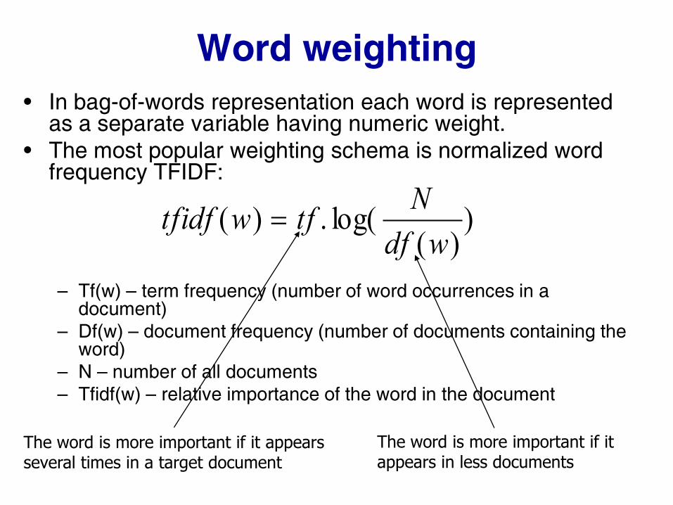
Word weighting
• In bag-of-words representation each word is represented as a separate variable having numeric weight.
• The most popular weighting schema is normalized word frequency TFIDF:
– Tf(w) – term frequency (number of word occurrences in a
document)
– Df(w) – document frequency (number of documents containing the word)
– N – number of all documents
– Tfidf(w) – relative importance of the word in the document
))(
log(.)(wdf
Ntfwtfidf
The word is more important if it appears several times in a target document
The word is more important if it appears in less documents
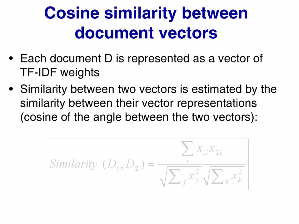
Cosine similarity between
document vectors
• Each document D is represented as a vector of
TF-IDF weights
• Similarity between two vectors is estimated by the
similarity between their vector representations
(cosine of the angle between the two vectors):
Advanced Topics
• Text mining: An introduction
• Document clustering and outlier detection
• Wordification approach to relational data mining
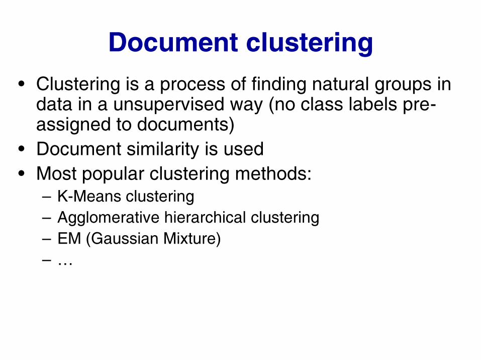
Document clustering
• Clustering is a process of finding natural groups in data in a unsupervised way (no class labels pre-assigned to documents)
• Document similarity is used
• Most popular clustering methods: – K-Means clustering
– Agglomerative hierarchical clustering
– EM (Gaussian Mixture)
– …
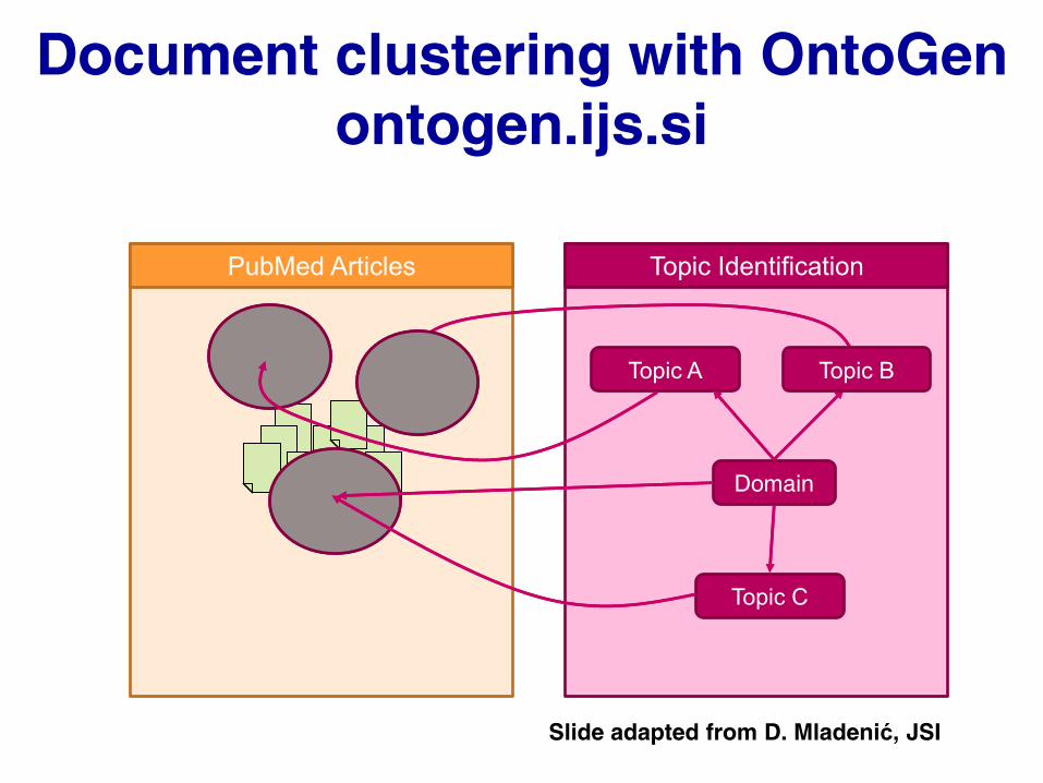
Document clustering with OntoGen
ontogen.ijs.si
Domain
PubMed Articles Topic Identification
Topic A Topic B
Topic C
Slide adapted from D. Mladenić, JSI
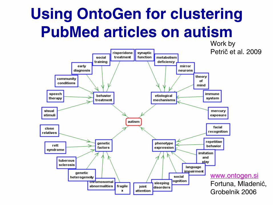
Using OntoGen for clustering
PubMed articles on autism
www.ontogen.si
Fortuna, Mladenić,
Grobelnik 2006
Work by
Petrič et al. 2009
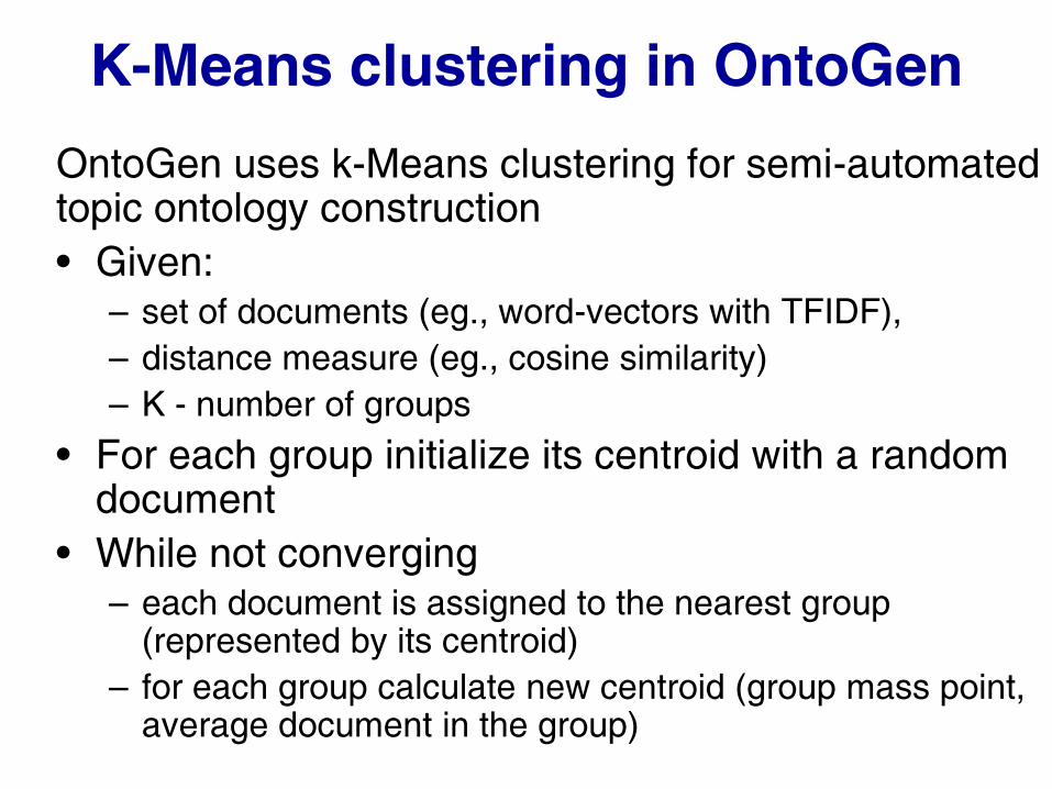
K-Means clustering in OntoGen
OntoGen uses k-Means clustering for semi-automated topic ontology construction
• Given: – set of documents (eg., word-vectors with TFIDF),
– distance measure (eg., cosine similarity)
– K - number of groups
• For each group initialize its centroid with a random document
• While not converging – each document is assigned to the nearest group
(represented by its centroid)
– for each group calculate new centroid (group mass point, average document in the group)
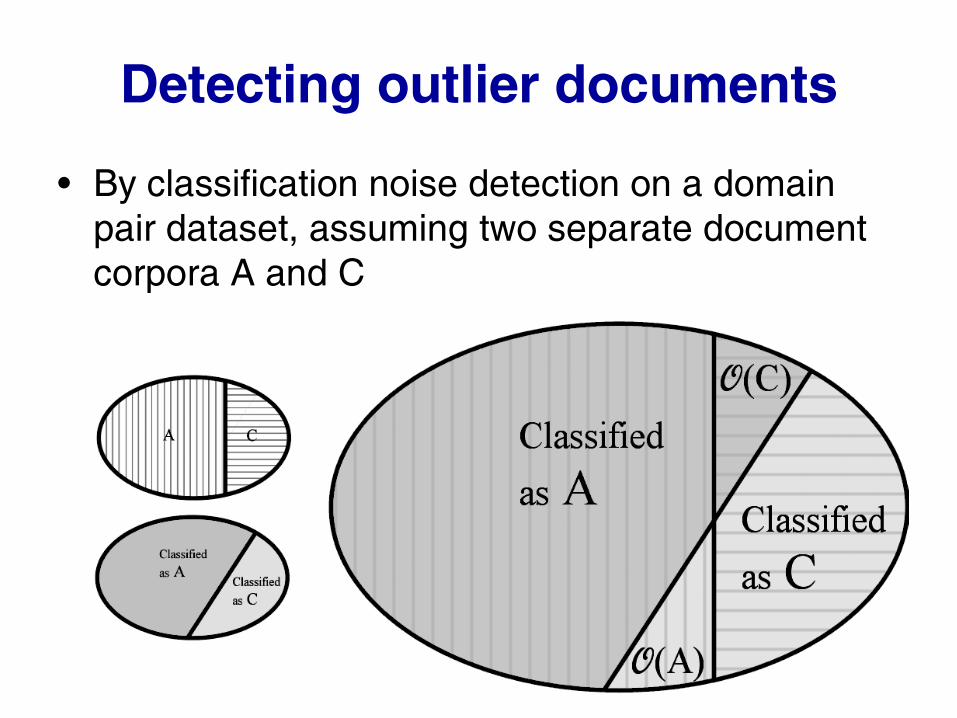
Detecting outlier documents
• By classification noise detection on a domain
pair dataset, assuming two separate document
corpora A and C
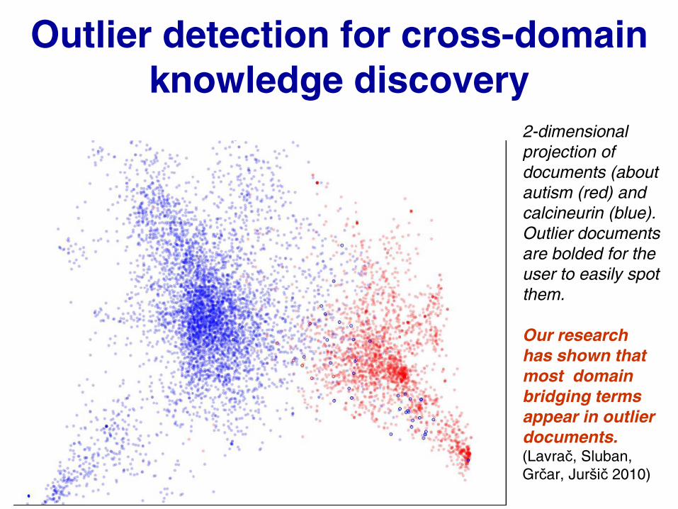
Outlier detection for cross-domain
knowledge discovery
2-dimensional
projection of
documents (about
autism (red) and
calcineurin (blue).
Outlier documents
are bolded for the
user to easily spot
them.
Our research
has shown that
most domain
bridging terms
appear in outlier
documents. (Lavrač, Sluban,
Grčar, Juršič 2010)
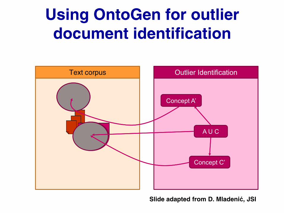
Using OntoGen for outlier
document identification
A U C
Text corpus Outlier Identification
Concept A’
Concept C’
Slide adapted from D. Mladenić, JSI
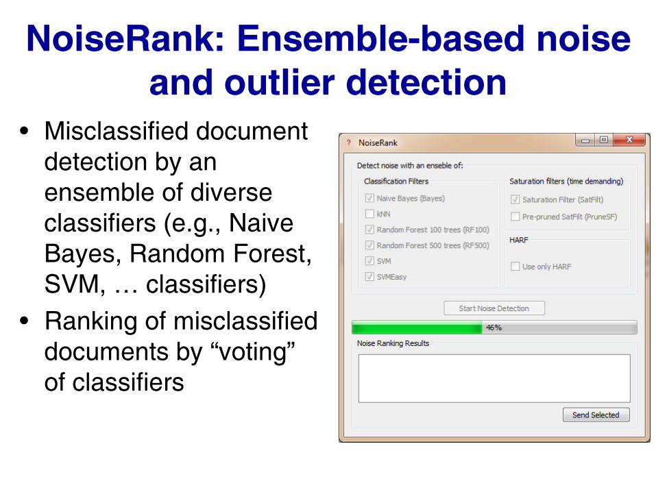
NoiseRank: Ensemble-based noise
and outlier detection
• Misclassified document
detection by an
ensemble of diverse
classifiers (e.g., Naive
Bayes, Random Forest,
SVM, … classifiers)
• Ranking of misclassified
documents by “voting”
of classifiers
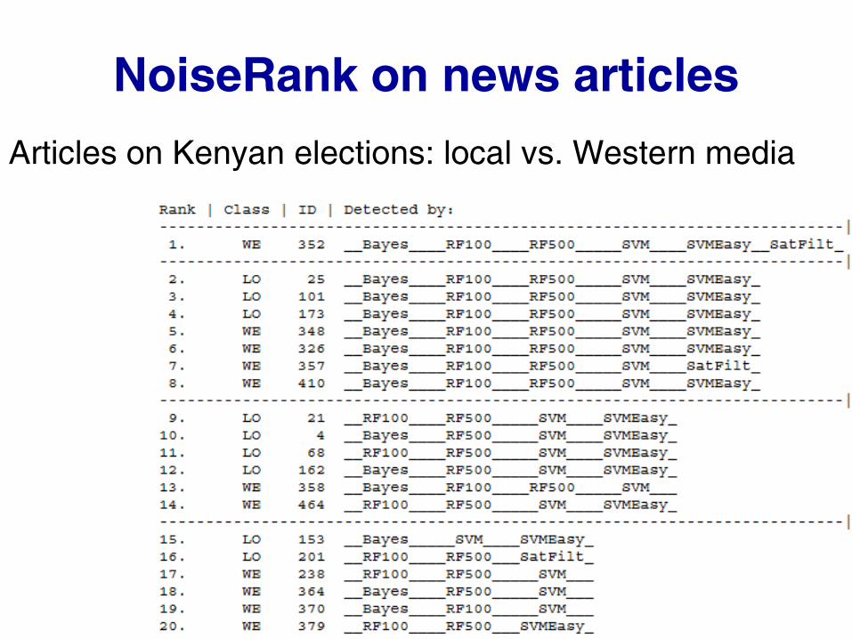
NoiseRank on news articles
Articles on Kenyan elections: local vs. Western media
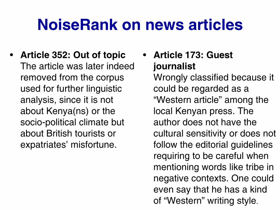
NoiseRank on news articles
• Article 352: Out of topic
The article was later indeed
removed from the corpus
used for further linguistic
analysis, since it is not
about Kenya(ns) or the
socio-political climate but
about British tourists or
expatriates’ misfortune.
• Article 173: Guest
journalist
Wrongly classified because it
could be regarded as a
“Western article” among the
local Kenyan press. The
author does not have the
cultural sensitivity or does not
follow the editorial guidelines
requiring to be careful when
mentioning words like tribe in
negative contexts. One could
even say that he has a kind
of “Western” writing style.
Advanced Topics
• Text mining: An introduction
• Document clustering and outlier
• Wordification approach to relational data mining
330
Motivation
• Develop a RDM technique inspired by text
mining
• Using a large number of simple, easy to
understand features (words)
• Improved scalability, handling large datasets
• Used as a preprocessing step to propositional
learners
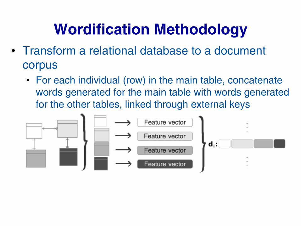
Wordification Methodology
• Transform a relational database to a document
corpus
• For each individual (row) in the main table, concatenate
words generated for the main table with words generated
for the other tables, linked through external keys
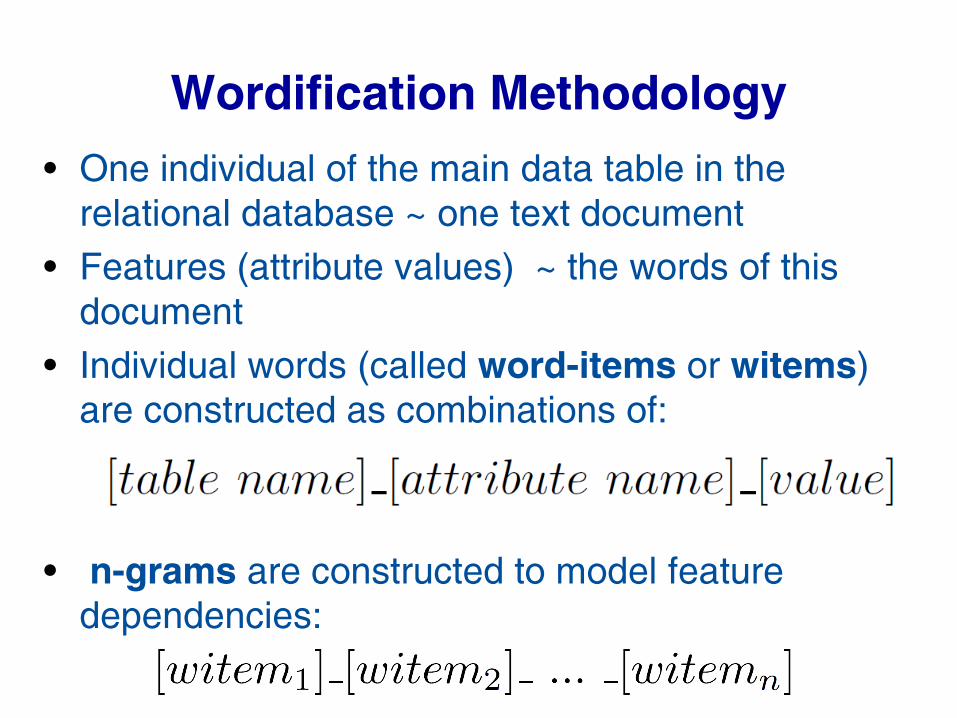
Wordification Methodology
• One individual of the main data table in the
relational database ~ one text document
• Features (attribute values) ~ the words of this
document
• Individual words (called word-items or witems)
are constructed as combinations of:
• n-grams are constructed to model feature
dependencies:
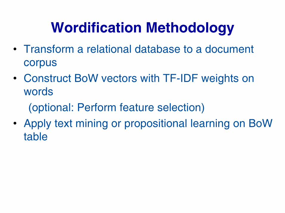
Wordification Methodology
• Transform a relational database to a document
corpus
• Construct BoW vectors with TF-IDF weights on
words
(optional: Perform feature selection)
• Apply text mining or propositional learning on BoW
table
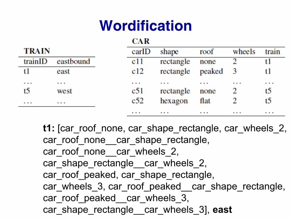
Wordification
t1: [car_roof_none, car_shape_rectangle, car_wheels_2,
car_roof_none__car_shape_rectangle,
car_roof_none__car_wheels_2,
car_shape_rectangle__car_wheels_2,
car_roof_peaked, car_shape_rectangle,
car_wheels_3, car_roof_peaked__car_shape_rectangle,
car_roof_peaked__car_wheels_3,
car_shape_rectangle__car_wheels_3], east
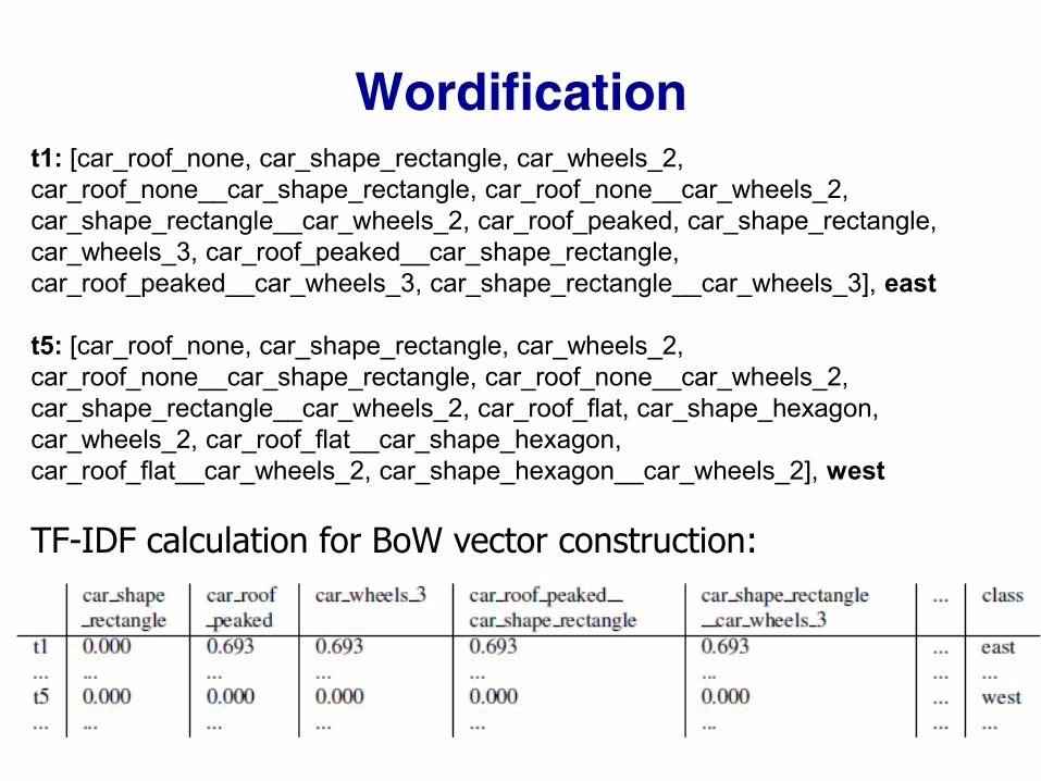
Wordification t1: [car_roof_none, car_shape_rectangle, car_wheels_2,
car_roof_none__car_shape_rectangle, car_roof_none__car_wheels_2,
car_shape_rectangle__car_wheels_2, car_roof_peaked, car_shape_rectangle,
car_wheels_3, car_roof_peaked__car_shape_rectangle,
car_roof_peaked__car_wheels_3, car_shape_rectangle__car_wheels_3], east
t5: [car_roof_none, car_shape_rectangle, car_wheels_2,
car_roof_none__car_shape_rectangle, car_roof_none__car_wheels_2,
car_shape_rectangle__car_wheels_2, car_roof_flat, car_shape_hexagon,
car_wheels_2, car_roof_flat__car_shape_hexagon,
car_roof_flat__car_wheels_2, car_shape_hexagon__car_wheels_2], west
TF-IDF calculation for BoW vector construction:
TF-IDF weights
• No explicit use of existential variables in
features, TF-IDF instead
• The weight of a word indicates how relevant is
the feature for the given individual
• The TF-IDF weights can then be used either for
filtering words with low importance or for using
them directly by a propositional learner (e.g. J48)
Experiments
• Cross-validation experiments on 8 relational
datasets: Trains (in two variants),
Carcinogenesis, Mutagenensis with 42 and 188
examples, IMDB, and Financial.
• Results (using J48 for propositional learning)
Experiments
• Cross-validation experiments on 8 relational
datasets: Trains (in two variants),
Carcinogenesis, Mutagenensis with 42 and 188
examples, IMDB, and Financial.
• Results (using J48 for propositional learning)
– first applying Friedman test to rank the algorithms,
– then post-hoc test Nemenyi test to compare multiple
algorithms to each other
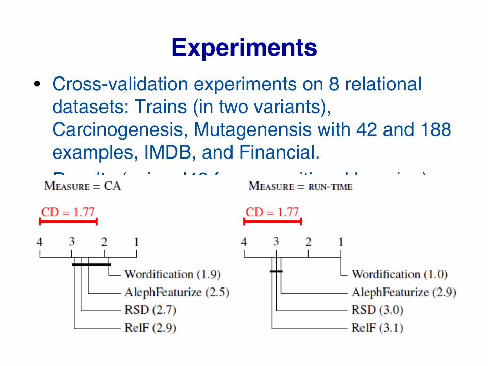
Experiments
• Cross-validation experiments on 8 relational
datasets: Trains (in two variants),
Carcinogenesis, Mutagenensis with 42 and 188
examples, IMDB, and Financial.
• Results (using J48 for propositional learning)
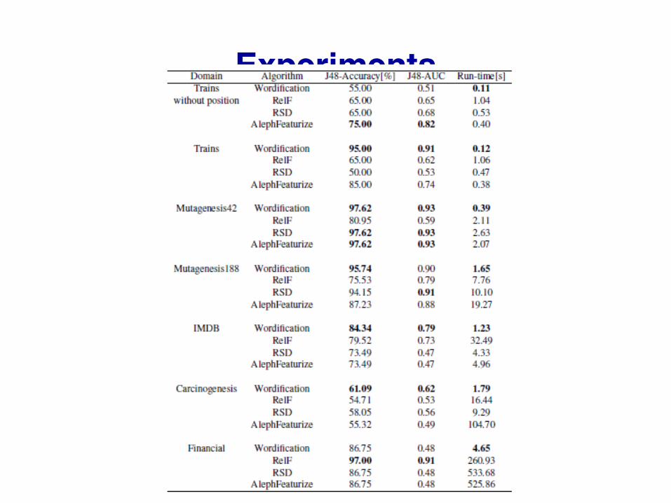
Experiments
Use Case: IMDB
• IMDB subset: Top 250 and bottom 100 movies
• Movies, actors, movie genres, directors, director genres
• Wordification methodology applied
• Association rules learned on BoW vector table
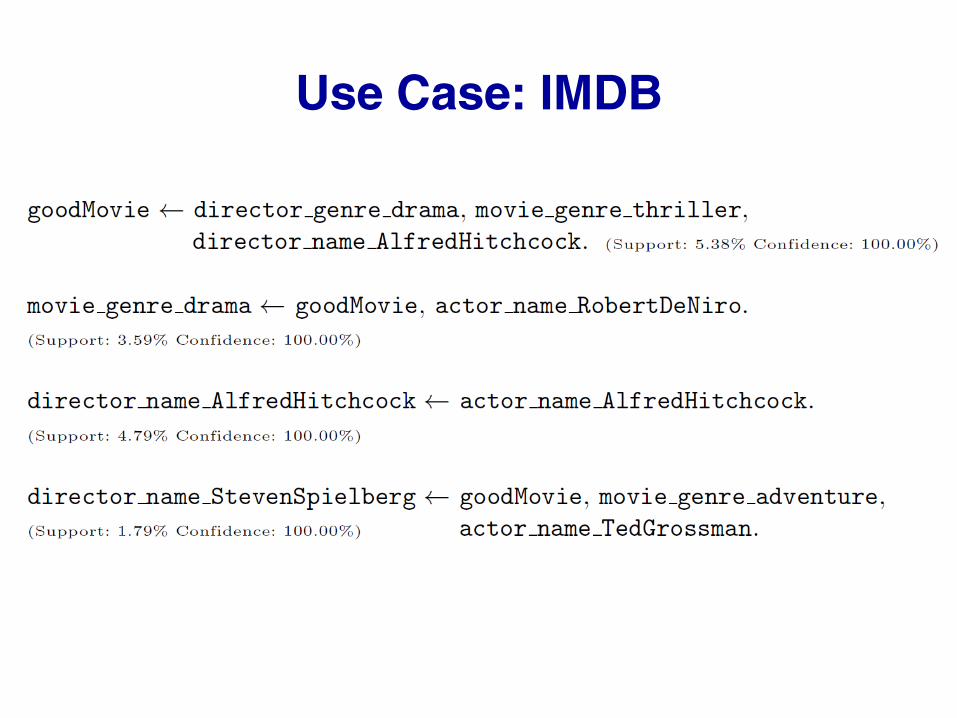
Use Case: IMDB
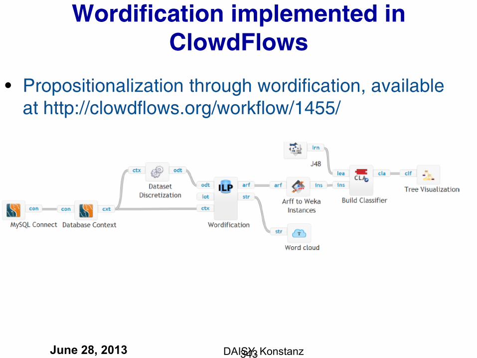
Wordification implemented in
ClowdFlows
June 28, 2013 DAISY, Konstanz 343
• Propositionalization through wordification, available
at http://clowdflows.org/workflow/1455/
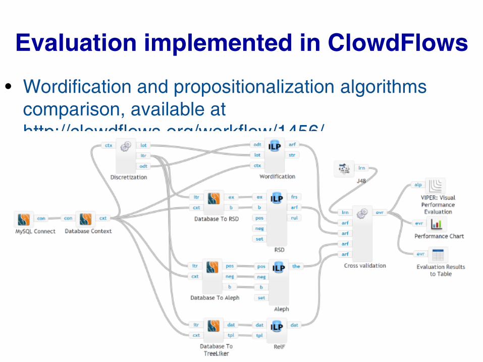
Evaluation implemented in ClowdFlows
June 28, 2013 DAISY, Konstanz 344
• Wordification and propositionalization algorithms
comparison, available at
http://clowdflows.org/workflow/1456/
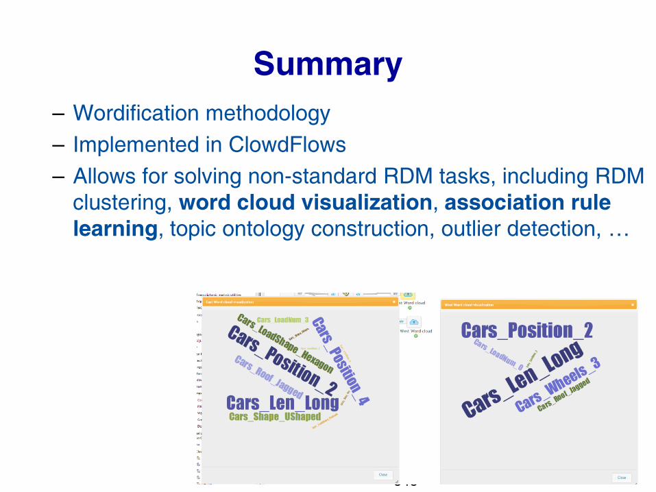
345
Summary
– Wordification methodology
– Implemented in ClowdFlows
– Allows for solving non-standard RDM tasks, including RDM
clustering, word cloud visualization, association rule
learning, topic ontology construction, outlier detection, …