data mining and warehousing -...
TRANSCRIPT
Data mining and Warehousing
| A.Thottarayaswamy M.C.A., M.Phil 1
DATA MINING AND WAREHOUSING

Data mining and Warehousing
| A.Thottarayaswamy M.C.A., M.Phil 2
CONTENTS
UNIT I Introduction 3
Basic data mining tasks – data mining versus knowledge discovery in databases –
data mining issues – data mining metrics – social implications of data mining –
data mining from a database perspective.
Data mining techniques 12
Introduction – a statistical perspective on data mining –similarity measures –
decision trees – neural networks – genetic algorithms.
UNIT II Classification 27
Introduction – Statistical – based algorithms - distance – based algorithms –
decision tree based algorithms - neural network based algorithms –
rule based algorithms – combining techniques.
UNIT III Clustering 51
Introduction – Similarity and Distance Measures – Outliers – Hierarchical Algorithms -
Partitional Algorithms.
Association rules 70
Introduction - large item sets - basic algorithms – parallel & distributed algorithms –
comparing approaches- incremental rules – advanced association rules techniques –
measuring the quality of rules.
UNIT IV Data warehousing 91
Introduction - characteristics of a data warehouse – data marts – other aspects of data mart.
Online analytical processing 95 Introduction - OLTP & OLAP systems – data modelling –star schema for
multidimensional view –data modelling – multifact star schema or snow flake schema
– OLAP TOOLS – State of the market – OLAP TOOLS and the internet.
UNIT V Developing a data warehouse 106
why and how to build a data warehouse –data warehouse architectural strategies and
organization issues - design consideration – data content – metadata distribution of data –
tools for data warehousing – performance considerations – crucial decisions in designing
a data warehouse.
Applications of data warehousing and data mining in government 114
Introduction - national data warehouses – other areas for data warehousing and
data mining.
Reference 117
Appendices - 118
Online Student Resources available at

Data mining and Warehousing
| A.Thottarayaswamy M.C.A., M.Phil 3
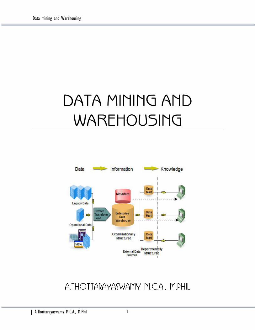
DATA MINING
Data mining is often defined as finding hidden information in a database. Alternatively, it
has been called exploratory data analysis, data driven discovery, and deductive learning.
SQL
Result
Traditional database queries (see above fig), access a database using a well-defined query stated in a
language such as SQL. The output of the query consists of the data from the database that satisfies
the query. Data mining access of a database differs from this traditional access in several ways:
Query: The query might not be well formed or precisely stated. The data miner might not
even be exactly sure of what he wants to see.
Data: The data accessed is usually a different version from that of the original operational
database. The data have been cleansed and modified to better support the mining process.
Output: The output of the data mining query probably is not a subset of the database. Instead
it is the output of some analysis of the contents of the database
The current state of the art of data mining is similar to similar to that of database query
processing in the late 1960s and early 1970s. over the next decade there undoubtedly will be great
strides in extending the state of the art with respect to data mining.
Data mining involves many different algorithms to accomplish different tasks. All of these
algorithms attempt to fit a model to the data. Data mining algorithms can be characterized as
consisting of three parts:
Model: The purpose of the algorithm is to fit a model of the data.
Preference: Some criteria must be used to fit one model over another.
Search: All algorithms require some technique to search the data.
UNIT 1 - Introduction
1.1 Basic data mining tasks
1.2 Data mining versus knowledge discovery in databases
1.3 Data mining issues
1.4 Data mining metrics
1.5 Social implications of data mining
1.6 Data mining from a database perspective.
DBMS DB

Data mining and Warehousing
| A.Thottarayaswamy M.C.A., M.Phil 4
Data mining model
Figure 1 Data mining models and Tasks
A predictive model makes a prediction about values of data using known results found from different
data. Predictive modeling may be made based on the use of other historical data.
A descriptive model identifies patterns or relationships in data. Unlike the predictive model, a
descriptive model server as a way to explore the properties of the data examined, not to predict new
properties. Clustering, summarization, association rules, and sequence discovery are usually viewed
as descriptive in nature.
1.1 BASIC DATA MINING TASKS
1.1.1 Classification:
Classification maps data into predefined groups or classes. It is often referred to as
supervised learning because the classes are determined before examining the data. Classification
algorithms require that the classes be defined based on data attribute values. They often describe
these classes by looking at the characteristics of data already known to belong to the classes.
Pattern recognition is a type of classification where an input pattern is classified into one of several
classes based on its similarity to these predefined classes. Example: An airport security screening station is used to determine if passengers are potential terrorists or
criminals. To do this, the face of each passenger is scanned and its basic pattern is identified.
1.1.2 Regression:
Regression is used to map a data item to real valued prediction variable. In actuality,
regression involves the learning of the function that does this mapping. Regression assumes that the
target data fit into some known type of function (e.g linear, logistic) and then determines the best
function of this type that models the given data. Example:
A college professor wishes to reach a certain level of savings before her retirement. She uses a simple
linear regression formula to predict this value by fitting past behavior.
1.1.3 Time series analysis:
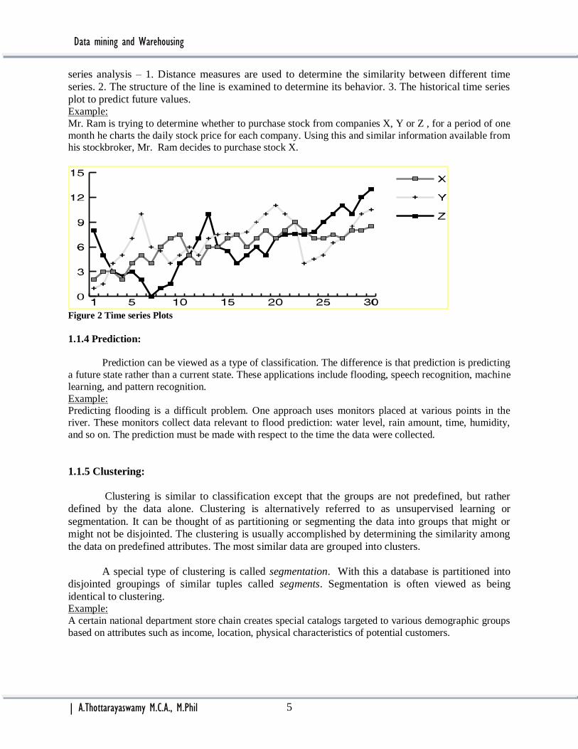
With time series analysis, the value of an attribute is examined as it varies over times. The
values usually are obtained as evenly spaced time points (daily, weekly, hourly etc). a time series plot
(see fig.) is used to visualize the time series, can easily see that the plots for Y and Z have similar
behavior, while X appears to have less volatility. There are three basic functions performed in time
Data mining and Warehousing
| A.Thottarayaswamy M.C.A., M.Phil 5
series analysis – 1. Distance measures are used to determine the similarity between different time
series. 2. The structure of the line is examined to determine its behavior. 3. The historical time series
plot to predict future values. Example:
Mr. Ram is trying to determine whether to purchase stock from companies X, Y or Z , for a period of one
month he charts the daily stock price for each company. Using this and similar information available from his stockbroker, Mr. Ram decides to purchase stock X.
Figure 2 Time series Plots
1.1.4 Prediction:
Prediction can be viewed as a type of classification. The difference is that prediction is predicting
a future state rather than a current state. These applications include flooding, speech recognition, machine
learning, and pattern recognition.
Example: Predicting flooding is a difficult problem. One approach uses monitors placed at various points in the
river. These monitors collect data relevant to flood prediction: water level, rain amount, time, humidity,
and so on. The prediction must be made with respect to the time the data were collected.
1.1.5 Clustering:
Clustering is similar to classification except that the groups are not predefined, but rather
defined by the data alone. Clustering is alternatively referred to as unsupervised learning or
segmentation. It can be thought of as partitioning or segmenting the data into groups that might or
might not be disjointed. The clustering is usually accomplished by determining the similarity among
the data on predefined attributes. The most similar data are grouped into clusters.
A special type of clustering is called segmentation. With this a database is partitioned into
disjointed groupings of similar tuples called segments. Segmentation is often viewed as being
identical to clustering. Example:
A certain national department store chain creates special catalogs targeted to various demographic groups
based on attributes such as income, location, physical characteristics of potential customers.

Data mining and Warehousing
| A.Thottarayaswamy M.C.A., M.Phil 6
1.1.6 Summarization:
Summarization maps data into subsets with associated simple descriptions. Summarization is
also called characterization or generalization.
It extracts or derives representative information about the database. This may be accomplished by
actually retrieving portions of the data. Summary type information can be derived from the data. Example: One of the many criteria used to compare universities by the U.S news & World report is the average
SAT or ACTS score. This is a summarization used to estimate the type and intellectual level of the
student body.
1.1.7 Association rules:
Link analysis, alternatively referred to as affinity analysis or association, refers to the data
mining task of uncovering relationships among data. An association rule is a model that identifies
specific types of data association.
Example:
A grocery store retailer is trying to decide whether to put bread on sale. To help determine
The impact of this decision, the retailer generates association rules that show what other products are
frequently purchased with bread. He finds that 60% of the times that bread is sold so are pretzels and
that 70% of the time jelly is also sold. Based on these facts, he tries to capitalize on the association
between bread, pretzels, and jelly by placing some pretzels and jelly at the end of the aisle where the
bread is placed. In addition, he decides not to place either of these items on sale at the same time.
1.1.8 Sequence discovery:
Sequential analysis or sequence discovery is used to determine sequential patterns in data.
These patterns are based on a time sequence of action. These patterns are similar to association in
that data are found to be related, but the relationship is based on time.
Example:
The Web master at the XYZ Corp. periodically analyzes the Web log data to determine how users of
the XYZ's Web pages access them. He is interested in determining what sequences of pages are
frequently accessed. He determines that 70 percent of the users of page A follow one of the following
patterns of behavior: (A, B, C) or (A, D, B, C) or (A, E, B, C). He then determines to add a link
directly from page A to page C.
1.2 DATA MINING VERSUS KNOWLEDGE DISCOVERY IN DATABASES
The terms knowledge discovery in databases (KDD) and data mining are often used
interchangeably. In fact, there have been. Many other names given to this process of discovering
useful (hidden) patterns in data: knowledge extraction, information discovery, information
harvesting, and unsupervised pattern recognition.
Definition: Knowledge discovery in database (KDD) is the process of finding useful information and
patterns in data.
Definition: Data mining is the use of algorithms to extract the information and patterns derived by
the KDD process.

Data mining and Warehousing
| A.Thottarayaswamy M.C.A., M.Phil 7
The KDD process is often said to be nontrivial; A traditional SQL database query can be
viewed as the data mining part of a KDD process. Indeed, this may be viewed as somewhat simple
and trivial. The definition of KDD includes the keyword useful. Although some definitions have
included the term "potentially useful," we believe that if the information found in the process is not
useful, then it really is not information.
KDD is a process that involves many different steps. The input to this process is the data, and
the output is the useful information desired by the users. The objective may be unclear or inexact.
The process itself is interactive and may require much elapsed time. To ensure the usefulness and
accuracy of the results of the process, interaction throughout the process with both domain experts
and technical experts might be needed.
Figure 3 KDD Process
KDD process consists of the following five steps:
Selection: The data needed for the data mining process may be obtained from many different and
heterogeneous data sources. This first step obtains the data from various databases, files, and non
electronic sources.
Preprocessing: The data to be used by the process may have incorrect or missing data. There may
be anomalous data from multiple sources involving different data types and metrics. There may be
many different activities performed at this time. Erroneous data may be corrected or removed,
whereas missing data must be supplied or predicted (often using data mining tools).
Transformation: Data from different sources must be converted into a common format for
processing. Some data may be encoded or transformed into more usable formats. Data reduction may
be used to reduce the number of possible data values being considered.
Data mining: Based on the data mining task being performed, this step applies algorithms to the
transformed data to generate the desired results.
Interpretation/evaluation: How the data mining results are presented to the users is extremely
important because the usefulness of the results is dependent on it. Various visualization and GUI
strategies are used at this last step.
Visualization refers to the visual presentation of data. The old expression "a picture is worth a
thousand words' certainly is true when examining the structure of data.
Visualization techniques include:
Graphical: Traditional graph structures including bar charts, pie charts, histograms and line
graphs may be used.
Geometric: Geometric techniques include the box plot and scatter diagram techniques.
Icon based: Using figures, colors, or other icons can improve the presentation of the results.
Pixel based: With these techniques each data value is shown as a uniquely colored pixel.
Hierarchical: These techniques hierarchically divide the display area (screen) into regions

Data mining and Warehousing
| A.Thottarayaswamy M.C.A., M.Phil 8
based on data values.
Hybrid: the preceding approaches can be combined into one display.
Any of these approaches may be two-dimensional or three-dimensional. Visualization tools can be
used to summarize data as a data mining technique itself. In addition, visualization can be used to
show the complex results of data mining tasks.
The data mining process itself is complex. As we will see in later chapters, there are many
different data mining applications and algorithms. These algorithms must be carefully applied to be
effective. Discovered patterns must be correctly interpreted and properly evaluated to ensure that the
resulting information is meaningful and accurate.
1.2.1 Development of Data Mining
The current evolution of data mining functions and products is the result of years of influence
from many disciplines, including databases, information retrieval, statistics, algorithms, and machine
learning (see below Fig). Another computer science area that has had a major impact on the KDD
process is multimedia and graphics. A major goal of KDD is to be able to describe the results of the
KDD process in a meaningful manner. Because many different results are often produced, this is a
nontrivial problem. Visualization techniques often involve sophisticated multimedia and graphics
presentations.
Below Table shows developments in the areas of artificial intelligence (AI), information
retrieval (IR), databases (DB), and statistics (Stat) leading to the current view of data mining.
These different historical influences, which have led to the development of the, total data mining
area, have given rise to different views of what data mining functions actually are:
Induction is used to proceed from very specific knowledge to more general information.
This type of technique is often found in AI applications.
Because the primary objective of data mining is to describe some characteristics of a set of
data by a general model, this approach can be viewed as a type of compression. Here the
detailed data within the database are abstracted and compressed to a smaller description of
the data characteristics that are found in the model.
As stated earlier, the data mining process itself can be viewed as a type of querying the
underlying database. Indeed, an ongoing direction of data mining research is how to define
a data mining query and whether a query language (like SQL) can be developed to capture
the many different types of data mining queries.
Describing a large database can be viewed as using approximation to help uncover hidden
information about the data.
When dealing with large databases, the impact of size and efficiency of developing an
abstract model can be thought of as a type of search problem.

Data mining and Warehousing
| A.Thottarayaswamy M.C.A., M.Phil 9
1.3 DATA MINING ISSUES
There are many important implementation issues associated with data mining:
Human interaction: Since data mining problems are often not precisely stated, interfaces
may be needed with both domain and technical experts. Technical experts are used to formulate the
queries and assist in interpreting the results.
Over fitting: When a model is generated that is associated with a given database state, it is
desirable that the model also fit future database states. Over fitting occurs when the model does not
fit future states. This may be caused by assumptions that are made about the data or may simply be
caused by the small size of the training database. For example, a classification model for an
employee database may be developed to classify employees as short, medium, or tall. If the training
database is quite small, the model might erroneously indicate that a short person is anyone fewer than
five feet eight inches because there is only one entry in the training database under five feet eight. In
this case, many future employees would be erroneously classified as short. Over fitting can, arise
under other circumstances as well, even though the data are not changing.
Outliers: There are often many data entries that do not fit nicely into the derived model. This
becomes even more of an issue with very large databases. If a model is developed that includes these
outliers, then the model may not behave well for data that are not outliers.
Interpretation of results: Currently, data mining output may require experts to correctly
interpret the results, which might otherwise be meaningless to the average database user.
Visualization of results: To easily view and understand the output of data mining algorithms,
visualization of the results is helpful.
Large datasets: The massive datasets associated with data mining create problems when
applying algorithms designed for small datasets. Many modeling applications grow exponentially on
the dataset size and thus are too inefficient for larger datasets. Sampling and parallelization are
effective tools to attack this scalability problem.
High dimensionality: A conventional database schema may be composed of many different
attributes. The problem here is that not all attributes may be needed to, solve a given data mining
problem. The use of some attributes may interfere with the correct completion of a data mining task.
The use of other attributes may simply increase the overall complexity and decrease the efficiency of
an algorithm. This problem is sometimes referred to as the dimensionality curse, meaning that there
are many attributes (dimensions) involved and it is difficult to determine which ones should be used.
One solution to this high dimensionality problem is to reduce the number of attributes, which is
known as dimensionality reduction. However, determining which attributes not needed is not always
easy to do.
Multimedia data: Most previous data mining algorithms are targeted to traditional data types
(numeric, character, text, etc.). The use of multimedia data such as is found in GIS databases
complicates or invalidates many proposed algorithms.
Missing data: During the preprocessing phase of KDD, missing data may be replaced with
estimates. This and other approaches to handling missing data can lead to invalid results in the data
mining step.
Irrelevant data: Some attributes in the database might not be of interest to the data mining
task being developed.
Noisy data: Some attribute values might be invalid or incorrect. These values are often
corrected before running data mining applications.
Changing data: Databases cannot be assumed to be static. However, most data mining
algorithms do assume a static database. This requires that the algorithm be completely rerun anytime
the database changes.

Data mining and Warehousing
| A.Thottarayaswamy M.C.A., M.Phil 10
Integration: The KDD process is not currently integrated into normal data processing
activities. KDD requests may be treated as special, unusual, or one-time needs. This makes them
inefficient, ineffective, and not general enough to be used on an ongoing basis. Integration of data
mining functions into traditional DBMS systems is certainly a desirable goal.
Application: Determining the intended use for the information obtained from the data mining
function is a challenge. Indeed, how business executives can effectively use the output is sometimes
considered the more difficult part, not the running of the algorithms themselves. Because the data are
of a type that has not previously been known, business practices may have to be modified to
determine how to effectively use the information uncovered.
1.4 DATA MINING METRICS
Measuring the effectiveness or usefulness of a data mining approach is not always
straightforward. In fact, different metrics could be used for different techniques and also based on the
interest level. From -an overall business or usefulness perspective, a measure such return on
investment (ROI) could be used. ROI examines the difference between what the data mining
technique costs and what the savings or benefits from its use are. Of course, this would be difficult to
measure because the return is hard to quantify. It could be measured as increased sales, reduced
advertising expenditure, or both. In a specific advertising campaign implemented via targeted catalog
mailings, the percentage of catalog recipients and the amount of purchase per recipient would
provide one means to measure the effectiveness of the mailings.
We use a more computer science/database perspective to measure various data mining
approaches. We assume that the business management has determined that a particular data mining
application be made. They subsequently will determine the overall effectiveness of the approach
using some ROI (or related) strategy. Our objective is to compare different alternatives to
implementing a specific data mining task. The metrics used include the traditional metrics of space
and time based on complexity analysis. In some cases, such as accuracy in classification, more
specific metrics targeted to a data mining task may be used.
1.5 SOCIAL IMPLICATIONS OF DATA MINING
The integration of data mining techniques into normal day-to-day activities has become
commonplace. We are confronted daily with targeted advertising, and businesses have become more
efficient through the use of data mining activities to reduce costs. Data mining adversaries, however,
are concerned that this information is being obtained at the cost of reduced privacy. Data mining
applications can derive much demographic information concerning customers that was previously not
known or hidden in the data. The unauthorized use of such data could result in the disclosure of
information that is deemed to be confidential. We have recently seen an increase in interest in data
mining techniques targeted to such applications as fraud detection, identifying criminal suspects, and
prediction of potential terrorists.
These can be viewed as types of classification problems. The approach that is often used here
is one of "profiling" the typical behavior or characteristics involved. Indeed, many classification
techniques work by identifying the attribute values that commonly occur for the target class.
Subsequent records will be then classified based on these attribute values. Keep in mind that these
approaches to classification are imperfect. Mistakes can be made. Just because an individual makes a
series of credit card purchases that are similar to those often made when a card is stolen does not
mean that the card is stolen or that the individual is a criminal.

Data mining and Warehousing
| A.Thottarayaswamy M.C.A., M.Phil 11
Users of data mining techniques must be sensitive to these issues and must not violate any
privacy directives or guidelines.
1.6 DATA MINING FROM A DATABASE PERSPECTIVE
Data mining can be studied from many different perspectives. An IR researcher probably
would concentrate on the use of data mining techniques to access text data; a statistician might
look primarily at the historical techniques, including time series analysis, hypothesis testing, and
applications of Bayes theorem, a machine learning specialist might be interested primarily in data
mining algorithms that learn; and an algorithms researcher would be interested in studying and
comparing algorithms based on type and complexity. The study of data mining from a database
perspective involves looking at all types of data mining applications and techniques. However, we
are interested primarily in those that are of practical interest. While our interest is not limited to
any particular type of algorithm or approach,
we are concerned about the following implementation issues:
Scalability: Algorithms that do not scale up to perform well with massive real world
datasets are of limited application. Related to this is the fact that techniques should work regardless
of the amount of available main memory.
Real-world data: Real-world data are noisy and have many missing attribute values.
Algorithms should be able to work even in the presence of these problems.
Update: Many data mining algorithms work with static datasets. This is not a realistic
assumption.
Ease of use: Although some algorithms may work well, they may not be well received by
users if they are difficult to use or understand.

Data mining and Warehousing
| A.Thottarayaswamy M.C.A., M.Phil 12
1.7 INTRODUCTION
Parametric models describe the relationship between input and output through the use of
algebraic equations where some parameters are not specified. These unspecified parameters are
determined by providing input examples. Even though parametric modeling is a nice theoretical
topic and can sometimes be used, often it is either too simplistic or requires more knowledge
about the data involved than is available. Thus, for real-world problems, these parametric models
may not be useful.
A nonparametric model is one that is data-driven. No explicit equations are used to deter-
mine the model. This means that the modeling process adapts to the data at hand. Unlike
parametric modeling, where a specific model is assumed ahead of time, the nonparametric
techniques create a model based on the input. While the parametric methods require more
knowledge about the data before the modeling process, the nonparametric technique requires a
large amount of data as input to the modeling process itself. The modeling process then creates
the model by sifting through the data. Recent nonparametric methods have employed machine
learning techniques to be able to learn dynamically as data are added to the input. Thus, the more
data, the better the model created. Also, this dynamic learning process allows the model to be
created continuously as the data is input. These features make nonparametric techniques
particularly suitable to database
1.8 STATISTICAL PERSPECTIVE ON DATA MINING
There have been many statistical concepts that are the basis for data mining techniques. We briefly
review some of these concepts.
1.8.1 Point Estimation
Point estimation refers to the process of estimating a population parameter, Θ by an estimate of the
parameter, Θ. This can be done to estimate mean, variance, standard deviation, or any other statistical
parameter. Often the estimate of the parameter for a general population may be made by actually
calculating the parameter value for a population sample. An estimator technique may also be used to
estimate (predict) the value of missing data. The bias of estimator is the difference between the
expected value of the estimator and the actual value:
UNIT 1 – Data Mining Techniques
1.7 Introduction
1.8 A Statistical Perspective on data mining
1.9 Similarity Measures
1.10 Decision Trees
1.11 Neural Networks
1.12 Genetic Algorithms
Data mining and Warehousing
| A.Thottarayaswamy M.C.A., M.Phil 13
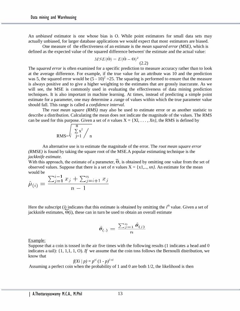
An unbiased estimator is one whose bias is O. While point estimators for small data sets may
actually unbiased, for larger database applications we would expect that most estimators are biased.
One measure of the effectiveness of an estimate is the mean squared error (MSE), which is
defined as the expected value of the squared difference between' the estimate and the actual value:
(2.2)
The squared error is often examined for a specific prediction to measure accuracy rather than to look
at the average difference. For example, if the true value for an attribute was 10 and the prediction
was 5, the squared error would be (5 - 10)2 =25. The squaring is performed to ensure that the measure
is always positive and to give a higher weighting to the estimates that are grossly inaccurate. As we
will see, the MSE is commonly used in evaluating the effectiveness of data mining prediction
techniques. It is also important in machine learning. At times, instead of predicting a simple point
estimate for a parameter, one may determine a .range of values within which the true parameter value
should fall. This range is called a confidence interval.
The root mean square (RMS) may also be used to estimate error or as another statistic to
describe a distribution. Calculating the mean does not indicate the magnitude of the values. The RMS
can be used for this purpose. Given a set of n values X = {Xl, . . . , Xn}, the RMS is defined by
n
∑ x2
RMS=√ j=1 n
An alternative use is to estimate the magnitude of the error. The root mean square error
(RMSE) is found by taking the square root of the MSE.A popular estimating technique is the
jackknife estimate.
With this approach, the estimate of a parameter, Θ, is obtained by omitting one value from the set of
observed values. Suppose that there is a set of n values X = {x1,.., xn}. An estimate for the mean
would be
Here the subscript (i) indicates that this estimate is obtained by omitting the ith value. Given a set of
jackknife estimates, Θ(i), these can in turn be used to obtain an overall estimate
Example:
Suppose that a coin is tossed in the air five times with the following results (1 indicates a head and 0
indicates a tail): {1, 1,1, 1, O). If we assume that the coin toss follows the Bernoulli distribution, we
know that
f(Xi | p) = pxi (1 - p)1-xi
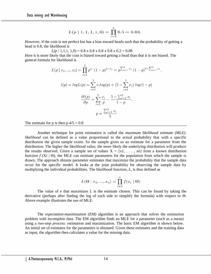
Assuming a perfect coin when the probability of 1 and 0 are both 1/2, the likelihood is then
Data mining and Warehousing
| A.Thottarayaswamy M.C.A., M.Phil 14
However, if the coin is not perfect but has a bias toward heads such that the probability of getting a
head is 0.8, the likelihood is
L(p | 1,1,1, 1,0) = 0.8 x 0.8 x 0.8 x 0.8 x 0.2 = 0.08
Here it is more likely that the coin is biased toward getting a head than that it is not biased. The
general formula for likelihood is
The estimate for p is then p 4/5 = 0.8
Another technique for point estimation is called the maximum likelihood estimate (MLE).
likelihood can be defined as a value proportional to the actual probability that with a specific
distribution the given sample exists. So the sample gives us an estimate for a parameter from the
distribution. The higher the likelihood value, the more likely the underlying distribution will produce
the results observed. Given a sample set of values X = {x1, . . . , xn} from a known distribution
function f (Xi | Θ), the MLE can estimate parameters for the population from which the sample is
drawn. The approach obtains parameter estimates that maximize the probability that the sample data
occur for the specific model. It looks at the joint probability for observing the sample data by
multiplying the individual probabilities. The likelihood function, L, is thus defined as
The value of e that maximizes L is the estimate chosen. This can be found by taking the
derivative (perhaps after finding the log of each side to simplify the formula) with respect to Θ.
Above example illustrates the use of MLE.
The expectation-maximization (EM) algorithm is an approach that solves the estimation
problem with incomplete data. The EM algorithm finds an MLE for a parameter (such as a mean)
using a two-step process: estimation and maximization. The basic EM algorithm is shown below.
An initial set of estimates for the parameters is obtained. Given these estimates and the training data
as input, the algorithm then calculates a value for the missing data.

Data mining and Warehousing
| A.Thottarayaswamy M.C.A., M.Phil 15
EM ALGORITHM :
Example:
1.8.2 Models based on Summarization
There are many basic concepts that provide an abstraction and summarization of the data as a
whole. The basic well-known statistical concepts such as mean, variance, standard deviation,
median, and mode are simple models of the underlying population. Fitting a population to a specific
frequency distribution provides an even better model of the data. Of course, doing this with large
databases that have multiple attributes, have complex and/or multimedia attributes, and are
constantly changing is not practical (let alone always possible).
There are also many well-known techniques to display the structure of the data graphically.
For example, a histogram shows the distribution of the data. A box plot is a more sophisticated

Data mining and Warehousing
| A.Thottarayaswamy M.C.A., M.Phil 16
technique that illustrates several different features of the population at once. Below Figure shows a
sample box plot. The total range of the data values is divided into four equal parts called quartiles.
The box-in the center of the figure shows the range between the first, second, and third quartiles.
The line in the box shows the median. The lines extending from either end of the box are the values
that are a distance of 1.5 of the inter quartile range from the first and third quartiles, respectively.
Outliers are shown as points beyond these values.
Figure 4 Box plot example
Another visual technique to display data is
called a scatter diagram. This is a graph on a two-
dimensional axis of points representing the
relationships between X and y values. By plotting the
actually observable (x, y) points as seen in a sample, a
visual image of some derivable functional relationship
between the x and y values in the total population may
be seen. Below figure shows a scatter diagram that
plots some observed values. Notice that even though
the points do not lie on a precisely linear line, they do
hint that this may be a good predictor of the relationship between x and y.
Fig Scatter diagram example
1.8.3 Bayes theorem
With statistical inference, information about a data distribution are inferred by examining
data that follow that distribution. Given a set of data X = {X1, ..., xn}, a data mining problem is to
uncover properties of the distribution from which the set comes. Bayes rule, defined in Definition
3.1, is a technique to estimate the likelihood of a property given the set of data as evidence or input.
Suppose that either hypothesis h1 or hypothesis h2 must occur, but not both. Also suppose that Xi is
an observable event.
Definition P(h1 | Xi) = P(Xi 1 hl)P(hl)
P(Xi | h1)P(h1) + P(Xi | h2)P(h2)
Here P(h1 | Xi) is called the posterior probability, while P(h1) is the prior probability
associated with hypothesis h1. P (Xi) is the probability of the occurrence of data value Xi and
P(Xi | h1) is the conditional probability that, given a hypothesis, the tuple satisfies it.

Data mining and Warehousing
| A.Thottarayaswamy M.C.A., M.Phil 17
Example:
TABLE 3.1: Training Data for
Example 3.3
Id Income Credit Class xi
1 4 Excellent h1 X4
2 3 Good h1 X7
3 2 Excellent h1 X2
4 3 Good h1 X7
5 4 Good h1 X8
6 2 Excellent h1 X2
7 3 Bad h2 X11
8 2 Bad h2 X10
9 3 Bad h3 X11
10 1 Bad h4 X9
Credit authorizations (hypotheses):
h1=authorize purchase, h2 = authorize after further identification, h3=do not authorize,
h4= do not authorize but contact police
Assign twelve data values for all combinations of credit and income:
From training data: P(h1) = 60%;
P(h2)=20%; P(h3)=10%; P(h4)=10%.
Calculate P(xi | hj) and P(xi)
Ex: P(x7|h1)=2/6; P(x4|h1)=1/6; P(x2|h1)=2/6; P(x8|h1)=1/6; P(xi|h1)=0 for all other xi.
Predict the class for x4:
– Calculate P(hj|x4) for all hj.
– Place x4 in class with largest value.
– Ex:
P(h1|x4)=(P(x4|h1)(P(h1))/P(x4)
=(1/6)(0.6)/0.1=1.
x4 in class h1.
1 2 3 4
Excellent x1 x2 x3 x4
Good x5 x6 x7 x8
Bad x9 x10 x11 x12

Data mining and Warehousing
| A.Thottarayaswamy M.C.A., M.Phil 18
1.8.4 Hypothesis testing
Hypothesis testing attempts to find a model that explains the observed data by first creating a
hypothesis and then testing the hypothesis against the data. This is contrast to most data mining
approaches, which create the model from the actual data without guessing what it is first. The actual
data itself drive the model creation. The hypothesis usually is verified by examining a data sample. If
the hypothesis holds for the sample, it is assumed to hold for the population in general. Given a
population, the initial (assumed) hypothesis to be tested, H0 is called the null hypothesis. Rejection of
the null hypothesis causes another hypothesis, H1, called the alternative hypothesis, to be made.
One technique to perform hypothesis testing is based on the use of the chi-squared statistic.
Actually, there is a set of procedures referred to as chi squared. These procedures can be used to test
the association between two observed variable values and to determine if a set of observed variable
values is statistically significant (i.e., if it differs from the expected case). A hypothesis is first made,
and then the observed values are compared based on this hypothesis. Assuming that 0 represents the
observed data and E is the expected values based on the hypothesis, the chi-squared statistic, X2, is
defined as:
When comparing a set of observed variable values to determine statistical significance, the
values are compared to those of the expected case. This may be the uniform distribution.
Example:
Suppose that there are five schools being compared based on students' results on a set of standardized
achievement tests. The school district expects that the results will be the same for each school. They
know that the total score for the schools is 375, so the expected result would be that each school has
an average score of 75. The actual average scores from the schools are: 50,93,67,78, and 87. The
district administrators want to determine if this is statistically significant. Or in simpler terms, should
they be worried about the distribution of scores. The chi-squared measure here is
X2 = (50-75)2 + (93-75)2 + (67-75)2 + (78-75)2 + (87-75)2 = 15.55
75 75 75 75 75
Examining a chi-squared significance table, it is found that this value is significant. With a degree of
freedom of 4 and a significance level of 95%, the critical value is 9.488. Thus, the administrators
observe that the variance between the schools' scores and the expected values cannot be associated
with pure chance.
1.8.5 Regression and Correlation
Both bivariate regression and correlation can be used to evaluate the strength of a relationship
between two variables. Regression is generally used to predict future values based on past values by
fitting a set of points to a curve. Correlation, however, is used to examine the degree to which the
values for two variables behave similarly.
Linear regression assumes that a linear relationship exists between the input data and the
output data. The common formula for a linear relationship is used in this model:
y = c0 + c1 x1 + … + cn xn
Data mining and Warehousing
| A.Thottarayaswamy M.C.A., M.Phil 19
Here there are n input variables, which are called predictors or regressors; one output variable (the
variable being predicted), which is called the response; and n + 1 constants, which are chosen during
the modeling process to match the input examples (or sample). This is sometimes called multiple
linear regressions because there is more than one predictor.
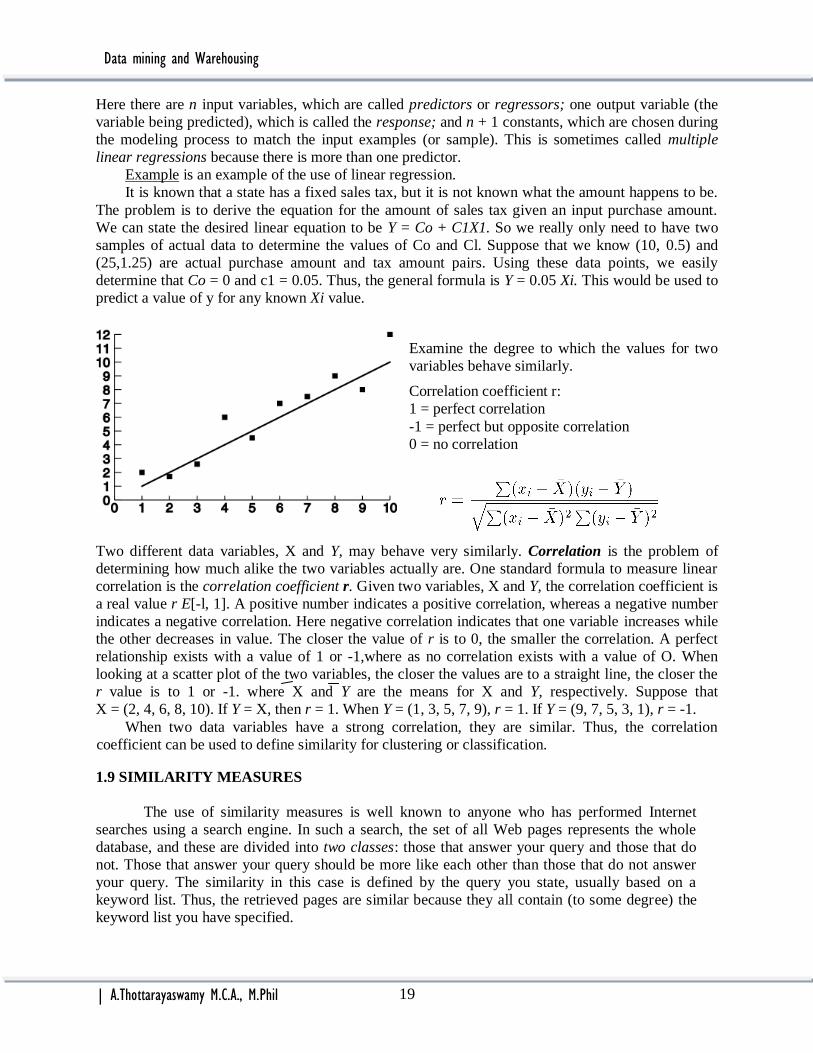
Example is an example of the use of linear regression.
It is known that a state has a fixed sales tax, but it is not known what the amount happens to be.
The problem is to derive the equation for the amount of sales tax given an input purchase amount.
We can state the desired linear equation to be Y = Co + C1X1. So we really only need to have two
samples of actual data to determine the values of Co and Cl. Suppose that we know (10, 0.5) and
(25,1.25) are actual purchase amount and tax amount pairs. Using these data points, we easily
determine that Co = 0 and c1 = 0.05. Thus, the general formula is Y = 0.05 Xi. This would be used to
predict a value of y for any known Xi value.
Examine the degree to which the values for two
variables behave similarly.
Correlation coefficient r:
1 = perfect correlation
-1 = perfect but opposite correlation
0 = no correlation
Two different data variables, X and Y, may behave very similarly. Correlation is the problem of
determining how much alike the two variables actually are. One standard formula to measure linear
correlation is the correlation coefficient r. Given two variables, X and Y, the correlation coefficient is
a real value r E[-l, 1]. A positive number indicates a positive correlation, whereas a negative number
indicates a negative correlation. Here negative correlation indicates that one variable increases while
the other decreases in value. The closer the value of r is to 0, the smaller the correlation. A perfect
relationship exists with a value of 1 or -1,where as no correlation exists with a value of O. When
looking at a scatter plot of the two variables, the closer the values are to a straight line, the closer the
r value is to 1 or -1. where X and Y are the means for X and Y, respectively. Suppose that
X = (2, 4, 6, 8, 10). If Y = X, then r = 1. When Y = (1, 3, 5, 7, 9), r = 1. If Y = (9, 7, 5, 3, 1), r = -1.
When two data variables have a strong correlation, they are similar. Thus, the correlation
coefficient can be used to define similarity for clustering or classification.
1.9 SIMILARITY MEASURES
The use of similarity measures is well known to anyone who has performed Internet
searches using a search engine. In such a search, the set of all Web pages represents the whole
database, and these are divided into two classes: those that answer your query and those that do
not. Those that answer your query should be more like each other than those that do not answer
your query. The similarity in this case is defined by the query you state, usually based on a
keyword list. Thus, the retrieved pages are similar because they all contain (to some degree) the
keyword list you have specified.

Data mining and Warehousing
| A.Thottarayaswamy M.C.A., M.Phil 20
The idea of similarity measures can be abstracted and applied to more general
classification problems. The difficulty lies in how the similarity measures are defined and applied
to the items in the database. Since most similarity measures assume numeric (and often discrete)
values, they may be difficult to use for more general data types. A mapping from the attribute
domain to a subset of the integers may be used.
Definition: The similarity between two tuples ti and tj, sim(ti, tj), in a database D is a mapping from
DxD to the range [0, 1]. Thus sim(ti, tj) [0, 1].
The objective is to define the similarity mapping such that documents that are more alike have a
higher similarity value. Thus, the following are desirable characteristics of a good similarity measure:
This makes the problem an O(n) problem rather than an O(n2) problem. Here are some of
the more common similarity measures used in traditional IR systems and more recently in Internet
search engines:
Distance or dissimilarity measures are often used instead of similarity measures) as implied.
These measure how "unlike" items are. Traditional distance measures may be used in a two-
dimensional space. These include
1.10 DECISION TREES
A decision tree is a predictive modeling technique used in classification, clustering, and
prediction tasks. Decision trees use a "divide and conquer" technique to split the problem search
space into subsets. It is based on the "Twenty Questions" game that children play, as illustrated by
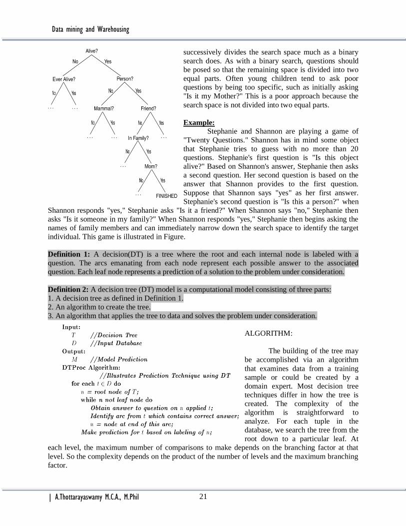
Example and below Figure, graphically shows the steps in the game. This tree has as the root the first
question asked. Each subsequent level in the tree consists of questions at that stage in the game.
Nodes at the third level show questions asked at the third level in the game. Leaf nodes represent a
successful guess as to the object being predicted. This represents a correct prediction. Each question
Data mining and Warehousing
| A.Thottarayaswamy M.C.A., M.Phil 21
successively divides the search space much as a binary
search does. As with a binary search, questions should
be posed so that the remaining space is divided into two
equal parts. Often young children tend to ask poor
questions by being too specific, such as initially asking
"Is it my Mother?" This is a poor approach because the
search space is not divided into two equal parts.
Example:
Stephanie and Shannon are playing a game of
"Twenty Questions." Shannon has in mind some object
that Stephanie tries to guess with no more than 20
questions. Stephanie's first question is "Is this object
alive?" Based on Shannon's answer, Stephanie then asks
a second question. Her second question is based on the
answer that Shannon provides to the first question.
Suppose that Shannon says "yes" as her first answer.
Stephanie's second question is "Is this a person?" when
Shannon responds "yes," Stephanie asks "Is it a friend?" When Shannon says "no," Stephanie then
asks "Is it someone in my family?" When Shannon responds "yes," Stephanie then begins asking the
names of family members and can immediately narrow down the search space to identify the target
individual. This game is illustrated in Figure.
Definition 1: A decision(DT) is a tree where the root and each internal node is labeled with a
question. The arcs emanating from each node represent each possible answer to the associated
question. Each leaf node represents a prediction of a solution to the problem under consideration.
Definition 2: A decision tree (DT) model is a computational model consisting of three parts:
1. A decision tree as defined in Definition 1.
2. An algorithm to create the tree.
3. An algorithm that applies the tree to data and solves the problem under consideration.
ALGORITHM:
The building of the tree may
be accomplished via an algorithm
that examines data from a training
sample or could be created by a
domain expert. Most decision tree
techniques differ in how the tree is
created. The complexity of the
algorithm is straightforward to
analyze. For each tuple in the
database, we search the tree from the
root down to a particular leaf. At
each level, the maximum number of comparisons to make depends on the branching factor at that
level. So the complexity depends on the product of the number of levels and the maximum branching
factor.

Data mining and Warehousing
| A.Thottarayaswamy M.C.A., M.Phil 22
Example:
Suppose that students in a particular university
are to be classified as short, tall, or medium based on
their height. Assume that the database schema is {name,
address, gender, height, age, year, major}. To construct a
decision tree, we must identify the attributes that are
important to the classification problem at hand. Suppose
that height, age, and gender are chosen. Certainly, a
female who is 1.95 m in height is considered as tall, while a male of the same height may not be
considered tall. Also, a child 10 years of age may be tall if he or she is only -1.5 m. Since this is a set
of university students, we would expect most of them to be over 17 years of age. We thus decide to
filter out those under this age and perform their classification separately.
We may consider these students to be outliers because their ages (and more important their
height classifications) are not typical of most university students. Thus, for classification we have
only gender and height. Using these two attributes, a decision tree building algorithm will construct a
tree using a sample of the database with known classification values. This training sample forms the
basis of how the tree is constructed. One possible resulting tree after training is shown in Figure
linear regression.
1.11 Neural networks:
The first proposal to use an artificial neuron appeared in 1943, but computer usage of
neural networks did not actually begin until the 1980s. Neural networks (NN), often referred to as
artificial neural networks (ANN) distinguish them from biological neural networks, are modeled
after the workings of the human brain. The NN is actually an information processing system that
consists of a graph representing the processing system as well as various algorithms that access that
graph.
As with the human brain, the NNs consists of many connected processing elements.
The NN, then, is structured as a directed graph with many nodes (processing elements) and arcs
(interconnections) between them. The nodes in the graph are like individual neurons, while the arcs
are their interconnections. Each of these processing elements functions independently from the
others and uses only local data (input and output to the node) to direct its processing. This feature
facilitates the use of NNs in a distributed and/or parallel environment.
The NN approach, like decision trees, requires that a graphical structure be built to
represent the model and then that the structure be applied to the data. The NN can be viewed as a
directed graph with source (input), sink (output), and internal (hidden) nodes input nodes exist in a
input layer, while the output nodes exist in an output layer. The hidden nodes exist over one or
more hidden layers).
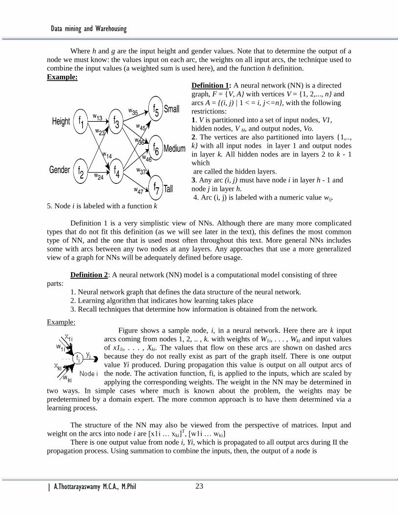
we assume that there is one hidden layer and thus a total of three layers in the general
structure. We arbitrarily assume that there are two nodes in this hidden layer. Each node is labeled
with a function that indicates its effect on the data coming into that node. At the input layer,
functions f1 and f2 simply take the corresponding attribute value in and replicate it as output on each
of the arcs coming out of the node. The functions at the hidden layer, f3 and f4, and those at the
output layer, f5, f6, and f7, perform more complicated functions, which are investigated later in this
section. The arcs are all labeled with weights, where Wij is the weight between nodes i and j. During
processing, the functions at each node are applied to the input data to produce the output. For
example, the output of node 3 is f3(w13h+w23g).
Data mining and Warehousing
| A.Thottarayaswamy M.C.A., M.Phil 23
Where h and g are the input height and gender values. Note that to determine the output of a
node we must know: the values input on each arc, the weights on all input arcs, the technique used to
combine the input values (a weighted sum is used here), and the function h definition.
Example:
Definition 1: A neural network (NN) is a directed
graph, F = {V, A} with vertices V = {1, 2,..., n} and
arcs A = {(i, j) | 1 < = i, j<=n}, with the following
restrictions:
1. V is partitioned into a set of input nodes, V1,
hidden nodes, V H, and output nodes, Vo.
2. The vertices are also partitioned into layers {1,..,
k} with all input nodes in layer 1 and output nodes
in layer k. All hidden nodes are in layers 2 to k - 1
which
are called the hidden layers.
3. Any arc (i, j) must have node i in layer h - 1 and
node j in layer h.
4. Arc (i, j) is labeled with a numeric value wij.
5. Node i is labeled with a function k
Definition 1 is a very simplistic view of NNs. Although there are many more complicated
types that do not fit this definition (as we will see later in the text), this defines the most common
type of NN, and the one that is used most often throughout this text. More general NNs includes
some with arcs between any two nodes at any layers. Any approaches that use a more generalized
view of a graph for NNs will be adequately defined before usage.
Definition 2: A neural network (NN) model is a computational model consisting of three
parts:
1. Neural network graph that defines the data structure of the neural network.
2. Learning algorithm that indicates how learning takes place
3. Recall techniques that determine how information is obtained from the network.
Example: Figure shows a sample node, i, in a neural network. Here there are k input
arcs coming from nodes 1, 2, .. , k. with weights of W1i, . . . , Wki and input values
of x1li, . . . , Xki. The values that flow on these arcs are shown on dashed arcs
because they do not really exist as part of the graph itself. There is one output
value Yi produced. During propagation this value is output on all output arcs of
the node. The activation function, fi, is applied to the inputs, which are scaled by
applying the corresponding weights. The weight in the NN may be determined in
two ways. In simple cases where much is known about the problem, the weights may be
predetermined by a domain expert. The more common approach is to have them determined via a
learning process.
The structure of the NN may also be viewed from the perspective of matrices. Input and
weight on the arcs into node i are [x1i … xki]T, [w1i … wki]
There is one output value from node i, Yi, which is propagated to all output arcs during II the
propagation process. Using summation to combine the inputs, then, the output of a node is

Data mining and Warehousing
| A.Thottarayaswamy M.C.A., M.Phil 24
Here Fi is the activation function. Because NNs are complicated, domain experts and data mining
experts are often advised to assist in their use. This in turn complicates the process.
1.11.1 Activation Function:
The output of each node i in the NN is based on the definition of a function Ii, activation
function, associated with it. An activation function is sometimes called a processing element function
or a squashing function. The function is applied to the set of inputs coming in on the input arcs.
Figure definition example illustrates the process. There have been many proposals for activation
functions, including threshold, sigmoid,
symmetric sigmoid, and Gaussian.
An activation function may also be
called a firing rule, relating it back to the
workings of the human brain. When the input
to a neuron is large enough, it fires, sending an
electrical signal out on its axon (output link).
Likewise, in an artificial NN the output may
be generated only if the input is above a
certain level; thus, the idea of a firing rules. When dealing only with binary output, the output is
either 0 or 1, depending on whether the neuron should fire. Some activation functions use -1 and 1
instead, while still others output a range of values. Based on these ideas, the input and output values
are often considered to be either 0 or 1. The model used in this text is more general, allowing any
numeric values for weights and input/output values. In addition, the functions associated with each
node may be more complicated than a simple threshold function. Since many learning algorithms
use the derivative of the activation function, in these cases the function should have a derivative that
is easy to find.
An activation function, fi, is applied to the input values {X1i, . . . , Xki} and weights
{W1i,..., Wki}. These inputs are usually
combined in a sum of products form S =
(∑kh=1 (Whi Xhi)). If a bias input exists, this
formula becomes S = Woi +(∑kh=1 (Whi
Xhi)). The following are alternative
definitions for activation functions, fi (S) at
node I, activation functions may be
unipolar, with values in [0, 1], or bipolar,
with values in [-1, 1]. The functions are
also shown in above threshold, sigmoid,
Gaussian Figure.
Data mining and Warehousing
| A.Thottarayaswamy M.C.A., M.Phil 25
1.12 GENETIC ALGORITHMS
Genetic algorithms are examples of evolutionary computing methods and are optimization-
type algorithms. Given a population of potential problem solutions (individuals), evolutionary
computing expands this population with new and potentially better solutions. The basis for
evolutionary computing algorithms is biological evolution, where over time evolution produces the
best or "fittest" individuals. Chromosomes, which are DNA strings, provide the abstract model for a
living organism. Subsections of the chromosomes, which are called genes, are used to define
different traits of the individual. During reproduction, genes from the parents are combined to
produce the genes for the child.
In data mining, genetic algorithms may be used for clustering, prediction, and even
association rules. You can think of these techniques as finding the "fittest" models from a set of
models to represent the data. In this approach a starting model is assumed and through much
iteration, models are combined to create new models. The best of these, as defined by a fitness
function, are then input into the next iteration. Algorithms differ in how the model is represented,
how different individuals in the model are combined, and how the fitness function is used.
When using genetic algorithms to solve a problem, the first thing, and perhaps the most
difficult task, that must be determined is how to model the problem as a set of individuals. In the real
world, individuals may be identified by a complete encoding of the DNA structure. An individual
typically is viewed as an array or tuple of values. Based on the recombination (crossover) algorithms,
the values are usually numeric and may be binary strings. These individuals are like a DNA encoding
in that the structure for each individual represents an encoding of the major features needed to model
the problem. Each individual in the population is represented as a string of characters from the given
alphabet.
Definition: Given an alphabet A, an individual or chromosome is a string I = I1, I2, …, In .
where Ij A. each character in the string, Ij, is called a gene. The values that each character can have
are the alleles. A population, P, is a set of individuals.
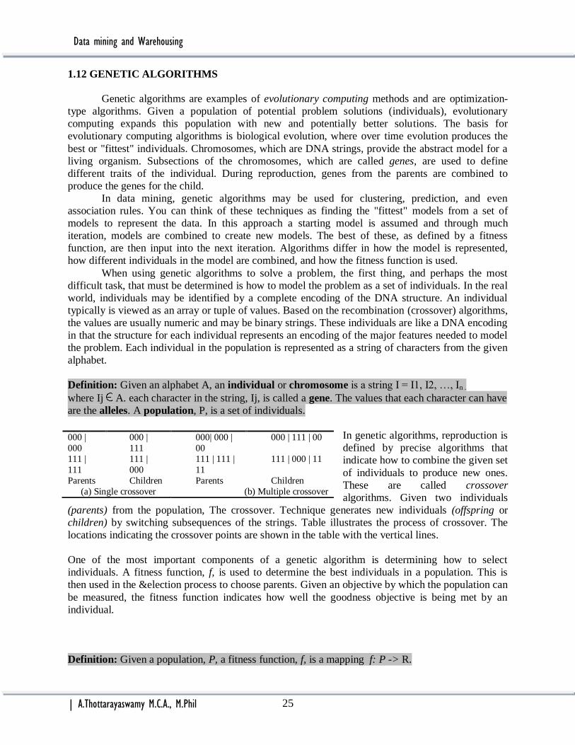
In genetic algorithms, reproduction is
defined by precise algorithms that
indicate how to combine the given set
of individuals to produce new ones.
These are called crossover
algorithms. Given two individuals
(parents) from the population, The crossover. Technique generates new individuals (offspring or
children) by switching subsequences of the strings. Table illustrates the process of crossover. The
locations indicating the crossover points are shown in the table with the vertical lines.
One of the most important components of a genetic algorithm is determining how to select
individuals. A fitness function, f, is used to determine the best individuals in a population. This is
then used in the &election process to choose parents. Given an objective by which the population can
be measured, the fitness function indicates how well the goodness objective is being met by an
individual.
Definition: Given a population, P, a fitness function, f, is a mapping f: P -> R.
000 |
000
000 |
111
000| 000 |
00
000 | 111 | 00
111 |
111
111 |
000
111 | 111 |
11
111 | 000 | 11
Parents Children Parents Children
(a) Single crossover (b) Multiple crossover

Data mining and Warehousing
| A.Thottarayaswamy M.C.A., M.Phil 26
The simplest selection process is to select individuals based on their fitness:
PIi = f(Ii) where ∑ = Ij
∑f(Ij)
Here P Ij is the probability of selecting individual Ii. This type of selection is called roulette wheel
selection. One problem with this approach is that it is still possible to select individuals with a very
low fitness value. In addition, when the distribution is quite skewed with a small number of
extremely fit individuals, these individuals may be chosen repeatedly. In addition, as the search
continues, the population becomes less diverse so that the selection process has little effect.
Definition: A genetic algorithm (GA) is a computational model consisting of five parts:
1. Starting set of individuals, P.
2. Crossover technique.
3. Mutation algorithm.
4. Fitness function.
5. Algorithm that applies the crossover and mutation techniques to P iteratively using the fitness
function to determine the best individuals in P to keep. The algorithm replaces a predefined
number of individuals from the population with each iteration and terminates when some
threshold is met.
ALGORITHM
Algorithm outlines the steps performed
by a genetic algorithm. Initially, a population
of individuals, P, is created. Although
different approaches can be used to perform
this step, they typically are generated
randomly. From this population, a new
population, p’, of the same size is created. The
algorithm repeatedly selects individuals from
whom to create new ones. These parents, i1,
i2, are then used to produce two offspring, o1,
o2, using a crossover process. Then mutants
may be generated. The process continues until
the new population satisfies the termination
condition.
We assume here that the entire
population is replaced with each iteration. An
alternative would be to replace the two
individuals with the smallest fitness. Although
this algorithm is quite general, it is representative of all genetic algorithms. There are many
variations on this general theme. Genetic algorithms have been used to solve most data mining
problems, including classification, clustering, and generating association rules. Typical applications
of genetic algorithms include scheduling, robotics, economics, biology, and pattern recognition.

Data mining and Warehousing
| A.Thottarayaswamy M.C.A., M.Phil 27
2.1 INTRODUCTION
Classification is perhaps the most familiar and most popular data mining technique.
Examples of classification applications include image and pattern recognition, medical diagnosis,
loan approval, detecting faults in industry applications, and classifying financial market trends.
Estimation and prediction may be viewed as types of classification When someone estimates your
age or guesses the number of marbles in a jar, these actually classification problems. Prediction can
be thought of as classifying an attribute value into one of a set of possible classes. It is often viewed
as forecasting a continuous value, while classification forecasts a discrete value. Classification was
frequently performed by simply applying knowledge of the data. This is illustrated in this Example.
Example:
Teachers classify students as A, B, C, D, or F based on their grades. By
using simple boundaries (60, 70, 80, 90) the following classification is
possible.
All approaches to performing classification assume some
knowledge of the data. Often a training set is used to develop the specific
parameters required by the technique. Training data consist of sample
input data as well as the classification assignment for the data. Domain experts may also be used to
assist in the process.
Definition: Given a database D = {t1, t2, … , tn} of tuples (items, records) and a set of classes C=
{C1, … , Cm}, the classification problem is to define a mapping f : D -> C where each ti is assigned
to one class. A class, Cj, contains precisely those tuples mapped to it; that is, Cj = {ti | f(ti) = Cj,
1 <= I <= n, and ti D}
Our definition views classification as a mapping from the database to the set of classes. Note
that the classes are predefined, are non overlapping. And partition the entire database. Each tuple in
the database IS assigned to exactly one class. The classes that exist for a classification problem are
indeed equivalence classes. In actuality, the problem usually is implemented in two phases:
1. Create a specific model by evaluating the training data. This step has as input the training
data and as output a definition of the model developed. The model created classifies the training data
as accurately as possible.
2. Apply the model developed in step 1 by classifying tuples from the target database.
Although the second step actually does the classification (according to the definition in
Definition), most research has been applied to step 1. Step 2 is often straight forward.
UNIT 2 – Classification
2.1 Introduction
2.2 Statistical based algorithms
2.3 Distance based algorithms
2.4 Decision tree based algorithms
2.5 Neural network based algorithms
2.6 Rule based algorithms
2.7 combining techniques
90 < = grade A
80 < = grade < 90 B
70 < = grade < 80 C
60 < = grade < 70 D
grade < 60 F

Data mining and Warehousing
| A.Thottarayaswamy M.C.A., M.Phil 28
There are three basic methods used to solve the classification problem:
1. Specifying boundaries: Here classification is performed by dividing the input space of
potential database tuples into regions where each region is associated with one class.
2. Using probability distributions: For any given class, Cj, P(tj | Cj) is the PDF for the class
evaluated at one point, ti. If a probability of occurrence for each class, P(Cj) is known
(perhaps determined by a domain expert), then P(Cj)P(ti | Cj) is used to estimate the
probability that ti is in class C j .
3. Using posterior probabilities: Given a data value ti, we would like to determine the
probability that ti is in a class Cj. This is denoted by P (Cj | tj) and is called the posterior
probability. One classification approach would be to determine the posterior probability for
each class and then assign ti to the class with the highest probability.
Example:
Suppose we are given that a database consists of tuples of
the form t = (x, y) where 0< = x < = 8 and 0 < = y < = 10.
Figure illustrates the classification problem. Figure (a) shows the
predefined classes by dividing the reference space, Figure (b)
provides sample input data, and Figure (c) shows the
classification of the data based on the defined classes.
A major issue associated with classification is that of over
fitting. If the classification strategy fits the training data exactly,
it may not be applicable to a broader population of data. For
example, suppose that the training data has erroneous or noisy
data. Certainly in this case, fitting the data exactly is not desired.
In the following sections, various approaches to performing
classification are examined. Following table contains data to be
used throughout this chapter to illustrate the various techniques.
This example assumes that the problem is to classify adults as
short, medium, or tall. Table lists height in meters. The last two
columns of this table show two classifications that could be
made, labeled Output1 and Output2, respectively. The Output1
classification uses the simple divisions shown below:
2m < = Height Tall
1.7m < = Height < 2m Medium
Height < = 1.7m Short
Classification algorithm categorization
Statistical Distance DT NN Rules

Data mining and Warehousing
| A.Thottarayaswamy M.C.A., M.Phil 29
2.1.1 Issues in classification:
Missing data: Missing data values
cause problems during both the training
phase and the classification process itself.
Missing values in the training data must be
handled and may produce an inaccurate
result. Missing data in a tuple to be
classified must be able to be handled by the
resulting classification scheme.
There are many approaches to handling
missing data:
Ignore the missing data.
Assume a value for the missing
data. This may be determined by
using some method to predict what
the value could be.
Assume a special value for the
missing data. This means that the
value of missing data is taken to be a specific
value all of its own. Notice the similarity
between missing data in the classification
problem and that of nulls in traditional
databases.
Measuring Performance: Table shows two different classification results using two different
classification tools. Determining which is best depends on the interpretation of the problem by users.
The performance of classification algorithms is usually examined by evaluating the accuracy of the
classification. However, since classification is often a fuzzy problem, the correct answer may depend
on the user. Traditional algorithm evaluation approaches such as determining the space and time
overhead can be used, but these approaches are usually secondary.
Classification accuracy is usually calculated by determining the percentage of tuples placed
in the correct class. This ignores the fact that there also may be a cost associated with an incorrect
assignment to the wrong class. This perhaps should also be determined.
We can examine the performance of classification much as is done with information retrieval
systems. With only two classes, there are four possible outcomes with the classification, as is shown
in below Figure. The upper left and lower right quadrants [for both Figure (a) and (b)] represent
correct actions. The remaining two quadrants are incorrect actions. The performance of a
classification could be determined by associating costs with each of the quadrants. However, this
would be difficult because the total number of costs needed is m2, where m is the number of classes.
Given a specific class, C j, and a database tuple, ti, that tuple may or may not be assigned to
that class while its actual membership mayor may not be in that class. This again gives us the four
quadrants shown in Figure (c), which can be described in the following ways:
True positive (TP): ti predicated to be in Cj and is actually in it.
False positive (FP): ti predicated to be in Cj and is not actually in it.
True negative (TN): ti predicated to be in Cj and is not actually in it.
False negative (FN): ti predicated to be in Cj and is actually in it.
TABLE 1 : Data for Height Classification
Name Gender Height Output1 Output2
Kristina F 1.6 m Short Medium
Jim M 2m Tall Medium
Maggie F 1.9 m Medium Tall
Martha F 1.88 m Medium Tall Stephanie F l.7m Short Medium
Bob M 1.85 m Medium Medium
Kathy F 1.6 m Short Medium
Dave M l.7m Short Medium Worth M 2.2m Tall Tall
Steven M 2.1 m Tall Tall
Debbie F 1.8 m Medium Medium
Todd M 1.95 m Medium Medium
Kim F 1.9 m Medium Tall
Amy F 1.8 m Medium Medium
Wynett F 1.75 m Medium Medium

Data mining and Warehousing
| A.Thottarayaswamy M.C.A., M.Phil 30
An OC (operating characteristic) curve or ROC (receiver operating characteristic) curve or
ROC (relative operating characteristic) curve shows the relationship between false positives and
true positives. An OC curve was originally used in the communications area to examine false alarm
rates. It has also been used in information retrieval to examine fallout (percentage of retrieved that
are not relevant) versus recall (percentage of retrieved that are relevant). In the OC curve the
horizontal axis has the percentage of false positives and the vertical axis has the percentage of true
positives for a database sample.
RET NOTRET Assigned Class A Assigned Class B
REL REL in Class A in Class A
RET NOTRET Assigned Class A Assigned Class B
NOTREL NOTREL in Class B in Class B
(a)Information retrieval (b) Classification in to Class A
True positive False negative
(C) Class predication
False positive True negative
Fig. Comparing classification performance to information retrieval.
TABLE 2 : Confusion Matrix
Actual Assignment
Membership
Short Medium Tall
Short 0 4 0
Medium 0 5 3
Tall 0 I 2
A confusion matrix illustrates the accuracy of the solution to a classification problem. Given m
classes, a confusion matrix is an m x m matrix where entry Ci,j indicates the number of tuples from
D that were assigned to class C j but where the correct class is C;. Obviously, the best solutions
will have only zero values outside the diagonal. Table 4.2 shows a confusion matrix for the height
example in Table where the Output1 assignment is assumed to be correct and the Output2
assignment is what is actually made.
2.2 STATISTICAL-BASED ALGORITHMS
2.2.1 Regression:
Regression problems deal with estimation of an output value based on input values. When
used for classification, the input values are values from the database D and the output values
represent the classes. Regression can be used to solve classification problems, but it can also be used
for other applications such as forecasting. Although not explicitly described in this text, regression
can be performed using many different types of techniques, including NNs. In actuality, regression

Data mining and Warehousing
| A.Thottarayaswamy M.C.A., M.Phil 31
takes a set of data and fits the data to a formula. Looking at Figure a simple linear regression
problem can be thought of as estimating the formula for a straight line (in a two-dimensional space).
This can be equated to partitioning the data into two classes. With the banking example, these would
be to approve or reject a loan application. The straight line is the break-even point or the division
between the two classes. We briefly introduced linear regression using the formula:
Y = co + c1x1 + … + cn xn
By determining the regression coefficients co, c1, . . . , cn the relationship between the output
parameter, y, and the input parameters, Xl, . . . ,Xn can be estimated. All high school algebra students
are familiar with determining the formula for a straight line, y = mx + b, given two points in the xy
plane. They are determining the regression coefficients m and h. Here the two points represent the
training data.
Below Figure illustrates the more general use of linear regression with one input value. Here
there is a sample of data that we wish to model (shown by the scatter dots) using a linear model. The
line generated by the linear regression technique is shown in the figure. Notice, however, that the
actual data points do not fit the linear model exactly. Thus, this
model is an estimate of what the actual input-output relationship
is. If we attempt to fit data that are not linear to a linear model,
the results will be a poor model of the data, as illustrated by
Figure.
Figure Example of poor fir for linear regression
We illustrate the process using a simple linear regression
formula and assuming k points in our training sample. We thus
have the following k formulas:
With a simple linear regression, given an observable value (X1i, Yi), i is the error, and thus the
squared error technique introduced in Chapter 2 can be used to indicate the error. To minimize the
error, a method of least squares is used to minimize the least squared error. This approach finds
coefficients Co, C1 so that the squared error is minimized for the set of observable values. The sum
of the squares of the errors is
Taking the partial derivatives (with respect to the coefficients) and setting equal to zero, we can
obtain the least squares estimates for the coefficients, Co and C1.
Regression can be used to perform classification using two different approaches:
1. Division: The data are divided into regions based on class.
2. Prediction: Formulas are generated to predict the output class value.
The first case views the data as plotted in an n-dimensional space without any explicit class
values shown. Through regression, the space is divided- into regions-one per class. With the second
approach, a value for each class is included in the graph. Using regression, the formula for a line to
predict class values is generated.

Data mining and Warehousing
| A.Thottarayaswamy M.C.A., M.Phil 32
Example 1:
By looking at the data in the Output1 column from Table
and the basic understanding that the class to which a person is
assigned is based only on the numeric value of his or her height, in
this example we apply the linear regression concept to determine
how to distinguish between the short and medium classes. Figure
shows the points under consideration. We thus have the linear
regression formula of Y = Co + . This implies that we are actually
going to be finding the value for Co that best partitions the height
numeric values into those that are short and those that are medium.
we see that only 12 of the 15 entries can be used to differentiate
between short and medium persons. We thus obtain the following
values for Yi in our training data: {1.6, 1.9, 1.88, 1.7, 1.85, 1.6,
1.7, 1.8, 1.95, 1.9, 1.8. 1.75}.
Solving for c0 we find that
12
∑ yi
Co = I = 1 = 1.786
12
We thus have the division between short and medium persons as
being determined by y = 1.786 as seen in figure.
Example 2:
We now look at predicting the class
using the short and medium data as
input and looking at the outputl
classification. Since regression assumes
numeric data, we assume that the value
for the short class is 0 and the value for
the medium class is 1. Figure shows the
data for this example: {(1.6, 0), (l.9, 1),
(1.88, 1), (1.7,0), (1.85,1), (1.6,0),
(1.7,0), (l.8, 1), (1.95, 1), (1.9,1),
(1.8,1), (1.75, 1)}. In this case we are
using the regression formula with one
variable:
Y = c0 + c1x1 +
Fig. classification using prediction
2.2.2 Bayesian Classification:
Assuming that the contribution by all attributes are independent and that each contributes
equally to the classification problem, a simple classification scheme called naive Bayes classification
has been proposed that is based on Bayes rule of conditional probability. By analyzing the
contribution of each "independent" attribute, a conditional probability is determined. A classification
is made by combining the impact that the different attributes have on the prediction to be made. The
approach is called "naive" because it assumes the independence between the various attribute values.

Data mining and Warehousing
| A.Thottarayaswamy M.C.A., M.Phil 33
Given a data value Xi the probability that a related tuple, ti, is in class Cj is described by P(Cj | Xi).
Training data can be used to determine P(Xi), P(Xi | Cj), and P(Cj). From these values, Bayes
theorem allows us to estimate the posterior probability P (C j | Xi) and then P (C j | ti).
Given a training set, the naive Bayes algorithm first estimates the prior probability P (C j) for
each class by counting how often each class occurs in the training data. For each attribute, Xi, the
number of occurrences of each attribute value Xi can be counted to determine P(Xj). Similarly, the
probability P(Xi | Cj) can be estimated by counting how often each value occurs in the class in the
training data. Note that we are looking at attribute values here. A tuple in the training data may have
many different attributes, each with many values. This must be done for all attributes and all values
of attributes. We then use these derived probabilities when a new tuple must be classified. This is
why naive Bayes classification can be viewed as both a descriptive and a predictive type of
algorithm. The probabilities are descriptive and are then used to predict the class membership for a
target tuple.
When classifying a target tuple, the conditional and prior probabilities generated from the
training set are used to make the prediction. This is done by combining the effects of the different
attribute values from the tuple. Suppose that tuple ti has p independent attribute values {Xi1, Xi2, . . .
, Xip} From the descriptive phase, we know P(Xik | C j), for each class C j and attribute Xik. We then
estimate P (ti | C j) by
P
P(ti | Cj) = ∏ P(Xik | Cj)
k=1
At this point in the algorithm, we then have the needed prior probabilities P (C j) for each class and
the conditional probability P(tj | Cj). To calculate P(ti), we can estimate the likelihood that ti is in
each class. This can be done by finding the likelihood that this tuple is in each class and then adding
all these values. The probability that ti is in a class is the product of the conditional probabilities for
each attribute value. The posterior probability P(Cj | ti) is then found for each class. The class with
the highest probability is the one chosen for the tuple.
Example:
Using the Outputl classification results for Table 4.1, there are four tuples classified as short,
eight as medium, and three as tall. To facilitate classification, we divide the height attribute into six
ranges: (0,1.6), (1.6, 1.7), (1.7,1.8), (1.8, 1.9), (1.9, 2.0), (2.0, ∞)
Table shows the counts and subsequent probabilities associated with the attributes. With these
training data, we estimate the prior probabilities:
P(short) = 4/15 = 0.267, P(medium) = 8/15 = 0.533, and P(tall) = 3/15 = 0.2
TABLE 3 : Probabilities Associated with Attributes
Attribute Value Count Probabilities
Short Medium Tall Short Medium Tall
Gender M 1 2 3 114 2/8 3/3
F 3 6 0 3/4 6/8 0/3
Height (0, 1.6] 2 0 0 2/4 0 0
(I.6, I. 7] 2 0 0 2/4 0 0
(1.7,1.8] 0 3 0 0 3/8 0
(1.8, 1.9] 0 4 0 0 4/8 0
(1.9,2] 0 I 1 0 118 113
(2, 00) 0 0 2 0 0 2/3
We use these values to classify a new tuple.

Data mining and Warehousing
| A.Thottarayaswamy M.C.A., M.Phil 34
For example, suppose we wish to classify
t = (Adam, M, 1.95 m). By using these values and the associated probabilities of gender and height,
we obtain the following estimates:
p (t | short) = 1/4 x 0 == 0
p (t | medium) = 2/8 x 1/8 = 0.031
p (t | tall) = 3/3 x 1/3 = 0.333
Combining these, we get
Likelihood of being short = 0 x 0.267 = 0
Likelihood of being medium = 0.031 x 0.533 = 0.0166
Likelihood of being tall = 0.33 x 0.2 = 0.066
We estimate pet) by summing up these individual likelihood values since t will be either short or
medium or tall:
P (t) = 0 + 0.0166 + 0.066 = 0.0826
Finally, we obtain the actual probabilities of each event:
P (short | t) = 0 x 0.0267 / 0.0826 = 0
P (medium | t) = 0.031 x 0.533 / 0.0826 = 0.2
P (tall | t) = 0.333 x 0.2 / 0.0826 = 0.799
Therefore, based on these probabilities, we classify the new tuples as tall because it has the highest
probability.
2.3 DISTANCE-BASED ALGORITHMS
Each item that is mapped to the same class may be thought of as more similar to the other
items in that class than it is to the items found in other classes. Therefore, similarity (or distance)
measures may be used to identify the "alikeness" of different items in the database.
The concept is well known to anyone who has performed Internet searches using a search
engine. In these cases, the set of Web pages represents the whole database and these are divided into
two classes: those that answer your query and those that do not. Those that answer your query should
be more alike than those that do not answer your query. The similarity in this case is defined by the
query you state, usually a keyword list. Thus, the retrieved pages are similar because they all contain
(to some degree) the keyword list you have specified. The idea of similarity measures can be
abstracted and applied to more general classification problems.
The difficulty lies in how the similarity measures are defined and applied to the items in the
database. Since most similarity measures assume numeric (and often discrete) values, they might be
difficult to use for more general or abstract data types. A mapping from the attribute domain to a
subset of the integers may be used.
Using a similarity measure for classification where the classes are predefined is somewhat
simpler than using a similarity measure for clustering where the classes are
Not known in advance. Again, think of the IR example. Each IR query provides the class definition
in the form of the IR query itself. So the classification problem then becomes one of determining
similarity not among all tuples in the database but between each tuple and the query. This makes the
problem an O(n) problem rather than an O(n2) problem.
2.3.1 Simple approach:
Using the IR approach, if we have a representative of each class, we can perform
classification by assigning each tuple to the class to which it is most similar. We assume here that
each tuple, ti, in the database is defined as a vector (ti1, ti2, . . . , tik) of numeric values. Likewise,
we assume that each class C j is defined by a tuple (Cj1, Cj2,..., Cjk) of numeric values. The
classification problem is then restated in Definition

Data mining and Warehousing
| A.Thottarayaswamy M.C.A., M.Phil 35
DEFINITION. Given a database D = {fl, t2,..., tn} of tuples where each tuple ti = (ti1, ti2,..., tik)
contains numeric values and a set of classes C = {C1,..., Cm} where each class C = (Cjl, Cj2,..., Cjk)
has numeric values, the classification problem is to assign each ti to the class C j such that
sim(ti,, C j) >= sim{ti, Cl) ¥ Cl e c where C1 ≠ Cj.
To calculate these similarity measures, the representative vector for each class must be
determined. We can determine a representative for each class by calculating the center of each
region. Thus class A is represented by (4, 7.5), class B by (2, 2.5), and class C by (6, 2.5). A simple
classification technique, then, would be to place each item in the class where it is most similar
(closest) to the center of that class. The representative for the class may be found in other ways.
For example, in pattern recognition problems, a predefined pattern can be used to represent
each class. Once a similarity measure is defined, each item to be classified will be compared to each
predefined pattern. The item will be placed in the class with the largest similarity value. Algorithm
illustrates a straightforward distance-based approach assuming that each class, Ci, is represented by
its center or centroid. In the algorithm we use Ci to be the center for its class. Since each tuple must
be compared to the center for a class and there are a fixed (usually small) number of classes, the
complexity to classify one tuple is O(n).
ALGORITHM
Input:
Cl,..., cm / /Centers for each class
t //Input tuple to classify
Output:
C //Class to which t is assigned
Simple distance-based algorithm
dist= ∞;
for i:= 1 to m do
if dis(Ci, t) < dist, then
C = i;
dist = dist (ci, t)
The three large dark circles are the class representatives for the three classes. The dashed lines
show the distance from each item to the closest center.
2.3.2 K-Neighbors
One common classification scheme based on the use of distance
measures is that of the K nearest neighbors (KNN). The KNN
technique assumes that the entire training set includes not only
the data in the set but also the desired classification for each
item. In effect, the training data become the model. When a
classification is to be made for a new item, its distance to each
item in the training set must be determined. Only the K closest
entries in the training set are considered further. The new item is
then placed in the class that contains the most items from this set
of K closest items. Figure illustrates the process used by KNN.
Here the points in the training set are shown and K = 3. The three closest items in the training set are
shown; t will be placed in the class to which most of these are members.
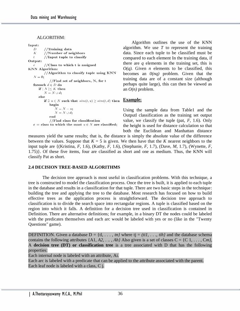
Data mining and Warehousing
| A.Thottarayaswamy M.C.A., M.Phil 36
ALGORITHM:
Algorithm outlines the use of the KNN
algorithm. We use T to represent the training
data. Since each tuple to be classified must be
compared to each element In the training data, if
there are q elements in the training set, this is
O(q). Given n elements to be classified, this
becomes an 0(nq) problem. Given that the
training data are of a constant size (although
perhaps quite large), this can then be viewed as
an O(n) problem.
Example:
Using the sample data from Table1 and the
Outputl classification as the training set output
value, we classify the tuple (pat, F, 1.6). Only
the height is used for distance calculation so that
both the Euclidean and Manhattan distance
measures yield the same results; that is, the distance is simply the absolute value of the difference
between the values. Suppose that K = 5 is given. We then have that the K nearest neighbors to the
input tuple are {(Kristina, F, 1.6), (Kathy, F, 1.6), (Stephanie, F, 1.7), (Dave, M, 1.7), (Wynette, F,
1.75)}. Of these five items, four are classified as short and one as medium. Thus, the KNN will
classify Pat as short.
2.4 DECISION TREE-BASED ALGORITHMS
The decision tree approach is most useful in classification problems. With this technique, a
tree is constructed to model the classification process. Once the tree is built, it is applied to each tuple
in the database and results in a classification for that tuple. There are two basic steps in the technique:
building the tree and applying the tree to the database. Most research has focused on how to build
effective trees as the application process is straightforward. The decision tree approach to
classification is to divide the search space into rectangular regions. A tuple is classified based on the
region into which it falls. A definition for a decision tree used in classification is contained in
Definition. There are alternative definitions; for example, in a binary DT the nodes could be labeled
with the predicates themselves and each arc would be labeled with yes or no (like in the "Twenty
Questions" game).
DEFINITION. Given a database D = {tl, . . . , tn} where tj = (ti1, . . ., tih} and the database schema
contains the following attributes {A1, A2, . .. , Ah} Also given is a set of classes C = {C 1, . . . , Cm},
A decision tree (DT) or classification tree is a tree associated with D that has the following
properties:
Each internal node is labeled with an attribute, Ai.
Each arc is labeled with a predicate that can be applied to the attribute associated with the parent.
Each leaf node is labeled with a class, C j.
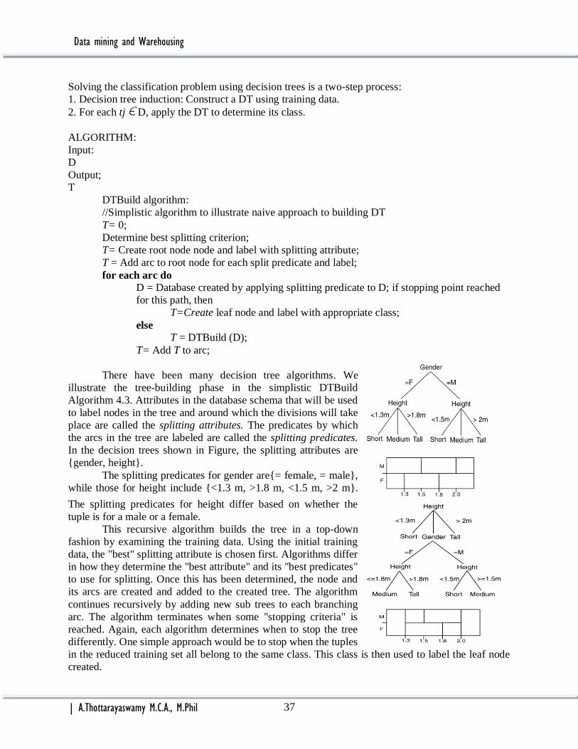
Data mining and Warehousing
| A.Thottarayaswamy M.C.A., M.Phil 37
Solving the classification problem using decision trees is a two-step process:
1. Decision tree induction: Construct a DT using training data.
2. For each tj D, apply the DT to determine its class.
ALGORITHM:
Input:
D
Output;
T
DTBuild algorithm:
//Simplistic algorithm to illustrate naive approach to building DT
T= 0;
Determine best splitting criterion;
T= Create root node node and label with splitting attribute;
T = Add arc to root node for each split predicate and label;
for each arc do
D = Database created by applying splitting predicate to D; if stopping point reached
for this path, then
T=Create leaf node and label with appropriate class;
else
T = DTBuild (D);
T= Add T to arc;
There have been many decision tree algorithms. We
illustrate the tree-building phase in the simplistic DTBuild
Algorithm 4.3. Attributes in the database schema that will be used
to label nodes in the tree and around which the divisions will take
place are called the splitting attributes. The predicates by which
the arcs in the tree are labeled are called the splitting predicates.
In the decision trees shown in Figure, the splitting attributes are
{gender, height}.
The splitting predicates for gender are{= female, = male},
while those for height include {<1.3 m, >1.8 m, <1.5 m, >2 m}.
The splitting predicates for height differ based on whether the
tuple is for a male or a female.
This recursive algorithm builds the tree in a top-down
fashion by examining the training data. Using the initial training
data, the "best" splitting attribute is chosen first. Algorithms differ
in how they determine the "best attribute" and its "best predicates"
to use for splitting. Once this has been determined, the node and
its arcs are created and added to the created tree. The algorithm
continues recursively by adding new sub trees to each branching
arc. The algorithm terminates when some "stopping criteria" is
reached. Again, each algorithm determines when to stop the tree
differently. One simple approach would be to stop when the tuples
in the reduced training set all belong to the same class. This class is then used to label the leaf node
created.

Data mining and Warehousing
| A.Thottarayaswamy M.C.A., M.Phil 38
Note that the major factors in the performance of the DT building algorithm are the size of the
training set and how the best splitting attribute is chosen. The following issues are faced by most DT
algorithms:
Choosing splitting attributes: Which attributes to use for splitting attributes impacts the
performance applying the built DT. Some attributes are better than others. In the data shown in
Table, the name attribute definitely should not be used and the gender mayor may not be used. The
choice of attribute involves not only an examination of the data in the training set but also the
informed input of domain experts.
Ordering of splitting attributes: The order in which the attributes are chosen is also
important. In Figure the gender attribute is chosen first. Alternatively, the height attribute could be
chosen first. As seen in Figure, in this case the height attribute must be examined a second time,
requiring unnecessary comparisons.
Splits: Associated with the ordering of the attributes is the number of splits to take. With
some attributes, the domain is small, so the number of splits is obvious based on the domain (as with
the gender attribute). However, if the domain is continuous or has a large number of values, the
number of splits to use is not easily determined.
Tree structure: To improve the performance of applying the tree for classification, a
balanced tree with the fewest levels is desirable. However, in this case, more complicated
comparisons with multi way branching may be needed. Some algorithms build only binary trees.
Stopping criteria: The creation of the tree definitely stops when the training data are perfectly
classified. There may be situations when stopping earlier would be desirable to prevent the creation
of larger trees. This is a trade-off between accuracy of classification and performance. In addition,
stopping earlier may be performed to prevent over fitting. It is even conceivable that more levels than
needed would be created in a tree if it is known that there are data distributions not represented in the
training data.
Training data: The structure of the DT created depends on the training data. If the training
data set is too small, then the generated tree might not be specific enough to work properly with the
more general data. If the training data set is too large, then the created tree may over fit.
Pruning: Once a tree is constructed, some modifications to the tree might be needed to
improve the performance of the tree during the classification phase. The pruning phase might remove
redundant comparisons or remove sub trees to achieve better performance.
2.4.1 ID3
The ID3 technique to building a decision tree is based on information theory and attempts
to minimize the expected number of comparisons. The basic idea of the induction algorithm is to
ask questions whose answers provide the most information. This is similar to the intuitive
approach taken by adults when playing the "Twenty Questions" game. The first question an adult
might ask could be "Is the thing alive?" while a child might ask "Is it my Daddy?" The first
question divides the search space into two large search domains, while the second performs little
division of the space.
The basic strategy used by ID3 is to choose splitting attributes with-the highest
information gain first. The amount of information associated with an attribute value is related to
the probability of occurrence. Looking at the "Twenty Questions" example, the child's question
divides the search space into two sets. One set (Daddy) has an infinitesimal probability associated
with it and the other set is almost certain, while the question the adult makes divides the search
space into two subsets with almost equal probability of occurring. The concept used to quantify
information is called entropy. Entropy is used to measure the amount of uncertainty or surprise
or randomness in a set of data. Certainly, when all data in a set belong to a single class, there is
no uncertainty. In this case the entropy is zero.

Data mining and Warehousing
| A.Thottarayaswamy M.C.A., M.Phil 39
The objective of decision tree classification is to iteratively partition the given data set
into subsets where all elements in each final subset belong to the same class. In Figure (a, b, and
c) will help to explain the concept. Figure (a) shows log (l/p) as the probability p ranges from 0 to
1. This intuitively shows the amount of surprise based on the probability. When P = 1, there is no
surprise. This means that if an event has a probability of I and you are told that the event
occurred, you would not be surprised. As p -> 0, the surprise increases. When we deal with a
divide and conquer approach such as that used with decision trees, the division results in multiple
probabilities whose sum is 1. In the "Twenty Questions" game, the P (Daddy) < P (~.Daddy) and
P(Daddy) + P(~Daddy) = 1. To measure the information associated with this division, we must be
able to combine the information associated with both events. That is, we must be able to calculate
the average information associated with the division. This can be performed by adding the two
values together and taking into account the probability that each occurs. Figure (b) shows the
function p log (l/p),
Which is the expected information based on probability of an event. To determine the expected
information associated with two events, we add the individual values together. This function p log
(l/p) + (l-p) log (l/(l- p)) is plotted in Figure (c). Note that the maximum occurs when the two
probabilities are equal. This supports our intuitive idea that the more sophisticated questions posed
by the adult are better than those posed by the child. The formal definition of entropy is shown in
Definition. The value for entropy is between 0 and 1 and reaches a maximum when the probabilities
are all the same.
DEFINITION: Given probabilities P1, P2, ..., Ps where L:f=1 Pi = I, entropy is defined as
Given a database state, D, H(D) finds the amount of order (or lack thereof). That state. When
that state is split into s new states S = {D1, D2,..., Ds}, we can again look at the entropy of those
states. Each step in ID3 chooses the state that orders splitting the most. A database state is completely
ordered if all tuples in it are in the same class. ID3 chooses the splitting attribute with the highest
gain in information, where gain is defined as the difference between how much information is needed
to make a correct classification before the split versus how much information is needed after the split.
Certainly, the split should reduce the information needed by the largest amount. This is calculated by
determining the differences between the entropies of the original dataset and the weighted sum of the
entropies from each of the subdivided datasets. The entropies of the split datasets are weighted by the
fraction of the dataset being placed in that division. The ID3 algorithm calculates the gain of a
particular split by the following formula:
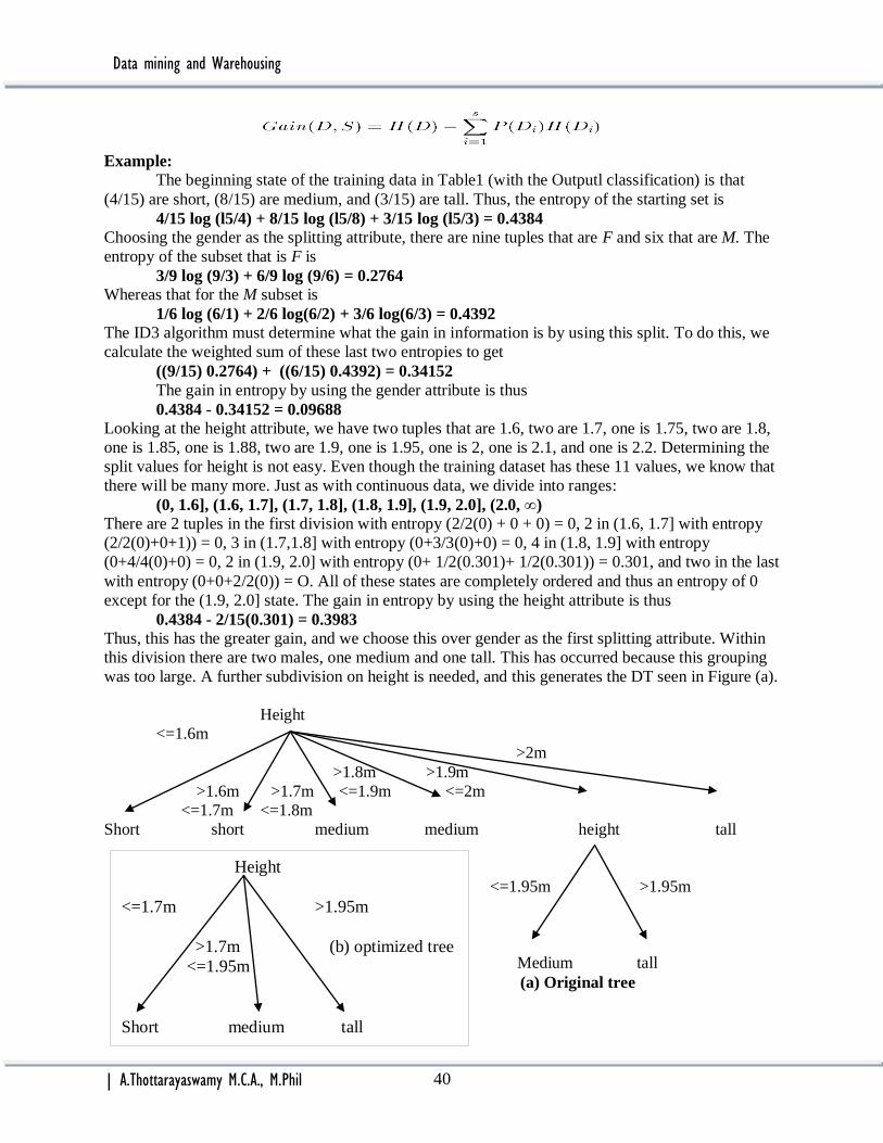
Data mining and Warehousing
| A.Thottarayaswamy M.C.A., M.Phil 40
Example:
The beginning state of the training data in Table1 (with the Outputl classification) is that
(4/15) are short, (8/15) are medium, and (3/15) are tall. Thus, the entropy of the starting set is
4/15 log (l5/4) + 8/15 log (l5/8) + 3/15 log (l5/3) = 0.4384
Choosing the gender as the splitting attribute, there are nine tuples that are F and six that are M. The
entropy of the subset that is F is
3/9 log (9/3) + 6/9 log (9/6) = 0.2764
Whereas that for the M subset is
1/6 log (6/1) + 2/6 log(6/2) + 3/6 log(6/3) = 0.4392
The ID3 algorithm must determine what the gain in information is by using this split. To do this, we
calculate the weighted sum of these last two entropies to get
((9/15) 0.2764) + ((6/15) 0.4392) = 0.34152
The gain in entropy by using the gender attribute is thus
0.4384 - 0.34152 = 0.09688
Looking at the height attribute, we have two tuples that are 1.6, two are 1.7, one is 1.75, two are 1.8,
one is 1.85, one is 1.88, two are 1.9, one is 1.95, one is 2, one is 2.1, and one is 2.2. Determining the
split values for height is not easy. Even though the training dataset has these 11 values, we know that
there will be many more. Just as with continuous data, we divide into ranges:
(0, 1.6], (1.6, 1.7], (1.7, 1.8], (1.8, 1.9], (1.9, 2.0], (2.0, ∞)
There are 2 tuples in the first division with entropy (2/2(0) + 0 + 0) = 0, 2 in (1.6, 1.7] with entropy
(2/2(0)+0+1)) = 0, 3 in (1.7,1.8] with entropy (0+3/3(0)+0) = 0, 4 in (1.8, 1.9] with entropy
(0+4/4(0)+0) = 0, 2 in (1.9, 2.0] with entropy (0+ 1/2(0.301)+ 1/2(0.301)) = 0.301, and two in the last
with entropy (0+0+2/2(0)) = O. All of these states are completely ordered and thus an entropy of 0
except for the (1.9, 2.0] state. The gain in entropy by using the height attribute is thus
0.4384 - 2/15(0.301) = 0.3983
Thus, this has the greater gain, and we choose this over gender as the first splitting attribute. Within
this division there are two males, one medium and one tall. This has occurred because this grouping
was too large. A further subdivision on height is needed, and this generates the DT seen in Figure (a).
Height
<=1.6m
>2m
>1.8m >1.9m
>1.6m >1.7m <=1.9m <=2m
<=1.7m <=1.8m
Short short medium medium height tall
<=1.95m >1.95m
Medium tall
(a) Original tree
Height
<=1.7m >1.95m
>1.7m (b) optimized tree
<=1.95m
Short medium tall

Data mining and Warehousing
| A.Thottarayaswamy M.C.A., M.Phil 41
2.4.2 C4.5 and C5.0
The decision tree algorithm C4.5 improves ill3 in the following ways:
Missing data: When the decision tree is built, missing data are simply ignored. That is, the
gain ratio is calculated by looking only at the other records that have a value for that attribute. To
classify a record with a missing attribute value, the value for that item can be predicted based on
what is known about the attribute values for the other records.
Continuous data: The basic idea is to divide the data into ranges based on the attribute
values for that item that are found in the training sample.
Pruning: There are two primary pruning strategies proposed in C4.5:
With sub tree replacement, a sub tree is replaced by a leaf node if this replacement
results in an error rate close to that of the original tree. Sub tree replacement works from the
bottom of the tree up to the root.
Another pruning strategy, called sub tree raising, replaces a sub tree by its most used
sub tree. Here a sub tree is raised from its current location to a node higher up in the tree.
Again, we must determine the increase in error rate for this replacement.
Rules: C4.5 allows classification via either decision trees or roles generated from them. In
addition, some techniques to simplify complex rules are proposed. One approach is to replace the
left-hand side of a rule by a simpler version if all records in the training set are treated identically. An
"otherwise" type of rule can be used to indicate what should be done if no other rules apply.
Splitting: The ill3 approach favors attributes with many divisions and thus may lead to over
fitting. In the extreme, an attribute that has a unique value for each tuple.
Approach uses the GainRatio as opposed to Gain. The GainRatio is defined as
2.4.3 CART
Classification and regression trees (CART) is a technique that generates a binary decision tree. As
with ID3, entropy is used as a measure to choose the best splitting attribute and criterion. Unlike ID3,
however, where a child is created for each subcategory, only two children are created. The splitting is
performed around what is determined to be the best split point. At each step, an exhaustive search is
used to determine the best split, where "best" is defined by
This formula is evaluated at the current node, t, and for each possible splitting attribute and criterion,
s. Here L and R are used to indicate the left and right sub trees of the current node in the tree. PL, PR
are the probability that a tuple in the training set will be on the left or right side of the tree. This is
defined as
| tuples in subtree |
| tuples in training set |
Data mining and Warehousing
| A.Thottarayaswamy M.C.A., M.Phil 42
Example:
The first step is to determine the split attribute and criterion for the first split. We again assume that
there are six sub ranges to consider with the height attribute. Using these ranges, we have the
potential split values of 1.6, 1.7, 1.8, 1.9, 2.0. We thus have a choice of six split points, which yield
the following goodness measures:
Ø(gender) = 2(6/15)(9/15)(2/15 + 4/15 + 3/15) = 0.224
Ø (1.6) = 0
Ø (1.7) = 2(2/15)(13/15)(0 + 8/15 + 3/15) = 0.169
Ø (1.8) = 2(5/15)(10/15)(4/15 + 6/15 + 3/15) = 0.385
Ø(1.9) = 2(9/15)(6/15)(4/15 + 2/15 + 3/15) = 0.256
Ø (2.0) = 2(12/15)(3/15)(4/15 + 8/15 + 3/15) = 0.32
2.4.4 Scalable DT Technique:
The SPRINT (Scalable Parallelizable Induction of decision Trees) algorithm addresses the
scalability issue by ensuring that the CART technique can be applied regardless of availability of
main memory. In addition, it can be easily parallelized. With SPRINT, a gini index is used to find the
best split. Here gini for a database D is defined as Gini(D) = 1 ∑p2j
Where P j is the frequency of class C j in D. The goodness of a split of D into subsets Dl and
D2 is defined by ginisplit (D) = (n1/n)(gini(D1)) + (n2/n)(gini(D2)) 2.5 NEURAL NETWORK-BASED ALGORITHMS
With neural networks (NNs) just as with decision trees, a model representing how to classify
any given database tuple is constructed. The activation functions typically are sigmoidal. When a
tuple must be classified, certain attribute values from that tuple are input into the directed graph at
the corresponding source nodes. There often is one sink node for each class. The output value that is
generated indicates the probability that the corresponding input tuple belongs to that class. The tuple
will then be assigned to the class with the highest probability of membership. The learning process
modifies the labeling of the arcs to better classify tuples. Given a starting structure and value for all
the labels in the graph, as each tuple in the training set is sent through the network, the projected
classification made by the graph can be compared with the actual classification. Based on (he
accuracy of the prediction, various labelings in the graph can change. This learning process continues
with all the training data or until the classification accuracy is adequate.
Solving a classification problem using NNs involves several steps:
1. Determine the number of output nodes as well as what attributes should be used as input. The
number of hidden layers (between the source and the sink nodes) also must be decided. This step is
performed by a domain expert.
2. Determine weights (labels) and functions to be used for the graph.
3. For each tuple the training set, propagate it through the network and evaluate the output
prediction to the actual result. If the prediction is accurate, adjust labels to ensure that this prediction
has a higher output weight the next time. If the prediction is not correct, adjust the weights to provide
a lower output value for this class.
4. For each tuple ti D, propagate ti through the network and make the appropriate
classification.

Data mining and Warehousing
| A.Thottarayaswamy M.C.A., M.Phil 43
There are many issues to be examined:
Attributes (number of source nodes): This is the same issue as determining which
attributes to use as splitting attributes. Number of hidden layers: In the simplest case, there is only
one hidden layer.
Number of hidden nodes: Choosing the best number of hidden nodes per hidden layer is
one of the most difficult problems when using NNs. There have been many empirical and theoretical
studies attempting to answer this question. The answer depends on the structure of the NN, types of
activation functions, training algorithm, and problem being solved. If too few hidden nodes are used,
the target function may not be learned (under fitting). If too many nodes are used, over fitting may
occur. Rules of thumb are often given that are based on the size of the training set.
Training data: As with DTs, with too much training data the NN may suffer from over
fitting, while too little and it may not be able to classify accurately enough.
Number of sinks: Although it is usually assumed that the number of output nodes is the
same as the number of classes, this is not always the case. For example, with two classes there could
only be one output node, with the resulting value being the probability of being in the associated
class. Subtracting this value from one would give the probability of being in the second class.
Interconnections: In the simplest case, each node is connected to all nodes in the next level.
Weights: The weight assigned to an arc indicates the relative weight between those two
nodes. Initial weights are usually assumed to be small positive numbers and are assigned randomly.
Activation functions: Many different types of activation functions can be used.
Learning technique: The technique for adjusting the weights is called the learning
technique. Although many approaches can be used, the most common approach is some form of
back propagation, which is discussed in a subsequent subsection.
Stop: The learning may stop when all the training tuples have propagated through the
network or may be based on time or error rate.
There are many advantages to the use of NNs for classification;
NNs are more robust than DTs because of weights.
The NN improves its performance by learning. This may continue even after the
training set has been applied.
The use of NNs can be parallelized for better performance.
There is a low error rate and thus a high degree of accuracy once the appropriate
training has been performed.
NNs are more robust than DTs in noisy environment.
NNs have many disadvantages:
NNs are difficult to understand. Nontechnical users may have difficulty
understanding how NNs works. While it is easy to explain decision trees, NNs are
much more difficult to understand.
Generating rules from NNs is not straightforward.
Input attribute values must be numeric.
Testing
Verification
As with DTs, over fitting may result.
The learning phase may fail to converge.
NNs may be quite expensive to use.

Data mining and Warehousing
| A.Thottarayaswamy M.C.A., M.Phil 44
2.5.1 Propagation
The normal approach used for processing is called propagation. Given a tuple of values input to the
NN, X = (Xl, . . . , Xh), one value is input at each node in the input layer. Then the summation and
activation functions are applied at each node, with an output value created for each output arc from
that node. These values are in turn sent to the subsequent nodes. This process continues until a tuple
of output values, Y = (Yl, . . . , Ym), is produced from the nodes in the output layer. The process of
propagation is shown in Algorithm using a neural network with one hidden layer. Here a hyperbolic
tangent activation function is used for the nodes in the hidden layer, while a sigmoid function is used
for nodes in the output layer. We assume that the constant c in the activation function has been
provided. We also use k to be the number of edges coming into a node.
Figure shows a very simple NN used to classify university students as short, medium, or tall. There
are two input nodes, one for the gender data and one for the height data. There are three output
nodes, each associated with one class and using a simple threshold activation function. Activation
function F3 is associated with the short class, F4 is associated with the medium class, and F5 is
associated with the tall class. In this case, the weights of each arc from the height node are 1. The
weights on the gender arcs are O. This implies that in this case the gender values are ignored. The
plots for the graphs of the three activation functions are shown.

Data mining and Warehousing
| A.Thottarayaswamy M.C.A., M.Phil 45
2.5. 2 NN Supervised Learning
The NN starting state is modified
based on feedback of its performance
with .the data in the training set. This
type of learning is referred to as
supervised because it is known a
priori what the desired output should
be Unsupervised learning can also be
performed if the output is not known.
With unsupervised approaches, no
external teacher set is used. A
training set may be provided, but no
labeling of the desired outcome is
included. In this case, similarities and
differences between different tuples
in the training set are uncovered. In
this chapter, we examine supervised
learning.
Supervised learning in an NN is the process of adjusting the arc weights based on its
performance with a tuple from the training set. The behavior of the training data is known a priori
and thus can be used to fine-tune the network for better behavior in future similar situations. Thus,
the training set can be used as a "teacher" during the training process. The output from the network is
compared to this known desired behavior. Algorithm outlines the steps required. One potential
problem with supervised learning is that the error may not be continually reduced. It would, of
course, be hoped that each iteration in the learning process reduces the error so that it is ultimately
below an acceptable level. However, this is not always the case. This may be due to the error
calculation technique or to the approach used for modifying the weights. This is actually the general
problem of NNs. They do not guarantee convergence or optirnality.
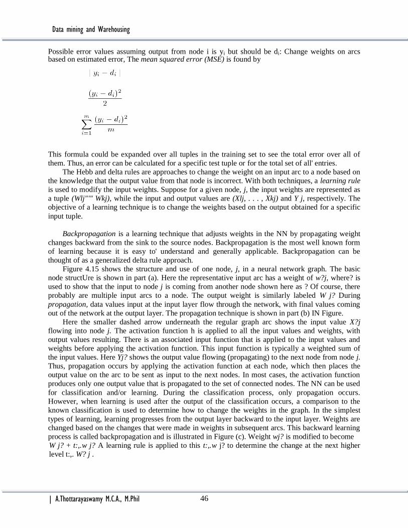
Data mining and Warehousing
| A.Thottarayaswamy M.C.A., M.Phil 46
Possible error values assuming output from node i is yi but should be di: Change weights on arcs based on estimated error, The mean squared error (MSE) is found by
This formula could be expanded over all tuples in the training set to see the total error over all of
them. Thus, an error can be calculated for a specific test tuple or for the total set of all' entries.
The Hebb and delta rules are approaches to change the weight on an input arc to a node based on
the knowledge that the output value from that node is incorrect. With both techniques, a learning rule
is used to modify the input weights. Suppose for a given node, j, the input weights are represented as
a tuple (Wlj"'" Wkj), while the input and output values are (Xlj, . . . , Xkj) and Y j, respectively. The
objective of a learning technique is to change the weights based on the output obtained for a specific
input tuple.
Backpropagation is a learning technique that adjusts weights in the NN by propagating weight
changes backward from the sink to the source nodes. Backpropagation is the most well known form
of learning because it is easy to' understand and generally applicable. Backpropagation can be
thought of as a generalized delta rule approach.
Figure 4.15 shows the structure and use of one node, j, in a neural network graph. The basic
node structUre is shown in part (a). Here the representative input arc has a weight of w?j, where? is
used to show that the input to node j is coming from another node shown here as ? Of course, there
probably are multiple input arcs to a node. The output weight is similarly labeled W j? During
propagation, data values input at the input layer flow through the network, with final values coming
out of the network at the output layer. The propagation technique is shown in part (b) IN Figure.
Here the smaller dashed arrow underneath the regular graph arc shows the input value X?j
flowing into node j. The activation function h is applied to all the input values and weights, with
output values resulting. There is an associated input function that is applied to the input values and
weights before applying the activation function. This input function is typically a weighted sum of
the input values. Here Yj? shows the output value flowing (propagating) to the next node from node j.
Thus, propagation occurs by applying the activation function at each node, which then places the
output value on the arc to be sent as input to the next nodes. In most cases, the activation function
produces only one output value that is propagated to the set of connected nodes. The NN can be used
for classification and/or learning. During the classification process, only propagation occurs.
However, when learning is used after the output of the classification occurs, a comparison to the
known classification is used to determine how to change the weights in the graph. In the simplest
types of learning, learning progresses from the output layer backward to the input layer. Weights are
changed based on the changes that were made in weights in subsequent arcs. This backward learning
process is called backpropagation and is illustrated in Figure (c). Weight wj? is modified to become
W j? + t:,.w j? A learning rule is applied to this t:,.w j? to determine the change at the next higher
level t:,. W? j .

Data mining and Warehousing
| A.Thottarayaswamy M.C.A., M.Phil 47
This algorithm changes weights by working backward from the output layer to the input layer.
There are two basic versions of this algorithm. With the batch or offline approach, the weights are
changed once after all tuples in the training set are applied and a total MSE is found. With the
incremental or online approach, the weights are changed after each tuple in the training set is applied.
The incremental technique is usually preferred because it requires less space and may actually
examine more potential solutions (weights), thus leading to a better solution. In this equation, 11 is
referred to as the learning parameter. It typically is found in the range (0, 1), although it may be
larger. This value determines how fast the algorithm learns.
Applying a learning rule back through multiple layers in the network may be difficult. Doing
this for the hidden layers is not as easy as doing it with the output layer. Overall, however, we are
trying to minimize the error at the output nodes, not at each node in the network. Thus, the approach
that is used is to propagate the output errors backward through the network.
2.5.3 Radial Basis Function Networks
A radial function or a radial basis function (RBF) is a class of functions whose value
decreases (or increases) with the distance from a central point. The Gaussian activation
function shown in Equation is an RBF with a central point of O. An RBF has a Gaussian
shape, and an RBF network is typically an NN with three layers. The input layer is used to
simply input the data. A Gaussian activation function is used at the hidden layer, while a

Data mining and Warehousing
| A.Thottarayaswamy M.C.A., M.Phil 48
linear activation function is used at the output layer. The objective is to have the hidden nodes
learn to respond only to a subset of the input, namely, that where the Gaussian function is
centered. This is usually accomplished via supervised learning. When RBF functions are used
as the activation functions on the hidden layer, the nodes can be sensitive to a subset of the
input values. Figure 4.18 shows the basic structure of an RBF unit with one output node.
2.5.4 Perceptrons
The simplest NN is called a perceptron. A perceptron is a single neuron with multiple inputs
and one output. The original perceptron proposed the use of a step activation function, but it is
more common to see another type of function such as a sigmoidal function. A simple
perceptron can be used to classify into two classes. Using a unipolar activation function, an
output of 1 would be used to classify into one class, while an output of 0 would be used to
pass in the other class.

Data mining and Warehousing
| A.Thottarayaswamy M.C.A., M.Phil 49
2.6 RULE-BASED ALGORITHMS
One straightforward way to perform classification is to generate if-then rules that cover all
cases. For example, we could have the following rules to determine classification of grades:
2.6.1 Generating Rules from a DT
The process to generate a rule from a DT is straightforward and is outlined in Algorithm. This
algorithm will generate a rule Jor each leaf node in the decision tree. All rules with the same
consequent could be combined together by ORing the antecedents of the simpler rules.
{ (Height:::: 1.6 m), Short)
«(Height> 1.6 m) /\ (Height:::: 1.7 m)), Short)
((Height> 1.7 m) /\ (Height:::: 1.8 m)), Medium)
((Height> (8 m) /\ (Height:::: 1.9 m)), Medium)
((Height> 1.9 m) /\ (Height:::: 2 m) /\ (Height:::: 1.95 m)), Medium)
((Height> 1.9 m) /\ (Height:::: 2 m) /\ (Height> 1.95 m)), Tall)
(Height> 2 m), Tall)}
An optimized version of these rules is then:
{(Height:::: 1.7 m), Short)
((Height> 1.7 m) /\ (Height:::: 1.95 m)), Medium) (
(Height> 1.95 m), Tall)}
4.6.2 Generating Rules from a Neural Net
To increase the understanding of an NN, classification rules may be derived from it. While the
source NN may still be used for classification, the derived rules can be used to verify or interpret the
network. The problem is that the rules do not explicitly exist. They are buried in the structwe of the
graph itself. In addition, if learning is still occurring, the rules themselves are dynamic. The rules
generated tend both to be more concise and to have a lower error rate than rules used with DTs. The
basic idea of the RX algorithm is to cluster output values. with the Associated hidden nodes and
input. A major Problem with rule extraction is the potential size that these rules should be. For
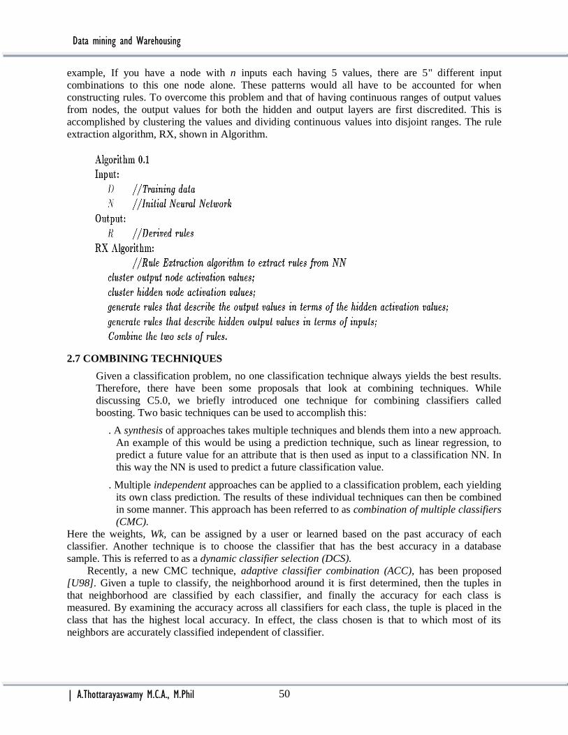
Data mining and Warehousing
| A.Thottarayaswamy M.C.A., M.Phil 50
example, If you have a node with n inputs each having 5 values, there are 5" different input
combinations to this one node alone. These patterns would all have to be accounted for when
constructing rules. To overcome this problem and that of having continuous ranges of output values
from nodes, the output values for both the hidden and output layers are first discredited. This is
accomplished by clustering the values and dividing continuous values into disjoint ranges. The rule
extraction algorithm, RX, shown in Algorithm.
2.7 COMBINING TECHNIQUES
Given a classification problem, no one classification technique always yields the best results.
Therefore, there have been some proposals that look at combining techniques. While
discussing C5.0, we briefly introduced one technique for combining classifiers called
boosting. Two basic techniques can be used to accomplish this:
. A synthesis of approaches takes multiple techniques and blends them into a new approach.
An example of this would be using a prediction technique, such as linear regression, to
predict a future value for an attribute that is then used as input to a classification NN. In
this way the NN is used to predict a future classification value.
. Multiple independent approaches can be applied to a classification problem, each yielding
its own class prediction. The results of these individual techniques can then be combined
in some manner. This approach has been referred to as combination of multiple classifiers
(CMC).
Here the weights, Wk, can be assigned by a user or learned based on the past accuracy of each
classifier. Another technique is to choose the classifier that has the best accuracy in a database
sample. This is referred to as a dynamic classifier selection (DCS).
Recently, a new CMC technique, adaptive classifier combination (ACC), has been proposed
[U98]. Given a tuple to classify, the neighborhood around it is first determined, then the tuples in
that neighborhood are classified by each classifier, and finally the accuracy for each class is
measured. By examining the accuracy across all classifiers for each class, the tuple is placed in the
class that has the highest local accuracy. In effect, the class chosen is that to which most of its
neighbors are accurately classified independent of classifier.

Data mining and Warehousing
| A.Thottarayaswamy M.C.A., M.Phil 51
3.1 INTRODUCTION
Clustering is similar to classification in that data are grouped. However, unlike classification,
the groups are not predefined. Instead, the grouping is accomplished by finding similarities between
data according to characteristics found in the actual data. The groups are called clusters. Some
authors view clustering as a special type of classification. In this text, however, we follow a more
conventional view in that the two are different. Many definitions for clusters have been proposed:
Set of like elements. Elements from different clusters are not alike.
The distance between points in a cluster is less than the distance between a point in the
cluster and any point outside it.
A term similar to clustering is database segmentation, where like tuples (records) in a
database are grouped together. This is done to partition or segment the database into components that
then give the user a more general view of the data. In this text, we do not differentiate between
segmentation and clustering. A simple example of clustering is found in Example. This example
illustrates the fact that determining how to do the clustering is not straightforward.
EXAMPLE
An international online catalog company wishes to group its customers based on common
features. Company management does not have any predefined labels for these groups. Based on the
outcome of the grouping, they will target marketing and advertising campaigns to the different
groups. The information they have about the customers includes income, age, and number of
children, marital status, and education. Table shows some tuples from this database for customers in
the United States. Depending on the type of advertising, not all attributes are important.
For example, suppose the advertising is for a special sale on children's clothes. We could
target the advertising only to the persons with children. One possible clustering is that shown by the
divisions of the table. The first group of people has young children and a high school degree, while
the second group is similar but have no children. The third group has both children and a college
degree. The last two groups have higher incomes and at least a college degree. The very last group
has children. Different clustering would have been found by examining age or marital status.
UNIT 3 – Clustering
3.1 Introduction
3.2 Similarity and Distance Measures
3.3 Outliers
3.4 Hierarchical algorithms
3.5 Partitional algorithms

Data mining and Warehousing
| A.Thottarayaswamy M.C.A., M.Phil 52
As illustrated in Figure, a given set of data may be clustered on different attributes. Here a
group of homes in a geographic area is shown. The first type of clustering is based on the location of
the home. Homes that are geographically close to each other are clustered together. In the second
clustering, homes are grouped based on the size of the house.
Clustering has been used in many application domains, including biology, medicine,
anthropology, marketing, and economics. Clustering applications include plant and animal
classification, disease classification, image processing, pattern recognition, and document retrieval.
One of the first domains in which clustering were used was biological taxonomy. Recent uses include
examining Web log data to detect usage patterns.
When clustering is applied to a real-world database, many interesting problems occur.
Outlier handling is difficult. Here the elements do not naturally fall into any cluster.
They can be viewed as solitary clusters. However, if a clustering algorithm attempts
to find larger clusters, these outliers will be forced to be placed in some cluster. This
process may result in the creation of poor clusters by combining two existing clusters
and leaving the outlier in its own cluster.
Dynamic data in the database implies that cluster membership may change over time.
Interpreting the semantic meaning of each cluster may be difficult. With classifica-
tion, the labeling of the classes is known ahead of time. However, with clustering,
this may not be the case. Thus, when the clustering process finishes creating a set of
clusters, the exact meaning of each cluster may not be obvious. Here is where a
domain expert is needed to assign a label or interpretation for each cluster.
There is no one correct answer to a clustering problem. In fact, many answers may be
found. The exact number of clusters required is not easy to determine. Again, a

Data mining and Warehousing
| A.Thottarayaswamy M.C.A., M.Phil 53
domain expert may be required. For example, suppose we have a set of data about
plants that have been collected during a field trip. Without any prior knowledge of
plant classification, if we attempt to divide this set of data into similar groupings, it
would not be clear how many groups should be created.
Another related issue is what data should be used for clustering. Unlike learning
during a classification process, where there is some a priori knowledge concerning
what the attributes of each classification should be, in clustering we have no
supervised learning to aid the process. Indeed, clustering can be viewed as similar to
unsupervised learning.
We can then summarize some basic features of clustering (as opposed to classification):
The (best) number of clusters is not known.
There may not be any a priori knowledge concerning the clusters.
Cluster results are dynamic.
The clustering Definition:
Given a database D={t1,t2,…,tn} of tuples and an integer value k, the Clustering
Problem is to define a mapping f:Dg{1,..,k} where each ti is assigned to one cluster
Kj, 1<=j<=k. A Cluster, Kj, contains precisely those tuples mapped to it.
Clustering Approaches
With hierarchical clustering, a nested set of clusters is created. Each level in the hierarchy
has a separate set of clusters. At the lowest level, each item is in its own unique cluster. At the
highest level, all items belong to the same cluster. With hierarchical clustering, the desired number of
clusters is not input.
With partitional clustering, the algorithm creates only one set of clusters. These approaches
use the desired number of clusters to drive how the final set is created. Traditional clustering
algorithms tend to be targeted to small numeric databases that fit into memory. There are, however,
more recent clustering algorithms that look at categorical data and are targeted to larger, perhaps
dynamic, databases. Algorithms targeted to larger databases may adapt to memory constraints by
either sampling the database or using data structures, which can be compressed or pruned to fit into
memory regardless of the size of the database. Clustering algorithms may also differ based on
whether they produce overlapping or nonoverlapping clusters. Even though we consider only
nonoverlapping clusters, it is possible to place an item in multiple clusters. In turn, nonoverlapping
clusters can be viewed as extrinsic or intrinsic.
Extrinsic techniques use labeling of the items to assist in the classification process. These
algorithms are the traditional classification supervised learning algorithms in which a special input
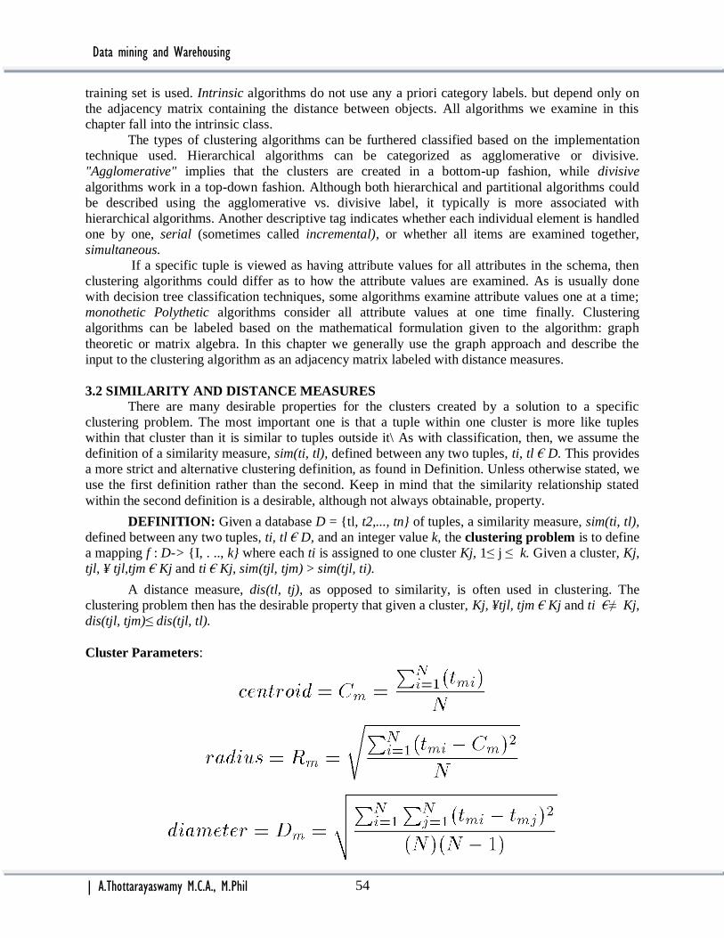
Data mining and Warehousing
| A.Thottarayaswamy M.C.A., M.Phil 54
training set is used. Intrinsic algorithms do not use any a priori category labels. but depend only on
the adjacency matrix containing the distance between objects. All algorithms we examine in this
chapter fall into the intrinsic class.
The types of clustering algorithms can be furthered classified based on the implementation
technique used. Hierarchical algorithms can be categorized as agglomerative or divisive.
"Agglomerative" implies that the clusters are created in a bottom-up fashion, while divisive
algorithms work in a top-down fashion. Although both hierarchical and partitional algorithms could
be described using the agglomerative vs. divisive label, it typically is more associated with
hierarchical algorithms. Another descriptive tag indicates whether each individual element is handled
one by one, serial (sometimes called incremental), or whether all items are examined together,
simultaneous.
If a specific tuple is viewed as having attribute values for all attributes in the schema, then
clustering algorithms could differ as to how the attribute values are examined. As is usually done
with decision tree classification techniques, some algorithms examine attribute values one at a time;
monothetic Polythetic algorithms consider all attribute values at one time finally. Clustering
algorithms can be labeled based on the mathematical formulation given to the algorithm: graph
theoretic or matrix algebra. In this chapter we generally use the graph approach and describe the
input to the clustering algorithm as an adjacency matrix labeled with distance measures.
3.2 SIMILARITY AND DISTANCE MEASURES
There are many desirable properties for the clusters created by a solution to a specific
clustering problem. The most important one is that a tuple within one cluster is more like tuples
within that cluster than it is similar to tuples outside it\ As with classification, then, we assume the
definition of a similarity measure, sim(ti, tl), defined between any two tuples, ti, tl € D. This provides
a more strict and alternative clustering definition, as found in Definition. Unless otherwise stated, we
use the first definition rather than the second. Keep in mind that the similarity relationship stated
within the second definition is a desirable, although not always obtainable, property.
DEFINITION: Given a database D = {tl, t2,..., tn} of tuples, a similarity measure, sim(ti, tl),
defined between any two tuples, ti, tl € D, and an integer value k, the clustering problem is to define
a mapping f : D-> {I, . .., k} where each ti is assigned to one cluster Kj, 1≤ j ≤ k. Given a cluster, Kj,
tjl, ¥ tjl,tjm € Kj and ti € Kj, sim(tjl, tjm) > sim(tjl, ti).
A distance measure, dis(tl, tj), as opposed to similarity, is often used in clustering. The
clustering problem then has the desirable property that given a cluster, Kj, ¥tjl, tjm € Kj and ti €≠ Kj,
dis(tjl, tjm)≤ dis(tjl, tl).
Cluster Parameters:

Data mining and Warehousing
| A.Thottarayaswamy M.C.A., M.Phil 55
Distance Between Clusters
Single Link: smallest distance between points
Complete Link: largest distance between points
Average Link: average distance between points
Centroid: distance between centroids
3.3 OUTLIERS
As mentioned earlier, outliers are sample points with values much different from those of
the remaining set of data. Outliers may represent errors in the data (perhaps a mal functioning
sensor recorded an incorrect data value) or could be correct data values that are simply much
different from the remaining data.
A person who is 2.5 meters tall is much taller than most people. In analyzing the height of
individuals, this value probably would be viewed as an outlier. Some clustering techniques do not
perform well with the presence of outliers. This problem is illustrated in Figure. Here if three
clusters are found (solid line), the outlier will occur in a cluster by itself. However, if two clusters
are found (dashed line), the two (obviously) different sets of data will be placed in one cluster
because they are closer together than the outlier. This problem is complicated by the fact that many
clustering algorithms actually have as input the number of desired clusters to be found.
Clustering algorithms may actually find and remove outliers to ensure that they perform
better. However, care must be taken in actually removing outliers. For example, suppose that the
data mining problem is to predict flooding. Extremely high water level values occur very
infrequently, and when compared with the normal water level values may seem to be outliers.
However, removing these values may not allow the data mining algorithms to work effectively
because there would be no data that showed that floods ever actually occurred.
Outlier detection, or outlier mining, is the process of identifying outliers in a set of data.
Clustering, or other data mining, algorithms may then choose to remove or treat these values
differently. Some outlier detection techniques are based on statistical techniques. These usually
assume that the set of data follows a known distribution and that outliers can be detected by well-
known tests such as discordancy tests. However, these tests are not very realistic for real-world data
because real-world data values may not follow well-defined data distributions. Also, most of these
tests assume a single attribute value, and many attributes are involved in real-world datasets.
Alternative detection techniques may be based on distance measures.

Data mining and Warehousing
| A.Thottarayaswamy M.C.A., M.Phil 56
3.4 HIERARCHICAL ALGORITHMS
As mentioned earlier, hierarchical clustering algorithms actually creates sets of clusters.
Hierarchical algorithms differ in how the sets are created. A tree data structure, called a dendrogram,
can be used to illustrate the hierarchical clustering technique and the sets of different clusters. The
root in a dendrogram tree contains one cluster where all element& are together. The leaves in the
dendrogram each consist of a single element cluster. Internal nodes in the dendrogram represent new
clusters formed by merging the clusters that appear as its children in the tree.
Each level in the tree is associated with the distance measure that was used to merge the
clusters. All clusters created at a particular level were combined because the children clusters had a
distance between them less than the distance value associated with this level in the tree. A
dendrogram for Example is seen in following Figure.
EXAMPLE Following Figure shows six elements, {A, B, C, D, E, F}, to be clustered. Parts (a) to (e) of
the figure show five different sets of "clusters. In part (a) each cluster is viewed to consist of a single
element. Part (b) illustrates four clusters. Here there are two sets of two-element clusters. These
clusters are formed at this level because these two elements are closer to each other than any of the
other elements. Part (c) shows a new cluster formed by adding a close element to one of the two-
element clusters. In part (d) the two-element and three-element clusters are merged to give a five-
element cluster. This is done because these two clusters are closer to each other than to the remote
element cluster, {F}. At the last stage, part (e), all six elements are merged.
The space complexity for hierarchical algorithms is O(n2) because this is the space required
for the adjacency matrix. The space required for the dendrogram is O(kn), which is much less than
0,(n2). The time complexity for hierarchical algorithms is O(kn2) because there is one iteration for
each level in the dendrogram. Depending on the specific algorithm, however, this could actually be
O(maxd n2) where maxd is the maximum distance between points. Different algorithms may actually
merge the closest clusters from the next lowest level or simply create new clusters at each level with
progressively larger distances.

Data mining and Warehousing
| A.Thottarayaswamy M.C.A., M.Phil 57
Hierarchical techniques are well suited for many clustering applications that naturally exhibit
a nesting relationship between clusters. For example, in biology, plant and animal taxonomies could
easily be viewed as a hierarchy of clusters.
3.4.1 Agglomerative Algorithms
Agglomerative algorithms start with each individual item in its own cluster and iteratively
merge clusters until all items belong in one cluster. Different agglomerative algorithms differ in how
the clusters are merged at each level. Clustering Algorithm illustrates the typical agglomerative
clustering algorithm. It assumes that a set of elements and distances between them is given as input.
We use an n x n vertex adjacency matrix, A, as input. Here the adjacency matrix, A, contains a
distance value rather than a simple Boolean value: A[i, j] = dis(ti, tj). The output of the algorithm is a
dendrogram, DE, which we represent as a set of ordered triples (d, k, K) where d is the threshold
distance, k is the number of clusters, and K is the set of clusters. The dendrogram in Figure 5.7(a)
would be represented by the following:
{(O, 5, {{A}, {B}, {C}, {D}, {E}}), (1,3, {{A, B}, {C, D}, {E}}) (2,2, {{A, B, C, D}, (E}}),
(3, 1, ({A, B, C, D, E}})}
ALGORITHM:
This algorithm uses a procedure called NewClusters to determine how to create the next level
of clusters from the previous level. This is where the different types of agglomerative algorithms
differ. It is possible that only two clusters from the prior level are merged or that multiple clusters are
merged. Algorithms also differ in terms of which clusters are merged when there are several clusters
with identical distances. In addition, the technique used to determine the distance between clusters
may vary. Single link, complete link, and average link techniques are perhaps the most well known
agglomerative techniques based on well-known graph theory concepts.
All agglomerative approaches experience excessive time and space constraints. The space
required for the adjacency matrix is O(n2) where there are n items to cluster. Because of the iterative

Data mining and Warehousing
| A.Thottarayaswamy M.C.A., M.Phil 58
nature of the algorithm, the matrix (or a subset of it) must be accessed multiple times. The simplistic
algorithm provided in Algorithm 5.1 performs at most maxd examinations of this matrix where maxd
is the largest distance between any two points. In addition the complexity of the NewClusters
procedure could be expensive. This is a potentially severe problem in large databases. Another issue
with the agglomerative approach is that it is not incremental. Thus, when new elements are added or
old ones are removed or changed, the entire algorithm must be rerun. More recent incremental
variations, as discussed later in this text, address this problem.
Single Link Technique: The single link technique is based on the idea of finding maximal
connected components in a graph. A connected component is a graph in which there exists a path
between any two vertices. With the single link approach, two clusters are merged if there is at least
one edge that connects the two clusters; that is, if the minimum distance between any two points is
less than or equal to the threshold distance being considered. For this reason, it is often called the
nearest neighbor clustering technique. Following example illustrates this process.
EXAMPLE:
Table contains five sample data items with the distance between the elements indicated in the
table entries. When viewed as a graph problem, Figure (a) shows the general graph with all edges
labeled with the respective distances. To understand the idea behind the hierarchical approach, we
show several graph variations in Figures (b), (c), (d), and (e). Figure 5.6(b) shows only those edges
with a distance of I or less. There are only two edges. The first level of single link clustering then
will combine the connected clusters (single elements from the first phase), giving three clusters:
{A,B}, {C,D}, and {E}. During the next level of clustering, we look at edges with a length of 2 or
less. The graph representing this threshold distance is shown in Figure (c).
Note that we now have an edge (actually three) between the two clusters {A,B} and {C,D}.
Thus, at this level of the single link clustering algorithm, we merge these two clusters to obtain a
total of two clusters: {A,B,C,D} and {E}. The graph that is created with a threshold distance of 3 is
shown in Figure (d). Here the graph is connected, so the two clusters from the last level are merged
into one large cluster that contains all elements. The dendrogram for this single link example is
shown in Figure (a). The labeling on the right-hand side shows the threshold distance used to merge
the clusters at each level.
MST for example

Data mining and Warehousing
| A.Thottarayaswamy M.C.A., M.Phil 59
Dendrograms for above example
ALGORITHM:
Complete Link Algorithm:
Although the complete link algorithm is similar to the single link algorithm, it looks for
cliques rather than connected components. A clique is a maximal graph in which there is an edge
between any two vertices. Here a procedure is used to find the maximum distance between any
clusters so that two clusters are merged if the maximum distance is less than or equal to the distance
threshold. In this algorithm, we assume the existence of a procedure, clique, which finds all cliques
in a graph. As with the single link algorithm, this is expensive because it is an O(n2) algorithm.
Clusters found with the complete link method tend to be more compact than those found
using the single link technique. Using the data found in pervious Example, Figure (b) shows the

Data mining and Warehousing
| A.Thottarayaswamy M.C.A., M.Phil 60
dendrogram created. A variation of the complete link algorithm is called the farthest neighbor
algorithm. Here the closest clusters are merged where the distance is the smallest measured by
looking at the maximum distance between any two points.
Average Link:
The average link technique merges two clusters if the average distance between any two
points in the two target clusters is below the distance threshold. The algorithm used here is slightly
different from that found in single and complete link algorithms because we must examine the
complete graph (not just the threshold graph) at each stage.
3.4.2 Divisive Clustering:
With divisive clustering, all items are initially placed in one cluster and clusters are
repeatedly split in two until all items are in their own cluster. The idea is to split up clusters where
some elements are not sufficiently close to other elements.
One simple example of a divisive algorithm is based on the MST version of the single link
algorithm. Here, however, we cut out edges from the MST from the largest to the smallest. Looking
at MST Figure, we would start with a cluster containing a1l items: {A, B, C, D, E}. Looking at the
MST, we see that the largest edge is between D and E. Cutting this out of the MST, we then split the
one cluster into two: {E} and {A, B, C, D}. Next we remove the edge between Band C. This splits the
one large cluster into two: {A, B} and {C, D}. These will then be split at the next step. The order
depends on how a specific implementation would treat identical values. Looking at the dendrogram
in Figure (a), we see that we have created the same set of clusters as with the agglomerative
approach, but in reverse order.
3.5 PARTITIONAL ALGORITHMS
Nonhierarchical or partitional clustering creates the clusters in one step as opposed to several
steps. Only one set of clusters is created, although several different sets of clusters may be created
internally within the various algorithms. Since only one set of clusters is output, the user must input
the desired number, k, of clusters. In addition, some metric or criterion function is used to determine
the goodness of any proposed solution. This measure of quality could be the average distance
between clusters or some other metric. The solution with the best value for the criterion function is
the clustering solution used. One common measure is a squared error metric, which measures the
squared distance from each point to the Centroid for the associated cluster:
k
∑ ∑ dis(Cm, tmi)2
m=1 tmi €Km
There are 11,259,666,000 different ways to cluster 19 items into 4 clusters. Thus, most algorithms
look only at a small subset of all the clusters using some strategy to identify sensible clusters.
Because of the plethora of partitional algorithms, we will look at only a representative few. We have
chosen some of the most well known algorithms as well as some others that have appeared recently
in the literature.
3.5.1 Minimum Spanning Tree
Since we have agglomerative and divisive algorithms based on the use of an MST, we also present a
partitional MST algorithm. This is a very simplistic approach, but it illustrates how partitional
algorithms work. The algorithm is shown in following Algorithm. Since the clustering problem is to
define a mapping, the output of this algorithm shows the clusters as a set of ordered pairs (ti, j)
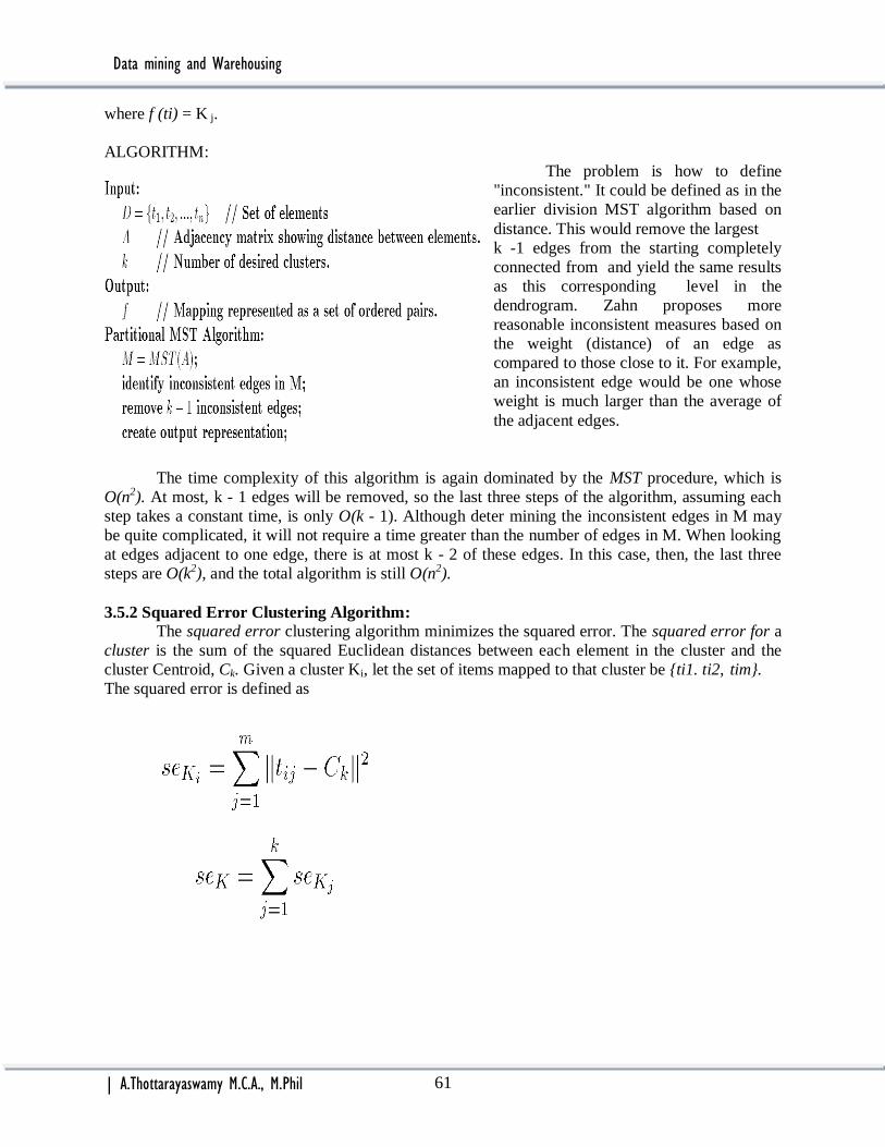
Data mining and Warehousing
| A.Thottarayaswamy M.C.A., M.Phil 61
where f (ti) = K j.
ALGORITHM:
The problem is how to define
"inconsistent." It could be defined as in the
earlier division MST algorithm based on
distance. This would remove the largest
k -1 edges from the starting completely
connected from and yield the same results
as this corresponding level in the
dendrogram. Zahn proposes more
reasonable inconsistent measures based on
the weight (distance) of an edge as
compared to those close to it. For example,
an inconsistent edge would be one whose
weight is much larger than the average of
the adjacent edges.
The time complexity of this algorithm is again dominated by the MST procedure, which is
O(n2). At most, k - 1 edges will be removed, so the last three steps of the algorithm, assuming each
step takes a constant time, is only O(k - 1). Although deter mining the inconsistent edges in M may
be quite complicated, it will not require a time greater than the number of edges in M. When looking
at edges adjacent to one edge, there is at most k - 2 of these edges. In this case, then, the last three
steps are O(k2), and the total algorithm is still O(n2).
3.5.2 Squared Error Clustering Algorithm:
The squared error clustering algorithm minimizes the squared error. The squared error for a
cluster is the sum of the squared Euclidean distances between each element in the cluster and the
cluster Centroid, Ck. Given a cluster Ki, let the set of items mapped to that cluster be {ti1. ti2, tim}.
The squared error is defined as

Data mining and Warehousing
| A.Thottarayaswamy M.C.A., M.Phil 62
ALGORITHM: Squared error.
3.5.3 K-Means Clustering
K-means is an iterative clustering algorithm in which items are moved among sets of clusters
until desired set is reached. As such, it may be viewed as a type of squared error algorithm, although
the convergehce criteria need not be defined based on the squared error. A high degree of similarity
among elements in clusters is obtained, while a high degree of dissimilarity among elements in
different clusters is achieved simultaneously. The cluster mean of Ki = {ti1, ti2,…tim} is defined as
mi = (1/m)(ti1 + … + tim)
ALGORITHM:

Data mining and Warehousing
| A.Thottarayaswamy M.C.A., M.Phil 63
EXAMPLE:
Given: {2,4,10,12,3,20,30,11,25}, k=2
Randomly assign means: m1=3,m2=4
K1={2,3}, K2={4,10,12,20,30,11,25}, m1=2.5,m2=16
K1={2,3,4},K2={10,12,20,30,11,25}, m1=3,m2=18
K1={2,3,4,10},K2={12,20,30,11,25}, m1=4.75,m2=19.6
K1={2,3,4,10,11,12},K2={20,30,25}, m1=7,m2=25
Stop as the clusters with these means are the same.
3.5.4 Nearest Neighbor Algorithm
An algorithm similar to the single link technique is called the nearest neighbor algorithm.
With this serial algorithm, items are iteratively merged into the existing clusters that are closest. In
this algorithm a threshold, t, is used to determine if items will be added to existing clusters or if a
new cluster is created.
ALGORITHM:
EXAMPLE:
Initially, A is placed in a cluster by itself, so we have Kl = {A}. We then look at B to decide if
it should be added to Kl or be placed in a new cluster. Since dis(A, B) = 1, which is less than the
threshold of 2, we place B in Kl to get K1 = {A. B}. When looking at C, we see that its distance to
both A and B is 2, so we add it to the cluster to get Kl = {A, B. C}. The dis(D, C) = 1 < 2, so we get
K1 = {A, B, C, D}. Finally, looking at E, we see that the closest item in K 1 has a distance of 3, which
is greater than 2, so we place it in its own cluster: K2 = {E}.

Data mining and Warehousing
| A.Thottarayaswamy M.C.A., M.Phil 64
3.5.5 PAM Algorithm
The PAM (partitioning around medoids) algorithm, also called the K-medoids algorithm,
represents a cluster by a medoid. Using a medoid is an approach that handles outliers well. The PAM
algorithm is shown in Algorithm. Initially, a random set of k items is taken to be the set of medoids.
Then at each step, all items from the input dataset that are not currently medoids are examined one by
one to see if they should be medoids. That is, the algorithm determines whether there is an item that
should replace one of the existing medoids. By looking at all pairs of medoid, non-medoid objects,
the algorithm chooses the pair that improves the overall quality of the clustering the best and
exchanges them. Quality here is measured by the sum of all distances from a non-medoid object to
the medoid for the cluster it is in. An item is assigned the cluster represented by the medoid to which
it is closest (minimum distance). We assume that Ki is the cluster represented by medoid. Suppose ti
is a current medoid and we wish to determine whether it should be exchanged with a non-medoid th
.We wish to do this swap only if the overall impact to the cost (sum of the distances to cluster
medoids) represents ail improvement.
We use Cjih to be the cost change for an item tj associated with swapping medoid ti with non-
medoid th The cost is the change to the sum of all distances from items to their cluster medoids.
There are four cases that must be examined when calculating this cost:
ALGORITHM:
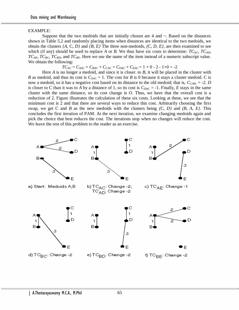
Data mining and Warehousing
| A.Thottarayaswamy M.C.A., M.Phil 65
EXAMPLE:
Suppose that the two medoids that are initially chosen are 4 and ~. Based on the distances
shown in Table 5.2 and randomly placing items when distances are identical to the two medoids, we
obtain the clusters {A, C, D} and {B, E} The three non-medoids, (C, D, E}, are then examined to see
which (if any) should be used to replace A or B. We thus have six costs to determine: TCAC, TCAD,
TCAE, TCBC, TCBD, and TCBE. Here we use the name of the item instead of a numeric subscript value.
We obtain the following:
TCAC = CAAC + CBAC + CCAC + CDAC + CEAC = 1 + 0 - 2 - 1+0 = -2
Here A is no longer a medoid, and since it is closer. to B, it will be placed in the cluster with
B as medoid, and thus its cost is CAAC = 1. The cost for B is 0 because it stays a cluster medoid. C is
now a medoid, so it has a negative cost based on its distance to the old medoid; that is, CCAB. = -2. D
is closer to C than it was to A by a distance of 1, so its cost is CDAC = -1. Finally, E stays in the same
cluster with the same distance, so its cost change is O. Thus, we have that the overall cost is a
reduction of 2. Figure illustrates the calculation of these six costs. Looking at these, we see that the
minimum cost is 2 and that there are several ways to reduce this cost. Arbitrarily choosing the first
swap, we get C and B as the new medoids with the clusters being (C, D} and (B, A, E}. This
concludes the first iteration of PAM. At the next iteration, we examine changing medoids again and
pick the choice that best reduces the cost. The iterations stop when no changes will reduce the cost.
We leave the rest of this problem to the reader as an exercise.

Data mining and Warehousing
| A.Thottarayaswamy M.C.A., M.Phil 66
3.5.6 Bond Energy Algorithm
The bond energy algorithm (BEA) was developed and has been used in the database design
area to determine how to group data and how to physically place data on a disk. It can be used to
cluster attributes based on usage and then perform logical or physical design accordingly. With
BEA, the affinity (bond) between database attributes is based on common usage. This bond is used
by the clustering algorithm as a similarity measure the actual measure counts the number of times
the two attributes are used together in a given time. To find this, all common queries must be
identified.
The idea is that attributes that are used together form a cluster and should be stored
together. In a distributed database, each resulting cluster is called a vertical fragment and may be
stored at different sites from other fragments. The basic steps of this clustering algorithm are:
1. Create an attribute affinity matrix in which each entry indicates the affinity between the two
associate attributes. The entries in the similarity matrix are based on the frequency of common
usage of attribute pairs.
2. The BEA then converts this similarity matrix to a BOND matrix in which the entries represent a
type of nearest neighbor bonding based on probability of co-access. The BEA algorithm
rearranges rows or columns so that similar attributes appear close together in the matrix.
3. Finally, the designer draws boxes around regions in the matrix with high similarity.
ALGORITHM:
Clustering affinity matrix for BEA
:

Data mining and Warehousing
| A.Thottarayaswamy M.C.A., M.Phil 67
3.5.7 Clustering with Genetic Algorithms
There have been clustering techniques based on the use of genetic algorithms. To determine
how to perform clustering. with genetic algorithms, we first must determine how to represent each
cluster. One simple approach would be to use a bit-map representation for each possible cluster. So,
given a database with four items, {A, B, C, D}, we would represent one solution to creating two
clusters as 1001 and 0110. This represents the two clusters {A, D} and {B, C}.
Algorithm shows one possible iterative refinement technique for clustering that uses a genetic
algorithm. The approach is similar to that in the squared error approach in that an initial random
solution is given and successive changes to this converge on a local optimum. A new solution is
generated from the previous solution using crossover and mutation operations. Our algorithm shows
only crossover. The use of crossover to create a new solution from a previous solution is shown in
following Example. The new "solution" must be created in such a way that it represents a valid k
clustering. A fitness function must be used and may be defined based on an inverse of the squared
error. Because of the manner in which crossover works, genetic clustering algorithms perform a
global search rather than a local search of potential solutions.
ALGORITHM:
INPUT
D = {t1, t2, … , tn} //set of elements
k // number of desired clusters
OUTPUT
k // set of clusters
GA clustering algorithm:
Randomly create an initial solution;
Repeat
Use crossover to create a new solution;
Until termination criteria is met;
EXAMPLE
Suppose a database contains the following eight items {A, B, C, D, E, F, G, H}, which are to
be placed into three clusters. We could initially place the items into the three clusters {A, C, E},
{B, F}, and {D, G, H}, which are represented by 10101000, 01000100, and 00010011, respectively.
Suppose we choose the first and third individuals as parents and do a simple crossover at point 4.
This yields the new solution: 00011000, 01000100, and 10100011.
3.5.8 Clustering with Neural Networks
Neural networks (NNs) that use unsupervised learning attempt to find features in the data that
characterize the desired output. They look for cluster of like data. These types of NNs are often
called self-organizing neural networks. There are two basic types of unsupervised learning:
noncompetitive and competitive.
With the noncompetitive or Hebbian learning, the weight between two nodes is changed to be
proportional to both output values. That is ∆wji = ηyjyi
With competitive learning, nodes are allowed to compete and the winner takes all. This
approach usually assumes a two-layer NN in which all nodes from one layer are connected to all
nodes in the other layer. As training occurs, nodes in the output layer become associated with certain
tuples in the input dataset. Thus, this provides a grouping of these tuples together into a cluster.
Imagine every input tuple having each attribute value input to a specific input node in the NN. The
number of input nodes is the same as the number of attributes. We can thus associate each weight to

Data mining and Warehousing
| A.Thottarayaswamy M.C.A., M.Phil 68
each output node with one of the attributes from the input tuple. When a tuple is input to the NN, all
output nodes produce an output value. The node with the weights more similar to the input tuple is
declared the winner. Its weights are then adjusted. This process continues with each tuple input from
the training set. With a large and varied enough training set, over time each output node should
become associated with a set of tuples. The input weights to the node are then close to an average of
the tuples in this cluster.
Self-Organizing Feature Maps. A self-organizing feature map (SOFM) or self organizing
map (SOM) is an NN approach that uses competitive unsupervised learning. Learning is based on the
concept that the behavior of a node should impact only those nodes and arcs near it. Weights are
initially assigned randomly-and adjusted during the learning process to produce better results. During
this learning process, hidden features or patterns in the data are uncovered and the weights are
adjusted accordingly. SOFMs were developed by observing how neurons work in the brain and in
ANNs. That is:
The firing of neurons impact the firing of other neurons that are near it.
Neurons that are far apart seem to inhibit each other.
Neurons seem to have specific nonoverlapping tasks.
The term self-organizing
indicates the ability of these NNs to
organize the nodes into clusters
based on the similarity between
.them. Those nodes that are closer
together are more similar than those
that are far apart. This hints at how
the actual clustering is performed.
Over time, nodes in the output layer
become matched to input nodes, and
patterns of nodes in the output layer
emerge.
Perhaps the most common
example of a SOFM is the Kohonen
self-organizing map, which is used
extensively in commercial data
mining products to perform
clustering. There is one input layer
and one special layer, which produce
output values that compete. In effect,
multiple outputs are created and the
best one is chosen. This extra layer
is not technically either a hidden layer or an output layer, so we refer to it here as the competitive
layer. Nodes in this layer are viewed as a two-dimensional grid of nodes as seen in Figure. Each
input node is connected to each node in this grid. Propagation occurs by sending the input value for
each input node to each node in the competitive layer. As with regular NNs, each arc has an
associated weight and each node in the competitive layer has an activation function. Thus, each node
in the competitive layer produces an output value, and the node with the best output wins the
competition and is determined to be the output for that input. An attractive feature of Kohonen nets is
that the data can be fed into the multiple competitive nodes in parallel. Training occurs by adjusting

Data mining and Warehousing
| A.Thottarayaswamy M.C.A., M.Phil 69
weights so that the best output is even better the next time this input is used. "Best" is determined by
computing a distance measure.
A common approach is to initialize the weights on the input arcs to the competitive layer with
normalized values. The similarity between output nodes arid input vectors is then determined by the
dot product of the two vectors. Given an input tuple X = (XI, . . . ,Xh) and weights on arcs input to a
competitive node i as Wli, . . ., Whi, the similarity between X and i can be calculated by
h
Sim (X, i ) = ∑ xj wji
j=1
The competitive node most similar to the input node wins the competitive. Based on this, the weights
coming into i as well as those for the nodes immediately surrounding it in the matrix are increased.
This is the learning phase. Given a node i, we use the notation Ni to represent the union of i and the
nodes near it in the matrix.
Data mining and Warehousing
| A.Thottarayaswamy M.C.A., M.Phil 70
3.6 INTRODUCTION
The purchasing of one product when another product is purchased represents an association
rule. Association rules are frequently used by retail stores to assist in marketing, advertising, floor
placement, and inventory control. Although they have direct applicability to retail businesses, they
have been used for other purposes as well; including predicting faults in telecommunication
networks. Association rules are used to show the relationships between data items. These uncovered
relationships are not inherent in the data, as with functional dependencies, and they do not represent
any sort of causality or correlation. Instead, association rules detect common usage of items.
Example illustrates this.
EXAMPLE:
A grocery store chain keeps a record of weekly .transaction~ where each transaction
represents the items bought during one cash register transaction. The executives of the chain receive
a summarized report of the transactions indicating what types of items have sold at what quantity. In
addition, they periodically request information about what items are commonly purchased together.
They find that 100% of the time that PeanutButter is purchased, so is Bread. In addition, 33.3% of
the time PeanutButter is purchased, Jelly is also purchased. However, PeanutButter exists in only
about 50% of the overall transactions.
A database in which an association rule is to be found is viewed as a set of tuples, where each
tuple contains a set of items. For example, a tuple could be {PeanutButter, Bread, Jelly}, which
consists of the three items: peanut butter, bread, and jelly. Keeping grocery story cash register
transactions in mind, each item represents an item purchased, while each tuple is the list of items
purchased at one time. In the simplest cases, we are not interested in quantity or cost, so these may be
removed from the records before processing. Table is used throughout this chapter to illustrate
different algorithms. Here there are five transactions and five items: {Beer, Bread, Jelly, Milk,
PeanutButter}. Throughout this chapter we list items in alphabetical order within a transaction.
Although this is not required, algorithms often assume that this sorting is done in a preprocessing
step.
The support of an item (or set of items) is the percentage of transactions in which that item (or
items) occurs. Table support shows the support for all subsets of items from our total set. As seen,
there is an exponential growth in the sets of items. In this case we could have 31 sets of items from
the original set of five items (ignoring the empty set). This explosive growth in potential sets of items
is an issue that most association rule algorithms must contend with, as the conventional approach to
UNIT 3 – Association Rules
3.6 Introduction
3.7 Large Itemsets
3.8 Basic Algorithms
3.9 Parallel and Distributed Algorithms
3.10 Comparing Approaches
3.11 Incremental Rules
3.12 Advanced Association Rules Techniques
3.13 Measuring the Quality of Rules

Data mining and Warehousing
| A.Thottarayaswamy M.C.A., M.Phil 71
generating association rules is in actuality counting the occurrence of sets of items in the transaction
database.
Table: sample data to illustrate association rules
Transaction Items
t1 Bread, Jelly, PeanutButter
t2 Bread, PeanutButter
t3 Bread, Milk, PeanutButter
t4 Beer, Bread
t5 Beer, Milk
Table: support of all sets of items found in above table
Set Support I Set Support
Beer 40 Beer, Bread, Milk 0
Bread 80 Beer, Bread, PeanutButter 0
Jelly 20 Beer, Jelly, Milk 0
Milk 40 Beer, Jelly, PeanutButter 0
PeanutButter 60 Beer, Milk, PeanutButter 0
Beer, Bread 20 Bread, Jelly, Milk 0
Beer, Jelly 0 Bread, Jelly, PeanutButter 20
Beer, Milk 20 Bread, Milk, PeanutButter 20
Beer, PeanutButter 0 Jelly, Milk, PeanutButter 0
Bread, Jelly 20 Beer, Bread, Jelly, Milk 0
Bread, Milk 20 Beer, Bread, Jelly, PeanutButter 0
Bread, PeanutButter 60 Beer, Bread, Milk, PeanutButter 0
Jelly, Milk 0 Beer, Jelly, Milk, PeanutButter 0
Jelly, PeanutButter 20 Bread, Jelly, Milk, PeanutButter 0
Milk, PeanutButter 20 Beer, Bread, Jelly, Milk, PeanutButter0
Beer, Bread, Jelly 0
DEFINITION:
Set of items: I={I1,I2,…,Im}
Transactions: D={t1,t2, …, tn}, tj I
Itemset: {Ii1,Ii2, …, Iik} I
Support of an itemset: Percentage of transactions which contain that itemset.
Large (Frequent) itemset: Itemset whose number of occurrences is above a threshold.
Support and confidence for some association rules:
X=>y S α
Bread => PeanutButter 60% 75%
PeanutButter => Bread 60% 100%
Beer => Bread 20% 50%
PeanutButter => Jelly 20% 33.3%
Jelly => PeanutButter 20% 100%
Jelly => Milk 0% 0%

Data mining and Warehousing
| A.Thottarayaswamy M.C.A., M.Phil 72
EXAMPLE A telephone company must ensure that a high percentage of all phone calls are made within a
certain period of time. Since each phone call must be routed through many switches, it is imperative
that each switch work correctly. The failure of any switch could result in a call not being completed
or being completed in an unacceptably long period of time. In this environment, a potential data
mining problem would be to predict a failure of a node. Then, when the node is predicted to fail,
measures can be taken by the phone company to route all calls around the node and replace the
switch.
To this end, the company keeps a history of calls through a switch. Each call history indicates
the success or failure of the switch, associated timing, and error indication. The history contains
results of the last and prior traffic through the switch. A transaction of the type (success, failure)
indicates that the most recent call could not be handled successfully, while the call before that was
handled fine. Another transaction (ERR1, failure) indicates that the previous call was handled but an
error occurred, ERRI. This error could be something like excessive time. The data mining problem
can then be stated as finding association rules of the type X => Failure. If these types of rules occur
with a high confidence, we could predict failure and immediately take the node off-line. Even though
the support might be low because the X condition does not frequently occur, most often when it
occurs, the node fails with the next traffic.
DEFINITION: Given a set of items I = {I1, I2, ..., Im} and a database of transactions D = {t1,
t2,..., tn} where ti = {Ii1, Ii2,..., lik} and Iij € I, the association rule problem is to identify all
association rules X =} Y with a minimum support and confidence. These values (s, α) are given as
input to the problem.
The efficiency of association rule algorithms usually is discussed with respect to the number
of scans of the database that are required and the maximum number of item sets that must be
counted.
3.7 LARGE ITEMSETS
The most common approach to finding association rules is to break up the problem into two
parts:
1. Find large itemset as defined in Definition.
2. A Generate rules from frequent itemsets.
An itemset is any subset of the set of all items, I.
DEFINITION:
A large (frequent) ltemset is an itemset whose number of occurrences is above a threshold. s. We use
the notation L to indicate the complete set of large itemsets and I to indicate a specific large itemset.
Once the large itemsets have been found. we know that any interesting association rule, X =>
Y, must have XUY in this set of frequent itemsets. Note that the subset of any large itemset is also
large. Because of the large number of notations used in association rule algorithms, we summarize
them in Table. When a specific term has a subscript, this indicates the size of the set being
considered. For example, h is a large itemset of size k. Some algorithms divide the set of transactions
into partitions. In this case, we Use p to indicate the number of partitions and a superscript to indicate

Data mining and Warehousing
| A.Thottarayaswamy M.C.A., M.Phil 73
which partition. For example, Di is the ith partition of D.
Finding large itemsets generally is quite easy but very costly. The naive approach would be
to count all itemsets that appear in any transaction. Given a set of items of size m, there are 2m
subsets. Since we are not interested in the empty set, the potential number of large itemsets is then
2m - 1. Because of the explosive growth of this number. the challenge of solving the association rule
problem is often viewed as how to efficiently determine all large itemsets. (When m = 5, there are
potentially 31 itemsets. When m = 30, this becomes 1073741823.) Most association rule algorithms
are based on smart ways to reduce the number of item sets to be counted. These potentially large
itemsets are called candidates, and the set of all counted (potentially large) itemsets is the candidate
itemset (c). One performance measure used for association rule algorithms is the size of C. Another
problem to be solved by association rule algorithms is what data structure is to be used during the
counting process. As we will see, several have been proposed. A trie or hash tree is common.
When all large item sets are found, generating the association rules is straightforward.
Algorithm outlines this technique. In this algorithm we use a function support, which returns the
support for the input itemset.
Association rule notation:
ALGORITHM:
Term Description
D Database of transactions
ti Transaction in D
s Support
a Confidence
X,Y Itemsets
X=>Y Association rule
L Set of large item sets
I Large itemset in L
C Set of candidate itemsets
p Number of partitions

Data mining and Warehousing
| A.Thottarayaswamy M.C.A., M.Phil 74
Above Table with associated supports shown in Table. Suppose that the input support and
confidence are s = 30% and a = 50%, respectively. Using this value of s, we obtain the following set
of large itemsets:
L={{Beer},{Bread},{Milk},{PeanutButter}{Bread, PeanuButter}}.
We now look at what association rules are generated from the last large itemset. Here I =
{Bread, PeanutButter}. There are, two nonempty subsets of I: {Bread} and {PeanutButter}. With the
first one we see:
support({Bread, PeanutButter}) = 60 =0.75
support({Bread}) 80
This means that the confidence of the association rule Bread => PeanutButter is 75%, just as
is seen in Table. Since this is above a, it is a valid association rule and is added to R. Likewise with
the second large itemset
support({Bread, PeanutButter}) = 1
support({PeanutButter })
this means that the confidence of the association rule PeanuButter => Bread is 100%.
3.8 BASIC ALGORITHMS
3.8.1 Apriori Algorithm
The Apriori algorithm is the most well known association rule algorithm and is used in most
commercial products. It uses the following property, which we call the large itemset property:
Any subset of a large itemset must be large.
The large item sets are also said to be downward closed because if an itemset satisfies the minimum
support requirements, so do all of its subsets. Looking at the contrapositive of this, if we know that
an itemset is small, we need not generate any supersets of it as candidates because they also must be
small. We use the lattice shown in below Figure (a) to illustrate the concept of this important
property. In this case there are four items {A, B, C, D}. The lines in the lattice represent the subset
relationship, so the large itemset property says that any set in a path above an item set must be large
if the original itemset is large. In Figure (b) the nonempty subsets of ACD1 are seen as {A C, AD,
CD, A, C, D}. If A CD is large, so is each of these subsets. If anyone of these subsets is small, then so
is ACD.
The basic idea of the Apriori algorithm is to generate candidate itemsets of a particular size and
then scan the database to count these to see if they are large. During scan i, candidates of size i, Ci
are counted. Only those candidates that are large are used to generate candidates for the next pass.
That is Li are used to generate Ci+i. An itemset is considered as a candidate only if all its subsets also
are large. To generate candidates of size i + 1, joins are I made of large itemsets found in the
previous pass. Table shows the process using the data found in Table with s = 30% and
ex = 50%. There are no candidates of size three because there is only one large itemset of size two.
An algorithm called Apriori-Gen is used to generate the candidate itemsets for each pass after
the first. All singleton itemsets are used as candidates in the first pass. Here the set of large itemsets
of the previous pass, Li -I, is joined with itself to determine the candidates. Individual itemsets must
have all but one item in common in order to be combined. Example further illustrates the concept.
After the first scan, every large itemset is combined with every other large itemset.
()()dssdsds

Data mining and Warehousing
| A.Thottarayaswamy M.C.A., M.Phil 75
(a) Lattice of itemsets for (A, B, C, D) (b) Subsets of ACD
Using Apriori with Transaction in table (ample data to illustrate association rules )
Pass Candidates Large Itemsets
1 Beer}, {Bread}, {Jelly}, {Beer}, {Bread}
{Milk}, {PeanutButter} {Milk}, {PeanuButter}
2 {Beer, Bread}, {Beer, Milk}, {Bread}, {PeanuButter}
{Beer, PeanutButter}, {Bread, Milk},
{Bread, PeanutButter}, {Milk, PeanutButter}
EXAMPLE:
A woman's clothing store has 10 cash register transactions during one day, as shown in Table 6.6.
When Apriori is applied to the data, during scan one, we have six candidate itemsets, 5 candidates
are large. When Apriori-Gen is applied to these 5 candidates, we combine every one with all the
other 5. Thus, we get a total of 4 + 3 + 2 + 1 = 10 candidates during scan two. Of these, 7 candidates
are large. When we apply Apriori-Gen at this level, we join any set with another set that has one item
in common. Thus, {Jeans, Shoes} is joined with {Jeans, Shorts} but not with {Shorts, TShirt}.
{Jeans, Shoes} will be joined with any other itemset containing either Jeans or Shoes. When it is
joined, the new item is added to it. There are four large itemsets after scan four. When we go to join
these we must match on two of the three attributes. For example {Jeans, Shoes, Shorts} after scan
four, there is only one large itemset. So we obtain no new itemsets of size five to count in the next
pass. joins with {Jeans, Shoes, TShirt} to yield new candidate {Jeans, Shoes, Shorts, TShirt}.

Data mining and Warehousing
| A.Thottarayaswamy M.C.A., M.Phil 76
Table: sample clothing transactions:
Table: Apriori-Gen Example:

Data mining and Warehousing
| A.Thottarayaswamy M.C.A., M.Phil 77
The Apriori-Gen algorithm is shown in Algorithm . Apriori-Gen is guaranteed to generate a superset
of the large itemsets of size i, Ci < Li, when input Li -I. A pruning step, not shown, could be added
at the end of this algorithm to prune away any candidates that have subsets of size i-1 that are not
large.
ALGORITHM:
Input:
Li-l // Large itemsets of size i-1
Output:
Ci //Candidates of size i
Apriori-gen algorithm:
Ci = Ǿ;
for each I € Li-l do
for each J ≠ I= IE Li-l do
if i - 2 of the elements in I and J are equal then
Ck = Ck U {I U J} ;
ALGORITHM: Apriori
Input:
I //Itemset
D // Database of transaction
S // Support
Output:
L // Large itemsets
Apriori algorithm:
k = 0; //k is used as the
L= Ǿ;
Cl = I;
repeat
k=k+l;
Lk = 0;
for each Ii € Ck do
Ci=0; // Initial Count for each itemset are 0.
for each tj € D do
for each Ii € CK do
if. Ii € tj then
ci = ci + 1;
for each Ii € Ck do
if ci ::: (sx | D|I) do
Lk = Lk U Ii;
L = L U Lk;
Ck+l = Apriori-Gen(Lk)
until Ck+l = 0;

Data mining and Warehousing
| A.Thottarayaswamy M.C.A., M.Phil 78
3.8.2 Sampling Algorithm
To facilitate efficient counting of itemsets with large databases, sampling of the database may
be used. The original sampling algorithm reduces the number of database scans to one in the best
case and two in the worst case. The database sample is drawn such that it can be memory-resident.
Then any algorithm, such as Apriori, is used to find the large itemsets for the sample. These are
viewed as potentially large (PL) itemsets and used as candidates to be counted using the entire
database. Additional candidates are determined by applying the negative border function, BD-,
against the large itemsets from the sample. The entire set of candidates is then C = BD-(PL) U PL.
The negative border function is a generalization of the Apriori-Gen algorithm. It is defined as the
minimal set of itemsets that are not in PL, but whose subsets are all in PL. Example illustrates the
idea.
EXAMPLE:
Suppose the set of items is {A, B, C, D}. The set of large itemsets found to exist in a sample of the
database is PL = {A, C, D, CD}. The first scan of the entire database, then, generates the set of
candidates as follows: C = BD-(PL) U PL = {B,AC, AD} U {A, C, D, CD}. Here we add AC
because both A and C are in PL. Likewise we add AD, We could not have added ACD because
neither AC nor AD is in PL. When looking at the lattice (Figure 6.2), we add only sets where all
subsets are already in PL. Note that we add B because all its subsets are vacuously in PL.
ALORITHM:
1. Ds = sample of Database D;
2. PL = Large itemsets in Ds using smalls;
3. C = PL BD-(PL);
4. Count C in Database using s;
5. ML = large itemsets in BD-(PL);
6. If ML = then done
7. else C = repeated application of BD-;
8. Count C in Database;
Algorithm shows the sampling algorithm. Here the Apriori algorithm is shown to find the
large itemsets in the sample, but any large itemset algorithm could be used. Any algorithm to obtain a
sample of the database could be used as well. The set of large itemsets is used as a set of candidates
during a scan of the entire database. If an itemset is large in the sample, it is viewed to be potentially
large in the entire database. Thus, the set of large itemsets from the sample is called PL. In an attempt
to obtain all the large itemsets during the first scan, however, PL is expanded by it~ negative border.
So the total set of candidates is viewed to be C = PL U B D- (PL).
During the first scan of the database, all candidates in C are counted. If all candidates that are
large are in PL [none in BD-(PL)], then all large itemsets are found. If, however, some large itemsets
are in the negative border, a second scan is needed. Think of BD-(PL) as a buffer area on the border
of large itemsets. The set of all itemsets is divided into four areas: those that are known to be large,
those that are known to be small, those that are on the negative border of those known to be large,
and the others. The negative border is a buffer zone between those known to be large and the others.
It represents the smallest possible set of itemsets that could potentially be large. Because of the large
itemset property, we know that if there are no large itemsets in this area, then there can be none in the
rest of the set.

Data mining and Warehousing
| A.Thottarayaswamy M.C.A., M.Phil 79
During the second scan, additional candidates are generated and counted. This is done to
ensure that all large itemsets are found. Here ML, the missing large itemsets, are those in L that are
not in PL. Since there are some large itemsets in ML, there may be some in the rest of the set of
itemsets. To find all the remaining large itemsets in the second scan, the sampling algorithm
repeatedly applies the negative border function until the set of possible candidates does not grow
further. While this creates a potentially large set of candidates (with many not large), it does
guarantee that only one more database scan is required.
Fig. Negative Border.
The algorithm shows that the application of the Apriori algorithm to the sample is performed
using a support called smalls. Here smalls can be any support values less than s. The idea is that by
reducing the support when finding large itemsets in the sample, more of the true large itemsets from
the complete database will be discovered. We illustrate the use of the sampling algorithm on the
grocery store data in following Example.
EXAMPLE:
Find AR assuming s = 20%
Ds = { t1,t2}
Smalls = 10%
PL = {{Bread}, {Jelly}, {PeanutButter}, {Bread,Jelly}, {Bread,PeanutButter}, {Jelly,
PeanutButter}, {Bread,Jelly,PeanutButter}}
BD-(PL)={{Beer},{Milk}}
ML = {{Beer}, {Milk}}
Repeated application of BD- generates all remaining itemsets
Sampling advantage and disadvantage:
Advantages: – Reduces number of database scans to one in the best case and two in worst.
– Scales better.
Disadvantages: – Potentially large number of candidates in second pass

Data mining and Warehousing
| A.Thottarayaswamy M.C.A., M.Phil 80
3.8.3 Partitioning
Various approaches to generating large itemsets have been proposed based on a partitioning
of the set of transactions. In this case, D is divided into p partitions Dl, D2,..., DP. Partitioning may
improve the performance of finding large itemsets in several ways:
By taking advantage of the large itemset property, we know that a large itemset must
be large in at least one of the partitions. This idea can help to design algorithms more
efficiently than those based on looking at the entire database.
Partitioning algorithms may be able to adapt better to limited main memory. Each
partition can be created such that it fits into main memory. In addition, it would be
expected that the number of itemsets to be counted per partition would be smaller
than those needed for the entire database.
By using partitioning, parallel and/or distributed algorithms can be easily created,
where each partition could be handled by a separate machine.
Incremental generation of association rules may be easier to perform by treating the
current state of the database as one partition and treating the new entries as a second
partition.
The basic partition algorithm reduces the number of database scans to two and divides the database
into partitions such that each can be placed into main memory. When it scans the database, it brings
that partition of the database into main memory and counts the items in that partition alone. During
the first database scan, the algorithm finds all large itemsets in each partition. Although any
algorithm could be used for this purpose, the original proposal assumes that some level-wise
approach, such as Apriori, is used. Here Li represents the large item sets from partition Di. During
the second scan, only those itemsets that are large in at least one partition are used as candidates and
Counted to determine if they are large across the entire database. Algorithm shows this basic
partition algorithm.
ALGORITHM:
1. Divide D into partitions D1,D2,…,Dp;
2. For I = 1 to p do
3. Li = Apriori(Di);
4. C = L1 … Lp;
5. Count C on D to generate L;
EXAMPLE:
Partitioning:
D1 L1 ={{Bread}, {Jelly}, {PeanutButter},
{Bread,Jelly}, {Bread,PeanutButter}, {Jelly,
PeanutButter}, {Bread,Jelly,PeanutButter}}
D2 L2 ={{Bread}, {Milk}, {PeanutButter},
{Bread,Milk}, {Bread,PeanutButter}, {Milk,
PeanutButter}, {Bread,Milk,PeanutButter},
{Beer}, {Beer,Bread}, {Beer,Milk}}

Data mining and Warehousing
| A.Thottarayaswamy M.C.A., M.Phil 81
Above Figure illustrates the use of the partition algorithm using the market basket data, Here the
database is partitioned into two parts, the first containing two transactions and the second with three
transactions. Using a support of 10%, the resulting large itemsets L 1 and L 2 are shown. If the items
are uniformly distributed across the partitions, then a large fraction of the itemsets will be large.
However, if the data are not uniform, there may be a large percentage of false candidates.
3.9. PARALLEL AND DISTRIBUTED ALGORITHMS
Most parallel or distributed association rule algorithms strive to parallelize either the data,
known as data parallelism, or the candidates, referred to as task parallelism. With task parallelism,
the candidates are partitioned and counted separately at each processor. Obviously the partition
algorithm would be easy to parallelize using the task parallelism approach. Other dimensions in
differentiating different parallel association rule algorithms are the load-balancing approach used and
the architecture.
The data parallelism algorithms have reduced communication cost over the task, because
only the initial candidates (the set of items) and the local counts at each iteration must be distributed.
With task parallelism. not only the candidates but also the local set of transactions must be broadcast
to all other sites. However. the data parallelism algorithms require that memory at each processor be
large enough to store all candidates at each scan (otherwise the performance will degrade
considerably because I/O is required for both the database and the candidate set).
The task parallelism approaches can avoid this because only the subset of the candidates that
are assigned to a processor during each scan must fit into memory. Since not all partitions of the
candidates must be the same size, the task parallel algorithms can adapt to the amount of memory at
each site. The only restriction is that the total size of all candidates be small enough to fit into the
total size of memory in all processors combined.
Note that there are some variations of the basic algorithms discussed in this section that
address these memory issues. Performance studies have shown that the data parallelism tasks scale
linearly with the number of processors and the database size. Because of the reduced memory
requirements, however, the task parallelism may work where data parallelism may not work.
3.9.1 Data Parallelism
One data parallelism algorithm is the count distribution algorithm (CDA). The database is
divided into p partitions, one for each processor. Each processor counts the candidates for its data
and then broadcasts its counts to all other processors. Each processor then determines the global
counts. These then are used to determine the large itemsets and to generate the candidates for the
next scan. The algorithm is shown.
ALGORITHM:
1. Place data partition at each site.
2. In Parallel at each site do
3. C1 = Itemsets of size one in I;
4. Count C1;
5. Broadcast counts to all sites;
6. Determine global large itemsets of size 1, L1;
7. i = 1;
8. Repeat
9. i = i + 1;
10. Ci = Apriori-Gen(Li-1);
11. Count Ci;

Data mining and Warehousing
| A.Thottarayaswamy M.C.A., M.Phil 82
12. Broadcast counts to all sites;
13. Determine global large itemsets of size i, Li;
14. until no more large itemsets found;
EXAMPLE:
3.9.2 Task Parallelism:
The data distribution algorithm (DDA) demonstrates task parallelism. Here the candidates as
well. as the database are partitioned among the processors. Each processor in parallel counts the
candidates given to it using its local database partition. Following our convention, we use Clk to
indicate the candidates of size k examined at processor pl. Also, Llk are the local large k-itemsets at
processor l. Then each processor broadcasts its database partition to all other processors. Each
processor then uses this to obtain a global count for its data and broadcasts this count to all other
processors. Each processor then can determine globally large itemsets and generate the next
candidates. These candidates then are divided among the processors for the next scan. Algorithm
shows this approach. Here we show that the candidates are actually sent to each processor. However,
some prearranged technique could be used locally by each processor to detern1ine its own
candidates. This algorithm suffers from high message traffic whose impact can be reduced by
overlapping communication and processing.
ALGORITHM:
1. Place data partition at each site.
2. In Parallel at each site do
3. Determine local candidates of size 1 to count;
4. Broadcast local transactions to other sites;
5. Count local candidates of size 1 on all data;
6. Determine large itemsets of size 1 for local candidates;
7. Broadcast large itemsets to all sites;

Data mining and Warehousing
| A.Thottarayaswamy M.C.A., M.Phil 83
8. Determine L1;
9. i = 1;
10. Repeat
11. i = i + 1;
12. Ci = Apriori-Gen(Li-1);
13. Determine local candidates of size i to count;
14. Count, broadcast, and find Li;
15. until no more large itemsets found;
EXAMPLE:
6.10 COMPARING APPROACHES:
Although we have covered only the major association rule algorithms that have been
proposed, there have been many such algorithms (see Bibliography). Algorithms can be classified
along the following dimensions:
Target: The algorithms we have examined generate all rules that satisfy a given support and
confidence level. Alternatives to these types of algorithms are those that generate some
subset -of the algorithms based on the constraints given.
Type: Algorithms may generate regular association rules or more advanced association rules.
Data type: We have examined rules generated for data in categorical databases. Rules may
also be derived for other types of data such as plain text.

Data mining and Warehousing
| A.Thottarayaswamy M.C.A., M.Phil 84
Data source: Our investiga1ion has been limited to the use of association rules for market
basket data. This assumes that data are present in a transaction. The absence of data may also
,be important.
Technique: The most common strategy to generate association rules is that of finding large
itemsets. Other techniques may also be used.
Itemset strategy: Itemsets may be counted in different ways. The most naïve approach is to
generate all itemsets and count them. As this is usually too space intensive, the bottom-up
approach used by Apriori, which takes advantage of the large itemset property, is the most
common approach. A top-down technique could also be used.
Transaction strategy: To count the itemsets, the transactions in the database must be
scanned. All transactions could be counted, only a sample may be counted, or the
transactions could be divided into partitions.
Itemset data structure: The most common data structure used to store the candidate item
sets and their counts is a hash tree. Hash trees provide an effective technique to store, access,
and count itemsets. They are efficient to search, insert, and delete itemsets. A hash tree is a
multiway search tree where the branch. To be taken at each level in the tree is determined by
applying a hash function as opposed to comparing key values to branching points in the node.
A leaf node in the hash tree contains the candidates that hash to it, stored in sorted order.
Each internal node actually contains a hash table with links to children nodes. Figure shows
one possible hash tree for candidate itemsets of size 3, which were show in table. For
simplicity we have replaced each item with its numeric value in order: Blouse is 1, Jeans is 2,
and so on. Here items 1,4 hash to the first entry; 2,5 hash to the second entry; and 3,6 hash to
the third entry.
Transaction data structure: Transactions may be viewed as in a flat file or as a Till list,
which can be viewed as an inverted file. The items usually are encoded (as seen in the hash
tree. example), and the use of bit maps has also been proposed.
Optimization: These techniques look at how to improve on the performance of an algorithm
given data distribution (skewness) or amount of main memory.
Architecture: Sequential, parallel, and distributed algorithms have been proposed.
Parallelism strategy: Both data parallelism and task parallelism have been used.
Table (derived from [DXGHOO]) provides a high-level comparison of the association rule
algorithms we have covered in this chapter. When m is the number of items, the maximum number of
scans is m + 1 for the level-wise algorithms. This applies to the parallel algorithms because they are
based on Apriori. Both sampling algorithms and partitioning algorithms require at most two complete
scans of the transaction database However, remember that the sampling algorithm must access the
database to read the sample into memory and then many scans of it into memory may be required.
Similarly for the partitioning algorithm, each partition must be read into memory and may be
scanned there multiple times.

Data mining and Warehousing
| A.Thottarayaswamy M.C.A., M.Phil 85
Fig. Hash tree for C3
Comparison of Association rule algorithms
3.11 INCREMENTAL RULES
All algorithms discussed so far assume a static database. However, in reality we cannot
assume this. With these prior algorithms, generating association rules for a new database state
requires a complete rerun of the algorithm. Several approaches have been proposed to address the
issue of how to maintain the association rules as the underlying database changes. Most of the
proposed approaches have addressed the issue of how to modify the association rules as inserts are
performed on the database. These incremental updating approaches concentrate on determining the
large itemsets for D U db where D is a database state and db are updates to it and where the large
itemsets for D, L are known.
One incremental approach, fast update (FUP), is based on the Apriori algorithm. Each
iteration, k, scans both db and D with candidates generated' from the prior iteration, k - I, based on
the large itemsets at that scan. In addition, we use as part of the candidate set for scan k to be Lk
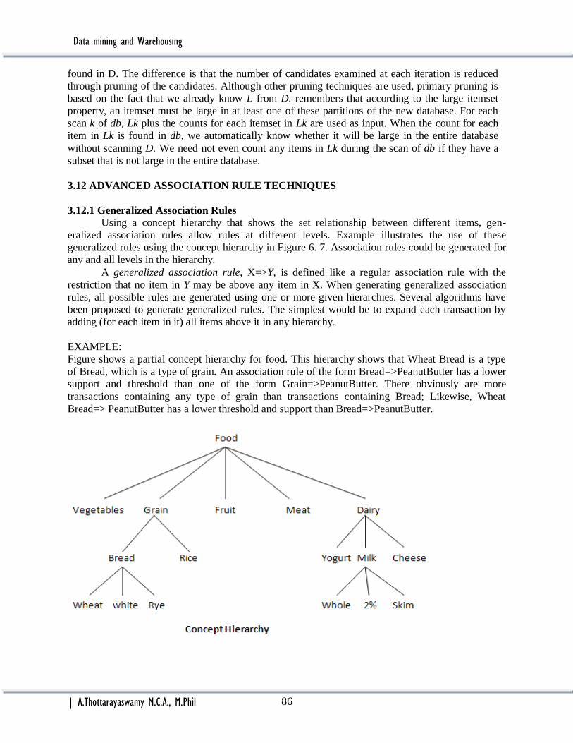
Data mining and Warehousing
| A.Thottarayaswamy M.C.A., M.Phil 86
found in D. The difference is that the number of candidates examined at each iteration is reduced
through pruning of the candidates. Although other pruning techniques are used, primary pruning is
based on the fact that we already know L from D. remembers that according to the large itemset
property, an itemset must be large in at least one of these partitions of the new database. For each
scan k of db, Lk plus the counts for each itemset in Lk are used as input. When the count for each
item in Lk is found in db, we automatically know whether it will be large in the entire database
without scanning D. We need not even count any items in Lk during the scan of db if they have a
subset that is not large in the entire database.
3.12 ADVANCED ASSOCIATION RULE TECHNIQUES
3.12.1 Generalized Association Rules
Using a concept hierarchy that shows the set relationship between different items, gen-
eralized association rules allow rules at different levels. Example illustrates the use of these
generalized rules using the concept hierarchy in Figure 6. 7. Association rules could be generated for
any and all levels in the hierarchy.
A generalized association rule, X=>Y, is defined like a regular association rule with the
restriction that no item in Y may be above any item in X. When generating generalized association
rules, all possible rules are generated using one or more given hierarchies. Several algorithms have
been proposed to generate generalized rules. The simplest would be to expand each transaction by
adding (for each item in it) all items above it in any hierarchy.
EXAMPLE:
Figure shows a partial concept hierarchy for food. This hierarchy shows that Wheat Bread is a type
of Bread, which is a type of grain. An association rule of the form Bread=>PeanutButter has a lower
support and threshold than one of the form Grain=>PeanutButter. There obviously are more
transactions containing any type of grain than transactions containing Bread; Likewise, Wheat
Bread=> PeanutButter has a lower threshold and support than Bread=>PeanutButter.
Data mining and Warehousing
| A.Thottarayaswamy M.C.A., M.Phil 87
3.12.2 Multiple-Level Association Rules
A variation of generalized rules are multiple-level association rules. With multiple-level
rules, itemsets may occur from any level in the hierarchy. Using a variation of the Apriori algorithm,
the concept hierarchy is traversed in a top-down manner and large itemsets are generated. When
large itemsets are found at level i, large itemsets are generated for level i + 1. Large k-itemsets at one
level in the concept hierarchy are used as candidates to generate large k-itemsets for children at the
next level.
Modification to the basic association rule ideas may be changed. We expect that there is more
support for itemsets occurring at higher levels in the concept hierarchy. Thus, the minimum support
required for association rules may vary based on level in the hierarchy. We would expect that the
frequency of itemsets at higher levels is much greater than the frequency of itemsets at lower levels.
Thus, for the reduced minimum support concept, the following rules apply:
The minimum support for all nodes in the hierarchy at the same level is identical.
If αi is the minimum support for level i in the hierarchy and αi-l is the minimum support for
level i-I, then αi -1 > αt;.
3.12.3 Quantitative Association Rules
The association rule algorithms discussed so far assume that the data are categorical. A
quantitative association rule is one that involves categorical and quantitative data. An example of a
quantitative rule is:
A customer buys wine for between $30 and $50 a bottle=> she also buys caviar.
This differs from a traditional association rule such as:
A customer buys wine=> she also buys caviar.
The cost quantity has been divided into an interval (much as was done when we looked at
handling numeric data in clustering and classification). In these cases, the items are not simple
literals. For example, instead of having the items {Bread, Jelly}, we might have the items
{(Bread:[0.. .1]), (Bread:(l... 2]), (Bread: (2 ... ∞)), (Jelly: [0..., 1.5]), (Jelly:(1.5.. .,3]), (Jelly:(3.. .
∞))}. The basic approach to finding quantitative association rules is found in Algorithm. Here we
show the Apriori algorithm being used to generate the large itemsets, but any such algorithm could
be used. ALGORITHM: Input:
I //Itemsets
P1, P2, … , PP // Processors
D = Dl, D2 , . . . ,DP;
s //Support
Output:
L //Large itemsets
Quantitative association rule algorithm:
for each Ij € I do / /Partition items.
if Ij is to be partitioned, then determine number of partitions;
map attribute values into new partitions creating new items; replace Ij in I with the new
items Ij1,… , Ijm;
Apriori(I, D, s);

Data mining and Warehousing
| A.Thottarayaswamy M.C.A., M.Phil 88
3.12.4 Using Multiple Minimum Supports:
When looking at large databases with many types of data, using one minimum support value
can be a problem. Different items behave differently. It certainly is easier to obtain a given support
threshold with an attribute that has only two values than it is with an attribute that has hundreds of
values. It might be more meaningful to find a rule of the form
SkimMilk WheatBread
With a support of 3% than it is to find
Milk Bread
with a support of 6%. Thus, having only one support value for all association rules may not
work well. Some useful rules could be missed. This is particularly of interest when looking at
generalized association rules, but it may arise in other situations as well. Think of generating
association rules from a non-market basket database. As was seen with quantitative rules, we may
partition attribute values into ranges. Partitions that have a small number of values obviously will
produce lower supports than those with a large number of values. If a larger support is used, we
might miss out on generating meaningful association rules.
This problem is called the rare item problem. If the minimum support is too high, then rules
involving items that rarely occur will not be generated. If it is set too low, then too many rules may
be generated, many of which (particularly for the frequently occurring items) are not important.
Different approaches have been proposed to handle this. One approach is to partition the data based
on support and generate association rules for each partition separately. Alternatively, we could
group rare items together and generate association rules for these groupings. A more recent
approach to handling this problem is to combine clustering and association rules. First we cluster
the data together based on some clustering criteria, and then we generate rules for each cluster
separately. This is a generalization of the partitioning of the data solution.
One approach, MISapriori, allows a different support threshold to be indicated for each item.
Here MIS stands for minimum item support. The minimum support for a rule is the minimum of all
the minimum supports for each item in the rule. An interesting problem occurs when multiple
minimum supports are used. The minimum support requirement for an itemset may be met even
though it is not met for some of its subsets. This seems to violate the large itemset property.
Example, which is adapted from [LHM99], illustrates this. A variation of the downward closure
property, called the sorted downward closure property, is satisfied and used for the MISapriori
algorithm. First the items are sorted in ascending MIS value. Then the candidate generation at scan
2 looks only at adding to a large item any item following it (larger than or equal to MIS value) in
the sorted order.
EXAMPLE:
Suppose we have three items, {A, B, C}, with minimum supports MIS(A) = 20%, MIS(B) = 3%,
and MIS(C) = 4%. Because the support for A is so large, it may be small, while both AB and AC
may be large because the required support for AB min(MIS(A), MIS (B) = 3% and
AC = min(MIS(A), MIS (C)) = 4%.
3.12.5 Correlation Rules
A correlation rule is defined as a set of itemsets that are correlated. The motivation for
developing these correlation rules is that negative correlations may be useful. Example, which
illustrates this concept. In this example even though the probability of purchasing two items together
seems high, it is much higher if each item is purchased without the other item. Correlation satisfies
upward closure in the itemset lattice. Thus, if a set is correlated, so is every superset of it.

Data mining and Warehousing
| A.Thottarayaswamy M.C.A., M.Phil 89
EXAMPLE:
Suppose there are two items, {A, B} where A B has a support of 15% and a confidence of
60%. Because these values are high, a typical association rule algorithm probably would deduce this
to be a valuable rule. However, if the probability to purchase item B is 70%, then we see that the
probability of purchasing B has actually gone down presumably because A was purchased. Thus,
there appears to be a negative correlation between buying A and buying B. The correlation can be
expressed as
Correlation (AB) = P(A, B) / P(A) P(B)
Which in this case is: 0.15 / 0.25x0.7= 0.857. Because this correlation value is lower than I, it
indicates a negative correlation between A and B.
3.13 MEASURING THE QUALITY OF RULES
Support and confidence are the normal methods used to measure the quality of an association
rule:
S(AB) = P(A, B) and α (AB) = P(B | A)
However, there are some problems associated with these metrics. For example, confidence
totally ignores P(B). A rule may have a high support and confidence but may be an obvious rule. For
example, if someone purchases potato chips, there may be a high likelihood that he or she would also
buy a cola. This rule is not really of interest because it is not surprising. Various concepts such as
surprise and interest have been used to evaluate the quality or usefulness of rules. We briefly
examine some of these in this section.
With correlation rules, we saw that correlation may be used to measure the relationship between
items in a rule. This may also be expressed as the lift or interest
Interest (AB) = P(A, B) / P(A) P(B)
This measure takes into account both P(A) and P(B). A problem with this measure is that it is'
symmetric. Thus, there is no difference between the value for interest (AB) and the value for
interest(BA). As with lift, conviction takes into account both P(A) and P(B). From logic we know
that implication AB=⌐(A ^ ⌐B). A measure of the independence: the negation of implication, then,
is P(A, ⌐B) / P(A) P(⌐B) .To take into account the negation. The conviction measure inverts this
ratio. The formula for conviction is:
Conviction (AB) = P(A) P(⌐B) / P(A, ⌐B)
Conviction has a value of I if A and B are not related. Rules that always hold have a value of 00.
The usefulness of discovered association rules may be tied to the amount of surprise
associated with the rules or how they deviate from previously known rules. Here surprise is a
measure of the changes of correlations between items over time. For example, if you are aware that
beer and pretzels are often purchased together, it would be a surprise if this relationship actually
lowered significantly. Thus, this rule beerpretzel would be of interest even if the confidence
decreased.
Another technique to measure the significance of rules by using the chi squared test for
independence has been proposed. This significance test was proposed for use with correlation rules.
Unlike the support or confidence measurement, the chi squared significance test takes into account
both the presence and the absence of items in sets. Here it is used to measure how much an itemset
(potential correlation rule) count differs from the expected. The chi squared test is well understood
because it has been used in the statistics community for quite a while. Unlike support and confidence,

Data mining and Warehousing
| A.Thottarayaswamy M.C.A., M.Phil 90
where arbitrary values must be chosen to determine which rules are of interest, the chi squared values
are well understood with existing tables that show the critical values to be used to determine
relationships between items.
The chi squared statistic can be calculated in the following manner. Suppose the set of items is
I = {I1, I2 ..., Im}. Because we are interested in both the occurrence and the nonoccurrence of an
item, a transaction tj can be viewed as
tj € {I1, ⌐I1} X … X {Im, ⌐Im}.
Contingency Table:
which is called a contingency table, shows the distribution
of the data In Example 6.9 assuming that tlie sample has
100 items in it. From this we find
E[AB] = 17.5, E[A ⌐B] = 7.5, E[⌐A B] = 52.5, E[⌐A ⌐B]
= 22.5, using these values we calculate X2 for this example as
X2 = (15-17.5)2 / 17.5 + (10-7.5)2 / 7.5 + (55-52.5)2 / 52.5 + (20-22.5)2 / 22.5 = 1.587
If all values were independent, then the chi squared statistic should be O. A chi squared table (found
in most statistics books) can be examined to interpret this value. Examining a table of critical values
for the chi squared statistic, we see that a chi squared value less than 3.84 indicates that we should
not reject the independent assumption. This is done with 95% confidence. Thus, even though there
appears to be a negative correlation between A and B, it is not statistically significant.
B B Total
A 15 10 25
A 55 20 75
Total 70 30 100
Data mining and Warehousing
| A.Thottarayaswamy M.C.A., M.Phil 91
4. DATA WAREHOUSING
An Introduction
4.1 Characteristics of a Data Warehouse:
A data warehouse is a repository of subjectively selected and adapted operational data, which
can successfully answer any ad hoc, complex statistical or analytical queries. It is situated at the
center of a decision support system (DSS) of an organization. Data warehousing technology is
becoming essential for effective business intelligence, business strategy formulation and
implementation in globally competitive environment.
Data warehousing enables easy organization and maintenance of large data in addition to fast
retrieval and analysis in the manner and depth required from time to time.
Data classified into three categories:
1. Reference and transaction data
2. Derived data
3. Demoralized data
Reference and transaction data originates form operational (source) system and is normally
kept in a conventional database system. Derived data, is only derived from the reference and
transaction data, based on certain rules or computations. Demoralized data, which is the basis for
online analytical processing (OLAP) tools, is prepared periodically but directly based on detailed
reference (transaction) data.
4.2 Data Marts From a Data warehouse, data flows to various departments for their customized DSS usage.
Theses individual department components are called data marts, a data mart is a body of DSS data
for a department that has an architectural foundation of data warehouse. Data mart is a subset of a
data warehouse and is much more popular than data warehouse.
When the data warehouse in small, the analyst (of DSS) can easily customized, summarize
and analyze to draw analytical results relatively easily. The data becomes very large as it calls for
large amount of time. The processing load or overhead is also very limited in the case. Whereas, the
resource requirement are very restricted. The data mart is so attractive, because a data mart is a
natural outgrowth of a data warehouse. The detailed data is customized, sorted or summarized as it is
placed in the data mart.
UNIT 4 - Introduction
4.1 characteristics of a data warehouse
4.2 data marts
4.3 other aspects of data mart

Data mining and Warehousing
| A.Thottarayaswamy M.C.A., M.Phil 92
4.2.1 Types of data marts 1. Multidimensional (MDDB OLAP or MOLAP)
2. Relational (ROLAP)
Multidimensional (MDDB) data mart, the numeric data, which is basically
multidimensional in its original nature, can be sliced and diced in free fashion.
(i.e Free data modelling constraints) stored as basic tables in RDBMS, even though the data
inherently may be multidimensional, (i.e year-wise, region-wise, etc.) it in terms of tabular form of
data.
Relational OLAP data marts may contain both text and numeric data and supported by
RDBMS. These data marts are used for general purpose DSS analysis with many indices which
support for star schema. It can be analyzed either on ad hoc basis or on preconceived queries.
4.2.2 Loading a data marts The data mart is loaded with data form a data warehouse by means of a load program.
The considerations for a load program are:
Frequency and schedule – total or partial refreshment (addition).
Customization of data from the warehouse (selection).
Re-sequencing and merging of data.
Aggregation of data.
Summarization.
Efficiency (loading time optimization).
Integrity of data.
Data relationship and integrity of data domains.
Producing Meta data for describing the loading process.
4.2.3 Metadata for a data mart Metadata (data about data) describes the details (flow of data) about the data in a data
warehouse or in a data mart.
Components of metadata for given data warehouse or data mart:
Description of source of the data.
Description of customization that may have taken place as the data passes from data
warehouse into data mart.
Descriptive information about data mart (tables, attributes, relationship etc).
Definitions of all types.
The metadata of a data mart is created and updated form the load programs that move data form
data warehouse to data mart. The linkage and relationships between metadata of a data warehouse
and metadata of data mart have to be well established or well understood by the manager or analyst
using the metadata.
4.2.4 Data model for data mart A formal data model is required to be built for a large data mart which may also have some
processing involved. This processing can be repetitive or predictable. No data model is necessary for
ordinary or simple small data marts with no processing. For example the multidimensional data
model itself is a necessity for that DBMS.

Data mining and Warehousing
| A.Thottarayaswamy M.C.A., M.Phil 93
4.2.5 Maintenance of data mart Periodic maintenance of a data mart means loading, refreshing and purging the data in it.
Refreshing the data is performed in regular cycles as per the nature of frequency of data update. (ex.
Rainfall data)
To purging of data in a data mart, the data mart is read periodically and some (old) data is
selected for purging (edit) or removing. (ex. Depends on date, time)
4.2.6 Nature of data in a data mart
The data in a data mart can be of detailed level, summary level, ad hoc data (lot of
aggregations), preprocessed or prepared data.
4.2.7 Software components for a data mart
The software that can be found with a data mart includes:
DBMS,
Access and analysis software,
Software for automatic creation of data marts,
Purging and archival software,
Metadata management software, etc
The access and analysis software, which is the most unique for data warehousing application,
allows the end-user to search through the data mart to find and compute or derive the data required
by the user.
4.2.8 Tables in the data mart
A data mart may include:
Summary table,
Detailed tables,
Reference table,
Historical tables,
Analytical (spreadsheet) tables, etc
As the data grows, the backlog back-up may be kept as „library‟, which can also serve the
purpose of a quick reference for a survey of available data, as and when required.
The data is kept in the tables in the form of star joins on normalized tables. When the data in
not large, relational tables are adequate.
4.3 Other aspects of data mart
4.3.1 External data
First: if required to be used by more than one data mart, shall be best placed in the data
warehouse itself and then subsequently be moved to the data marts required. This will avoid
redundancy and duplication in procurement of external data.
Secondly: when a particular external data is acquired, its „pedigree‟ or descriptive details in
addition to the data are also required to be stored.
These details includes the source of external data –

Data mining and Warehousing
| A.Thottarayaswamy M.C.A., M.Phil 94
Size and data of acquisition of the external data,
Editing and filtering criteria applied to the external data, etc.
4.3.2 Reference data
The reference data table, stored in addition to basic data in the data mart help and enables the
end-user of the data mart to relate the data to its expanded version. The end-user can operate the data
in short hand, if desired. The data mart itself will store and manage its own reference tables. When
reference tables are stored and managed in DSS environment, there is a need to manage their
contents over time.
4.3.3 Performance issues
The performance considerations in DSS environment are very much different from those in
OLAP environment. The response time issues are totally different, there is no need for real time or
online response as is required in the case of OLTP systems.
Good performance can be achieved in a data mart environment by:
Extensive use of indexes, Using star joins, Limiting the volume of the data,
Creating arrays of data, creating profile records, Creating pre-joined tables, etc.
4.3.4 Monitoring requirements for a data mart
Periodic monitoring is required on data mart behavior. Monitoring mainly relates data usage
to data content tracking.
Data usage tracking has queries on the data mart such as;
What data is being accessed?
Which user are active?
What is the quantity of data accessed?
What are the usage timings?
The data content tracking includes the following queries:
What are the actual contents of the data mart?
What is the best way of accessing?
Is there any bad data in the data mart?
How and how much of the data is growing?
4.3.5 Security in a data mart
When there is secretive information in the data mart it needs to be secured well. Typically,
secretive information includes financial information, medical records and human resources
information, etc.
The data mart administrator should make necessary security arrangements such as:
Firewalls, Log on/off security, Application base security, DBMS security, Encryption and
decryption.
The information cost of security depends upon its exclusiveness.

Data mining and Warehousing
| A.Thottarayaswamy M.C.A., M.Phil 95
ONLINE ANALYTICAL PROCESSING
4.4 Introduction
Online analytical processing (OLAP) systems, contrary to the regular, conventional online
transaction processing (OLTP) systems, are capable of analyzing online a large number of past
transactions or large number of data records and summarize them on the fly.
Any multidimensional data as spreadsheet, cannot be processed by conventional SQL type
DBMS. As such, multidimensional query on such a database will explode into a large number of
complex SQL statements each of which may involve full table scan, multiple joins, aggregation,
sorting and also large temporary table space for storing temporary results.
4.5 OLTP and OLAP systems
OLTP OLAP
1. Only current data available (old
data is replaced by current data
by updating)
2. Short transactions (single
granularity or more)
3. Online update/insert/delete
transactions
4. High volume of transactions in a
given period
5. Concurrency control and
transaction recovery
6. Largely online ad hoc queries,
requiring low level of indexing
1. Both current and historic data
available (current is appended to
historic data)
2. Log database transactions
3. Batch update/insert/delete
transactions
4. Low volume transactions, periodic
refreshing
5. No concurrent transactions and
therefore no recovery upon failures
required
6. Largely pre-determined queries
requiring high level of indexing
A very popular and early approach for achieving analytical processing is star schema or
collection model. This involves denormalization of data followed by integration as shown in the
three-tier architecture.
UNIT 4 - OLAP
4.4 Introduction
4.5 OLTP & OLAP systems
4.6 Data modelling- star schema for multidimensional view
4.7 Data modelling- multifact star schema or snow flake schema
4.8 OLAP TOOLS
4.9 State of the market
4.10 OLAP TOOLS and the internet

Data mining and Warehousing
| A.Thottarayaswamy M.C.A., M.Phil 96
Operational level
Extraction
Transformation
Transaction data
User‟s view Analytical level
Fig . Three-tier architecture of data warehousing environment.
The data extracted from individual data sets is accumulated into a data warehouse after
transformation. All tables are required to be denormalized and stored in a star or collection table that
is more in line with user‟s understanding of the data as shown in fig.
Cross-referencing data sets
Order transactions identified by parts, customers or regions
Fig. Implementing star schema approach through pre-joining of tables.
Source A
Part A
Source B
Part B
Source C
Part C
A B C
A B
Part
s Customer Order
s
Region
s
A collection of integrated data
(parts, customers, orders, regions)
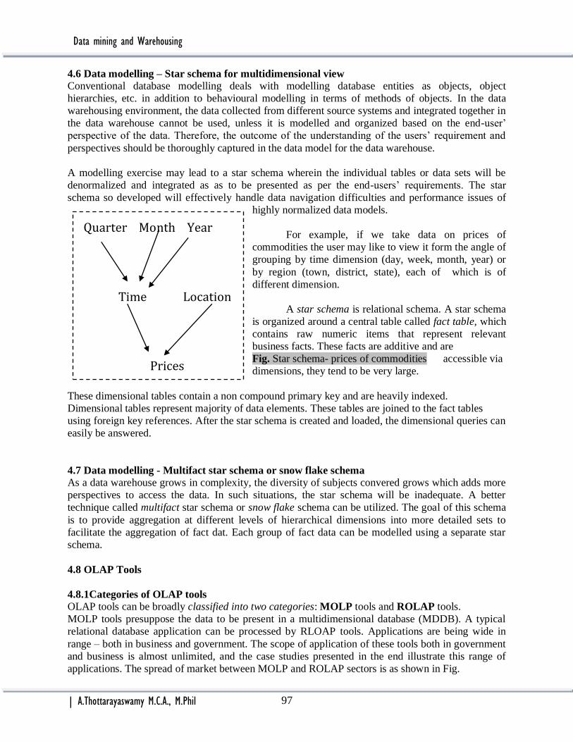
Data mining and Warehousing
| A.Thottarayaswamy M.C.A., M.Phil 97
4.6 Data modelling – Star schema for multidimensional view
Conventional database modelling deals with modelling database entities as objects, object
hierarchies, etc. in addition to behavioural modelling in terms of methods of objects. In the data
warehousing environment, the data collected from different source systems and integrated together in
the data warehouse cannot be used, unless it is modelled and organized based on the end-user‟
perspective of the data. Therefore, the outcome of the understanding of the users‟ requirement and
perspectives should be thoroughly captured in the data model for the data warehouse.
A modelling exercise may lead to a star schema wherein the individual tables or data sets will be
denormalized and integrated as as to be presented as per the end-users‟ requirements. The star
schema so developed will effectively handle data navigation difficulties and performance issues of
highly normalized data models.
For example, if we take data on prices of
commodities the user may like to view it form the angle of
grouping by time dimension (day, week, month, year) or
by region (town, district, state), each of which is of
different dimension.
A star schema is relational schema. A star schema
is organized around a central table called fact table, which
contains raw numeric items that represent relevant
business facts. These facts are additive and are
Fig. Star schema- prices of commodities accessible via
dimensions, they tend to be very large.
These dimensional tables contain a non compound primary key and are heavily indexed.
Dimensional tables represent majority of data elements. These tables are joined to the fact tables
using foreign key references. After the star schema is created and loaded, the dimensional queries can
easily be answered.
4.7 Data modelling - Multifact star schema or snow flake schema
As a data warehouse grows in complexity, the diversity of subjects convered grows which adds more
perspectives to access the data. In such situations, the star schema will be inadequate. A better
technique called multifact star schema or snow flake schema can be utilized. The goal of this schema
is to provide aggregation at different levels of hierarchical dimensions into more detailed sets to
facilitate the aggregation of fact dat. Each group of fact data can be modelled using a separate star
schema.
4.8 OLAP Tools
4.8.1Categories of OLAP tools
OLAP tools can be broadly classified into two categories: MOLP tools and ROLAP tools.
MOLP tools presuppose the data to be present in a multidimensional database (MDDB). A typical
relational database application can be processed by RLOAP tools. Applications are being wide in
range – both in business and government. The scope of application of these tools both in government
and business is almost unlimited, and the case studies presented in the end illustrate this range of
applications. The spread of market between MOLP and ROLAP sectors is as shown in Fig.
Quarter Month Year
Time Location
Prices

Data mining and Warehousing
| A.Thottarayaswamy M.C.A., M.Phil 98
Application
Complexity
Application performance
Fig. OLAP comparison. The area of circles indicate the data size.
- MOLAP
Info
Load request
SQL
Result
Result set
Set
Fig MOLAP architecture.
MOLAP based products organize, navigate and analyze data typically in an aggregated
from. They require tight coupling with the applications and they depend upon a multidimensional
database (MDDB) system. Efficient implementations store the data in a way similar to the form in
which it is utilized by using improved storage techniques so as to minimize storage. Many efficient
techniques are used as sparse data storage management on disk so as to improve the response time.
Some OLAP tools, as Pilot products introduce time also as an additional dimension for analysis,
ROLAP
MOLAP
Database server
MOLAP server
Metadata
Request
Processing
Front end tool

Data mining and Warehousing
| A.Thottarayaswamy M.C.A., M.Phil 99
thereby enabling time series. Some products as Oracle Express Server introduce strong analytical
capabilities into the database itself.
Applications requiring iterative and comprehensive time series analysis of trends are
well suited for MOLAP technology. Examples include Arbor Software‟s Essbase, Oracle‟s express
server, pilot software‟s lightship server, sinper‟s TM/1, Planning science‟s gentium and kenan
technology‟s multiway.
- ROLAP
Info
SQL Request
Result
set
result
set
Fig ROLAP architecture
Relational OLAP is the latest and fastest growing OLAP technology segment in the market. Many
vendors have entered the fray in this direction. By supporting a dictionary layer of meta data, the
RDBMS products have bypassed any requirement for creating a static, multidimensional data
structure as shown in above fig.
Some products in this segment have supported strong SQL engines to support the complexity of
multidimensional analysis. This includes creating multiple SQL statements to handle user requests,
being „RDBMS aware‟ and also being capable of generating the SQL statement based on optimizer
of the DBMS engine. Vendors of ROLAP tools and RDBMS products are now eager to provide
multidimensional persistent structures with facilities to assist in the administrations of these
structures. Notable among vendors of such products are Microstrategy, Platinum/Prodea Software
(Beacon), Information Advantage (AxSys), Informx/Stanford Technology Group (Metacube) and
SyBASE.
Database server
MOLAP server
Metadata
Request
Processing
Front end tool

Data mining and Warehousing
| A.Thottarayaswamy M.C.A., M.Phil 100
4.8.2 Managed query environment (MQE) Recent trend of OLAP is to enable capability for users to perform limited analysis directly against
RDBMS products or by bringing in an intermediate limited MOLAP server (see fig.)
SQL query
Result set OR
Load info
request
SQL
Result set result set
Fig Hybrid/MQE architecture.
Some vendors‟ products have been able to provide ad hoc query as data cube and slice and dice
analysis capabilities. This is achieved by first developing a query to select data from the DBMS,
which then delivers requested data to the desktop system where it is placed into a data cube. This
data cube can be locally stored in the desktop and also manipulated there so as to reduce the
overhead required to create the structure each time the query is executed. Once the data is placed in
the data cube the user can locally perform multidimensional analysis and also slice, dice and pivot
operations on it. In another approach, these tools can work with MOLAP servers, the data from
RDBMS can first go to MOLAP server and then to the desktop.
The ease of operation, administration and installation of such products makes them particularly
attractive to users who are familiar with simple RDBMS usage and environment.
4.9 State of the market
4.9.1 Overview of the stat of the international market
Basically OLAP tools provide a more intuitive and analytical way to view corporate or
organizational data. These tools aggregate data along common subjects of business or dimensions
and then let users navigate through the hierarchies and dimensions with the click of a mouse. Users
can drill down, across, or up across levels in each dimension or pivot and swap out dimensions to
change their view of the data. All this can be achieved by various OLAP tools in the international
market. Such free manipulation of data provides insight into data, usually not possible by any other
means (Kimball, 1996).
Database server
RDBMS
MOLAP server
Front end tool

Data mining and Warehousing
| A.Thottarayaswamy M.C.A., M.Phil 101
Some tools, such as Arbor software corp.‟s Essbase and Oracle‟s express, preaggregate data into
special multidimensional databases. Other tools work directly against relational data and aggregate
data on the fly, such as Microstrategy Inc.‟s DSS Agent or Information Advantage Inc.‟s
DecisionSuite.
4.9.2 Cognos powerplay
Cognos powerplay is an open OLAP solution that can interface and interoperate with a wide
variety of third-party software tools, databases and applications. The analytical data used by
powerplay is stored in multidimensional data sets called PowerCubes. Cognos‟ client/server
architecture allows for the powercubes to be stored on the Cognos universal client or on server.
Cognos powerplay client offers:
*Support for enterprise-size data sets (powercubes) of 20+ million records, 100,000
categories and 100 measures
*A drill-through capability for queries from Cognos impromptu powerful 3-D charting
capabilities with background and rotation control for advanced users
*Scatter charts that let users show data across two measures, allowing easy compassion of
budget to actual values
*Linked displays that give users multiple views of the same data in report
*Full support for OLE2 automation, as both a client and a server
*Formatting features for financial reports: brackets for negative numbers, single and double
underlining, and reverse sign for expenses
*Faster and easier ranking of data
*A home button that automatically resets the dimension line to the top level
*Unlimited undo levels and customizable toolbar
*Powerplay reports, word processing, spreadsheet, presentation documents
*A 32 bit architecture for windows NT, windows 95/98
*Advanced security control by dimension, category and measure on the client, the sever both
In powerplay administrator database edition, the administrator would continue to model the
cube and run the population of the cube process (called transform) on the client platform. The
advantage is that data from multiple sources can now be used to generate a pointercube can be inside
a relational database. An administrator uses client transformer to create a model and moves it to the
UNIX server using the supplied software component called Powergrid. The server transformer, once
triggered, will create the powercube, and the only prerequisite is that all data sources be accessible.
4.9.3 IBI focus fusion Focus fusion from Information Builders Inc.(IBI) is a multidimensional database technology
for OLAP and data warehousing. It is designed to address business applications that require
multidimensional analysis of detail product data. Focus fusion complements cactus and EDA/SQL
middleware software to provide a multifaceted data warehouse solution.
Designed specifically for deployment of business intelligence applications in data warehouse
environments, fusion provides:
* Fast query and reporting – advanced indexing, parallel query, roll-up facilities, reports,
queries and analyses, complete data warehouse solutions
*Graphics based administration facilities
*Integrated copy management facilities
*Span reporting, query, DSS
Data mining and Warehousing
| A.Thottarayaswamy M.C.A., M.Phil 102
*Supports ANSI SQL, ODBC, HTTP via EDA/SQL
*Three – tiered reporting architecture
*Access to pre calculated summaries (roll-up)
*Support for parallel computing environment
And includes the following components:
*Fusion/DBserver: High performance, client/server, parallel enabled, scalable
multidimensional DBMS.
*Fusion/Administrator: Comprehensive GUI based administration utility that provides visual
schema definition and bulk load of fusion database
*Fusion/PDQ: Parallel data query for fusion/DBserver exploits symmetric multiprocessor
(SMP) hardware for fast query execution and parallel loads
*EDA/Link: Fusion‟s client component support standard APIs, including ODBC and ANSI
SQL. Also provides access to fusion from any desktop
*EDA/Weblink: Fusion open browser client that support netscape, mosaic, IE
*Enterprise copy manager for fusion: Fully automated assembly, transformation,
summarization, and load of enterprise data from any source
*EDA Gateways: Remote data access gateways that provide transparent, live drill through
capabilities from fusion/DBserver to production databases
4.9.4 Pilot software Pilot Software offers the Pilot Decision Support of tools from a high speed
multidimensional database (MOLAP), data warehouse integration (ROLAP), data mining, and a
diverse set of customizable business applications targeted after sales
and marketing professionals.
The following products are at the core of Pilot. Software's offering:
Pilot Analysis Server. A full-function multidimensional database with high speed consolidation,
graphical user interface (Pilot Model Builder), and expert-level interface. The latest version includes
relational integration of the multidimensional model with relational data stores, thus allowing the
user the choice between high-speed access of a multidimensional database or on the-fly (ROLAP)
access of detail data stored directly in the data warehouse or data mart.
Pilot Link. A database connectivity tool that includes ODBC connectivity and high-speed
connectivity via specialized drivers to the most popular relational database platforms. A graphical
user interface allows the user seamless and easy access to a wide variety of distributed databases.
Pilot Designer. An application design environment specifically created to Enable rapid
development of OLAP applications.
Pilot Desktop. A collection of applications that allow the end-user easy navigation and
visualization of the multidimensional database.
Pilot Sales and Marketing Analysis Library. A collection of sophisticated applications designed
for the sales and marketing business end-user (including 80/20 Pareto analysis, time-based ranking,
BCG quadrant analysis, trend line and statistical forecasting). The applications can be modified and
tailored to meet individual needs for particular customers.
Pilot Discovery Server. A predictive data mining tool that embeds directly into the relational
database and does not require the user to copy or transform the data. The data mining results are
stored with metadata into the data warehouse as a predictive segmentation and are embedded into the
graphical user interface called Pilot Discovery Server Launch, which helps building data mining
models.

Data mining and Warehousing
| A.Thottarayaswamy M.C.A., M.Phil 103
Pilot Internet Publisher. A tool that easily allows users to access their Pilot multidimensional
database via browsers on the Internet or Intranets.
Some of the distinguishing features of Pilot's product offering include the overall complete
solution from powerful OLAP engine and data mining engine to their customizable business
applications. Within their OLAP offering, some of the key features of Pilot's products are as under:
Time intelligence. The Pilot Analysis Server has a number of features to support time as a
special dimension. Among these are the ability to process data on the fly to convert the native
periodicity (e.g. the data collected weekly) to the periodicity preferred by the customer viewing the
data (e.g. view the data monthly). This feature is accomplished via special optimized structures
within the multidimensional database.
Embedded data mining. The Pilot Analysis Server is the first product to integrate predictive
data mining with the multidimensional database model. This allows the user to benefit not only from
the predictive power of data mining but also from the descriptive and analytical power of
multidimensional navigation.
Multidimensional database compres$ion. In addition to the compression of sparsity, Pilot
Analysis Server also has special code for compressing data values over time. A new feature called a
'dynamic dimension' allows some dimensions to be calculated on the fly when they are attributes of
an existing dimension. This allows the database to be much smaller and still provide fast access.
Dynamic variables which are also calculated on the fly are also available to further decrease the total
size of the database and thus decrease the time for consolidation of the database.
Relational integration. Pilot allows for a seamless integration of both MOLAP and ROLAP
to provide the user with either the speed of MOLAP or the more space-efficient ROLAP. The users
interface with the system by defining the multidimensional model or view that they prefer, and the
system self-optimizes the queries.
4.9.5 Arbor Essbase Web
Essbase is one of the most ambitious of the early Web products. It includes not only OLAP
manipulations, such as drill up down and across, pivot, slice and dice; and fixed dynamic reporting
but also data entry, including full multi-user concurrent write capabilities-a feature that differentiates
it from the others.
Arbor sells Essbase only as a server, it does not have a client package. The Web product does
not replace administrative and development modules; only user can access it for query and update.
4.9.6 Information Advantage Web OLAP
Information Advantage uses a server-centric message architecture, which is composed of a
powerful analytical engine that generates SQL. It also pulls data from relational databases,
manipulates the results and transfers the results to a client.
Since all the intelligence of the product is in the server implementing Web OLAP to provide a
Web-based client is straightforward, the architecture of Information Advantage's Web product is
similar to that of Essbase with a Web gateway between the Web server and the analytical engine.
Although in this case, data store and an analytical engine are separate, Essbase is both data store and
analytical engine.

Data mining and Warehousing
| A.Thottarayaswamy M.C.A., M.Phil 104
4.9.7 Microstrategy DSS Web
Microstrategy's DSS Agent was originally a Windows-only tool, but now it is also OLAP tool to
have a Web-access product. DSS along with DSS server relational OLAP server-DSS architect data
modelling tool, and DSS executive design tool for building Executive Information Systems-generates
SQL dynamically and relies on the relational database server to perform complex analysis, rather
than creating a 'cube' like most of the other tools. By inserting a Web gateway between the Web
server and the DSS server engine, Microstrategy was able to replace the interactive DSS agent front-
end with a Web browser, which passes requests to the DSS server's API.
4.9.8 Brio Technology
Brio offers a suite of products called Brio. web. warehouse. This suite implements several
of the approaches listed above for deploying decision support OLAP applications on the Web. The
key to Brio's strategy are new server components called Brio.quickview and Brio.insight which can
off load processing from the clients and thus enable users to access Brio reports via Web browsers.
On the client side, Brio uses plug-ins to give users viewing and manipulation capabilities. For these
and other reasons, the Web is a perfect medium for decision support.
The general features of the Web-enabled data access are as under:
The first-generation Web sites used a static distribution model, in which clients access static
HTML pages via Web browsers. In this model, the decision support reports are stored as HTML
documents and are delivered to users on request. Clearly, this model has some serious deficiencies,
including. inability to provide Web clients with dynamic updates and interactive analytical
capabilities such as drill-down.
The second-generation Web sites support interactive and dynamic database by utilizing a
multi tiered architecture in which a Web client submits a query in the form of HTML-encoded
request to a Web server, which in turn transforms the request for structured data into a Common
Gateway Interface (CGI) script, or a script written to a proprietary Web-server API (Le.
Netscape server API, or NSAPI). The gateway submits SQL queries to the database, receives the
results, translates them into HTML and sends the pages to the requester. Requests for the
unstructured data (e.g. images, other HTML documents, etc.) can be sent directly to the
unstructured data store, pre-calculated MOLAP storage or directly in the relational data store
depending on the usage pattern and the time/space trade-off preferences of the end user.
4.10 OLAF TOOLS AND TUE INTERNET The Web technologies indeed are the natural choice for adaptation for data warehousing (and vice
versa). The internet is virtually a free (or a very low cost) resource which provides a universal
connectivity within and between companies and also individuals.
Some of the web facilities are as under:
The Web eases complex administrative tasks of managing distributed environments.
The Web allows companies to store and manage both data and applications on servers that
can be centrally managed and updated, thus eliminating problems with software and data accuracy.
The emerging third-generation Web sites replace HTML gateways with Web based
application servers. These servers can download Java applets or ActiveX applications that execute on
clients, or interact with corresponding applets running on servers-servlets. The third-generation Web
servers provide users with all the capabilities of existing decision-support applications without
requiring them to load any client software except a Web browser.
Data mining and Warehousing
| A.Thottarayaswamy M.C.A., M.Phil 105
Not surprisingly, vendors of decision support applications, especially query, reporting and
OLAP tools, are rapidly converting their tools to work on the Web. Vendor approaches for deploying
tools on the Web include the following:
HTML publishing. This approach involves transforming an output of a query into the HTML
page that can be downloaded into browser. This approach does not support interactive access to data
or reports.
Helper applications. In this approach, a tool is configured as a helper application that resides
within a browser. This is the case of a 'fat' (or thick) client, in which, once the data is downloaded,
users can take advantage of all capabilities of the tool to analyze data. However, maintaining these
helper applications becomes another task for system administrators.
Plug-ins. A variation on the previous approach, plug-ins are helper applications that are
downloaded from the server prior to their initial use. Since the plug-in are downloaded from the
server, their normal administration and installation tasks are significantly reduced. However,
typically, plug-ins are browser-specific and may not run on all platforms or with all browsers. Also,
as browsers get updated, these plug-ins may have to be upgraded as well, creating additional
administration workload.
Server-centric components. In this approach, the vendor rebuilds a desktop tool as a server
component, or creates a new server component that can be integrated with the Web via a Web
gateway (e.g. CGI or NSAPI scripts).
Java and ActiveX applications .This approach is for a vendor to redevelop all or portions of
its tool in Java or ActiveX. The result is a true 'thin' client model. Despite some disadvantages, this
approach appears to be one of the most promising and flexible.
The following are some of the Web-based tools:
Arbor Essbase Web. This tool offers features as drilling up, down, across; slice and dice and
dynamic reporting, all for OLAP. It also offers data entry, including full multi-user concurrent write
capabilities. Arbor Essbase is only a server product, no client package exists, thus protecting its own
desktop (stand alone) client version market. The Web product does not replace administrative and
development modules but it replaces only user access for query and update.
Information Advantage Web OLAP. This product uses a server centric messaging
architecture, composed of a powerful analytic engine which generates SQL for the retrieval from
relational database, manipulate the results and transfer the results into a client. Since it is all server-
centric capability, implementing Web OLAP to provide web-based client is easy and simple. This
architecture is similar to the one of Essbase with a Web gateway between Web server and analytic
engine, even though the data store and the engine are separate (as against \ Essbase which is both a
data store and analytic engine).
Microstrategy DSS Web. The flagship product DSS Agent form Microstrategy, originally a
Window tool, is now available on all platforms (as NT) and also on the Web. DSS Agent, along with
the complement product-DSS server relational OLAP server, DSS Architect data-modelling tool, the
DSS Executive design tool for building executive information system (EIS) , generates SQL
automatically and dynamically. It depends on the RDBMS server for performing complex analysis,
instead of creating a multidimensional 'Cube'. Then it is offering ROLAP (relational OLAP) and not
MOLAP (multidimensional OLAP). By inserting a Web gateway between the Web server and DSS
server engine, Microstrategy is replacing the interactive DSS Agent front-end with a web browser
which passes through it in terms of requests to DSS server API.
Brio technology. Brio released 'brio. web. warehouse suite of products in the end of 1998.
Most of the Web OLAP approaches described earlier are available in this suite. A new server
component called 'brio.query.server' works in tandem with Brio Enterprise Web-clients
'brio.quickview' and 'brio.insight' and enable Web access by browsers.

Data mining and Warehousing
| A.Thottarayaswamy M.C.A., M.Phil 106
DEVELOPING A DATA WAREHOUSE
5.1 Why and how to build a data warehouse?
Changes are taking place in the world continuously in all forms of activity. From a business
perspective, the quest for survival in a globally competitive environment has become extremely
demanding for all.
As discussed in Unit 4, in this scenario, business strategy requires answers to questions in
business policy and future strategy. This means that the decisions are required to be taken quickly
and correctly using all the available data. As the data size increases continuously, doubling every 18
months, the speed requirements for processing this data so as to comprehend the meaning of this data
are also required to be increased significantly. Competition also adds pressure on this situation and
herein business intelligence becomes the foundation for successful business strategy (Bracket, 1996).
Here the need for data warehousing technology arises, in terms of the ability to organize,
maintain large data and also be able to analyze in a few seconds in the manner and depth as required.
(Inmon and Hackathorn,1994). Why did the conventional information systems not succeed in
meeting these requirements? Actually the conventional information systems and data warehousing
tackle two different activity domains-OLTP and OLAP. (as discussed in Unit 4). These domains are
not at all competitive with each other; they deal with two different problem domain requirements.
Further, as the technology upgrades, the CPU time and disk space are growing larger and are
becoming cheaper with time. Similarly, network bandwidths are increasing and becoming cheaper
day by day. Need for more and more heterogeneity and interoperability is increasingly being felt. In
this scenario, data warehousing emerges as a promising technology (Anahory and Murray, 1997).
In the following sections, we shall survey all the major issues involved in building a data
warehouse, such as approach, architectural strategy, design considerations, data content related
issues, meta-data, distribution of data, tools and performance considerations.
5.2 Data warehouse architectural strategies and organization issues
A data warehouse can be built either on a top-down or on a bottom-up approach. In other
words, one can define a global data warehouse for an entire organization and split it up into
individual data marts or sub data warehouses dedicated for individual departments. Alternatively
individual data marts can be built for each department and then they all get finally integrated into a
central data warehouse (Bischoff and Alexander, 1997).
The bottom-up approach is more realistic but the integration of individual data marts should
be made easier with advanced planning and preparation.
UNIT 5 - Introduction
5.1 Why and how to build a data warehouse
5.2 Data warehouse architectural strategies and organization issues
5.3 Design consideration
5.4 Data content
5.5 Metadata
5.6 Distribution of data
5.7 Tools for data warehousing
5.8 Performance considerations
5.9 Crucial decisions in designing a data warehouse.

Data mining and Warehousing
| A.Thottarayaswamy M.C.A., M.Phil 107
All organizations active in information systems area are fully conversant with the issues
relating to information systems implementation.- But the issues pertaining to data warehousing
activity are quite different and divergent from these ones. In building a data warehouse, the
organization has to make arrangements for information flow from various internal information
systems and databases as well as from internal sources of information. This requires close
involvement of the users in identifying the information requirements and identifying the sources of
the same from both internal and external data sources and information systems in time (Devlin,
1997).
5.3 Design consideration
The first and foremost design consideration is to be exhaustive and so to say holistic, i.e. to
exhaustively cover all possible data sources for exhaustively designing a data warehouse with all
possible components as part of a single complex system so as to effectively meet all possible user
requirements. Any failure in this regard may lead to a data warehouse design that is skewed towards
a particular requirement (missing other requirements) or a particular data source, missing some other
data sources or oriented towards a particular access tool, thereby limiting its usage and accessibility.
Web enablement may subsequently enhance the data accessibility and its usage.
There are three major issues that will be faced in data warehouse development:
heterogeneity of data sources requiring substantial efforts in data conversion and also in maintaining
timeliness and high-quality levels of data integrity, reliability and authenticity. Further, the data may
be quite old and historical. While old data of past is essential for a data warehouse, it should be
ensured that it will be relevant and useful in the data warehouse form. If any data is too old to be
relevant any more it may not be worthwhile to enter into the data warehouse. Another issue is the
tendency of the data warehouse to grow very large. Discrete decisions should be made by the
designer of the data warehouse in limiting the size of the warehouse by discretely dropping old data
and selecting appropriate data to be included into the warehouse.
The data warehouse design is distinctly different from regular OLTP based information
system design in many ways. Data warehouse design is business driven, i.e. it is based on specific
business goals to be achieved by the OLAP on the data warehouse. In the case of OLTP systems, the
design is driven by the existing information system concerned. Since data warehouse design is
business driven, it may never be fully completed as the users' business requirements and also data
sources keep changing. Keeping them in view the designer may be cautious in data warehouse design
so as to avoid the possible pitfalls.
5.4 Data content
In what way does the data content in the warehouse differ from OLTP system? It is normally
misunderstood that data warehouse contains lesser level of detailed data when compared to an OLTP
system which may be its source. This is incorrect. The level of detail of data in the data warehouse is
normally the same as that of the source OLTP system; only it may be in a different format. Typically,
a data warehouse contains detail level data. But the data is cleaned and transferred to fit in the data
warehouse model.
The cleaning up process removes the deficiencies and loopholes in the data. In addition, all
the aspects related to transaction processing also will be filtered off before putting into the
warehouse, as they are not relevant in OLAP applications of the warehouse.
The data model used in the data warehouse reflects the nature, content and structure of the
data in the data warehouse. The data model represents the framework of the organization and
structure of the data in the data warehouse (we have already discussed this issue in Unit 4). The data
model also identifies how the information is stored in the data warehouse. It identifies major subjects
and relationships of the model, including keys, attributes and attribute groupings.
Data mining and Warehousing
| A.Thottarayaswamy M.C.A., M.Phil 108
In addition to the data model, the designer should also be able to identify the querying
process on the warehouse. Due to their broad scope and powerful nature, queries can also determine
the data model. The data model should be optimized so as to meet high level query performance in
terms of broad scope and analytical intensity. In addition, data would also have a bearing on the data
storage requirements and data loading performance.
The data model for a data warehouse may be quite different from the data model for a data
mart depending on the requirements of designs of the data marts vis a vis the data warehouse. The
star schema and snowflake schema are the most commonly used data models in data warehousing.
5.5 Metadata
Metadata defines the contents and location of the data (or data model) in the data warehouse,
relationships between the operational databases and the data warehouse and the business views of the
data in the warehouse as accessible to the end user tools. Metadata is searched by users to find the
subject areas and the definitions of the data.
For decision support, the pointers required to data warehouse are provided by the metadata.
Therefore, it acts as logical link between the decision support System application and the data
warehouse.
Thus, any data warehouse design should assure that there is a mechanism that populates and
maintains the metadata repository and that all access paths to data warehouse have metadata as an
entry point. In other words there should be no direct access permitted to the data-warehouse data
(especially updates) if it does not use metadata definitions to gain the access. Metadata definition can
be done by the user in any given data warehousing environment. The software environment as
decided by the software tools used will provide a facility for metadata definition in a metadata
repository.
5.6 Distribution of data
As the data warehouse grows in size, it becomes important to decide which data is to be
located where, in which server in the network, etc. Data distribution can be planned so as to be based
on subject area, 1ocation (or region) or time (e.g. monthly, yearly). In other words; the data can be
distributed location-wise, time-wise or subject-wise. The distribution of data should be optimal for
the data itself and also for querying purposes. The performance of queries depends upon the location
and distribution of the data as the retrieval time is also dependent on the easy and fast accessibility.
5.7 Tools for data warehousing
For various stages or steps involved in the development of the data warehouse, a number of
tools are available from different vendors in the market. Some tools are single vendor-based for
several stages or quite often multiple vendor sources will be required for different tools in different
stages. These tools provide facilities for defining the transformation and clean-up, data movement
from operational data sources into the warehouse. End - user querying, reporting and finally for data
analysis and data mining. Each tool takes slightly different approaches to data warehousing are often
maintains its own version of metadata repository. It is important that the designer of the data
warehouse may not sacrifice or dedicate the entire design process so as to fit a specific tool. In the
process, loss of semantics may happen if the tool is weak. Therefore, it is better to go for a very
comprehensive tool. It is also very important to ensure that all the related tools are compatible with
one another and also with the overall design.
All the tools should also be compatible with the given data warehousing environment and also with
one another. This means that all the selected tools are compatible with each other and there can be a
common metadata repository. Alternatively, the tools should be able to source the metadata from the
warehouse data dictionary (if it is available) or from a CASE tool used to design the database in the

Data mining and Warehousing
| A.Thottarayaswamy M.C.A., M.Phil 109
data warehouse. Another option is to use metadata gateways that translate one tool's metadata to
another tool's format (Kimball, 1996).
If the above guidelines are not meticulously followed then the resulting data warehouse
environment will rapidly become unmanageable since every modification to the warehouse data
model may involve some significant and labour-intensive changes to the meta data definitions for
every tool in the environment. These changes will also be required to be verified for consistency and
integrity (Mattison, 1996).
5.8 Performance considerations
Even though OLAP applications on a data warehouse are not calling for very stringent, real-
time responses as in the case of OLTP systems on a database, the interactions of the user with data
warehouse should be online and interactive with good enough speed. Rapid query processing is
desirable.
The actual performance levels may vary from application to application with different
requirements, as the case may be. The requirements of query response time, as defined by a particular
business application, are required to be met fully by the data warehouse and its tools. However, it is
not possible to predict in advance the performance levels of a data warehouse. As the usage patterns
of the data warehousing vary from application to application and are unpredictable, the traditional
database design and tuning techniques do not always work in data warehouse environment.
It is essential therefore to understand and know the specific user requirements in terms of the
information and querying before the data warehouse is designed and implemented. Query
optimization also can be done if frequently asked queries are well understood. For example, to
answer aggregate level queries the warehouse can be (additionally) populated with specified
denormalized views containing specific, summarized, derived and aggregated data.
If made correctly available, many end-user requirements and many frequently asked queries
can be answered directly and efficiently so that the overall performance levels can be maintained
high (Hackney, 1997).
5.9 Crucial decisions in designing a data warehouse.
The job of designing and implementing a data warehouse is very challenging and difficult
one, even though at the same time, there is a lot of focus and importance attached to it. The designer
of a data warehouse may be asked by the top management "Take all enterprise data and build a data
warehouse such that the m~ can get answers to all their questions". This is a daunting task with
responsibility being visible and exciting. But how to get started? Where to start? Which data should
be put first? Where is that data available? Which queries should be answered? How would you bring
down the scope of the project to something smaller and manageable, yet be scalable to gradually
upgrade to build a comprehensive data warehouse environment finally?
The recent trend is to build data marts before a real large data warehouse is built. People want
something smaller, so as to get manageable results before proceeding to a real data warehouse.
Ralph Kimball identified a nine-step method as follows:
Step 1: Choose the subject matter (one at a time)
Step 2: Decide what the fact table represents
Step 3: Identify and conform the dimensions
Step 4: Choose the facts
Step 5: Store pre-calculations in the fact table
Step 6: Define the dimensions and tables
Step 7: Decide the duration of the database and periodicity of updation
Step 8: Track slowly the changing dimensions
Step 9: Decide the query priorities and the query modes.

Data mining and Warehousing
| A.Thottarayaswamy M.C.A., M.Phil 110
All the above steps are required before the data warehouse is implemented. The final step or step 10
is to implement a simple data warehouse or a data mart. The approach should be 'from simpler to
complex'.
First, only a few data marts are identified, designed and implemented. A data warehouse then
will emerge gradually.
Let us discuss the above-mentioned steps in detail. Interaction with the users is essential for
obtaining answers to many of the above questions. The users to be interviewed include top
management, middle management, executives as also operational users, in addition to sales force and
marketing teams. A clear picture emerges from the entire project on data warehousing as to what are
their problems and how they can possibly be solved with the help of the data warehousing.
The priorities of the business issues can also be found. Similarly, interviewing the DBAs in the
organization will also give a clear picture as what are the data sources with clean data, valid data
and consistent data with assured flow for several years.
Besides the above two issues, no other issue will be suggested by the users. For example, how
the design should be made can be decided only by the designer and not by any user, end-users or
DBAs.
Let us examine a few steps identified above. Choosing the subject matter (step 1) is the most
crucial decision. This will emerge after the above mentioned user interaction and interviews. The
most cost-effective highly-demanded subject should be taken up first. The subject should be such
that it can answer the user's business questions, with the data sources being available. 'Hot subjects'
should be given high priority. For example, any business organization will be interested in
customers invoices or monthly statements built into a data mart for analysis and mining. For step 2,
the 'fact table' has to be designed.
A fact table is a large control table in a dimensional design that has a multi-part key. Each
component of the multi-part key is a foreign key to an individual dimensional table. The basic
commodity sales figures can be in terms of regions, weeks (or months) and commodity categories as
dimensions.
For Step 3, 'Dimension table' has to be designed. The dimensions of the data in 'fact table' are
designed as dimension table. The dimensions are the platforms for browsing the available
constraint values and launching these constraints.
The dimensions are the source of new headers in the users' final reports; they carry the entire
vocabulary of the enterprise to the users. For example, sales data can have time dimension (day,
week, and month), space dimension (regions) and item class dimension (specific commodity
classes). Well- architectured set of dimensions makes the data mart understandable, interesting and
useful. Dimensions should be chosen with long range data warehouse usage in mind (Hackney,
1997).
Duplicate dimensions across data marts should be avoided with long range perspective of a
data warehouse in mind. However, if two data marts end up with the same dimensions, they should
be 'conforming' with each other. If the two dimensions are conformed, then it is easy to send the
query across both the data marts and finally sort and merge the resultant data on a common set of
new headers for a report. The new headers in the report can be common if they are drawn from a
conformed dimension common to both the data marts.
If the first three stages (as discussed above) are correctly and effectively executed, then the
remaining steps can be executed very easily. However, we shall now discuss some of the more
general issues involved in the remaining stages.

Data mining and Warehousing
| A.Thottarayaswamy M.C.A., M.Phil 111
5.9.1 Various Technological Considerations
The following technical or technological issues are required to be considered for designing
and implementing a data warehouse:
1. The hardware platforms for data warehouse
2. DBMS for supporting data warehouse
3. Communication and network infrastructure for a data warehouse
4. The system management/operating system platforms
5. The software tools for building, operating and using data warehouse.
These are now discussed.
Hardware platforms
Organizations normally tend to utilize the already existing hardware platforms for data
warehouse development. However, the disk storage requirements for a data warehouse will be
significantly large, especially in comparison with single applications.
Thus, hardware with substantial data storage capacity is essential for data warehousing as per
the estimated size. For example, if the population is in millions of records, the disk storage should be
proportional and not just equal. For every data size identified, the disk space provided should be two
to three times that of the data to accommodate processing, indexing, etc. Both mainframes and non-
mainframes (with UNIX or Windows NT) can be used for hosting data warehouse (normally the
mainframes were considered more reliable hardware even though many of them are obsolete now).
Among the non-mainframes, high-end servers such as Solaris seem to be more reliable (but more
expensive) compared to highend latest Pentium servers in the market. If reliability is a very crucial
factor, then 'Tandem' or any back-to-back redundant multiprocessor system can be considered. The
low-end solutions will be the latest Pentium servers with RAID architectures for large disk space. If
the data warehouse or data mart is small in data size, normal Pentium server will be probably
sufficient with not very high reliability standards. However, for a regular large data warehouse
application, the server has to be specialized for the tasks associated with a data warehouse.
A mainframe, for example is well suited for this purpose, as a data warehouse server. What
are the features required for a successful data warehouse server? Firstly, it should be able to support
large data volumes and complex query processing. In addition, it has to be highly scalable, as a data
warehouse is never finished-it will go on growing with new additions of data with time, new user
requirements, new data sources with new historical data continuously incorporated into the data
warehouse. As the user population keeps on growing, the network traffic and access traffic increase
significantly. Therefore, the requirement of a data warehouse server is the scalable high performance
for data loading and ad hoc query processing as well as the ability to support large databases in a
reliable and efficient manner. If the querying is going to be on a large public data network (as
Internet) then multiprocessor configuration will be required for parallel query processing. In case of a
complex server of configuration with multiple processors and large I/O bandwidth, a proper balance
needs to be made between I/O and processing power (Winter and Brobst, 1994).
The balancing between processors and II 0 in a multiprocessor environment is all the more
important in data warehouse applications. As the disk space requirements are three times the raw data
size, the required number of online disks will be quite large. The throughput or performance
efficiency comes from number of disks and parallelism. To balance this situation, it is important to
allocate the correct number of processors to efficiently handle all the disk 1/ 0 operations. Otherwise,
the hardware will end up becoming CPU bound in its execution thus leading to inefficiency. Various
processors have different performance ratings and thus can support a different number of disks per
CPU. The hardware selection should be based on efficient calculation and careful analysis of disk I/O
rates and processor capabilities to derive efficient system configuration so that adequate number of

Data mining and Warehousing
| A.Thottarayaswamy M.C.A., M.Phil 112
processors are available for driving all the disks required (Creecy et aI., 1992).
Another consideration is related to disk controller. A disk controller supports a certain
amount of data throughput (e.g. 20 MB/sec). Thus, given the number of disks required for storing
data warehouse (three times the raw data size) the number of controllers required can be calculated
and provided for.
Balanced design considerations should be ensured to all system components for the sake of
better efficiency. The resulting configuration will be able to easily handle the known workloads and
provide a balanced and scalable computing platform for future growth of the data warehouse. It is
very crucial to fine tune a parallel DBMS with a parallel processor hardware architecture for optimal
results in query processing (Winter and Brobst, 1994).
DBMS selection
Next to hardware selection, a factor most critical. is the DBMS selection. This determines the
speed performance of the data warehousing environment. The requirements of a DBMS for data
warehousing environment are scalability, performance in high volume storage and processing and
throughput in traffic.
The majority of established RDBMS vendors have implemented various degrees of
parallelism in their products. Even though all the well-known vendors-IBM, Oracle, Sybase-support
parallel database processing, some of them have improved their architectures so as to better suit the
specialized requirements of a data warehouse. The RDBMS products provide additional modules for
OLAP cubes (Yazdani and Shirley, 1997; O'Neil, 1997; Poolet and Reilly, 1997; Hammergren,
1997).
One can use the OLAP features of the same DBMS on which the data resides. However, this
may not be adequate meeting certain application requirements. In such cases, OLAP servers from
other reputed vendors may be used, independently of DBMS.
In addition to regular or traditional RDBMS products. there exist other database products as
Red Brick Warehouse (from Redbrick Systems) that have been specifically optimized for data
warehousing.
Redbrick offers relational data warehouse with multi-relational approach. The Redbrick
interactive query intensive environment offers a Table Management Utility, a high-performance
loading sub-system that loads and indexes operational data. A database server stores and manages the
warehouse information. An interactive query tool (RISQL) is also available. Red Brick is built to
work in very large databases (Le., 500 GB+) with high speed indexing (1 GB/hr).
The correct choice of OLAP server DB server (DBMS) and Web server can be made by the
designer or user of Data warehouse depending on the requirement.
Communication and networking infrastructure
Data warehouses can be Internet (Web) enabled or Intranet enabled as the choice may be. If
Web enabled. the networking is taken care by the Internet. If only Intranet based. Then the
appropriate LAN operational environment should be provided so as to be accessible to all the
identified users. Thus, network expansion may be required as per the needs. In Web-enabled data
warehouses. Issues of security. privacy and accessibility need to be considered carefully.
Accordingly, Web enablement facilities should be ensured in the software tools used for data
warehouse development.
Stages in implementation
A data warehouse cannot be purchased and installed. Its implementation requires the
integration of implementation of many products. Following are the steps of the data warehouse
Data mining and Warehousing
| A.Thottarayaswamy M.C.A., M.Phil 113
implementation:
Step 1: Collect and analyze business requirements
Step 2: Create a data model and physical design for the data warehouse after deciding the
appropriate hardware platform
Step 3: Define the data sources
Step 4: Choose the DBMS and software platform for data warehouse
Step 5: Extract the data from operational data sources, (databases or otherwise) transfer it, clean-
up and load into the data warehouse model or data mart
Step 6: Choose database access and reporting tools
Step 7: Choose database connectivity software
Step 8: Choose the data analysis (OLAP) and presentation (client GUI) software
Step 9: Keep refreshing the data warehouse periodically.
Access tools
With the exception of SAS (of SAS Institute), all the Data warehouses/OLAP vendors are not
currently providing comprehensive single-window software tools capable of handling all aspects of a
data warehousing project implementation. SAS alone meets the requirements largely independently
as it has its own database engine internally with a capability to import data from any vendor DBMS
software. Therefore, one can implement a data warehousing and data mining solution independently
with SAS. Normally, in all other platforms, a suite of tools from a variety of vendors are required for
implementing data warehousing. (Even though the third-party vendor software products may also be
supplied by the DBMS vendor himself, as an option.) Data viewing tools are to be separately
processed.
The best way to choose a group of tools is to understand the capabilities and compatibility of
different types of access to, the data and reporting by selecting best tool in the market for that kind of
access. The types of access and reporting are as follows:
1. Time series analysis (statistical analysis and forecasting)
2. Data visualization, graphing, charting and pivoting
3. Complex textual search (text mining)
4. General statistical analysis.
5. Artificial intelligence techniques for hypothesis testing, trends discovery, identification and
validation of data clusters and segments (also useful for data mining)
6. Mapping of spatial information into geographic information system
7. Ad hoc user-specific queries
8. Predefined repeatable queries
9. Drilling down interactively
10. Reporting and analysis by drilling down
11. Complex queries with multi-table forces, multilevel sub-queries, sophisticated search criteria.
In some applications, the user requirements may exceed the capabilities of the tools. In such
cases it is essential that tailor-made or custom-designed software be developed for reporting and
analysis purposes to bring out the hidden meaning of data so as to meet the users' requirements.
A number of query tools are available in the market today which enable an ordinary user to
build customized reports by easily composing and executing ad hoc queries without any necessity to
have the knowledge of the underlying design details or database technology, SQL, or even the data
model (as business objects or 'Impromptu' from Cognos etc.). On the other hand, there are others (as
Andyne's GQL) which provide relatively low-level capabilities for an expert user to develop complex
ad hoc queries in a fashion similar to developing SQL queries for relational databases. Business
requirements which exceed the above capabilities can be met by any other tools.

Data mining and Warehousing
| A.Thottarayaswamy M.C.A., M.Phil 114
5.10. Introduction
Data warehousing and data mining are the important means of preparing the government to
face the challenges of the new millennium.
The data warehousing and data mining technologies have extensive potential applications in
the government: in various Central Government sectors such as Agriculture. Rural Development,
Health and Energy. These technologies can and should therefore be implemented. Similarly, in State
Government activities also, large opportunities exist for applying these techniques. Almost all these
opportunities have not yet been exploited.
We shall examine both the Central and State Government applications in terms of the
potential applications and actual case studies of already implemented applications are given in
Appendices.
5.12. National data warehouses
A large number of national data warehouses can be identified from the existing data
resources within the Central Government Ministries. Let us examine these potential subject areas on
which data warehouses may be developed at present and also in future.
5.12.1 Census Data
The Registrar General and Census Commissioner of India decennially compiles information
of all individuals, villages, population groups, etc. This information is wide ranging such as the
individual - slip. A compilation of information of individual households. of which a database of 5%
sample is maintained for analysis. A data warehouse can be built from this database upon which
OLAP techniques can be applied. Data mining also can be performed for analysis and knowledge
discovery.
A village-level database was originally developed by National Informatics Centre at
Hyderabad under General Information Services Terminal of National Informatics Centre (GISTNIC)
for the 1991 Census. This consists of two parts: primary census abstract and village amenities.
Subsequently, a data warehouse was also developed for "village amenities for Tamil Nadu. This
enables multidimensional analysis of the village level data in such sectors as Education, Health and
Infrastructure. The fact data pertains to the individual village data compiled under 1991 Census.
As the Census compilation is performed once in ten years, the data is quasistatic and,
therefore, no refreshing of the warehouse needs to be done on a periodic basis. Only the new data
needs to be either appended to the data warehouse or alternatively a new data warehouse can be built.
There exist many other subject areas (e.g. migration tables) within the census purview which
may be amenable and appropriate for data warehouse development, OLAP and data mining
applications on which work can be taken up in future.
UNIT 5 - Applications
5.10 Introduction
5.11 National data warehouses
5.12 Other areas for data warehousing and data mining

Data mining and Warehousing
| A.Thottarayaswamy M.C.A., M.Phil 115
5.12.2 Prices of Essential Commodities
The Ministry of Food and Civil Supplies, Government of India compiles daily data (on
weekly basis) for about 300 observation centres in the entire country on the prices of essential
commodities such as rice, edible oils, etc. This data is compiled at the district level by the respective
State Government agencies and transmitted online to Delhi for aggregation and storage. A data
warehouse can be built for this data and OLAP techniques can be applied for its analysis. A data
mining and forecasting technique can be applied for advance forecasting of the actual prices of these
essential commodities. The forecasting model can be strengthened for more accurate forecasting by
taking into account the external factors such as rainfall, growth rate of population and inflation.
A limited exercise in this direction was already executed at a State level (in Tamil Nadu).
Case Study I studies the essential commodity prices for Tamil Nadu, Using SAS tools.
5.12.3 Other areas for data warehousing and data mining
Other possible areas for data warehousing and (data mining in Central Government sectors
are discussed in detail as under.
Agriculture
"The Agricultural Census performed by the Ministry of Agriculture, Government of India,
compiles a large number of agricultural parameters at the national level.
District -wise agricultural production, area and yield of crops is compiled; this can be built
into a data warehouse for analysis, mining and forecasting. Statistics on consumption of fertilizers
also can be turned into a data mart. ,
Data on agricultural inputs such as seeds and fertilizers can also be effectively analyzed in a
data warehouse. Data from livestock census can be turned into a data warehouse. Land-use pattern
statistics can also be analyzed in a warehousing environment. Other data such as watershed details
and also agricultural credit data can be effectively used for analysis by applying the technologies of
OLAP and data mining.
Thus there is substantial scope for application of data warehousing and data mining
techniques in Agricultural sector.
Rural development
Data on individuals below poverty line (BPL survey) can be built into a data warehouse.
Drinking water census data (from Drinking Water Mission) can be effectively utilized by OLAP and
data mining technologies. Monitoring and analysis of progress made on implementation of rural
development programmes can also be made using OLAP and data mining techniques.
Health
Community needs assessment data, immunization data, data from national programmes on
controlling blindness, leprosy, and malaria can all be used for data warehousing implementation,
OLAP and data mining applications.
Planning
At the Planning Commission, data warehouses can be built for state plan data on all sectors:
labour, energy, education, trade and industry, five year plan, etc.
Education
The Sixth All India Educational Survey data has been converted into a data warehouse
(with about 3 GB of data). Various types of analytical queries and reports can be answered.
Data mining and Warehousing
| A.Thottarayaswamy M.C.A., M.Phil 116
Commerce and trade
Data bank on trade (imports and exports) can be analyzed and converted into a data
warehouse. World price monitoring system can be made to perform better by using data
warehousing and data mining technologies. Provisional estimates of import and export also be
made more accurate using forecasting techniques.
Other sectors
In addition to the above mentioned important applications. there exist a number of the
potential application areas for data warehousing and data mining. as follows:
Tourism. Tourist arrival behaviour and preferences; tourism products data;
foreign exchange earnings data; and Hotels. Travel and Transportation data.
Programme Implementation. Central projects data (for monitoring).
Revenue. Customs data; central excise data; and commercial taxes data (state
government).
Economic affairs. Budget and expenditure data; and annual economic survey.
Audit and accounts. Government accounts data.
All government departments or organizations are deeply involved in generating and
processing a large amount of data. Conventionally, the government departments have largely been
satisfied with developing single management information systems (MIS). or in limited cases. a few
databases which were used online for limited reporting purposes. Much of the analysis work was
done manually by the Department of Statistics in the Central Government or in any State
Government. The techniques used for analysis were conventional statistical techniques on largely
batch-mode processing. Prior to the advent of data warehousing and data mining technologies
nobody was aware of any better techniques for this activity. Now with the advent and prominence of
the data warehousing and data mining technology, there is a paradigm shift. Data warehousing and
data mining technologies could lead to the most significant advancements in the government
functioning. if properly applied and used in the government activities.
This paradigm shift may finally result in improved governance and better planning by better
utilization of data. Instead of the officials wasting their time in processing data, they can rely on data
warehousing and data mining technologies for their day-to-day decision making and concentrate
more on the practical implementation of the decisions so taken for better performance of
developmental activities.
Further, even though the various departments in the government (State or Central) are
functionally interlinked, the data is presently generated. Maintained and used independently in each
department. This leads to poor (independent) decision making and isolated planning. Herein lies the
importance of data warehousing technology. Different data marts for separate departments, if built,
can be integrated into one data warehouse for the government. This is true for State Government and
Central Government. Thus data warehouses can be built at Central level, State level and also at
District level.
--------------------

Data mining and Warehousing
| A.Thottarayaswamy M.C.A., M.Phil 117
:: Data Warehousing, Data Mining, and OLAP (Data Warehousing/Data
Management) by Alex Berson and Stephen J. Smith
Data-mining initiatives. (Up front: news, trends & analysis): An article from:
Information Management Journal by Nikki Swartz
Next Generation of Data-Mining Applications by Mehmed Kantardzic and Jozef
Zurada
Data Warehousing and Mining: Concepts, Methodologies, Tools, and
Applications by John Wang
Data Warehousing and Web Engineering by Shirley A. Becker
Encyclopedia of Data Warehousing and Mining by John Wang
Data Mining: Concepts and Techniques (The Morgan Kaufmann Series in Data
Management Systems) by Jiawei Han and Micheline Kamber
Recent Issues on Fuzzy Databases (Studies in Fuzziness and Soft Computing) by
Gloria Bordogna and Gabriella Pasi
Data Mining for Business Intelligence: Concepts, Techniques, and Applications in
Microsoft Office Excel with XLMiner by Galit Shmueli, Nitin R. Patel, and Peter
C. Bruce
Decision Support Systems: Concepts and Resources for Managers by Daniel
Power and Daniel J. Power
Knowledge Management: Concepts, Methodologies, Tools and Applications (6-
volume set) (Premier Reference) by Murray E. Jennex
Data Mining: Practical Machine Learning Tools and Techniques, Second Edition
(Morgan Kaufmann Series in Data Management Systems) by Ian H. Witten and
Eibe Frank
Handbook of Statistical Analysis and Data Mining Applications by Robert Nisbet,
John Elder IV, and Gary Miner
Advanced Data Mining Techniques by David L. Olson and Dursun Delen
Data Mining: Concepts and Techniques by Han JiaweiKamber Micheline
Data Mining: Concepts and Techniques by Vikram Pudi
Data Mining: Concepts and Techniques by Jiawei Han and Micheline Kimber
Data Warehousing: Concepts, Techniques and Applications by C.S.R. Prabhu
Data Warehousing 101: Concepts and Implementation by Arshad Khan
Mastering Data Warehouse Design: Relational and Dimensional Techniques by
Claudia Imhoff, Nicholas Galemmo, and Jonathan G. Geiger
Data Warehousing and Mining: Concepts, Methodologies, Tools, and
Applications by John Wang
The Data Warehouse ETL Toolkit: Practical Techniques for Extracting, Cleanin
by Ralph Kimball and Joe Caserta
The Data Warehouse Toolkit: Practical Techniques for Building Dimensional
Data Warehouses by Ralph Kimball
Building and Maintaining a Data Warehouse by Fon Silvers
Data Warehousing Fundamentals: A Comprehensive Guide for IT Professionals
by Paulraj Ponniah

Data mining and Warehousing
| A.Thottarayaswamy M.C.A., M.Phil 118
::
– –
–
–
–
–
–

Data mining and Warehousing
| A.Thottarayaswamy M.C.A., M.Phil 119
–
’
’

Data mining and Warehousing
| A.Thottarayaswamy M.C.A., M.Phil 120
’
–
’

Data mining and Warehousing
| A.Thottarayaswamy M.C.A., M.Phil 121
’
‘ ’
‘ ’
… …
‘ ’
‘ ’
–
‘ ’ ’ ’
‘ ’
‘ ’
… …
‘ ’ ’ ’

Data mining and Warehousing
| A.Thottarayaswamy M.C.A., M.Phil 122
‘ ’
‘ ’
… …
… …
‘ ’
‘ ’
… …

Data mining and Warehousing
| A.Thottarayaswamy M.C.A., M.Phil 123
–
… …
… …
… …

Data mining and Warehousing
| A.Thottarayaswamy M.C.A., M.Phil 124
… …
–
–
’

Data mining and Warehousing
| A.Thottarayaswamy M.C.A., M.Phil 125
‘ ’
…
‘ ’ ’ ’
‘ ’
‘ ’
… …
‘ ’ ’ ’
‘ ’
‘ ’
… …
… …
‘ ’
‘ ’
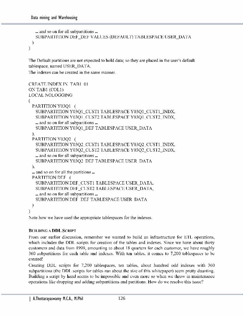
Data mining and Warehousing
| A.Thottarayaswamy M.C.A., M.Phil 126
… …
’
… …
… …
… …
… …

Data mining and Warehousing
| A.Thottarayaswamy M.C.A., M.Phil 127
–
… …
’
–
‘ ’ ’ ’ ’
’
–
’
–

Data mining and Warehousing
| A.Thottarayaswamy M.C.A., M.Phil 128
‘ ’ ’ ’
‘ ’
…
…
’
‘ ’
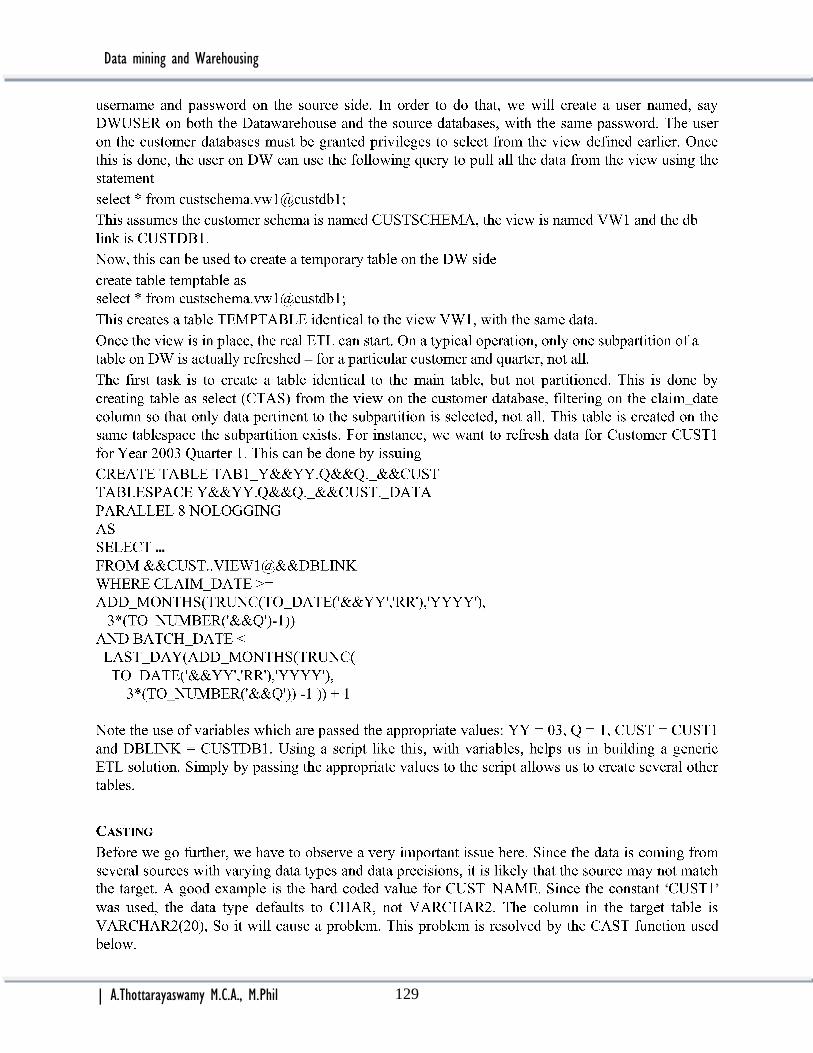
Data mining and Warehousing
| A.Thottarayaswamy M.C.A., M.Phil 129
–
…
‘ ’

Data mining and Warehousing
| A.Thottarayaswamy M.C.A., M.Phil 130
‘ ’

Data mining and Warehousing
| A.Thottarayaswamy M.C.A., M.Phil 131
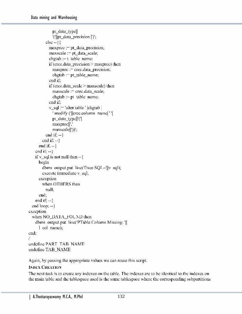
Data mining and Warehousing
| A.Thottarayaswamy M.C.A., M.Phil 132

Data mining and Warehousing
| A.Thottarayaswamy M.C.A., M.Phil 133
‘

Data mining and Warehousing
| A.Thottarayaswamy M.C.A., M.Phil 134
…
–
–

Data mining and Warehousing
| A.Thottarayaswamy M.C.A., M.Phil 135
’
‘ ’
‘ ’
…
…
…
–
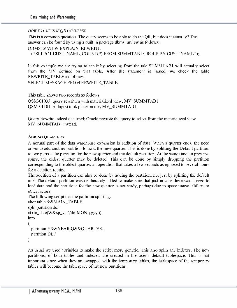
Data mining and Warehousing
| A.Thottarayaswamy M.C.A., M.Phil 136
‘ ’
–
‟
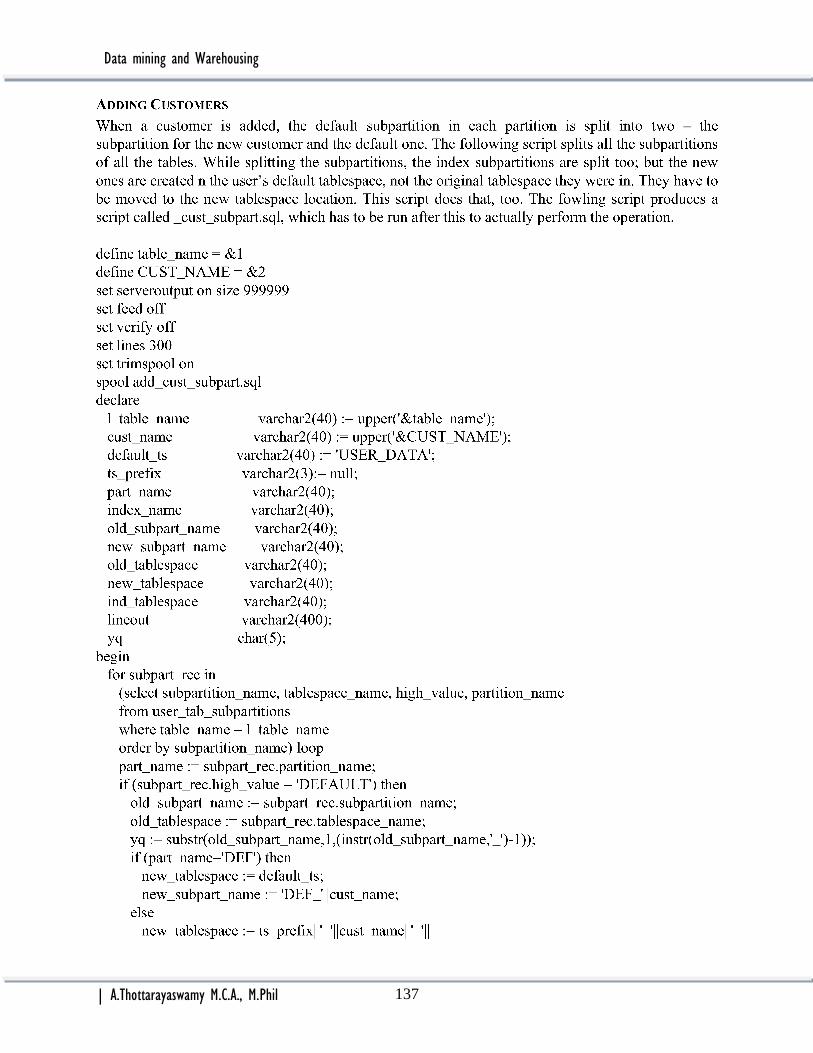
Data mining and Warehousing
| A.Thottarayaswamy M.C.A., M.Phil 137
–
‟
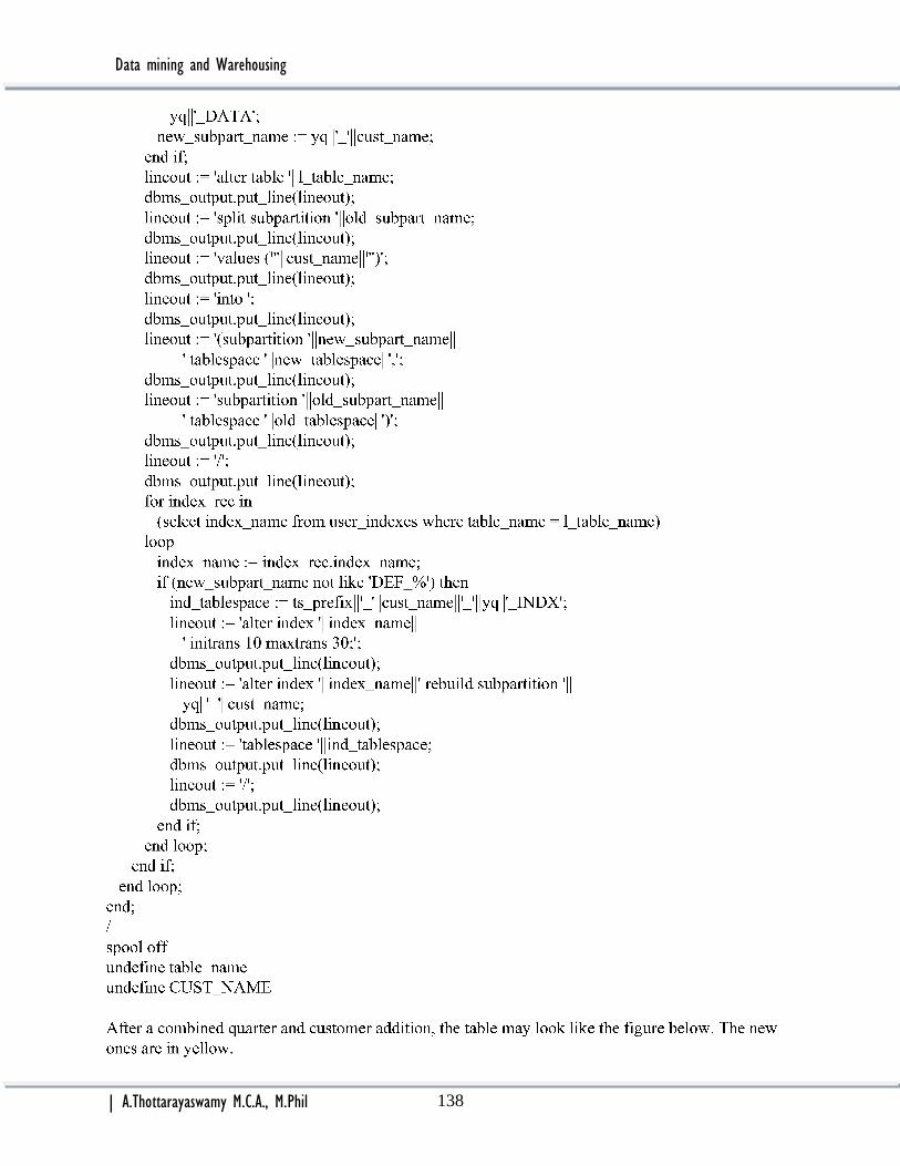
Data mining and Warehousing
| A.Thottarayaswamy M.C.A., M.Phil 138

Data mining and Warehousing
| A.Thottarayaswamy M.C.A., M.Phil 139
’
–
–
Data mining and Warehousing
| A.Thottarayaswamy M.C.A., M.Phil 140
‘ ’
…

Data mining and Warehousing
| A.Thottarayaswamy M.C.A., M.Phil 141
–
‘ ’
–
–
–
–
–
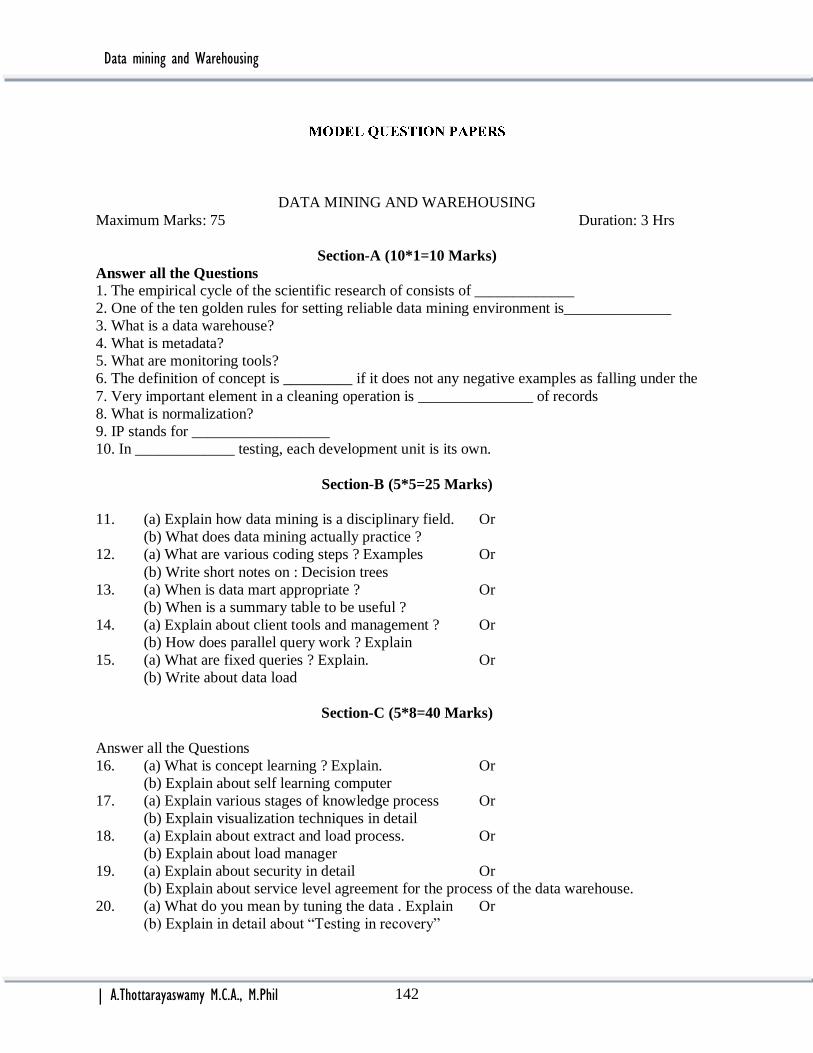
Data mining and Warehousing
| A.Thottarayaswamy M.C.A., M.Phil 142
DATA MINING AND WAREHOUSING
Maximum Marks: 75 Duration: 3 Hrs
Section-A (10*1=10 Marks)
Answer all the Questions
1. The empirical cycle of the scientific research of consists of _____________
2. One of the ten golden rules for setting reliable data mining environment is______________
3. What is a data warehouse?
4. What is metadata?
5. What are monitoring tools?
6. The definition of concept is _________ if it does not any negative examples as falling under the
7. Very important element in a cleaning operation is _______________ of records
8. What is normalization?
9. IP stands for __________________
10. In _____________ testing, each development unit is its own.
Section-B (5*5=25 Marks)
11. (a) Explain how data mining is a disciplinary field. Or
(b) What does data mining actually practice ?
12. (a) What are various coding steps ? Examples Or
(b) Write short notes on : Decision trees
13. (a) When is data mart appropriate ? Or
(b) When is a summary table to be useful ?
14. (a) Explain about client tools and management ? Or
(b) How does parallel query work ? Explain
15. (a) What are fixed queries ? Explain. Or
(b) Write about data load
Section-C (5*8=40 Marks)
Answer all the Questions
16. (a) What is concept learning ? Explain. Or
(b) Explain about self learning computer
17. (a) Explain various stages of knowledge process Or
(b) Explain visualization techniques in detail
18. (a) Explain about extract and load process. Or
(b) Explain about load manager
19. (a) Explain about security in detail Or
(b) Explain about service level agreement for the process of the data warehouse.
20. (a) What do you mean by tuning the data . Explain Or
(b) Explain in detail about “Testing in recovery”

Data mining and Warehousing
| A.Thottarayaswamy M.C.A., M.Phil 143