data mining - carl h. lindner college of business objectives • motivate you to approach data...
TRANSCRIPT

Data Mining Day One
November, 5-6 2015
Instructor:
Kristofer Still

Schedule
8:00 AM 9:00 AM Networking
9:00 AM 10:30 AM Session 1
10:30 AM 10:45 AM Break
10:45 AM 12:15 PM Session 2
12:15 PM 1:00 PM Lunch
1:00 PM 2:30 PM Session 3
2:30 PM 3:00 PM Break
3:00 PM 4:30 PM Session 4
Agenda
Day One
• Overview
• The Data Mining Process
• Hands on examples
Day Two
• Case Study
• Data Mining for Unstructured Data
• Demos of other Helpful Data Mining Tools and Resources

Learning objectives
• Motivate you to approach data mining like any other managed project or process.
• Gain a set of tools that provide a systematic process by which you can understand the nature of your data and how to get the most out of it
• Understand how to evaluate models and some ways to potentially improve a model’s performance

Why R?
• Not the answer for everyone
• Pros and cons
• Recent developments and trends
• Future

Data
• Data is always involved
• Usually more data than people can keep track of
• Terabytes of data – now petabytes
– Example “A Million Model in Minutes”
• Data is more complex
Questions About Your Data
• How much data do I have and at what rate do I expect it
to grow?
• How is it stored?
• Is it secure and recoverable?
• What’s important?
• How can I convert data into insights?

Finding Insights
• What is the chance that an event will occur and what will be the magnitude of that event?
• What patterns are there in my database and which are significant?
• How can I group and classify the entities in my data?
• What relationships exist in my data?
• Can I detect anomalies in my data?
• What do I expect to happen to measures over time?

Sample Data
• Example Database of Customers
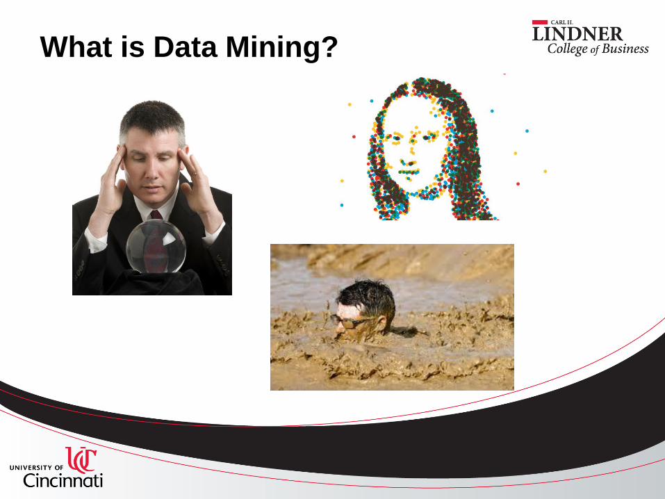
What is Data Mining?

What is Data Mining?

What is Data Mining?
• “the nontrivial process of identifying valid, novel, potentially useful, and ultimately understandable patterns in data.” --- Fayyad
• “finding interesting structure (patterns, statistical models, relationships) in data bases”.--- Fayyad, Chaduri and Bradley
• “a knowledge discovery process of extracting previously unknown, actionable information from very large data bases”--- Zornes
• “ a process that uses a variety of data analysis tools to discover patterns and relationships in data that may be used to make valid predictions.” ---Edelstein

What is Data Mining?
da·ta min·ing
noun
Computing
noun: data mining; noun: datamining
1.
the practice of examining data using various modeling techniques in order to generate new information or insight, detect patterns and relationships, and ultimately make valid predictions. -Shaffer (2014)
2.
The process by which an organization seeks to utilize its data assets to generate value for its stakeholders.-Still (2014) (see also 1.)

Statistics vs. Data Mining
• Statistics is part of data mining – ex. Determining the
signal from the noise, significance of findings (inference),
estimating probabilities. In statistics data is often
collected to answer a specific question.
• Data Mining – much broader, entire process of data
analysis, including data cleaning, preparation and
visualization. Data has typically been collected in some
manner.

Statistics vs. Data Mining
Statistics
• Particular model with
specific parameters and
assumptions about the
model errors
• In addition to accuracy,
often equally concerned
with interpretation and
range of results
• Generally not
computationally intensive
Data Mining
• Models are flexible and
often better suited for
non-linear relationships in
data
• Prediction accuracy is
most important
• Computationally intensive

Data Mining Process Models
• Six Sigma (Design, Measure, Analyze, Improve, Control)
• KDD (Knowledge Discovery in Databases)
• SEMMA (Sample, Explore, Modify, Model, Assess)
• CRISP-DM (Cross Industry Standard Process for Data Mining

Six Sigma Model - DMAIC

KDD Model

SEMMA Model

CRISP-DM

What do these have in common?
• Business understanding
• Understanding the data through exploration
• Data preparation
• Modeling
• Interpretation/Evaluation
• Recommendation/Implementation

Why?
Like most relationships things go well when needs are met.
“We have to protect our phoney, baloney jobs here, gentlemen!”
-Governor William J. Le Petomane, Blazing Saddles (1974)

Business Understanding Overview
• Assess situation
• Set goals
• Create Plan

Business Understanding – Assess
• Current state/desired state
• Customer
• Players (governors, partners, gatekeepers, advocates)
• Cost/benefit
• Resources (hardware/software, data, expertise, time, budget)
• Security/access
• Deployment

Business Understanding – Set
Goals
• Business and data mining goal?
• SMART
• Qualify
• Risk

Business Understanding – Set
Goals
• Measuring business success?
Business Understanding – Set
Goals
• Measuring data mining success?

Business Understanding – Set
Goals
Business goals:
• Reduce customer churn by 5% in 6 months among customers with a profit margin of 10% or more.
• Reduce wire fraud in the commercial bank by 10 percent within three months of deploying new anomaly detection algorithm, 15 percent within six months, and 25 percent within one year.

Understanding your data
• Does your data have what it takes?
– Suitable?
– Sufficient?
– High information content?
– Challenges

Source
• Quantity
• Veracity (surveys, social media/web, 3rd party source, deception, temporal, missing)
• Measurement/Collection
• How are systems, databases, entities related
– IDs
– Attributes and dimensions
– Aggregation

Veracity
Characterizing your data
• Granularity
• Consistency
• Contamination
• Interactions

Granularity
• Too little?
• Too much?
• Date/time considerations
• Geographic considerations

Consistency
• Redundancy (duplication and naming)
• Value labels (single system)
• Change in definition or measurement
• Latency
• Operational changes or changes in external environment
• Truncation

Pollution
• Leaks from the future
• Duplicate records
• Invalid values
• Errors

Outliers
• Global v. Local
• Causes include
– Poor data quality / contamination
– Low quality measurements, malfunctioning equipment, manual error
– Correct but exceptional data

Missing data
• No data for a field or entire record
• Why missing?

Domain
• All permissible values for a variable
• Conditional
– Influenced by other variable
– Influenced by business rules
Default values
• Usually related to missing or empty values, but could be conditional
– E.g. 9999, 0, -1, >N
• What are the potential concerns if you treated them as valid values?

Sparsity
• Inputs usually related to categorical inputs
• Target e.g. bankruptcy, medical studies, insurance, fraud detection, payment, security

How to manage sparsity
• Inputs – transform the input
• Transform the data
– Sampling
– Introduce bias
Data Exploration
• Dimension
• Data types
• Summary measures
– Centrality - mean, median, mode
– Dispersion – range, variation, standard deviation
– Skewness and kurtosis
– Relationship – correlation
• Plots – box plots, histograms, pie charts, scatterplots, parallel coordinates, heat maps

Data Types
Qualitative
• Categorical – data as named classes or levels of an attribute
– Nominal - differentiates between items and subjects base on their names e.g. gender, race, style, form
– Ordinal – allows for a rank order but nothing can be said about degree of difference between them. e.g. true/false (binary), rankings, income or class

Data Types
Quantitative
• Numeric (continuous) – has numeric value and a natural order
– Interval – has interpretable differences but no true zero and can’t be multiplied or divided e.g. Dates, temperature (Yes, Kelvin would be an exception, but resist the urge to raise your hand and out yourself as a BIG nerd.)
– Ratio – specifies “how much” (magnitude) or “how many“ (count) of something. Unlike interval has a non-arbitrary zero point so came make comparisons like “twice as” e.g. age, length, mass, elapsed time
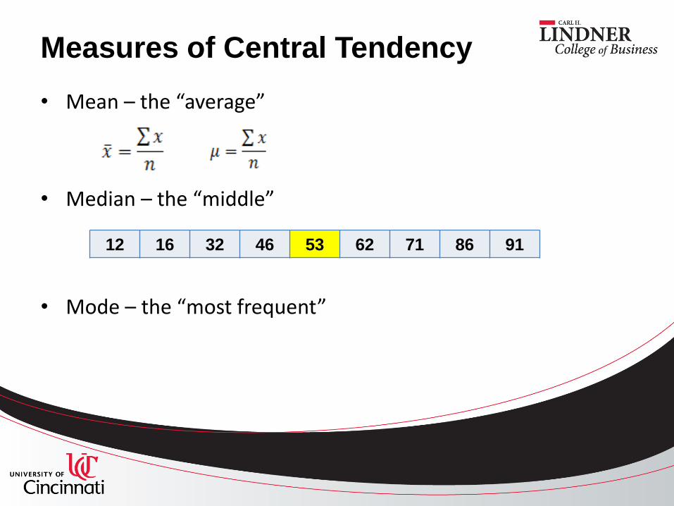
Measures of Central Tendency
• Mean – the “average”
• Median – the “middle”
• Mode – the “most frequent”
12 16 32 46 53 62 71 86 91

Measures of Central Tendency

Measures of Central Tendency
Remove Outlier:
mean - 6.3
median - 4.5
range - 17

Measures of Dispersion
• Range – Max minus Min • Variance –the average squared difference of the scores from the
mean:
𝑠2 =(𝑥 − 𝑥 )2
𝑛 − 1
• Standard deviation – the square root of the variance:
𝑠 =(𝑥 − 𝑥 )2
𝑛 − 1
• Variance vs. standard deviation?
Two Types of Variation

Variation
• Common Cause
• Special Cause

Measures of Variability

Skewness and Kurtosis
• Skewness - measures how symmetric a distribution is:
𝑠𝑘𝑒𝑤𝑛𝑒𝑠𝑠 =(𝑥 − 𝑥 )3
(𝑛 − 1)𝑠3
• Standard deviation – indicates how peaked or flat a distribution is compared to a normal distribution:
𝑘𝑢𝑟𝑡𝑜𝑠𝑖𝑠 =(𝑥 − 𝑥 )4
(𝑛 − 1)𝑠4

Skewness and kurtosis

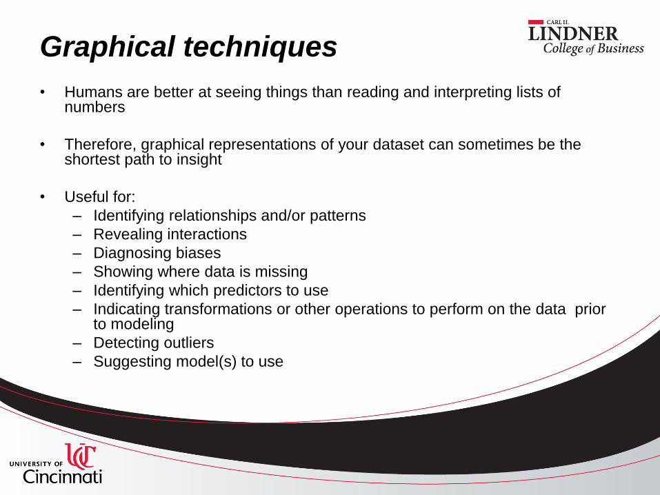
Graphical techniques
• Humans are better at seeing things than reading and interpreting lists of numbers
• Therefore, graphical representations of your dataset can sometimes be the shortest path to insight
• Useful for:
– Identifying relationships and/or patterns
– Revealing interactions
– Diagnosing biases
– Showing where data is missing
– Identifying which predictors to use
– Indicating transformations or other operations to perform on the data prior to modeling
– Detecting outliers
– Suggesting model(s) to use

Histogram
• A histogram divides the levels of a variable into equal-sized bins and then counts then number of points in the dataset that belong in each bin.

Histogram
• Great tool to summarize data. Can see center, spread,
as well as issues with skew, outliers, or bimodality.

Box and Whiskers or Box Plot (Tukey)

Box and Whiskers or Box Plot (Tukey)

Box and Whiskers or Box Plot (Tukey)
The Box:
– Median – the line on drawn on the box
– Lower quartile – number 25% of the data lies below;
median between minimum and the overall median
– Upper quartile – number 75% of the data lies below;
median between maximum and the overall median

Box and Whiskers or Box Plot (Tukey)
The whiskers variation 1:
– Draw line from the top of the box (Q3) to the max and
the bottom of the box (Q1) to the minimum

Box and Whiskers or Box Plot (Tukey)
The whiskers variation 2:
– Calculate the interquartile range: IQR = Q3 – Q1
– Then calculate:
• L1 = Q1 – 1.5 * IQR
• L2 = Q1 – 3.0 * IQR
• U1 = Q3 + 1.5 * IQR
• U2 = Q1 + 3.0 * IQR
– Whiskers drawn from Q1 to smallest point > L1 and from Q3 to
largest point smaller than U1
– Points between L1 and L2 and U1 and U2 are drawn as a small
circle
– Points beyond L2 and U2 are drawn as large circles
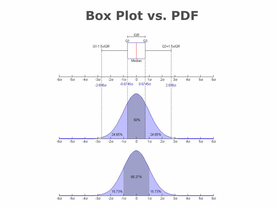
Box Plot vs. PDF


Scatterplot
• Allows you to see potential associations between two or
more variables
• You can also see the direction and shape of that
relationship
• Finally, you can identify if that relationship changes as
one of the variables changes (homo/heteroscedastic)

Scatterplot (examples)
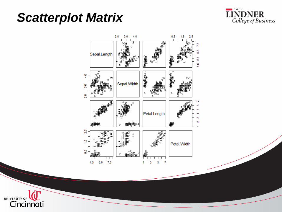
Scatterplot Matrix

Linear Regression

Data preparation
• Measure quality
• Test assumptions
• Validate! Validate! Validate!

Modeling
• Choose modeling technique(s)
• Fit model(s)
• Evaluate model(s)
• Tune model(s)
Wash, rinse, repeat until you have the “best” model or
collection of models

Choose wisely….
• Suitability
– Type of prediction
– Types of observations
– Shape
– Interaction
• Assumptions
• Missing data
• Scalability
• Interpretability
• Audience

Linear Regression
𝑦 = 𝑚𝑥 + 𝑏
𝑚 = 𝑥𝑦 − 𝑥 𝑦
𝑥 2 − (𝑥 )2
𝑏 = 𝑦 − 𝑚𝑥

Pattern of Data Not Linear
• More predictors than just one can be used.
– Multiple Regression
• Transformations can be applied to the predictors.
• Predictors can be multiplied together and used as terms
in the equation.
• Modifications can be made to accommodate response
predictions that just have yes/no or 0/1 values.

Logistic Regression
• Pay/No Pay, Bankruptcy, Re-Admittance
• Estimation no longer least squares
• Now likelihood approach
• MLE (maximum likelihood estimation) of logit regression
• Mean Residual Deviance – compare model with model complexity (compare to adjusted R2)
• Residual Deviance – won’t account for model complexity (compare to R2)
• Smaller Mean Residual Deviance is better

Cluster Analysis • Algorithm that will take a dataset and attempt to divide its
entities into n groups based on their attribute values.
• Determines an optimal (may not be unique solution) set
of groups that maximizes both the with in group similarity
and distance between groups
• High school, The sorting hat, laundry
• e.g. customer types, fraud detection, location selection

Clustering
• “Sorting the laundry”
– White clothes vs. color clothes (easy)
– White short with color stripes?
– Gray Shirt?
• Clustering in business applications much more difficult
– Very dynamic
– Ever changing
• How many clusters?
– This is key

Clustering

Clustering
• Also used to detect outliers.
– Which records stand out from the clusters
Example:
A sale on men’s suits is being held in all branches of a
department store for southern California. All stores with
these characteristics have seen at least a 100% jump in
revenue since the start of the sale except one. It turns out
that this store had, unlike the others, advertised via radio
rather than television.
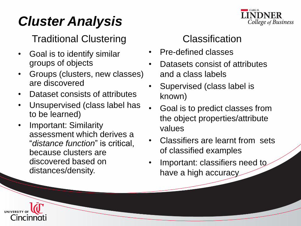
Cluster Analysis
Traditional Clustering
• Goal is to identify similar groups of objects
• Groups (clusters, new classes) are discovered
• Dataset consists of attributes
• Unsupervised (class label has to be learned)
• Important: Similarity assessment which derives a “distance function” is critical, because clusters are discovered based on distances/density.
Classification
• Pre-defined classes
• Datasets consist of attributes
and a class labels
• Supervised (class label is
known)
• Goal is to predict classes from
the object properties/attribute
values
• Classifiers are learnt from sets
of classified examples
• Important: classifiers need to
have a high accuracy

Clustering
• Happy medium between homogeneous groups and the
fewest number of clusters.
• How useful is a cluster of one?
• Or a cluster for each individual point?

Two types of Clustering
• Hierarchical
– Tree
• Smallest clusters merge together
• Agglomerative vs. Divisive
– Clusters defined by the data
• Non-Hierarchical
– Single pass method
– Reallocation method
• User defines 10 clusters, but data is clearly 13

Nearest Neighbor
• Your next door neighbor’s income is $100,000
– How much do you make?
• Your next door neighbor’s income is $30,000
– How much do you make?
• Assumptions are being made
• Consider other variables (broader definition of neighbor):
– School attended and degree
– Job title
– Length of job

Nearest Neighbor
• Apple
– Closer to Orange or Banana?
• Toyota Corolla
– Closer to a Honda Civic or a Porsche?
• Simply Stated
– Objects that are “near” to each other will have similar
prediction values as well. Therefore if you know the
prediction value of one of the objects you can predict
it for it’s nearest neighbors.
Nearest Neighbor
• Applications
– Text Retrieval
– Search Algorithms
– Stock Market Data
– “Customers who bought this also bought”
– Movie preferences

K Nearest Neighbor (KNN)
• Let’s vote on it
– Many is better than one
• All of your neighbor’s have income > $100,000
– How much do you make?
– Are you a little more confident in your guess?
• A vote of ¾ of your neighbors compared to a single
neighbor would be more accurate.
• How confident are we?
• Can we measure this?

K Nearest Neighbor (KNN)
• The distance to the nearest neighbor provides a level of confidence.
• If the neighbor is very close or an exact match then there is much higher confidence in the prediction than if the nearest record is a great distance from the unclassified record.
• The degree of homogeneity amongst the predictions within the K nearest neighbors can also be used. If all the nearest neighbors make the same prediction then there is much higher confidence in the prediction than if half the records made one prediction and the other half made another prediction.

N-Dimensional Space
• In order to determine near vs. far we need to define a
space where distance can be calculated
– Neighborhoods for Income
• If we have 5 predictors then we have a 5 dimensional
space
• Imagine 1,000 or 50,000 predictors
• Clustering – typically 1 predictor to each dimension
• Nearest Neighbor – dimensions are stretched
– Basically weighting one more than another when
calculating the distance

Clustering vs. Nearest Neighbor

Decision Trees
• Predictive Model viewed as a tree
• Each branch of the tree is a classification method
• Divides up data at each branch without losing data
• Very easy to understand and interpret
– Opposite of the Neural Network (black box)
• Good at handling raw data and minimizes pre-
processing
• Excel at complex real world problems, computationally
cheap
• Used for Exploration, Data Processing, Prediction

Decision Trees

Decision Trees
• Over fitting is when your tree (or any data mining
algorithm for that matter) pays attention to parts of the
data that are irrelevant (i.e. fits noise)
• Over fitting can cause your model to make less accurate
predictions on new data. (i.e. less robust)
• Can use statistical tests to detect over fitting. In this case
a chi-square test. Would this result have happened by
chance?

Decision Trees
• Start at the bottom of your tree and do a chi-square test
on the terminal nodes to determine:
If there was no relationship between the input and target,
what’s the chance I would have the same result?
• Remove (prune) those nodes
• Finding the simplest (parsimonious) tree for your data
Random Forest
• Grow many trees varying the sample and variables used
to grow the tree randomly
• Prediction chosen is the mode of the predictions of all
the individual trees in the “forest”
Neural Networks
• Approximate representation of how are brains are
organized and how we “learn.”
• They “learn” and adapt, but so do other models

Neural Networks
• Our brain is made up of dozens of billions of neurons
Neural Networks
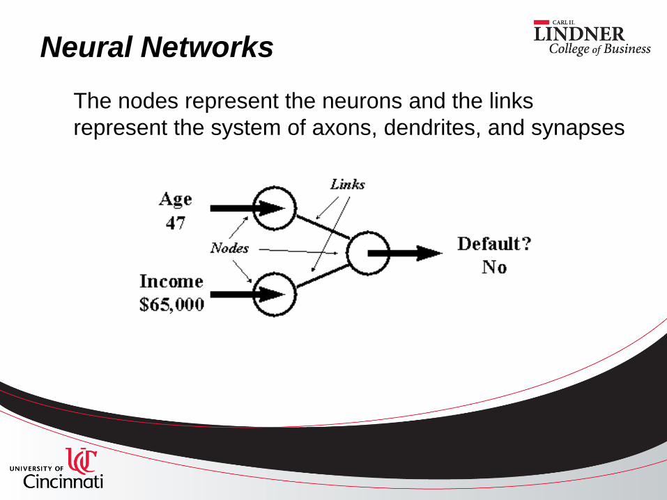
The nodes represent the neurons and the links
represent the system of axons, dendrites, and synapses
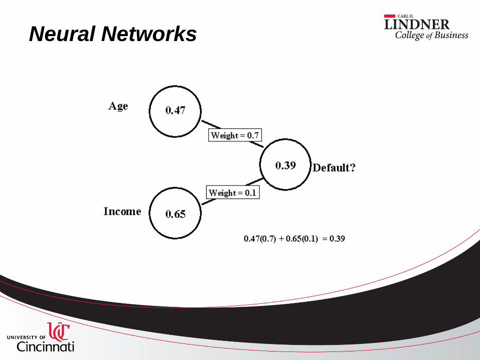
Neural Networks

Neural Networks

Neural Networks
• Requires lots of pre-processing of the data
– Standardizing variables can be very important
• Very powerful predictive modeling techniques
– But at a cost
• Ease of use
• Ease of deployment
• Over fitting – they are exceptional at training noise

Evaluating Models
• Measure quality
• Test assumptions
• Validate! Validate! Validate!

Accuracy Precision vs.

Accuracy Precision vs.

Is this Process Accurate?
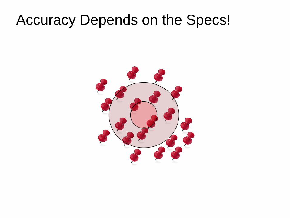
Accuracy Depends on the Specs!

Accuracy Depends on the Specs!
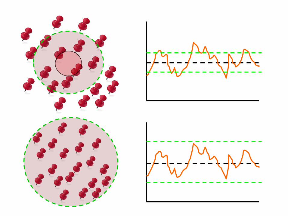

Question the Specs
“If the facts don’t fit the theory, change the facts. - Albert Einstein

Control Charts
This Process is IN CONTROL

Is this process Accurate?
HINT – What are the Specs?
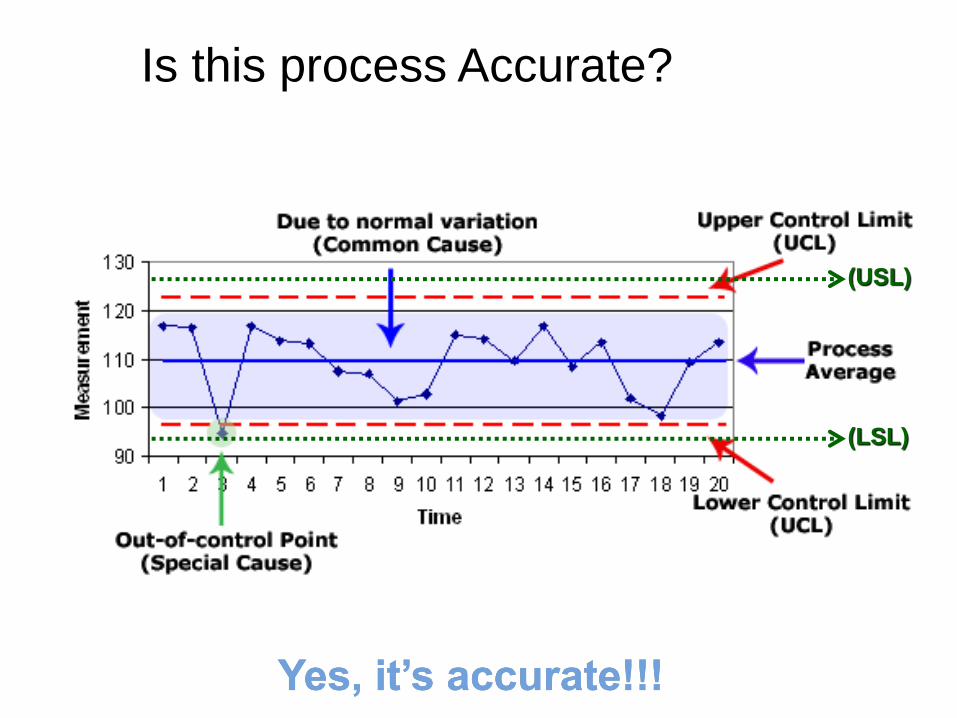
Is this process Accurate?
Yes, it’s accurate!!!
(USL)
(LSL)

Is this process Accurate?
NO, it’s NOT accurate!!!
(USL)
(LSL)

Measuring Success
• Regression
– “Regression toward the mean”
– Error is normal
– “Independent” is an important assumption
– “OLS” (ordinary least squared)
• Why is it ordinary? Because it’s linear (not weighted)
• Minimize the sum of the squared residuals
– Unconstant variation is called…

Measuring Success
Unconstant variation is called…


Measuring Success
Bigger is better (unless it’s too good!)
R2 – measures goodness of fit
Adjusted R2 – adjusts for number of explanatory terms. The more variables the more error is introduced into the model.
Small p-value – reject the null hypothesis
f-test and t-test equivalent

Measuring Success
• MSE – Mean Squared Error (lower the better)
– Risk Function
– Quantify difference between implied values of estimator and true values
– “Squared Error Loss” (quadratic loss) – average of the squares of the error
– RMSE is the square root of MSE (same unit as y-axis)
• Greatest reduction in MSE or RMSE often determines the winners of analytics competitions on sites like Kaggle
– e.g. reduction in RMSE of Netflix’s recommendation engine
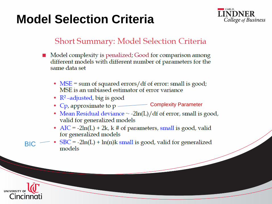
Model Selection Criteria
Complexity Parameter
BIC

Variable Selection
• Forward – one at a time – Use f-test to rank – One by one procedure (look at p-value)
• Backwards – remove one at a time – Examine model performance after each decision – Once removed, never comes back – Need rule to stop
• Stepwise – combination of forward and backward – Might have one variable in, then out, then back in
• “All possible” “Best subset” “Exhaustive search” – Fit model with all possible combination of variables and
compare performance measures

Variable Selection
• First three methods are one dimensional
• Can only use complete cases (i.e. must have value for each variable)
• Low ratio of cases to variables and excessive collinearity can disrupt selection
• Can disrupt logical groupings
• Don’t ignore your own judgment and intuition about your data
• Can’t make something out of nothing (GIGO)

Deployment
• End product
• Load
• Maintenance and management
• Monitor and measure business outcomes
• Best practices
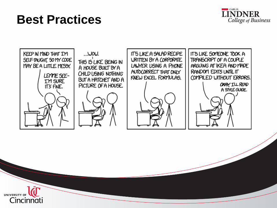
Best Practices