Data Mining Meets HCI:Making Sense of Large Graphs

Duen Horng (Polo) Chau

July 2012CMU-ML-12-103

Data Mining Meets HCI:Making Sense of Large Graphs

Duen Horng (Polo) Chau

July 2012CMU-ML-12-103

Machine Learning DepartmentCarnegie Mellon University

Pittsburgh, PA 15213

Thesis Committee:Christos Faloutsos, ChairJason I. Hong, Co-ChairAniket Kittur, Co-Chair

Jiawei Han, UIUC

Submitted in partial fulfillment of the requirementsfor the degree of Doctor of Philosophy.

Copyright c© 2012 Duen Horng (Polo) Chau

This research is supported by: National Science Foundation grants IIS-0705359, IIS-0968484,IIS-0970179, IIS-1017415, OCI-0943148, NSC 99-2218-E-011-019, NSC 98-2221-E-011-105;Symantec Research Labs Graduate Fellowship (2009, 2010); IBM Faculty Award, Google FocusedResearch Award; Army Research Laboratory W911NF-09-2-0053.

The views and conclusions contained in this document are those of the author and should notbe interpreted as representing the official policies, either expressed or implied, of any sponsoringinstitution, the U.S. government or any other entities.

Keywords: Graph Mining, Data Mining, Machine Learning, Human-ComputerInteraction, HCI, Graphical Models, Inference, Big Data, Sensemaking, Visu-alization, eBay Auction Fraud Detection, Symantec Malware Detection, BeliefPropagation, Random Walk, Guilt by Association, Polonium, NetProbe, Apolo,Feldspar, Graphite

For my parents and brother.

iv

AbstractWe have entered the age of big data. Massive datasets are now

common in science, government and enterprises. Yet, making senseof these data remains a fundamental challenge. Where do we start ouranalysis? Where to go next? How to visualize our findings?

We answers these questions by bridging Data Mining and Human-Computer Interaction (HCI) to create tools for making sense of graphswith billions of nodes and edges, focusing on:

(1) Attention Routing: we introduce this idea, based on anomalydetection, that automatically draws people’s attention to interestingareas of the graph to start their analyses. We present three exam-ples: Polonium unearths malware from 37 billion machine-file rela-tionships; NetProbe fingers bad guys who commit auction fraud.

(2) Mixed-Initiative Sensemaking: we present two examplesthat combine machine inference and visualization to help users lo-cate next areas of interest: Apolo guides users to explore large graphsby learning from few examples of user interest; Graphite finds inter-esting subgraphs, based on only fuzzy descriptions drawn graphically.

(3) Scaling Up: we show how to enable interactive analytics oflarge graphs by leveraging Hadoop, staging of operations, and ap-proximate computation.

This thesis contributes to data mining, HCI, and importantly theirintersection, including: interactive systems and algorithms that scale;theories that unify graph mining approaches; and paradigms that over-come fundamental challenges in visual analytics.

Our work is making impact to academia and society: Poloniumprotects 120 million people worldwide from malware; NetProbe madeheadlines on CNN, WSJ and USA Today; Pegasus won an open-source software award; Apolo helps DARPA detect insider threatsand prevent exfiltration.

We hope our Big Data Mantra “Machine for Attention Routing,Human for Interaction” will inspire more innovations at the crossroadof data mining and HCI.

vi

AcknowledgmentsTo everyone in my Ph.D. journey, and in life—this is for you.Christos, only with your advice, support and friendship can I pursue this ambi-

tious thesis. Your generosity and cheerful personality has changed my world. Jasonand Niki, thanks for your advice and ideas (esp. HCI-related). Having 3 advisors isan amazing experience! Jiawei, thank you for your terrific insights and advice.

Jeff Wong, thanks for your brotherly support, research idea, and insider jokes.Isabella, Bill, Robin and Horace: you make me feel at home when I escape fromwork. Queenie Kravitz, thanks for our precious friendship; your are the best HCIIprogram coordinator I’ve ever known. Carey Nachenberg, thank you for supportingmy research (esp. Polonium), and our friendship with ShiPu; it’s a treasure.

I thank Brad Myers, Jake Wobbrock, Andy Ko, Jeff Nichols, and AndrewFaulring for nurturing my enthusiasm in research; you confirmed my passion. Men-tors and friends at Symantec and Google, thank you for your guidance and friend-ship that go well beyond my internships: Darren Shou, Arun Swami, Jeff Wilhelmand Adam Wright.

Christina Cowan, you and Christos are the two most cheerful people in thewhole world! Your every presence brightens my days. Michalis Faloutsos, thanksfor seeing the entrepreneur in me.

My academic siblings in the DB group, I treasure our joyous moments (esp.trips) and collaboration: Leman Akoglu, U Kang, Aditya Prakash, Hanghang Tong,Danai Koutra, Vagelis Papalexakis, Rishi Chandy, Alex Beutel, Jimeng Sun, SpirosPapadimitriou, Tim Pan, Lei Li, Fan Guo, Mary McGlohon, Jure Leskovec, andBabis Tsourakakis.

I am blessed to work with Marilyn Walgora, Diane Stidle, Charlotte Yano,Indra Szegedy, David Casillas, and Todd Seth, who are meticulous with every ad-ministrative detail.

I thank Daniel Neill, Bilge Mutlu, Jake Wobbrock, and Andy Ko for being mychampions during job search, Justine Cassell and Robert Kraut for their advice.

I’m grateful to have celebrated this chapter of my life with many dear friends:Robert Fisher, Katherine Schott, Mladen Kolar and Gorana Smailagic, Alona Fysheand Mark Holzer, Brian Ziebart and Emily Stiehl, Edith Law, Matt Lee, TawannaDillahunt, Prashant and Heather Reddy, James Sharpnack and Vicky Werderitch (Iwon’t forget the night I got my job!), Felipe Trevizan, Sue Ann Hong, Dan Morris,Andy Carlson, Austin McDonald, and Yi Zhang. I thank my sports buddies, whokeep me sane from work: Lucia Castellanos, Michal Valko, Byron Boots, NeilBlumen, and Sangwoo Park.

I thank my friends, collaborators, and colleagues for their advice, friendship,and help with research: Jilles Vreeken, Tina Eliass-Rad, Partha Talukdar, ShashankPandit, Sam Wang, Scott Hudson, Anind Dey, Steven Dow, Scott Davidoff, Ian Li,Burr Settles, Saket Navlakha, Hai-son Lee, Khalid El-Arini, Min Xu, Min KyungLee, Jeff Rzeszotarski, Patrick Gage Kelly, Rasmus Pagh, and Frank Lin.

Mom, dad, brother: I love you and miss you, though I never say it.

viii

Contents

1 Introduction 11.1 Why Combining Data Mining & HCI? . . . . . . . . . . . . . . . 21.2 Thesis Overview & Main Ideas . . . . . . . . . . . . . . . . . . . 4

1.2.1 Attention Routing (Part I) . . . . . . . . . . . . . . . . . 41.2.2 Mixed-Initiative Graph Sensemaking (Part II) . . . . . . . 51.2.3 Scaling Up for Big Data (Part III) . . . . . . . . . . . . . 7

1.3 Thesis Statement . . . . . . . . . . . . . . . . . . . . . . . . . . 91.4 Big Data Mantra . . . . . . . . . . . . . . . . . . . . . . . . . . 91.5 Research Contributions . . . . . . . . . . . . . . . . . . . . . . . 101.6 Impact . . . . . . . . . . . . . . . . . . . . . . . . . . . . . . . . 11

2 Literature Survey 132.1 Graph Mining Algorithms and Tools . . . . . . . . . . . . . . . . 132.2 Graph Visualization and Exploration . . . . . . . . . . . . . . . . 162.3 Sensemaking . . . . . . . . . . . . . . . . . . . . . . . . . . . . 17

I Attention Routing 19

3 NetProbe: Fraud Detection in Online Auction 213.1 Introduction . . . . . . . . . . . . . . . . . . . . . . . . . . . . . 223.2 Related Work . . . . . . . . . . . . . . . . . . . . . . . . . . . . 24

3.2.1 Grass-Roots Efforts . . . . . . . . . . . . . . . . . . . . . 243.2.2 Auction Fraud and Reputation Systems . . . . . . . . . . 24

3.3 NetProbe: Proposed Algorithms . . . . . . . . . . . . . . . . . . 253.3.1 The Markov Random Field Model . . . . . . . . . . . . . 253.3.2 The Belief Propagation Algorithm . . . . . . . . . . . . . 263.3.3 NetProbe for Online Auctions . . . . . . . . . . . . . . . 28

ix

3.3.4 NetProbe: A Running Example . . . . . . . . . . . . . . 293.3.5 Incremental NetProbe . . . . . . . . . . . . . . . . . . . 30

3.4 Evaluation . . . . . . . . . . . . . . . . . . . . . . . . . . . . . . 323.4.1 Performance on Synthetic Datasets . . . . . . . . . . . . 333.4.2 Accuracy of NetProbe . . . . . . . . . . . . . . . . . . . 343.4.3 Scalability of NetProbe . . . . . . . . . . . . . . . . . . . 343.4.4 Performance on the EBay Dataset . . . . . . . . . . . . . 353.4.5 Data Collection . . . . . . . . . . . . . . . . . . . . . . . 353.4.6 Efficiency . . . . . . . . . . . . . . . . . . . . . . . . . . 353.4.7 Effectiveness . . . . . . . . . . . . . . . . . . . . . . . . 353.4.8 Performance of Incremental NetProbe . . . . . . . . . . . 36

3.5 The NetProbe System Design . . . . . . . . . . . . . . . . . . . . 373.5.1 Current (Third Party) Implementation . . . . . . . . . . . 373.5.2 Crawler Implementation . . . . . . . . . . . . . . . . . . 383.5.3 Data Structures for NetProbe . . . . . . . . . . . . . . . . 393.5.4 User Interface . . . . . . . . . . . . . . . . . . . . . . . . 41

3.6 Conclusions . . . . . . . . . . . . . . . . . . . . . . . . . . . . . 423.6.1 Data Modeling and Algorithms . . . . . . . . . . . . . . 433.6.2 Evaluation . . . . . . . . . . . . . . . . . . . . . . . . . 433.6.3 System Design . . . . . . . . . . . . . . . . . . . . . . . 43

4 Polonium: Web-Scale Malware Detection 454.1 Introduction . . . . . . . . . . . . . . . . . . . . . . . . . . . . . 454.2 Previous Work & Our Differences . . . . . . . . . . . . . . . . . 48

4.2.1 Research in Malware Detection . . . . . . . . . . . . . . 494.2.2 Research in Graph Mining . . . . . . . . . . . . . . . . . 50

4.3 Data Description . . . . . . . . . . . . . . . . . . . . . . . . . . 504.4 Proposed Method: the Polonium Algorithm . . . . . . . . . . . . 52

4.4.1 Problem Description . . . . . . . . . . . . . . . . . . . . 534.4.2 Domain Knowledge & Intuition . . . . . . . . . . . . . . 534.4.3 Formal Problem Definition . . . . . . . . . . . . . . . . . 544.4.4 The Polonium Adaptation of Belief Propagation (BP) . . . 554.4.5 Modifying the File-to-Machine Propagation . . . . . . . . 56

4.5 Empirical Evaluation . . . . . . . . . . . . . . . . . . . . . . . . 574.5.1 Single-Iteration Results . . . . . . . . . . . . . . . . . . . 574.5.2 Multi-Iteration Results . . . . . . . . . . . . . . . . . . . 584.5.3 Scalability . . . . . . . . . . . . . . . . . . . . . . . . . 614.5.4 Design and Optimizations . . . . . . . . . . . . . . . . . 61

x

4.6 Significance and Impact . . . . . . . . . . . . . . . . . . . . . . . 624.7 Discussion . . . . . . . . . . . . . . . . . . . . . . . . . . . . . . 634.8 Conclusions . . . . . . . . . . . . . . . . . . . . . . . . . . . . . 65

II Mixed-Initiative Graph Sensemaking 67

5 Apolo: Machine Learning + Visualization for Graph Exploration 695.1 Introduction . . . . . . . . . . . . . . . . . . . . . . . . . . . . . 70

5.1.1 Contributions . . . . . . . . . . . . . . . . . . . . . . . . 715.2 Introducing Apolo . . . . . . . . . . . . . . . . . . . . . . . . . . 72

5.2.1 The user interface . . . . . . . . . . . . . . . . . . . . . . 725.2.2 Apolo in action . . . . . . . . . . . . . . . . . . . . . . . 72

5.3 Core Design Rationale . . . . . . . . . . . . . . . . . . . . . . . 765.3.1 Guided, personalized sensemaking and exploration . . . . 765.3.2 Multi-group Sensemaking of Network Data . . . . . . . . 775.3.3 Evaluating exploration and sensemaking progress . . . . . 775.3.4 Rank-in-place: adding meaning to node placement . . . . 79

5.4 Implementation & Development . . . . . . . . . . . . . . . . . . 795.4.1 Informed design through iterations . . . . . . . . . . . . . 795.4.2 System Implementation . . . . . . . . . . . . . . . . . . 81

5.5 Evaluation . . . . . . . . . . . . . . . . . . . . . . . . . . . . . . 815.5.1 Participants . . . . . . . . . . . . . . . . . . . . . . . . . 815.5.2 Apparatus . . . . . . . . . . . . . . . . . . . . . . . . . . 825.5.3 Experiment Design & Procedure . . . . . . . . . . . . . . 825.5.4 Results . . . . . . . . . . . . . . . . . . . . . . . . . . . 835.5.5 Subjective Results . . . . . . . . . . . . . . . . . . . . . 845.5.6 Limitations . . . . . . . . . . . . . . . . . . . . . . . . . 86

5.6 Discussion . . . . . . . . . . . . . . . . . . . . . . . . . . . . . . 865.7 Conclusions . . . . . . . . . . . . . . . . . . . . . . . . . . . . . 87

6 Graphite: Finding User-Specified Subgraphs 896.1 Introduction . . . . . . . . . . . . . . . . . . . . . . . . . . . . . 906.2 Problem Definition . . . . . . . . . . . . . . . . . . . . . . . . . 916.3 Introducing Graphite . . . . . . . . . . . . . . . . . . . . . . . . 926.4 Example Scenarios . . . . . . . . . . . . . . . . . . . . . . . . . 946.5 Related Work . . . . . . . . . . . . . . . . . . . . . . . . . . . . 956.6 Conclusions . . . . . . . . . . . . . . . . . . . . . . . . . . . . . 95

xi

III Scaling Up for Big Data 96

7 Belief Propagation on Hadoop 987.1 Introduction . . . . . . . . . . . . . . . . . . . . . . . . . . . . . 997.2 Proposed Method . . . . . . . . . . . . . . . . . . . . . . . . . . 99

7.2.1 Overview of Belief Propagation . . . . . . . . . . . . . . 1007.2.2 Recursive Equation . . . . . . . . . . . . . . . . . . . . . 1017.2.3 Main Idea: Line graph Fixed Point(LFP) . . . . . . . . . 102

7.3 Fast Algorithm for Hadoop . . . . . . . . . . . . . . . . . . . . . 1057.3.1 Naive Algorithm . . . . . . . . . . . . . . . . . . . . . . 1057.3.2 Lazy Multiplication . . . . . . . . . . . . . . . . . . . . . 1067.3.3 Analysis . . . . . . . . . . . . . . . . . . . . . . . . . . 107

7.4 Experiments . . . . . . . . . . . . . . . . . . . . . . . . . . . . . 1087.4.1 Results . . . . . . . . . . . . . . . . . . . . . . . . . . . 1107.4.2 Discussion . . . . . . . . . . . . . . . . . . . . . . . . . 111

7.5 Analysis of Real Graphs . . . . . . . . . . . . . . . . . . . . . . 1117.5.1 HA-LFP on YahooWeb . . . . . . . . . . . . . . . . . . 1127.5.2 HA-LFP on Twitter and VoiceCall . . . . . . . . . . . . 1137.5.3 Finding Roles And Anomalies . . . . . . . . . . . . . . . 114

7.6 Conclusion . . . . . . . . . . . . . . . . . . . . . . . . . . . . . 119

8 Unifying Guilt-by-Association Methods: Theories & Correspondence1238.1 Introduction . . . . . . . . . . . . . . . . . . . . . . . . . . . . . 1248.2 Related Work . . . . . . . . . . . . . . . . . . . . . . . . . . . . 1258.3 Theorems and Correspondences . . . . . . . . . . . . . . . . . . 126

8.3.1 Arithmetic Examples . . . . . . . . . . . . . . . . . . . . 1288.4 Analysis of Convergence . . . . . . . . . . . . . . . . . . . . . . 1298.5 Proposed Algorithm: FABP . . . . . . . . . . . . . . . . . . . . 1318.6 Experiments . . . . . . . . . . . . . . . . . . . . . . . . . . . . . 131

8.6.1 Q1: Accuracy . . . . . . . . . . . . . . . . . . . . . . . . 1338.6.2 Q2: Convergence . . . . . . . . . . . . . . . . . . . . . . 1338.6.3 Q3: Sensitivity to parameters . . . . . . . . . . . . . . . . 1348.6.4 Q4: Scalability . . . . . . . . . . . . . . . . . . . . . . . 135

8.7 Conclusions . . . . . . . . . . . . . . . . . . . . . . . . . . . . . 135

9 OPAvion: Large Graph Mining System for Patterns, Anomalies &Visualization 1379.1 Introduction . . . . . . . . . . . . . . . . . . . . . . . . . . . . . 138

xii

9.2 System Overview . . . . . . . . . . . . . . . . . . . . . . . . . . 1409.2.1 Summarization . . . . . . . . . . . . . . . . . . . . . . . 1409.2.2 Anomaly Detection . . . . . . . . . . . . . . . . . . . . . 1419.2.3 Interactive Visualization . . . . . . . . . . . . . . . . . . 142

9.3 Example Scenario . . . . . . . . . . . . . . . . . . . . . . . . . . 143

IV Conclusions 145

10 Conclusions & Future Directions 14710.1 Contributions . . . . . . . . . . . . . . . . . . . . . . . . . . . . 14710.2 Impact . . . . . . . . . . . . . . . . . . . . . . . . . . . . . . . . 14910.3 Future Research Directions . . . . . . . . . . . . . . . . . . . . . 149

A Analysis of FABP in Chapter 8 151A.1 Preliminaries . . . . . . . . . . . . . . . . . . . . . . . . . . . . 151A.2 Proofs of Theorems . . . . . . . . . . . . . . . . . . . . . . . . . 154A.3 Proofs for Convergence . . . . . . . . . . . . . . . . . . . . . . . 155

Bibliography 157

xiii

xiv

Chapter 1

Introduction

We have entered the era of big data. Largeand complex collections of digital data, interabytes and petabytes, are now common-place. They are transforming our society andhow we conduct research and developmentin science, government, and enterprises.

This thesis focuses on large graphs thathave millions or billions of nodes and edges.They provide us with new opportunities tobetter study many phenomena, such as to understand people’s interaction (e.g., so-cial networks of Facebook & Twitter), spot business trends (e.g., customer-productgraphs of Amazon & Netflix), and prevent diseases (e.g., protein-protein interac-tion networks). Table 1.1 shows some such graph data that we have analyzed, thelargest being Symantec’s machine-file graph, with over 37 billion edges.

But, besides all these opportunities, are there challenges too?

Yes, a fundamental one is due to the number seven.

Seven, is the number of items that an average human can roughly hold inhis or her working memory, an observation made by psychologist George Miller[102]. In other words, even though we may have access to vast volume of data,our brains can only process few things at a time. To help prevent people frombeing overwhelmed, we need to turn these data into insights.

This thesis presents new paradigms, methods and systems that do exactly that.

1

Graph Nodes Edges

YahooWeb 1.4 billion (webpages) 6 billion (links)Symantec machine-file graph 1 billion (machines/files) 37 billion (file reports)Twitter 104 million (users) 3.7 billion (follows)Phone call network 30 million (phone #s) 260 million (calls)

Table 1.1: Large graphs analyzed. Largest is Symantec’s 37-billion edge graph. See moredetails about the data in Chapter 4.

1.1 Why Combining Data Mining & HCI?Through my research in Data Mining and HCI (human-computer interaction)over the past 7 years, I have realized that big data analytics can benefit from bothdisciplines joining forces, and that the solution lies at their intersection. Both dis-ciplines have long been developing methods to extract useful information fromdata, yet they have had little cross-pollination historically. Data mining focuseson scalable, automatic methods; HCI focuses on interaction techniques and visu-alization that leverage the human mind (Table 1.2).

Why do data mining and HCI need each other?Here is an example (Fig 1.1). Imagine Jane, our analyst working at a telecom-

munication company, is studying a large phone-call graph with million of cus-tomers (nodes: customers; edges: calls). Jane starts by visualizing the wholegraph, hoping to find something that sticks out. She immediately runs into a bigproblem. The graph shows up as a “hairball”, with extreme overlap among nodesand edges (Fig 1.1a). She does not even know where to start her investigation.

Data Mining for HCI Then, she recalls that data mining methods may be ableto help here. She applies several anomaly detection methods on this graph, whichflag a few anomalous customers whose calling behaviors are significantly different

Data Mining HCI

Automatic User-driven; iterativeSummarization, clustering, classification Interaction, visualizationMillions of nodes Thousands of nodes

Table 1.2: Comparison of Data Mining and HCI methods

2

(a) (b) (c) (d)

Figure 1.1: Scenario of making sense of a large fictitious phone-call network, using datamining and HCI methods. (a) Network shows up as “hairball”. (b) Data mining meth-ods (e.g., anomaly detection) help analyst locate starting points to investigate. (c) Canalso ranks them, but often without explanation. (d) Visualization helps explain, by re-vealing that the first four nodes form a clique; interaction techniques (e.g., neighborhoodexpansion) also help, revealing the last node is the center of a “star”.

from the rest of other customers (Fig 1.1b). The anomaly detection methods alsorank the flagged customers, but without explaining to Jane why (Fig 1.1c). Shefeels those algorithms are like black boxes; they only tell her “what”, but not“why”. Why are those customers anomalous?

HCI for Data mining Then she realizes some HCI methods can help here. Janeuses a visualization tool to visualize the connections among the first few cus-tomers, and she sees that they form a complete graph (they have been talking toeach other a lot, indicated by thick edges in Fig 1.1d). She has rarely seen this.

Jane also uses the tool’s interaction techniques to expand the neighborhood ofthe last customer, revealing that it is the center of a “star”; this customer seems tobe a telemarketer who has been busy making a lot of calls.

The above example shows that data mining and HCI can benefit from eachother. Data mining helps in scalability, automation and recommendation (e.g.,suggest starting points of analysis). HCI helps in explanation, visualization, andinteraction. This thesis shows how we can leverage both—combining the bestfrom both worlds—to synthesize novel methods and systems that help people un-derstand and interact with large graphs.

3

1.2 Thesis Overview & Main IdeasBridging research from data mining and HCI requires new ways of thinking, newcomputational methods, and new systems. At the high level, this involves threeresearch questions. Each part of this thesis answers one question, and providesexample tools and methods to illustrate our solutions. Table 1.3 provides anoverview. Next, we describe the main ideas behind our solutions.

Research Question Answer (Thesis Part) Example

Where to start our analysis? I: Attention Routing Chapter 3, 4Where to go next? II: Mixed-Initiative Sensemaking Chapter 5, 6How to scale up? III: Scaling Up for Big Data Chapter 7, 8, 9

Table 1.3: Thesis Overview

1.2.1 Attention Routing (Part I)The sheer number of nodes and edges in a large graph poses the fundamentalproblem that there are simply not enough pixels on the screen to show the entiregraph. Even if there were, large graphs appear as incomprehensible blobs (as inFig 1.1). Finding a good starting point to investigate becomes a difficult task, asusers can no longer visually distill points of interest.

Attention Routing is a new idea we introduced to overcome this critical prob-lem in visual analytics, to help users locate good starting points for analysis.Based on anomaly detection in data mining, attention routing methods channelusers attention through massive networks to interesting nodes or subgraphs that donot conform to normal behavior. Such abnormality often represents new knowl-edge that directly leads to insights.

Anomalies exist at different levels of abstraction. It can be an entity, such as atelemarketer who calls numerous people but answers few; in the network showingthe history of phone calls, that telemarketer will have extremely high out-degree,but tiny in-degree. An anomaly can also be a subgraph (as in Fig 1.1), such as acomplete subgraph formed among many customers. In Part I, we describe severalattention routing tools.• NetProbe (Chapter 3), an eBay auction fraud detection system, that fingers

bad guys by identifying their suspicious transactions. Fraudsters and their

4

Figure 1.2: Neprobe (Chapter 3) detects near-bipartite cores formed by the transactionsamong fraudsters (in red) and their accomplices (yellow) who artificially boost the fraud-sters’ reputation. Accomplices act like and trade with honest people (green).

accomplices boost their reputation by conducting bogus transactions, estab-lishing themselves as trustworthy sellers. Then they defraud their victims by“selling”’ expensive items (e.g., big-screen TV) that they will never deliver.Such transactions form near-bipartite cores that easily evade the naked eyewhen embedded among legitimate transactions (Fig 1.2). NetProbe was thefirst work that formulated the auction fraud detection problem as a graphmining task of detecting such near-bipartite cores.

• Polonium (Chapter 4), a patent-pending malware detection technology,that analyzes a massive graph that describes 37 billion relationships among1 billion machines and the files, and flags malware lurking in the graph (Fig-ure 1.3). Polonium was the first work that casts classic malware detection asa graph mining problem. Its 37 billion edge graph surpasses 60 terabytes,the largest of its kind ever published.

1.2.2 Mixed-Initiative Graph Sensemaking (Part II)Merely locating good starting points is not enough. Much work in analytics is tounderstand why certain phenomena happen (e.g., why those starting points are rec-ommended?). As the neighborhood of an entity may capture relational evidencethat attributes to the causes, neighborhood expansion is a key operation in graphsensemaking. However, it presents serious problems for massive graphs: a nodein such graphs can easily have thousands of neighbors. For example, in a citationnetwork, a paper can be cited hundreds of times. Where should the user go next?Which neighbors to show? In Part II, we describe several examples of how wecan achieve human-in-the-loop graph mining, which combines human intuitionand computation techniques to explore large graphs.

5

Figure 1.3: Polonium (Chapter 4) unearths malware in a 37 billion edge machine-filenetwork.

.

• Apolo (Chapter 5), a mixed-initiative system that combines machine infer-ence and visualization to guide the user to interactively explore large graphs.The user gives examples of relevant nodes, and Apolo recommends whichareas the user may want to see next (Fig 1.4). In a user study, Apolo helpedparticipants find significantly more relevant articles than Google Scholar.

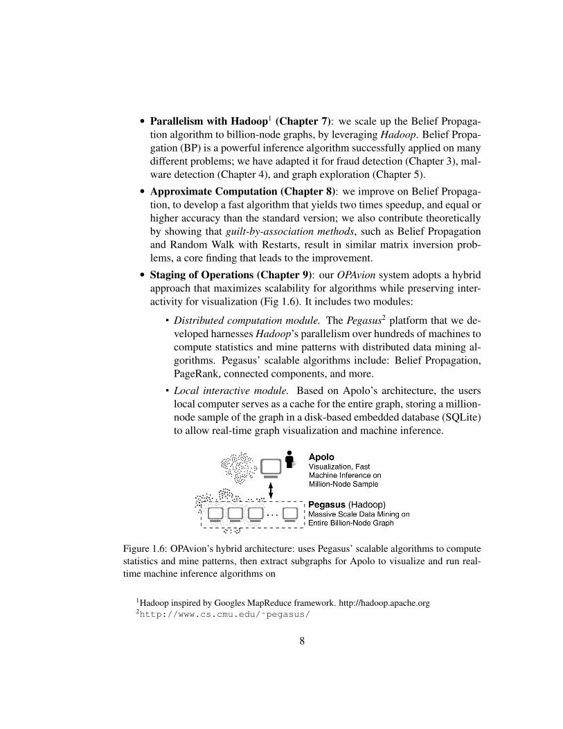
• Graphite (Chapter 6), a system that finds both exact and approximatematches for user-specified subgraphs. Sometimes, the user has some ideaabout the kind of subgraphs to look for, but is not able to describe it preciselyin words or in a computer language (e.g., SQL). Can we help the user eas-ily find patterns simply based on approximate descriptions? The Graphitesystem meets this challenge. It provides a direct-manipulation user inter-face for constructing the query pattern by placing nodes on the screen andconnecting them with edges (Fig 1.5).

6

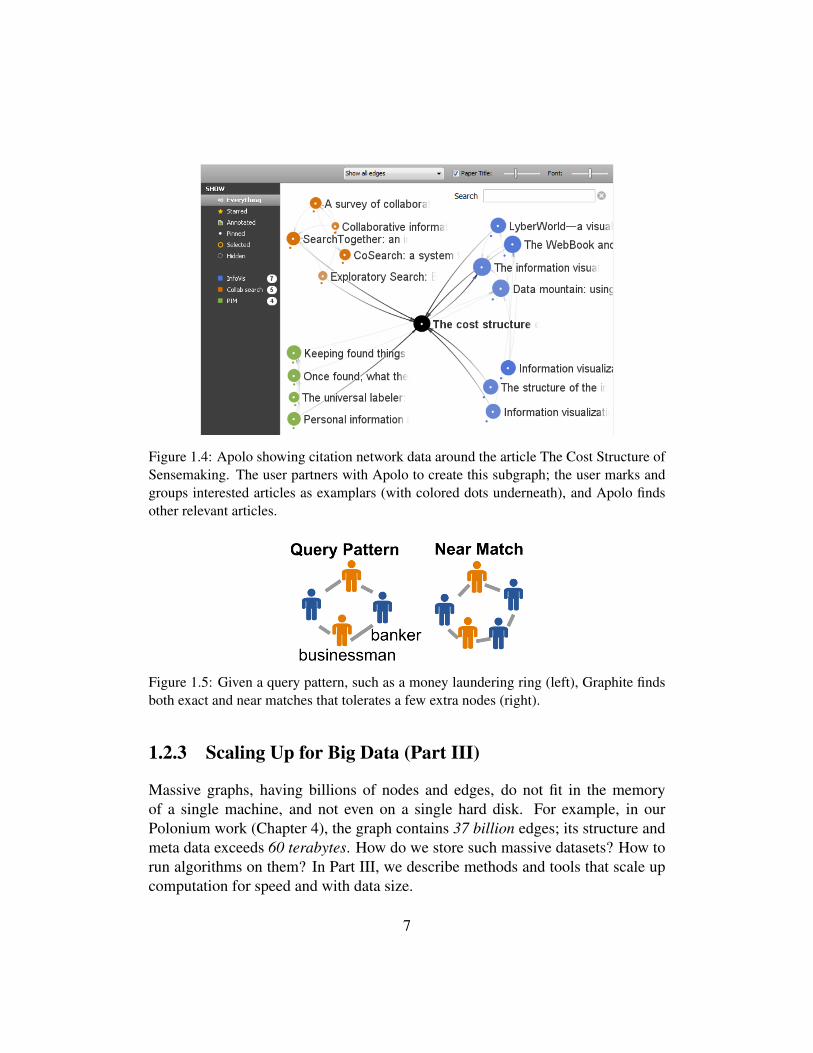
Figure 1.4: Apolo showing citation network data around the article The Cost Structure ofSensemaking. The user partners with Apolo to create this subgraph; the user marks andgroups interested articles as examplars (with colored dots underneath), and Apolo findsother relevant articles.

Figure 1.5: Given a query pattern, such as a money laundering ring (left), Graphite findsboth exact and near matches that tolerates a few extra nodes (right).

1.2.3 Scaling Up for Big Data (Part III)

Massive graphs, having billions of nodes and edges, do not fit in the memoryof a single machine, and not even on a single hard disk. For example, in ourPolonium work (Chapter 4), the graph contains 37 billion edges; its structure andmeta data exceeds 60 terabytes. How do we store such massive datasets? How torun algorithms on them? In Part III, we describe methods and tools that scale upcomputation for speed and with data size.

7

• Parallelism with Hadoop1 (Chapter 7): we scale up the Belief Propaga-tion algorithm to billion-node graphs, by leveraging Hadoop. Belief Propa-gation (BP) is a powerful inference algorithm successfully applied on manydifferent problems; we have adapted it for fraud detection (Chapter 3), mal-ware detection (Chapter 4), and graph exploration (Chapter 5).

• Approximate Computation (Chapter 8): we improve on Belief Propaga-tion, to develop a fast algorithm that yields two times speedup, and equal orhigher accuracy than the standard version; we also contribute theoreticallyby showing that guilt-by-association methods, such as Belief Propagationand Random Walk with Restarts, result in similar matrix inversion prob-lems, a core finding that leads to the improvement.

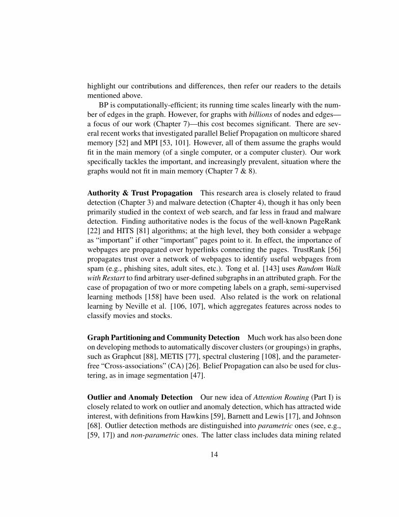
• Staging of Operations (Chapter 9): our OPAvion system adopts a hybridapproach that maximizes scalability for algorithms while preserving inter-activity for visualization (Fig 1.6). It includes two modules:

Distributed computation module. The Pegasus2 platform that we de-veloped harnesses Hadoop’s parallelism over hundreds of machines tocompute statistics and mine patterns with distributed data mining al-gorithms. Pegasus’ scalable algorithms include: Belief Propagation,PageRank, connected components, and more.

Local interactive module. Based on Apolo’s architecture, the userslocal computer serves as a cache for the entire graph, storing a million-node sample of the graph in a disk-based embedded database (SQLite)to allow real-time graph visualization and machine inference.

Figure 1.6: OPAvion’s hybrid architecture: uses Pegasus’ scalable algorithms to computestatistics and mine patterns, then extract subgraphs for Apolo to visualize and run real-time machine inference algorithms on

1Hadoop inspired by Googles MapReduce framework. http://hadoop.apache.org2http://www.cs.cmu.edu/˜pegasus/

8

1.3 Thesis Statement

We bridge Data Mining and Human-Computer Interaction (HCI) to synthesizenew methods and systems that help people understand and interact with massivegraphs with billions of nodes and edges, in three inter-related thrusts:

1. Attention Routing to funnel the users attention to the most interesting parts

2. Mixed-Initiative Sensemaking to guide the user’s exploration of the graph

3. Scaling Up by leveraging Hadoop’s parallelism, staging of operations, andapproximate computation

1.4 Big Data Mantra

This thesis advocates bridging Data Mining and HCI research to help researchersand practitioners to make sense of large graphs. We summarize our advocacy asthe CARDINAL mantra for big data3:

CARDINAL Mantra for Big DataMachine for Attention Routing, Human for Interaction

To elaborate, we suggest using machine (e.g., data mining, machine learn-ing) to help summarize big data and suggest potentially interesting starting pointsfor analysis; while the human interacts with these findings, visualizes them, andmakes sense of them using interactive tools that incorporate user feedback (e.g.,using machine learning) to help guide further exploration the data, form hypothe-ses, and develop a mental model about the data.

Designed to apply to analytics of large-scale data, we believe our mantra willnicely complement the conventional Visual Information-Seeking Mantra: “Overviewfirst, zoom and filter, then details-on-demand” which was originally proposed fordata orders of magnitude smaller [132].

We make explicit the needs to provide computation support throughout theanalytics process, such as using data mining techniques to help find interestingstarting points and route their attention there. We also highlight the importance

3CARDINAL is the acroynm for “Computerized Attention Routing in Data and InteractiveNavigation with Automated Learning”

9

that machine and human should work together—as partners—to make sense ofthe data and analysis results.

1.5 Research ContributionsThis thesis bridges data mining and HCI research. We contribute by answeringthree important, fundamental research questions in large graph analytics:• Where to start our analysis? Part I: Attention Routing• Where to go next? Part II: Mixed-Initiative Sensemaking• How to scale up? Part III: Scaling Up for Big DataWe concurrently contribute to multiple facets of data mining, HCI, and impor-

tantly, their intersection.

For Data Mining:• Algorithms: We design and develop a cohesive collection of algorithms

that scale to massive networks with billions of nodes and edges, such as Be-lief Propagation on Hadoop (Chapter 7), its faster version (Chapter 8), andgraph mining algorithms in Pegasus (http://www.cs.cmu.edu/˜pegasus).

• Systems: We contribute our scalable algorithms to the research commu-nity as the open-source Pegasus project, and interactive systems such asthe OPAvion system for scalable mining and visualization (Chapter 9), theApolo system for exploring large graph (Chapter 5), and the Graphite sys-tem for matching user-specified subgraph patterns (Chapter 6).

• Theories: We present theories that unify graph mining approaches (e.g.,random walk with restart, belief propagation, semi-supervised learning),which enable us to make algorithms even more scalable (Chapter 8).

• Applications: Inspired by graph mining research, we formulate and solveimportant real-world problems with ideas, solutions, and implementationsthat are first of their kinds. We tackled problems such as detecting auctionfraudsters (Chapter 3) and unearthing malware (Chapter 4).

For HCI:• New Class of InfoVis Methods: Our Attention Routing idea (Part I) adds

a new class of nontrivial methods to information visualization, as a viableresource for the critical first step of locating starting points for analysis.

10

• New Analytics Paradigm: Apolo (Chapter 5) represents a paradigm shiftin interactive graph analytics. It enables users to evolve their mental modelsof the graph in a bottom-up manner (analogous to the constructivist view inlearning), by starting small, rather starting big and drilling down, offering asolution to the common phenomena that there are simply no good ways topartition most massive graphs to create visual overviews.

• Scalable Interactive Tools: Our interactive tools (e.g., Apolo, Graphite)advances the state of the art, by enabling people to interact with graphsorders of magnitudes larger in real time (tens of millions of edges).

This thesis research opens up opportunities for a new breed of systems andmethods that combine HCI and data mining methods to enable scalable, interac-tive analysis of big data. We hope that our thesis, and our big data mantra “Ma-chine for Attention Routing, Human for Interaction” will serve as the catalyst thataccelerates innovation across these disciplines, and the bridge that connects them.inspiring more researchers and practitioners to work together at the crossroad ofData Dining and HCI.

1.6 ImpactThis thesis work has made remarkable impact to society:• Our Polonium technology (Chapter 4), fully integrated into Symantec’s

flagship Norton Antivirus products, protects 120 million people worldwidefrom malware, and has answered over trillions of queries for file reputationqueries. Polonium is patent-pending.

• Our NetProbe system (Chapter 3), which fingers fraudsters on eBay, madeheadlines in major media outlets, like Wall Street Journal, CNN, and USAToday. Interested by our work, eBay invited us for a site visit and presenta-tion.

• Our Pegasus project (Chapter 7 & 9), which creates scalable graph algo-rithms, won the Open Source Software World Challenge, Silver Award. Wehave released Pegasus as free, open-source software, downloaded by peoplefrom over 83 countries. It is also part of Windows Azure, Microsoft’s cloudcomputing platform.

• Apolo (Chapter 5), as a major visualization component, contributes to DARPA’sAnomaly Detection at Multiple Scales project (ADAMS) to detect insiderthreats and exfiltration in government and the military.

11

12

Chapter 2

Literature Survey

Our survey focuses on three inter-related areas from which our thesis contributesto: (1) graph mining algorithms and tools; (2) graph visualization and exploration;and (3) sensemaking.

2.1 Graph Mining Algorithms and Tools

Inferring Node Relevance A lot of research in graph mining studies how tocompute relevance between two nodes in a network; many of them belong tothe class of spreading-activation [13] or propagation-based algorithms, e.g., HITS[81], PageRank [22], and random walk with restart [144].

Belief Propagation (BP) [155] is an efficient inference algorithm for prob-abilistic graphical models. Originally proposed for computing exact marginaldistributions for trees [117], it was later applied on general graphs [118] as anapproximate algorithm. When the graph contains loops, it’s called loopy BP.

Since its proposal, BP has been widely and successfully used in a myriadof domains to solve many important problems, such as in error-correcting codes(e.g., Turbo code that approaches channel capacity), computer vision (for stereoshape estimation and image restoration [47]), and pinpointing misstated accountsin general ledger data for the financial domain [98].

We have adapted it for fraud detection (Chapters 3), malware detection (Chap-ters 4) and sensemaking (Chapters 5), and provides theories (Chapters 8) and im-plementations (Chapters 7) that make it scale to massive graphs. We describeBP’s details in Section 3.3, in the context of NetProbe’s auction fraud detectionproblem. Later, in other works where we adapt or improve BP, we will briefly

13

highlight our contributions and differences, then refer our readers to the detailsmentioned above.

BP is computationally-efficient; its running time scales linearly with the num-ber of edges in the graph. However, for graphs with billions of nodes and edges—a focus of our work (Chapter 7)—this cost becomes significant. There are sev-eral recent works that investigated parallel Belief Propagation on multicore sharedmemory [52] and MPI [53, 101]. However, all of them assume the graphs wouldfit in the main memory (of a single computer, or a computer cluster). Our workspecifically tackles the important, and increasingly prevalent, situation where thegraphs would not fit in main memory (Chapter 7 & 8).

Authority & Trust Propagation This research area is closely related to frauddetection (Chapter 3) and malware detection (Chapter 4), though it has only beenprimarily studied in the context of web search, and far less in fraud and malwaredetection. Finding authoritative nodes is the focus of the well-known PageRank[22] and HITS [81] algorithms; at the high level, they both consider a webpageas “important” if other “important” pages point to it. In effect, the importance ofwebpages are propagated over hyperlinks connecting the pages. TrustRank [56]propagates trust over a network of webpages to identify useful webpages fromspam (e.g., phishing sites, adult sites, etc.). Tong et al. [143] uses Random Walkwith Restart to find arbitrary user-defined subgraphs in an attributed graph. For thecase of propagation of two or more competing labels on a graph, semi-supervisedlearning methods [158] have been used. Also related is the work on relationallearning by Neville et al. [106, 107], which aggregates features across nodes toclassify movies and stocks.

Graph Partitioning and Community Detection Much work has also been doneon developing methods to automatically discover clusters (or groupings) in graphs,such as Graphcut [88], METIS [77], spectral clustering [108], and the parameter-free “Cross-associations” (CA) [26]. Belief Propagation can also be used for clus-tering, as in image segmentation [47].

Outlier and Anomaly Detection Our new idea of Attention Routing (Part I) isclosely related to work on outlier and anomaly detection, which has attracted wideinterest, with definitions from Hawkins [59], Barnett and Lewis [17], and Johnson[68]. Outlier detection methods are distinguished into parametric ones (see, e.g.,[59, 17]) and non-parametric ones. The latter class includes data mining related

14

methods such as distance-based and density-based methods. These methods typ-ically define as an outlier the (n-D) point that is too far away from the rest, andthus lives in a low-density area [83]. Typical methods include LOF [21] and LOCI[115], with numerous variations: [32, 9, 14, 55, 109, 157, 78].

Noble and Cook [110] detect anomalous sub-graphs. Eberle and Holder [44]try to spot several types of anomalies (like unexpected or missing edges or nodes).Chakrabarti [25] uses MDL (Minimum Description Language) to spot anomalousedges, while Sun et al. [136] use proximity and random walks to spot anomaliesin bipartite graphs.

Graph Pattern Matching Some of our work concerns matching patterns (sub-graphs) in large graphs, such as our NetProbe system (Chapter 3) which detectssuspicious near-bipartite cores formed among fraudsters’ transcations in onlineauction, and our Graphite system (Chapter 6) which finds user-specified subgraphsin large attributed graphs using best effort, and returns exact and near matches.

Graph matching algorithms vary widely due to differences in the specific prob-lems they address. The survey by Gallagher [50] provides an excellent overview.Yan, Yu, and Han proposed efficient methods for indexing [153] and mining graphdatabases for frequent subgraphs (e.g., gSpan [152]). Jin et al. used the concept oftopological minor to discover frequent large patterns [67]. These methods weredesigned for graph-transactional databases, such as collections of biological orchemical structures; while our work (Graphite) detects user-specified pattern ina single-graph setting by extending the ideas of connection subgraphs [46] andcenterpiece graphs [142]. Other related systems include the GraphMiner system[148] and works such as [119, 154].

Large Graph Mining with MapReduce and Hadoop Large scale graph min-ing poses challenges in dealing with massive amount of data. One might considerusing a sampling approach to decrease the amount of data. However, samplingfrom a large graph can lead to multiple nontrivial problems that do not have sat-isfactory solutions [92]. For example, which sampling methods should we use?Should we get a random sample of the edges, or the nodes? Both options havetheir own share of problems: the former gives poor estimation of the graph diam-eter, while the latter may miss high-degree nodes.

A promising alternative for large graph mining is MAPREDUCE, a parallelprogramming framework [39] for processing web-scale data. MAPREDUCE hastwo advantages: (a) The data distribution, replication, fault-tolerance, load bal-

15

ancing is handled automatically; and furthermore (b) it uses the familiar conceptof functional programming. The programmer defines only two functions, a mapand a reduce. The general framework is as follows [89]: (a) the map stage readsthe input file and emits (key, value) pairs; (b) the shuffling stage sorts the outputand distributes them to reducers; (c) the reduce stage processes the values withthe same key and emits another (key, value) pairs which become the final result.

HADOOP [2] is the open source version of MAPREDUCE. Our work (Chapter7, 8, 9) leverages it to scale up graph mining tasks. HADOOP uses its own dis-tributed file system HDFS, and provides a high-level language called PIG [111].Due to its excellent scalability and ease of use, HADOOP is widely used for largescale data mining, as in [116], [74], [72], and in our Pegasus open-source graphlibrary [75]. Other variants which provide advanced MAPREDUCE-like systemsinclude SCOPE [24], Sphere [54], and Sawzall [121].

2.2 Graph Visualization and ExplorationThere is a large body of research aimed at understanding and supporting howpeople can gain insights through visualization [87]. Herman et al [62] present asurvey of techniques for visualizing and navigating graphs, discussing issues re-lated to layout, 2D versus 3D representations, zooming, focus plus context views,and clustering. It is important to note, however, that the graphs that this surveyexamines are on the order of hundreds or thousands of nodes, whereas we areinterested in graphs of several orders of magnitude larger in size.

Systems and Libraries There are well-known visualization systems and soft-ware libraries, such as Graphviz [1], Walrus [6], Otter [4], Prefuse [61, 5], JUNG[3], but they only perform graph layout, without any functionality for outlier de-tection and sensemaking. Similarly, interactive visualization systems, such as Cy-toscape [131], GUESS [8], ASK-GraphView [7], and CGV [141] only supportgraphs with orders of magnitude smaller than our target scale, and assume ana-lysts would perform their analysis manually, which can present great challenge forhuge graphs. Our work differs by offering algorithmic support to guide analyststo spot patterns, and form hypotheses and verify them, all at a much larger scale.

Supporting “Top-down” Exploration A number of tools have been developedto support “landscape” views of information. These include WebBook and Web-Forager [23], which use a book metaphor to find, collect, and manage web pages;

16

Butterfly [94] aimed at accessing articles in citation networks; and Webcutter,which collects and presents URL collections in tree, star, and fisheye views [93].For a more focused review on research visualizing bibliographic data, see [99].

Supporting “Bottom-up” Exploration In contrast to many of these systemswhich focus on providing overviews of information landscapes, less work hasbeen done on supporting the bottom-up sensemaking approach [128] aimed athelping users construct their own landscapes of information. Our Apolo system(Chapter 5) was designed to help fill in this gap. Some research has started tostudy how to support local exploration of graphs, including Treeplus [90], Vizster[60], and the degree-of-interest approach proposed in [146]. These approachesgenerally support the idea of starting with a small subgraph and expanding nodesto show their neighborhoods (and in the case of [146], help identify useful neigh-borhoods to expand). One key difference with these works is that Apolo changesthe very structure of the expanded neighborhoods based on users’ interactions,rather than assuming the same neighborhoods for all users.

2.3 SensemakingSensemaking refers to the iterative process of building up a representation of aninformation space that is useful for achieving the user’s goal [128]. Some of ourwork is specifically designed to help people make sense of large graph data, suchas our Apolo system (Chapter 5) which combines machine learning, visualizationand interaction to guide the user to explore large graphs.

Models and Tools Numerous sensemaking models have been proposed, includ-ing Russell et al.’s cost structure view [128], Dervin’s sensemaking methodology[40], and the notional model by Pirolli and Card [122]. Consistent with this dy-namic task structure, studies of how people mentally learn and represent conceptshighlight that they are often flexible, ad-hoc, and theory-driven rather than deter-mined by static features of the data [18]. Furthermore, categories that emerge inusers’ minds are often shifting and ad-hoc, evolving to match the changing goalsin their environment [79].

These results highlight the importance of a “human in the loop” approach (thefocus of Part II) for organizing and making sense of information, rather than fullyunsupervised approaches that result in a common structure for all users. Sev-eral systems aim to support interactive sensemaking, like SenseMaker [16], Scat-

17

ter/Gather [38], Russell’s sensemaking systems for large document collections[127], Jigsaw [135], and Analyst’s Notebook [82]. Other relevant approaches in-clude [139] and [12] which investigated how to construct, organize and visualizetopically related web resources.

Integrating Graph Mining In our Apolo work (Chapter 5), we adapts BeliefPropagation to support sensemaking, because of its unique capability to simulta-neous support: multiple user-specified exemplars (unlike [146]); any number ofgroups (unlike [13, 69, 146]); linear scalability with the number of edges (bestpossible for most graph algorithms); and soft clustering, supporting membershipin multiple groups.

There has been few tools like ours that have integrated graph algorithms tointeractively help people make sense of network information [69, 120, 146], andthey often only support some of the desired sensemaking features, e.g., [146]supports one group and a single exemplar.

18

Part I

Attention Routing

19

Overview

A fundamental problem in analyzing large graphs is that there are simply notenough pixels on the screen to show the entire graph. Even if there were, largegraphs appear as incomprehensible blobs (as in Fig 1.1).

Attention Routing is a new idea we introduced to overcome this critical prob-lem in visual analytics, to help users locate good starting points for analysis.Based on anomaly detection in data mining, attention routing methods channelusers’ attention through massive networks to interesting nodes or subgraphs thatdo not conform to normal behavior.

Conventionally, the mantra “overview first, zoom & filter, details-on-demand”in information visualization relies solely on people’s perceptual ability to manu-ally find starting points for analysis. Attention routing adds a new class of non-trivial methods provide computation support to this critical first step. In this part,we will describe several attention routing tools.• NetProbe (Chapter 3) fingers bad guys in online auction by identifying

their suspicious transactions that form near-bipartite cores.• Polonium (Chapter 4) unearths malware among 37 billion machine-file

relationships.

20

Chapter 3

NetProbe: Fraud Detection inOnline Auction

This chapter describes our first example of Attention Routing, which finds fraud-ulent users and their suspicious transaction in online auctions. These users andtransactions formed some special signature subgraphs called near-bipartite cores(as we will explain), which can serve as excellent starting points for fraud analysts.

We describe the design and implementation of NetProbe, a system that modelsauction users and transactions as a Markov Random Field tuned to detect the suspi-cious patterns that fraudsters create, and employs a Belief Propagation mechanismto detect likely fraudsters. Our experiments show that NetProbe is both efficientand effective for fraud detection. We report experiments on synthetic graphs withas many as 7,000 nodes and 30,000 edges, where NetProbe was able to spot fraud-ulent nodes with over 90% precision and recall, within a matter of seconds. Wealso report experiments on a real dataset crawled from eBay, with nearly 700,000transactions between more than 66,000 users, where NetProbe was highly effec-tive at unearthing hidden networks of fraudsters, within a realistic response timeof about 6 minutes. For scenarios where the underlying data is dynamic in na-ture, we propose Incremental NetProbe, which is an approximate, but fast, variantof NetProbe. Our experiments prove that Incremental NetProbe executes nearlydoubly fast as compared to NetProbe, while retaining over 99% of its accuracy.

Chapter adapted from work appeared at WWW 2007 [114]

21

3.1 Introduction

Online auctions have been thriving as a business over the past decade. Peoplefrom all over the world trade goods worth millions of dollars every day usingthese virtual marketplaces. EBay (www.ebay.com), the world’s largest auctionsite, reported a third quarter revenue of $1,449 billion, with over 212 million reg-istered users [42]. These figures represent a 31% growth in revenue and 26%growth in the number of registered users over the previous year. Unfortunately,rapid commercial success has made auction sites a lucrative medium for commit-ting fraud. For more than half a decade, auction fraud has been the most prevalentInternet crime. Auction fraud represented 63% of the complaints received by theFederal Internet Crime Complaint Center last year. Among all the monetary lossesreported, auction fraud accounted for 41%, with an average loss of $385 [65].

Despite the prevalence of auction frauds, auctions sites have not come up withsystematic approaches to expose fraudsters. Typically, auction sites use a reputa-tion based framework for aiding users to assess the trustworthiness of each other.However, it is not difficult for a fraudster to manipulate such reputation systems.As a result, the problem of auction fraud has continued to worsen over the past

. . . . . . . . .

Application ServerRuns algorithms to spot suspicious

patterns in auction graph.

Crawler Agents2-tier parallelizable. Multiple agents with multiple threads

to download auction data.

Data Master Maintain centralized queue to

avoid redundant crawlling.

User Queries Trustworthiness of "Alisher"User enters the user ID "Alisher" into a Java applet that talks to the server, which sends assessment results in an XML file.

The applet interprets and visualizes suspicious networks.

Online Auction SiteAuction data modelled as graphNodes: usersEdges: transactions

. . .

XML

NetProbe

Figure 3.1: Overview of the NetProbe system

22

few years, causing serious concern to auction site users and owners alike.We therefore ask ourselves the following research questions - given a large

online auction network of auction users and their histories of transactions, howdo we spot fraudsters? How should we design a system that will carry out frauddetection on auction sites in a fast and accurate manner?

We propose NetProbe a system for fraud detection in online auction sites (Fig-ure 3.1). NetProbe is a system that systematically analyzes transactions withinusers of auction sites to identify suspicious networks of fraudsters. NetProbe al-lows users of an online auction site to query the trustworthiness of any other user,and offers an interface to visually explains the query results. In particular, wemake the following contributions through NetProbe:

• First, we propose data models and algorithms based on Markov RandomFields and belief propagation to uncover suspicious networks hidden withinan auction site. We also propose an incremental version of NetProbe whichperforms almost twice as fast in dynamic environments, with negligible lossin accuracy.

• Second, we demonstrate that NetProbe is fast, accurate, and scalable, withexperiments on large synthetic and real datasets. Our synthetic datasets con-tained as many as 7,000 users with over 30,000 transactions, while the realdataset (crawled from eBay) contains over 66,000 users and nearly 800,000transactions.

• Lastly, we share the non-trivial design and implementation decisions thatwe made while developing NetProbe. In particular, we discuss the follow-ing contributions: (a) a parallelizable crawler that can efficiently crawl datafrom auction sites, (b) a centralized queuing mechanism that avoids redun-dant crawling, (c) fast, efficient data structures to speed up our fraud de-tection algorithm, and (d) a user interface that visually demonstrates thesuspicious behavior of potential fraudsters to the end user.

The rest of this work is organized as follows. We begin by reviewing relatedwork in Section 3.2. Then, we describe the algorithm underlying NetProbe inSection 3.3 and explain how it uncovers dubious associations among fraudsters.We also discuss the incremental variant of NetProbe in this section. Next, in Sec-tion 3.4, we report experiments that evaluate NetProbe (as well as its incrementalvariant) on large real and synthetic datasets, demonstrating NetProbe’s effective-ness and scalability. In Section 3.5, we describe NetProbe’s full system design andimplementation details. Finally, we summarize our contributions in Section 3.6and outline directions for future work.

23

3.2 Related WorkIn this section, we survey related approaches for fraud detection in auction sites,as well as the literature on reputation systems that auction sites typically use toprevent fraud. We also look at related work on trust and authority propagation, andgraph mining, which could be applied to the context of auction fraud detection.

3.2.1 Grass-Roots EffortsIn the past, attempts have been made to help people identify potential fraudsters.However, most of them are “common sense” approaches, recommended by avariety of authorities such as newspapers articles [145], law enforcement agen-cies [49], or even from auction sites themselves [43]. These approaches usuallysuggest that people be cautious at their end and perform background checks ofsellers that they wish to transact with. Such suggestions however, require users tomaintain constant vigilance and spend a considerable amount of time and effort ininvestigating potential dealers before carrying out a transaction.

To overcome this difficulty, self-organized vigilante organizations are formed,usually by auction fraud victims themselves, to expose fraudsters and report themto law enforcement agencies [15]. Unfortunately, such grassroot efforts are in-sufficient for regulating large-scale auction fraud, motivating the need for a moresystematic approach to solve the auction fraud problem.

3.2.2 Auction Fraud and Reputation SystemsReputation systems are used extensively by auction sites to prevent fraud. Butthey are usually very simple and can be easily foiled. In an overview, Resnick etal. [124] summarized that modern reputation systems face many challenges whichinclude the difficulty to elicit honest feedback and to show faithful representationsof users’ reputation. Despite their limitations, reputation systems have had a sig-nificant effect on how people buy and sell. Melnik et al. [100] and Resnick etal. [125] conducted empirical studies which showed that selling prices of goodsare positively affected by the seller’s reputation, implying people feel more con-fident to buy from trustworthy sources. In summary, reputation systems mightnot be an effective mechanism to prevent fraud because fraudsters can easily trickthese systems to manipulating their own reputation.

Chua et al. [37] have categorized auction fraud into different types, but theydid not formulate methods to combat them. They suggest that an effective ap-

24

proach to fight auction fraud is to allow law enforcement and auction sites to joinforces, which can be costly from both monetary and managerial perspectives.

In our previous work, we explored a classification-based fraud detectionscheme [29]. We extracted features from auction data to capture fluctuations insellers’ behaviors (e.g., selling numerous expensive items after selling very fewcheap items). This method, though promising, warranted further enhancement be-cause it did not take into account the patterns of interaction employed by fraudsterswhile dealing with other auction users. To this end, we suggested a fraud detec-tion algorithm by identifying suspicious networks amongst auction site users [31].However, the experiments were reported over a tiny dataset, while here we reportan in-depth evaluation over large synthetic and real datasets, along with fast, in-cremental computation techniques.

3.3 NetProbe: Proposed AlgorithmsIn this section, we present NetProbe’s algorithm for detecting networks of fraud-sters in online auctions. The key idea is to infer properties for a user based onproperties of other related users. In particular, given a graph representing interac-tions between auction users, the likelihood of a user being a fraudster is inferredby looking at the behavior of its immediate neighbors . This mechanism is ef-fective at capturing fraudulent behavioral patterns, and affords a fast, scalableimplementation (see Section 3.4).

We begin by describing the Markov Random Field (MRF) model, which is apowerful way to model the auction data in graphical form. We then describe theBelief Propagation algorithm, and present how NetProbe uses it for fraud detec-tion. Finally, we present an incremental version of NetProbe which is a quick andaccurate way to update beliefs when the graph topology changes.

3.3.1 The Markov Random Field ModelMRFs are a class of graphical models particularly suited for solving inferenceproblems with uncertainty in observed data. MRFs are widely used in imagerestoration problems wherein the observed variables are the intensities of eachpixel in the image, while the inference problem is to identify high-level detailssuch as objects or shapes.

A MRF consists of an undirected graph, each node of which can be in any of afinite number of states. The state of a node is assumed to statistically depend only

25

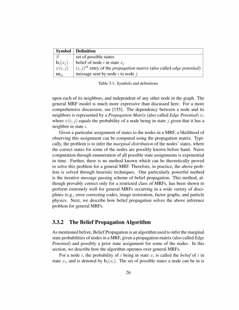
Symbol DefinitionS set of possible statesbi(xj) belief of node i in state xjψ(i, j) (i, j)th entry of the propagation matrix (also called edge potential)mij message sent by node i to node j

Table 3.1: Symbols and definitions

upon each of its neighbors, and independent of any other node in the graph. Thegeneral MRF model is much more expressive than discussed here. For a morecomprehensive discussion, see [155]. The dependency between a node and itsneighbors is represented by a Propagation Matrix (also called Edge Potential) ψ,where ψ(i, j) equals the probability of a node being in state j given that it has aneighbor in state i.

Given a particular assignment of states to the nodes in a MRF, a likelihood ofobserving this assignment can be computed using the propagation matrix. Typi-cally, the problem is to infer the marginal distribution of the nodes’ states, wherethe correct states for some of the nodes are possibly known before hand. Naivecomputation through enumeration of all possible state assignments is exponentialin time. Further, there is no method known which can be theoretically provedto solve this problem for a general MRF. Therefore, in practice, the above prob-lem is solved through heuristic techniques. One particularly powerful methodis the iterative message passing scheme of belief propagation. This method, al-though provably correct only for a restricted class of MRFs, has been shown toperform extremely well for general MRFs occurring in a wide variety of disci-plines (e.g., error correcting codes, image restoration, factor graphs, and particlephysics. Next, we describe how belief propagation solves the above inferenceproblem for general MRFs.

3.3.2 The Belief Propagation Algorithm

As mentioned before, Belief Propagation is an algorithm used to infer the marginalstate probabilities of nodes in a MRF, given a propagation matrix (also called EdgePotential) and possibly a prior state assignment for some of the nodes. In thissection, we describe how the algorithm operates over general MRFs.

For a node i, the probability of i being in state xi is called the belief of i instate xi, and is denoted by bi(xi). The set of possible states a node can be in is

26

Figure 3.2: A sample execution of NetProbe. Red triangles: fraudulent, yellow diamonds:accomplice, white ellipses: honest, gray rounded rectangles: unbiased.

represented by S. Table 3.1 lists the symbols and their definitions used in thissection.

At the high level, the algorithm infers a node’s label from some prior knowl-edge about the node, and from the node’s neighbors through iterative messagepassing between all pairs of node i and j.

Node i’s prior is specified using the node potential function φ(xi)1. And a

message mij(xj) sent from node i to j intuitively represents i’s opinion about j’sbelief (i.e., its distribution). An outgoing message from node i is generated basedon the messages going into the node; in other words, a node aggregates and trans-forms its neighbors’ opinions about itself into an outgoing opinion that the nodewill exert on its neighbors. The transformation is specified by the propagationmatrix (also called edge potential function) ψij (xi, xj), which formally describesthe probability of a node i being in class xi given that its neighbor j is in class xj .Mathematically, a message is computed as:

1In case there is no prior knowledge available, each node is initialized to an unbiased state (i.e.,it is equally likely to be in any of the possible states), and the initial messages are computed bymultiplying the propagation matrix with these initial, unbiased beliefs.

27

mij (xj) =∑xi∈X

φ (xi)ψij (xi, xj)∏

k∈N(i)\j

mki (xi) (3.1)

where mij : the message vector sent by node i to jN(i) \ j : node i’s neighbors, excluding node j

c : normalization constantAt any time, a node’s belief can be computed by multiplying its prior with all

the incoming messages (c is a normalizing constant):

bi (xi) = cφ (xi)∏

j∈N(i)

mji (xi) (3.2)

The algorithm is typically stopped when the beliefs converge (within somethreshold; 10−5 is commonly used), or after some number of iterations. Althoughconvergence is not guaranteed theoretically for general graphs (except for trees),the algorithm often converges quickly in practice.

3.3.3 NetProbe for Online AuctionsWe now describe how NetProbe utilizes the MRF modeling to solve the frauddetection problem.

Transactions between users are modeled as a graph, with a node for each userand an edge for one (or more) transactions between two users. As is the case withhyper-links on the Web (where PageRank [22] posits that a hyper-link confersauthority from the source page to the target page), an edge between two nodesin an auction network can be assigned a definite semantics, and can be used topropagate properties from one node to its neighbors. For instance, an edge can beinterpreted as an indication of similarity in behavior — honest users will interactmore often with other honest users, while fraudsters will interact in small cliquesof their own (to mutually boost their credibility). This semantics is very similar inspirit to that used by TrustRank [56], a variant of PageRank used to combat Webspam. Under this semantics, honesty/fraudulence can be propagated across edgesand consequently, fraudsters can be detected by identifying relatively small anddensely connected subgraphs (near cliques).

However, our previous work [31] suggests that fraudsters do not form suchcliques. There are several reasons why this might be so:• Auction sites probably use techniques similar to the one outlined above to

detect probable fraudsters and void their accounts.

28

• Once a fraud is committed, an auction site can easily identify and void theaccounts of other fraudsters involved in the clique, destroying the “infras-tructure” that the fraudster had invested in for carrying out the fraud. Tocarry out another fraud, the fraudster will have to re-invest efforts in build-ing a new clique.

Instead, we uncovered a different modus operandi for fraudsters in auctionnetworks, which leads to the formation of near bipartite cores. Fraudsters createtwo types of identities and arbitrarily split them into two categories – fraud andaccomplice. The fraud identities are the ones used eventually to carry out theactual fraud, while the accomplices exist only to help the fraudsters carry outtheir job by boosting their feedback rating. Accomplices themselves behave likeperfectly legitimate users and interact with other honest users to achieve highfeedback ratings. On the other hand, they also interact with the fraud identitiesto form near bipartite cores, which helps the fraud identities gain a high feedbackrating. Once the fraud is carried out, the fraud identities get voided by the auctionsite, but the accomplice identities linger around and can be reused to facilitate thenext fraud.

We model the auction users and their mutual transactions as a MRF. A nodein the MRF represents a user, while an edge between two nodes denotes that thecorresponding users have transacted at least once. Each node can be in any of 3states — fraud, accomplice, and honest.

To completely define the MRF, we need to instantiate the propagation matrix.Recall that an entry in the propagation matrix ψ(xj, xi) gives the likelihood of anode being in state xi given that it has a neighbor in state xj . A sample instantia-tion of the propagation matrix is shown in Table 3.2. This instantiation is based onthe following intuition: a fraudster tends to heavily link to accomplices but avoidslinking to other bad nodes; an accomplice tends to link to both fraudsters andhonest nodes, with a higher affinity for fraudsters; a honest node links with otherhonest nodes as well as accomplices (since an accomplice effectively appears tobe honest to the innocent user.) In our experiments, we set εp to 0.05. Automati-cally learning the correct value of εp as well as the form of the propagation matrixitself would be valuable future work.

3.3.4 NetProbe: A Running Example

In this section, we present a running example of how NetProbe detects bipartitecores using the propagation matrix in Table 3.2. Consider the graph shown in

29

Node stateNeighbor state Fraud Accomplice HonestFraud εp 1− 2εp εpAccomplice 0.5 2εp 0.5− 2εpHonest εp (1− εp)/2 (1− εp)/2

Table 3.2: Instantiation of the propagation matrix for fraud detection. Entry (i, j) denotesthe probability of a node being in state j given that it has a neighbor in state i.

Figure 3.2. The graph consists of a bipartite core (nodes 7, 8, . . . , 14) mingledwithin a larger network. Each node is encoded to depict its state — red trianglesindicate fraudsters, yellow diamonds indicate accomplices, white ellipses indicatehonest nodes, while gray rounded rectangles indicate unbiased nodes (i.e., nodesequally likely to be in any state.)

Each node is initialized to be unbiased, i.e., it is equally likely to be fraud,accomplice or honest. The nodes then iteratively pass messages and affect eachother’s beliefs. Notice that the particular form of the propagation matrix we useassigns a higher chance of being an accomplice to every node in the graph atthe end of the first iteration. These accomplices then force their neighbors to befraudsters or honest depending on the structure of the graph. In case of bipartitecores, one half of the core is pushed towards the fraud state, leading to a stableequilibrium. In the remaining graph, a more favorable equilibrium is achieved bylabeling some of the nodes as honest.

At the end of execution, the nodes in the bipartite core are neatly labeled asfraudsters and accomplices. The key idea is the manner in which accomplicesforce their partners to be fraudsters in bipartite cores, thus providing a good mech-anism for their detection.

3.3.5 Incremental NetProbeIn a real deployment of NetProbe, the underlying graph corresponding to transac-tions between auction site users, would be extremely dynamic in nature, with newnodes (i.e., users) and edges (i.e., transactions) being added to it frequently. Insuch a setting, if one expects an exact answer from the system, NetProbe wouldhave to propagate beliefs over the entire graph for every new node/edge that getsadded to the graph. This would be infeasible in systems with large graphs, andespecially for online auction sites where users expect interactive response times.

Intuitively, the addition of a few edges to a graph should not perturb the re-

30

Figure 3.3: An example of Incremental NetProbe. Red triangles: fraudulent, yellow di-amonds: accomplice, white ellipses: honest. An edge is added between nodes 9 and 10of the graph on the left. Normal propagation of beliefs in the 3-vicinity of node 10 (onthe right) leads to incorrect inference, and so nodes on the boundary of the 3-vicinity (i.e.node 6) should retain their beliefs.

31

maining graph by a lot (especially disconnected components.) To avoid wastefulrecomputation of node beliefs from scratch, we developed a mechanism to incre-mentally update beliefs of nodes upon small changes in the graph structure. Werefer to this variation of our system as Incremental NetProbe.

The motivation behind Incremental NetProbe is that addition of a new edgewill at worst result in minor changes in the immediate neighborhood of the edge,while the effect will not be strong enough to propagate to the rest of the graph.Whenever a new edge gets added to the graph, the algorithm proceeds by per-forming a breadth-first search of the graph from one of the end points (call it n)of the new edge, up to a fixed number of hops h, so as to retrieve a small sub-graph, which we refer to as the h-vicinity of n. It is assumed that only the beliefsof nodes within the h-vicinity are affected by addition of the new edge. Then,“normal” belief propagation is performed only over the h-vicinity, with one keydifference. While passing messages between nodes, beliefs of the nodes on theboundary of the h-vicinity are kept fixed to their original values. This ensuresthat the belief propagation takes into account the global properties of the graph,in addition to the local properties of the h-vicinity.

The motivation underlying Incremental NetProbe’s algorithm is exemplifiedin Figure 3.3. The initial graph is shown on the left hand side, to which an edgeis added between nodes 9 and 10. The 3-vicinity of node 10 is shown on the righthand side. The nodes on the right hand side are colored according to their inferredstates based on propagating beliefs only in the subgraph without fixing the beliefof node 6 to its original value. Note that the 3-vicinity does not capture the fact thatnode 6 is a part of a bipartite core. Hence the beliefs inferred are influenced onlyby the local structure of the 3-vicinity and are “out of sync” with the remaininggraph. In order to make sure that Incremental NetProbe retains global propertiesof the graph, it is essential to fix the beliefs of nodes at the boundary of the 3-vicinity to their original values.

3.4 EvaluationWe evaluated the performance of NetProbe over synthetic as well as real datasets.Overall, NetProbe was effective – it detected bipartite cores with very high ac-curacy – as well as efficient – it had fast execution times. We also conductedpreliminary experiments with Incremental NetProbe, which indicate that Incre-mental NetProbe results in significant speed-up of execution time with negligibleloss of accuracy.

32

0

0.2

0.4

0.6

0.8

1

1.2

100 600 1100 1600 2100 2600

#nodes

RecallPrecision

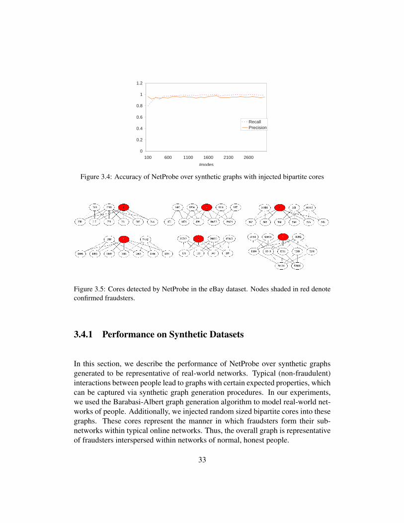
Figure 3.4: Accuracy of NetProbe over synthetic graphs with injected bipartite cores

Figure 3.5: Cores detected by NetProbe in the eBay dataset. Nodes shaded in red denoteconfirmed fraudsters.

3.4.1 Performance on Synthetic Datasets

In this section, we describe the performance of NetProbe over synthetic graphsgenerated to be representative of real-world networks. Typical (non-fraudulent)interactions between people lead to graphs with certain expected properties, whichcan be captured via synthetic graph generation procedures. In our experiments,we used the Barabasi-Albert graph generation algorithm to model real-world net-works of people. Additionally, we injected random sized bipartite cores into thesegraphs. These cores represent the manner in which fraudsters form their sub-networks within typical online networks. Thus, the overall graph is representativeof fraudsters interspersed within networks of normal, honest people.

33

0

200

400

600

800

1000

1200

1400

1600

0 5000 10000 15000 20000 25000 30000

#edges

tim

e (m

s)

Figure 3.6: Scalability of NetProbe over synthetic graphs

3.4.2 Accuracy of NetProbe

We ran NetProbe over synthetic graphs of varying sizes. and measured the ac-curacy of NetProbe in detecting bipartite cores via precision and recall. In ourcontext, precision is the fraction of nodes labeled by NetProbe as fraudsters whobelonged to a bipartite core, while recall is the fraction of nodes belonging to abipartite core that were labeled by NetProbe as fraudsters. The results are areplotted in Figure 3.4.

In all cases, recall is very close to 1, which implies that NetProbe detectsalmost all bipartite cores. Precision is almost always above 0.9, which indicatesthat NetProbe generates very few false alarms. NetProbe thus robustly detectsbipartite cores with high accuracy independent of the size of the graph.

3.4.3 Scalability of NetProbe

There are two aspects to testing the scalability of NetProbe, (a) the time requiredfor execution, and (b) the amount of memory consumed.

The running time of a single iteration of belief propagation grows linearlywith the number of edges in the graph. Consequently, if the number of iterationsrequired for convergence is reasonably small, the running time of the entire algo-rithm will be linear in the number of edges in the graph, and hence, the algorithmwill be scalable to extremely large graphs.

To observe the trend in the growth of NetProbe’s execution time, we generatedsynthetic graphs of varying sizes, and recorded the execution times of NetProbefor each graph. The results are shown in Figure 3.6. It can be observed thatNetProbe’s execution time grows almost linearly with the number of edges in the

34

graph, which implies that NetProbe typically converges in a reasonable number ofiterations.

The memory consumed by NetProbe also grows linearly with the number ofedges in the graph. In Section 3.5.1, we explain in detail the efficient data struc-tures that NetProbe uses to achieve this purpose. In short, a special adjacency listrepresentation of the graph is sufficient for an efficient implementation (i.e., toperform each iteration of belief propagation in linear time.)

Both the time and space requirements of NetProbe are proportional to the num-ber of edges in the graph, and therefore, NetProbe can be expected to scale tographs of massive sizes.

3.4.4 Performance on the EBay DatasetTo evaluate the performance of NetProbe in a real-world setting, we conductedan experiment over real auction data collected from eBay. As mentioned before,eBay is the world’s most popular auction site with over 200 million registeredusers, and is representative of other sites offering similar services. Our experimentindicates that NetProbe is highly efficient and effective at unearthing suspiciousbipartite cores in massive real-world auction graphs.

3.4.5 Data CollectionWe crawled the Web site of eBay to collect information about users and theirtransactions. Details of the crawler implementation are provided in Section 3.5.1.The data crawled lead to a graph with 66,130 nodes and 795,320 edges.

3.4.6 EfficiencyWe ran NetProbe on a modest workstation, with a 3.00GHz Pentium 4 processor,1 GB memory and 25 GB disk space. NetProbe converged in 17 iterations andtook a total of 380 seconds (∼ 6 minutes) to execute.

3.4.7 EffectivenessSince our problem involves predicting which users are likely fraudsters, it is noteasy to design a quantitative metric to measure effectiveness. A user who lookshonest presently might in reality be a fraudster, and it is impossible to judge the

35

Fraud Accomplice Honest0.0256 0.0084 0.016

Table 3.3: Fraction of negative feedback received by different categories of users

ground truth correctly. Therefore, we relied on a subjective evaluation of Net-Probe’s effectiveness.

Through manual investigation (Web site browsing, newspaper reports, etc.)we located 10 users who were guaranteed fraudsters. NetProbe correctly labeledeach of these users as fraudsters. Moreover, it also labeled the neighbors of thesefraudsters appropriately so as to reveal hidden bipartite cores. Some of the de-tected cores are shown in Figure 3.5. Each core contains a confirmed fraudsterrepresented by a node shaded with red color. This evidence heavily supports ourhypothesis that fraudsters hide behind bipartite cores to carry out their fraudulentactivities.

Since we could not manually verify the correctness of every fraudster detectedby NetProbe, we performed the following heuristic evaluation. For each user,we calculated the fraction of his last 20 feedbacks on eBay which were negative.A fraudster who has already committed fraudulent activities should have a largenumber of recent negative feedbacks. The average bad feedback ratios for nodeslabeled by NetProbe are shown in Table 3.3. Nodes labeled by NetProbe as fraudhave a higher bad feedback ratio on average, indicating that NetProbe is reason-ably accurate at detecting prevalent fraudsters. Note that this evaluation metricdoes not capture NetProbe’s ability to detect users likely to commit frauds in thefuture via unearthing their bipartite core structured networks with other fraudsters.

Overall, NetProbe promises to be a very effective mechanism for unearthinghidden bipartite networks of fraudsters. A more exhaustive and objective evalu-ation of its effectiveness is required, with the accuracy of its labeling measuredagainst a manual labeling of eBay users (e.g., by viewing their feedbacks and pro-files, collaboration with eBay, etc.) Such an evaluation would be valuable futurework.

3.4.8 Performance of Incremental NetProbe

To evaluate the performance of Incremental NetProbe, we designed the followingexperiment. We generated synthetic graphs of varying sizes, and added edgesincrementally to them. The value of h (see Sec 3.3.5) was chosen to be 2. At each

36

0

20

40

60

80

100

120

4000 4500 5000 5500 6000 6500 7000

#nodes

% Accuracy% Time

Figure 3.7: Performance of NetProbe over synthetic graphs with incremental edge addi-tions

step, we also carried out belief propagation over the entire graph and comparedthe ratio of the execution times and the accuracies with the incremental version.

The results are shown in Figure 3.7. Incremental NetProbe can be seen tobe not only extremely accurate but also nearly twice as fast compared to stand-alone NetProbe. Observe that for larger graphs, the ratio of execution times favorsIncremental NetProbe, since it touches an almost constant number of nodes, in-dependent of the size of the graph. Therefore, in real-world auction sites, withgraphs containing over a million nodes and edges, Incremental NetProbe can beexpected to result in huge savings of computation, with negligible loss of accu-racy.

3.5 The NetProbe System DesignIn this section, we describe the challenges faced while designing and implement-ing NetProbe. We also propose a user interface for visualizing the fraudulentnetworks detected by NetProbe.

3.5.1 Current (Third Party) ImplementationCurrently, we have implemented NetProbe as a third party service, which neednot be regulated by the auction site itself (since we do not have collaborationswith any online auction site.) A critical challenge in such a setting is to crawl dataabout users and transactions from the auction site. In this section, we describe theimplementation details of our crawler, as well as some non-trivial data structures

37

Figure 3.8: A sample eBay page listing the recent feedbacks for a user

used by NetProbe for space and time efficiency.

3.5.2 Crawler Implementation

eBay provides a listing of feedbacks received by a user, including details of theperson who left the feedback, the date when feedback was left, and the item idinvolved in the corresponding transaction. A snapshot of such a page is shown inFigure 3.8. The user-name of each person leaving a feedback is hyperlinked tohis own feedback listing, thus enabling us to construct the graph of transactionsbetween these users by crawling these hyperlinks.

We crawled user data in a breadth-first fashion. A queue data structure wasused to store the list of pending users which have been seen but not crawled.Initially, a seed set of ten users was inserted into the queue. Then at each step, thefirst entry of the queue was popped, all feedbacks for that user were crawled, andevery user who had left a feedback (and was not yet seen) was enqueued. Once allhis feedbacks were crawled, a user was marked as visited, and stored in a separatequeue.

In order to crawl the data as quickly as possible, we enhanced the naivebreadth-first strategy to make it parallelizable. The queue is stored at a central

38

User (uid, username, date joined, location,feedback score, is registered user, is crawled)

Feedback (feedback id, user from, user to, item,buyer, score, time)

Queue (uid, time added to queue)

Table 3.4: Database schema used by NetProbe’s cralwer

machine, called the master, while the crawling of Web pages is distributed acrossseveral machines, called the agents. Each agent requests the master for the nextavailable user to crawl, and returns the crawled feedback data for this user to themaster. The master maintains global consistency of the queue, and ensures that auser is crawled only once.

To ensure consistency and scalability of the queue data structure, we decidedto use a MySQL database as the platform for the master. This architecture allowsus to add new agents without suffering any downtime or configuration issues,while maintaining a proportional increase in performance. Further, each agentitself can open arbitrary number of HTTP connections, and run several differentcrawler threads. Thus, the crawler architecture allows for two tiers of parallelism— the master can control several agents in parallel, while each agent itself canutilize multiple threads for crawling.

The crawler was written in Java, and amounted to about 1000 lines of code.The master stored all of the data in a MySQL 5.0.24 database with the schema inTable 3.4. We started the crawl on October 10, and stopped it on November 2. Inthis duration, we managed to collect 54,282,664 feedback entries, visiting a totalof 11,716,588 users, 66,130 of which were completely crawled.

3.5.3 Data Structures for NetProbe

We implemented elaborate data structures and optimizations to ensure that Net-Probe runs in time proportional to the number of edges in the graph.

NetProbe starts with graphical representation of users and transactions withinthem, and then at each iteration, passes messages as per the rules given in Equa-tion 3.1. While edges are undirected, messages are always directed from a sourcenode to a target node. Therefore, we treat an undirected edge as a pair of twodirected edges pointing in opposite directions. We use a simple adjacency listrepresentation to store the graph in memory. Each (directed) edge is assigned a

39

3 5 81

2

3

7

1 7 22

3 9 15

1,3

3,1

3,7

7,3

Messages ArrayAdjacency Lists

Figure 3.9: Data structures used by NetProbe’s. The graph is stored as a set of adjacencylists, while messages are stored in a flat array indexed by edge identifiers. Note that themessage sent from node i to j is always adjacent to the message sent from j to i.

numeric identifier and the corresponding message is stored in an array indexed bythis identifier (as shown in Figure 3.9).

The second rule in Equation 3.2 computes the belief of a node i in the graphby multiplying the messages that i receives from each of its neighbors. Executingthis rule thus requires a simple enumeration of the neighbors of node i. The firstrule however, is more complicated. It computes the message to be sent fromnode i to node j, by multiplying the messages that node i receives from all itsneighbors except j. Naive implementation of this rule would enumerate over allthe neighbors of i while computing the message from i to any of its neighbors,hence making the computation non-linear in the number of edges. However, iffor each node i, the messages from all its neighbors are multiplied and storedbeforehand (let us call this message as i’s token), then for each neighbor j, themessage to be sent from i to j can be obtained by dividing i’s token by the lastmessage sent from j to i. Thus, if the last message sent from j to i is easilyaccessible while sending a new message from i to j, the whole computation wouldend up being efficient.

In order to make this possible, we assign edge identifiers in a way such that

40

each pair of directed edges corresponding to a single undirected edge in the origi-nal graph get consecutive edge identifiers. For example (as shown in Figure 3.9),if the graph contains an edge between nodes 1 and 3, and the edge directed from1 to 3 is assigned the identifier 0 (i.e., the messages sent from 1 to 3 are storedat offset 0 in the messages array), then the edge directed from 3 to 1 will be as-signed the identifier 1, and the messages sent from 3 to 1 will be stored at offset1. As a result, when the message to be sent from node 1 to its neighbor 3 is to becomputed, the last message sent from 3 to 1 can be quickly looked up.

NetProbe’s fraud detection algorithm was implemented using these data struc-tures in C++, with nearly 5000 lines of code.

3.5.4 User Interface

Figure 3.10: NetProbe user interface showing a near-bipartite core of transactions betweenfraudsters (e.g., Alisher, in red) and their accomplices (in yellow) who artificially boostthe fraudsters’ reputation.

A critical component of a deployed fraud detection system would be its userinterface, i.e., the “window” through which the user interacts with the underlying

41

algorithms. For our scheme of detecting fraudsters via unearthing the suspiciousnetwork patterns they create, we propose a user interface based on visualization ofthe graph neighborhood for a user whose reputation is being queried. A screens-hot of the same is shown in Figure 3.10.

A simple and intuitive visualization tool could help users understand the re-sults that the system produces. The detected bipartite cores, when shown visually,readily explain to the user why a certain person is being labeled as a fraudster, andalso increase general awareness about the manner in which fraudsters operate.Users could finally combine the system’s suggestions with their own judgment toassess the trustworthiness of an auction site user.

We have implemented the above interface to run as a Java applet in the user’sbrowser. The user can simply input an username/email (whatever the auction siteuses for authentication) into the applet and hit “Go”. The tool then queries thesystem’s backend and fetches a representation of the user’s neighborhood (possi-bly containing bipartite core) in XML format. Such bipartite information couldbe pre-built so that a query from the user will most of the time lead to a simpledownload of an XML file, minimizing chances of real-time computation of thebipartite core information.

In summary, the user interface that we propose above provides a rich set ofoperations and visualizations at an interactive speed to the end users, helping themunderstand the detected threats.

3.6 ConclusionsWe have described the design and implementation of NetProbe, the first system (tothe best of our knowledge) to systematically tackle the problem of fraud detectionin large scale online auction networks. We have unveiled an ingenious schemeused by fraudsters to hide themselves within online auction networks. Fraudstersmake use of accomplices, who behave like honest users, except that they interactheavily with a small set of fraudsters in order to boost their reputation. Suchinteractions lead to the formation of near bipartite cores, one half of which consistsof fraudsters, and the other is made up of accomplices. NetProbe detects fraudstersby using a belief propagation mechanism to discover these suspicious networksthat fraudsters form. The key advantage of NetProbe is its ability to not only spotprevalent fraudsters, but also predict which users are likely to commit frauds inthe future. Our main contributions are summarized in this section, along withdirections for future work.

42

3.6.1 Data Modeling and AlgorithmsWe have proposed a novel way to model users and transactions on an auction siteas a Markov Random Field. We have also shown how to tune the well-knownbelief propagation algorithm so as to identify suspicious patterns such as bipar-tite cores. We have designed data structures and algorithms to make NetProbescalable to large datasets. Lastly, we have also proposed a valuable incremen-tal propagation algorithm to improve the performance of NetProbe in real-worldsettings.

3.6.2 EvaluationWe have performed extensive experiments on real and synthetic datasets to evalu-ate the efficiency and effectiveness of NetProbe. Our synthetic graphs contain asmany as 7000 nodes and 30000 edges, while the real dataset is a graph of eBayusers with approximately 66,000 nodes and 800,000 edges. Our experiments al-low us to conclude the following:• NetProbe detects fraudsters with very high accuracy• NetProbe is scalable to extremely large datasets• In real-world deployments, NetProbe can be run in an incremental fashion,

with significant speed up in execution time and negligible loss of accuracy.

3.6.3 System DesignWe have developed a prototype implementation of NetProbe, which is highly ef-ficient and scalable in nature. In particular, the prototype includes a crawler de-signed to be highly parallelizable, while avoiding redundant crawling, and an im-plementation of the belief propagation algorithm with efficient graph data struc-tures. We have also proposed a user-friendly interface for looking up the trustwor-thiness of a auction site user, based on visualization of the graph neighborhood ofthe user. The interface is designed to be simple to use, intuitive to understand andoperate with interactive response times. The entire system was coded using nearly6000 lines of Java/C++ code.

43

44

Chapter 4

Polonium: Web-Scale MalwareDetection

This chapter describes our second example of Attention Routing that finds badsoftware (malware) on user’s computers. This is a novel technology, called Polo-nium, developed with Symantec that detects malware through large-scale graphinference. Based on the scalable Belief Propagation algorithm, Polonium infersevery file’s reputation, flagging files with low reputation as malware. We evalu-ated Polonium with a billion-node graph constructed from the largest file submis-sions dataset ever published (60 terabytes). Polonium attained a high true positiverate of 87% in detecting malware; in the field, Polonium lifted the detection rate ofexisting methods by 10 absolute percentage points. We detail Polonium’s designand implementation features instrumental to its success.

Polonium is now serving over 120 million people worldwide and has helpedanswer more than one trillion queries for file reputation.

4.1 IntroductionThanks to ready availability of computers and ubiquitous access to high-speedInternet connections, malware has been rapidly gaining prevalence over the pastdecade, spreading and infecting computers around the world at an unprecedentedrate. In 2008, Symantec, a global security software provider, reported that therelease rate of malicious code and other unwanted programs may be exceeding

Chapter adapted from work appeared at SDM 2011 [28]

45

Figure 4.1: Overview of the Polonium technology

that of legitimate software applications [138]. This suggests traditional signature-based malware detection solutions will face great challenges in the years to come,as they will likely be outpaced by the threats created by malware authors. To putthis into perspective, Symantec reported that they released nearly 1.8 million virussignatures in 2008, resulting in 200 million detections per month in the field [138].While this is a large number of blocked malware, a great deal more malware (so-called “zero day” malware [150]) is being generated or mutated for each victimor small number of victims, which tends to evade traditional signature-based an-tivirus scanners. This has prompted the software security industry to rethink theirapproaches in detecting malware, which have heavily relied on refining existingsignature-based protection models pioneered by the industry decades ago. A new,radical approach to the problem is needed.

The New Polonium Technology Symantec introduced a protection model thatcomputes a reputation score for every application that users may encounter, andprotects them from those with poor reputation. Good applications typically areused by many users, from known publishers, and have other attributes that charac-terize their legitimacy and good reputation. Bad applications, on the other hand,

46

Technical term Synonyms Meaning

Malware Bad software, malicioussoftware, infected file

Malicious software; includescomputer viruses, Trojan, etc.

Reputation Goodness, belief Goodness measure; for machinesand files (e.g., file reputation)

File Executable, software,application, program

Software instance, typically anexecutable file (e.g., .exe)

Machine Computer User’s computer; a user can havemultiple computers

File ground truth – File label, good or bad , assigned bysecurity experts

Known-good file – File with good ground truth

Known-bad file – File with bad ground truth

Unknown file – File with unknown ground truth

Positive – Malware instance

True Positive TP Malware instance correctly identifiedas bad

False Positive FP A good file incorrectly identified asbad

Table 4.1: Malware detection terminology

typically come from unknown publishers, have appeared on few computers, andhave other attributes that indicate poor reputation. The application reputation iscomputed by leveraging tens of terabytes of data anonymously contributed bymillions of volunteers using Symantec’s security software. These data containimportant characteristics of the applications running on their systems.

We describe Polonium, a new malware detection technology developed atSymantec that computes application reputation (Figure 4.1). We designed Polo-nium to complement (not to replace) existing malware detection technologiesto better protect computer users from security threats. Polonium stands for“Propagation Of Leverage Of Network Influence Unearths Malware”. Our maincontributions are:• Formulating the classic malware detection problem as a large-scale graph

mining and inference problem, where the goals are to infer the reputation

47

of any files that computer users may encounter, and identify the ones withpoor reputation (i.e., malware). [Section 4.4]

• Providing an algorithm that efficiently computes application reputation. Inaddition, we show how domain knowledge is readily incorporated into thealgorithm to identify malware. [Section 4.4]

• Investigating patterns and characteristics observed in a large anonymizedfile submissions dataset (60 terabytes), and the machine-file bipartite graphconstructed from it (37 billion edges). [Section 4.3]

• Performing a large-scale evaluation of Polonium over a real, billion-nodemachine-file graph, demonstrating that our method is fast, effective, andscalable. [Section 4.5]

• Evaluating Polonium in the field, while it is serving 120 million users world-wide. Security experts investigated Polonium’s effectiveness and found thatit helped significantly lift the detection rate of a collection of existing propri-etary methods by more than 10 absolute percentage points. To date, Polo-nium has helped answer more than one trillion queries for file reputation.[Section 4.6]

To enhance readability, we list the malware detection terminology in Table4.1. The reader may want to return to this table for technical terms’ meanings andsynonyms used in various contexts of discussion. One important note is that wewill use the words “file”, “application”, and “executable” interchangeably to referto any piece of software running on a user’s computer, whose legitimacy (good orbad) we would like to determine.

4.2 Previous Work & Our DifferencesTo the best of our knowledge, formulating the malware detection problem asa file reputation inference problem over a machine-file bipartite graph is novel.Our work intersects the domains of malware detection and graph mining, and webriefly review related work below.

A malware instance is a program that has malicious intent [36]. Malware is ageneral term, often used to describe a wide variety of malicious code, includingviruses, worms, Trojan horses, rootkits, spyware, adware, and more [137]. Whilesome types of malware, such as viruses, are certainly malicious, some are on theborderline. For example, some “less harmful” spyware programs collect the user’sbrowsing history, while the “more harmful” ones steal sensitive information such

48

as credit card numbers and passwords; depending on what it collects, a spywarecan be considered malicious, or only undesirable.

The focus of our work is not on classifying software into these, sometimessubtle, malware subcategories. Rather, our goal is to come up with a new, high-level method that can automatically identify more malware instances similar tothe ones that have already been flagged by Symantec as harmful and that the usershould remove immediately, or would be removed automatically for them by oursecurity products. This distinction differentiates our work from existing ones thattarget specific malware subcategories.

4.2.1 Research in Malware Detection

There has been significant research in most malware categories. Idika and Mathur[64] comprehensively surveyed 45 state-of-the-art malware detection techniquesand broadly divide them into two categories: (1) anomaly-based detection, whichdetects malware’s deviation from some presumed “normal” behavior, and (2)signature-based detection, which detects malware that fits certain profiles (or sig-natures).

There have been an increasing number of researchers who use data mining andmachine learning techniques to detect malware [133]. Kephart and Arnold [80]were the pioneers in using data mining techniques to automatically extract virussignatures. Schultz et al. [130] were among the first who used machine learningalgorithms (Naive Bayes and Multi-Naive Bayes) to classify malware. Tesauro etal. [140] used Neural Network to detect “boot sector viruses”, with over 90% truepositive rate in identifying those viruses, at 15-20% false positive rate; they hadaccess to fewer than 200 malware samples. One of the most recent work by Kolterand Maloof [84] used TFIDF, SVM and decision trees on n-grams.

Most existing research only considers the intrinsic characteristics of the mal-ware in question, but has not taken into account those of the machines that havethe malware. Our work makes explicit our strong leverage in propagating andaggregating machine reputation information for a file to infer its goodness.

Another important distinction is the size of our real dataset. Most earlier workstrained and tested their algorithms on file samples in the thousands; we have ac-cess to over 900M files, which allows us to perform testing in a much larger scale.

49

4.2.2 Research in Graph Mining

There has been extensive work done in graph mining, from authority propagationto fraud detection, which we will briefly review below. For more discussion and asurvey, please refer to Chapter 2.

Graph mining methods have been successfully applied in many domains.However, less graph mining research is done in the malware detection domain.Recent works, such as [36, 35], focus on detecting malware variants through theanalysis of control-flow graphs of applications.

Fraud detection is a closely related domain. Our NetProbe system [114] mod-els eBay users as a tripartite graph of honest users, fraudsters, and their accom-plices; NetProbe uses the Belief Propagation algorithm to identify the subgraphsof fraudsters and accomplices lurking in the full graph. McGlohon et al. [98]proposed the general SNARE framework based on standard Belief Propagation[155] for general labeling tasks; they demonstrated the framework’s success inpinpointing misstated accounts in some general ledger data.

More generally, [19, 95] use knowledge about the social network structure tomake inference about the key agents in networks.

4.3 Data Description

Now, we describe the large dataset that the Polonium technology leverages forinferring file reputation.Source of Data: Since 2007, tens of millions of worldwide users of Symantec’ssecurity products volunteered to submit their application usage information to us,contributing anonymously to help with our effort in computing file reputation. Atthe end of September 2010, the total amount of raw submission data has reached110 terabytes. We use a 3-year subset of these data, from 2007 to early 2010, todescribe our method (Section 4.4) and to evaluate it (Section 4.5).

These raw data are anonymized; we have no access to personally identifiableinformation. They span over 60 terabytes of disk space. We collect statistics onboth legitimate and malicious applications running on each participant’s machine— this application usage data serves as input to the Polonium system. The totalnumber of unique files described in the raw data exceeds 900M. These files areexecutables (e.g., exe, dll), and throughout this work, we will simply call them“files”.

After our teams of engineers collected and processed these raw data, we con-

50

Figure 4.2: Machine submission distribution (log-log)

structed a huge bipartite graph from them, with almost one billion nodes and 37billion edges. To the best of our knowledge, both the raw file submission datasetand this graph are the largest of their kind ever published. We note, however, thesedata are only from a subset of Symantec’s complete user base.

Each contributing machine is identified by an anonymized machine ID, andeach file by a file ID which is generated based on a cryptographically-secure hash-ing function.Machine & File Statistics: A total of 47,840,574 machines have submitted dataabout files on them. Figure 4.2 shows the distributions of the machines’ numbersof submissions. The two modes approximately correspond to data submitted bytwo major versions of our security products, whose data collection mechanismsdiffer. Data points on the left generally represent new machines that have not sub-mitted many file reports yet; with time, these points (machines) gradually movetowards the right to join the dominant distribution.

903,389,196 files have been reported in the dataset. Figure 4.3 shows thedistribution of the file prevalence, which follows the Power Law. As shown in theplot, there are about 850M files that have only been reported once. We call thesefiles “singletons”. They generally fall into two different categories:

• Malware which has been mutated prior to distribution to a victim, generat-ing a unique variant;

• Legitimate software applications which have their internal contents fixedup or JITted during installation or at the time of first launch. For example,

51

Figure 4.3: File prevalence distribution, in log-log scale. Prevalence cuts off at 200,000which is the maximum number of machine associations stored for each file. Singletonsare files reported by only one machine.

Microsoft’s .NET programs are JITted by the .NET runtime to optimize per-formance; this JITting process can result in different versions of a baselineexecutable being generated on different machines.

For the files that are highly prevalent, we store only the first 200,000 machineIDs associated with those files.Bipartite Graph of Machines & Files: We generated an undirected, unweightedbipartite machine-file graph from the raw data, with almost 1 billion nodes and37 billion edges (37,378,365,220). 48 million of the nodes are machine nodes,and 903 million are file nodes. An (undirected) edge connects a file to a machinethat has the file. All edges are unweighted; at most one edge connects a file anda machine. The graph is stored on disk as a binary file using the adjacency listformat, which spans over 200GB.

4.4 Proposed Method: the Polonium Algorithm

In this section, we present the Polonium algorithm for detecting malware. Webegin by describing the malware detection problem and enumerating the pieces ofhelpful domain knowledge and intuition for solving the problem.

52

Figure 4.4: Inferring file goodness through incorporating (a) domain knowledge and intu-ition, and (b) other files’ goodness through their influence on associated machines.

4.4.1 Problem DescriptionOur Data: We have a billion-node graph of machines and files, and we want tolabel the files node as good or bad, along with a measure of confidence in thosedispositions. We may treat each file as a random variable X ∈ {xg, xb}, where xgis the good label (or class) and xb is the bad label. The file’s goodness and bad-ness can then be expressed by the two probabilities P (xg) and P (xb) respectively,which sum to 1.

Goal: We want to find the marginal probability P (Xi = xg), or goodness, foreach file i. Note that as P (xg) and P (xb) sum up to one, knowing the value of oneautomatically tells us the other.

4.4.2 Domain Knowledge & IntuitionFor each file, we have the following pieces of domain knowledge and intuition,which we use to infer the file’s goodness, as depicted in Figure 4.4a.

Machine Reputation: A reputation score has been computed for each machinebased on a proprietary formula that takes into account multiple anonymousaspects of the machine’s usage and behavior. The score is a value between0 and 1. Intuitively, we expect files associated with a good machine to bemore likely to be good.

File Goodness Intuition: Good files typically appear on many machines andbad files appear on few machines.

Homophilic Machine-File Relationships. We expect that good files are morelikely to appear on machines with good reputation and bad files more likelyto appear on machines with low reputation. In other words, the machine-filerelationships can be assumed to follow homophily.

53

File Ground Truth: We maintain a ground truth database that contains largenumber of known-good and known-bad files, some of which exist in ourgraph. We can leverage the labels of these files to infer those of the un-knowns. The ground truth files influence their associated machines whichindirectly transfer that influence to the unknown files (Figure 4.4b).

The attributes mentioned above are just a small subset of the vast number ofmachine- and file-based attributes we have analyzed and leveraged to protect usersfrom security threats.

4.4.3 Formal Problem Definition

After explaining our goal and information we are equipped with to detect malware,now we formally state the problem as follows.Given:• An undirected graph G = (V,E) where the nodes V correspond to the

collection of files and machines in the graph, and the edges E correspondto the associations among the nodes.

• Binary class labels X ∈ {xg, xb} defined over V• Domain knowledge that helps infer class labels

Output: Marginal probability P (Xi = xg), or goodness, for each file.Our goal task of computing the goodness for each file over the billion-node

machine-file graph is an NP-hard inference task [155]. Fortunately, the BeliefPropagation algorithm (BP) has been proven very successful in solving inferenceproblems over graphs in various domains (e.g., image restoration, error-correctingcode). We adapted the algorithm for our problem, which was a non-trivial pro-cess, as various components used in the algorithm had to be fine tuned; more im-portantly, as we shall explain, modification to the algorithm was needed to induceiterative improvement in file classification.

We mentioned Belief Propagation and its details earlier (Chapter 2 and Sec-tion 3.3). We briefly repeat its essences here for our readers’ convenience. Atthe high level, the algorithm infers node i’s belief (i.e., file goodness) based onits prior (given by node potential φ(xi)) and its neighbors’ opinions (as messagesmji). Messages are iteratively updated; an outgoing message from node i is gen-erated by aggregating and transforming (using edge potential ψij(xi, xj)) over itsincoming messages. Mathematically, node beliefs and messages are computed as:

54

ψij (xi, xj) xi = good xi = badxj = good 0.5 + ε 0.5− εxj = bad 0.5− ε 0.5 + ε

Figure 4.5: Edge potentials indicating homophilic machine-file relationship. We chooseε = 0.001 to preserve minute probability differences

mij (xj) =∑xi∈X

φ (xi)ψij (xi, xj)∏

k∈N(i)\j

mki (xi) (4.1)

bi (xi) = cφ (xi)∏

xj∈N(i)

mji (xi) (4.2)

In our malware detection setting, a file i’s goodness is estimated by its beliefbi(xi) (≈ P (xi)), which we threshold into one of the binary classes. For example,using a threshold of 0.5, if the file belief falls below 0.5, the file is considered bad.

4.4.4 The Polonium Adaptation of Belief Propagation (BP)Now, we explain how we solve the challenges of incorporating domain knowledgeand intuition to achieve our goal of detecting malware. Succinctly, we can mapour domain knowledge and intuition to BP’s components (or functions) as follows.

Machine-File Relationships→ Edge PotentialWe convert our intuition about the machine-file homophilic relationship intothe edge potential shown in Figure 4.5, which indicates that a good file isslightly more likely to associate with a machine with good reputation thanone with low reputation. (Similarly for bad file.) ε is a small value (we chose0.001), so that the fine differences between probabilities can be preserved.

Machine Reputation→Machine PriorThe node potential function for machine nodes maps each machine’s rep-utation score into the machine’s prior, using an exponential mapping (seeFigure 4.6a) of the form

machine prior = e−k×reputation

where k is a constant internally determined based on domain knowledge.

55

File Goodness Intuition→ Unknown-File PriorWe use another node potential function to set the file prior by mapping theintuition that files that have appeared on many machines (i.e., files with highprevalence) are typically good. Figure 4.6b shows such a mapping.

File Ground Truth→ Known-File PriorWe set known-good files’ priors to 0.99, known-bad files’ to 0.01.

4.4.5 Modifying the File-to-Machine PropagationIn standard Belief Propagation, messages are passed along both directions ofan edge. That is, an edge is associated with a machine→file message, and afile→machine message.

We explained in Section 4.4 that we use the homophilic edge potential (seeFigure 4.5) to propagate machine reputations to a file from its associated ma-chines. Theoretically, we could also use the same edge potential function forpropagating file reputation to machines. However, as we tried through numerousexperiments — varying the ε parameter, or even “breaking” the homophily as-sumption — we found that machines’ intermediate beliefs were often forced tochanged too significantly, which led to an undesirable chain reaction that changesthe file beliefs dramatically as well, when these machine beliefs were propagatedback to the files. We hypothesized that this is because a machine’s reputation(used in computing the machine node’s prior) is a reliable indicator of machine’sbeliefs, while the reputations of the files that the machine is associated with areweaker indicators. Following this hypothesis, instead of propagating file reputa-tion directly to a machine, we pass it to the formula used to generate machine

Figure 4.6: (a) Machine Node Potential (b) File Node Potential

56

reputation, which re-compute a new reputation score for the machine. Throughexperiments discussed in Section 4.5, we show that this modification leads to iter-ative improvement of file classification accuracy.

In summary, the key idea of the Polonium algorithm is that it infers a file’sgoodness by looking at its associated machines’ reputations iteratively. It uses allfiles’ current goodness to adjust the reputation of machines associated with thosefiles; this new machine reputation, in turn, is to re-infer the files’ goodness.

4.5 Empirical EvaluationIn this section, we show that the Polonium algorithm is scalable and effective atiteratively improving accuracy in detecting malware. We evaluated the algorithmwith the bipartite machine-file graph constructed from the raw file submissionsdata collected during a three year period, from 2007 to early 2010 (as describedin Section 4.3). The graph consists of about 48 million machine nodes and 903million file nodes. There are 37 billion edges among them, creating the largestnetwork of its type ever constructed or analyzed to date.

All experiments that we report here were run on a 64Bit Linux machine (RedHat Enterprise Linux Server 5.3) with 4 Opteron 8378 Quad Core Processors (16cores at 2.4 GHz), 256GB of RAM, 1 TB of local storage, and 60+ TB of net-worked storage.

One-tenth of the ground truth files were used for evaluation, and the rest wereused for setting file priors (as “training” data). All TPRs (true positive rates)reported here were measured at 1% FPR (false positive rate), a level deemed ac-ceptable for our evaluation. Symantec uses myriads of malware detection tech-nologies; false positives from Polonium can be rectified by those technologies,eliminating most, if not all, of them. Thus, the 1% FPR used here only refers tothat of Polonium, and is independent of other technologies.

4.5.1 Single-Iteration ResultsWith one iteration, the algorithm attains 84.9% TPR, for all files with prevalence4 or above1, as shown in Figure 4.7. To create the smooth ROC curve in thefigure, we generated 10,000 threshold points equidistant in the range [0, 1] andapplied them on the beliefs of the files in the evaluation set, such that for each

1As discussed in Section 4.3, a file’s prevalence is the number of machines that have reportedit. (e.g., a file of prevalence five means it was reported by five machines.)

57

Figure 4.7: True positive rate and false positive rate for files with prevalence 4 and above.

threshold value, all files with beliefs above that value are classified as good, orbad otherwise. This process generates 10,000 pairs of TPR-FPR values; plottingand connecting these points gives us the smooth ROC curve as shown in Fig 4.7.

We evaluated on files whose prevalence is 4 or above. For files with prevalence2 or 3, the TPR was only 48% (at 1% FPR), too low to be usable in practice. Forcompleteness, the overall TPR for all files with prevalence 2 and higher is 77.1%.It is not unexpected, however, that the algorithm does not perform as effectivelyfor low-prevalence files, because a low-prevalence file is associated with few ma-chines. Mildly inaccurate information from these machines can affect the low-prevalence file’s reputation significantly more so than that of a high-prevalenceone. We intend to combine this technology with other complementary ones totackle files in the full spectrum of prevalence.

4.5.2 Multi-Iteration Results

The Polonium algorithm is iterative. After the first iteration, which attained aTPR of 84.9%, we saw a further improvement of about 2.2% over the next sixiterations (see Figure 4.8), averaging at 0.37% improvement per iteration, whereinitial iterations’ improvements are generally more than the later ones, indicatinga diminishing return phenomenon. Since the baseline TPR at the first iteration isalready high, these subsequent improvements represent some encouraging results.

Iterative Improvements. In Table 4.9, the first row shows the TPRs fromiteration 1 to 7, for files with prevalence 4 or higher. The corresponding (zoomed-in) changes in the ROC curves over iterations is shown in Figure 4.8.

58

Figure 4.8: ROC curves of 7 iterations; true positive rate incrementally improves.

IterationPrev. 1 2 3 4 5 6 7 %↑≥ 4 84.9 85.5 86.0 86.3 86.7 86.9 87.1 2.2≥ 8 88.3 88.8 89.1 89.5 89.8 90.0 90.1 1.8≥ 16 91.3 91.7 92.1 92.3 92.4 92.6 92.8 1.5≥ 32 92.1 92.9 93.3 93.5 93.7 93.9 93.9 1.8≥ 64 90.1 90.9 91.3 91.6 91.9 92.1 92.3 2.2≥ 128 90.4 90.7 91.4 91.6 91.7 91.8 91.9 1.5≥ 256 89.8 90.7 91.1 91.6 92.0 92.5 92.5 2.7

Figure 4.9: True positive rate (TPR, in %) in detecting malware incrementally improvesover 7 iterations, across the file prevalence spectrum. Each row in the table correspondsto a range of file prevalence shown in the leftmost column (e.g., ≥ 4, ≥ 8). The rightmostcolumn shows the absolute TPR improvement after 7 iterations.

We hypothesized that this improvement is limited to very-low-prevalence files(e.g., 20 or below), as their reputations would be more easily influenced by incom-ing propagation than high-prevalence files. To verify this hypothesis, we gradu-ally excluded the low-prevalence files, starting with the lowest ones, and observedchanges in TPR. As shown in Table 4.9, even after excluding all files below 32prevalence, 64, 128 and 256, we still saw improvements of more than 1.5% over6 iterations, disproving our hypothesis. This indicate, to our surprise, that theimprovements happen across the prevalence spectrum.

59

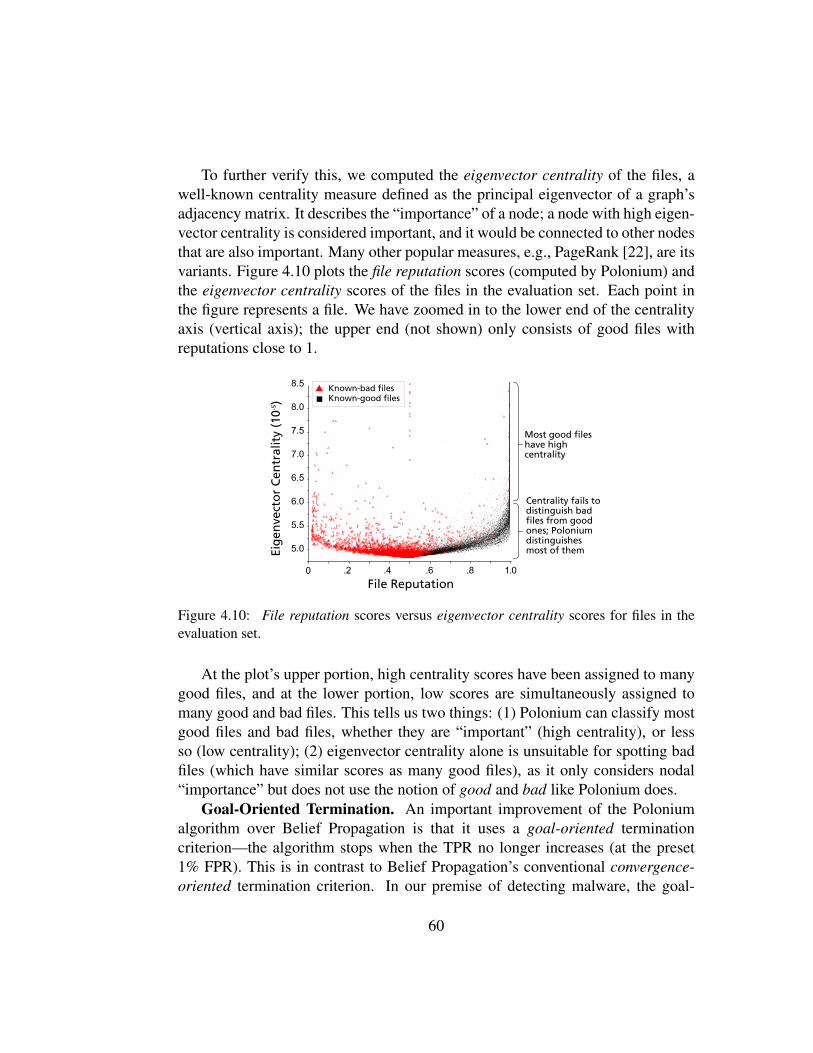
To further verify this, we computed the eigenvector centrality of the files, awell-known centrality measure defined as the principal eigenvector of a graph’sadjacency matrix. It describes the “importance” of a node; a node with high eigen-vector centrality is considered important, and it would be connected to other nodesthat are also important. Many other popular measures, e.g., PageRank [22], are itsvariants. Figure 4.10 plots the file reputation scores (computed by Polonium) andthe eigenvector centrality scores of the files in the evaluation set. Each point inthe figure represents a file. We have zoomed in to the lower end of the centralityaxis (vertical axis); the upper end (not shown) only consists of good files withreputations close to 1.

Figure 4.10: File reputation scores versus eigenvector centrality scores for files in theevaluation set.

At the plot’s upper portion, high centrality scores have been assigned to manygood files, and at the lower portion, low scores are simultaneously assigned tomany good and bad files. This tells us two things: (1) Polonium can classify mostgood files and bad files, whether they are “important” (high centrality), or lessso (low centrality); (2) eigenvector centrality alone is unsuitable for spotting badfiles (which have similar scores as many good files), as it only considers nodal“importance” but does not use the notion of good and bad like Polonium does.

Goal-Oriented Termination. An important improvement of the Poloniumalgorithm over Belief Propagation is that it uses a goal-oriented terminationcriterion—the algorithm stops when the TPR no longer increases (at the preset1% FPR). This is in contrast to Belief Propagation’s conventional convergence-oriented termination criterion. In our premise of detecting malware, the goal-

60

oriented approach is more desirable, because our goal is to classify software intogood or bad, at as high of a TPR as possible while maintaining low FPR — theconvergence-oriented approach does not promise this; in fact, node beliefs canconverge, but to undesirable values that incur poor classification accuracy. Wenote that in each iteration, we are trading FPR for TPR. That is, boosting TPRcomes with a cost of slightly increasing FPR. When the FPR is higher than desir-able, the algorithm stops.

4.5.3 ScalabilityWe ran the Polonium algorithm on the complete bipartite graph with 37 billionedges. Each iteration took about 3 hours to complete on average (∼185min). Thealgorithm scales linearly with the number of edges in the graph (O(|E|)), thanksto its adaptation of the Belief Propagation algorithm. We empirically evaluatedthis by running the algorithm on the full graph of over 37 billion edges, and on itssmaller billion-edge subgraphs with around 20B, 11.5B, 4.4B and 0.7B edges. Weplotted the per-iteration running times for these subgraphs in Figure 4.11, whichshows that the running time empirically achieved linear scale-up.

Figure 4.11: Scalability of Polonium. Running time per iteration is linear in the numberof edges.

4.5.4 Design and OptimizationsWe implemented two optimizations that dramatically reduce both running timeand storage requirement.

61

The first optimization eliminates the need to store the edge file in memory,which describes the graph structure, by externalizing it to disk. The edge filealone is over 200GB. We were able to do this only because the Polonium algo-rithm did not require random access to the edges and their associated messages;sequential access was sufficient. This same strategy may not apply readily to otheralgorithms.

The second optimization exploits the fact that the graph is bipartite (of ma-chines and files) to reduce both the storage and computation for messages byhalf [47]. We briefly explains this optimization here. LetBM [i, j](t) be the matrixof beliefs (for machine i and state j), at time t, and similarly BF [i, j](t) for thematrix of beliefs for the files. Because the graph is bipartite, we have

BM [i, j](t) = BF [i′, j′](t− 1) (4.3)BF [i′, j′](t) = BM [i, j](t− 1) (4.4)

In short, the two equations are completely decoupled, as indicated by the orangeand blue edges in Figure 4.12. Either stream of computations will arrive at thesame results, so we can choose to use either one (say following the orange arrows),eventually saving half of the effort.

Figure 4.12: Illustration of our optimization for the Polonium algorithm: since we havea bipartite graph (of files and machines), the naive version leads to two independent butequivalent paths of propagation of messages (orange, and blue arrows). Eliminating onepath saves us half of the computation and storage for messages, with no loss of accuracy.

4.6 Significance and ImpactIn August 2010, the Polonium technology was deployed, joining Symantec’s othermalware detection technologies to protect computer users from malware. Polo-nium now serves 120 million people around the globe (at the end of September2010). It has helped answer more than one trillion queries for file reputation.

62

Polonium’s effectiveness in the field has been empirically measured by se-curity experts at Symantec. They sampled live streams of files encountered bycomputer users, manually analyzed and labeled the files, then compared their ex-pert verdicts with those given by Polonium. They concluded that Polonium sig-nificantly lifted the detection rate of a collection of existing proprietary methodsby 10 absolute percentage points (while maintaining a false positive rate of 1%).This in-the-field evaluation is different from that performed over ground-truth data(described in Section 4.5), in that the files sampled (in the field) better exemplifythe types of malware that computer users around the globe are currently exposedto.

Our work provided concrete evidence that Polonium works well in practice,and it has the following significance for the software security domain:

1. It radically transforms the important problem of malware detection, typi-cally tackled with conventional signature-based methods, into a large-scaleinference problem.

2. It exemplifies that graph mining and inference algorithms, such as our adap-tation of Belief Propagation, can effectively unearth malware.

3. It demonstrates that our method’s detection effectiveness can be carried overfrom large-scale “lab study” to real tests “in the wild”.

4.7 Discussion

Handling the Influx of Data. The amount of raw data that Polonium works withhas almost doubled over the course of about 8 months, now exceeding 110 ter-abytes. Fortunately, Polonium’s time- and space-complexity both scale linearlyin the number of edges. However, we may be able to further reduce these re-quirements by applying existing research. Gonzalez et. al [52] have developeda parallelized version of Belief Propagation that runs on a multi-core, shared-memory framework, which unfortunately precludes us from readily applying it onour problem, as our current graph does not fit in memory.

Another possibility is to concurrently run multiple instances of our algorithm,one on each component of our graph. To test this method, we implemented asingle-machine version of the connected component algorithm [75] to find thecomponents in our graph, whose distribution (size versus count) is shown in Fig-ure 4.13; it follows the Power Law, echoing findings from previous research thatstudied million- and billion-node graphs [75, 97]. We see one giant component of

63

Figure 4.13: Component distribution of our file-machine bipartite graph, in log-log scale.

almost 950 million nodes (highlighted in red), which accounts for 99.77% of thenodes in our graph. This means our prospective strategy of running the algorithmon separate components will only save us very little time, if any at all! It is, how-ever, not too surprising that such a giant component exists, because most Windowscomputers uses similar subset of system files, and there are many popular appli-cations that many of our users may use (e.g., web browsers). These high-degreefiles connect machines to form the dominant component.

Recent research in using multi-machine architectures (e.g., Apache Hadoop)as a scalable data mining and machine learning platform [75, 70] could be a viablesolution to our rapidly increasing data size; the very recent work by Kang et.al [70] that introduced the Hadoop version of Belief Propagation is especiallyapplicable.

Perhaps, the simplest way to obtain the most substantial saving in computa-tion time would be to simply run the algorithm for one iteration, as hinted by thediminishing return phenomenon observed in out multi-iteration results (in Sec-tion 4.5). This deliberate departure from running the algorithm until convergenceinspires the optimization method that we discuss below.Incremental Update of File & Machine Reputation. Ideally, Polonium willneed to efficiently handle the arrival of new files and new machines, and it shouldbe able to determine any file’s reputation, whenever it is queried. The main ideais to approximate the file reputation, for fast query-time response, and replace theapproximation with a more accurate value after a full run of the algorithm. Ma-chine reputations can be updated in a similar fashion. The approximation dependson the maturity of a file. Here is one possibility:

Germinating. For a new file never seen before, or one that has only been re-

64

ported by very few machines (e.g., fewer than 5), the Polonium algorithmwould flag its reputation as “unknown” since there is too little information.

Maturing. As more machines report the file, Polonium starts to approximatethe file’s reputation through aggregating the reporting machines’ reputa-tions with one iteration of machine-to-file propagation; the approximationbecomes increasingly accurate over time, and eventually stabilizes.

Ripening. When a file’s reputation is close to stabilization, which can be deter-mined statistically or heuristically, Polonium can “freeze” this reputation,and avoid recomputing it, even if new reports arrive. Future queries aboutthat file will simply require looking up its reputation.

The NetProbe system [114], which uses Belief Propagation to spot fraudstersand accomplices on auction websites, used a similar method to perform incre-mental updates — the major difference is that we use a smaller induced subgraphconsisting of a file and its direct neighbors (machines), instead of the 3-hop neigh-borhood used by NetProbe, which will include most of the nodes in our highlyconnected graph.

4.8 ConclusionsWe motivated the need for alternative approaches to the classic problem of mal-ware detection. We transformed it into a large-scale graph mining and inferenceproblem, and we proposed the fast and scalable Polonium algorithm to solve it.Our goals were to infer the reputations of any files that computer users may en-counter, and identify the ones with poor reputation (i.e., malware).

We performed a large-scale evaluation of our method over a real machine-filegraph with one billion nodes and 37 billion edges constructed from the largestanonymized file submissions dataset ever published, spanning over 60 terabytesof disk space. The results showed that Polonium attained a high true positive rateof 87.1% TPR, at 1% FPR. We also verified Polonium’s effectiveness in the field;it has substantially lifted the detection rate of a collection of existing proprietarymethods by 10 absolute percentage points.

We detailed important design and implementation features of our method, andwe also discussed methods that could further speed up the algorithm and enable itto incrementally compute reputation for new files.

Our work makes significant contributions to the software security domain asit demonstrates that the classic malware detection problem may be approached

65

vastly differently, and could potentially be solved more effectively and efficiently;we offer Polonium as a promising solution. We are brining great impact to com-puter users around the world, better protecting them from the harm of malware.Polonium is now serving 120 million people, at the time of writing. It has helpedanswer more than one trillion queries for file reputation.

66

Part II

Mixed-Initiative GraphSensemaking

67

Overview

Even if Attention Routing (Part I) can provide good starting points for analysis, it isstill not enough. Much work in analytics is to understand why certain phenomenahappen (e.g., why those starting points are recommended?).

This task inherently involves a lot of exploration and hypothesis formulation,which we argue should best be carried out by integrating human’s intuition andexceptional perception skills with machine’s computation power. In this part, wedescribe mixed-initiative tools that achieve such human-in-the-loop graph mining,to help people explore and make sense of large graphs.• Apolo (Chapter 5), a mixed-initiative system that combines machine infer-

ence and visualization to guide the user to interactively explore large graphs.• Graphite (Chapter 6), a system that finds both exact and approximate

matches for graph patterns drawn by the user.

68

Chapter 5

Apolo: Machine Learning +Visualization for Graph Exploration

In Part I of this thesis, we described Attention Routing and its examples for findinggood starting points for analysis. But where should we go next, given those start-ing points? Which other nodes and edges of the graph should we explore next?This chapter describes Apolo, a system that uses a mixed-initiative approach—combining visualization, rich user interaction and machine learning—to guide theuser to incrementally and interactively explore large network data and make senseof it. In other words, Apolo could work with Attention Routing techniques to helpthe user expand from those recommended starting points.

Apolo engages the user in bottom-up sensemaking to gradually build up an un-derstanding over time by starting small, rather than starting big and drilling down.Apolo also helps users find relevant information by specifying exemplars, andthen using the Belief Propagation machine learning method to infer which othernodes may be of interest. We evaluated Apolo with 12 participants in a between-subjects study, with the task being to find relevant new papers to update an existingsurvey paper. Using expert judges, participants using Apolo found significantlymore relevant papers. Subjective feedback of Apolo was very positive.

Chapter adapted from work appeared at CHI 2011 [27]

69

Figure 5.1: Apolo displaying citation data around The Cost Structure of Sensemaking.The user has created three groups: Info Vis (blue) , Collaborative Search (orange), andPersonal Info Management (green). Colors are automatically assigned; saturation denotesrelevance. Dots appears under exampler nodes. 1: Config Panel for setting visibility ofedges, nodes and titles. 2: Filter Panel controls which types of nodes to show. 3: GroupPanel for creating groups. 4: Visualization Panel for exploring and visualizing network.Yellow halos surround articles whose titles contain “visual”.

5.1 Introduction

Making sense of large networks is an increasingly important problem in domainsranging from citation networks of scientific literature; social networks of friendsand colleagues; links between web pages in the World Wide Web; and personalinformation networks of emails, contacts, and appointments. Theories of sense-making provide a way to characterize and address the challenges faced by peopletrying to organize and understand large amounts of network-based data. Sense-making refers to the iterative process of building up a representation or schema ofan information space that is useful for achieving the user’s goal [128]. For exam-ple, a scientist interested in connecting her work to a new domain must build upa mental representation of the existing literature in the new domain to understandand contribute to it.

For the above scientist, she may forage to find papers that she thinks are rel-evant, and build up a representation of how those papers relate to each other. As

70

she continues to read more papers and realizes her mental model may not wellfit the data she may engage in representational shifts to alter her mental model tobetter match the data [128]. Such representational shifts is a hallmark of insightand problem solving, in which re-representing a problem in a different form canlead to previously unseen connections and solutions [63]. The practical impor-tance of organizing and re-representing information in the sensemaking processof knowledge workers has significant empirical and theoretical support [122].

We focus on helping people develop and evolve externalized representationsof their internal mental models to support sensemaking in large network data.Finding, filtering, and extracting information have already been the subjects ofsignificant research, involving both specific applications [38] and a rich varietyof general-purpose tools, including search engines, recommendation systems, andsummarization and extraction algorithms. However, just finding and filtering oreven reading items is not sufficient. Much of the heavy lifting in sensemaking isdone as people create, modify, and evaluate schemas of relations between items.Few tools aimed at helping users evolve representations and schemas. We build oninitial work such as Sensemaker [16] and studies by Russell et al. [127] aimed atsupporting the representation process. We view this as an opportunity to supportflexible, ad-hoc sensemaking through intelligent interfaces and algorithms.

These challenges in making sense of large network data motivated us to createApolo, a system that uses a mixed-initiative approach—combining rich user inter-action and machine learning—to guide the user to incrementally and interactivelyexplore large network data and make sense of it.

5.1.1 Contributions

Apolo intersects multiple research areas, naming graph mining, machine infer-ence, visualization and sensemaking. We refer our readers to the large amount ofrelevant work we surveyed in (Chapter 2).

However, less work explores how to better support graph sensemaking, likethe way Apolo does, by combining powerful methods from machine learning,visualization, and interaction.

Our main contributions are• We aptly select, adapt, and integrate work in machine learning and graph

visualization in a novel way to help users make sense of large graphs usinga mixed-initiative approach. Apolo goes beyond just graph exploration, andenables users to externalize, construct, and evolve their mental models of

71

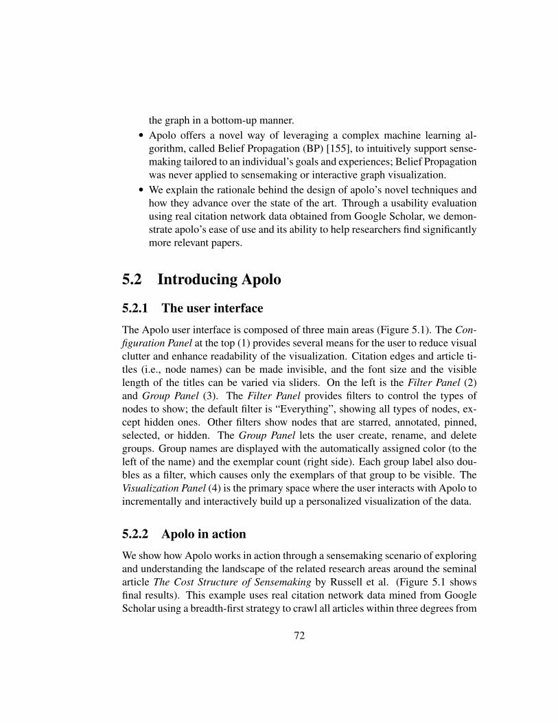
the graph in a bottom-up manner.• Apolo offers a novel way of leveraging a complex machine learning al-

gorithm, called Belief Propagation (BP) [155], to intuitively support sense-making tailored to an individual’s goals and experiences; Belief Propagationwas never applied to sensemaking or interactive graph visualization.

• We explain the rationale behind the design of apolo’s novel techniques andhow they advance over the state of the art. Through a usability evaluationusing real citation network data obtained from Google Scholar, we demon-strate apolo’s ease of use and its ability to help researchers find significantlymore relevant papers.

5.2 Introducing Apolo

5.2.1 The user interfaceThe Apolo user interface is composed of three main areas (Figure 5.1). The Con-figuration Panel at the top (1) provides several means for the user to reduce visualclutter and enhance readability of the visualization. Citation edges and article ti-tles (i.e., node names) can be made invisible, and the font size and the visiblelength of the titles can be varied via sliders. On the left is the Filter Panel (2)and Group Panel (3). The Filter Panel provides filters to control the types ofnodes to show; the default filter is “Everything”, showing all types of nodes, ex-cept hidden ones. Other filters show nodes that are starred, annotated, pinned,selected, or hidden. The Group Panel lets the user create, rename, and deletegroups. Group names are displayed with the automatically assigned color (to theleft of the name) and the exemplar count (right side). Each group label also dou-bles as a filter, which causes only the exemplars of that group to be visible. TheVisualization Panel (4) is the primary space where the user interacts with Apolo toincrementally and interactively build up a personalized visualization of the data.

5.2.2 Apolo in actionWe show how Apolo works in action through a sensemaking scenario of exploringand understanding the landscape of the related research areas around the seminalarticle The Cost Structure of Sensemaking by Russell et al. (Figure 5.1 showsfinal results). This example uses real citation network data mined from GoogleScholar using a breadth-first strategy to crawl all articles within three degrees from

72

the above paper. The dataset contains about 83,000 articles (nodes) and 150,000citations relationships (edges, each represents either a “citing” or “cited-by” re-lationships). This scenario will touch upon the interactions and major featuresof Apolo, and highlight how they work together to support sensemaking of largenetwork data. We will describe the features in greater depth in the next section.

We begin with a single source article highlighted in black in the center of theinterface (Figure 5.2a) and the ten most relevant articles as determined by thebuilt-in BP algorithm. Articles are shown as circles with sizes proportional totheir citation count. Citation relationships are represented by directed edges.

Figure 5.2: a) The Apolo user interface at start up, showing our starting article The CostStructure of Sensemaking highlighted in black. Its top 10 most relevant articles, havingthe highest proximity relative to our article, are also shown (in gray). We have selected ourpaper; its incident edges representing either “citing” (pointing away from it) or “cited-by”(pointing at it) relationships are in dark gray. All other edges are in light gray, to maximizecontrast and reduce visual clutter. Node size is proportional to an article’s citation count.Our user has created two groups: Collab Search and InfoVis (magnified). b-d) Our userfirst spatially separates the two groups of articles, Collab Search on the left and InfoVis onthe right (which also pins the nodes, indicated by white dots at center), then assigns themto the groups, making them exemplars and causing Apolo to compute the relevance of allother nodes, which is indicated by color saturation; the more saturated the color, the morelikely it belongs to the group. The image sequence shows how the node color changes asmore exemplars are added.

After viewing details of an article by mousing over it (Figure 5.3), the usermoves it to a place on the landscape he thinks appropriate, where it remains pinned

73

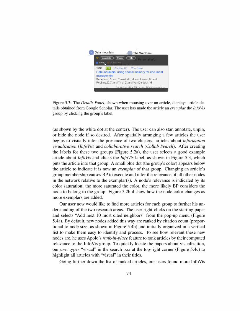
Figure 5.3: The Details Panel, shown when mousing over an article, displays article de-tails obtained from Google Scholar. The user has made the article an exemplar the InfoVisgroup by clicking the group’s label.

(as shown by the white dot at the center). The user can also star, annotate, unpin,or hide the node if so desired. After spatially arranging a few articles the userbegins to visually infer the presence of two clusters: articles about informationvisualization (InfoVis) and collaborative search (Collab Search). After creatingthe labels for these two groups (Figure 5.2a), the user selects a good examplearticle about InfoVis and clicks the InfoVis label, as shown in Figure 5.3, whichputs the article into that group. A small blue dot (the group’s color) appears belowthe article to indicate it is now an exemplar of that group. Changing an article’sgroup membership causes BP to execute and infer the relevance of all other nodesin the network relative to the exemplar(s). A node’s relevance is indicated by itscolor saturation; the more saturated the color, the more likely BP considers thenode to belong to the group. Figure 5.2b-d show how the node color changes asmore exemplars are added.

Our user now would like to find more articles for each group to further his un-derstanding of the two research areas. The user right-clicks on the starting paperand selects “Add next 10 most cited neighbors” from the pop-up menu (Figure5.4a). By default, new nodes added this way are ranked by citation count (propor-tional to node size, as shown in Figure 5.4b) and initially organized in a verticallist to make them easy to identify and process. To see how relevant these newnodes are, he uses Apolo’s rank-in-place feature to rank articles by their computedrelevance to the InfoVis group. To quickly locate the papers about visualization,our user types “visual” in the search box at the top-right corner (Figure 5.4c) tohighlight all articles with “visual” in their titles.

Going further down the list of ranked articles, our users found more InfoVis

74

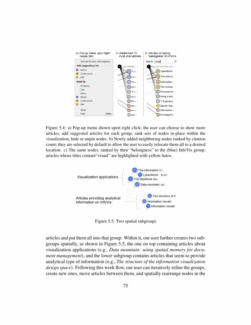
Figure 5.4: a) Pop-up menu shown upon right click; the user can choose to show morearticles, add suggested articles for each group, rank sets of nodes in-place within thevisualization, hide or unpin nodes. b) Newly added neighboring nodes ranked by citationcount; they are selected by default to allow the user to easily relocate them all to a desiredlocation. c) The same nodes, ranked by their “belongness” to the (blue) InfoVis group;articles whose titles contain“visual” are highlighted with yellow halos.

Figure 5.5: Two spatial subgroups

articles and put them all into that group. Within it, our user further creates two sub-groups spatially, as shown in Figure 5.5, the one on top containing articles aboutvisualization applications (e.g., Data mountain: using spatial memory for docu-ment management), and the lower subgroup contains articles that seem to provideanalytical type of information (e.g., The structure of the information visualizationdesign space). Following this work flow, our user can iteratively refine the groups,create new ones, move articles between them, and spatially rearrange nodes in the

75

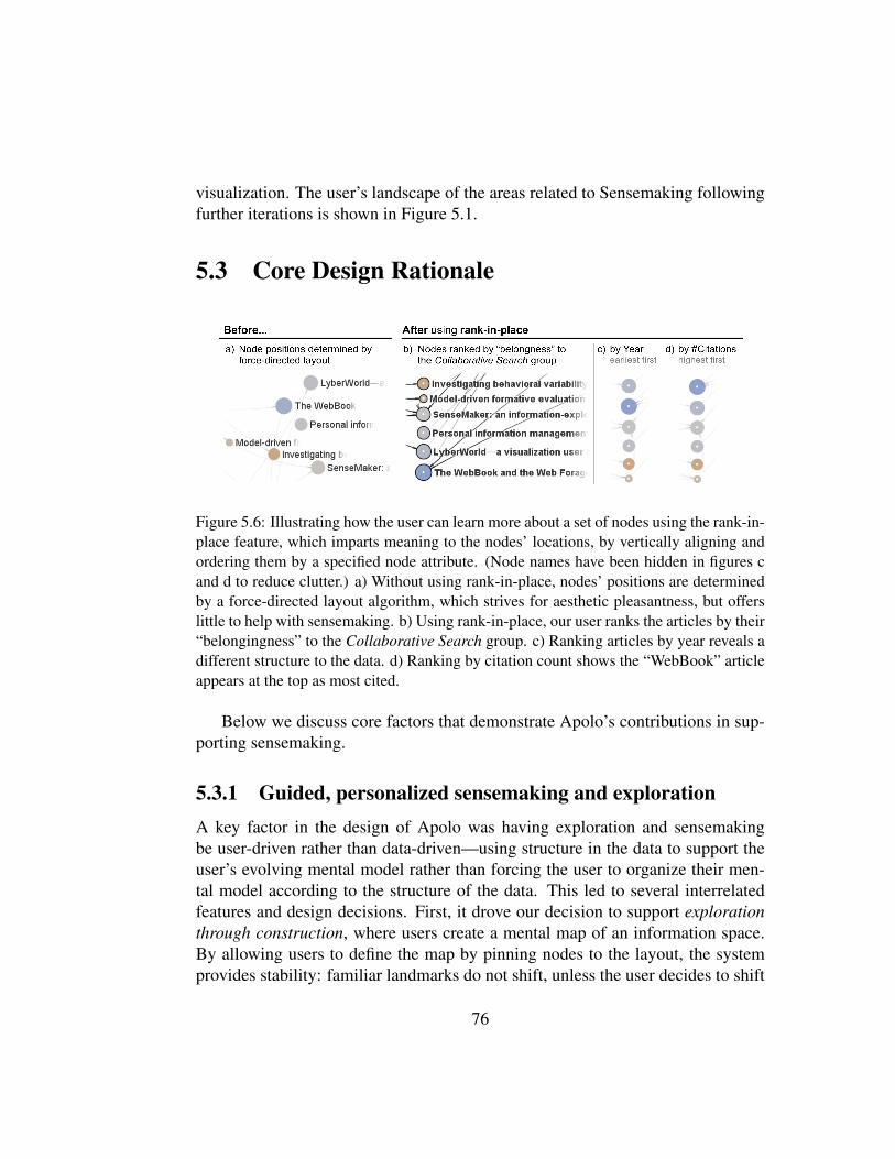
visualization. The user’s landscape of the areas related to Sensemaking followingfurther iterations is shown in Figure 5.1.

5.3 Core Design Rationale

Figure 5.6: Illustrating how the user can learn more about a set of nodes using the rank-in-place feature, which imparts meaning to the nodes’ locations, by vertically aligning andordering them by a specified node attribute. (Node names have been hidden in figures cand d to reduce clutter.) a) Without using rank-in-place, nodes’ positions are determinedby a force-directed layout algorithm, which strives for aesthetic pleasantness, but offerslittle to help with sensemaking. b) Using rank-in-place, our user ranks the articles by their“belongingness” to the Collaborative Search group. c) Ranking articles by year reveals adifferent structure to the data. d) Ranking by citation count shows the “WebBook” articleappears at the top as most cited.

Below we discuss core factors that demonstrate Apolo’s contributions in sup-porting sensemaking.

5.3.1 Guided, personalized sensemaking and explorationA key factor in the design of Apolo was having exploration and sensemakingbe user-driven rather than data-driven—using structure in the data to support theuser’s evolving mental model rather than forcing the user to organize their men-tal model according to the structure of the data. This led to several interrelatedfeatures and design decisions. First, it drove our decision to support explorationthrough construction, where users create a mental map of an information space.By allowing users to define the map by pinning nodes to the layout, the systemprovides stability: familiar landmarks do not shift, unless the user decides to shift

76

them. Contrast this to a pure force-directed layout algorithm, which may placeitems in a different location every time or shift all items when one is moved.apolo’s support for hybrid layout, mixing user-driven and automatic layout, is alsodifferent from work on semi-automatic layout (e.g., [129]) that uses constraints toimprove a final layout, whereas Apolo supports constraints (fixing node positions)to help users evolve and externalize their mental models.

Second, instead of using an unsupervised graph clustering algorithm thatuses the same similarity space for every user (as in [120]), we adapted a semi-supervised algorithm (Belief Propagation) that would fundamentally change thestructure of the similarity space based on user-labeled exemplars. Apolo uses thisalgorithm to find relevant nodes when starting up or when the user asks for group-or paper-relevant nodes, and to quantify relevance for use in ranking-in-place orindicating relevance through color. This means that even if two users’ landscapesincluded the same nodes, those landscapes could be very different based on theirgoals and prior experience.

5.3.2 Multi-group Sensemaking of Network DataAnother important factor was the ability to support multiple dynamic, example-based groups. Theories of categorization suggest that people represent categoriesand schemas through examples or prototypes [126], as opposed to what are typicalway of interacting with collections of information online such as search queriesor tags. Furthermore, items may and often do belong to multiple groups, leadingto a need for “soft” clustering.

Apolo was designed to support multiple groups both in the interface and al-gorithmically. In the interface, users can easily create multiple groups and movenodes into and out of one or more groups (via the Details Panel, Figure 5.3).Users can also see the degree to which the algorithm predicts items to be in agroup through color. The use of the BP algorithm is instrumental as it can sup-port fast, soft clustering on an arbitrary number of groups; many graph-basedspreading activation-style algorithms are limited to one or two groups (such asPageRank [22], and random walk with restart [144]).

5.3.3 Evaluating exploration and sensemaking progressSensemaking involves evolution and re-representation of the user’s mental model.Users typically continue evolving their models until they stop encountering newinformation; when the new information they encounter confirms rather than

77

changes their existing mental representations; and when their representations aresufficiently developed to meet their goals. To assist in this evaluation process,Apolo surfaces change-relevant information in a number of ways. It helps theuser keep track of which items have been seen or hidden. New nodes are addedin a systematic way (Figure 5.4), to avoid disorienting the user. Pinned nodesserve as fixed landmarks in the users’ mental map of the information space andcan only be moved through direct action by the user. When saving and loading theinformation space, all pinned nodes remain where the user put them. Apolo usesall these features together to preserve the mental map that the user has developedabout the graph structure over time [104].

As a node’s group membership can be “toggled” easily, the user can experi-ment with moving a node in and out of a group to see how the relevance of theother nodes change, as visualized through the nodes’ color changes; thus the ef-fect of adding more exemplars (or removing them) is easily apparent. Also, colorchanges diminishing over time can help indicate the user’s representations stabi-lizing.

Figure 5.7: Our user applies two rank-in-place arrangements to the exemplars of Collabo-rative Search group (left, ranked by their “belongness” to the group) and the InfoVis group(right, ranked by year). These two side-by-side arrangements reveal several insights: 1)the Collaborative Search articles are less cited (smaller node sizes), as the research ismore recent; 2) only the article Exploratory Search in the Collaborative Search groupcited the source paper, while three papers in the InfoVis has either cited or been cited bythe source paper.

78

5.3.4 Rank-in-place: adding meaning to node placementTypically, layout algorithms for graphs (e.g., force-based layouts) try to layoutnodes to minimize occlusion of nodes and edges, or to attain certain aestheticrequirements [41]. These layouts usually offer little help with the sensemakingprocess. Approaches to address this problem include “linked views”, which use aseparate view of the data (e.g., scatter plot) to aid node comparison; and impartingmeaning to the node locations (e.g., in NodeXL [134] and PivotGraph [149]).However, the above approaches are often global in nature: all nodes in the networkare repositioned, or a new, dedicated visualization created.

Apolo’s main difference is that it offers a rank-in-place feature that can ranklocal subsets of nodes in meaningful ways. Figure 5.6 shows one such example.Furthermore, the user can create multiple, simultaneous arrangements (throughranking) for different sets of nodes, which can have independent arrangementcriteria (e.g., one ranks by year, the other ranks by citation count). We designedfor this flexibility to allow other characteristics of the nodes (e.g., their edges,node sizes) to still be readily available, which may then be used in tandem with thenode arrangement across multiple rankings (see Figure 5.7). Recently, researchersare exploring techniques similar to rank-in-place, to create scatterplots within anetwork visualization [147].

5.4 Implementation & Development

5.4.1 Informed design through iterationsSensemaking for large network data is an important problem which will undoubt-edly take years of research to address. As such, our Apolo system only solves partof it; however, the system’s current design is the result of over two years’ investi-gation and development effort through many iterations and two major revisions.

The first version of Apolo presented suggestions in ranked lists without a vi-sualization component (Figure 5.8), one list for each group in a floating window.Users’ exemplars showed up at the top of the lists with the most relevant itemsin ranked order below them . We initially thought that the high data density andease of comprehension of the list format might lead to better performance than aspatial layout. However, our users quickly pointed out the lack of a spatial layout,both as a workspace to externalize their mental representations as well as to under-stand the relations between items and between groups. This finding prompted usto add a network visualization component to the second revision. While working

79

towards the second revision, we conducted contextual inquiries with six graduatestudents to better understand how they make sense of unfamiliar research topicsthrough literature searches. We learned that they often started with some familiararticles, then tried to find works relevant to them, typically first considering thearticles that cited or were cited by their familiar articles. Next, they consideredthose new articles’ citation lists. And they would repeat this process until theyhad found enough relevant articles. This finding prompted us to add support forincremental, link-based exploration of the graph data.

Figure 5.8: The first version of Apolo

We studied the usability of the second revision through a pilot study, where welet a few researchers use Apolo to make sense of the literature around new topicsthat they recently came across. We learned that (1) they had a strong preference inusing spatial arrangement to manage their exploration context, and to temporarilyorganize articles into approximate (spatial) groups; (2) they used the visualiza-tion directly most of the time, to see relations between articles and groups, andthey only used the list for ranking articles. These findings prompted us to rethinkapolo’s interaction design, and inspired us to come up with the rank-in-place tech-nique that offers benefits of both a list-based approach and a spatial layout. Rank-in-place lays out nodes at a greater density, while keeping them quick to read andtheir relations easy to trace. With this new technique, we no longer needed thesuggestion lists, and the visualization became the primary workspace in apolo.

80

5.4.2 System Implementation

The Apolo system is written in Java 1.6. It uses the JUNG library [112] for visu-alizing the network. The network data is stored in an SQLite embedded database(www.sqlite.org), for its cross-platform portability and scalability up to tens ofgigabytes. One of our goals is to offer Apolo as a sensemaking tool that work ona wide range of network data, so we designed the network database schema inde-pendently from the Apolo system, so that Apolo can readily be used on differentnetwork datasets that follow the schema.

We implemented Belief Propagation as described in [98]. The key settings ofthe algorithm include: (1) a node potential function that represents how likely anode belongs to each group (a value closer to 1 means more likely), e.g., if wehave two groups, then we assign (0.99, 0.01) to exemplars of group 1, and (0.5,0.5) to all other nodes; (2) an edge potential function that governs to what extentan exemplar would convert its neighbors into the same group as the exemplar (avalue of 1 means immediate conversion; we used 0.58).

5.5 EvaluationTo evaluate Apolo, we conducted a laboratory study to assess how well peoplecould use Apolo on a sensemaking task on citation data of scientific literature. Ata high-level, we asked participants to find papers that could be used to update therelated work section of a highly cited survey paper describing software tools forHCI [105]. We considered using other datasets such as movie data, but we feltthat evaluation could be too subjective (genres are hard to define). In contrast, sci-entific literature provides a good balance between objectivity (some well-knownresearch areas) and subjectivity (subject’s different research experience). Anotherreason we chose scientific literature was because it was easier to assess “ground-truth” for evaluating the study results. More specifically, we used literature fromcomputer science research areas of HCI (i.e., UIST), and had experts at our insti-tution help establish “ground truth.”

5.5.1 Participants

We recruited twelve participants from our university through a recruitment website managed by our institution and through advertisements posted to a universitymessage board. All participants were either research staff or students, and all had

81

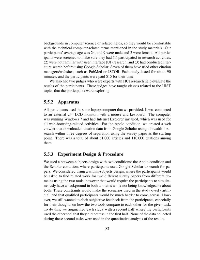
backgrounds in computer science or related fields, so they would be comfortablewith the technical computer-related terms mentioned in the study materials. Ourparticipants’ average age was 24, and 9 were male and 3 were female. All partic-ipants were screened to make sure they had (1) participated in research activities,(2) were not familiar with user interface (UI) research, and (3) had conducted liter-ature search before using Google Scholar. Seven of them have used other citationmanagers/websites, such as PubMed or JSTOR. Each study lasted for about 90minutes, and the participants were paid $15 for their time.

We also had two judges who were experts with HCI research help evaluate theresults of the participants. These judges have taught classes related to the UISTtopics that the participants were exploring.

5.5.2 ApparatusAll participants used the same laptop computer that we provided. It was connectedto an external 24” LCD monitor, with a mouse and keyboard. The computerwas running Windows 7 and had Internet Explorer installed, which was used forall web-browsing-related activities. For the Apolo condition, we created a webcrawler that downloaded citation data from Google Scholar using a breadth-first-search within three degrees of separation using the survey paper as the startingpoint. There was a total of about 61,000 articles and 110,000 citations amongthem.

5.5.3 Experiment Design & ProcedureWe used a between-subjects design with two conditions: the Apolo condition andthe Scholar condition, where participants used Google Scholar to search for pa-pers. We considered using a within-subjects design, where the participants wouldbe asked to find related work for two different survey papers from different do-mains using the two tools; however that would require the participants to simulta-neously have a background in both domains while not being knowledgeable aboutboth. These constraints would make the scenarios used in the study overly artifi-cial, and that qualified participants would be much harder to come across. How-ever, we still wanted to elicit subjective feedback from the participants, especiallyfor their thoughts on how the two tools compare to each other for the given task.To do this, we augmented each study with a second half where the participantsused the other tool that they did not use in the first half. None of the data collectedduring these second tasks were used in the quantitative analysis of the results.

82

We asked participants to imagine themselves as researchers new to researchin user interfaces (UI) who were tasked with updating an existing survey paperpublished in 2000. The participants were asked to find potentially relevant paperspublished since then, where relevant was defined as papers that they would want toinclude in an updated version. We felt that defining “relevant” was necessary andwould be understandable by researchers. Given that finding relevant papers for theentire survey paper would be a very extensive task, both for participants and forthe judges, we asked participants to focus on only two of the themes presented inthe survey paper: automatically generating user interfaces based on models andrapid prototyping tools for physical devices, not just software (both paraphrased),which were in fact section titles in the paper.

In each condition, the participants spent 25 minutes on the literature searchtask. They were to spend the first 20 minutes to collect relevant articles, thenthe remaining five to select, for each category, 10 that they thought were mostrelevant. They did not have to rank them. We limited the time to 25 minutes tosimulate a quick first pass filter on papers. In the Google Scholar condition, weset the “year filter” to the year 2000 so it would only return articles that werepublished on or after that year. In the Apolo condition, we started people with thesurvey paper. Participants in the Apolo condition were given an overview of thedifferent parts of Apolo’s user interface and interaction techniques, and a sheet ofpaper describing its main features.

5.5.4 ResultsWe examined our results using both a quantitative approach as well as subjectmeasures. We pooled together all the articles that the participants found in thestudy and divided them into two stacks, “model-based” and “prototyping”, ac-cording to how they were specified by the participants. For each article, we lo-cated a soft copy (usually a PDF) and printed out the paper title, abstract andauthor information. We collected these printouts and sorted them alphabetically.These printouts were used by the expert judges. We had the two judges selectpapers relevant to the topic. We represented each expert’s judgment as a vectorof 0s and 1s. An article was marked with “1” if the expert considered it relevant,and “0” otherwise. We used cosine similarity to evaluate the similarity betweenthe two experts. A score of 1 means complete agreement, and 0 means completedisagreement. For the “Model-based” articles, the cosine similarity between theexperts’ judgement was 0.97. For the “Prototyping” articles, despite few papersbeing considered relevant by the judges, the cosine similarity was 0.86.

83

Figure 5.9: a) Average combined judges’ scores; an article from a participant receives ascore of 1 when it is considered relevant by an expert (min is 0, max is 2). The averagescore across both categories was significantly higher in the Apolo condition. Error barsrepresent -1 stdev, * indicates statistically significant. b) The number of articles consid-ered relevant by the two expert judges (blue and orange). The total number of articlesfound by participants are in gray. The two experts strongly agree with each other in theirjudgment.

In our evaluation, the independent factor is “participant”, and the dependentfactor is the relevance scores assigned by the expert judges. Using a two-tailedt-test, we found the average score across both categories was significantly higherin the Apolo condition (t(9.7) = 2.32, p < 0.022), as shown in Figure 5.9a. Wealso note that participants in both conditions did well for finding papers related tomodel-based interfaces. One reason for this is that papers in this category tendedto have the word “automatic” or “model” in the title. However, the same was nottrue for papers in the prototyping category.

5.5.5 Subjective ResultsOverall, participants felt that Apolo improved their sensemaking experience.Based on a post-test survey, Apolo seemed to be easy to use, as shown in Figure5.10 and 5.11. These results are encouraging given that Apolo was not designedas a walk-up-and-use system.

We organized qualitative feedback from participants into three categories. Thefirst relates to general sensemaking and organization. One participant said thatApolo “helped much more in organizing search[...] Google was a bit random.”The graph visualization was also helpful. One person said that it “helped me seethe citation network in which articles cited which ones”. Another said that the “in-

84

Figure 5.10: Subjective ratings of Apolo. Participants rated Apolo favorably. Features forgrouping, suggesting and ranking nodes, were highly rated. Apolo’s usage was very clearto most participants (green bar).

dication of degree relevance by color was extremely helpful and easy to use and italso helped to make sense of the articles.” Being able to spatially organize paperswas also a useful feature and participants were happy about using it. One personsaid that “arrangement of articles in my order of preference & my preferred loca-tion was easy.” We do note that the task that we had participants do was somewhatlimited in scale, but for the current task the screen real estate available was suffi-cient. Seeing connections between papers was also helpful. Participants said that“it helped me see the citation network in which articles cited which ones”, andthat it was an “easy way to list & relate citations graphically.” Participants alsohad constructive feedback for improving Apolo. One comment was to have ab-stracts be more readily available in Apolo (a constraint of the crawling software,since Google Scholar does not have full abstracts in an accessible format). An-other comment was that there would often be too many edges, a problem commonto graph visualizations.

85

Figure 5.11: Participants liked and enjoyed using Apolo, and would like to use it again inthe future. They generally found Apolo more useful than Google Scholar in helping themfind relevant articles and make sense of them.

5.5.6 Limitations

While the results of our evaluation was positive, there are also several limitations.For example, we only had participants examine two themes. Having more themeswould stress the screen real estate. Apolo currently has minimal features for man-aging screen real estate.

We also did not evaluate category creation and removal; participants weregiven two categories that correspond to two sections in the given overview paper,which may not be the most natural categories that they would like to create. How-ever, if we were to allow the participants to create any group they wanted, the greatvariety of possible groups created would make our evaluation extremely difficult.Moreover, a pilot study found that more categories required more prior knowledgethan participants would have. Two categories were in fact already challenging, asindicated by the few relevant articles found for the “Prototyping” group.

The need for the participants to categorize articles was created by the tasks;however, in real-world scenarios, such needs would be ad hoc. We plan to studysuch needs, as well as how Apolo can handle those kinds of tasks, in less con-trolled situations. For example, how many groups do people create? Do thegroupings evolve over time, such as through merging or subdivision. How welldo the findings of sensemaking literature apply to large graph data?

5.6 Discussion

Mixed-initiative approaches for network exploration are becoming increasinglyimportant as more datasets with millions or even billions of nodes and edges are

86

becoming available. These numbers vastly exceed people’s limited cognitive ca-pacities. By combining a person’s reasoning skills with computer algorithms forprocessing large amounts of data, we hope to reduce the disparity in gaining accessto and comprehending the vast amount of graph data that have become increas-ingly available. Automated analysis methods and algorithms for extracting usefulinformation, such as patterns and anomalies, are active research topics. However,these methods can rarely give the perfect solutions, or even if they can, it is nec-essary to convey such information to the user. Our work seeks to reach the goalof supporting sensemaking through a mix of rich user interaction and machinelearning.

Visually managing many nodes is also an open problem in graph sensemaking;Apolo currently focuses on filtering, e.g. enabling users to remove nodes fromthe visualization, re-add them, or focus only on selected ones. By integratingBelief Propagation, we hope to help users find relevant nodes quickly and removeunnecessary nodes from the visualization more easily than a manual approach.We have been experimenting with methods that will help further, such as semanticzooming, and reversibly collapsing nodes into meta nodes.

Apolo currently relies exclusively on the link-structure of a graph to makerelevance judgments. In the future, we would like to integrate other types of infor-mation as well, such as the textual content of the nodes and edges (e.g., the contentof an article), edge weights, and temporal information (particularly important foranalyzing dynamic networks).

5.7 ConclusionsApolo is a mixed-initiative system for helping users make sense of large networkdata. It tightly couples large scale machine learning with rich interaction and visu-alization features to help people explore graphs through constructing personalizedinformation landscapes. We demonstrate the utility of Apolo through a scenarioand evaluation of sensemaking in scientific literature. The results of the evaluationsuggest the system provides significant benefits to sensemaking and was viewedpositively by users. This work focuses on the scientific literature domain; a recentwork [69] showed that approaches similar to ours (based on spreading activation)could also work well for graph data of websites and tags, supporting that the ideasin Apolo can be helpful for many other kinds of data intensive domains, by aid-ing analysts in sifting through large amounts of data and directing users’ focus tointeresting items.

87

88

Chapter 6

Graphite: Finding User-SpecifiedSubgraphs

The previous chapter describes the Apolo system that helps the user explore largegraphs by starting with some nodes of interest. Apolo assumes the user knowswhich specific nodes to start with. But what about when the user only has somerough idea about what they are looking for?

This chapter presents GRAPHITE, a system that enables the user to find bothexact and approximate matching subgraphs in large attributed graphs, based ononly fuzzy descriptions that the user draws graphically.

For example, in a social network where a person’s occupation is an attribute,the user can draw a ‘star’ query for “finding a CEO who has interacted with aSecretary, a Manager, and an Accountant, or a structure very similar to this”.GRAPHITE uses the G-Ray algorithm to run the query against a user-chosen datagraph, gaining all of its benefits, namely its high speed, scalability, and its abilityto find both exact and near matches. Therefore, for the example above, GRAPHITE

tolerates indirect paths between, say, the CEO and the Accountant, when no directpath exists. GRAPHITE uses fast algorithms to estimate node proximities whenfinding matches, enabling it to scale well with the graph database size.

We demonstrate GRAPHITE’s usage and benefits using the DBLP author-publication graph, which consists of 356K nodes and 1.9M edges. A demo videoof GRAPHITE can be downloaded at http://youtu.be/nZYHazugVNA.

Chapter adapted from work appeared at ICDM 2008 [30]

89

6.1 Introduction

Figure 6.1: The GRAPHITE user interface showing the query pattern (left) for a chainof authors from four different conferences. Nodes are authors; attributes are conferences;edges indicate co-authorship. One best-effort match (right) is Indyk (STOC), Muthu (SIG-MOD), Garofalakis bridging Muthu and Jordan (ICML), and Hinton bridging Jordan andFels (ISBMS).

People often want to find patterns in graphs, such as social networks, to bet-ter understand their dynamics. One such use is to spot anomalies. For example,in social networks where a person’s occupation is an attribute, we might want tofind money laundering rings that consist of alternating businessmen and bankers.But, then, we face several challenges: (1) we need a conveninent way to specifythis ring pattern as a query, with appropriate attributes (e.g., businessman, banker)assigned to each node; (2) we need to find all potential matches for this pattern;we want near matches as well, such as allowing another person between a busi-nessman and a banker, because we may not know the exact structure of a moneylaundering ring; (3) the graph matching process should be fast, avoiding expen-sive operations, such as joins; (4) we want to visualize all the matches to better

90

interpret them.We present GRAPHITE, a system designed to solve the above challenges.

GRAPHITE stands for Graph Investigation by Topological Example. It providesa usable integrated environment for handling the complete workflow of queryinga large graph for subgraph patterns. Users can (1) naturally draw the structure ofthe pattern they want to find and assign attribute values to nodes; (2) run the queryagainst a user-chosen data graph, using the G-Ray method, to quickly locate exactand near matches; (3) obtain matches in a matter of seconds; and (4) visualize thematches.

Figure 6.1 is a screenshot of GRAPHITE when we ask for a chain of four coau-thors in DBLP: a STOC’05 author, a SIGMOD’06 author, an ICML’93 author, andan ISBM’05 author. Such a chain does not exist, but GRAPHITE returns a best-effort match, with two intermediate nodes (in white): Minos Garofalakis, whobridges Muthu (SIGMOD) with Jordan (ICML, a premier machine learning con-ference) and Geoffrey Hinton, who bridges Michael Jordan (ICML) and SidneyFels (ISBMS, a conference on biomedical simulation).

This work is organized as follows. Section 6.2 gives the formal definition ofour subgraph matching problem. Section 6.3 describes the system details. Section6.4 describes what we will be demonstrating for GRAPHITE. Section 6.5 discussesrelated work. We conclude our contributions in Section 6.6.

6.2 Problem Definition

We describe the subgraph matching problem that GRAPHITE is designed to solve.Consider the fictitious social network in Figure 6.2, where nodes are people,whose attributes (job titles) are represented by shapes and colors. We define theproblem as:

Given

• a data graph (e.g., Figure 6.2), where the nodes have one categoricalattribute, such as job titles,

• a query subgraph describing the configuration of nodes that the userwants to find (e.g., Figure 6.3(a)), and

• the number of desired matching subgraphs k,

find k matching subgraphs, that match the query as well as possible.

91

Figure 6.2: A ficticious network of people, whose job titles (attributes) are represented byshapes and colors.

(a) Loop query (b) A matching subgraph

Figure 6.3: A loop query and a match

For inexact matches, they should be ranked accordingly to their quality, suchas how “similar” they look to the query. Incidentally, since we are using the G-Ray algorithm, the matching subgraphs will be automatically ranked according toits goodness function, giving convincing and intuitive rankings [143].

6.3 Introducing GraphiteGRAPHITE is a system for visually querying large social networks through directmanipulation, finding exact and near matches, and visualizing them.

The User Interface and Interactions. Figure 6.4 shows GRAPHITE’s userinterface. The left half is the query area (a), where users draw their query sub-graphs. They can assign an attribute to a node by double-clicking on it and picking

92

Figure 6.4: The GRAPHITE user interface. (a) User-specified ‘star’ query pattern. (b) Nearmatch for the ‘star’ pattern. Nodes are authors; attributes are conferences; edges link co-authors. The query asks for an author who has published in PODS, with connections toauthors of IAT, PODS, and ISBMS. (c) Users can select, create, move and delete nodesand edges; they can also zoom and pan. (d) Users specify number of matches. (e) Matchesshown as tabs. (f) Users double-click a node to bring up a dialog for filtering attributesdown to the ones that contain the filtering text.

a value from a pop-up dialog (f). Users can create nodes and edges with the edit-ing control (middle icon at (c)), reposition or delete them with the picking control(arrow icon at (c)), pan around the view port with the panning control (hand iconat (c)), and zoom in or out with the mouse scroll wheel. The right half of the userinterface is the results area (b), which shows the exact and near matches as tabs(e) that the user can inspect conveniently by flipping through them. Users canspecify the number of matches they want to find with the text box at the bottom ofthe interface (d). They can then click the Find Matches button to start the patternmatching process.

Algorithm for Finding Matches. There are many different subgraph match-ing algorithms that could be used for GRAPHITE; if we only wanted exactmatches, we could write SQL queries to specify the query patterns. However,we chose the G-Ray algorithm for the following two advantages. First, when noexact matches exist, it automatically searches for best-effort matches (tolerating

93

longer, indirect paths). Second, thanks to its proposed goodness function [143], itranks the resulting matches, returning results that are empirically more importantto the users, thus avoids flooding the user with a potentially huge number of lessimportant matches.

Implementation. GRAPHITE is a Java SE 6 application. It uses the JUNG1

Java library for editing and visualizing graphs. G-Ray, the backend algorithm thatGRAPHITE uses for subgraph matching is written in the MATLAB programminglanguage. GRAPHITE uses the RemoteMatLab software library2 to remotely callinto an instance of MATLAB that has been started as a server, passing querypatterns to the algorithm and obtaining matches from it.

6.4 Example ScenariosWe illustrate GRAPHITE’s usage through several example scenarios.

Datasets. We use the DBLP dataset,3 from which we construct an attributedgraph where each node is an author and the node’s attribute is the combinationof a conference name and a year (e.g., “ICDM 2008”). We describe this at-tributed graph by two matrices: (1) a node-to-node matrix, which represents theco-authorship among authors where entry (i, j) is the number of coauthored papersbetween author i and j; and (2) a node-to-attribute matrix, which represents theauthor-conference relationship where entry (i, j) equals 1 if author i has publishedin conference j, and 0 otherwise. In total, there are 356,364 nodes, 1,905,970edges, and 12,920 possible attribute values.

Scenarios. In Figure 6.4, the ‘star’ query asks for an author who has pub-lished in PODS (in red), who has co-authored papers with three other authorsfrom the conferences IAT (orange), PODS (red), and ISBMS (yellow). In oneof the highest-ranking matches (on the right), the PODS author in the center isPhilip Yu, a prolific author in databases and data mining. The other PODS authoris Hector Garcia-Molina, also extremely prolific, with an indirect connection toPhilip through Chawathe, his ex-advisee. Zhongfei (Mark) Zhang is the matchingauthor for IAT, Intelligent Agent Technology, who is a computer vision researcherwith a recent interest in data mining, hence the connection to Philip Yu. Similarly,Figure 6.1 shows a ‘line’ pattern.

1http://jung.sourceforge.net/2http://plasmapowered.com/wiki/index.php/Calling_MatLab_from_

Java3http://www.informatik.uni-trier.de/˜ley/db/

94

6.5 Related WorkGraph matching algorithms vary widely due to differences in the specific problemsthey address. G-Ray is a fast approximate algorithm for inexact pattern match-ing in large, attributed graphs. It extends the ideas of connection subgraphs [46]and centerpiece graphs [142] and applies them to pattern matching in attributedgraphs. This work is also related to the idea of network proximity, which buildson connection subgraphs [85].

Our work focuses on finding instances of user-specified patterns in graphs.Graph mining work in the database literature focuses on related problems, like thediscovery of frequent or interesting patterns [153], near-cliques [119], and inexactquerying of databases [20]. However, none of these methods can do ‘best-effort’matching for arbitrary shapes, like loops, that GRAPHITE can handle. For morediscussion and a survey of graph matching algorithms, please refer to Section 2.1.

6.6 ConclusionsWe present GRAPHITE, a system for visually querying large graphs. GRAPHITE’scontributions include (1) providing an integrated environment for handling thecomplete workflow of querying a large graph for subgraph patterns; (2) providingan intuitive means for users to specify query patterns by simply drawing them;(3) finding and ranking both exact and near matches, using the best-effort G-Rayalgorithm; (4) visualizing matches to assist users in understanding and interpret-ing the results; and (5) delivering results in high speed for large graphs (such asthe DBLP graph, consisting of 356K nodes), returning results in seconds, on acommodity PC.

GRAPHITE can become a useful tool for scientists and analysts working ongraph problems to quickly find patterns of their choosing, to experiment with andto confirm their speculations.

95

Part III

Scaling Up for Big Data

96

Overview

Massive graphs, having billions of nodes and edges, do not fit in the memory of asingle machine, and not even on a single hard disk. In this part, we describe toolsand methods to scale up computation for speed and with data size.• Parallelism with Hadoop (Chapter 7): we scale up the Belief Propagation

(BP) algorithm to billion-node graphs, by leveraging Hadoop. BP is a pow-erful inference algorithm successfully applied on many important problems,e.g., computer vision, error-correcting codes, fraud detection (Chapter 3).

• Approximate Computation (Chapter 8): we contribute theories and algo-rithms to further speed up Belief Propagation by two folds, and to improveits accuracy.

• Staging of Operations (Chapter 9): our OPAvion system adopts a hybridapproach that maximizes scalability for algorithms using Hadoop, whileenabling interactivity for visualization by using the user’s local computer asa cache.

97

Chapter 7

Belief Propagation on Hadoop

Belief Propagation (BP) is a powerful inference algorithm successfully appliedon many different problems; we have adapted it for our work in fraud detection(Chapter 3), malware detection (Chapter 4), and graph exploration (Chapter 5). Inthose works, we implemented the algorithm to run on a single machine, becausethose graphs fit on a single disk (even for Polonium’s 37 billion edge graph). Butgraphs are now bigger, and do not fit on one disk anymore. What to do then?

This chapter describes how to leverage the HADOOP platform to scale up in-ference through our proposed HADOOP LINE GRAPH FIXED POINT (HA-LFP),an efficient parallel algorithm for sparse billion-scale graphs.

Our contributions include (a) the design of HA-LFP, observing that it cor-responds to a fixed point on a line graph induced from the original graph; (b)scalability analysis, showing that our algorithm scales up well with the numberof edges, as well as with the number of machines; and (c) experimental resultson two private, as well as two of the largest publicly available graphs — the WebGraphs from Yahoo! (6.6 billion edges and 0.24 Tera bytes), and the Twitter graph(3.7 billion edges and 0.13 Tera bytes). We evaluated our algorithm using M45,one of the top 50 fastest supercomputers in the world, and we report patterns andanomalies discovered by our algorithm, which would be invisible otherwise.

Chapter adapted from work appeared at ICDE 2011 [71]

98

7.1 Introduction

Given a large graph, with millions or billions of nodes, how can we find patternsand anomalies? One method to do that is through “guilt by association”: if weknow that nodes of type “A” (say, males) tend to interact/date nodes of type “B”(females), we can infer the unknown gender of a node, by checking the genderof the majority of its contacts. Similarly, if a node is a telemarketer, most of itscontacts will be normal phone users (and not telemarketers, or 800 numbers).

We show that the “guilt by association” approach can find useful patterns andanomalies, in large, real graphs. The typical way to handle this is through theso-called Belief Propagation (BP) [117, 156]. BP has been successfully usedfor social network analysis, fraud detection, computer vision, error-correctingcodes [47, 31, 98], and many other domains. In this work, we address the re-search challenge of scalability — we show how to run BP on a very large graphwith billions of nodes and edges. Our contributions are the following:

1. We observe that the Belief Propagation algorithm is essentially a recursiveequation on the line graph induced from the original graph. Based on thisobservation, we formulate the BP problem as finding a fixed point on theline graph. We propose the LINE GRAPH FIXED POINT (LFP) algorithmand show that it is a generalized form of a linear algebra equation.

2. We formulate and devise an efficient algorithm for LFP that runs on theHADOOP platform, called HADOOP LINE GRAPH FIXED POINT (HA-LFP).

3. We run experiments on a HADOOP cluster and analyze the running time.We analyze the large real-world graphs including YahooWeb and Twitterwith HA-LFP, and show patterns and anomalies.

To enhance readability, we list the frequently symbols in Table 7.1. The readermay want to return to this table for a quick reference of their meanings.

7.2 Proposed Method

In this section, we describe LINE GRAPH FIXED POINT (LFP), our proposed par-allel formulation of the Belief Propagation on HADOOP. We first describe thestandard Belief Propagation algorithm, and then explains our method in detail.

99

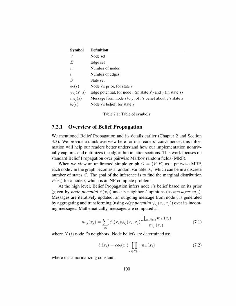
Symbol DefinitionV Node setE Edge setn Number of nodesl Number of edgesS State setφi(s) Node i’s prior, for state sψij(s

′, s) Edge potential, for node i (in state s′) and j (in state s)mij(s) Message from node i to j, of i’s belief about j’s state sbi(s) Node i’s belief, for state s

Table 7.1: Table of symbols

7.2.1 Overview of Belief PropagationWe mentioned Belief Propagation and its details earlier (Chapter 2 and Section3.3). We provide a quick overview here for our readers’ convenience; this infor-mation will help our readers better understand how our implementation nontriv-ially captures and optimizes the algorithm in latter sections. This work focuses onstandard Belief Propagation over pairwise Markov random fields (MRF).

When we view an undirected simple graph G = (V,E) as a pairwise MRF,each node i in the graph becomes a random variableXi, which can be in a discretenumber of states S. The goal of the inference is to find the marginal distributionP (xi) for a node i, which is an NP-complete problem.

At the high level, Belief Propagation infers node i’s belief based on its prior(given by node potential φ(xi)) and its neighbors’ opinions (as messages mji).Messages are iteratively updated; an outgoing message from node i is generatedby aggregating and transforming (using edge potential ψij(xi, xj)) over its incom-ing messages. Mathematically, messages are computed as:

mij(xj) =∑xi

φi(xi)ψij(xi, xj)

∏k∈N(i)mki(xi)

mji(xi)(7.1)

where N (i) node i’s neighbors. Node beliefs are determined as:

bi(xi) = cφi(xi)∏

k∈N(i)

mki(xi) (7.2)

where c is a normalizing constant.

100

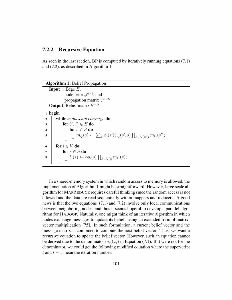
7.2.2 Recursive Equation

As seen in the last section, BP is computed by iteratively running equations (7.1)and (7.2), as described in Algorithm 1.

Algorithm 1: Belief PropagationInput : Edge E,

node prior φn×1, andpropagation matrix ψS×S

Output: Belief matrix bn×S

1 begin2 while m does not converge do3 for (i, j) ∈ E do4 for s ∈ S do5 mij(s)←

∑s′ φi(s

′)ψij(s′, s)

∏k∈N(i)\jmki(s

′);

6 for i ∈ V do7 for s ∈ S do8 bi(s)← cφi(s)

∏k∈N(i)mki(s);

In a shared-memory system in which random access to memory is allowed, theimplementation of Algorithm 1 might be straightforward. However, large scale al-gorithm for MAPREDUCE requires careful thinking since the random access is notallowed and the data are read sequentially within mappers and reducers. A goodnews is that the two equations (7.1) and (7.2) involve only local communicationsbetween neighboring nodes, and thus it seems hopeful to develop a parallel algo-rithm for HADOOP. Naturally, one might think of an iterative algorithm in whichnodes exchange messages to update its beliefs using an extended form of matrix-vector multiplication [75]. In such formulation, a current belief vector and themessage matrix is combined to compute the next belief vector. Thus, we want arecursive equation to update the belief vector. However, such an equation cannotbe derived due to the denominator mji(xi) in Equation (7.1). If it were not for thedenominator, we could get the following modified equation where the superscriptt and t− 1 mean the iteration number:

101

mij(xj)(t) =

∑xi

φi(xi)ψij(xi, xj)∏

k∈N(i)

mki(xi)(t−1)

=∑xi

ψij(xi, xj)bi(xi)

(t−1)

c

and thus

bi(xi)(t) = cφi(xi)

∏k∈N(i)

mki(xi)(t−1)

= φi(xi)∏

k∈N(i)

∑xk

ψki(xk, xi)bk(xk)(t−2) (7.3)

Notice that the recursive equation (7.3) is a fake, imaginary equation derivedfrom the assumption that equation (7.1) has no denominator. Although the recur-sive equation for the belief vector cannot be acquired by this way, there is a moredirect and intuitive way to get a recursive equation. We will describe how to get itin the next section.

7.2.3 Main Idea: Line graph Fixed Point(LFP)How can we get the recursive equation for the BP? What we need is a tractablerecursive equation well-suited for large scale MAPREDUCE framework. In thissection, we describe LINE GRAPH FIXED POINT (LFP), our formulation of BP interms of finding the fixed point of an induced graph from the original graph. Asseen in the last section, a recursive equation to update the beliefs cannot be ac-quired due to the denominator in the message update equation. Our main idea tosolve the problem is to flip the notion of the nodes and edges in the original graphand thus use the equation (7.1), without modification, as the recursive equationfor updating the ‘nodes’ in the new formulation. The ‘flipping’ means we con-sider an induced graph, called the line graph, whose nodes correspond to edgesin the original graph, and the two nodes in the induced graph are connected if thecorresponding edges in the original graph are incident. Notice that for each edge(i, j) in the original graph, two messages need to be defined since mij and mji aredifferent. Thus, the line graph should be directed, although the original graph isundirected. Formally, we define the ‘directed line graph’ as follows.

102

Definition 1 (Directed Line Graph) Given a directed graph G, its directed linegraph L(G) is a graph such that each node of L(G) represents an edge of G, andthere is an edge from vi to vj of L(G) if the corresponding edges ei and ej form alength-two directed path from ei to ej in G.

(a) Original graph (b) Directed graph (c) Directed line graph

Figure 7.1: Converting a undirected graph to a directed line graph. (a to b): replace aundirected edge with two directed edges. (b to c): for an edge (i, j) in (b), make a node(i, j) in (c). Make a directed edge from (i, j) to (k, l) in (c) if j = k and i 6= l. Therectangular nodes in (c) corresponds to edges in (b).

For example, see Figure 7.1 for a graph and its directed line graph. To converta undirected line graph G to a directed line graph L(G), we first convert G to adirected graph by converting each undirected edge to two directed edges. Then, adirected edge from vi to vj in L(G) is created if their corresponding edges ei andej form a directed path ei to ej in G.

Now, we derive the exact recursive equation on the line graph. Let G be theoriginal undirected graph with n nodes and l edges, and L(G) be the directed linegraph of G with 2l nodes as defined by Definition 1. The (i, j)th element L(G)i,jis defined to be 1 if the edge exist, or 0 otherwise. Let m be a 2l-vector whoseelement corresponding to the edge (i, j) inG contains the reverse directional mes-sage mji. The reason of this reverse directional message will be described soon.Let φ be a n-vector containing priors of each node. We build a 2l-vector ϕ asfollows: if the kth element ϕk of ϕ corresponds to an edge (i, j) in G, then set ϕkto φ(i). A standard matrix-vector multiplication with vector addition operation onL(G), m, ϕ is

m′ = L(G)×m+ ϕ

wherem′i =

∑nj=1 L(G)i,j ×mj + ϕi.

In the above equation, four operations are used to get the result vector:

1. combine2(L(G)i,j,mj): multiply L(G)i,j and mj .

103

2. combineAlli(y1, ..., yn): sum n multiplication results for node i.3. sumVector(ϕi, vaggr): add ϕi to the result vaggr of combineAll.4. assign(mi, oldvali, newvali): overwrite the previous value oldvali of mi

with the new value newvali to make m′i.

Now, we generalize the operators× and + to×G and +G, respectively, so thatthe four operations can be any functions of their arguments. In this generalizedsetting, the matrix-vector multiplication with vector addition operation becomes

m′ = L(G)×G m+G ϕ

wherem′i = assign(mi, oldvali,sumVector(ϕi,combineAlli({yj | j = 1..n, andyj =combine2(L(G)i,j,mj)}))).

An important observation is that the BP equation (7.1) can be representedby this generalized form of the matrix-vector multiplication with vector addition.For simplifying the explanation, we omit the edge potential ψij since it is a tinyinformation(e.g. 2 by 2 or 3 by 3 table), and the summation over xi, both of whichcan be accommodated easily. Then, the BP equation (7.1) is expressed by

m′ = L(G)T ×G m+G ϕ (7.4)m′′ = ChangeMessageDirection(m′) (7.5)

where

m′i = sumVector(ϕi,combineAlli({yj | j = 1..n, andyj =combine2(L(G)Ti,j,mj)}))

, the four operations are defined by

1. combine2(L(G)i,j,mj) = L(G)i,j ×mj

2. combineAlli(y1, ..., yn) =∏n

j=1 yj

3. sumVector(ϕi, vaggr) = ϕi × vaggr4. assign(mi, oldvali, newvali) = newvali/vali, and the ChangeMessageDirection function is defined by Algorithm 2. The

computed m′′ of equation (7.5) is the updated message which can be used as min the next iteration. Thus, our LINE GRAPH FIXED POINT (LFP) comprises run-ning the equation (7.4) and (7.5) iteratively until a fixed point, where the messagevector converges, is found.

104

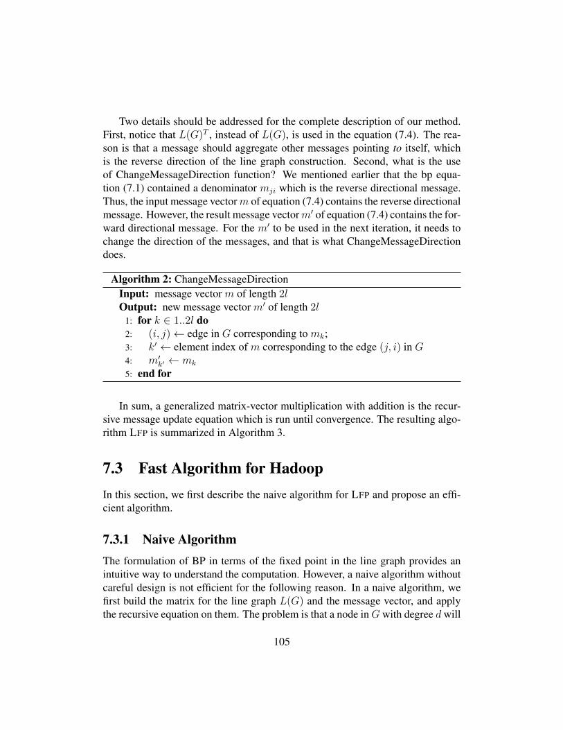
Two details should be addressed for the complete description of our method.First, notice that L(G)T , instead of L(G), is used in the equation (7.4). The rea-son is that a message should aggregate other messages pointing to itself, whichis the reverse direction of the line graph construction. Second, what is the useof ChangeMessageDirection function? We mentioned earlier that the bp equa-tion (7.1) contained a denominator mji which is the reverse directional message.Thus, the input message vectorm of equation (7.4) contains the reverse directionalmessage. However, the result message vectorm′ of equation (7.4) contains the for-ward directional message. For the m′ to be used in the next iteration, it needs tochange the direction of the messages, and that is what ChangeMessageDirectiondoes.

Algorithm 2: ChangeMessageDirectionInput: message vector m of length 2lOutput: new message vector m′ of length 2l

1: for k ∈ 1..2l do2: (i, j)← edge in G corresponding to mk;3: k′ ← element index of m corresponding to the edge (j, i) in G4: m′k′ ← mk

5: end for

In sum, a generalized matrix-vector multiplication with addition is the recur-sive message update equation which is run until convergence. The resulting algo-rithm LFP is summarized in Algorithm 3.

7.3 Fast Algorithm for HadoopIn this section, we first describe the naive algorithm for LFP and propose an effi-cient algorithm.

7.3.1 Naive AlgorithmThe formulation of BP in terms of the fixed point in the line graph provides anintuitive way to understand the computation. However, a naive algorithm withoutcareful design is not efficient for the following reason. In a naive algorithm, wefirst build the matrix for the line graph L(G) and the message vector, and applythe recursive equation on them. The problem is that a node inGwith degree dwill

105

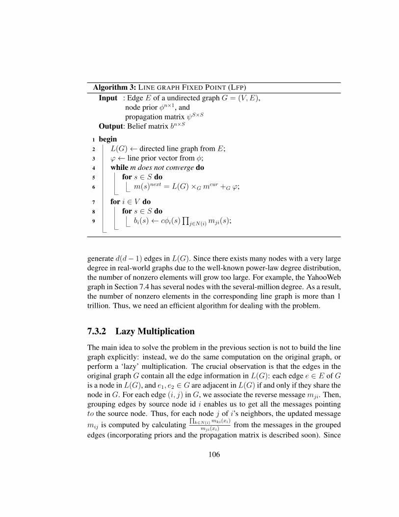
Algorithm 3: LINE GRAPH FIXED POINT (LFP)Input : Edge E of a undirected graph G = (V,E),

node prior φn×1, andpropagation matrix ψS×S

Output: Belief matrix bn×S

1 begin2 L(G)← directed line graph from E;3 ϕ← line prior vector from φ;4 while m does not converge do5 for s ∈ S do6 m(s)next = L(G)×G mcur +G ϕ;

7 for i ∈ V do8 for s ∈ S do9 bi(s)← cφi(s)

∏j∈N(i)mji(s);

generate d(d− 1) edges in L(G). Since there exists many nodes with a very largedegree in real-world graphs due to the well-known power-law degree distribution,the number of nonzero elements will grow too large. For example, the YahooWebgraph in Section 7.4 has several nodes with the several-million degree. As a result,the number of nonzero elements in the corresponding line graph is more than 1trillion. Thus, we need an efficient algorithm for dealing with the problem.

7.3.2 Lazy Multiplication

The main idea to solve the problem in the previous section is not to build the linegraph explicitly: instead, we do the same computation on the original graph, orperform a ‘lazy’ multiplication. The crucial observation is that the edges in theoriginal graph G contain all the edge information in L(G): each edge e ∈ E of Gis a node in L(G), and e1, e2 ∈ G are adjacent in L(G) if and only if they share thenode in G. For each edge (i, j) in G, we associate the reverse message mji. Then,grouping edges by source node id i enables us to get all the messages pointingto the source node. Thus, for each node j of i’s neighbors, the updated messagemij is computed by calculating

∏k∈N(i)mki(xi)

mji(xi)from the messages in the grouped

edges (incorporating priors and the propagation matrix is described soon). Since

106

we associate the reverse message for each edge, the output triple (src, dst, reversemessage) is (j, i,mij).

An issue in computing∏k∈N(i)mki(xi)

mji(xi)is that a straightforward implementa-

tion requires N(i)(N(i) − 1) multiplication which is prohibitively large. How-ever, we decrease the number of multiplication to 2N(i) by first computingt =

∏k∈N(i)mki(s

′), and for each j ∈ N(i) computing t/mji(s′).

The only remaining pieces of the computation is to incorporate the prior φ andthe propagation matrix ψ. The propagation matrix ψ is a tiny bit of information,so it can be sent to every reducer by a variable passing functionality of HADOOP.The prior vector φ can be large, since the length of the vector can be the num-ber of nodes in the graph. In the HADOOP algorithm, we also group the φ bythe node id: each node prior is grouped together with the edges(messages) whosesource id is the node id. Algorithm 4 shows the high-level algorithm of HADOOP

LINE GRAPH FIXED POINT (HA-LFP). Algorithm 5 shows the BP message ini-tialization algorithm which requires only a Map function. Algorithm 6 showsthe HADOOP algorithm for the message update which implements the algorithmdescribed above. After the messages converge, the final belief is computed byAlgorithm 7.

Algorithm 4: HADOOP LINE GRAPH FIXED POINT (HA-LFP)Input : Edge E of a undirected graph G = (V,E),

node prior φn×1, andpropagation matrix ψS×S

Output: Belief matrix bn×S

1 begin2 Initialization(); // Algorithm 53 while m does not converge do4 MessageUpdate(); // Algorithm 6

5 BeliefComputation(); // Algorithm 7

7.3.3 Analysis

We analyze the time and the space complexity of HA-LFP. The main result is thatone iteration of the message update on the line graph has the same complexity as

107

Algorithm 5: HA-LFP InitializationInput : Edge E = {(idsrc, iddst)},

Set of states S = {s1, ..., sp}Output: Message Matrix M = {(idsrc, iddst,mdst,src(s1), ...,mdst,src(sp))}

1 Initialization-Map(Key k, Value v);2 begin3 Output((k, v), ( 1

|S| , ..., 1|S| )); // (k: idsrc, v: iddst)

one matrix-vector multiplication on the original graph. In the lemmas below, Mis the number of machines.

Lemma 1 (Time Complexity of HA-LFP ) One iteration of HA-LFP takesO(V+E

Mlog V+E

M) time. It could take O(V+E

M) time if HADOOP uses only hash-

ing, not sorting, on its shuffling stage.

Proof 1 Notice that the number of states is usually very small(2 or 3), thus canbe considered as a constant. Assuming uniform distribution of data to machines,the time complexity is dominated by the MessageUpdate job. Thanks to the ‘lazymultiplication’ described in the previous section, both Map and Reduce takes lin-ear time to the input. Thus, the time complexity is O(V+E

Mlog V+E

M), which is the

sorting time for V+EM

records. It could be O(V+EM

), if HADOOP performs onlyhashing without sorting on its shuffling stage.

A similar results holds for space complexity.Lemma 2 (Space Complexity of HA-LFP ) HA-LFP requires O(V +E) space.

Proof 2 The prior vector requires O(V ) space, and the message matrix requiresO(2E) space. Since the number of edges is greater than the number of nodes,HA-LFP requires O(V + E) space, in total.

7.4 ExperimentsIn this section, we present experimental results to answer the following questions:

Q1 How fast is HA-LFP, compared to a single-machine version?

Q2 How does HA-LFP scale up with the number of machines?

Q3 How does HA-LFP scale up with the number of edges?

108

Graph Nodes Edges File Desc.

YahooWeb 1,413 M 6,636 M 0.24 TB page-pageTwitter’10 104 M 3,730 M 0.13 TB person-personTwitter’09 63 M 1,838 M 56 GB person-personKronecker 177 K 1,977 M 25 GB synthetic

120 K 1,145 M 13.9 GB59 K 282 M 3.3 GB

VoiceCall 30 M 260 M 8.4 GB who calls whomSMS 7 M 38 M 629 MB who sends to whom

Table 7.2: Order and size of networks.

We performed experiments in the M45 HADOOP cluster by Yahoo!. The clus-ter has total 480 machines with 1.5 Petabyte total storage and 3.5 Terabyte mem-ory. The single-machine experiment was done in a machine with 3 Terabyte ofdisk and 48 GB memory. The single-machine BP algorithm is a scaled-up versionof a memory-based BP which reads all the nodes, not the edges, into a memory.That is, the single-machine BP loads only the node information into a memory,but it reads the edges sequentially from the disk for every message update, insteadof loading all the edges into a memory once for all.

The graphs we used in our experiments at Section 7.4 and 7.5 are summarizedin Table 7.2 1:

• YahooWeb: web pages and their links, crawled by Yahoo! at year 2002.• Twitter: social network(who follows whom) extracted from Twitter, at June

2010 and Nov 2009.• Kronecker[91]: synthetic graph with similar properties as real-world

graphs.• VoiceCall: phone call records(who calls whom) during Dec. 2007 to Jan.

2008 from an anonymous phone service provider.• SMS: short message service records(who sends to whom) during Dec. 2007

to Jan. 2008 from an anonymous phone service provider.

1 YahooWeb: released under NDA.Twitter: http://www.twitter.comKronecker: [91]VoiceCall, SMS: not public data.

109

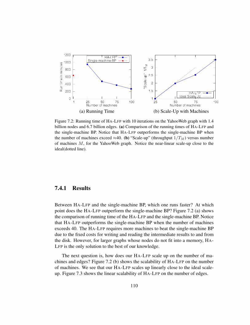
(a) Running Time (b) Scale-Up with Machines

Figure 7.2: Running time of HA-LFP with 10 iterations on the YahooWeb graph with 1.4billion nodes and 6.7 billion edges. (a) Comparison of the running times of HA-LFP andthe single-machine BP. Notice that HA-LFP outperforms the single-machine BP whenthe number of machines exceed ≈40. (b) “Scale-up” (throughput 1/TM ) versus numberof machines M , for the YahooWeb graph. Notice the near-linear scale-up close to theideal(dotted line).

7.4.1 Results

Between HA-LFP and the single-machine BP, which one runs faster? At whichpoint does the HA-LFP outperform the single-machine BP? Figure 7.2 (a) showsthe comparison of running time of the HA-LFP and the single-machine BP. Noticethat HA-LFP outperforms the single-machine BP when the number of machinesexceeds 40. The HA-LFP requires more machines to beat the single-machine BPdue to the fixed costs for writing and reading the intermediate results to and fromthe disk. However, for larger graphs whose nodes do not fit into a memory, HA-LFP is the only solution to the best of our knowledge.

The next question is, how does our HA-LFP scale up on the number of ma-chines and edges? Figure 7.2 (b) shows the scalability of HA-LFP on the numberof machines. We see that our HA-LFP scales up linearly close to the ideal scale-up. Figure 7.3 shows the linear scalability of HA-LFP on the number of edges.

110

Figure 7.3: Running time of 1 iterations of message update in HA-LFP on Kroneckergraphs. Notice that the running time scales-up linear to the number of edges.

7.4.2 Discussion

Based on the experimental results, what are the advantages of HA-LFP? In whatsituations should it be used? For a small graph whose nodes and edges fit inthe memory, the single-machine BP is recommended since it runs faster. For amedium-to-large graph whose nodes fit in the memory but the edges do not fit inthe memory, HA-LFP gives the reasonable solution since it runs faster than thesingle-machine BP. For a very large graph whose nodes do not fit in the memory,HA-LFP is the only solution. We summarize the advantages of the HA-LFP here:

• Scalability: HA-LFP is the only solution when the nodes information cannot fit in memory. Moreover, HA-LFP scales up near-linearly.

• Running Time: Even for a graph whose node information fits into a mem-ory, HA-LFP ran 2.4 times faster.

• Fault Tolerance: HA-LFP enjoys the fault tolerance that HADOOP pro-vides: data are replicated, and the failed programs due to machine errorsare restarted in working machines.

7.5 Analysis of Real Graphs

In this section, we analyze real-world graphs using HA-LFP and report findings.

111

7.5.1 HA-LFP on YahooWeb

Given a web graph, how can we separate the educational(‘good’) web pages fromthe adult(‘bad’) web pages? Manually investigating billions of web pages wouldtake so much time and efforts. In this section, we show how to do it using HA-LFP. We use a simple heuristic to set priors: the web pages which contain ‘edu’have high goodness prior(0.95), and the web pages which contain either ‘sex’,‘adult’, or ‘porno’ have low goodness prior(0.05). Among 11.8 million web pagescontaining sexually explicit keywords, we keep 10% of the pages as a validationset (goodness prior 0.5), and use the rest 90% as a training set by setting thegoodness prior 0.05. Also, among 41.7 million web pages containing ‘edu’, werandomly sample 11.8 million web pages, so that the number equals with thatof adult pages given prior, and use 10% as a validation set(goodness prior 0.5),and use the rest 90% as a training set(goodness prior 0.95). The edge potentialfunction is given by Table 7.3. It is given by our observation that good pages tendto point to other good pages, while bad pages might point to good pages, as wellas bad pages, to boost their ranking in web search engines.

Good BadGood 1-ε ε

Bad 0.5 0.5

Table 7.3: Edge potential for the YahooWeb. ε is set to 0.05 in the experiments. Goodpages point to other good pages with high probability. Bad pages point to bad pages, butalso good pages with equal chances, to boost their rank in web search engines.

Figure 7.4 shows the HA-LFP scores and the number of pages in the test sethaving such scores. Notice that almost all the pages with LFP score less than 0.9in our test data contain adult web sites. Thus, the LFP score 0.9 can be used as adecision boundary for adult web pages.

112

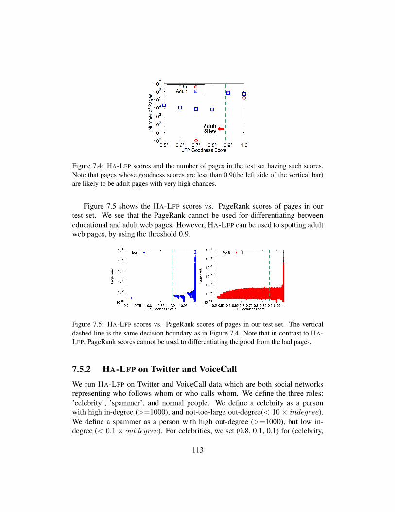
Figure 7.4: HA-LFP scores and the number of pages in the test set having such scores.Note that pages whose goodness scores are less than 0.9(the left side of the vertical bar)are likely to be adult pages with very high chances.

Figure 7.5 shows the HA-LFP scores vs. PageRank scores of pages in ourtest set. We see that the PageRank cannot be used for differentiating betweeneducational and adult web pages. However, HA-LFP can be used to spotting adultweb pages, by using the threshold 0.9.

Figure 7.5: HA-LFP scores vs. PageRank scores of pages in our test set. The verticaldashed line is the same decision boundary as in Figure 7.4. Note that in contrast to HA-LFP, PageRank scores cannot be used to differentiating the good from the bad pages.

7.5.2 HA-LFP on Twitter and VoiceCallWe run HA-LFP on Twitter and VoiceCall data which are both social networksrepresenting who follows whom or who calls whom. We define the three roles:’celebrity’, ’spammer’, and normal people. We define a celebrity as a personwith high in-degree (>=1000), and not-too-large out-degree(< 10 × indegree).We define a spammer as a person with high out-degree (>=1000), but low in-degree (< 0.1 × outdegree). For celebrities, we set (0.8, 0.1, 0.1) for (celebrity,

113

spammer, normal) prior probabilities. For spammers, we set (0.1, 0.8, 0.1) for(celebrity, spammer, normal) prior probabilities. The edge potential function isgiven by Table 7.4. It encodes our observation that celebrities tend to follownormal persons the most, spammers follow other spammers or normal persons,and normal persons follow other normal persons or celebrities.

Celebrity Spammer NormalCelebrity 0.1 0.05 0.85Spammer 0.1 0.45 0.45Normal 0.35 0.05 0.6

Table 7.4: Edge potential for the Twitter and VoiceCall graph

Figure 7.6 shows the HA-LFP scores of people in the Twitter and VoiceCalldata. There are two clusters in both of the data. The large cluster starting from the‘Normal’ vertex contains high degree nodes, and the small cluster below the largecluster contains low degree nodes.

(a) Twitter (b) VoiceCall

Figure 7.6: HA-LFP scores of people in the Twitter and VoiceCall data. The points repre-sent the scores of the final beliefs in each state, forming simplex in 3-dimensional spacewhose axes are the red lines that meet at the center(origin). Notice that people seem toform two groups, in both datasets, despite the fact that the two datasets are completely ofdifferent nature.

7.5.3 Finding Roles And AnomaliesIn the experiments of previous sections, we used several classes(‘bad’ web sites,‘spammers’, ‘celebrities’, etc.) of nodes. The question is, how can we find classesof a given graph? Finding out such classes is important for BP since it helps to

114

set reasonable priors which could lead to quick convergence. Here, we analyzereal world graphs using the PEGASUS package [75] and give observations onthe patterns and anomalies, which could potentially help determine the classes.We focus on the structural properties of graphs, such as degree and connectedcomponent distributions.

115

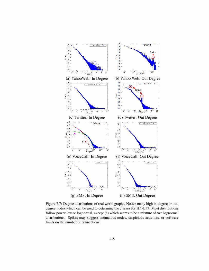
(a) YahooWeb: In Degree (b) Yahoo Web: Out Degree

(c) Twitter: In Degree (d) Twitter: Out Degree

(e) VoiceCall: In Degree (f) VoiceCall: Out Degree

(g) SMS: In Degree (h) SMS: Out Degree

Figure 7.7: Degree distributions of real world graphs. Notice many high in-degree or out-degree nodes which can be used to determine the classes for HA-LFP. Most distributionsfollow power-law or lognormal, except (e) which seems to be a mixture of two lognormaldistributions. Spikes may suggest anomalous nodes, suspicious activities, or softwarelimits on the number of connections.

116

Using Degree Distributions

We first show the degree distributions of real world graphs in Figure 7.7. No-tice that there are nodes with very high in or out degrees, which gives valuableinformation for setting priors.

Observation 1 (High In or Out Degree Nodes) The nodes with high in-degreecan have a high prior for ‘celebrity’, and the nodes with high out-degree but lowin-degree can have a high prior for ‘spammer’.

Most of the degree distributions in Figure 7.7 follow power law or log-normal.The VoiceCall in degree distribution(Figure 7.7 (e)) is different from other distri-butions since it contains mixture of distributions:

Observation 2 (Mixture of Lognormals in Degree Distribution) VoiceCall indegree distributions in Figure 7.7 seems to comprise two lognormal distributionsshown in D1(red color) and D2(green color).

Another observation is that there are several anomalous spikes in the degreedistributions in Figure 7.7 (b) and (d).

Observation 3 (Spikes in Degree Distribution) There is a huge spike at the outdegree 1200 of YahooWeb data in Figure 7.7 (b). They came from online marketpages from Germany, where the pages are linked to each other and forming linkfarms. Two outstanding spikes are also observed at the out degree 20 and 2001 ofTwitter data in Figure 7.7 (d). The reason seems to be a hard limit in the maximumnumber of people to follow.

Finally, we study the highest degrees that are beyond the power-law or lognor-mal cutoff points using rank plot. Figure 7.8 shows the top 1000 highest in andout degrees and its rank(from 1 to 1000) which we summarize in the followingobservation.

Observation 4 (Tilt in Rank Plot) The out degree rank plot of Twitter data inFigure 7.8 (b) follows a power law with a single exponent. The in degree rankplot, however, comprises two fitting lines with a tilting point around rank 240. Thetilting point divides the celebrities in two groups: super-celebrities (e.g., possibly,of international caliber) and plain celebrities (possibly, of national caliber).

117

(a) In degree vs. Rank (b) Out degree vs. Rank

Figure 7.8: Degree vs. Rank. in Twitter Jun. 2010 data. Notice the change of slopearound the tilting point in (a). The point can be used to distinguishing super-celebrities(e.g., of international caliber) versus plain celebrities (of national or regional caliber).

Using Connected Component Distributions.

The distributions of the sizes of connected components in a graph informs us ofthe connectivity of the nodes (component size vs. number of components havingthat size). When these distributions are plotted over time, we may observe whencertain nodes participate in various activities — patterns such as periodicity oranomalous deviations from such patterns can generate important insights.

Figure 7.9 shows the temporal connected component distribution of the Voice-Call (who-calls-whom) data, where each data point was computed using one day’sworth of data (i.e., a one-day snapshot).

Observation 5 (Periodic Dips and Surges) Every Sunday, we see a dip in thesize of the giant connected component (largest component), and an accompanyingsurge in the number of connected components for the day. We may infer that“business” phone numbers (nodes) are those that are regularly active during workdays but not weekends, and characterize these them as under the “business” classin our algorithm.

118

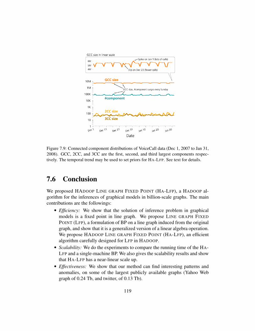
Figure 7.9: Connected component distributions of VoiceCall data (Dec 1, 2007 to Jan 31,2008). GCC, 2CC, and 3CC are the first, second, and third largest components respec-tively. The temporal trend may be used to set priors for HA-LFP. See text for details.

7.6 ConclusionWe proposed HADOOP LINE GRAPH FIXED POINT (HA-LFP), a HADOOP al-gorithm for the inferences of graphical models in billion-scale graphs. The maincontributions are the followings:• Efficiency: We show that the solution of inference problem in graphical

models is a fixed point in line graph. We propose LINE GRAPH FIXED

POINT (LFP), a formulation of BP on a line graph induced from the originalgraph, and show that it is a generalized version of a linear algebra operation.We propose HADOOP LINE GRAPH FIXED POINT (HA-LFP), an efficientalgorithm carefully designed for LFP in HADOOP.

• Scalability: We do the experiments to compare the running time of the HA-LFP and a single-machine BP. We also gives the scalability results and showthat HA-LFP has a near-linear scale up.

• Effectiveness: We show that our method can find interesting patterns andanomalies, on some of the largest publicly available graphs (Yahoo Webgraph of 0.24 Tb, and twitter, of 0.13 Tb).

119

Algorithm 6: HA-LFP Message UpdateInput : Set of states S = {s1, ..., sp},

Current Message Matrix M cur ={(sid, did,mdid,sid(s1), ...,mdid,sid(sp))},Prior Matrix Φ = {(id, φid(s1), ..., φid(sp))},Propagation Matrix ψ

Output: Updated Message MatrixMnext = {(idsrc, iddst,mdst,src(s1), ...,mdst,src(sp))}

1 MessageUpdate-Map(Key k, Value v);2 begin3 if (k, v) is of type M then4 Output(k, v); // (k: sid, v: did,mdid,sid(s1), ...,mdid,sid(sp))5 else if (k, v) is of type Φ then6 Output(k, v); // (k: id, v: φid(s1), ..., φid(sp))7

8 MessageUpdate-Reduce(Key k, Value v[1..r]);9 begin

10 temps[1..p]← [1..1];11 saved prior ←[ ];12 HashTable<int, double[1..p]> h;13 foreach v ∈ v[1..r] do14 if (k, v) is of type Φ then15 saved prior[1..p]← v;16 else if (k, v) is of type M then17 (did,mdid,sid(s1), ...,mdid,sid(sp))← v;18 h.add(did, (mdid,sid(s1), ...,mdid,sid(sp)));19 foreach i ∈ 1..p do20 temps[i] = temps[i]×mdid,sid(si);

21

22 foreach (did, (mdid,sid(s1), ...,mdid,sid(sp))) ∈ h do23 outm[1..p]← 0;24 foreach u ∈ 1..p do25 foreach v ∈ 1..p do26 outm[u] =

outm[u] + saved prior[v]ψ(v, u)temps[v]/mdid,sid(sv);

27 Output(did, (sid, outm[1], ..., outm[p]));

120

Algorithm 7: HA-LFP Belief ComputationInput : Set of states S = {s1, ..., sp},

Current Message Matrix M cur ={(sid, did,mdid,sid(s1), ...,mdid,sid(sp))},Prior Matrix Φ = {(id, φid(s1), ..., φid(sp))}

Output: Belief Vector b = {(id, bid(s1), ..., bid(sp))}1 BeliefComputation-Map(Key k, Value v);2 begin3 if (k, v) is of type M then4 Output(k, v); // (k: sid, v: did,mdid,sid(s1), ...,mdid,sid(sp))5 else if (k, v) is of type Φ then6 Output(k, v); // (k: id, v: φid(s1), ..., φid(sp))7

8 BeliefComputation-Reduce(Key k, Value v[1..r]);9 begin

10 b[1..p]← [1..1];11 foreach v ∈ v[1..r] do12 if (k, v) is of type Φ then13 prior[1..p]← v;14 foreach i ∈ 1..p do15 b[i] = b[i]× prior[i];16 else if (k, v) is of type M then17 (did,mdid,sid(s1), ...,mdid,sid(sp))← v;18 foreach i ∈ 1..p do19 b[i] = b[i]×mdid,sid(si);

20

21 Output(k, (b[1], ..., b[p]));

121

122

Chapter 8

Unifying Guilt-by-AssociationMethods: Theories &Correspondence

If several friends of Smith have committed petty thefts, what would you say aboutSmith? Most people would not be surprised if Smith is a hardened criminal, withmore than petty thefts on his record. Guilt-by-association methods can help uscombine weak signals to derive stronger ones. We leveraged this core idea in ourPolonium work to detect malware (Chapter 4), and in our Apolo system to findrelevant nodes to explore (Chapter 5).

The focus of this work is to compare and contrast several very successful,guilt-by-association methods: RWR (Random Walk with Restarts) ; SSL (Semi-Supervised Learning); and Belief Propagation (Belief Propagation). RWR is themethod behind Google’s multi-billion dollar PageRank algorithm. SSL is appli-cable when we have labeled and unlabeled nodes in a graph. BP is a methodfirmly based on Bayesian reasoning, with numerous successful applications (eg.image restoration and error-correcting algorithms). Which of the three methodsshould one use? Does the choice make a difference? Which method converges,and when?

Our main contributions are two-fold: (a) theoretically, we prove that all themethods result in a similar matrix inversion problem; (b) for practical applica-tions, we developed FABP, a fast algorithm that yields 2× speedup compared to

Chapter adapted from work appeared at PKDD 2011 [86]

123

Belief Propagation, while achieving equal or higher accuracy, and is guaranteed toconverge. We demonstrate these benefits using synthetic and real datasets, includ-ing YahooWeb, one of the largest graphs ever studied with Belief Propagation.

8.1 Introduction

Network effects are very powerful, resulting even in popular proverbs (“birds ofa feather flock together”). In social networks, obese people tend to have obesefriends [34], happy people tend to make their friends happy too [48], and in gen-eral, people tend to associate with like-minded friends, with respect to politics,hobbies, religion, etc. Thus, knowing the types of a few nodes in a network, wewould have good chances to guess the types of the rest of the nodes.

Informally, the problem definition is as follows:Given: a graph withN nodes andM edges; n+ and n− nodes labeled as members

of the positive and negative class respectively

Find: the class memberships of the rest of the nodes, assuming that neighborsinfluence each other

The influence can be “homophily”, meaning that nearby nodes have similar labels;or “heterophily”, meaning the reverse (e.g., talkative people tend to prefer silentfriends, and vice-versa). Most methods we cover next support only homophily,but our proposed FABP method, improved on Belief Propagation, can triviallyhandle both cases.

Homophily appears in numerous settings, for example (a) PersonalizedPageRank: if a user likes some pages, she would probably like other pages thatare heavily connected to her favorites. (b) Recommendation systems: in a user× product matrix, if a user likes some products (i.e., members of positive class),which other products should get positive scores? (c) Accounting and calling-cardfraud: if a user is dishonest, his/her contacts are probably dishonest too.

There are several, closely related methods that address the homophily prob-lem, and some that address both homophily and heterophily. We focus on three ofthem: Personalized PageRank (a.k.a. “Personalized Random Walk with Restarts”,or just RWR); Semi-Supervised Learning (SSL); and Belief Propagation (BeliefPropagation). How are these methods related? Are they identical? If not, whichmethod gives the best accuracy? Which method has the best scalability?

These questions are exactly the focus of this work. We contribute by answer-ing the above questions, plus a fast algorithm inspired by our theoretical analysis:

124

• Theory & Correspondences: the methods are closely related, but not iden-tical.

• Algorithm & Convergence: we propose FABP, a fast, accurate and scalablealgorithm, and provide the conditions under which it converges.

• Implementation & Experiments: finally, we propose a HADOOP-based algo-rithm, that scales to billion-node graphs, and we report experiments on oneof the largest graphs ever studied in the open literature. Our FABP methodachieves about 2× better runtime.

8.2 Related WorkAll three alternatives are very popular, with numerous papers using or improvingthem. Here, we survey the related work for each method.

Random Walk with Restarts (RWR) RWR is the method underlyingGoogle’s classic PageRank algorithm [22]. RWR’s many variations include Per-sonalized PageRank [57], lazy random walks [103], and more[144, 113]. Relatedmethods for node-to-node distance (but not necessarily guilt-by-association) in-clude [85], parameterized by escape probability and round-trip probability.

Semi-supervised learning (SSL) According to conventional categorization,SSL approaches are divided into four categories [159]: low-density separationmethods, graph-based methods, methods for changing the representation, andco-training methods. The principle behind SSL is that unlabeled data can helpus decide the “metric” between data points and improve models’ performance. Avery recent use of SSL for multi-class settings has been proposed in [66].

Belief Propagation (BP) Here, we focus on standard Belief Propagation andwe study how its parameter choices help accelerate the algorithm, and how to im-plement the method on top of HADOOP [2] (open-source MapReduce implemen-tation). This focus differentiates our work from existing research which speedsup Belief Propagation by exploiting the graph structure [33, 114] or the order ofmessage propagation [52].

Summary None of the above papers show the relationships between the threemethods, or discuss the parameter choices (e.g., homophily scores). Table 8.1

125

qualitatively compares the methods. All methods are scalable. Belief Propaga-tion supports heterophily, but there is no guarantee on convergence. Our FABPalgorithm improves on it to provide convergence.

Table 8.1: Qualitative comparison of ‘guilt-by-association’ (GBA) methods.

GBA Method Heterophily Scalability ConvergenceRWR No Yes YesSSL No Yes YesBP Yes Yes ?FABP Yes Yes Yes

8.3 Theorems and CorrespondencesIn this section we present the three main formulas that show the similarity ofthe following methods: (binary) Belief Propagation and specifically our proposedapproximation, the linearized BP (FABP), the Gaussian BP (GAUSSIANBP), thePersonalized RWR (RWR), and semi-supervised learning (SSL).

For the homophily case, all the above methods are similar in spirit, and closelyrelated to diffusion processes: the n+ nodes that belong to class “+” (say, “green”),act as if they taint their neighbors (diffusion) with green color, and similarly dothe negative nodes with, say, red color. Depending on the strength of homophily,or equivalently the speed of diffusion of the color, eventually we have green-ishneighborhoods, red-ish neighborhoods, and bridge-nodes (half-red, half-green).

As we show next, the solution vectors for each method obey very similar equa-tions: they all involve a matrix inversion, where the matrix consists of a diagonalmatrix plus a weighted or normalized version of the adjacency matrix. Table 8.2shows the resulting equations, carefully aligned to highlight the correspondences.

Next we give the equivalence results for all 3 methods, and the convergenceanalysis for FABP. At this point we should mention that work on the convergenceof a variant of Belief Propagation, Gaussian Belief Propagation, is done in [96]and [151]. The reasons that we focus on Belief Propagation are that (a) it has asolid, Bayesian foundation, and (b) it is more general than the rest, being able tohandle heterophily (as well as multiple-classes, that we don’t elaborate here).

In the following discussion, we use the symbols that are defined in Table 8.3.The detailed proofs of the Theorems and Lemmas can be found in Appendix B,while the preliminary analysis is given in Appendix A. Notice that in FABP, the

126

Method matrix unknown knownRWR [I − cAD−1]× x = (1− c) ySSL [I + α(D−A)]× x = yGaussian BP = SSL [I + α(D−A)]× x = yFABP [I + aD− c′A]× bh = φh

Table 8.2: Main results, to illustrate correspondence. Matrices (in capital and bold) aren×n; vectors (lower-case bold) are n×1 column vectors, and scalars (in lower-case plainfont) typically correspond to strength of influence. Detailed definitions: in the text.

Definition Explanationn #nodesA n× n sym. adj. matrixD n× n diag. matrix of degrees Dii =

∑j Aij and Dij = 0 for i 6= j

I n× n identity matrix“about-half” beliefs b = n× 1 BP’s belief vector

b− 0.5 b(i){> 0.5, < 0.5} means i ∈ {“+”, “-”} classbh

b(i) = 0 means i is unclassified (neutral)φh “about-half” prior, φ− 0.5 φ = n× 1 BP’s prior belief vector

“about-half” homophily vector h = ψ(“+”,“+”): entry of BP propagation matrixh− 0.5 h→ 0 : strong heterophilyhh

h→ 1 : strong homophily

Table 8.3: Symbols and definitions. Matrices in bold capital font; vectors in bold lower-case; scalars in plain font)

notion of the propagation matrix is represented by the “about-half” homophilyfactor.

Theorem 1 (FABP) The solution to belief propagation can be approximated bythe linear system

[I + aD− c′A]bh = φh (8.1)

where a = 4h2h/(1− 4h2h), and c′ = 2hh/(1− 4h2h). The quantities hh, φh and bh

are defined in Table 8.3, and depend on the strength of homophily. Specifically,φh corresponds to the prior beliefs of the nodes and φh(i) = 0 for the nodes thatwe have no information about; bh corresponds to the vector of our final beliefsfor each node.Proof 3 See Appendix B. QED

Lemma 1 (Personalized RWR) The linear system for RWR given an observation

127

y, is described by the following formula:

[I− cAD−1]x = (1− c)y . (8.2)

where 1− c is the restart probability, c ∈ [0, 1].

Proof 4 See [58], [144]. QEDSimilarly to the BP case above, y corresponds to the prior beliefs for each node,with the small difference that yi = 0 means that we know nothing about node i,while a positive score yi > 0 means that the node belongs to the positive class(with the corresponding strength).Lemma 2 (SSL and Gaussian BP) Suppose we are given l labeled nodes(xi, yi), i = 1, . . . , l, yi ∈ {0, 1}, and u unlabeled nodes (xl+1, ..., xl+u). Thesolution to a Gaussian BP and SSL problem is given by the linear system:

[α(D−A) + I]x = y (8.3)

where α is related to the coupling strength (homophily) of neighboring nodes.

Proof 5 See [151][159] and Appendix B. QEDAs before, y represents the labels of the labeled nodes and, thus, it is related tothe prior beliefs in BP; x corresponds to the labels of all the nodes or equivalentlythe final beliefs in BP.

Lemma 3 (R-S correspondence) On a regular graph (i.e., all nodes have thesame degree d), RWR and SSL can produce identical results if

α =c

(1− c)d(8.4)

That is, we need to align carefully the homophily strengths α and c.

Proof 6 See Appendix B. QEDIn an arbitrary graph the degrees are different, but we can still make the two meth-ods give the same results if we make α be different for each node i, that is αi.Specifically, the elements αi should be c

(1−c)di for node i, with degree di.

8.3.1 Arithmetic ExamplesHere we illustrate that SSL and RWR give closely related solutions. We set α tobe α = c/((1− c) ∗ d)) (where d is the average degree).

128

Figure 8.1 shows the scatter-plot: each red star (xi, yi) corresponds to a node,say, node i; the coordinates are the RWR and SSL scores, respectively. Theblue circles correspond to the perfect identity, and thus are on the 45-degree line.Figure 8.1(a) has three major groups, corresponding to the ’+’-labeled, the un-labeled, and the ’-’-labeled nodes (from top-right to bottom-left, respectively).Figure 8.1(b) shows a magnification of the central part (the unlabeled nodes). No-tice that the red stars are close to the 45-degree line. The conclusion is that (a) theSSL and RWR scores are similar, and (b) the rankings are the same: whichevernode is labeled as “positive” by SSL, gets a high score by RWR, and conversely.

Figure 8.1: Scatter plot showing the similarities between SSL and RWR. SSL vs RWRscores, for the nodes of a random graph; blue circles (ideal, perfect equality) and red stars(real). Right: a zoom-in of the left. Most red stars are on or close to the diagonal: the twomethods give similar scores, and identical assignments to positive/negative classes.

8.4 Analysis of ConvergenceHere we study the sufficient, but not necessary conditions for which our methodFABP converges. The implementation details of FABP are described in the up-coming Section 8.5. Lemmas 4, 5, and 8.8 give the convergence conditions.

All our results are based on the power expansion that results from the inversionof a matrix of the form I−W; all the methods undergo this process, as we show inTable 8.2. Specifically, we need the inverse of the matrix I+ aD− c′A = I−W,which is given the expansion:

(I−W)−1 = I + W + W2 + W3 + ... (8.5)

and the solution of the linear system is given by the formula

(I−W)−1φh = φh + W · φh + W · (W · φh) + ... (8.6)

129

This method is fast since the computation can be done in iterations, each one ofwhich consists of a sparse-matrix/vector multiplication. This is referred to as thePower Method. However, the Power Method does not always converge. In thissection we examine its convergence conditions.

Lemma 4 (Largest eigenvalue) The series∞∑k=0

|W|k =∞∑k=0

|c′A− aD|k con-

verges iff λ(W) < 1, where λ(W) is the magnitude of the largest eigenvalueof W.Given that the computation of the largest eigenvalue is non-trivial, we suggestusing one of the following lemmas, which give a closed form for computing the“about-half” homophily factor, hh.

Lemma 5 (1-norm) The series∞∑k=0

|W|k =∞∑k=0

|c′A− aD|k converges if

hh <1

2(1 + maxj (djj))(8.7)

where djj are the elements of the diagonal matrix D.

Proof 7 The proof is based on the fact that the power series converges if the 1-norm, or equivalently the∞-norm, of the symmetric matrix W is smaller than 1.The detailed proof can be found in Appendix C. QED

Lemma 6 (Frobenius norm) The series∞∑k=0

|W|k =∞∑k=0

|c′A− aD|k con-

verges if

hh <

√−c1 +

√c21 + 4c2

8c2(8.8)

where c1 = 2 +∑i

dii and c2 =∑i

d2ii − 1.

Proof 8 This upper bound for hh is obtained when we consider the Frobenius

norm of matrix W and we solve the inequality ‖W ‖F=

√√√√ n∑i=1

n∑j=1

|Wij|2 < 1

with respect to hh. We omit the detailed proof. QEDFormula 8.8 is preferable over 8.7 when the degrees of the graph’s nodes demon-strate considerable standard deviation. The 1-norm yields small hh for very big

130

Dataset #nodes #edgesYahooWeb 1,413,511,390 6,636,600,779Kronecker 1 177,147 1,977,149,596Kronecker 2 120,552 1,145,744,786Kronecker 3 59,049 282,416,200Kronecker 4 19,683 40,333,924DBLP 37,791 170,794

Table 8.4: Order and size of graphs.

highest degree, while the Frobenius norm gives a higher upper bound for hh. Nev-ertheless, we should bear in mind that hh should be a sufficiently small number inorder for the “about-half” approximations to hold.

8.5 Proposed Algorithm: FABPBased on the analysis in Sections 8.3 and 8.4, we propose the FABP algorithm:• Step 1: Pick hh to achieve convergence: hh = max {Eq.(8.7), Eq.(8.8)}

and compute the parameters a and c′ as described in Theorem 1.

• Step 2: Solve the linear system of Equation (8.1). Notice that all the quan-tities involved in this equation are close to zero.

• Step 3 (optional): If the achieved accuracy is not sufficient, run a few it-erations of Belief Propagation using the values computed in Step 2 as thestarting node beliefs.

In the datasets we studied, the optional step (last step) was not required, as FABPachieves equal or higher accuracy than Belief Propagation, while using less time.

8.6 ExperimentsWe present experimental results to answer the following questions:

Q1: How accurate is FABP?Q2: Under what conditions does FABP converge?Q3: How sensitive is FABP to the values of h and φ?Q4: How does FABP scale on very large graphs with billions of nodes and edges?

The graphs we used in our experiments are summarized in Table 8.4.

131

Figure 8.2: The quality of scores of FABP is near-identical to Belief Propagation, i.e.all on the 45-degree linein the scatter plot of beliefs (FABP vs Belief Propagation) foreach node of the DBLP sub-network; red/green points correspond to nodes classified as“AI/not-AI” respectively.

To answer Q1 (accuracy), Q2 (convergence), and Q3 (sensitivity), we use theDBLP dataset [51], which consists of 14,376 papers, 14,475 authors, 20 con-ferences, and 8,920 terms; only a small portion of these nodes are labeled: 4057authors, 100 papers, and all the conferences. We adapted the labels of the nodes totwo classes: AI (Artificial Intelligence) and not AI (= Databases, Data Mining andInformation Retrieval). In each trial, we run FABP on the DBLP network where(1 − p)% = (1 − a)% of the labels of the papers and the authors have been dis-carded. Then, we test the classification accuracy on the nodes whose labels werediscarded. The values of a and p are 0.1%, 0.2%, 0.3%, 0.4%, 0.5% and 5%. Toavoid combinatorial explosion, we consider {hh, priors} = {±0.002,±0.001} asthe anchor values, and then, we vary one parameter at a time. When the resultsare the same for different values of a% = p%, due to lack of space, we randomlypick the plots to present.

To answer Q4 (scalability), we use the YahooWeb and Kronecker graphsdatasets. YahooWeb is a Web graph containing 1.4 billion web pages and 6.6 bil-lion edges; we label 11 million educational and 11 million adult web pages. Weuse 90% of these labeled data to set node priors, and use the remaining 10% toevaluate the accuracy. For parameters, we set hh to 0.001 using Lemma 6 (Frobe-nius norm), and the magnitude of the prior beliefs to 0.5± 0.001. The Kroneckergraphs are synthetic graphs generated by the Kronecker generator [91].

132

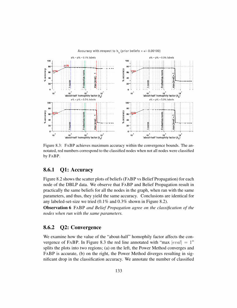
Figure 8.3: FABP achieves maximum accuracy within the convergence bounds. The an-notated, red numbers correspond to the classified nodes when not all nodes were classifiedby FABP.

8.6.1 Q1: AccuracyFigure 8.2 shows the scatter plots of beliefs (FABP vs Belief Propagation) for eachnode of the DBLP data. We observe that FABP and Belief Propagation result inpractically the same beliefs for all the nodes in the graph, when ran with the sameparameters, and thus, they yield the same accuracy. Conclusions are identical forany labeled-set-size we tried (0.1% and 0.3% shown in Figure 8.2).Observation 6 FABP and Belief Propagation agree on the classification of thenodes when run with the same parameters.

8.6.2 Q2: ConvergenceWe examine how the value of the “about-half” homophily factor affects the con-vergence of FABP. In Figure 8.3 the red line annotated with “max |eval| = 1”splits the plots into two regions; (a) on the left, the Power Method converges andFABP is accurate, (b) on the right, the Power Method diverges resulting in sig-nificant drop in the classification accuracy. We annotate the number of classified

133

Figure 8.4: Insensitivity of FABP to themagnitude of the prior beliefs.

Figure 8.5: Running Time of FABP vs #edges for 10 and 30 machines on HADOOP.Kronecker graphs are used.

nodes for the values of hh that leave some nodes unclassified because of numer-ical representation issues. The low accuracy scores for the smallest values of hhare due to the unclassified nodes, which are counted as misclassifications. TheFrobenius norm-based method yields greater upper bound for hh than the 1-normbased method, preventing any numerical representation problems.

Observation 7 Our convergence bounds consistently coincide with high-accuracy regions. Thus, we recommend choosing the homophily factor based onthe Frobenius norm using Equation (8.8).

8.6.3 Q3: Sensitivity to parameters

Figure 8.3 shows that FABP is insensitive to the “about-half” homophily factor,hh, as long as the latter is within the convergence bounds. Moreover, in Figure8.4 we observe that the accuracy score is insensitive to the magnitude of the priorbeliefs. For brevity, we show only the cases a, p ∈ {0.1%, 0.3%, 0.5%}, as for allvalues except for a, p = 5.0%, the accuracy is practical identical. Similar resultswere found for different “about-half” homophily factors, but the plots are omitteddue to lack of space.

Observation 8 The accuracy results are insensitive to the magnitude of the priorbeliefs and homophily factor - as far as the latter is within the convergence boundswe gave in Section 8.4.

134

(a) Runtime vs # of iterations (b) Accuracy vs # iterations (c) Accuracy vs runtime

Figure 8.6: Performance on the YahooWeb graph (best viewed in color): FABP winson speed and wins/ties on accuracy. In (c), each of the method contains 4 points whichcorrespond to the number of steps from 1 to 4. Notice that FABP achieves the maximumaccuracy after 84 minutes, while BP achieves the same accuracy after 151 minutes.

8.6.4 Q4: Scalability

To show the scalability of FABP, we implemented FABP on HADOOP, an opensource MAPREDUCE framework which has been successfully used for large scalegraph analysis [75]. We first show the scalability of FABP on the number of edgesof Kronecker graphs. As seen in Figure 8.5, FABP scales linear on the numberof edges. Next, we compare HADOOP implementation of FABP and BP [71] interms of running time and accuracy on YahooWeb graph. Figures 8.6(a-c) showthat FABP achieves the maximum accuracy level after two iterations of the PowerMethod and is ∼ 2× faster than BP.Observation 9 FABP is linear on the number of edges, with∼ 2× faster runningtime than Belief Propagation on HADOOP.

8.7 Conclusions

Which of the many guilt-by-association methods one should use? We answeredthis question, and we developed FABP, a new, fast algorithm to do such compu-tations. The contributions of our work are the following:• Theory & Correspondences: We showed that successful, major guilt-by-

association approaches (RWR, SSL, and BP variants) are closely related,and we proved that some are even equivalent under certain conditions (The-orem 1, Lemmas 1, 2, 3).

• Algorithms & Convergence: Thanks to our analysis, we designed FABP, afast and accurate approximation to the standard belief propagation (Belief

135

Propagation), which has convergence guarantee (Lemmas 5 and 6).

• Implementation & Experiments: We showed that FABP is significantlyfaster, about 2×, and it has the same or better accuracy (AUC) than BeliefPropagation. Moreover, we show how to parallelize it with MAPREDUCE

(HADOOP), operating on billion-node graphs.Thanks to our analysis, our guide to practitioners is the following: among all 3guilt-by-association methods, we recommend belief propagation, for two reasons:(1) it has solid, Bayesian underpinnings and (2) it can naturally handle heterophily,as well as multiple class-labels. With respect to parameter setting, we recommendto choose homophily score, hh, according to the Frobenius bound (Equation 8.8).

Future work could focus on time-evolving graphs, and label-tracking overtime. For example, in a call-graph, we would like to spot nodes that change be-havior, e.g., from “telemarketer” type to “normal user” type.

136

Chapter 9

OPAvion: Large Graph MiningSystem for Patterns, Anomalies &Visualization

Given a large graph billions of nodes and edges, like a who-follows-whom Twittergraph, how do we scalably compute its statistics, summarize its patterns, spotanomalies, visualize and make sense of it?

A core requirement in accomplishing these tasks is that we need to enable theuser to interact with the data. This chapter presents the OPAVION system thatadopts a hybrid approach that maximizes scalability for algorithms using Hadoop,while enabling interactivity for visualization by using the users local computer asa cache.

OPAVION consists of three modules: (1) The Summarization module(PEGASUS) operates off-line on massive, disk-resident graphs and computesgraph statistics, like PageRank scores, connected components, degree distribu-tion, triangles, etc.; (2) The Anomaly Detection module (ODDBALL) uses graphstatistics to mine patterns and spot anomalies, such as nodes with many contactsbut few interactions with them (possibly telemarketers); (3) The Interactive Visu-alization module (Apolo) lets users incrementally explore the graph, starting withtheir chosen nodes or the flagged anomalous nodes; then users can expand to thenodes’ vicinities, label them into categories, and interactively navigate interestingparts of the graph.

Chapter adapted from work appeared at SIGMOD 2012 [10]

137

9.1 IntroductionWe have entered the era of big data. Massive graphs measured in terabytes oreven petabytes, having billions of nodes and edges, are now common in numerousdomains, such as the link graph of the Web, the friendship graph of Facebook, thecustomer-product graph of Netflix, eBay, etc. How to gain insights into these datais the fundamental challenge. How do we find patterns and anomalies in graphs atsuch massive scale, and how do we visualize them?

Figure 9.1: System overview. OPAVION consists of three modules: the Summarizationmodule (PEGASUS) provides scalable storage and algorithms to compute graph statistics;the Anomaly Detection module (ODDBALL) flags anomalous nodes whose egonet fea-tures deviate from expected distributions; the Visualization module (Apolo) allows theuser to visualize connections among anomalies, expand to their vicinities, label them intocategories, and interactively explore the graph.

We present OPAVION, a system that provides a scalable, interactive workflowto help people accomplish these analysis tasks (see Figure 9.1). Its core capabil-ities and their corresponding modules are:• The Summarization module (PEGASUS) provides massively scalable

graph mining algorithms to compute statistics for the whole graph, such asPageRank, connected components, degree distribution, etc. It also generatesplots that summarize these statistics, to reveal deviations from the expectedgraph’s properties (see Figure 9.3). PEGASUS has been tested to work effi-ciently on a huge graph with 1 billion nodes and 6 billion edges [75].

• The Anomaly Detection module (ODDBALL) automatically detectsanomalous nodes in the graph—for each node, ODDBALL extracts featuresfrom its egonet (induced subgraph formed by the node and its neighbors)and flags nodes whose feature distributions deviate from those of other

138

nodes’. Example features include: number of nodes, total edge weight,principal eigenvalue, etc. These flagged nodes are great points for analysis,as they are potentially new and significant information (see Figure 9.2a forexample anomalies).

• The Visualization module (Apolo) provides an interactive visualizationcanvas for analysts to further their investigation. For example, flaggedanomalous nodes can be transferred to the visualization to show their con-nections (see Figure 9.2b). Different from most graph visualization pack-ages that visualize the full graph, Apolo uses a built-in machine learningmethod called Belief Propagation to guide the user to expand to other rele-vant areas of the graph; the user specifies nodes of interest as exemplars andApolo suggests nodes that are in their close proximity, and their inducedsubgraphs, for further inspection.

Figure 9.2: (a) Illustration of Egonet Density Power Law on the ‘Stack Overflow’ Q&Agraph. Edge count Ei versus node count Ni (log-log scales); red line is the least squaresfit on the median values (dark blue circles) of each bin; dashed black and blue lines haveslopes 1 and 2 respectively, corresponding to stars and cliques. The top anomalies devi-ating from the fit are marked with triangles. (b): Screenshot of the visualization moduleworking with the anomaly detection module, showing a “star” (Sameer, at its center, is ared triangle flagged on the left plot), and a “near-clique” (blue triangles). Nodes are StackOverflow users and a directed edge points from a user who asks a question, to anotheruser who answers it. Node size is proportional to node’s in-degree. Here, user Sameer(the star’s center) is a maven who has answered a lot of questions (high in-degree) fromother users, but he has never interacted with the other mavens in the near-clique who haveboth asked and answered numerous questions.

139

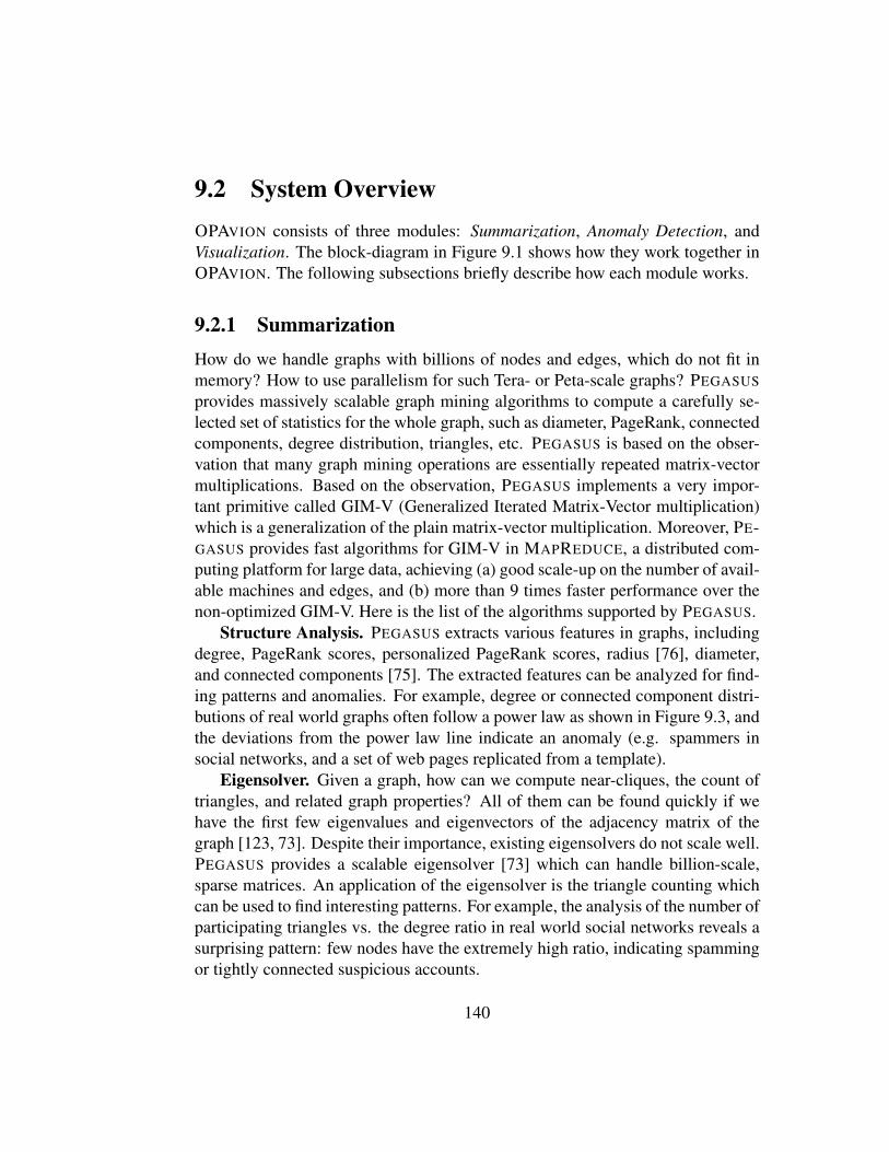
9.2 System OverviewOPAVION consists of three modules: Summarization, Anomaly Detection, andVisualization. The block-diagram in Figure 9.1 shows how they work together inOPAVION. The following subsections briefly describe how each module works.

9.2.1 SummarizationHow do we handle graphs with billions of nodes and edges, which do not fit inmemory? How to use parallelism for such Tera- or Peta-scale graphs? PEGASUS

provides massively scalable graph mining algorithms to compute a carefully se-lected set of statistics for the whole graph, such as diameter, PageRank, connectedcomponents, degree distribution, triangles, etc. PEGASUS is based on the obser-vation that many graph mining operations are essentially repeated matrix-vectormultiplications. Based on the observation, PEGASUS implements a very impor-tant primitive called GIM-V (Generalized Iterated Matrix-Vector multiplication)which is a generalization of the plain matrix-vector multiplication. Moreover, PE-GASUS provides fast algorithms for GIM-V in MAPREDUCE, a distributed com-puting platform for large data, achieving (a) good scale-up on the number of avail-able machines and edges, and (b) more than 9 times faster performance over thenon-optimized GIM-V. Here is the list of the algorithms supported by PEGASUS.

Structure Analysis. PEGASUS extracts various features in graphs, includingdegree, PageRank scores, personalized PageRank scores, radius [76], diameter,and connected components [75]. The extracted features can be analyzed for find-ing patterns and anomalies. For example, degree or connected component distri-butions of real world graphs often follow a power law as shown in Figure 9.3, andthe deviations from the power law line indicate an anomaly (e.g. spammers insocial networks, and a set of web pages replicated from a template).

Eigensolver. Given a graph, how can we compute near-cliques, the count oftriangles, and related graph properties? All of them can be found quickly if wehave the first few eigenvalues and eigenvectors of the adjacency matrix of thegraph [123, 73]. Despite their importance, existing eigensolvers do not scale well.PEGASUS provides a scalable eigensolver [73] which can handle billion-scale,sparse matrices. An application of the eigensolver is the triangle counting whichcan be used to find interesting patterns. For example, the analysis of the number ofparticipating triangles vs. the degree ratio in real world social networks reveals asurprising pattern: few nodes have the extremely high ratio, indicating spammingor tightly connected suspicious accounts.

140

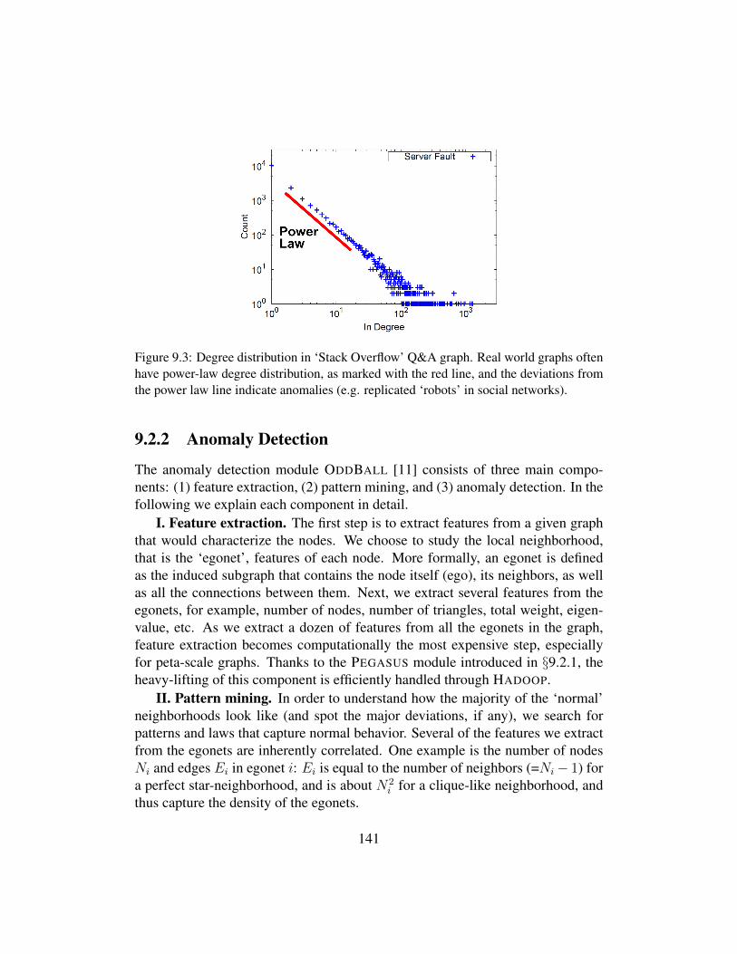
Figure 9.3: Degree distribution in ‘Stack Overflow’ Q&A graph. Real world graphs oftenhave power-law degree distribution, as marked with the red line, and the deviations fromthe power law line indicate anomalies (e.g. replicated ‘robots’ in social networks).

9.2.2 Anomaly Detection

The anomaly detection module ODDBALL [11] consists of three main compo-nents: (1) feature extraction, (2) pattern mining, and (3) anomaly detection. In thefollowing we explain each component in detail.

I. Feature extraction. The first step is to extract features from a given graphthat would characterize the nodes. We choose to study the local neighborhood,that is the ‘egonet’, features of each node. More formally, an egonet is definedas the induced subgraph that contains the node itself (ego), its neighbors, as wellas all the connections between them. Next, we extract several features from theegonets, for example, number of nodes, number of triangles, total weight, eigen-value, etc. As we extract a dozen of features from all the egonets in the graph,feature extraction becomes computationally the most expensive step, especiallyfor peta-scale graphs. Thanks to the PEGASUS module introduced in §9.2.1, theheavy-lifting of this component is efficiently handled through HADOOP.

II. Pattern mining. In order to understand how the majority of the ‘normal’neighborhoods look like (and spot the major deviations, if any), we search forpatterns and laws that capture normal behavior. Several of the features we extractfrom the egonets are inherently correlated. One example is the number of nodesNi and edges Ei in egonet i: Ei is equal to the number of neighbors (=Ni− 1) fora perfect star-neighborhood, and is about N2

i for a clique-like neighborhood, andthus capture the density of the egonets.

141

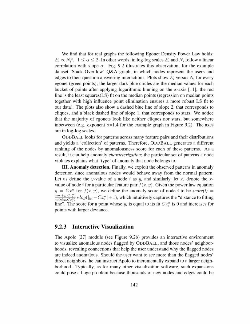
We find that for real graphs the following Egonet Density Power Law holds:Ei ∝ Nα

i , 1 ≤ α ≤ 2. In other words, in log-log scales Ei and Ni follow a linearcorrelation with slope α. Fig. 9.2 illustrates this observation, for the exampledataset ‘Stack Overflow’ Q&A graph, in which nodes represent the users andedges to their question answering interactions. Plots show Ei versus Ni for everyegonet (green points); the larger dark blue circles are the median values for eachbucket of points after applying logarithmic binning on the x-axis [11]; the redline is the least squares(LS) fit on the median points (regression on median pointstogether with high influence point elimination ensures a more robust LS fit toour data). The plots also show a dashed blue line of slope 2, that corresponds tocliques, and a black dashed line of slope 1, that corresponds to stars. We noticethat the majority of egonets look like neither cliques nor stars, but somewhereinbetween (e.g. exponent α=1.4 for the example graph in Figure 9.2). The axesare in log-log scales.

ODDBALL looks for patterns across many feature pairs and their distributionsand yields a ‘collection’ of patterns. Therefore, ODDBALL generates a differentranking of the nodes by anomalousness score for each of these patterns. As aresult, it can help anomaly characterization; the particular set of patterns a nodeviolates explains what ‘type’ of anomaly that node belongs to.

III. Anomaly detection. Finally, we exploit the observed patterns in anomalydetection since anomalous nodes would behave away from the normal pattern.Let us define the y-value of a node i as yi and similarly, let xi denote the x-value of node i for a particular feature pair f(x, y). Given the power law equationy = Cxα for f(x, y), we define the anomaly score of node i to be score(i) =max(yi,Cx

αi )

min(yi,Cxαi )∗ log(|yi−Cxαi |+1), which intuitively captures the “distance to fitting

line”. The score for a point whose yi is equal to its fit Cxαi is 0 and increases forpoints with larger deviance.

9.2.3 Interactive Visualization

The Apolo [27] module (see Figure 9.2b) provides an interactive environmentto visualize anomalous nodes flagged by ODDBALL, and those nodes’ neighbor-hoods, revealing connections that help the user understand why the flagged nodesare indeed anomalous. Should the user want to see more than the flagged nodes’direct neighbors, he can instruct Apolo to incrementally expand to a larger neigh-borhood. Typically, as for many other visualization software, such expansionscould pose a huge problem because thousands of new nodes and edges could be

142

brought up, clouding the screen and overwhelming the user. Instead, Apolo usesits built-in machine learning algorithm called Belief Propagation (BP) to help theuser find the most relevant areas to visualize. The user specifies nodes of interest,such as several flagged nodes as exemplars, and Belief Propagation automaticallyinfers which other nodes may also be of interest to the user. This way, all othernodes can be ranked by their relevance relative to the exemplar nodes, allowingthe user to add only a few of the top-ranking nodes into the visualization.

Belief Propagation is a message passing algorithm over link structure similarto spreading activation, but is uniquely suitable for our visualization purpose, be-cause it simultaneously supports: (1) multiple user-specified exemplars; (2) divid-ing exemplars into any number of groups, which means each node has a relevancescore for each group; and (3) linear scalability with the number of edges, allowingApolo to generate real-time suggestions.

9.3 Example ScenarioHere, we use an example scenario to highlight how OPAVION works. We usethe STACK OVERFLOW Q&A graph (http://stackoverflow.com), whichdescribes over 6 million questions and answers among 650K users. In the graph,nodes are STACK OVERFLOW users, and a directed edge points from the user whoasks a question, to the user who answers it.

In preparation, the Summarization module (PEGASUS) pre-computes thestatistics of the graph (e.g., degree distribution, PageRank scores, radius, con-nected components) and creates plots that show their distributions. Then, theAnomaly Detection module (ODDBALL), using the pre-computed graph statistics,detects anomalous nodes in real time, and shows them in interactive plots (e.g.,Figure 9.2a). The user can mouse-over the flagged nodes, and instruct OPAVION

to show them in the Visualization module (Apolo).In the visualization, users can interact with and navigate the graph, either from

a node they like, or from the flagged anomalies. The user can spatially arrangenodes, and expand their vicinities to reveal surprising connections among theflagged anomalous nodes. For example, Figure 9.2b shows two subgraphs thatinclude nodes flagged in Figure 9.2a (as blue and red triangles): a “star” subgraphwith the user Sameer at its center, and a “near-clique” subgraph (users includeMassimo, Chopper3, etc.). Node size is proportional to the node’s in-degree. Thevisualization reveals that Sameer is a maven who has answered a lot of questions,having a high in-degree, but never asked any questions; on the other hand, the

143

other mavens in the near-clique have a lot of discussion among themselves andnever involve Sameer. It is an great example that shows that two vastly differ-ent anomalous subgraphs—star and near-clique—can actually be very close in thefull graph (in this case, Sameer is only two hops away from the near-clique). Thevisualization helps with this type of discovery.

144

Part IV

Conclusions

145

Chapter 10

Conclusions & Future Directions

We have entered the era of big data. Datasets surpassing terabytes now arise inscience, government and enterprises. Yet, making sense of these data remainsa fundamental challenge. This thesis advocates bridging Data Mining and HCIresearch to help researchers and practitioners to make sense of large graphs withbillions of nodes and edges.

10.1 Contributions

We contributes by answering important, fundamental research questions in bigdata analytics, such as:

• Where to start our analysis? Part I presents the attention routing ideabased on anomaly detection and machine inference that automatically drawspeople’s attention to interesting parts of the graph, instead of doing thatmanually. We describe several examples. Polonium unearths malware from37 billion machine-file relationships (Chapter 4). NetProbe fingers bad guyswho commit auction fraud (Chapter 3).

• Where to go next? Part II presents examples that combine techniques fromdata mining, machine learning and interactive visualization to help userslocate the next areas of interest. Apolo (Chapter 5) guides the user to inter-actively explore large graphs by learning from few examples given by theuser. Graphite (Chapter 6) finds potentially interesting regions of the entiregraph, based on only fuzzy descriptions from the user drawn graphically.

• How to scale up? Part III presents examples of scaling up our methods to

147

web-scale, billion-node graphs, by leveraging Hadoop (Chapter 7), approx-imate computation (Chapter 8), and staging of operations (Chapter 9).

We contribute to data mining, HCI, and importantly at their intersection:• Algorithms & Systems: we contribute a cohesive collection of algorithms

that scale to massive networks such as Belief Propagation on Hadoop(Chapter 7, 8), and we are making them publicly available to the researchcommunity as the Pegasus project (http://www.cs.cmu.edu/˜pegasus).Our other scalable systems include: OPAvion for scalable mining and vi-sualization (Chapter 9); Apolo for exploring large graph (Chapter 5); andGraphite for matching user-specified subgraph patterns (Chapter 6).

• Theories: We present theories that unify graph mining approaches (e.g.,Chapter 8), which enable us to make algorithms even more scalable.

• Applications: Inspired by graph mining research, we formulate and solveimportant real-world problems with ideas, solutions, and implementationsthat are first of their kinds. We tackled problems such as detecting auctionfraudsters (Chapter 3) and unearthing malware (Chapter 4).

• New Class of InfoVis Methods: Our Attention Routing idea (Part I) addsa new class of nontrivial methods to information visualization, as a viableresource for the critical first step of locating starting points for analysis.

• New Analytics Paradigm: Apolo (Chapter 5) represents a paradigm shiftin interactive graph analytics. The conventional paradigm in visual analyticsrelies on first generating a visual overview for the entire graph which is notpossible for most massive, real-world graphs. Here, Apolo enables users toevolve their mental models of the graph in a bottom-up manner, by startingsmall, rather starting big and drilling down.

• Scalable Interactive Tools: Our interactive tools (e.g., Apolo, Graphite)advances the state of the art, by enabling people to interact with graphsorders of magnitudes larger in real time (tens of millions of edges).

This thesis research opens up opportunities for a new breed of systems andmethods that combine HCI and data mining methods to enable scalable, interac-tive analysis of big data. We hope that our thesis, and our big data mantra “Ma-chine for Attention Routing, Human for Interaction” will serve as the catalyst thataccelerates innovation across these disciplines, and the bridge that connects them.inspiring more researchers and practitioners to work together at the crossroad ofData Dining and HCI.

148

10.2 ImpactThis thesis work has made remarkable impact to the research community andsociety at large:• Polonium (Chapter 4), part of Symantec’s flagship Norton Antivirus prod-

ucts, protects 120 million people worldwide from malware (also patent-pending), and has answered over trillions of queries for file reputationqueries. Polonium is patent-pending.

• NetProbe (Chapter 3) fingers fraudsters on eBay, made headlines in majormedia outlets, like Wall Street Journal, CNN, and USA Today. Interestedby our work, eBay invited us for a site visit and presentation.

• Pegasus (Chapter 7 & 9), which creates scalable graph algorithms, won theOpen Source Software World Challenge, Silver Award. We have releasedPegasus as free, open-source software, downloaded by people from over 83countries. It is also part of Windows Azure, Microsoft’s cloud computingplatform.

• Apolo (Chapter 5) contributes to DARPA’s Anomaly Detection at MultipleScales project (ADAMS) to detect insider threats and prevent exfiltration ingovernment and the military.

10.3 Future Research DirectionsThis thesis takes a major step in bridging the fields of data mining and HCI, totap into their complementing connections, to develop tools that combine the bestof both worlds–enabling humans to best use their perceptual abilities and intuitionto drill down in data, and leveraging computers to sift through huge data to sportpatterns and anomalies.

For the road ahead, I hope to broaden and deepen this investigation, extendingmy work to more domains and applications, such as bioinfomatics, law enforce-ment, national security, and intelligence analysis. Initially, I will focus on thefollowing three interrelated research directions.

Generalizing to More Data Types My hybrid approach of combining data min-ing and HCI methods applies to not only graph data, but also to other importantdata types, such as time series and unstructured data, like text documents. Alongthis direction, I have started developing the TopicViz system [45] for making sense

149

of large document collections, by using topic modeling (Latent Dirichlet alloca-tion) to identify document themes, and providing a direct-manipulation interfacefor the user to explore them.

Collaborative Analysis of Big Data Most analytics systems today are designedfor a single user. As datasets become more complex, they will require multiple an-alysts to work together, possibly remotely, to combine their efforts and expertise.I plan to study how to support such collaborative analysis on massive datasets, de-sign visualizations that intuitively communicate analysts’ progress and findings toeach other, and develop machine learning methods that aggregate analysts’ feed-back for collective inference.

Interactive Analytics Platform of the Future My research harnesses the par-allelism of the Hadoop platform [71, 10] to scale up computation power and stor-age. However, interactive analytics requires real-time access to the computationresults. I plan to enable this in two research directions: (1) explore technologiessuch as HBase (modeled after Google’s Bigtable) to provide real-time access tothe big data; (2) decouple algorithms into complimentary online and offline parts,such that a large part of the computation can be pre-computed, then queried andcombined with fast, online computation whenever the user issues a command. Iam interested in developing new platforms that balance scalability with timeliness,for computation, interaction and visualization.

150

Appendix A

Analysis of FABP in Chapter 8

A.1 PreliminariesWe give the lemmas needed to prove Theorem 1 (FABP) in Section 8.3. We startwith the original BP equations, and we derive the proof by:• using the odds ratio pr = p/(1−p), instead of probabilities. The advantage

is that we have only one value for each node (pr(i), instead of two: p+(i),p−(i)) and, also, the normalization factor is not needed. Moreover, workingwith the odds ratios results in the substitution of the propagation matrixentries by a scalar homophily factor.

• assuming that all the parameters are close to 1/2, using MacLaurin expan-sions to linearize the equations, and keeping only the first order terms. Bydoing so we avoid the sigmoid/non-linear equations of BP.

Traditional BP equations In [155], Yedidia derives the following update for-mulas for the messages sent from node i to node j and the belief of each node thatit is in state xi

mij(xj) =∑xi

φi(xi) · ψij(xi, xj) ·∏

n∈N(i)\j

mni(xi) (A.1)

bi(xi) = η · φi(xi) ·∏

j∈N(i)

mij(xi) (A.2)

where the message from node i to node j is computed based on all the messagessent by all its neighbors in the previous step except for the previous message sent

151

Table A.1: Additional Symbols and Definitions

Symbols Definitionsp P(node in positive class) = P(“+”)m message

< var >r odds ratio = <var>1−<var> , where < var >= b, φ, m, h

B(a, b) blending function = a·b+1a+b

.

from node j to node i. N(i) denotes the neighbors of i and η is a normalizationconstant that guarantees that the beliefs sum to 1.Lemma 3 Expressed as ratios, the BP equations become:

mr(i, j)← B[hr, br,adjusted(i, j)] (A.3)

br(i)← φr(i) ·∏

j∈N(i)

mr(j, i) (A.4)

where br,adjusted(i, j) is defined as br,adjusted(i, j) = br(i)/mr(j, i). The divisionby mr(j, i) subtracts the influence of node j when preparing the message m(i, j).Proof 9 The proof is straightforward; we omit it due to lack of space. QEDLemma 4 (Approximations) Fundamental approximations for all the variablesv, a, b of interest, {m, b, φ, h}, that we use for the rest of our lemmas:

vr =v

1− v=

1/2 + vh1/2− vh

≈ 1 + 4vh (A.5)

B(ar, br) ≈ 1 + 8ahbh (A.6)

where B(ar, br) is the blending function for any variables ar, br.Proof 10 (Sketch of proof) Use the definition of “about-half” approximations,apply the appropriate MacLaurin series expansions and keep only the first orderterms. QEDThe following 3 lemmas are useful in order to derive the linear equation of FABP.Note that in all the lemmas we apply several approximations in order to linearizethe equations; we omit the “≈” symbol so that the proofs are more readable.Lemma 7 The about-half version of the belief equation becomes, for small devi-ations from the half-point:

bh(i) ≈ φh(i) +∑j∈N(i)

mh(j, i). (A.7)

152

Proof 11 We use the Equations (A.4) and (A.5) and apply the appropriateMacLaurin series expansions:

br(i) = φr(i)∏

j∈N(i)

mr(j, i)⇒

log (1 + 4bh(i)) = log (1 + 4φh(i)) +∑jεN(i)

log (1 + 4mh(j, i))⇒

bh(i) = φh(i) +∑jεN(i)

mh(j, i).

QED

Lemma 8 The about-half version of the message equation becomes:

mh(i, j) ≈ 2hh[bh(i)−mh(j, i)]. (A.8)

Proof 12 We combine the Equations (A.3), (A.5) and (A.6)

mr(i, j) = B[hr, br,adjusted(i, j)]⇒ mh(i, j) = 2hhbh,adjusted(i, j). (A.9)

In order to derive bh,adjusted(i, j) we use Equation (A.5) and the approximation ofthe MacLaurin expansion 1

1+ε= 1− ε for a small quantity ε:

br,adjusted(i, j) = br(i)/mr(j, i)⇒1 + bh,adjusted(i, j) = (1 + 4bh(i))(1− 4mh(j, i))⇒

bh,adjusted(i, j) = bh(i)−mh(j, i)− 4bh(i)mh(j, i) . (A.10)

Substituting Equation (A.10) to Equation (A.9) and ignoring the terms of secondorder leads to the about-half version of the message equation. QED

Lemma 9 At steady state, the messages can be expressed in terms of the beliefs:

mh(i, j) ≈2hh

(1− 4h2h)[bh(i)− 2hhbh(j)] (A.11)

Proof 13 We apply Lemma 8 both for mh(i, j) and mh(j, i) and we solve formh(i, j). QED

153

A.2 Proofs of TheoremsHere we give the proofs of the theorems and lemmas presented in Section 8.3.Proof of Theorem 1. We substitute Equation (A.8) to Equation (A.7) and we ob-tain:

bh(i)−∑j∈N(i)

mh(j, i) = φh(i)⇒

bh(i) +∑j∈N(i)

4h2hbh(j)

1− 4h2h−∑j∈N(i)

2hh1− 4h2h

bh(i) = φh(i)⇒

bh(i) + α∑j∈N(i)

bh(i)− c′∑j∈N(i)

bh(j) = φh(i)⇒

(I + aD− c′A)bh = φh .

QEDopen

Proof of Lemma 2. Given l labeled points (xi, yi), i = 1, . . . , l, and u unlabeledpoints xl+1, . . . , xl+u for a semi-supervised learning problem, based on an energyminimization formulation, we solve the labels xi by minimizing the followingfunctional E

E(x) = α∑j∈N(i)

aij(xi − xj)2 +∑1≤i≤l

(yi − xi)2 , (A.12)

where α is related to the coupling strength (homophily), of neighboring nodes.N(i) denotes the neighbors of i. If all points are labeled, in matrix form, thefunctional can be re-written as

E(x) = xT [I + α(D−A)]x− 2x · y +K(y)

= (x− x∗)T [I + α(D−A)](x− x∗) +K ′(y) ,

where x∗ = [I+α(D−A)]−1y, andK,K ′ are some constant terms which dependonly on y. Clearly, E achieves the minimum when

x = x∗ = [I + α(D−A)]−1y

The equivalence of SSL and Gaussian BP can be found in [151]. QED

154

Proof of Lemma 3. Based on Equations (8.2) and (8.3), the two methods willgive identical results if

(1− c)[I− cD−1A]−1 = [I + α(D−A)]−1 ⇔

(1

(1− c)I− c

(1− c)D−1A)−1 = (α(D−A) + I)−1 ⇔(

1

1− c

)I−

(c

1− c

)D−1A = I + α(D−A)⇔(

c

1− c

)I−

(c

1− c

)D−1A = α(D−A)⇔(

c

1− c

)[I−D−1A] = α(D−A)⇔(

c

1− c

)D−1[D−A] = α(D−A)⇔(c

1− c

)D−1 = αI .

This cannot hold in general, unless the graph is “regular”: di = d (i = 1, . . .), orD = d · I, in which case the condition becomes

α =c

(1− c)d⇒ c =

αd

1 + αd(A.13)

where d is the common degree of all the nodes. QED

A.3 Proofs for ConvergenceProof of Lemma 5. In order for the power series to converge, a sub-multiplicative norm of matrix W = cA − aD should be smaller than 1. In thisanalysis we use the 1-norm (or equivalently the∞-norm). The elements of matrixW are either c = 2hh

1−4h2hor −adii =

−4h2hdii1−4h2h

. Thus, we require

maxj

(n∑i=1

|Aij|) < 1⇒ (c+ a) ·maxjdjj < 1

2h

1− 2hmaxjdjj < 1⇒ hh <

1

2(1 + maxj djj).

QED

155

156

Bibliography

[1] Graphviz. http://www.graphviz.org/.

[2] Hadoop information. http://hadoop.apache.org/.

[3] Jung. http://jung.sourceforge.net/.

[4] Otter. http://warriors.eecs.umich.edu/viz tools/otter.html.

[5] Prefuse. http://prefuse.org/.

[6] Walrus. http://www.caida.org/tools/visualization/walrus/.

[7] J. Abello, F. Van Ham, and N. Krishnan. Ask-graphview: A large scalegraph visualization system. IEEE Transactions on Visualization and Com-puter Graphics, pages 669–676, 2006.

[8] E. Adar. Guess: a language and interface for graph exploration. In Proc.CHI, page 800. ACM, 2006.

[9] C. C. Aggarwal and P. S. Yu. Outlier detection for high dimensional data.In SIGMOD, pages 37–46, 2001.

[10] L. Akoglu, D. Chau, U. Kang, D. Koutra, and C. Faloutsos. Opavion:Mining and visualization in large graphs. SIGMOD, 2012.

[11] L. Akoglu, M. McGlohon, and C. Faloutsos. Oddball: Spotting anomaliesin weighted graphs. In PAKDD, 2010.

[12] B. Amento, W. Hill, L. Terveen, D. Hix, and P. Ju. An empirical evaluationof user interfaces for topic management of web sites. In Proc. CHI, page559. ACM, 1999.

[13] J. Anderson. A spreading activation theory of memory. Journal of verballearning and verbal behavior, 22(3):261–95, 1983.

[14] A. Arning, R. Agrawal, and P. Raghavan. A linear method for deviationdetection in large databases. In KDD, pages 164–169, 1996.

157

[15] Auctionbytes: ebay auction fraud spawns vigilantism trend. http://www.auctionbytes.com/cab/abn/y02/m10/i12/s01, 2002.

[16] M. Q. W. Baldonado and T. Winograd. Sensemaker: an information-exploration interface supporting the contextual evolution of a user’s inter-ests. In Proc. CHI, pages 11–18. ACM Press New York, NY, USA, 1997.

[17] V. Barnett and T. Lewis. Outliers in Statistical Data. John Wiley and Sons,Chichester, New York, 1994.

[18] L. Barsalou. Ad hoc categories. Memory & Cognition, 11(3):211–227,May 1983.

[19] R. Behrman and K. Carley. Modeling the structure and effectiveness ofintelligence organizations: Dynamic information flow simulation. In Pro-ceedings of the 8th International Command and Control Research andTechnology Symposium., 2003.

[20] G. Bhalotia, A. Hulgeri, C. Nakhe, S. Chakrabarti, and S. Sudarshan. Key-word searching and browsing in databases using banks. In ICDE ’02: Pro-ceedings of the 18th International Conference on Data Engineering, pages431–440, 2002.

[21] M. M. Breunig, H.-P. Kriegel, R. T. Ng, and J. Sander. Lof: Identifyingdensity-based local outliers. In SIGMOD, pages 93–104, 2000.

[22] S. Brin and L. Page. The anatomy of a large-scale hypertextual Web searchengine. Computer networks and ISDN systems, 30(1-7):107–117, 1998.

[23] S. Card, G. Robertson, and W. York. The WebBook and the Web Forager:an information workspace for the World-Wide Web. In Proc. CHI. ACM,1996.

[24] R. Chaiken, B. Jenkins, P.-A. Larson, B. Ramsey, D. Shakib, S. Weaver,and J. Zhou. Scope: easy and efficient parallel processing of massive datasets. VLDB, 2008.

[25] D. Chakrabarti. Autopart: Parameter-free graph partitioning and outlierdetection. In PKDD, pages 112–124, 2004.

[26] D. Chakrabarti, S. Papadimitriou, D. S. Modha, and C. Faloutsos. Fullyautomatic cross-associations. In KDD Conference, pages 79–88, Seattle,WA, 2004.

[27] D. Chau, A. Kittur, J. I. Hong, and F. C. Apolo: Making Sense of LargeNetwork Data by Combining Rich User Interaction and Machine Learning.

158

In Proceeding of the twenty-ninth annual SIGCHI conference on Humanfactors in computing systems. ACM, 2011.

[28] D. Chau, C. Nachenberg, J. Wilhelm, A. Wright, and C. Faloutsos. Polo-nium: Tera-scale graph mining and inference for malware detection. SIAMInternational Conference on Data Mining, 2011.

[29] D. H. Chau and C. Faloutsos. Fraud detection in electronic auction. InEuropean Web Mining Forum at ECML/PKDD, 2005.

[30] D. H. Chau, C. Faloutsos, H. Tong, J. I. Hong, B. Gallagher, and T. Eliassi-Rad. Graphite: A visual query system for large graphs. In ICDM Work-shops, pages 963–966, 2008.

[31] D. H. Chau, S. Pandit, and C. Faloutsos. Detecting fraudulent personalitiesin networks of online auctioneers. In Proc. ECML/PKDD, 2006.

[32] A. Chaudhary, A. S. Szalay, and A. W. Moore. Very fast outlier detectionin large multidimensional data sets. In DMKD, 2002.

[33] A. Chechetka and C. Guestrin. Focused belief propagation for query-specific inference. In International Conference on Artificial Intelligenceand Statistics (AISTATS), May 2010.

[34] N. A. Christakis and J. H. Fowler. The spread of obesity in a large socialnetwork over 32 years. New England Journal of Medicine, 357(4):370–379,2007.

[35] M. Christodorescu, S. Jha, and C. Kruegel. Mining specifications of mali-cious behavior. In Proceedings of the the 6th joint meeting of the Europeansoftware engineering conference and the ACM SIGSOFT symposium onThe foundations of software engineering, pages 5–14. ACM, 2007.

[36] M. Christodorescu, S. Jha, S. Seshia, D. Song, and R. Bryant. Semantics-Aware Malware Detection. In Proceedings of the 2005 IEEE Symposiumon Security and Privacy, page 46. IEEE Computer Society, 2005.

[37] C. Chua and J. Wareham. Fighting internet auction fraud: An assessmentand proposal. In Computer, volume 37 no. 10, pages 31–37, 2004.

[38] D. Cutting, D. Karger, J. Pedersen, and J. Tukey. Scatter/gather: A cluster-based approach to browsing large document collections. In Proc. SIGIR,pages 318–329. ACM Press, 1992.

[39] J. Dean and S. Ghemawat. Mapreduce: Simplified data processing on largeclusters. OSDI, 2004.

159

[40] B. Dervin. An overview of sense-making research: concepts, methods andresults to date. In International Communications Association Annual Meet-ing, 1983.

[41] G. Di Battista, P. Eades, R. Tamassia, and I. Tollis. Graph drawing: al-gorithms for the visualization of graphs. Prentice Hall PTR Upper SaddleRiver, NJ, USA, 1998.

[42] ebay inc. announces third quarter 2006 financial results. http://biz.yahoo.com/bw/061018/20061018005916.html?.v=1, Octo-ber 2006.

[43] ebay: Avoiding fraud. http://pages.ebay.com/securitycenter/avoiding_fraud.html, 2006.

[44] W. Eberle and L. B. Holder. Discovering structural anomalies in graph-based data. In ICDM Workshops, pages 393–398, 2007.

[45] J. Eisenstein, D. Chau, A. Kittur, and E. Xing. Topicviz: interactive topicexploration in document collections. In Proceedings of the 2012 ACM an-nual conference extended abstracts on Human Factors in Computing Sys-tems Extended Abstracts, pages 2177–2182. ACM, 2012.

[46] C. Faloutsos, K. S. McCurley, and A. Tomkins. Fast discovery of con-nection subgraphs. In KDD ’04: Proceedings of the 10th ACM SIGKDDInternational Conference on Knowledge Discovery and Data Mining, page118127, 2004.

[47] P. Felzenszwalb and D. Huttenlocher. Efficient belief propagation for earlyvision. International journal of computer vision, 70(1):41–54, 2006.

[48] J. H. Fowler and N. A. Christakis. Dynamic spread of happiness in a largesocial network: longitudinal analysis over 20 years in the FraminghamHeart Study. BMJ, 2008.

[49] Federal trade commission: Internet auctions: A guide for buyers andsellers. http://www.ftc.gov/bcp/conline/pubs/online/auctions.htm, 2004.

[50] B. Gallagher. Matching structure and semantics: A survey on graph-basedpattern matching. In AAAI FS ’06: Papers from the 2006 AAAI Fall Sym-posium on Capturing and Using Patterns for Evidence Detection, pages45–53, 2006.

[51] J. Gao, F. Liang, W. Fan, Y. Sun, and J. Han. Graph-based Consensus

160

Maximization among Multiple Supervised and Unsupervised Models. InNIPS, 2009.

[52] J. Gonzalez, Y. Low, and C. Guestrin. Residual splash for optimally paral-lelizing belief propagation. AISTATS, 2009.

[53] J. Gonzalez, Y. Low, C. Guestrin, and D. O’Hallaron. Distributed parallelinference on large factor graphs. In Conference on Uncertainty in ArtificialIntelligence (UAI), Montreal, Canada, July 2009.

[54] R. L. Grossman and Y. Gu. Data mining using high performance dataclouds: experimental studies using sector and sphere. KDD, 2008.

[55] S. Guha, R. Rastogi, and K. Shim. Cure: An efficient clustering algorithmfor large databases. Inf. Syst., 26(1):35–58, 2001.

[56] Z. Gyongyi, H. Garcia-Molina, and J. Pedersen. Combating web spam withtrustrank. In VLDB ‘04, page 587. VLDB Endowment, 2004.

[57] T. Haveliwala. Topic-sensitive pagerank: A context-sensitive ranking algo-rithm for web search. IEEE transactions on knowledge and data engineer-ing, pages 784–796, 2003.

[58] T. Haveliwala, S. Kamvar, and G. Jeh. An analytical comparison of ap-proaches to personalizing pagerank. Technical report, Stanford University,2003.

[59] D. Hawkins. Identification of outliers. Chapman and Hall, 1980.

[60] J. Heer and D. Boyd. Vizster: Visualizing online social networks. Proc.InfoVis, pages 33–40, 2005.

[61] J. Heer, S. K. Card, and J. A. Landay. prefuse: a toolkit for interactiveinformation visualization. In Proc. CHI, pages 421–430, New York, NY,USA, 2005. ACM.

[62] I. Herman, G. Melancon, and M. S. Marshall. Graph visualization andnavigation in information visualization: A survey. IEEE Transactions onVisualization and Computer Graphics, 6(1):24–43, 2000.

[63] K. Holyoak and P. Thagard. Mental leaps: Analogy in creative thought.The MIT Press, 1996.

[64] N. Idika and A. P. Mathur. A Survey of Malware Detection Techniques.Technical report, Department of Computer Science, Purdue University,2007.

[65] Internet fraud complaint center: Ic3 2004 internet fraud - crime

161

report. http://www.ifccfbi.gov/strategy/statistics.asp, 2005.

[66] M. Ji, Y. Sun, M. Danilevsky, J. Han, and J. Gao. Graph regularizedtransductive classification on heterogeneous information networks. ECMLPKDD’10, 2010.

[67] R. Jin, C. Wang, D. Polshakov, S. Parthasarathy, and G. Agrawal. Discover-ing frequent topological structures from graph datasets. In KDD ’05: Pro-ceedings of the 11th ACM SIGKDD International Conference on Knowl-edge Discovery and Data Mining, pages 606–611, 2005.

[68] R. A. Johnson and D. W. Wichern. Applied Multivariate Statistical Analy-sis. Prentice Hall, 1998.

[69] Y. Kammerer, R. Nairn, P. Pirolli, and E. H. Chi. Signpost from the masses:learning effects in an exploratory social tag search browser. In Proc. CHI,2009.

[70] U. Kang, D. Chau, and C. Faloutsos. Inference of beliefs on billion-scalegraphs. The 2nd Workshop on Large-scale Data Mining: Theory and Ap-plications, 2010.

[71] U. Kang, D. H. Chau, and C. Faloutsos. Mining large graphs: Algorithms,inference, and discoveries. In ICDE, pages 243–254, 2011.

[72] U. Kang, M. McGlohon, L. Akoglu, and C. Faloutsos. Patterns on theconnected components of terabyte-scale graphs. IEEE International Con-ference on Data Mining, 2010.

[73] U. Kang, B. Meeder, and C. Faloutsos. Spectral analysis for billion-scalegraphs: Discoveries and implementation. In PAKDD (2), pages 13–25,2011.

[74] U. Kang, C. Tsourakakis, A. P. Appel, C. Faloutsos, and J. Leskovec. Ra-dius plots for mining tera-byte scale graphs: Algorithms, patterns, and ob-servations. SIAM International Conference on Data Mining, 2010.

[75] U. Kang, C. Tsourakakis, and C. Faloutsos. PEGASUS: A peta-scale graphmining system implementation and observations. In Data Mining, 2009.ICDM’09. Ninth IEEE International Conference on, pages 229–238. IEEE,2009.

[76] U. Kang, C. E. Tsourakakis, A. P. Appel, C. Faloutsos, and J. Leskovec.Hadi: Mining radii of large graphs. ACM Trans. Knowl. Discov. Data,

162

5:8:1–8:24, February 2011.

[77] G. Karypis and V. Kumar. METIS: Unstructured graph partitioning andsparse matrix ordering system. The University of Minnesota, 2.

[78] L. Kaufman and P. J. Rousseeuw. Finding Groups in Data: An Introductionto Cluster Analysis. John Wiley, 1990.

[79] F. Keil. Concepts, kinds, and cognitive development. The MIT Press, 1989.

[80] J. Kephart and W. Arnold. Automatic extraction of computer virus sig-natures. In 4th Virus Bulletin International Conference, pages 178–184,1994.

[81] J. Kleinberg. Authoritative sources in a hyperlinked environment. In Proc.9th ACM-SIAM Symposium on Discrete Algorithms, 1998.

[82] P. Klerks. The network paradigm applied to criminal organisations. Con-nections, 24(3):53–65, 2001.

[83] E. M. Knorr and R. T. Ng. Algorithms for mining distance-based outliersin large datasets. In VLDB, pages 392–403, 1998.

[84] J. Kolter and M. Maloof. Learning to detect and classify malicious exe-cutables in the wild. The Journal of Machine Learning Research, 7:2744,2006.

[85] Y. Koren, S. C. North, and C. Volinsky. Measuring and extracting proximityin networks. In KDD, pages 245–255. ACM, 2006.

[86] D. Koutra, T. Ke, U. Kang, D. Chau, H. Pao, and C. Faloutsos. Unifyingguilt-by-association approaches: Theorems and fast algorithms. MachineLearning and Knowledge Discovery in Databases, pages 245–260, 2011.

[87] B. Kules, M. Wilson, M. Schraefel, and B. Shneiderman. From keywordsearch to exploration: How result visualization aids discovery on the web.Human-Computer Interaction Lab Technical Report HCIL-2008-06, Uni-versity of Maryland, pages 2008–06, 2008.

[88] V. Kwatra, A. Schodl, I. Essa, G. Turk, and A. Bobick. Graphcut textures:Image and video synthesis using graph cuts. ACM Transactions on Graph-ics, 22(3):277–286, 2003.

[89] R. Lammel. Google’s mapreduce programming model – revisited. Scienceof Computer Programming, 70:1–30, 2008.

[90] B. Lee, C. Parr, C. Plaisant, B. Bederson, V. Veksler, W. Gray, and C. Kot-fila. Treeplus: Interactive exploration of networks with enhanced tree lay-

163

outs. TVCG, pages 1414–1426, 2006.

[91] J. Leskovec, D. Chakrabarti, J. M. Kleinberg, and C. Faloutsos. Realistic,mathematically tractable graph generation and evolution, using kroneckermultiplication. PKDD, pages 133–145, 2005.

[92] J. Leskovec and C. Faloutsos. Sampling from large graphs. KDD, pages631–636, 2006.

[93] Y. Maarek, M. Jacovi, M. Shtalhaim, S. Ur, D. Zernik, and I. Ben-Shaul.WebCutter: a system for dynamic and tailorable site mapping. ComputerNetworks and ISDN Systems, 29(8-13):1269–1279, 1997.

[94] J. Mackinlay, R. Rao, and S. Card. An organic user interface for searchingcitation links. In Proc. CHI, page 73. ACM, 1995.

[95] S. A. Macskassy and F. Provost. Suspicion scoring based on guilt-by-association, collective inference, and focused data access. In Proceedingsof the NAACSOS Conference, June 2005.

[96] D. M. Malioutov, J. K. Johnson, and A. S. Willsky. Walk-sums and beliefpropagation in gaussian graphical models. Journal of Machine LearningResearch, 7:2031–2064, 2006.

[97] M. Mcglohon, L. Akoglu, and C. Faloutsos. Weighted graphs and dis-connected components: Patterns and a generator. In ACM Special Inter-est Group on Knowledge Discovery and Data Mining (SIG-KDD), August2008.

[98] M. McGlohon, S. Bay, M. Anderle, D. Steier, and C. Faloutsos. SNARE: alink analytic system for graph labeling and risk detection. In SIGKDD ‘09,pages 1265–1274. ACM New York, NY, USA, 2009.

[99] G. McKiernan. New Age Navigation. The Serials Librarian, 45(2):87–123,2003.

[100] M. Melnik and J. Alm. Does a seller’s ecommerce reputation matter? ev-idence from ebay auctions. Journal of Industrial Economics, 50:337–49,2002.

[101] A. Mendiburu, R. Santana, J. Lozano, and E. Bengoetxea. A parallel frame-work for loopy belief propagation. GECCO, 2007.

[102] G. Miller. The magical number seven, plus or minus two: some limits onour capacity for processing information. Psychological review, 63(2):81,1956.

164

[103] E. Minkov and W. Cohen. Learning to rank typed graph walks: Local andglobal approaches. In Proceedings of the 9th WebKDD and 1st SNA-KDD2007 workshop on Web mining and social network analysis, pages 1–8.ACM, 2007.

[104] K. Misue, P. Eades, W. Lai, and K. Sugiyama. Layout adjustment and themental map. Journal of Visual Languages and Computing, 6(2):183–210,1995.

[105] B. Myers, S. Hudson, and R. Pausch. Past, present, and future of userinterface software tools. TOCHI, 7(1):3–28, 2000.

[106] J. Neville and D. Jensen. Collective Classification with Relational Depen-dency Networks. In Workshop on Multi-Relational Data Mining (MRDM-2003), page 77.

[107] O. Neville, J. and simsek, D. Jensen, J. Komoroske, K. Palmer, andH. Goldberg. Using relational knowledge discovery to prevent securitiesfraud. In SIGKDD ‘05, page 458. ACM, 2005.

[108] A. Ng, M. Jordan, and Y. Weiss. On spectral clustering: Analysis andan algorithm. In Advances in Neural Information Processing Systems 14:Proceeding of the 2001 Conference, pages 849–856, 2001.

[109] R. T. Ng and J. Han. Efficient and effective clustering methods for spatialdata mining. In VLDB, pages 144–155, 1994.

[110] C. C. Noble and D. J. Cook. Graph-based anomaly detection. In KDD,pages 631–636, 2003.

[111] C. Olston, B. Reed, U. Srivastava, R. Kumar, and A. Tomkins. Pig latin: anot-so-foreign language for data processing. In SIGMOD ’08, pages 1099–1110, 2008.

[112] J. OMadadhain, D. Fisher, P. Smyth, S. White, and Y. Boey. Analysis andvisualization of network data using JUNG. Journal of Statistical Software,10:1–35, 2005.

[113] J. Pan, H. Yang, C. Faloutsos, and P. Duygulu. Gcap: Graph-based auto-matic image captioning. 2004.

[114] S. Pandit, D. Chau, S. Wang, and C. Faloutsos. Netprobe: a fast and scal-able system for fraud detection in online auction networks. In Proceedingsof the 16th international conference on World Wide Web, pages 201–210.ACM, 2007.

165

[115] S. Papadimitriou, H. Kitagawa, P. B. Gibbons, and C. Faloutsos. Loci: Fastoutlier detection using the local correlation integral. In ICDE, pages 315–,2003.

[116] S. Papadimitriou and J. Sun. Disco: Distributed co-clustering with map-reduce. ICDM, 2008.

[117] J. Pearl. Reverend Bayes on inference engines: A distributed hierarchicalapproach. In Proceedings of the AAAI National Conference on AI, pages133–136, 1982.

[118] J. Pearl. Probabilistic reasoning in intelligent systems: networks of plausi-ble inference. Morgan Kaufmann, 1988.

[119] J. Pei, D. Jiang, and A. Zhang. On mining cross-graph quasi-cliques. InSIGKDD ‘05, page 238. ACM, 2005.

[120] A. Perer and B. Shneiderman. Integrating statistics and visualization: casestudies of gaining clarity during exploratory data analysis. In Proc. CHI,pages 265–274, New York, NY, USA, 2008. ACM.

[121] R. Pike, S. Dorward, R. Griesemer, and S. Quinlan. Interpreting the data:Parallel analysis with sawzall. Scientific Programming Journal, 2005.

[122] P. Pirolli and S. Card. The sensemaking process and leverage points foranalyst technology as identified through cognitive task analysis. In Proc.IA, 2005.

[123] B. A. Prakash, M. Seshadri, A. Sridharan, S. Machiraju, and C. Faloutsos.Eigenspokes: Surprising patterns and community structure in large graphs.PAKDD, 2010.

[124] P. Resnick, R. Zeckhauser, E. Friedman, and K. Kuwabara. Reputationsystems. Communications of the ACM, 43, 2000.

[125] P. Resnick, R. Zeckhauser, J. Swanson, and K. Lockwood. The value ofreputation on ebay: A controlled experiment, 2003.

[126] E. Rosch and C. Mervis. Family resemblances: Studies in the internalstructure of categories. Cognitive psychology, 7(4):573–605, 1975.

[127] D. M. Russell, M. Slaney, Y. Qu, and M. Houston. Being literate with largedocument collections: Observational studies and cost structure tradeoffs.In HICSS, page 55. IEEE, 2006.

[128] D. M. Russell, M. J. Stefik, P. Pirolli, and S. K. Card. The cost structure ofsensemaking. In Proc. CHI, pages 269–276. ACM Press, 1993.

166

[129] K. Ryall, J. Marks, and S. Shieber. An interactive constraint-based systemfor drawing graphs. In Proc. UIST, pages 97–104. ACM, 1997.

[130] M. Schultz, E. Eskin, E. Zadok, and S. Stolfo. Data mining methods fordetection of new malicious executables. In IEEE Symposium on Securityand Privacy, pages 38–49. IEEE COMPUTER SOCIETY, 2001.

[131] P. Shannon, A. Markiel, O. Ozier, N. Baliga, J. Wang, D. Ramage, N. Amin,B. Schwikowski, and T. Ideker. Cytoscape: a software environment forintegrated models of biomolecular interaction networks. Genome research,13(11):2498, 2003.

[132] B. Shneiderman. The eyes have it: A task by data type taxonomy for in-formation visualizations. In Visual Languages, 1996. Proceedings., IEEESymposium on, pages 336–343. IEEE, 1996.

[133] M. Siddiqui, M. C. Wang, and J. Lee. A survey of data mining techniquesfor malware detection using file features. In ACMSE ‘08, pages 509–510,New York, NY, USA, 2008. ACM.

[134] M. Smith, B. Shneiderman, N. Milic-Frayling, E. Mendes Rodrigues,V. Barash, C. Dunne, T. Capone, A. Perer, and E. Gleave. Analyzing (so-cial media) networks with NodeXL. In Proc. C&T, pages 255–264. ACM,2009.

[135] J. Stasko, C. Gorg, Z. Liu, and K. Singhal. Jigsaw: supporting investigativeanalysis through interactive visualization. InfoVis, 7(2):118, 2008.

[136] J. Sun, H. Qu, D. Chakrabarti, and C. Faloutsos. Relevance search andanomaly detection in bipartite graphs. SIGKDD Explorations, 7(2):48–55,2005.

[137] Symantec. Malware definition.

[138] Symantec. Symantec internet security threat report, April 2008.

[139] L. Terveen, W. Hill, and B. Amento. Constructing, organizing, and visual-izing collections of topically related web resources. TOCHI, 6(1):94, 1999.

[140] G. Tesauro, J. Kephart, and G. Sorkin. Neural networks for computer virusrecognition. IEEE expert, 11(4):5–6, 1996.

[141] C. Tominski, J. Abello, and H. Schumann. CGV–An interactive graph vi-sualization system. Computers & Graphics, 33(6):660–678, 2009.

[142] H. Tong and C. Faloutsos. Center-piece subgraphs: Problem definitionand fast solutions. In KDD ’06: Proceedings of the 12th ACM SIGKDD

167

international conference on Knowledge discovery and data mining, pages404–413, 2006.

[143] H. Tong, C. Faloutsos, B. Gallagher, and T. Eliassi-Rad. Fast best-effortpattern matching in large attributed graphs. In SIGKDD ‘07, page 746.ACM, 2007.

[144] H. Tong, C. Faloutsos, and J. Pan. Fast random walk with restart and itsapplications. In ICDM, pages 613–622, 2006.

[145] Usa today: How to avoid online auction fraud. http://www.usatoday.com/tech/columnist/2002/05/07/yaukey.htm,2002.

[146] F. van Ham and A. Perer. Search, Show Context, Expand on Demand:Supporting Large Graph Exploration with Degree-of-Interest. Visualizationand Computer Graphics, IEEE Transactions on, 15(6):953–960, 2009.

[147] C. Viau, M. J. McGuffin, Y. Chiricota, and I. Jurisica. The flowvizmenuand parallel scatterplot matrix: Hybrid multidimensional visualizations fornetwork exploration. IEEE Transactions on Visualization and ComputerGraphics, 16:1100–1108, 2010.

[148] W. Wang, C. Wang, Y. Zhu, B. Shi, J. Pei, X. Yan, and J. Han. Graphminer:a structural pattern-mining system for large disk-based graph databases andits applications. In SIGMOD ‘05, page 881. ACM, 2005.

[149] M. Wattenberg. Visual exploration of multivariate graphs. In Proc. CHI,page 819. ACM, 2006.

[150] N. Weaver, V. Paxson, S. Staniford, and R. Cunningham. A taxonomy ofcomputer worms. In Proceedings of the 2003 ACM workshop on RapidMalcode, pages 11–18. ACM New York, NY, USA, 2003.

[151] Y. Weiss. Correctness of local probability propagation in graphical modelswith loops. Neural computation, 12(1):1–41, 2000.

[152] X. Yan and J. Han. gspan: Graph-based substructure pattern mining. InICDM ‘02, page 721, Washington, DC, USA, 2002. IEEE Computer Soci-ety.

[153] X. Yan, P. Yu, and J. Han. Graph indexing: A frequent structure-basedapproach. In ICDM ’04: Proceedings of the 4th International Conferenceon Data Mining, pages 335–346, 2004.

[154] X. Yan, X. Zhou, and J. Han. Mining closed relational graphs with connec-

168

tivity constraints. In SIGKDD ‘05, page 333. ACM, 2005.

[155] J. Yedidia, W. Freeman, and Y. Weiss. Understanding belief propagationand its generalizations. Exploring artificial intelligence in the new millen-nium, 8:236–239, 2003.

[156] J. S. Yedidia, W. T. Freeman, and Y. Weiss. Understanding belief propa-gation and its generalizations. Exploring Artificial Intelligence in the NewMillenium, 2003.

[157] T. Zhang, R. Ramakrishnan, and M. Livny. Birch: An efficient data clus-tering method for very large databases. In SIGMOD, pages 103–114, 1996.

[158] X. Zhu. Semi-supervised learning with graphs. 2005.

[159] X. Zhu. Semi-supervised learning literature survey, 2006.

169

Carnegie Mellon University does not discriminate in admission, employment, or administration of its programs or activities on the basis of race, color, national origin, sex, handicap or disability, age, sexual orientation, gender identity, religion, creed, ancestry, belief, veteran status, or genetic information. Futhermore, Carnegie Mellon University does not discriminate and if required not to discriminate in violation of federal, state, or local laws or executive orders.

Inquiries concerning the application of and compliance with this statement should be directed to the vice president for campus affairs, Carnegie Mellon University, 5000 Forbes Avenue, Pittsburgh, PA 15213,telephone, 412-268-2056

Carnegie Mellon University5000 Forbes AvenuePittsburgh, PA 15213