data plotting with matlab - unibs.it · 1. why matlab? why matlab? matlab is a high-level...
TRANSCRIPT

EN
VIR
ON
MEN
TA
L H
YD
RA
ULICS
I
ntro
duc
tion
to
Mat
lab
Giulia Valerio 7Marzo 2014 1
DATA PLOTTING WITH MATLAB
Prof. Marco Pilotti [email protected]
Dr. Giulia Valerio

EN
VIR
ON
MEN
TA
L H
YD
RA
ULICS
I
ntro
duc
tion
to
Mat
lab
2
1. WHY MATLAB?
WHY MATLAB?
Matlab is a high-level programming language that provides a numerical computing environment for algorithms development, data visualization and data analysis
The use of Matlab is more appropriate in the following cases:
If you have to evaluate large amounts of data that are acquired automatically by means of computers and other technical appliances.
If you want to develop general programmed data evaluation routines to be applied to different set of data. The application of these routines is a more efficient way if the evaluation procedure has to be changed over and over again to 'fine-tune' it. Re-calculating the whole data set with the changed procedure is then done in a snap.
If you need graphics functions and dedicated statistics functions as well as other interesting features which are not available in other software packages.
Giulia Valerio 5Marzo 2013

EN
VIR
ON
MEN
TA
L H
YD
RA
ULICS
I
ntro
duc
tion
to
Mat
lab
3
1. WHY MATLAB?
At the end of this lesson you will be able to… http://www.mathworks.it/academia/student_center/tutorials/ps_solve/player.html
Giulia Valerio 5Marzo 2013

EN
VIR
ON
MEN
TA
L H
YD
RA
ULICS
I
ntro
duc
tion
to
Mat
lab
4
2. MATLAB ENVIRONMENT
MATLAB ENVIRONMENT
1. The «Command Window» area is the communication channel between the user and the Matlab program. Here, commands can be entered,
and programs can output results and messages. Warnings, error messages and the like are also shown here. In the Command Window, previously entered commands can be repeated with the keys <arrow
up> and <arrow down>, and then changed and re-executed.
3. The «Current Directory» browser is used to access the computer's file system. There, you can select the current directory for data
storage as well as the root directory for the editor.
4. The «Workspace» is the working memory of Matlab. It stores the used variables on which programs operate..
2. In the window «Command History» you find the commands you have entered throughout the current session in the
command window.
5. Matlab's help system is an indispensable aid for beginners as well
as experienced users. It makes a printed manual unnecessary. Here you
can also find DEMOS, the on-line tutorials. Otherwise, see
www.mathworks.com
THE USER INTERFACE
Giulia Valerio 5Marzo 2013

EN
VIR
ON
MEN
TA
L H
YD
RA
ULICS
I
ntro
duc
tion
to
Mat
lab
3. MATLAB FUNDAMENTALS
COMMANDS
5
SINGLE COMMANDS in the Command window
GROUPS OF COMMANDS in the Matlab editor
SCRIPTS
Notes: % …. to make comments a = 3; without ; shows the variables in the Command window; without doesn’t
You have to type any valid command in the Matlab editor and then save the script as Namefile.m. Back in the Command window, typing Matlab will execute all the commands written in Nomefile.m
Namefile
Giulia Valerio 5Marzo 2013

EN
VIR
ON
MEN
TA
L H
YD
RA
ULICS
I
ntro
duc
tion
to
Mat
lab
4. DATA MANIPULATION
6 Giulia Valerio 5Marzo 2013
Today we will plot some of the data measured by the monitoring station active on Lake Iseo, showing some peculiar aspect of the thermal and
hydrodynamic behaviour of this water body
PRACTICE

EN
VIR
ON
MEN
TA
L H
YD
RA
ULICS
I
ntro
duc
tion
to
Mat
lab
3. MATLAB FUNDAMENTALS
READING AND DEFINING VARIABLES
rv1(2) read the second element of the vector
m1(2, 3) read the element of the matrix m1 in the 2nd row and 3th column
m1(end, 3:4) read the element of the matrix m1 in the last row, 3th and 4th column
EXTRACT SINGLE
ELEMENTS
m2 = m1(2, 3) read back the element of the matrix in the 2nd row and 3th column and assign it to a new variable m2
EXTRACTSINGLE ELEMENTS
AND CREATE NEW VAR
7 Giulia Valerio 5Marzo 2013
FUNCTION datenum
datenum([aaaa mm dd hh mi ss]) converts a date to a single number [days] that matlab uses to manage time series of data. aaaa is the year, mm is the month, dd is the day, hh is the hour, mi is the minute and ss is the second
A variable is MATRIX, with elements identified by their position

EN
VIR
ON
MEN
TA
L H
YD
RA
ULICS
I
ntro
duc
tion
to
Mat
lab
3. MATLAB FUNDAMENTALS
8 Giulia Valerio 5Marzo 2013
READING AND DEFINING VARIABLES

EN
VIR
ON
MEN
TA
L H
YD
RA
ULICS
I
ntro
duc
tion
to
Mat
lab
IMPORTING DATA
9
A. Import through the IMPORT WIZAD
A1. In the “Current folder” go to the directory of interest
A2. Select the file and right click on “Import”
A3. Specify the “Import parameters”
A4. You will se the data in the “Workspace”
B. Import PROGRAMMATICALLY
B1. cd ‘Nomepath’
B2. new_var = importdata(‘Nomefile.txt’)
new_var = importdata(filename, delimiter, nheaderlines);
B3. You will se the new_var in the “Workspace”
Editing >> doc fileformats you will see the help page where to find more about the supported filetypes and how to extract them
Giulia Valerio 5Marzo 2013
3. MATLAB FUNDAMENTALS

EN
VIR
ON
MEN
TA
L H
YD
RA
ULICS
I
ntro
duc
tion
to
Mat
lab
10
A. Saving MANUALLY from the workspace
A1. Select with the CNTR-key
A2. Right-click on one of the variable and select Save as
A3. Specify the folder and the Nomefile.mat
B. Saving PROGRAMMATICALLY
Save(filename) stores all variables from the current workspace in a MATLAB formatted binary file (MAT-file) called filename
save(filename, variables) stores only the specified variables.
Matlab FIGURES can be saved into .fig files
or exported as .tif .jpg … file
see Figure – File- Export set up
Giulia Valerio 5Marzo 2013
3. MATLAB FUNDAMENTALS

EN
VIR
ON
MEN
TA
L H
YD
RA
ULICS
I
ntro
duc
tion
to
Mat
lab
SAVING AND LOADING DATA
11
Matlab DATA can be easily stored into formatted binary.mat files
Giulia Valerio 5Marzo 2013
3. MATLAB FUNDAMENTALS

EN
VIR
ON
MEN
TA
L H
YD
RA
ULICS
I
ntro
duc
tion
to
Mat
lab
12 Giulia Valerio 5Marzo 2013
3. MATLAB FUNDAMENTALS
PRACTICE
We want to analyze the hydrodynamic conditions that were observed between 01 and 10 August 2011 in Lake Iseo. Load the data by by following the instructions in the “data.m” script. • Select the directory where you saved the files •Import the temperature.txt file and meteo.txt with the data set measured by the floating station . Meteo.txt includes air temperature, wind and radiation data as a function of time. Temperature.txt include the water temperature data measured at 21 depths as a function of time • Extract the series of time , windspeed, winddirection, temperature and depth in variables called wspeed, wdir, temp and depth. •Keep on the workspace only these last variables and save them as a Iseo.mat file

EN
VIR
ON
MEN
TA
L H
YD
RA
ULICS
I
ntro
duc
tion
to
Mat
lab
4. DATA PLOTTING
MATLAB FOR DATA PLOTTING VISUALIZING DATA - OVERVIEW
http://www.mathworks.it/help/techdoc/creating_plots/f9-53405.html
2D P
LOTTING F
UNCTIONS
13 Giulia Valerio 5Marzo 2013

EN
VIR
ON
MEN
TA
L H
YD
RA
ULICS
I
ntro
duc
tion
to
Mat
lab VISUALIZING DATA - OVERVIEW
http://www.mathworks.it/help/techdoc/creating_plots/f9-53405.html
3D P
LOTTING F
UNCTIONS
14 Giulia Valerio 5Marzo 2013
4. DATA PLOTTING

EN
VIR
ON
MEN
TA
L H
YD
RA
ULICS
I
ntro
duc
tion
to
Mat
lab
VISUALIZING DATA – FIGURE PROPERTIES
15
figure create a figure window
clf clear the contents of a figure window
close, close all close figure(s)
hold on, hold off fixate graph, or release fixation
subplot create or address sub-figures
set(gcf, 'property', parameter);
gcf = get current figure handle
Change the properties of a figure window by means of argument pairs, such as: Name, Color, Position, Toolbar, Visible
Giulia Valerio 5Marzo 2013
4. DATA PLOTTING

EN
VIR
ON
MEN
TA
L H
YD
RA
ULICS
I
ntro
duc
tion
to
Mat
lab VISUALIZING DATA – PLOT TOOLS
16
plot(X1,Y1,...,Xn,Yn)
If one of Yn or Xn is a matrix and the other is a vector, it plots the vector versus the matrix row or column with a matching dimension to the vector. If Xn is a scalar and Yn is a vector, it plots discrete Yn points vertically at Xn. If Xn or Yn are matrices, they must be 2-D and the same size, and the columns of Yn are plotted against the columns of Xn.
plots each vector Yn versus vector Xn on the same axes.
plot(...,'PropertyName',PropertyValue,...) manipulates plot characteristics
You can find all the properties at: http://www.mathworks.it/help/techdoc/ref/lineseriesproperties.html Among them, the following are particularly useful:
LineStyle: the style of the line (standard, dotted, dashed etc.)
LineWidth : the width of the line
Marker: the style of the data point markers (dot, circle, triangle, star…)
Color : the color of the curve
Giulia Valerio 5Marzo 2013
4. DATA PLOTTING

EN
VIR
ON
MEN
TA
L H
YD
RA
ULICS
I
ntro
duc
tion
to
Mat
lab VISUALIZING DATA – PLOT TOOLS
17
Example: plot(X1,Y1,’LineStyle’,’-’,’Color’,'b','Linewidth',2)
= plot(X1,Y1,’-b’,'Linewidth',2)
Giulia Valerio 5Marzo 2013
4. DATA PLOTTING

EN
VIR
ON
MEN
TA
L H
YD
RA
ULICS
I
ntro
duc
tion
to
Mat
lab VISUALIZING DATA – FIGURE AXES
18
set(gca, 'property', parameter); gca = get current axeshandle
Change the properties of an axes (see http://www.mathworks.it/help/techdoc/ref/axes_props.html ) Among them, the following are particularly useful:
FontName, FontSize, XLim, Ylim, Xlabel, Ylabel, Xtick, Ytick
xlabel, ylabel, zlabel label an axis
datetick label the axis with a data format (e.g. 01 Jul 2011)
grid on, grid off show or hide the grid
axis on, axis off show or hide the axes
axis([xmin xmax ymin ymax]) set axis limits
axis equal impose the same scale for the axis
Example:
set(gca, 'Xtick',0:0.5:8,'Ytick',0:0.5:6,'FontName',’Arial','FontSize',10);
Giulia Valerio 5Marzo 2013
4. DATA PLOTTING

EN
VIR
ON
MEN
TA
L H
YD
RA
ULICS
I
ntro
duc
tion
to
Mat
lab
4. DATA MANIPULATION
19 Giulia Valerio 5Marzo 2013
PRACTICE
Create a figure (Figure1) that shows the temperature profile T(z) measured the beginning and at the end of the period of interest,
by following the instructions in the “profile.m” script. Use two different colors and a solid line with circles. The vertical axis must be limited between 0 and -50m and spaced every 5m and
must have “z (m)” as label. The vertical axis must be limited between 5 and 30m and spaced every 5°C and must have “T (°C)”
as label. Use Arial 10 as font. Add the lagend. Once the figure has been created, modify the dimension of the
plot, fix the resolution of the figure as 300 dpi. Save the figures both as Profile.fig and Profile.tif file.

EN
VIR
ON
MEN
TA
L H
YD
RA
ULICS
I
ntro
duc
tion
to
Mat
lab
4. DATA MANIPULATION
20 Giulia Valerio 5Marzo 2013
PRACTICE
Create a figure (Figure 2) that shows the meteorological conditions in the period of interest by following the instructions in
the “meteo.m” script. It should include 2 subplots for a) wind speed c) wind direction
Plot wind speed with a continuous lines and wind direction with dots. Choose the line and marker sizes, axis label and ticks that
you find more suitable to obtain an effective plot. Use the function datetick to label the x axis with a data format
Once the figure has been created, modify the dimension of the plot, fix the resolution of the figure as 300 dpi and save the
figures both as Meteo.fig and Meteo.tif file.

EN
VIR
ON
MEN
TA
L H
YD
RA
ULICS
I
ntro
duc
tion
to
Mat
lab VISUALIZING DATA – 2D PLOTS
21
contour(X,Y,Z,v)
contour(X,Y,Z) draw contour plots of Z using X and Y to determine the x- and y-axis limits. It is possible to specify contour levels in the monotonically increasing vector v. The number of contour levels is equal to length(v).
A contour plot displays isolines of matrix Z.
Giulia Valerio 5Marzo 2013
contourf(X,Y,Z,v)
contourf(X,Y,Z) draws a filled contour plot of matrix Z. colormap(jet) sets the colormap to the matrix according to a certain built-in Matlab colorbar colorbar isplays the current colormap in the current figure caxis([cmin cmax]) sets the color limits to specified minimum and maximum values. Data values less than cmin or greater than cmax map to cmin and cmax, respectively.
4. DATA PLOTTING

EN
VIR
ON
MEN
TA
L H
YD
RA
ULICS
I
ntro
duc
tion
to
Mat
lab VISUALIZING DATA – 2D PLOTS
22
quiver(x,y,u,v)
Giulia Valerio 5Marzo 2013
4. DATA PLOTTING
Quiver A quiver plot displays velocity vectors as arrows with components (u,v) at the points (x,y). quiver(...,scale) automatically scales the arrows to fit within the grid and then stretches them by the factor scale.
streamline(X,Y,U,V,startx,starty)
Streamline draws streamlines from 2-D vector data. The arrays X, Y, which define the coordinates for U, V, must be monotonic, but do not need to be uniformly spaced. X, Y, must have the same number of elements, as if produced by meshgrid. startx, starty define the starting positions of the streamlines

EN
VIR
ON
MEN
TA
L H
YD
RA
ULICS
I
ntro
duc
tion
to
Mat
lab
4. DATA MANIPULATION
23 Giulia Valerio 5Marzo 2013
PRACTICE
Create a figure (Figure 3) that shows the temperature field as a function of time and depth, drawing a contour line every 1°C.
Follow the “contour.m” script as a guide. Depth is in y axis, time is in the x axis and the color refers to the temperature values. The vertical axis must be limited between 0 and 50m and spaced every
5m and must have “z (m)” as label. The horizontal axis must be limited between 01/08 to 10/08, be spaced every day and have
“time” as label. Use the function datetick to label the x axis with a data format. Add the grid , the title and the colourmap.
Once the figure has been created, fix the resolution of the figure as 300 dpi and save the figures both as Meteo.fig and Meteo.tif
file.
EN
VIR
ON
MEN
TA
L H
YD
RA
ULICS
I
ntro
duc
tion
to
Mat
lab
4. DATA MANIPULATION
24 Giulia Valerio 5Marzo 2013
LET’S PRACTICE
Through a numerical model, we set up a simulation of the entrance of Oglio river (Q=50m3/s; T = 15°C) in Lake Iseo during the
stratified season. The river’s plume intrudes at about 10m depth. Accordingly, we have extracted the velocity field (u and v
components) at -10m depth. The matrixes in the Inflow_path.mat file include: the x and y coordinates, the u and y components of
the velocity and the lake depth z for each point of the grid. Load the data and create a figure (Figure 4) that shows the
contour of the water speed (vel) superimposed to the velocity vector field, following the “inflow.m” script. Choose the scale of
the vector that assures a good visibility of the velocity field. Superimpose the streamline traced from the Oglio inlet and zoom
the figure in the area around the Oglio inlet. Save the figure
EN
VIR
ON
MEN
TA
L H
YD
RA
ULICS
I
ntro
duc
tion
to
Mat
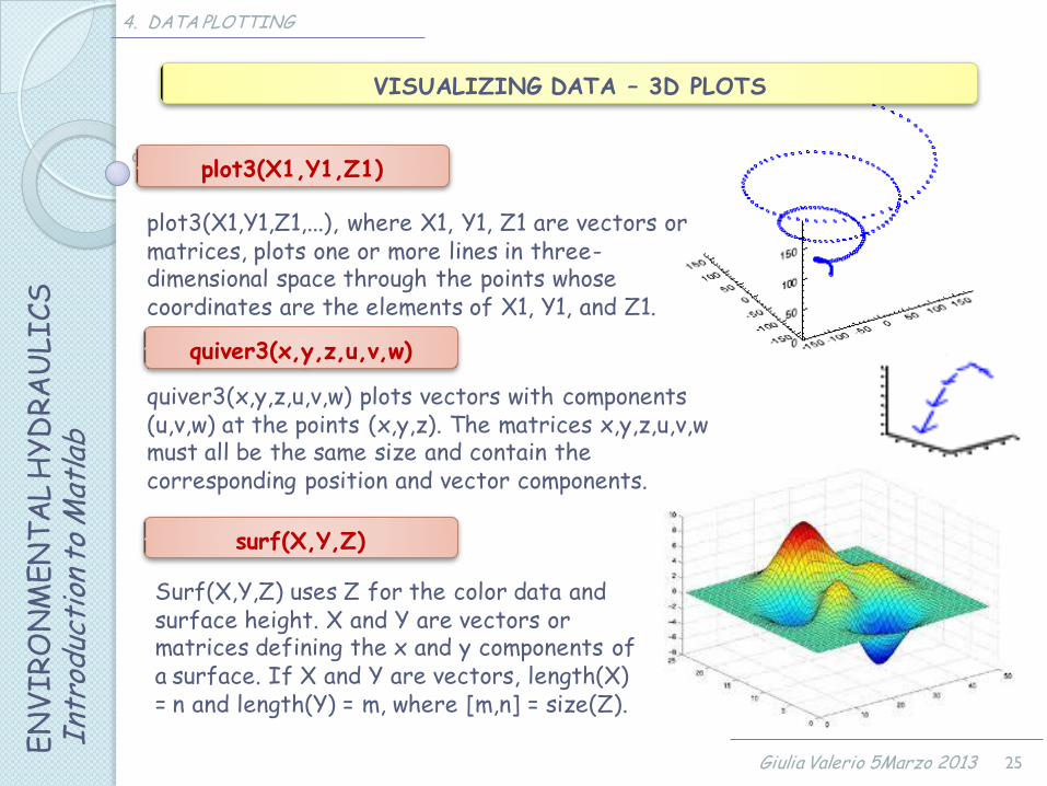
lab VISUALIZING DATA – 3D PLOTS
25 Giulia Valerio 5Marzo 2013
4. DATA PLOTTING
surf(X,Y,Z)
Surf(X,Y,Z) uses Z for the color data and surface height. X and Y are vectors or matrices defining the x and y components of a surface. If X and Y are vectors, length(X) = n and length(Y) = m, where [m,n] = size(Z).
plot3(X1,Y1,Z1)
plot3(X1,Y1,Z1,...), where X1, Y1, Z1 are vectors or matrices, plots one or more lines in three-dimensional space through the points whose coordinates are the elements of X1, Y1, and Z1.
quiver3(x,y,z,u,v,w)
quiver3(x,y,z,u,v,w) plots vectors with components (u,v,w) at the points (x,y,z). The matrices x,y,z,u,v,w must all be the same size and contain the corresponding position and vector components.

EN
VIR
ON
MEN
TA
L H
YD
RA
ULICS
I
ntro
duc
tion
to
Mat
lab
4. DATA MANIPULATION
26 Giulia Valerio 5Marzo 2013
PRACTICE
Use the previous data to create a figure (Figure 5) that shows the bathymetry of lake Iseo superimposed to the Oglio vectors
located at -10m depth