data structures, algorithms and applications for big data

University of Calgary

PRISM: University of Calgary's Digital Repository

Graduate Studies The Vault: Electronic Theses and Dissertations

2017

Data Structures, Algorithms and Applications for Big

Data Analytics: Single, Multiple and All Repeated

Patterns Detection in Discrete Sequences

Xylogiannopoulos, Konstantinos

Xylogiannopoulos, K. (2017). Data Structures, Algorithms and Applications for Big Data Analytics:

Single, Multiple and All Repeated Patterns Detection in Discrete Sequences (Unpublished doctoral

thesis). University of Calgary, Calgary, AB. doi:10.11575/PRISM/25522

http://hdl.handle.net/11023/3754

doctoral thesis

University of Calgary graduate students retain copyright ownership and moral rights for their

thesis. You may use this material in any way that is permitted by the Copyright Act or through

licensing that has been assigned to the document. For uses that are not allowable under

copyright legislation or licensing, you are required to seek permission.

Downloaded from PRISM: https://prism.ucalgary.ca

UNIVERSITY OF CALGARY

Data Structures, Algorithms and Applications for Big Data Analytics:

Single, Multiple and All Repeated Patterns Detection in Discrete Sequences

by

Konstantinos F. Xylogiannopoulos

A THESIS

SUBMITTED TO THE FACULTY OF GRADUATE STUDIES

IN PARTIAL FULFILMENT OF THE REQUIREMENTS FOR THE

DEGREE OF DOCTOR OF PHILOSOPHY

GRADUATE PROGRAM IN COMPUTER SCIENCE

CALGARY, ALBERTA

APRIL, 2017

© Konstantinos F. Xylogiannopoulos 2017

ii

Abstract

My research work of the current thesis focuses on the detection of single, multiple and all

repeated patterns in sequences. Many algorithms exist for single pattern detection that take an input

argument (i.e., pattern to be detected) and produce as outcome the position(s) where the pattern

exists. However, to the best of my knowledge, there is nothing in literature related to all repeated

patterns detection, i.e., the detection of every pattern that occurs at least twice in one or more

sequences. This is a very important problem in science because the outcome can be used for

various practical applications, e.g., forecasting purposes in weather analysis or finance by

detecting patterns having periodicity.

The main problem of detecting all repeated patterns is that all data structures used in

computer science are incapable of scaling well for such purposes due to their space and time

complexity. In order to analyze sequences of Megabytes the space capacity required to construct

the data structure and execute the algorithm can be of Terabyte magnitude. In order to overcome

such problems, my research has focused on simultaneous optimization of space and time

complexity by introducing a new data structure (LERP-RSA) while the mathematical foundation

that guarantees its correctness and validity has also been built and proved. A unique, innovative

algorithm (ARPaD), which takes advantage of the exceptional characteristics of the introduced

data structure and allows big data mining with space and time optimization, has also been created.

Additionally, algorithms for single (SPaD) and multiple (MPaD) pattern detection have been

created, based on the LERP-RSA, which outperform any other known algorithm for pattern

detection in terms of efficiency and usage of minimal resources. The combination of the innovative

data structure and algorithm permits the analysis of any sequence of enormous size, greater than a

trillion characters, in realistic time using conventional hardware.

iii

Moreover, several methodologies and applications have been developed to provide

solutions for many important problems in diverse scientific and commercial fields such as Finance,

Event and Time Series, Bioinformatics, Marketing, Business, Clickstream Analysis, Data stream

Analysis, Image Analysis, Network Security and Mathematics.

iv

Acknowledgements

Firstly, I would like to thank my PhD supervisor Professor Reda Alhajj most sincerely for

believing in my strengths and potential and for giving me the opportunity to complete my PhD at

the University of Calgary, in Canada. I also want to thank him for his constant support, inspiration

and motivation. His positive attitude to my requests for additional resources I greatly appreciated

as it helped me to achieve extraordinary research results in Computer and Data Science.

My thanks also to the other members of my PhD supervisory committee Professor Jon

George Rokne, Professor Panayote Pardalos, Dr. Jalal Kawash and Dr. Mohamed Helaoui for the

important feedback provided for my thesis and the acknowledgement of my research work. I would

especially like to thank Professor Rokne for the time we spent discussing several scientific or

general interest subjects over a cup of coffee.

I would like to thank the members of the technical office of the Computer Science

Department, Mr. Darcy Scott Grant, Mr. Gerald Vaselenak and Mr. Ryan Woo for consistently

providing significant resources whenever I needed them and keeping the computers up and running

24/7. I would also like to thank all members of the administrative and academic staff for their

constant support and help.

My thanks also to my good friend and MSc supervisor Dr. Panagiotis Karampelas for the

continuous encouragement.

Last but not least I would like to express my gratitude to my father Fotis and my brother

Leonidas for the daily communication and positive reinforcement. Their constant support was

extremely helpful in order to bypass all problems and achieve my academic goal.

vi

Dedication

To my mother Ελένη†

and my father Φώτη†

viii

Table of Contents

Abstract ........................................................................................................................................... ii

Acknowledgements ........................................................................................................................ iv

Dedication ...................................................................................................................................... vi

Table of Contents ......................................................................................................................... viii

List of Tables ................................................................................................................................ xii

List of Figures and Illustrations ................................................................................................... xiv

List of Symbols, Abbreviations, Nomenclatures ......................................................................... xvi

Chapter 1 Introduction .......................................................................................................... 1

1.1 Problem Definition ............................................................................................................... 1

1.2 Motivation ............................................................................................................................. 3

1.3 Contributions ........................................................................................................................ 4

1.4 Thesis Organization .............................................................................................................. 6

Chapter 2 Computer Science and Mathematical Background .............................................. 9

2.1 Introduction ........................................................................................................................... 9

2.2 Pattern Matching and Related Data Structures ................................................................... 10

2.2.1 Suffix Trees ................................................................................................................ 10

2.2.2 Suffix Arrays .............................................................................................................. 11

2.2.3 Pattern Matching ........................................................................................................ 13

2.3 Number Theory ................................................................................................................... 15

2.3.1 Normal Numbers ........................................................................................................ 15

2.3.2 Randomness ................................................................................................................ 18

Chapter 3 Advanced Data Structure for Pattern Detection in Big Data ............................. 23

3.1 Introduction ......................................................................................................................... 23

3.2 Perfect Periodicity ............................................................................................................... 24

3.2.1 Perfect Periodicity Theorem and Related Lemmas .................................................... 24

3.3 Full and Reduced Suffix Array ........................................................................................... 34

3.3.1 Maximum Space Required Capacity Theorem ........................................................... 36

3.4 Longest Expected Repeated Pattern (LERP) ...................................................................... 38

3.4.1 Reduced Suffix Array Maximum Space Required Capacity Theorem and Related

Lemmas ....................................................................................................................... 38

ix

3.5 Probabilistic Existence of Longest Expected Repeated Pattern Theorem and Related

Lemmas ............................................................................................................................. 42

3.6 Longest Expected Repeated Pattern Reduced Suffix Array (LERP-RSA) ......................... 63

3.7 LERP-RSA Advanced Characteristics ................................................................................ 64

3.7.1 Classification .............................................................................................................. 64

3.7.2 Parallelism .................................................................................................................. 65

3.7.3 Semi-Parallel Classification/Execution ...................................................................... 66

3.7.4 Network/Cloud Distribution and Full Parallel Execution .......................................... 68

3.7.5 Compression ............................................................................................................... 70

3.7.6 Indeterminacy ............................................................................................................. 71

Chapter 4 Advanced Algorithms for Pattern Detection in Big Data .................................. 73

4.1 Introduction ......................................................................................................................... 73

4.2 Construction of Full, Reduced and LERP-Reduced Suffix Array ...................................... 73

4.2.1 Full Suffix Array Construction (FSAC) ..................................................................... 73

4.2.2 Reduced Suffix Array LERP-RSA Construction (ORSAC) ...................................... 74

4.3 All Repeated Patterns Detection (ARPaD) Algorithms Family ......................................... 75

4.3.1 Recursive ARPaD ....................................................................................................... 76

4.3.1.1 ARPaD Algorithm Using Full Suffix Array ..................................................... 76

4.3.1.2 ARPaD Algorithm Using Full Suffix Array and Shorter Pattern Length

(ARPaD-SPL) .................................................................................................... 80

4.3.1.3 ARPaD Algorithm Using LERP Reduced Suffix Array and SPL .................... 82

4.3.1.4 ARPaD Algorithm Correction .......................................................................... 84

4.3.1.5 ARPaD Algorithm Analysis ............................................................................. 86

4.3.2 Non-Recursive ARPaD .............................................................................................. 87

4.3.2.1 N-R ARPaD Algorithm Correction .................................................................. 88

4.3.2.2 N-R ARPaD Algorithm Analysis ..................................................................... 90

4.4 Moving Longest Expected Repeated Pattern (MLERP) Algorithm ................................... 90

4.4.1 MLERP Algorithm Correction ................................................................................... 95

4.4.2 MLERP Algorithm Analysis ...................................................................................... 95

4.5 Single Pattern Detection (SPaD) Algorithm ....................................................................... 96

4.5.1 Empty Bucket Criterion .............................................................................................. 98

x

4.5.2 Crossed Minimax Criterion ........................................................................................ 98

4.5.3 String S is Random ..................................................................................................... 99

4.5.4 String S is not Random ............................................................................................. 100

4.5.4.1 Binary Search Check ...................................................................................... 100

4.5.4.2 Linear Top Down Check ................................................................................. 101

4.5.5 SPaD Algorithm Correction ..................................................................................... 102

4.5.6 SPaD Algorithm Analysis ........................................................................................ 103

4.6 Multiple Pattern Detection (MPaD) Algorithm ................................................................ 105

4.7 SPaD and MPaD Wildcards Pattern Detection ................................................................. 107

4.8 Multivariate or Multidimensional Pattern Detection (MvdPaD) ...................................... 107

Chapter 5 Testing and Verification in Diverse Scientific and Commercial Fields .......... 111

5.1 Introduction ....................................................................................................................... 111

5.2 Event Series and Time Series Analysis ............................................................................ 112

5.3 Bioinformatics .................................................................................................................. 116

5.4 Network Security .............................................................................................................. 121

5.5 Transactions Analysis ....................................................................................................... 126

5.5.1 Pre-process Analysis Phase ...................................................................................... 132

5.5.1.1 Pre-Statistical Analysis ................................................................................... 133

5.5.1.2 Transaction String Transformation ................................................................. 134

5.5.1.3 LERP-RSA Construction ................................................................................ 137

5.5.2 ARPaD Data Mining Phase ...................................................................................... 140

5.5.2.1 Frequent Sequential Itemsets Detection ......................................................... 140

5.5.2.2 Meta-Analyses of the Results ......................................................................... 141

5.6 Clickstream Analysis ........................................................................................................ 145

5.7 Data Stream Analysis ........................................................................................................ 150

5.7.1 Sequential Execution ................................................................................................ 150

5.7.2 Dynamic Execution .................................................................................................. 153

5.8 Mathematics ...................................................................................................................... 156

5.8.1 Randomness .............................................................................................................. 157

5.8.2 LERP-RSA and ARPaD Efficiency ......................................................................... 160

5.8.3 Irrational Numbers and Big Data ............................................................................. 165

xi

5.9 Image Analysis ................................................................................................................. 168

5.10 Compression ................................................................................................................... 170

5.11 Text Mining .................................................................................................................... 171

Chapter 6 Conclusions and Future Research .................................................................... 173

6.1 Synopsis ............................................................................................................................ 173

6.2 Future Research ................................................................................................................ 174

Bibliography ............................................................................................................................... 175

Appendix: Copyright Permissions .............................................................................................. 187

xii

List of Tables

Table 1 Indicative Data Results for Quartiles with Confidence Greater or Equal Than

0.75 ...................................................................................................................... 116

Table 2 Location, Dispersion and Shape Parameters for DNA string experiments ......... 119

Table 3 Theoretical and Actual LERP for DNA Strings Experiments ............................. 119

Table 4 Transactions per Itemset Length ......................................................................... 143

Table 5 Items Classification per First Decimal Digit ....................................................... 143

Table 6 Database Size ...................................................................................................... 147

Table 7 Execution Time ................................................................................................... 147

Table 8 Classification per Alphabet Digit ........................................................................ 147

Table 9 Top 20 and Bottom 10 Sequential Frequent Sizes .............................................. 148

Table 10 Top 20 More Frequent Sequential Itemsets ........................................................ 148

Table 11 Top 20 Itemsets Per Itemset Size ........................................................................ 149

Table 12 Longest Repeated Patterns per Pattern Length for 1,000 Billion digits strings

of π....................................................................................................................... 155

Table 13 Upper Bounds Comparison for Largest Repeated Substring of 1,000

experiments of 1 Billion digits strings from π..................................................... 156

Table 14 Occurrences per Pattern Length for Champerowne Constant ............................. 159

Table 15 Theoretical and Actual LERP for Champernowne Constant .............................. 159

Table 16 Location, Dispersion and Shape Parameters for Champernowne Constant

Experiments ......................................................................................................... 160

Table 17 Upper Bounds Comparison for Largest Repeated Substring of Champernowne

Constant of length 68,888,889 ............................................................................ 160

xiii

Table 18 Patterns and Cumulative Occurrences per Pattern Length for 68GB string of π 162

Table 19 Least Patterns per Pattern Length for 68GB string of π ...................................... 164

Table 20 Most Patterns per Pattern Length for 68GB string of π ...................................... 164

Table 21 Longest Repeated Pattern for 68GB string of π .................................................. 164

Table 22 Patterns and Cumulative Occurrences per Pattern Length for 1 Trillion

decimal digits string of π ..................................................................................... 167

Table 23 Longest Repeated Patterns in the first 1 Trillion decimal digits of π .................. 167

xiv

List of Figures and Illustrations

Figure 1 Suffix Tree of string kananaskis ............................................................................ 10

Figure 2 Suffix Array (SA[i]) of string kananaskis ............................................................. 12

Figure 3 Different sequences for the calculation of perfect periodicity .............................. 28

Figure 4 Original sequence for the calculation of perfect periodicity using Theorem 1 ..... 30

Figure 5 Transformed sequence for the calculation of perfect periodicity using Lemma

1 ............................................................................................................................. 30

Figure 6 Sequence for calculation of perfect periodicity using Lemma 2 ........................... 33

Figure 7 The suffix strings of the string kananaskis, the full suffix array and the reduced

suffix array of width 𝑙 = 5 < 10 = 𝑛 ................................................................... 35

Figure 8 The suffix array of string kananaskis and the part that does not need to be

stored ..................................................................................................................... 37

Figure 9 The suffix strings of string kananaskis and the Full/Reduced Suffix Array with

substrings of length at most three .......................................................................... 40

Figure 10 Possible occurrences of string ab in a 5 character long string .............................. 46

Figure 11 Possible occurrences of string ba in 5 character long string ................................. 46

Figure 12 Possible occurrences of string ab in 7 characters long string ................................ 51

Figure 13 Possible arrangements of five letters in a ten digits long string ............................ 54

Figure 14 Possible arrangements of five letters in a ten digits long string with a specific

property ................................................................................................................. 54

Figure 15 Full Suffix Array and LERP-RSA in Indeterminacy State ................................... 72

Figure 16 The repeated patterns of string kananaskis using ARPaD-FSA ............................ 79

Figure 17 The repeated patterns of string kananaskis using a ARPaD with 𝐿𝐸𝑅𝑃 = 3 ....... 83

xv

Figure 18 The Full Suffix Array of string kananaskis and the MLERP process ................... 94

Figure 19 Linear Top Down Check Method ........................................................................ 102

Figure 20 Occurrences per pattern length and Cumulative Occurrences for DNA

experiment with length n=2,000,000................................................................... 119

Figure 21 Occurrences per pattern length and Cumulative Occurrences for DNA

experiment with length n=4,000,000................................................................... 120

Figure 22 CAIDA DDoS attack from August 4, 2007, 21:50:08 UTC to 21:23:59 UTC

dataset LERP-RSA and ARPaD execution in four phases .................................. 126

Figure 23 SAFID Flow Diagram ......................................................................................... 132

Figure 24 LERP-RSA, lexicographically sorted LERP-RSA and ARPaD results .............. 144

Figure 25 Data Stream Analysis Sequential Execution ....................................................... 151

Figure 26 Data Stream Analysis Dynamic Execution for the first two subsequences ........ 153

Figure 27 Data Stream Analysis Dynamic Sliding Window Execution .............................. 154

Figure 28 Clear and unclear images of Greek letter Γ ......................................................... 169

xvi

List of Symbols, Abbreviations, Nomenclatures

ARPaD All Repeated Patterns Detection

FSA Full Suffix Array

LERP Longest Expected Repeated Pattern

LERP-RSA Longest Expected Repeated Pattern Reduced Suffix Array

MLERP Moving Longest Expected Repeated Pattern

MPaD Multiple Patterns Detection

MvdPaD Multivariate and/or Multidimensional Pattern Detection

RSA Reduced Suffix Array

SA Suffix Array

SPaD Single Pattern Detection

SPL Shorter Pattern Length

ST Suffix Tree

1

Chapter 1 Introduction

1.1 Problem Definition

The current proposed research work deals with the general problem of pattern detection in

discrete sequences. This problem has many variations, e.g., detecting single predefined patterns,

discovering a group of multiple patterns, using wildcards for the detection of more flexible patterns

etc. The use of the term “discrete” seems to restrict the problem to a very minor group of sequences

constructed from small alphabets, yet, this is not the case. Almost every sequence constructed from

continuous, real values can be transformed to discrete by applying discretization methods as seen

in [Xylogiannopoulos et al. 15a].

The specific problem of pattern detection is very important in Computer Science and more

specifically in Data Mining as it has many applications in diverse scientific and commercial fields.

In order to address this problem in the past five decades, several data structures have been

introduced in combination with many more algorithms. This blend of data structures and

algorithms has been trying to propose efficient methodologies for pattern detection that can deal

with space and time complexity. With the new era of Big Data this problem has become even more

important and more complex. Data structures and algorithms used so far for pattern detection have

been proven inefficient in scaling up in order to work with big data. Hardware limitations block

any effort towards this direction by setting an upper limit for these methodologies. Furthermore,

software limitations also exist. Operating Systems have been upgraded in 64bit mode in the past

few years breaking the barrier of 4GB memory and addressing usage. File Systems also cause

many problems when trying to deal with huge files or an enormous number of files. Programming

languages set different type of limitations related to memory addressing or usage for basic data

2

structures, which are important when building any kind of application for data mining and more

specifically pattern detection.

All other alternative methodologies which exist in literature, related to the pattern detection

problem, try to deal with the very common problem of fitting any kind of data structure in a

computer memory or disk in order to apply different, time efficient, methods for pattern detection.

The current advanced and sophisticated proposed methodology allows altering the aforementioned

general problem to a group of different problems:

1) Is it possible to break the data structure into the smallest possible partitions and

then apply pattern detection algorithms on them?

2) If so, how can this be done in the most efficient way in order to bypass hardware

and software limitations?

In the current thesis, it has been attempted to address several problems. These problems

can be defined as follows:

1) Is it possible to create a data structure that can scale up to any size of a sequence in

order to apply pattern detection algorithms without facing hardware or software

limitations?

2) Using the proposed data structure can an algorithm detect all repeated patterns that

exist in the sequence in efficient time?

3) Is it possible to construct single and multiple pattern detection algorithms which

can outperform others using the proposed data structure?

4) Is it possible to use these algorithms and data structures to perform multivariate and

multidimensional pattern detection?

3

5) How can the proposed data structure and algorithms be used to solve important,

real-life, problems in scientific and commercial fields?

All these problems will be answered in the current thesis by first establishing the

mathematical foundation which will prove the validity, originality and efficiency of the proposed

methodology. A new data structure will be introduced, which can scale up to any size using

standard computer systems or even simple electronic devices such as smartphones. An innovative

algorithm which can detect all repeated patterns will be presented for the first time in literature,

after being published in prestigious journals and conference proceedings. Furthermore, single and

multiple pattern detection algorithms will be presented which can outperform alternative

algorithms which exist in literature so far with the use of the proposed data structure, while the

problem of multivariate and multidimensional pattern detection will also be addressed.

1.2 Motivation

The motivation behind this research work is to be able for the first time to create an

algorithm that can detect all repeated patterns in a sequence. To the best of my knowledge and

based on the literature research conducted, such an algorithm does not exist so far. Therefore, it is

very important because besides the obvious usage of helping periodicity detection algorithms to

detect possible periodic patterns and use them for forecasting purposes, it will also be presented

that it can be extremely useful when dealing with real-life problems which may seem irrelevant to

the general concept of the problem. For example, the proposed methodology has so far been

applied to network security, transactions analysis, clickstream analysis, data stream analysis,

Number Theory and many more areas with extraordinary results.

4

Moreover, although the algorithm has been created first during this research work and

behaved very well, very soon it faced the usual problems that all algorithms have when dealing

with big data mining problems; hardware and software limitations. In order to bypass these

limitations, the need for a new, more efficient data structure which can scale up with the fewest

possible resources was important for my research work. This led to the creation of a novel, very

powerful and flexible data structure that can outperform any other known data structure in

literature so far. This data structure allows the analysis of any size sequence with limited hardware

resources when other data structures simply cannot scale up to addressing big data problems.

1.3 Contributions

The current thesis makes many significant contributions to Computer and Data Science,

which can be enumerated as follows:

1) It provides the correct formula for Perfect Periodicity calculation (§ 3.2)

2) It introduces the concept of Longest Expected Repeated Pattern (LERP), which

allows the linear space required capacity construction of the Full Suffix Array (§

3.4)

3) It introduces the Probabilistic Existence of Longest Expected Repeated Pattern

Theorem, which will allow the estimation of the LERP value given a probability to

exist and without any previous knowledge regarding the sequence apart from its

core characteristics, i.e., the length and the alphabet which has been used to

construct the sequence (§ 3.5)

4) It introduces a new data structure, the Longest Expected Repeated Pattern Reduced

Suffix Array (LERP-RSA), which uses the actual suffix strings of a sequence. It is

5

an augmented version of the suffix array to satisfy the performance target of

simultaneous optimization of time and space complexity and overcome all the

discouraging characteristics of the traditional data structures (§ 3.6)

5) It recognizes and illustrates unique attributes of the LERP-RSA data structure

which enable the LERP-RSA to scale up with limited resources in order to analyze

sequences of enormous sizes (§ 3.7)

6) It introduces the novel algorithm All Repeated Patterns Detection (ARPaD), which

can detect all repeated patterns in a sequence in loglinear time complexity using

LERP-RSA (§ 4.3)

7) It introduces the novel algorithm Moving Longest Expected Repeated Pattern

(MLERP), which allows the detection of all repeated patterns regardless of size and

hardware limitations using LERP-RSA and ARPaD (§ 4.4)

8) It introduces the novel algorithm Single Pattern Detection (SPaD), which allows

the detection of single patterns in constant time complexity using LERP-RSA (§

4.5)

9) It introduces the novel algorithm Multiple Pattern Detection (MPaD), which allows

the detection of multiple patterns in constant time complexity using LERP-RSA (§

4.6)

10) It presents how SPaD and (MPaD) can be used for efficient wildcard patterns

detection (§4.7)

11) It presents a novel methodology for Multivariate and Multidimensional Pattern

Detection (MvdPaD) using LERP-RSA and ARPaD, SPaD and MPaD algorithms

(§4.8)

6

12) It introduces novel approaches, methodologies and solutions to several very

important problems in many diverse scientific and commercial fields such as:

a) Event and Time Series Analysis (§ 5.2)

b) Bioinformatics (§5.3)

c) Network Security (§5.4)

d) Transactions Analysis (§5.5)

e) Clickstream Analysis (§5.6)

f) Data Stream Analysis (§5.7)

g) Mathematics and Number Theory (§5.8)

h) Image Analysis (§5.9)

i) Compression (§5.10)

j) Text Mining (§5.11)

k) Multivariate and Multidimensional Pattern Detection (§5.4, §5.5, §5.6, §5.9

& §5.11)

1.4 Thesis Organization

The thesis is organized as follows. Chapter 2 covers the existing literature related to the

two data structures widely used for sequence analysis, namely Suffix Trees and Suffix Arrays.

Chapter 2 also covers the existing literature in Mathematics and more specifically in Number

Theory regarding Normal Numbers and Randomness, which will be used as the foundation of the

proposed methodology. Chapter 3 covers the theoretical foundation of the thesis. The first part

covers the Perfect Periodicity concept while the second introduces the new data structure Reduced

Suffix Array. Furthermore, the notion of Longest Expected Repeated Pattern (LERP) is introduced.

7

The core theorem of the thesis regarding the calculation of the length of the LERP is presented and

proved while the Lemma for the estimation of LERP is also presented. Finally, advanced

characteristics of the novel LERP-RSA data structure are presented and discussed. Chapter 4

presents the algorithms for the LERP-RSA construction, the All Repeated Patterns Detection

algorithm family including the Moving LERP algorithm. Furthermore, two more algorithms are

introduced, the Single Pattern Detection and the Multiple Pattern Detection. Chapter 5 presents the

testing and verification of the newly introduced LERP-RSA data structure and ARPaD algorithm.

Moreover, new approaches, methodologies and solutions to several scientific and commercial

problems that can be addressed with the use of LERP-RSA and ARPaD are also presented and

discussed. Chapter 6 covers the conclusions and future research work plans. Finally, bibliography

with a full list of references used completes the thesis.

9

Chapter 2 Computer Science and Mathematical Background

2.1 Introduction

Before describing the fundamental theoretical aspects of the currently proposed research

work it is important to make a distinction between sequences and strings. In mathematics, the term

sequence refers to an ordered collection of objects, usually named elements or members of the

sequence. Furthermore, sequences are usually infinite deriving, e.g., from a function or a series.

The most important characteristics are that the elements of the sequence are ordered and repetitions

are allowed in contrast to sets where these two attributes are not allowed.

The term string is usually used in Computer Science in order to describe a sequence of a

fixed length constructed from alphanumeric characters. Therefore, in contrast to sequences, strings

are finite and can be constructed from sequences by extracting a specific, finite, part from them.

For example, the results of the coin flip after one hundred flips build a string while the decimal

digits of an irrational number form a sequence due to infinity, yet, in both cases the elements are

ordered and repetitions are allowed. However, the sequence can be transformed to a string by

selecting a specific number of consecutive digits from its infinite digits collection.

Both terms will be used here depending on the theory that is elaborated. Although sequence

will be used when mathematical aspects are covered and string when the text describes views from

computer science, in general both terms in practise refer to the same general concept.

Part of the material covered in this chapter has been published in fully refereed journals

[Xylogiannopoulos et al. 14a, 14b, 16b].

10

2.2 Pattern Matching and Related Data Structures

2.2.1 Suffix Trees

The suffix tree of a string is a tree data structure that includes all the suffixes of the string

and it is considered to be a very powerful data structure (Figure 1). It is heavily used for data

mining and string analysis because of its flexibility in string processing [Gusfield 97, Elfeky et al.

05, Cheung et al. 05]. Many algorithms have been developed in the past decades to create suffix

trees, including Weiner [Weiner 73] and McCreight [McCreight 76], with 𝑂(𝑛2) and 𝑂(𝑛 𝑙𝑜𝑔 𝑛)

time complexity, respectively. A suffix tree can also be created in linear time using Ukkonen’s

latest algorithm [Ukkonen 95] with the assumption that it can be stored in main memory [Gusfield

97, Cheung 05]. Then, several other algorithms can be used to traverse suffix trees such as the non-

recursive algorithm for binary search tree traversal [Al-Rawi et al. 03]. Moreover, many techniques

have been developed to store the suffix trees on secondary storage, i.e., disk [Gusfield 97, Cheung

05].

Figure 1 Suffix Tree of string kananaskis

11

Nevertheless, performance problems might occur when traversing the tree, especially if the part

that is to be processed is not loaded entirely in memory. In any case, such methods are very useful

for processing large sequences and their strings [Cheung 03], such as traffic control systems, DNA

analysis in bioinformatics, etc.

Despite the linear time complexity, many of the methods used in the construction of suffix

trees are very time consuming, especially if the sequences to be analyzed are very long [Cheung

05, Tian et al. 05]. Moreover, for very long sequences, in which the whole structure has to be

stored on disk instead of memory, significant issues could occur. The constant disk access for

writing and reading data can reduce the performance of the algorithm to a great extent [Tian et al.

05]. However, the linear time construction and the lesser space consumption compared to other

data structures have established suffix trees as the preferable data structure for various string

matching analysis tasks [Cheung 05, Tian et al. 05]. Despite that, a number of researchers have

shown that it is unfeasible to construct a suffix tree that exceeds the available main memory, e.g.,

[Navarro and Baeza-Yates 99, Navarro and Baeza-Yates 00]. To overcome this problem, new

techniques have been introduced recently, e.g., [Gusfield 97, Cheung et al. 05, Phoophakdee 07,

Phoophakdee and Zaki 07, Barsky et al. 11], that allow for the analysis of the data to be stored

outside the main memory. Such techniques lead to a significant improvement in the performance

of suffix tree processing and turn them into a powerful data structure.

2.2.2 Suffix Arrays

A suffix array is an array of the lexicographically sorted suffices of a sequence. As it has

been introduced by Manber and Myers in 1990 [Manber and Myers 90], a suffix array is an array

of integers declaring the starting position of all, lexicographically sorted, suffices of a string, not

12

including the actual suffix strings (Figure 2). A suffix array can be constructed in 𝑂(𝑛 log 𝑛) time

in the worst case, including the longest common prefix information as Manber and Myers proposed

[Manber and Myers 90]; this is mainly due to the sorting process that is needed using the merge-

sort algorithm.

Recently, more researchers such as Schürmann and Stoye [Schürmann and Stoye 05] and

Karkkainen et al. [Karkkainen et al. 06] introduced more efficient, linear methods for fast suffix

array creation, while Ko and Aluru [Ko and Aluru 03] produced a linear complexity algorithm for

sorting specific types of suffix arrays. Suffix arrays do not suffer from the memory storage problem

since they can be stored and accessed directly from external media such as hard disks. However,

the read-write I/O process is very time consuming compared to the direct access in main memory.

For large sequences, this can be a significant drawback which sometimes forbids the analysis of

such sequences. Moreover, suffix arrays may need less storage capacity compared to the size and

the expected space of other structures, especially when the alphabet is very large [Manber Myers

90, Sinha et al. 08]. On the other hand, a disadvantage of suffix arrays compared to suffix trees is

the huge amount of data that should be stored if the full suffices have to be stored as well.

Figure 2 Suffix Array (SA[i]) of string kananaskis

So far, the main efforts of researchers who have used suffix arrays and trees have focused

on the optimization of the construction time, e.g., [Kim et al. 03, Wong et al. 07, Dementiev et al.

08] and more specifically on constructing the structure with linear time complexity [Ko and Aluru

03, Kim et al. 03]. Many techniques have been introduced that focus on the Longest Common

13

Prefix (LCP) [Crauser and Ferragina 02, Ko and Aluru 03, Kim et al. 03], denoted lcp(a,b), which

is the longest common prefix between two strings a and b.

2.2.3 Pattern Matching

Based on the data structures mentioned above, many algorithms have been constructed for

pattern detection and matching. Suffix trees have been used for several decades to address

fundamental string problems, e.g., detecting all repetitions in a string [Apostolico and Preparata

83] or the longest repeated substring [Weiner 73]. Karlin et al. [Karlin et al. 83] also proposed a

formula for estimating the size of the longest repeated substring, which exists in some variations

based on a suffix tree’s height [Apostolico and Szpankowski 92, Devroye et al. 92, Manber and

Myers 90]. Especially for the suffix array, when it includes information regarding the longest

common prefixes of the adjacent elements, searches for a string S can be done in 𝑂(|𝑆| + log 𝑛),

where |𝑆| is the length of string S [Manber and Myers 90]. Moreover, several researchers have

published a plethora of techniques using suffix arrays and suffix trees for DNA or text analysis.

Such papers have been published lately proposing different disk-based techniques capable of

analyzing suffix arrays and suffix trees, e.g., [Phoophakdee and Zaki 07, Sinha et al. 08, Orlandi

and Venturini 11, Gog et al. 13] where the researchers propose techniques that combine suffix

trees and suffix arrays.

In addition to the effort of introducing the suffix array, Manber and Myers also created an

algorithm for fast detection of the presence of a specific string inside a large text [Manber and

Myers 90]. Variations of this method exist such as [Franek et al. 03] in which Franek, Smyth and

Tang introduced a methodology for the detection of repeats using suffix arrays. The specific

methodology can identify repeats of substrings that satisfy specific conditions regarding period,

14

proximity or minimum length [Franek et al. 03]. Moreover, this method has been analyzed

experimentally for the first time in [Puglishi et al. 08] where Puglishi, Smyth and Yusufu analyzed

strings up to just 68 million characters.

Another need for the use of suffix trees and suffix arrays is the identification of periodicities

in the detected repeated patterns. There are many algorithms that can be used for the analysis of

sequences and the detection of periodicities [Elfeky et al. 05b, Rasheed and Alhajj 08, Rasheed et

al. 10]. Elfeky et al. in their work, proposed two distinct algorithms for symbol and segment

periodicity with complexity 𝑂(𝑛 𝑙𝑜𝑔 𝑛) and 𝑂(𝑛2), respectively [Elfeky et al. 05b]. Their main

difference is that the former does not function properly in the presence of insertion or deletion

noise, i.e., when parts of the time series are deleted or new parts have been imported into the series

during the analysis. However, the latter introduced algorithms of Rasheed et al. [Rasheed et al. 10]

are noise resilient by allowing deletions and insertions during the analysis phase and with time

complexity 𝑂(𝑛2). Many other algorithms have been developed lately using several techniques,

such as Han et al. [Han et al. 99] for partial periodicity and multiple periods data mining in time

series, with a prerequisite that the user should provide the expected period value for which the

algorithms will check for periodicity. Based on this algorithm Sheng et al. [Sheng et al. 05, 06]

developed a variation to detect periodic patterns in a section of a time series by an optimized

method. Their method can find a dense periodic range inside time series in 𝑂(𝑛) when the expected

periodic value is provided, otherwise its complexity could rise to 𝑂(𝑛2). Moreover, Huang and

Chang [Huang and Chang 05] also developed an algorithm for asynchronous periodic patterns. In

their case, occurrences can be shifted along the time axis in a small range and their method still

uses 𝑂(𝑛2) time complexity.

15

2.3 Number Theory

In order to answer the questions of paragraph 1.1, which are related to the construction of

a hardware and software efficient data structure, the Probabilistic Existence of Longest Expected

Repeated Pattern Theorem will be proved in paragraph 3.5. However, in order to accomplish that

proof, two very important mathematical concepts have to be introduced before continuing, i.e., the

normality of irrational numbers and randomness. These two notions are interrelated and are very

important in order to provide an efficient and accurate estimation of the longest pattern that can

exist in a string using only the basic attributes of the string, i.e., its length and the alphabet that has

been used to construct it. The previously mentioned Theorem of paragraph 3.5 assumes that the

string under analysis should be Random and, therefore, Normal [Calude 94], two concepts that

will be thoroughly discussed in the following sub-paragraphs.

2.3.1 Normal Numbers

Every real number can be expressed based on the digits of the base from which it is

constructed. For example, the rational number 𝑎 =2

3 can be expressed in binary form as 𝑎 =

0.101010 ∙∙∙, with base 𝑏 = {0,1}, while in decimal form as 𝑎 = 0.6666 ∙∙∙, with base 𝑏 =

{0, 1, 2, 3, 4, 5, 6, 7, 8, 9}. In 1909, Émile Borel introduced the concept of normal numbers and

simultaneously proved that almost all real numbers are absolutely normal [Borel 09]. A real

number is said to be Simply Normal in the scale of a base 𝑏 if the limit of the occurrences of a digit

𝑑, of every digit of base 𝑏, in the first 𝑛 places is expressed as:

lim𝑛→∞

𝑁(𝑑, 𝑛)

𝑛=1

|𝑏|

where 𝑁(𝑑, 𝑛) means the number of 𝑏’s and |𝑏| is the cardinality of base 𝑏 [Niven and Zuckerman

51, Davemport and Erdös 52, Long 57, Khoshnevisan 06]. A real number is said to be Normal in

16

the scale of 𝑏 if every digit of base 𝑏 and the combination of digits occur in the sequence of digits

with the appropriate frequency. In this case, the limit will be:

lim𝑛→∞

𝑁(𝑆, 𝑛)

𝑛=

1

|𝑏||𝑆|

where 𝑆 is any combination of digits and |𝑆| is the length of the sequence of digits [Niven and

Zuckerman 51, Davemport and Erdös 52, Long 57, Khoshnevisan 06, Koninck 14].

For example, in the case of a decimal base, every single digit has one tenth probability to

occur (or has to occur with frequency one tenth), every combination of two digits has the

probability to occur one hundredth, etc. A real number is said to be Absolute Normal if it is normal

in every base [Niven and Zuckerman 51, Long 57]. Borel was also the first to conjecture that all

irrational algebraic numbers are b-normal for every integer 𝑏 ≥ 2, where 𝑏 is the base of the

numeric expression [Hardy and Wright 60, Bailey et al 12]. The most common bases are 2 for

binary, 10 for decimal, 16 for hexadecimal, etc. Furthermore, Borel stated and proved in 1909

[Borel 09, Hardy and Wright 60, Khoshnevisan 06] the Normal Numbers Theorem which states

that almost all real numbers are normal in any scale of 𝑏. In addition, eight years later Sierpinski

gave one more alternative proof that almost all real numbers are normal [Sierpiński 17, De Koninck

14].

Despite the very clear statement of the Normal Number Theorem, it is almost impossible

to prove normality for any of the known mathematical constants, e.g., 𝜋, 𝑒, √2, 𝜑, etc. [Wagon

85, Bailey et al. 01, 02, 12, Khoshnevisan 06, Becher 12, De Koninck 14]. For the past hundred

and more years, mathematicians have been trying to find a way to prove if a number is normal or

not. However, this has been proven to be extremely difficult due to the nature of irrational numbers

(e.g., √2) and more specifically transcendental numbers, i.e., not a root of a non-zero polynomial

17

equation with rational coefficients, like 𝜋 = ∑1

16𝑘(

4

8𝑘+1−

2

8𝑘+4−

1

8𝑘+5−

1

8𝑘+6)∞

𝑘=0 [Bailey et al.

97]. The main difficulty is that such numbers have infinite, aperiodic decimals digits and,

therefore, it is impossible to know how they will be developed through infinite digits to calculate

the frequency of each digit and the combination of digits in the sequence of decimal numbers. Yet,

there are some latest publications of Bailey et al. [Bailey et al. 12] in which, based on

computational processes, they have tried to examine if the digits of π are randomly distributed and

whether the mathematical constant π is a simply normal number. Despite their great effort and

significant work, an absolutely confirmative answer to the question whether π is a simple normal

number has not been given, yet. However, Bailey et al. managed to prove that specific bits’ length

prefixes are normal when viewed as binary word [Bailey et al. 12]. By using the specific results,

they have shown [Bailey et al. 12] that “the decision “π is not normal” has credibility […] 4.3497 ∙

10−3064” (p.382), something which could be considered as an astonishing achievement.

Moreover, based on the methodology proposed in the current thesis and by conducting

several experiments on sequences of length from 100 million digits up to 1 trillion digits, for the

first time it has been shown experimentally that the irrational numbers π, e, φ and √2, behave as

normal numbers [Xylogiannopoulos et al. 14a, 16b]. Furthermore, in the specific paper

[Xylogiannopoulos et al. 14a] it has been conjectured, based on the experimental findings, that the

irrational numbers π, e, φ and √2 are normal in decimal base (i.e., all appropriate arrangements of

digits occur for the infinite sequence of decimal digits) and not simply normal as it has been

probabilistically shown by Bailey et al. [Bailey et al. 12].

The problem of identifying a normal number was bypassed by Champernowne in 1933

[Champernowne 33] when he proved that the decimal number ∙ 123456789101112⋯,

constructed from the sequence of natural numbers, counting from 1 upwards, is normal in the scale

18

of ten. This proof is a great help when normality has to be cross-examined since it was and still is

almost impossible to prove if a number is normal. In advance of Champernowne’s constant,

Copeland and Erdös [Copeland and Erdös 46] have proved that also the sequence of prime numbers

up to a large N is also a normal number. They also conjectured that a decimal constructed by

specific polynomial is also normal, something that was proved by Davenport and Erdös

[Davenport and Erdös 52]. A few years later, Cassels [Cassels 59] for the first time presented a

large family of simply normal numbers while many more mathematicians continue to investigate

Normal Numbers and their properties [De Koninck 14].

2.3.2 Randomness

By introducing the normality of numbers, Borel and other mathematicians were actually

trying to approach the concept of randomness. A well-known approach regarding the definition of

randomness was presented by Laplace in 1819 [Calude 95, Dasgupta 11] with the following

example. The problem he was trying to address had to do with fair coin finite flips. Imagine that

we flip a fair coin fifty times and we mark each occurrence of tails with 0 and each occurrence of

heads with 1. After conducting the experiment twice, let us assume that we get two sequences (or

strings) of 0’s and 1’s like the following:

1011001011111101010001011100101001010111101010010011100010110010

0000000000000000000000000000000000000000000000000000000000000000

The first is an “arbitrary” sequence of 0’s and 1’s and the second is fifty 0’s. By arbitrary

we define any combination of 0’s and 1’s that seems to be random and will not allow us to suspect

that the coin is not fair. The first flip sequence seems to be “random” while the second not (actually

the first thing that comes to mind is that the coin is not fair). From a probabilistic point of view,

19

both sequences have the same probability of occurring, so, it should not be such a unique incident.

However, the extraordinary sequence of fifty 0’s has a probability of occurring 1 out of 250, while

fifty flips of the coin can produce a vast amount of any kind of “arbitrary” sequences such that

each sequence has of course the same probability of occurring, i.e., 1 out of 250. Calude [Calude

95] described the above incident as: “non-random strings are strings possessing some kind of

regularity, and since the number of all these strings (of a given length) is small, the occurrence of

such a string is extraordinary.” (p. 49) Therefore, we may describe such strings with a “cause”

behind them (i.e., strings attributed to a cause) as non-random while all others as random [Dasgupta

11].

The first to formulate a definition of randomness in the early 1960’s were the

mathematicians Chaitin and Kolmogorov. The basic idea behind their approach is that some binary

sequences can be algorithmically compressed into much shorter sequences, due to a specific

pattern or rule which they follow [Chaitin 88]. Such sequences are definitely not random, while

all others, which are incompressible, are said to be random [Chaitin 88]. Furthermore, in the

example of the coin flip, there is no specific strategy that someone can follow in order to have

more correct than false predictions on the occurrences of heads or tails, in order to have a betting

advantage in the long run [Church 40, Dasgupta 11]. Based on these, randomness in sequences can

be defined in three ways which, although they seem completely different, are equivalent. Dasgupta

[Dasgupta 11] describes these three approaches to defining randomness in sequences as:

1) Unpredictability, meaning that it is impossible to define a gambling strategy which

in the long run will give a successful outcome to the player,

2) Typicality, meaning that if a sequence has a special property then it cannot be

random and

20

3) Incompressibility, meaning that a finite sequence cannot be compressed to less than

almost the original length.

All three approaches are equivalent [Dasgupta 11] since for example a periodic decimal number

like 0. 3̅ is not unpredictable (we always know which is the next digit), has a special property (is

periodic) and can be easily compressed (a sequence of infinite digits of 3).

What is important though with randomness, is what Calude describes [Calude 95] as “true

random” string: “In a “true random” string each letter has to appear with approximately the same

frequency, namely 𝑄−1. Moreover, the same property should extend to “reasonably long”

substrings.” (p. 59) What Calude proved [Calude 94] is that “every random sequence is Borel m-

normal, for every 𝑚 ≥ 1” (p. 119) Calude has proved that the equi-distribution of each letter of

an alphabet from which a sequence has been constructed, although it is a necessary condition for

randomness, is not sufficient; and, furthermore, the sequence should behave as Borel normal.

Additionally, Calude proved [Calude 94] that “almost all random strings […] do satisfy a Borel

normality-like property.” (pp. 113-114)

For the estimation of the largest repeated substring, Karlin et al. [Karlin et al. 83] proposed

the following formula in 1983:

𝐿𝑛∗ =

2 log 𝑛

log (1𝜆)− [1 +

log(1 − 𝜆)

log 𝜆+0.5772

log 𝜆] +log 2

log 𝜆

where 𝐿𝑛∗ is the length of the expected largest direct repeat, 𝜆 = ∑ 𝑝𝑖

2𝑟𝑖=1 , r is the number of letters

of the alphabet and 𝑝𝑖 the probabilities of getting the letter 𝐴𝑖 , 𝑖 = 1,2, … , 𝑟. However, it is

important to mention that in the specific publication in which the formula was introduced there is

no mathematical proof or any implication from which the formula can be derived. Based on the

formula described, other variations exist like in [Manber and Myers 90] in which the expected

21

length of the longest repeated substring is defined as 𝑂 (log𝑁

log|𝛴|), where N is the length for a text A

over an alphabet Σ. Moreover, in [Apostolico and Szpankowski 92] and [Devroye et al. 92] the

largest repeated substring is extracted by the bound of the average height for a random suffix tree

as 2 log𝑎 𝑛 + 𝑂(1), where 𝑎 = 𝑝𝑚𝑎𝑥−1 in the first case and 𝑂 (

2log𝑛

log1

∑ 𝑝𝑖2

𝑖

) in the second and 𝑂(1) is

an arbitrary constant. In all cases the randomness of the string is not defined; it is rather implied

as the equi-distribution of alphabet digits. However, in [Manber and Myers 90], based on [Karlin

et al. 83], randomness is defined as the assumption that all strings of length N are equally likely

and asking for the probability of each letter to occur in the string [Karlin et al. 83]. However, this

is not a sufficient condition to characterize a string as random as Calude has proved with his

theorem [Calude 94]. We will give a very simple counter-example by assuming that from the set

containing all strings of length N, constructed from an alphabet of four letters, we chose one

randomly. Since all strings are equally likely to be selected we may simply select the string in

which each letter occupies a continuous fragment of length k characters of the string, while all

fragments have equal size as follows:

𝑎…𝑎⏟ 𝑘

𝑏…𝑏⏟ 𝑘

𝑐 … 𝑐⏟𝑘

𝑑 …𝑑⏟ 𝑘

where 4𝑘 = 𝑛. In this case, the letters of the alphabet are equidistributed in the string, which

partially satisfies the randomness definition. However, based on the randomness definition by

Calude, the specific string is not random since it does not satisfy “Borel normality-like property”

as well [Calude 94]. Of course, the proposed formulae for the estimation of the largest repeated

substring in [Karlin et al. 83, Manber and Myers 90, Apostolico and Szpankowski 92, Devroye et

al. 92] will not provide any reasonable value for the longest repeated substring. In the specific

example, the largest repeated substring has length 𝑘 − 1 if we take into consideration the

22

overlapping; if not, it has 𝑘

2 when k is even or ⌊

𝑘

2⌋ if k is odd. To give a simpler numerical example,

let us assume that 𝑘 =12,000 so the total string length will be 𝑛 = 48,000 (like λ phage experiment

in [Karlin et al. 83]). Although in [Karlin et al. 83] the expected largest repeated substring is 14.80,

from the above described theoretical experiment we can observe very easily that the largest

repeated substring is 11,999 characters long if we allow overlapping; for the first substring (for

letter a) the starting position is 1 and the end position is 11,999, and for the second the starting

position is 2 and the end position 12,000; the same is valid for each one of the other three letters

in their relative positions. If we don’t allow overlapping, then the length of the largest repeated

substring for each one of the letters is 6,000.

It is important to mention that for all the above described methods and formulae, there are

no mathematical proofs found in the literature that will satisfy them. Therefore, it is important for

a theorem to be constructed and to provide a formula for the calculation of an upper bound of the

longest expected repeated pattern that can exist in a sequence based on specific probability and the

assumption of randomness for the sequence by using only sequences’ core characteristics, i.e., its

length and alphabet. Furthermore, it will also be proven experimentally that all these formulae fail

to give an accurate estimation for the longest expected repeated pattern.

23

Chapter 3 Advanced Data Structure for Pattern Detection in Big Data

3.1 Introduction

Usually the need to detect repeated patterns is based on the meta-analyses for periodicities

of the specific patterns and due to the absence in literature of an accurate formula for the

calculation of the perfect periodicity of a pattern in a string, Theorem 1 has been constructed and

proved. The construction and proof of the Theorem 1 is also very important in order to show why

the commonly used formula in literature to calculate the Perfect Periodicity PP of a pattern X,

𝑃𝑃(𝑝, 𝑠𝑡𝑃𝑜𝑠, 𝑋) =|𝑇|−𝑠𝑡𝑃𝑜𝑠+1

𝑝, where p is the period, stPos is the starting position of X and |𝑇| the

length of the string, like in [Nishi et al. 13, Chanda et al. 15] is inaccurate since it covers only the

special case of patterns with length one.

Based on the aforementioned Theorem, the Longest Expected Repeated Pattern (LERP)

will be defined and a new data structure, the Reduced Suffix Array (RSA) will also be introduced

in the current chapter. Furthermore, the Probabilistic Existence of Longest Expected Repeated

Pattern Theorem will be proved in order to allow us an accurate calculation of the LERP value.

The combination of the LERP and the RSA will lead to the construction of the Longest Expected

Repeated Pattern Reduced Suffix Array (LERP-RSA) data structure which is the fundamental data

structure on which several algorithms will also be introduced later. The LERP-RSA will be

presented in depth, listing several important and unique properties which it incorporates, making

it an extraordinary tool for pattern detection in any kind of big data.

Part of the material covered in this chapter has been published in fully refereed journals or

presented in conferences and published in the corresponding proceedings [Xylogiannopoulos et al.

12a, 12b, 12c, 14a, 14b, 16b].

24

3.2 Perfect Periodicity

This theorem will not only provide the formula for the calculation of perfect periodicity

but it will also lead to the construction and the proof of Theorem 2, which allows the calculation

of the maximum space required capacity of the Reduced Suffix Array.

Definition 1. (Perfect Periodicity) Consider a string 𝑆 = {𝑒0𝑒1…𝑒𝑛−1} of 𝑛 ∈ 𝑁∗elements and

length |𝑆| = 𝑛 and a substring 𝑠 = {𝑒𝑖𝑒𝑖+1…𝑒𝑖+𝑘−1}, of the string 𝑆, of 𝑘 ∈ 𝑁∗ elements and length

|𝑠| = 𝑘 that occurs starting at position 𝑖 where 0 ≤ 𝑖 ≤ 𝑖 + 𝑘 − 1 ≤ 𝑛 − 1. We define as Perfect

Periodicity 𝑃𝑃 of the substring 𝑠, with period 𝑝 ∈ 𝑁, 𝑝 ≥ 1, the maximum number of repetitions

that 𝑠 can have with period 𝑝 in the string 𝑆 without overlapping.

3.2.1 Perfect Periodicity Theorem and Related Lemmas

Theorem 1. (Calculation of Perfect Periodicity) Consider a sequence 𝑆 = {𝑒0𝑒1…𝑒𝑛−1} of

𝑛 ∈ 𝑁∗elements and length |𝑆| = 𝑛 and a substring 𝑠 = {𝑒𝑖𝑒𝑖+1…𝑒𝑖+𝑘−1}, of 𝑆, of 𝑘 ∈ 𝑁∗

elements and length |𝑠| = 𝑘. The Perfect Periodicity 𝑃𝑃 of 𝑠 with period 𝑝 ∈ 𝑁, 𝑝 > 1, can be

derived from the formula:

𝑃𝑃 = [|𝑆| + (𝑝 − |𝑠|)

𝑝]

Proof:

From the definition of the Perfect Periodicity we have, 𝑃𝑃 is the maximum number of

repetitions that a substring can have in a string. Therefore, assuming perfect periodicity we can

write:

|𝑆| = 𝑝 ∙ 𝑃𝑃 (1)

25

However, the formula is not complete because there are cases in which we can have a

residual that we have to add to the multiplication to get the precise value of the length of the string.

Therefore, we can write:

|𝑆| = 𝑝 ∙ 𝑃𝑃 + 𝑅 (2)

where 𝑅 is the residual.

From the algorithm of division between two natural numbers 𝐷 and 𝑑, where 𝐷 is the

dividend and 𝑑 the divisor, we have:

𝐷 = 𝑑 ∙ 𝑞 + 𝑟 (3)

where 𝑞 = 𝑞𝑢𝑜𝑡𝑖𝑒𝑛𝑡, 𝑟 = 𝑟𝑒𝑚𝑎𝑖𝑛𝑑𝑒𝑟 and 𝑞, 𝑟 ∈ 𝑁.

Comparing equations (2) and (3) we can notice that they are analogous. Variables in the

two equations correspond to each other as follows:

𝐷 ≡ |𝑆|

𝑑 ≡ 𝑝

𝑞 ≡ 𝑃𝑃

and

𝑟 ≡ 𝑅

From this result, we can claim that perfect periodicity derives from the algorithm of

division since the divisor has exactly the same definition as periodicity, while the quotient is the

same outcome as perfect periodicity. Indeed, with the divisor 𝑑 we divide the dividend 𝐷 and get

a quotient 𝑞, while if we divide |𝑆| with the period 𝑝 (the divisor) we will get 𝑃𝑃 (the quotient),

plus any remainder.

In the case of perfect periodicity, it is important to note that perfect periodicity 𝑃𝑃 is larger

than the quotient 𝑞 by one when the remainder of the division is not 0 (if 𝑟 ≠ 0, we do not have

26

perfect division), so, we have to change the equation 𝑃𝑃 ≡ 𝑞 to 𝑃𝑃 = 𝑞 + 1 ⇒ 𝑞 = 𝑃𝑃 − 1. That

is because while in the division between two natural numbers we get as a result the quotient that

gives us the integral times that 𝐷 is greater than 𝑑 (plus a remainder, if any), in periodicity we have

to count also the first occurrences of the substring 𝑠. Namely, we analyze substrings with a length

of at least 1 and therefore the substring itself takes space inside the string, which is not the case of

the division between natural numbers. For example, in the division 10/5 we will get as quotient 2

and remainder 0, while in the sequence 𝑆1 = {𝑎 ∗∗∗∗ 𝑎 ∗∗∗∗} with length 10 we have again two

occurrences of the substring 𝑠 = {𝑎}, at positions 0 and 5, with period 5 and a residual of 4

elements. In this case, we have perfect division and that is why perfect periodicity is equal to the

quotient. If we expand the sequence 𝑆1 by adding one more element and create a new sequence,

say 𝑆2 = {𝑎 ∗∗∗∗ 𝑎 ∗∗∗∗ 𝑎} then we will have three occurrences, at positions 0, 5 and 10, with no

residuals. On the other hand, from the division 11/5 we will get as quotient 2 and remainder 1.

Again, the perfect periodicity will be greater than the quotient by one as we have described

previously.

Moreover, the above example implies that since the smallest length of the substring we can

have is 𝑘 = |𝑠| = 1, the residual 𝑅 can be 1 ≤ 𝑟 ≤ 𝑝 − 1. Indeed, although the remainder of the

division 𝑟 is 0 ≤ 𝑟 ≤ 𝑑 − 1, in the case of perfect periodicity, the residual 𝑅 can only be 𝑘 ≤ 𝑅 ≤

𝑝 − 1, 𝑘 > 0 in general, or 1 ≤ 𝑅 ≤ 𝑝 − 1, 𝑘 = 1, which is the smallest value 𝑘 can take since

𝑘 = |𝑠| represents the length of the substring, which cannot be 0 since it denotes a string. That is

because if the residual becomes 𝑅 = 𝑘 − 1, smaller than 𝑘, then the last element of the last

occurrence of the substring 𝑠 will be outside of the string 𝑆 boundaries. In this case, we will have

a reduced perfect periodicity by one and the new residual will be 𝑅 = 𝑝 − 1. Therefore, we can

claim that 𝑅 ∈ [𝑘, 𝑝 − 1] , 0 < 𝑘 < 𝑝. For the calculation of perfect periodicity, we have to choose

27

the smallest possible 𝑅. Therefore, we will choose 𝑅 = 𝑚𝑖𝑛{𝑘, 𝑝 − 1} = 𝑘, which includes all

cases we want to examine. If we choose the greatest possible 𝑅, 𝑚𝑎𝑥{𝑘, 𝑝 − 1} = 𝑝 − 1, we fall

into the category of normal division with length of subset |𝑠| = 1, which is not the general case

since we want to cover all the cases with substring lengths greater than one. Furthermore, if 𝑅 = 𝑘

then we have no residual, which is the optimum case we can have for perfect periodicity before it

is downgraded to the next smaller integer.

So, if we replace the variables in equation (3), the equation can be transformed as follows:

|𝑆| = 𝑝 ∙ (𝑃𝑃 − 1) + |𝑠| ⇔ |𝑆| = 𝑝 ∙ 𝑃𝑃 − 𝑝 + |𝑠|⇔

𝑃𝑃 =|𝑆| + (𝑝 − |𝑠|)

𝑝 (4)

Since we care about perfect periodicity, which is a natural number, we can transform

equation (4), in order to get the integral part of the outcome, as follows:

𝑃𝑃 = ⌊|𝑆| + (𝑝 − |𝑠|)

𝑝⌋

which is the floor of the result from the division, i.e., the largest natural number smaller than 𝑃𝑃,

[𝑃𝑃] ≤ 𝑃𝑃 < [𝑃𝑃] + 1. ∎

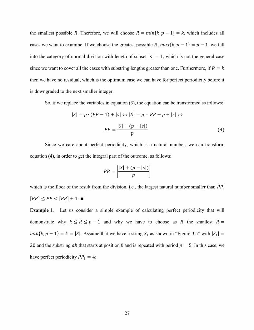
Example 1. Let us consider a simple example of calculating perfect periodicity that will

demonstrate why 𝑘 ≤ 𝑅 ≤ 𝑝 − 1 and why we have to choose as 𝑅 the smallest 𝑅 =

𝑚𝑖𝑛{𝑘, 𝑝 − 1} = 𝑘 = |𝑆|. Assume that we have a string 𝑆1 as shown in “Figure 3.a” with |𝑆1| =

20 and the substring 𝑎𝑏 that starts at position 0 and is repeated with period 𝑝 = 5. In this case, we

have perfect periodicity 𝑃𝑃1 = 4:

28

Figure 3 Different sequences for the calculation of perfect periodicity

𝑃𝑃1 = ⌊|𝑆1| + (𝑝 − |𝑠|)

𝑝⌋ = ⌊

20 + (5 − 2)

5⌋ ⇔

𝑃𝑃1 = ⌊23

5⌋ = ⌊4.6⌋ = 4

Suppose that we truncate the string to have |𝑆2| = 17 “Figure 3.b”. Then we have again

perfect periodicity 𝑃𝑃2 = 4:

𝑃𝑃2 = ⌊|𝑆2| + (𝑝 − |𝑠|)

𝑝⌋ = ⌊

17 + (5 − 2)

5⌋ ⇔

𝑃𝑃2 = ⌊20

5⌋ = ⌊4⌋ = 4.

29

We have to remember that perfect periodicity is not just the quotient but it is the quotient

incremented by 1, since 𝑃𝑃 = 𝑞 + 1. So, if we do the division and express the perfect periodicity

as the quotient plus 1 then we will have the following analysis

17/5 = 5 ∙ 3 + 2 ⇒ 𝑃𝑃 = 𝑞 + 1 = 3 + 1 = 4

and, moreover, we have no other values after the subset since the remainder of the division 17/5 is

2 = 𝑘, which is the length of the substring |𝑠| = 𝑘. As we have proved, this is the smallest value

the residual 𝑟 could take since 𝑘 ≤ 𝑅 ≤ 𝑝 − 1, 𝑘 > 0.

If we truncate the sequence by one more element to have |𝑆3| = 16 “Figure 3.c”, then the

perfect periodicity will be 𝑃𝑃3 = 3:

𝑃𝑃3 = ⌊|𝑆3| + (𝑝 − |𝑆|)

𝑝⌋ = ⌊

16 + (5 − 2)

5⌋ ⇔

𝑃𝑃3 = ⌊19

5⌋ = ⌊3.8⌋ = 3

instead of 4, because one character of the subset will be outside of the boundaries of the string 𝑆3.

Now we will have four remaining values (including 𝑎 at position 15, which is not an occurrence

anymore), which is actually the largest value the residual 𝑅 could take since 𝑘 ≤ 𝑅 ≤ 𝑝 − 1, 𝑘 >

0 and in this case 𝑝 − 1 = 5 − 1 = 4, while the remainder of the division 16/5 is 1 < 𝑘. Therefore,

we conclude that the optimum case for the perfect periodicity, before we fall into smaller number,

is when we have no remaining elements as in the second case in which 𝑅 = 𝑘 = |𝑠|.⧠

Lemma 1. (Perfect Periodicity starting at a position greater than 0) Consider a sequence

𝑇 = {𝑒0𝑒1…𝑒𝑛−1} of 𝑛 ∈ 𝑁∗elements and length |𝑇| = 𝑛 and a subset 𝑆 = {𝑒𝑖𝑒𝑖+1…𝑒𝑖+𝑘−1} of

the sequence 𝑇 of 𝑘 ∈ 𝑁∗ elements and length |𝑆| = 𝑘, where 0 ≤ 𝑖 < 𝑖 + 𝑘 − 1 ≤ 𝑛 − 1. If we

want to calculate perfect periodicity for the subset 𝑆 from the position of the first occurrence 𝑒𝑖,

30

where 𝑖 = 𝑆𝑡𝑎𝑟𝑡𝑖𝑛𝑔𝑃𝑜𝑠𝑖𝑡𝑖𝑜𝑛, then the perfect periodicity 𝑃𝑃 of the subset 𝑆, with period 𝑝 ∈

𝑁, 𝑝 ≥ 1, can be derived from the formula:

𝑃𝑃 = [(|𝑇| − 𝑖) + (𝑝 − |𝑆|)

𝑝]

Proof:

If we truncate sequence 𝑇 for 𝑖 elements from the beginning then we have a new sequence

𝑇1 with length:

|𝑇1| = |𝑇| − 𝑆𝑡𝑎𝑟𝑡𝑖𝑛𝑔𝑃𝑜𝑠𝑖𝑡𝑖𝑜𝑛 = |𝑇| − 𝑖

which it will give as result the formula of the Lemma 1 for the perfect periodicity if we change the

new value of |𝑇1| with its equivalent in the formula of Theorem 1:

𝑃𝑃 = [|𝑇1| + (𝑝 − |𝑆|)

𝑝]|𝑇1|=|𝑇|−𝑖⇔

𝑃𝑃 = [(|𝑇| − 𝑖) + (𝑝 − |𝑆|)

𝑝]

and we get the formula of the Lemma 1. ⧠

Figure 4 Original sequence for the calculation of perfect periodicity using Theorem 1

Figure 5 Transformed sequence for the calculation of perfect periodicity using Lemma 1

31

Example 2. Let us examine again the first case of Example 1 by calculating perfect periodicity

from a different starting element than 𝑒0 at position 0. We have the sequence as shown in “Figure

4” where we have calculated the perfect periodicity as 𝑃𝑃 = 4. However, assuming that we want

to calculate the perfect periodicity starting from the position 𝑖 = 4, as it is illustrated in “Figure 5”,

we will have:

𝑃𝑃 = [(|𝑇| − 𝑖) + (𝑝 − |𝑆|)

𝑝] = [

(20 − 4) + (5 − 2)

5] ⇔

𝑃𝑃 = [19

5] = [3.8] = 3

and we get the expected result because starting from position 4 we have excluded the first

occurrence of the subset and we have four free cells, one at the beginning and three at the end;

these are the most we can have, i.e., 1 + 3 = 4 = 𝑝 − 1. It is like creating a new sequence 𝑇1with

|𝑇1| = |𝑇| − 4 = 16, in which the subset starts from position 4 of the first sequence 𝑇 (position 0

of the new sequence 𝑇1) with four remaining elements at the end, including a at position 19, which

is not an occurrence any more as it is represented in “Figure 5”. ⧠

Lemma 2. (Perfect Periodicity starting at a position greater than 0 and ending at a

position less than n-1) Consider a sequence 𝑇 = {𝑒0𝑒1…𝑒𝑛−1} of 𝑛 ∈ 𝑁∗ elements and length

|𝑇| = 𝑛 and a subset 𝑆 = {𝑒𝑖𝑒𝑖+1…𝑒𝑖+𝑘−1} of the sequence 𝑇 of 𝑘 ∈ 𝑁∗ elements and length |𝑆| =

𝑘, where 0 ≤ 𝑖 < 𝑖 + 𝑘 − 1 ≤ 𝑛 − 1. If we want to calculate the perfect periodicity for the subset

𝑆 from the position of the first occurrence 𝑒𝑖, where 𝑖 = 𝑆𝑡𝑎𝑟𝑡𝑖𝑛𝑔𝑃𝑜𝑠𝑖𝑡𝑖𝑜𝑛, till another position

𝑒𝑚, where 𝑚 = 𝐸𝑛𝑑𝑖𝑛𝑔𝑃𝑜𝑠𝑖𝑡𝑖𝑜𝑛. Moreover, we have 0 ≤ i < 𝑖 + 𝑘 − 1 < 𝑚 ≤ 𝑛 − 1, which

means the perfect periodicity 𝑃𝑃 of the subset 𝑆, with period 𝑝 ∈ 𝑁, 𝑝 ≥ 1, can be derived from

the formula:

32

𝑃𝑃 = [(|𝑇| − 𝑖 − (|𝑇| − (𝑚 + 1))) + (𝑝 − |𝑆|)

𝑝] ⇔

𝑃𝑃 = [(𝑚 + 1 − 𝑖) + (𝑝 − |𝑆|)

𝑝]

Proof:

If we truncate sequence 𝑇 for 𝑖 elements from the beginning and (|𝑇| − (𝑚 + 1)) elements

from the end, to a new sequence 𝑇1 with length

|𝑇1| = |𝑇| − 𝑆𝑡𝑎𝑟𝑡𝑖𝑛𝑔𝑃𝑜𝑠𝑖𝑡𝑖𝑜𝑛 − (|𝑇| − (𝐸𝑛𝑑𝑖𝑛𝑔𝑃𝑜𝑠𝑖𝑡𝑖𝑜𝑛 + 1)) ⇔

|𝑇1| = |𝑇| − 𝑖 − (|𝑇| − (𝑚 + 1)) = 𝑚 + 1 − 𝑖

which it will give as result the formula of Lemma 2 for the perfect periodicity if we change the new

value of |𝑇1| with its equivalent in the formula of Theorem 1:

𝑃𝑃 = [|𝑇1| + (𝑝 − |𝑆|)

𝑝]|𝑇1|=𝑚+1−𝑖⇔

𝑃𝑃 = [(𝑚 + 1 − 𝑖) + (𝑝 − |𝑆|)

𝑝]

and we obtain the formula of Lemma 2. ⧠

In the second lemma we get the general formula that represents the perfect periodicity of a

subset in a time series because if we set 𝑚 + 1 = |𝑇| and 𝑖 = 0 we fall in the formula of Theorem

1, while with 𝑚 + 1 = |𝑇| and 𝑖 ≠ 0 we fall in the formula of the first lemma in which we start

from a position different than 0.

Example 3. Let us use again Example 2 to calculate perfect periodicity from element 𝑒𝑖 at

position 𝑖 = 4 but for a different ending element 𝑒𝑚 at position 𝑚 = 14. Then we will have as

shown in “Figure 6” a new sequence 𝑇1 starting at position 4 and ending at position 14 of the original

sequence, in which perfect periodicity will be:

33

Figure 6 Sequence for calculation of perfect periodicity using Lemma 2

𝑃𝑃 = [(|𝑇| − 𝑖 − ((|𝑇| − 1) − 𝑚)) + (𝑝 − |𝑆|)

𝑝] ⇔

𝑃𝑃 = [(𝑚 + 1 − 𝑖) + (𝑝 − |𝑆|)

𝑝] ⇔

𝑃𝑃 = [(14 + 1 − 4) + (5 − 2)

5] = [

14

5] = [2.8] = 2

and we get the expected result because starting from position 4 and ending at position 14 of the

original sequence, we can have only two occurrences of the subset with four remaining elements

at the end, including a at position 14 of the original sequence or position 10 of the new sequence,

which is not an occurrence anymore. ⧠

Definition 2. (Partial Perfect Periodicity) Consider a string 𝑆 = {𝑒0𝑒1…𝑒𝑛−1} of 𝑛 ∈

𝑁∗elements and length |𝑆| = 𝑛 and a substring 𝑠 = {𝑒𝑖𝑒𝑖+1…𝑒𝑖+𝑘−1}, of the string 𝑆, of 𝑘 ∈ 𝑁∗

elements and length |𝑠| = 𝑘 that occurs starting at position 𝑖 where 0 ≤ 𝑖 ≤ 𝑖 + 𝑘 − 1 ≤ 𝑛 − 1.

We define as Partial Perfect Periodicity 𝑃𝑃𝑃(𝑗, 𝑗 + 𝑙) of the substring 𝑠 in an area 𝑆′ of string 𝑆

starting at position 𝑗 and ending at position 𝑗 + 𝑙, with 0 ≤ 𝑗 ≤ 𝑗 + 𝑙 ≤ 𝑛 − 1 and period 𝑝 ∈

𝑁, 𝑝 ≥ 1, the maximum number of repetitions that 𝑠 can have with period 𝑝 in the continuous area

𝑆′ of string 𝑆 without overlapping, where 𝑆′ = {𝑒𝑗𝑒𝑗+1…𝑒𝑗+𝑙} and 0 ≤ 𝑗 ≤ 𝑖 ≤ 𝑖 + 𝑘 − 1 ≤ 𝑗 +

𝑙 ≤ 𝑛 − 1.

34

Definition 3. (Full Confidence) Consider a string 𝑆 = {𝑒0𝑒1…𝑒𝑛−1} of 𝑛 ∈ 𝑁∗elements and


|𝑠| = 𝑘 that occurs starting at position 𝑖 where 0 ≤ 𝑖 ≤ 𝑖 + 𝑘 − 1 ≤ 𝑛 − 1. We define as Full

Confidence FC of the substring s, with period 𝑝 ∈ 𝑁, 𝑝 ≥ 1, the ratio of the successful occurrences

of substring s in string S over the Perfect Periodicity PP of the substring s:

𝐹𝐶 =𝑆𝑢𝑐𝑐𝑒𝑠𝑓𝑢𝑙 𝑂𝑐𝑐𝑢𝑟𝑟𝑒𝑛𝑐𝑒𝑠

𝑃𝑒𝑟𝑓𝑒𝑐𝑡 𝑃𝑒𝑟𝑖𝑜𝑑𝑖𝑐𝑖𝑡𝑦

By successful occurrences of substring s, we define all occurrences of 𝑠 at positions defined by the

starting position of 𝑠 and the period p.

Definition 4. (Partial Confidence) Consider a string 𝑆 = {𝑒0𝑒1…𝑒𝑛−1} of 𝑛 ∈ 𝑁∗elements and


|𝑠| = 𝑘 that occurs starting at position 𝑖 where 0 ≤ 𝑖 ≤ 𝑖 + 𝑘 − 1 ≤ 𝑛 − 1. We define as Partial

Confidence PC of the substring s, with period 𝑝 ∈ 𝑁, 𝑝 ≥ 1, the ratio of the successful occurrences

of substring s in string S over the Partial Perfect Periodicity 𝑃𝑃𝑃(𝑗, 𝑗 + 𝑙) of the substring s:

𝑃𝐶 =𝑆𝑢𝑐𝑐𝑒𝑠𝑓𝑢𝑙 𝑂𝑐𝑐𝑢𝑟𝑟𝑒𝑛𝑐𝑒𝑠

𝑃𝑎𝑟𝑡𝑖𝑎𝑙 𝑃𝑒𝑟𝑓𝑒𝑐𝑡 𝑃𝑒𝑟𝑖𝑜𝑑𝑖𝑐𝑖𝑡𝑦

By successful occurrences of substring s, we define all occurrences of 𝑠 in the area (𝑗, 𝑗 + 𝑙) of S

defined by the starting position 𝑗, ending position 𝑗 + 𝑙 and the period p.

3.3 Full and Reduced Suffix Array

Before continuing the discussion, we need to introduce two new definitions for the suffix

array data structure. These definitions will differentiate the new version of the suffix array from

the original data structure as introduced by Manber and Myers [Manber and Myers 90]. Here it

can be claimed that the new definition is actually a new data structure more powerful and flexible

35

than the traditional suffix array, though they share some characteristics [Xylogiannopoulos et al.

16b].

Definition 5. (Full Suffix Array) We define as Full Suffix Array of a string 𝑆, constructed from

a finite alphabet 𝛴, the array of the actual lexicographically sorted suffix strings of the string. The

full suffix array has one column for the index of the position where each suffix string occurs in the

string and another column for the actual full suffix strings “Figure 7.b”.

Definition 6. (Reduced Suffix Array) We define as Reduced Suffix Array of width 𝑙 of a string

𝑆, constructed from a finite alphabet 𝛴, the array of the actual lexicographically sorted suffix

strings such that their lengths have been upper-bounded to any length 𝑙 less than the original length

of the string such that 1 ≤ 𝑙 < |𝑆| = 𝑛, where with |𝑆| = 𝑛 we define the cardinality (length) of

the string. Any suffix string with length larger than the upper bound is truncated (at the end) to a

length equal to the upper bound. The reduced suffix array has one column for the index of the

position where each suffix string occurs in the string and another column for the reduced suffix

strings “Figure 7.c”.

Figure 7 The suffix strings of the string kananaskis, the full suffix array and the reduced

suffix array of width 𝑙 = 5 < 10 = 𝑛

36

3.3.1 Maximum Space Required Capacity Theorem

Theorem 2. (Maximum Space Required Capacity of the Reduced Suffix Array) Consider a

string 𝑆 of size 𝑛 and let 𝐴 be its equivalent suffix array of size 𝑛×𝑛 with 𝑛(𝑛+1)

2 elements. The

size of a suffix array 𝐵 required to include all string periodicities that 𝑆 can have is 𝑛×𝑛

2 and the

number of elements of suffix array 𝐵 is:

‖𝐵‖ =3

4∙𝑛(𝑛 + 1)

2−𝑛

8≅3

4‖𝐴‖

Proof:

From Gauss formula for the summation of 𝑛 integers we know that ∑ 𝑘𝑛1 =𝑛∙(𝑛+1)

2. From

Theorem 1, we know that perfect periodicity is 𝑃𝑃 =|𝑇|+𝑝−|𝑆|

𝑝. In order for the formula to be

meaningful, 𝑃𝑃 should be at least 2, otherwise, if it is 1 we do not have periodicity (in such a case

we can have only a sequence of a single digit repeating itself in the sequence e.g., aaaa…a). So, if

we solve the equation for 𝑃𝑃 = 2 we get:

2 =𝑛 + 𝑝 − |𝑆|

𝑝⇔ 2 ∗ 𝑝 = 𝑛 + 𝑝 − |𝑆|⇔ 𝑝 + |𝑆| = 𝑛

The maximum values that both variables 𝑝 and 𝑆 can have simultaneously are 𝑝 = |𝑆| =

𝑛

2. So, the longest pattern we can have in a sequence in order to have at least periodicity 2 with

period 𝑝 =𝑛

2 is |𝑆| =

𝑛

2 , or |𝑆| = [

𝑛

2] in order to cover cases where the length of sequence 𝑇 is

odd.

So, the actual suffix array size that we have to store in order to search for periodicities is:

‖𝐵‖ =𝑛(𝑛 + 1)

2−

𝑛2 (𝑛2 + 1)

2⇔

37

‖𝐵‖ =𝑛(𝑛 + 1)

2−4

4∙

𝑛2 (𝑛2 + 1)

2⇔

‖𝐵‖ =𝑛(𝑛 + 1)

2−1

4∙𝑛(𝑛 + 2)

2⇔

‖𝐵‖ =𝑛(𝑛 + 1)

2−1

4∙𝑛(𝑛 + 1) + 𝑛

2⇔

‖𝐵‖ =𝑛(𝑛 + 1)

2−1

4∙𝑛(𝑛 + 1)

2−𝑛

8⇔

‖𝐵‖ =3

4∙𝑛(𝑛 + 1)

2−𝑛

8⇒

‖𝐵‖ ≅3

4∙𝑛(𝑛 + 1)

2=3

4‖𝐴‖

We can eliminate the factor 𝑛

8 , since it is very small compared to

3

4∙𝑛(𝑛+1)

2, to get the final

result of ¾ of the elements in the original suffix array 𝐴 without harming the general rule of the

proximity we have used to describe suffix array 𝐵. ∎

Figure 8 The suffix array of string kananaskis and the part that does not need to be stored

38

3.4 Longest Expected Repeated Pattern (LERP)

Definition 7. (Pattern) Given a finite alphabet 𝛴, we define as Pattern any ordered, finite,

sequence of characters from the alphabet 𝛴.

Definition 8. (Repeated Pattern) Given a string S constructed from a finite alphabet 𝛴, we define

a substring 𝑠 of S as Repeated Pattern if it occurs at least twice in S.

Definition 9. (Longest Expected Repeated Pattern) Given a string S constructed from a finite

alphabet 𝛴, we define as Longest Expected Repeated Pattern (LERP) the longest periodic substring

𝑠 of 𝑆.

LERP always satisfies the following:

1 ≤ 𝐿𝐸𝑅𝑃 ≤𝑛

2

where 𝑛 is the length of the sequence; this upper bound is required since if it was larger than 𝑛

2 then

the specific pattern would not repeat in the sequence. Although definition requires periodicity this

does not limit LERP only to periodic patterns because any pattern occurring twice is periodic.

Periodicity is important at this stage to avoid overlapping patterns with length greater than 𝑛/2.

The definition can be expanded for overlapping patterns or patterns occurring more than twice,

yet, for the next theorems it will be used as it is and it will be generalized later during the proof of

the Probabilistic Existence of Longest Expected Repeated Pattern Theorem (Theorem 4).

3.4.1 Reduced Suffix Array Maximum Space Required Capacity Theorem and Related

Lemmas

Theorem 3. (Reduced Suffix Array Maximum Space Required Capacity) Consider a string

𝑆 of size 𝑛 and let 𝐴 be its equivalent full suffix array of size 𝑛×𝑛 and 𝑛(𝑛+1)

2 elements. Let 𝐵 be

the reduced suffix array of dimension 𝑛×𝑙, where 𝑙 ≪ 𝑛, in order to have all string periodicities

39

that 𝑆 can have with longest expecting repeated pattern length 𝑙. The number of elements of the

suffix array 𝐵 is:

‖𝐵‖ = 𝑛𝑙 −(𝑙 − 1)𝑙

2≅ 2

𝑙

𝑛‖𝐴‖

Proof:

Since we need to have substrings with length no more than 𝑙 elements then from the full

suffix array 𝐴 we can exclude the part of all substrings that are longer than 𝑙. If we start counting

from the bottom of the suffix array “Figure 9.a”, we will observe that we have 𝑙 − 1 substrings

with length less than 𝑙, one with length exactly 𝑙 and 𝑛 − 𝑙 with length greater than 𝑙. So, we have

(𝑙−1)𝑙

2 elements for the substrings with length less than 𝑙 and 𝑙 + (𝑛 − 𝑙)𝑙 = (𝑛 − 𝑙 + 1)𝑙 elements

for the substring with length greater than or equal to 𝑙. The elements of the suffix array 𝐴 that we

have to exclude are (𝑛−𝑙)(𝑛−𝑙)

2 “Figure 9.a”. The elements of the reduced suffix array 𝐵 will be:

‖𝐵‖ = (𝑛 − 𝑙 + 1)𝑙 +(𝑙 − 1)𝑙

2⇔

‖𝐵‖ = 𝑛𝑙 − (𝑙 − 1)𝑙 +(𝑙 − 1)𝑙

2⇔

‖𝐵‖ = 𝑛𝑙 −(𝑙 − 1)𝑙

2 (5)

We can assume the following without significant error that harms the general rule of the

proximity:

(𝑙 − 1)𝑙

2≅𝑙2

2 (6)

So, we can transform equation (5) based on expression (6) as follows:

‖𝐵‖ ≅ 𝑛𝑙 −𝑙2

2= 𝑙 (𝑛 −

𝑙

2) ⇒

40

‖𝐵‖ ≅𝑛

𝑛𝑙 (𝑛 −

𝑙

2) =

𝑙

𝑛(𝑛 (𝑛 −

𝑙

2)) ⇒

‖𝐵‖ ≅2

2∙𝑙

𝑛(𝑛 (𝑛 −

𝑙

2)) = 2

𝑙

𝑛(𝑛 (𝑛 −

𝑙2)

2) (7)

Because 𝑙 ≪ 𝑛, we can assume again without significant error that hurts the general rule

of the proximity that 𝑛 −𝑙

2≅ 𝑛 ≅ 𝑛 + 1. So, expression (7) will be transformed as follows:

‖𝐵‖ ≅ 2𝑙

𝑛(𝑛(𝑛 + 1)

2) = 2

𝑙

𝑛‖𝐴‖

So, we have shown that for large 𝑛 and 𝑙 ≪ 𝑛, the following expression

‖𝐵‖ ≅ 2𝑙

𝑛‖𝐴‖ (8)

is satisfied with great proximity. ∎

Figure 9 The suffix strings of string kananaskis and the Full/Reduced Suffix Array with

substrings of length at most three

41

Because of the theorem and the concluded formula, the space required capacity of the

reduced suffix array will be linear since 2𝑙 can be considered a constant comparing to 𝑛.

Lemma 3. (LERP Reduced Suffix Array Linear Space Required Capacity) Consider a

string 𝑆 of size 𝑛, and let 𝐴 be its equivalent full suffix array of size 𝑛×𝑛 of 𝑛(𝑛+1)

2 elements and

required space capacity 𝑂(𝑛2). Let 𝐵 be the reduced suffix array of dimension 𝑛×𝑙, where 𝑙 ≪ 𝑛,

and number of elements ‖𝐵‖ ≅ 2𝑙

𝑛‖𝐴‖, in order to have all string periodicities that 𝑆 can have

with longest expecting repeated pattern length 𝑙. Then the required space capacity of the suffix array

𝐵 is linear and it is 𝑂(𝑛1+

𝑥

𝑦) where 𝑥, 𝑦 are the indexes of the powers of 10 that represent 𝑙 and 𝑛,

respectively, (𝑙 = 10𝑥 , 𝑛 = 10𝑦).

Proof:

It is known from Gauss formula that the suffix array 𝐴 has ‖𝐴‖ =𝑛(𝑛+1)

2 elements and,

therefore, has 𝑂(𝑛2) required space capacity. We have also proven that for the suffix array 𝐵 the

number of elements is ‖𝐵‖ ≅ 2𝑙

𝑛‖𝐴‖, where 𝑙 ≪ 𝑛, with great proximity.

However, we can observe that we can transform the formula of Theorem 3 as follows:

‖𝐵‖ ≅ 2𝑙

𝑛‖𝐴‖ = 2

𝑙

𝑛∙𝑛(𝑛 + 1)

2= 𝑙(𝑛 + 1) ⇒

‖𝐵‖ ≅ 𝑙𝑛 (9)

If we write 𝑙 and 𝑛 as powers of ten then we will have:

𝑙 = 10𝑥 (10)

and

𝑛 = 10𝑦 (11)

where 𝑥, 𝑦 ∈ 𝑅+∗ . Then equations (10) and (11) can be transformed as follows:

42

𝑙 = 10𝑥 ⇔ 𝑙𝑜𝑔 𝑙 = 𝑙𝑜𝑔 10𝑥 ⇔ 𝑙𝑜𝑔 𝑙 = 𝑥 (12)

and

𝑛 = 10𝑦 ⇔ 𝑙𝑜𝑔 𝑛 = 𝑙𝑜𝑔 10𝑦 ⇔ 𝑙𝑜𝑔 𝑛 = 𝑦 (13)

If we divide equation (12) with (13) we will get:

𝑙𝑜𝑔 𝑙

𝑙𝑜𝑔 𝑛=𝑥

𝑦⇔ 𝑙𝑜𝑔 𝑙 =

𝑥

𝑦𝑙𝑜𝑔 𝑛 = 𝑙𝑜𝑔 𝑛

𝑥𝑦 ⇔ 𝑙 = 𝑛

𝑥𝑦 (14)

and expression (9) can be transformed as follows:

‖𝐵‖ ≅ 𝑛𝑥𝑦𝑛 = 𝑛

1+𝑥𝑦 (15)

and the required space capacity of the suffix array B will be close to linear 𝑂(𝑛1+

𝑥

𝑦). ⧠

Example 4. If we have 𝑙 = 10 and 𝑛 = 109 then 𝑥 = 1 and 𝑦 = 9. From the previous lemma,

we will have the following:


1+𝑥𝑦 = 𝑛1+

19 = 𝑛1.11111

and 𝑛1.111 = 9,999,769,744 which is close to 10 ∗ 109 and to 𝑛, while 𝑛2 = 1018.

Moreover, if we have 𝑙 = 10 and 𝑛 = 101000 then 𝑥 = 1 and 𝑦 = 1,000. From the

previous lemma, we will have that:


1+𝑥𝑦 = 𝑛

1+1

1,000 = 𝑛1.001

and 𝑛1.001 ≅ 101,000, while 𝑛2 = 101,000,000. ⧠

3.5 Probabilistic Existence of Longest Expected Repeated Pattern Theorem and Related

Lemmas

So far it has been proven in Theorem 3 that if we select a number 𝑙 ≪ 𝑛 as the maximum

length of all strings that occur at least twice in a string then the total space capacity of the suffix

array is linear. However, we have to examine if it is logical to expect such a small value for 𝑙 when

43

we have a very large string. “Extraordinary” strings where LERP cannot be applied will exist and

since it is impossible to examine all strings in order to extract a general rule, we have to check the

probability of the existence of LERP. In order to prove that, the following theorem of the

probabilistic existence of the longest expected repeated pattern is introduced.

In the following theorem, we use the notions “considerably long and random” for the string

and “reasonably long” for the repeated pattern. The randomness has been thoroughly described in

Chapter 2 and in the following paragraphs we will clarify what we mean by “considerably” and

“reasonably long” from a mathematical perspective. According to the Law of Large Numbers

Theorem while conducting the same experiment many times the average of the results should be

very close to the expected value. This means that according to the examples described in Chapter 2

if we flip a coin ten times we can have heads seven times (70%) and tails three time (30%) while if

we flip the same coin one thousand times we will have frequencies very close to 50% for both heads

and tails. Assuming that we create a string from the results based on the alphabet {0, 1} (heads/tails),

the string created, in order to produce the expected results and present randomness, should be

“considerably long” according to the Law of Large Numbers Theorem. The “considerably long”

string notion cannot be uniquely and precisely defined because it depends on other factors than just

the number of repetitions, such as the size of the alphabet. For example, in the case of a coin the

alphabet has size 2 and maybe one thousand repetitions are enough for very good results since we

expect approximately 500 occurrences for each digit and the deviation (error) from the central value

will be small, e.g., occurrences of 490 and 510 for each one is just 2% deviation (error). In case of

the English language alphabet of 26 characters a similar string of one thousand characters cannot

give satisfactory results according the Law of Large Numbers Theorem since we expect

44

approximately 38 occurrences per character and the deviation from the central value (error) will be

significantly larger, e.g., an occurrence of 31 instead of 38 means 20% deviation (error).

The notion of the “reasonably long” repeated pattern notion is derived by the Normal

Numbers definition as presented in Chapter 2 and defined by Calude in [Calude 95]. Depending

on the length of a string we expect to have arrangements of the letters of the alphabet up to a

specific length which will occur with a specific frequency. Again the “reasonably long” notion

here cannot be defined uniquely and precisely for every case since it is directly dependent on the

length of the string and the size of the alphabet. For example, in the first 100 digits of π decimal

expansion, all decimal digits occur with approximately 10% frequency and most of the two digits

arrangements occur with 1% frequency. However, there are only three occurrences of

arrangements of length 3 digits (“592”, “628” and “862”), which appear only twice, and no other

kind of longer digits’ arrangements (four and more).

Theorem 4. (Probabilistic Existence of Longest Expected Repeated Pattern) Let 𝑆 be a

string of size 𝑛 constructed from a finite alphabet 𝛴 of size 𝑚 ≥ 2 and let 𝑠 be a substring (of 𝑆) of

length 𝑙. Let 𝑋 be the event that “substring 𝑠 occurs at least twice in string 𝑆.” If 𝑆 is considerably

long and random, and 𝑠 is reasonably long then the probability 𝑃(𝑋) of the event 𝑋 is extremely

small. An upper bound for the probability 𝑃(𝑋) is directly proportional to the square of the length

of string 𝑆 and inversely proportional to the size of the alphabet 𝑚 raised to the power of the length

of substring 𝑠:

𝑃(𝑋) =(𝑛 − 2𝑙 + 1)(𝑛 − 2𝑙 + 2)

2𝑚𝑙<𝑛2

2𝑚𝑙

or

𝑃(𝑋) =𝑛2

2𝑚𝑙 (16)

45

where the over-bar is used to define an upper bound of the underlying value.

Proof:

The first step in the proof is the calculation of the discrete sample space of the experiment,

𝛺 = {𝜔1, 𝜔2, … , 𝜔𝑘} where 𝜔 defines a string and 𝑘 is the total number of simple events. It is

possible to rewrite the same expression as:

𝛺 = {𝜔:𝜔 𝑠𝑖𝑚𝑝𝑙𝑒 𝑒𝑣𝑒𝑛𝑡 𝑜𝑓 𝑡ℎ𝑒 𝑒𝑥𝑝𝑒𝑟𝑖𝑚𝑒𝑛𝑡}

We define as discrete sample space 𝛺(𝑆) the set of all strings we can have of length |𝑆| =

𝑛, constructed from an alphabet 𝛴 of 𝑚 letters. In the problem we examine, we care about the

arrangements with repetition of the 𝑚 letters of the alphabet in the 𝑛 length string, which is the

ordering of 𝑖 elements selected from 𝑘 different ones where any of the elements can be selected

randomly many times. Their number is:

𝑉𝑘(𝑖)= 𝑘𝑖

or in the case we examine:

|𝛺(𝑆)| = 𝑉𝑚(𝑛)= 𝑚𝑛

The size of the discrete sample space 𝛺(𝑆) gives all the possible strings of length 𝑛, which

may be constructed from an alphabet 𝛴 of 𝑚 letters. If all strings have the same probability to occur

in the experiment then the probability of a specific string 𝑆i ∈ 𝛺(𝑆), which we want to examine, to

occur is exactly one out of |𝛺(𝑆)| or:

𝑃(𝑆𝑖) =1

|𝛺(𝑆)|

Note that in order for all strings to have the same probability to occur as mentioned, each

string that belongs to the discrete sample space 𝛺(𝑆) has to be random, as the theorem requires. To

prove the Theorem, we need to calculate all possible simple events expressed as:

46

Figure 10 Possible occurrences of string ab in a 5 character long string

Figure 11 Possible occurrences of string ba in 5 character long string

𝑋: 𝑎 𝑠𝑢𝑏𝑠𝑡𝑟𝑖𝑛𝑔 𝑠 𝑜𝑓 𝑙𝑒𝑛𝑔𝑡ℎ 𝑙 𝑜𝑐𝑐𝑢𝑟𝑠 𝑎𝑡 𝑙𝑒𝑎𝑠𝑡 𝑡𝑤𝑖𝑐𝑒

Then the probability of event X to occur will be:

𝑃(𝑋) =𝑁𝑋|𝛺(𝑆)|

where 𝑁𝑋 = 𝑡ℎ𝑒 𝑛𝑢𝑚𝑏𝑒𝑟 𝑜𝑓 𝑎𝑙𝑙 𝑓𝑎𝑣𝑜𝑟𝑎𝑏𝑙𝑒 𝑠𝑖𝑚𝑝𝑙𝑒 𝑒𝑣𝑒𝑛𝑡𝑠.

Assume we have a string 𝑆 of length 𝑛 = 5 constructed by an alphabet 𝛴 of 3 letters {a, b,

c}. We want to calculate the probability of all substrings with length 2 occur at least twice in the

string.

The discrete sample space 𝛺(𝑆) of the experiment has a population of:

|𝛺(𝑆)| = 𝑉𝑚(𝑛)= 𝑚𝑛 = 35 = 243

The outcome 243 defines actually the total number of possible strings 𝑆 of length 5

constructed from an alphabet of any 3 letters that can exist.

In order to calculate the probability of event X we have to find out all strings of length 5 that

can be constructed by the three letters {a, b, c} and include at least twice all substrings of type {**}.

First of all, let us start with the strings of length 5 that have substring ab (event 𝑋1) at position 1,

47

therefore, the substring occupies cells 1 and 2; see “Figure 10.a”. In this case, the substring ab can

occur again at positions 3 “Figure 10.a” and 4 “Figure 10.b”. In case of “Figure 10.a” we have three

strings that can exist with the substring at positions 1 and 3 which are of type {abab*} where the

star ‘*’ represents any of the three letters of the alphabet. Therefore, we have the following possible

strings: (1) {ababa}, (2) {ababb} and (3) {ababc}. In case of “Figure 10.b” we can have three

strings of type {ab*ab}. Therefore, we have the following strings: (4) {abaab}, (5) {abbab} and

(6) {abcab} and we have found all possible strings with ab at position 1, in which the substring ab

occurs at least twice. We further proceed with the substring to appear at position 2. In this case, in

“Figure 10.c” the substring ab can occur again at position 4. For this case, we have three possible

strings of type {*abab}. Therefore, we have the following three strings: (7) {aabab}, (8) {babab}

and (9) {cabab}. These nine strings are all possible strings (favorable simple events) of length 5

constructed from the alphabet {a,b,c} that includes at least twice the substring ab.

The probability of the substring ab to occur at least twice in string S is the fraction of the

favorable events over the total events or the population of the discrete sample space as we have

described so far. Therefore, the probability will be:

𝑃(𝑋1) =𝑁𝑋1|𝛺(𝑆)|

=9

243

The total arrangements with repetitions for the pairs we can construct from the three letters

of the alphabet are:

𝑉3(2)= 32 = 9

More specifically, the substrings of length 2 are {𝑎𝑎, 𝑎𝑏, 𝑎𝑐, 𝑏𝑎, 𝑏𝑏, 𝑏𝑐, 𝑐𝑎, 𝑐𝑏, 𝑐𝑐}. From

the addition principle, we can calculate the probability, or more precisely an upper bound for the

probability, of the outcome X as the addition of the probability of all the nine events:

{𝑋𝑖: 𝑎 𝑠𝑢𝑏𝑠𝑡𝑟𝑖𝑛𝑔 𝑜𝑓 𝑡𝑦𝑝𝑒 {∗∗} 𝑜𝑐𝑐𝑢𝑟𝑠 𝑎𝑡 𝑙𝑒𝑎𝑠𝑡 𝑡𝑤𝑖𝑐𝑒}

48

where 1 ≤ 𝑖 ≤ 9:

𝑃(𝑋) =𝑁𝑋|𝛺(𝑇)|

=∑𝑃(𝑋𝑖)

9

𝑖=1

= 99

243=81

243 (17)

However, the probability calculated is not the actual one but just an upper bound of the

probability for event X. The actual probability is less than 81/243. Let us explain why this happens

by taking as an example the substring ba.

As with substring ab, we can have the strings of type: (i) {baba*}, (ii) {ba*ba} and (iii)

{*baba}, which will give us 9 possible strings as shown in “Figure 11”. However, what is very

important to notice is that string {babab} from “Figure 11.a” where ‘*’ is b and {ababa} from

“Figure 11.c” where ‘*’ is a, have been already counted when we calculated event 𝑋1 for substring

ab as shown in “Figure 10.c” and “Figure 10.a”, respectively. Therefore, we have to exclude them

when calculating the total favorable events of the substring ba. This process must be completed for

all the remaining double letter substrings. The final outcome will be that the total favorable events

in this case are 69 and not 81 as it was calculated in (17). Consequently, the actual probability with

exclusions will be:

𝑃(𝑋) =𝑁𝑋|𝛺(𝑆)|

=69

243

In order to calculate precisely the probability of the outcome X, we have to calculate not

only the favorable events of each double character substring, but also the exclusions in case of

repeated strings. This is very complex to be calculated and since we care only for an upper bound

for the probability, which gives us a higher probability than the actual, we are satisfied with the

calculation from the addition principle outcome (17).

Based on the above process we can generalize and create the formula summarizing the

whole process that has been described by implementing the following. First, when the substring

49

with length 𝑙 = 2 occurs at position 1, we have 2 possible occurrences (at positions 3 and 4). For

each of these occurrences we have 3 strings because we have only one cell free at positions 5 and

3, respectively. For this case, we have 2 ∙ 3 strings, or in general 2𝑚𝑛−2𝑙, where 𝑛 = 5 and 𝑚 = 2.

If the substring occurs at position 2 then we have only one possible occurrence (at position 4). For

this occurrence, we have only on free cell at position 1, and thus we have 1 ∙ 3 strings, or in general

1𝑚𝑛−2𝑙. These results can be added as follows:

∑ (𝑘𝑚𝑛−2𝑙)

𝑛−2𝑙+1

𝑘=1

(18)

where 𝑛 − 2𝑙 + 1 is the number of all possible positions in the string where the substring can occur,

which is the length of the string plus 1, minus double the length of the substring, since we want it

to occur twice.

From the Addition Principle in Probabilities, we will have that an upper bound for the

probability of the outcome X is based on (17):

𝑃(𝑋) =𝑚𝑙 ∑ (𝑘𝑚𝑛−2𝑙)𝑛−2𝑙+1

𝑘=1

𝑚𝑛⇔

𝑃(𝑋) =𝑚𝑙𝑚𝑛−2𝑙 ∑ 𝑘𝑛−2𝑙+1

𝑘=1

𝑚𝑛⇔

𝑃(𝑋) =𝑚𝑙𝑚𝑛−2𝑙

(𝑛 − 2𝑙 + 1)(𝑛 − 2𝑙 + 2)2

𝑚𝑛⇔

𝑃(𝑋) =𝑚𝑙𝑚𝑛−2𝑙(𝑛 − 2𝑙 + 1)(𝑛 − 2𝑙 + 2)

2𝑚𝑛⇔

𝑃(𝑋) =𝑚𝑛−𝑙(𝑛 − 2𝑙 + 1)(𝑛 − 2𝑙 + 2)

2𝑚𝑛⇔

𝑃(𝑋) =(𝑛 − 2𝑙 + 1)(𝑛 − 2𝑙 + 2)

2𝑚𝑙 (19)

Equation (19) can be further simplified as follows:

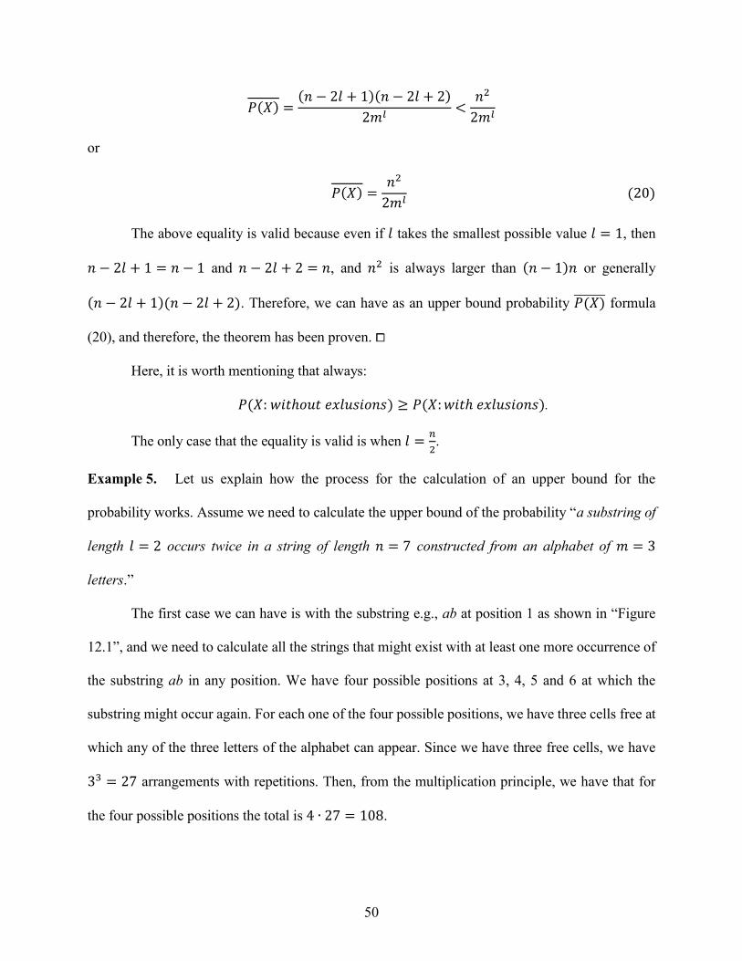
50

𝑃(𝑋) =(𝑛 − 2𝑙 + 1)(𝑛 − 2𝑙 + 2)

2𝑚𝑙<𝑛2

2𝑚𝑙

or

𝑃(𝑋) =𝑛2

2𝑚𝑙 (20)

The above equality is valid because even if 𝑙 takes the smallest possible value 𝑙 = 1, then

𝑛 − 2𝑙 + 1 = 𝑛 − 1 and 𝑛 − 2𝑙 + 2 = 𝑛, and 𝑛2 is always larger than (𝑛 − 1)𝑛 or generally

(𝑛 − 2𝑙 + 1)(𝑛 − 2𝑙 + 2). Therefore, we can have as an upper bound probability 𝑃(𝑋)̅̅ ̅̅ ̅̅ ̅ formula

(20), and therefore, the theorem has been proven. ⧠

Here, it is worth mentioning that always:

𝑃(𝑋: 𝑤𝑖𝑡ℎ𝑜𝑢𝑡 𝑒𝑥𝑙𝑢𝑠𝑖𝑜𝑛𝑠) ≥ 𝑃(𝑋:𝑤𝑖𝑡ℎ 𝑒𝑥𝑙𝑢𝑠𝑖𝑜𝑛𝑠).

The only case that the equality is valid is when 𝑙 =𝑛

2.

Example 5. Let us explain how the process for the calculation of an upper bound for the

probability works. Assume we need to calculate the upper bound of the probability “a substring of

length 𝑙 = 2 occurs twice in a string of length 𝑛 = 7 constructed from an alphabet of 𝑚 = 3

letters.”

The first case we can have is with the substring e.g., ab at position 1 as shown in “Figure

12.1”, and we need to calculate all the strings that might exist with at least one more occurrence of

the substring ab in any position. We have four possible positions at 3, 4, 5 and 6 at which the

substring might occur again. For each one of the four possible positions, we have three cells free at

which any of the three letters of the alphabet can appear. Since we have three free cells, we have

33 = 27 arrangements with repetitions. Then, from the multiplication principle, we have that for

the four possible positions the total is 4 ∙ 27 = 108.

51

In the second case shown in “Figure 12.2” where the substring occurs at position 2, we have

three possible positions where the substring might occur again at positions 4, 5 and 6. In each of

the three possible positions we have again three free cells at which any of the three letters of the

alphabet may appear. Therefore, we have 33 = 27 arrangements with repetitions and the total is

3 ∙ 27 = 81. Similarly, we calculate the total number of strings for case 3 (the first occurrence of

the substring is at position 3) as shown in “Figure 12.3” which is 2 ∙ 27 = 54; and for case 4 (the

first occurrence of the substring is at position 4) as shown in “Figure 12.4”, where the total number

of strings is 1 ∙ 27 = 27.

Therefore, the total favorable events for each substring of length 𝑙 = 2 is 108 + 81 + 54 +

27 = 270, while the discrete sample space is of size 37 = 2187. So, an upper bound for the

probability based on Theorem 4 will be:

𝑃(𝑋) =9 ∙ 270

2187

The aforementioned process identifies all possible second occurrences’ positions only at the

right of the first substring’s occurrence, since any possible occurrence at the left has already been

calculated in one of the previous steps, e.g., in case 3 we have **ab*** and we search for **abab*

as in “Figure 12.3”, while we can also have abab*** as in “Figure 12.1”, which has already been

calculated in case 1.

Figure 12 Possible occurrences of string ab in 7 characters long string

52

If we calculate the upper bound probability based on the above then we can try to reverse

the process in order to reach formula (16) of Theorem 4. We will have:

𝑃(𝑋) =9(1 ∙ 27 + 2 ∙ 27 + 3 ∙ 27 + 4 ∙ 27)

37⇔

𝑃(𝑋) =9 ∙ 27(1 + 2 + 3 + 4)

37⇔

𝑃(𝑋) =9 ∙ 27∑ 𝑘4

𝑘=1

37⇔

𝑃(𝑋) =𝑚2𝑚3∑ 𝑘4

𝑘=1

𝑚7⇔

𝑃(𝑋) =𝑚𝑙𝑚𝑛−2𝑙 ∑ 𝑘𝑛−2𝑙+1

𝑘=1

𝑚𝑛⇔

𝑃(𝑋) =𝑚𝑙𝑚𝑛−2𝑙

(𝑛 − 2𝑙 + 1)(𝑛 − 2𝑙 + 2)2

𝑚𝑛⇔

𝑃(𝑋) =(𝑛 − 2𝑙 + 1)(𝑛 − 2𝑙 + 2)

2𝑚𝑙

where 𝑛 = 7, 𝑚 = 3 and 𝑙 = 2; and this is the formula we have calculated in Theorem 4.

As it has been discussed, the upper bound for the probability we have found is not the actual

probability. The upper bound for the probability in this example is larger than 1; this is always true

since the probability cannot be larger than 1 and this happened because we have not taken into

consideration the exclusions. This upper bound for the probability means that the existence of

substrings of length 2 in a string of length 7 constructed from an alphabet of three letters is

absolutely certain. The actual number of strings of length 7 that contain at least two double letter

substrings with exclusions is 1491 and, therefore, the actual probability of this event to occur is:

𝑃(𝑋) =1491

2187= 68.13%

53

which is not absolutely certain as it is calculated with Theorem 2, but it is a very large probability

to be ignored.

It is very important, though, to mention again the significance of the randomness of the

string. Let us explain why randomness is so important. In the above described example, suppose

there is a rule for the string, which is not known at the beginning of the experiment and does not

allow a string of length 7 to include a pair of the same letters occurrence. Therefore, all strings that

include the substrings aa, bb and cc should be excluded. In this case, the new strings are definitely

not random since a rule exists as described in paragraph 2.3.2. Because of this rule, fewer strings of

size seven exist and the new discrete sample space is of size 191 instead of 2187. If we check this

discrete sample space for strings that include at least twice substrings with length 2 then we get as

a result 170 instead of 1491. Therefore, the probability of a substring of length 𝑙 = 2 to occur in a

string of length n = 7 constructed from an alphabet of 𝑚 = 3 is at least twice with the specific rule

becomes:

𝑃′(𝑋) =170

191= 89%

which is larger than the probability calculated for the discrete sample space without restrictions. If

we do not have any knowledge about the rule, we will end up in a contradiction comparing the

actual probability to 𝑃′. As the substring gets longer (e.g., 3 letters long) 𝑃 and 𝑃’ get smaller,

however, 𝑃’ will still be considerably larger than 𝑃. ∎

Example 6. Let us review another example with larger attributes of the string. Let us assume that

we need to calculate the upper bound of the probability “a substring of length 𝑙 = 5 occurs at least

twice in a string of length 𝑛 = 10 constructed from an alphabet of 𝑚 = 5 letters.” The strings will

have the format as shown in “Figure 13”.

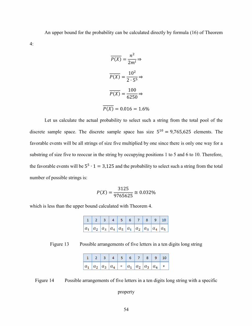
54

An upper bound for the probability can be calculated directly by formula (16) of Theorem

4:

𝑃(𝑋) =𝑛2

2𝑚𝑙⇒

𝑃(𝑋) =102

2 ∙ 55⇒

𝑃(𝑋) =100

6250⇒

𝑃(𝑋) = 0.016 = 1.6%

Let us calculate the actual probability to select such a string from the total pool of the

discrete sample space. The discrete sample space has size 510 = 9,765,625 elements. The

favorable events will be all strings of size five multiplied by one since there is only one way for a

substring of size five to reoccur in the string by occupying positions 1 to 5 and 6 to 10. Therefore,

the favorable events will be 55 ∙ 1 = 3,125 and the probability to select such a string from the total

number of possible strings is:

𝑃(𝑋) =3125

9765625≅ 0.032%

which is less than the upper bound calculated with Theorem 4.

Figure 13 Possible arrangements of five letters in a ten digits long string

Figure 14 Possible arrangements of five letters in a ten digits long string with a specific

property

55

However, let us assume that in the specific example the discrete sample space has been

constructed only by strings that have the following rule “each letter that occurs in positions 1 to 4

repeats with period 5 in the string.” Now, the string is definitely not random; and, therefore, not

normal and will have the format shown in “Figure 14”, where the * denotes any letter. Since each

letter in positions 1 to 4 is the same with each corresponding letter in positions 6 to 9 by definition

due to the rule, then we have to calculate the probability that the letters in positions 5 and 10 are the

same and, therefore, have a substring of length 5 that repeats in the string. The new discrete sample

space is of size 52 = 25 and the favorable events are 5. The probability to select a substring as

described in the example is:

𝑃′(𝑋) =5

25= 20%

The fact that the new string is not random because of the rule has increased the probability

to 20%, a value much higher than the upper bound 1.6% that Theorem 4 has estimated. ∎

Theorem 4 requests not only the initial string 𝑆 to be random but also to be “considerably”

long while substring 𝑠 to be “reasonably” long. If all conditions are met then the probability of a

substring 𝑠 of the initial string 𝑆 to occur at least twice in 𝑆 is “extremely” small. It is important to

mention that Theorem 4 asks for the substring 𝑠 just to be “reasonably” long and not “relatively”

long (i.e., compared to the initial string S), in order to have an extremely small probability. In the

above two examples, we were trying to explain how the mechanism of the upper bound for the

probability works and we haven’t used all prerequisites of the Theorem but only the randomness.

This is why in all the examples the probability calculated cannot be considered “extremely” small.

Let us now see what happens when all the prerequisites of the Theorem are met with the following

example:

56

Example 7. Suppose we have a fair coin and we flip it one million times. We record the flips

with 0’s for the tails and 1’s for the heads. Let’s try to answer the question “is the probability to get

50 zeros in a row at least twice in the million flips extremely small?” The string in our experiment

has length one million or approximately 220 = 1,048,576 (a power expressed in the base 2 of the

number which satisfies the Law of Large Numbers Theorem), the substring of 0’s has length 50

(satisfies the Normal Numbers) and the alphabet of the string has size 2 (the size of the set {0,1}).

The string is considerably long while the substring is reasonably long. We will use formula (16)

from Theorem 4 to calculate an upper bound for the probability of the event “50 zeros in a row to

occur at least twice in the one million long string:”

𝑃(𝑋)̅̅ ̅̅ ̅̅ ̅ =(220)2

2 ∙ 250=240

251=1

211≅ 0.05%

and the probability is small (1 out of 2048), yet, not extremely small. If instead of 50 zeros say we

ask for 100 zeros then an upper bound of the probability will be:

𝑃(𝑋)̅̅ ̅̅ ̅̅ ̅ =(220)2

2 ∙ 2100=240

2101=1

261

or 1 out of 2,305,843,009,213,693,952 (almost 2.3 million trillion). Now, the probability is

extremely small. The new substring of length 100 is reasonably long (yet, very close to 50) but its

length is insignificant compared to the initial string of length one million. Nevertheless, the

probability to occur is extremely small. Even if we flip the coin, say one trillion times (or

approximately 240) then the probability will be:

𝑃(𝑋)̅̅ ̅̅ ̅̅ ̅ =(240)2

2 ∙ 2100=280

2101=1

221

or 1 out of 2,097,152. Even now the probability is very small and we can convert it again to

extremely small value if we change the size of the reasonably long substring to 140 (once more

very close to 100), in order to have again 1 out of 2,305,843,009,213,693,952. ∎

57

So far, we have calculated an upper bound for the probability of a substring of specific

length to occur twice in a string. However, in our case we care to find an upper bound for the LERP

value so that the probability of a longer substring to occur twice to be insignificant. We need this

in order to ensure that there is no point to search for substrings with length greater than the LERP

value. For this purpose, we have constructed and proved the following Lemma.

Lemma 4. Let 𝑆 be a random string of size 𝑛, constructed from a finite alphabet 𝛴 of size 𝑚 ≥

2, and an upper bound of the probability 𝑃(𝑋) is 𝑃(𝑋), where 𝑋 the event “LERP is the longest

pattern that occurs at least twice in 𝑆.” An upper bound for the length 𝑙 of the Longest Expected

Repeated Pattern (LERP) we can have with probability 𝑃(𝑋) is:

𝑙 =

𝑙𝑜𝑔((𝑛 − 2𝑙 + 1)(𝑛 − 2𝑙 + 2))

2𝑃(𝑋)

𝑙𝑜𝑔𝑚<

⌈⌈⌈⌈ 𝑙𝑜𝑔

𝑛2

2𝑃(𝑋)

𝑙𝑜𝑔𝑚

⌉⌉⌉⌉

(21)

or

𝑙 ̅ =

⌈⌈⌈⌈ 𝑙𝑜𝑔

𝑛2

2𝑃(𝑋)

𝑙𝑜𝑔𝑚

⌉⌉⌉⌉

= ⌈𝑙𝑜𝑔𝑚𝑛2

2𝑃(𝑋)⌉ (22)

where 𝑙 ≪ 𝑛 and 𝑃(𝑋) > 0.

Proof:

From Theorem 4 we have that an upper bound for the probability of a substring 𝑠 of length

𝑙 to occur at least twice in a string of size 𝑛 is:

𝑃(𝑋) =(𝑛 − 2𝑙 + 1)(𝑛 − 2𝑙 + 2)

2𝑚𝑙⇔

𝑃(𝑋)2𝑚𝑙 = (𝑛 − 2𝑙 + 1)(𝑛 − 2𝑙 + 2) ⇔

𝑙𝑜𝑔 (𝑃(𝑋)2𝑚𝑙) = 𝑙𝑜𝑔((𝑛 − 2𝑙 + 1)(𝑛 − 2𝑙 + 2)) ⇔

58

𝑙𝑜𝑔 ( 2𝑃(𝑋)) + 𝑙𝑜𝑔𝑚𝑙 = 𝑙𝑜𝑔((𝑛 − 2𝑙 + 1)(𝑛 − 2𝑙 + 2)) ⇔

𝑙𝑜𝑔𝑚𝑙 = 𝑙𝑜𝑔((𝑛 − 2𝑙 + 1)(𝑛 − 2𝑙 + 2)) − 𝑙𝑜𝑔( 2𝑃(𝑋)) ⇔

𝑙 𝑙𝑜𝑔𝑚 = 𝑙𝑜𝑔((𝑛 − 2𝑙 + 1)(𝑛 − 2𝑙 + 2)) − 𝑙𝑜𝑔(2𝑃(𝑋)) ⇔

𝑙 =𝑙𝑜𝑔((𝑛 − 2𝑙 + 1)(𝑛 − 2𝑙 + 2)) − 𝑙𝑜𝑔(2𝑃(𝑋))

𝑙𝑜𝑔𝑚⇔

𝑙 =

𝑙𝑜𝑔((𝑛 − 2𝑙 + 1)(𝑛 − 2𝑙 + 2))

2𝑃(𝑋)

𝑙𝑜𝑔𝑚

𝑙≪𝑛⇒

𝑙 <

𝑙𝑜𝑔𝑛2

2𝑃(𝑋)

𝑙𝑜𝑔𝑚⇒

𝑙 ≅

𝑙𝑜𝑔𝑛2

2𝑃(𝑋)

𝑙𝑜𝑔𝑚

and since we need as an outcome an integer that represents an upper bound for the length of strings,

we can take the ceiling:

𝑙 <

⌈⌈⌈⌈ 𝑙𝑜𝑔

𝑛2

2𝑃(𝑋)

𝑙𝑜𝑔𝑚

⌉⌉⌉⌉

and we can select as the higher upper bound

𝑙 ̅ =

⌈⌈⌈⌈ 𝑙𝑜𝑔

𝑛2

2𝑃(𝑋)

𝑙𝑜𝑔𝑚

⌉⌉⌉⌉

and, hence, the Lemma has been proven. ⧠

Example 8. Let us take an example to calculate the value of LERP in a string 𝑆 with size |𝑆| =

𝑛 = 109 = 1,000,000,000 constructed from an alphabet of size |𝛴| = 𝑚 = 4. We want to

59

calculate the value of the LERP with an upper bound probability 𝑃(𝑋) = 10−2 = 0.01 = 1%.

From Lemma 4 we have:

𝑙 <

𝑙𝑜𝑔𝑛2

2𝑃(𝑋)

𝑙𝑜𝑔𝑚=𝑙𝑜𝑔

(109)2

2 ∙ 10−2

𝑙𝑜𝑔 4=𝑙𝑜𝑔

1018+2

2𝑙𝑜𝑔 4

=𝑙𝑜𝑔 1020 − 𝑙𝑜𝑔 2

𝑙𝑜𝑔 4⇒

𝑙 <20 − 0.301

𝑙𝑜𝑔 4=19.699

0.602= 32.723 ≅ 33

Therefore, with probability 1 − 0.01 = 0.99 or 99% we can store up to 33 characters long

substrings in the reduced suffix array in order to find all substrings of the string that occur at least

twice. Another way to express the probability is: the probability to find substrings longer than 𝑙 =

33 is only 1%. ∎

Example 9. As a last example, a thought experiment will be presented. Suppose that since the

beginning of time in the universe we have on each star a device that records every millisecond an

observation and now we have a single, long sequence of observations from all stars. Let us also

assume that the observations that have been recorded can take integer values from 0 to 9. In order

to estimate the length of this sequence we have to do first some calculations. Assuming that the age

of the universe is approximately 14.6 billion Earth years then we have:

𝑈𝑎𝑔𝑒 = 14.6 ∙ 109 ∙ 365 ∙ 24 ∙ 60 ∙ 60 ∙ 1,000 𝑚𝑠𝑒𝑐

Therefore, the age of the universe in milliseconds is approximately:

𝑈𝑎𝑔𝑒 ≅ 4.6 ∙ 1020 𝑚𝑠𝑒𝑐

Assuming that on average there exist (or existed) 100 billion galaxies and each one has (or

had) on average 100 billion stars, the total number of stars in the universe may be computed as:

𝑁𝑠𝑡𝑎𝑟𝑠 ≅ 1011 ∙ 1011 = 1022

The total number of observations and, therefore, the length of our sequence will be:

60

|𝑆| = 4.6 ∙ 1042

The above number is beyond any human imagination and it is impossible to construct such

a sequence with the current technology. However, assuming that it does exist and it is random, what

is the longest repeated pattern we expect to find in this sequence with a probability 1 out of a trillion

(0.0000000001%)? According to Lemma 4 we have:

𝑙 ̅ =

⌈⌈⌈⌈ 𝑙𝑜𝑔

𝑛2

2𝑃(𝑋)

𝑙𝑜𝑔𝑚

⌉⌉⌉⌉

= ⌈𝑙𝑜𝑔

(4.6×1042)2

2 ∙ 10−12

𝑙𝑜𝑔 10⌉ = ⌈𝑙𝑜𝑔

(4.6×1042)2

2 ∙ 10−12⌉ ≅ 𝑙𝑜𝑔 1097 = 97

Therefore, we expect that the longest repeated pattern will have length no longer than 97

with probability 1 1012⁄ . ∎

Our final step towards the completion of the theoretical foundations of LERP is to connect

Randomness with Normality. For this purpose, the following Preposition and Lemma have been

constructed and proven.

Preposition 1. Let 𝑆 be a string of size 𝑛, constructed from a finite alphabet 𝛴 of size 𝑚 ≥ 2. If the

string is Normal then Theorem 4 can be applied.

Proof:

The proof is a direct application of Calude’s [Calude 94] Theorem since every random string

is normal. Furthermore, by the definition of Normality each digit and each reasonably long

arrangement of digits should appear with the required frequency inside string 𝑆. Therefore, even if

a normal string is not random, Theorem 4 can be applied since Normality is a sufficient condition

by Theorem 4 and required by Calude’s Theorem [Calude 94]. ⧠

Lemma 5. Let 𝑆 be a string of size 𝑛, constructed from a finite alphabet 𝛴 of size 𝑚 ≥ 2. If the

string is Normal then Lemma 4 for the calculation of the LERP can be applied.

61

Proof:

The proof follows from a direct application of Calude’s [Calude 94] Theorem and

Preposition 1. ⧠

By constructing and proving Theorem 4 and Lemma 4 and the thought experiment of

Example 9, we have shown that we can construct a Reduced Suffix Array (i.e., with the actual

suffixes) of dimensions 𝑙×𝑛 for an enormous sequence, while the width 𝑙 of the suffix array can be

limited to just 100, assuming that the sequence is true random. Practically, the size of the Reduced

Suffix Array has asymptotic growth 𝑂(𝑐𝑛), where c is a constant extremely small compared to any

size of a given random sequence and definitely much less than 100 for any reasonably long random

string. Therefore, we can directly construct a Reduced Suffix Array in an external database

management system, in linear space required capacity, without any loss of information. Doing this,

provides us with an extreme advantage compared to any other use or storage of suffix arrays or

suffix trees since when our reduced suffix array is constructed it can be used at any time in the

future for further analysis and experiments without the need of reconstructing it again. Furthermore,

any experiment or analysis can be stopped at any given time, and thus releases our resources for

another purpose; the analysis may be resumed when the resources will be available again.

Concluding the theoretical aspect of the methodology there are some very important points that

need to be mentioned:

1) For strings of small length 𝑛, it is also expected to have small 𝑙. In this case, Theorem

4 returns values that are usually greater than 1 because the denominator of

expression (16) is much smaller than the nominator. Although, mathematically, a

probability cannot get such values, since 0 ≤ 𝑃(𝑋) ≤ 1, the theorem just proposes

an upper bound for the defined probability, and therefore, that is acceptable.

62

Otherwise, long strings are expected to contain longer repeated substrings, therefore,

the denominator of expression (16) is also expected to be greater than the nominator.

For example, if 𝑛 = 109 and 𝑙 = 20 then for an alphabet of 𝑚 = 4, the denominator

will be greater than 2 ∙ 1012 and, therefore, the upper bound for the probability of

the existence of a repeated substring with 𝑙 > 20 will be approximately 0.0005%.

2) LERP is just an upper bound for the occurrences’ length. It is not the supremum

(i.e., least upper bound) of occurrences’ length. However, this satisfies our work on

suffix arrays since with the use of LERP it is possible to reduce suffix array’s

required space capacity from millions of Terabytes to just Gigabytes, depending on

the nature of the original string (random or non-random) or in general we can reduce

the quadratic required space capacity of an array to linear.

3) In order the outcome of Theorem 4 to be valid and to be able to calculate with

relative accuracy 𝑙, the initial string has to be random and, therefore, normal.

Randomness and Normality may exist in number theory or chaotic models, however,

it may not exist in many cases with real-life variables, e.g., DNA. Yet, although

larger than the theoretical LERP, the actual LERP of non-random strings is

extremely small comparing to the string’s length. Even in cases with restrictions in

strings, the discrete sample space 𝛺(𝑆) is so huge that eventually the probability of

the event and 𝑙 will be very small compared to the size of the string. This fact allows

the implementation of the theory and the construction of very small reduced suffix

arrays, making the analysis of vast strings feasible.

4) Due to the fact that formulas (21) and (22) have logarithmic expression of the

parameters, no matter how fast 𝑛 grows or 𝑃(𝑋) shrinks, 𝑙 will grow with very small

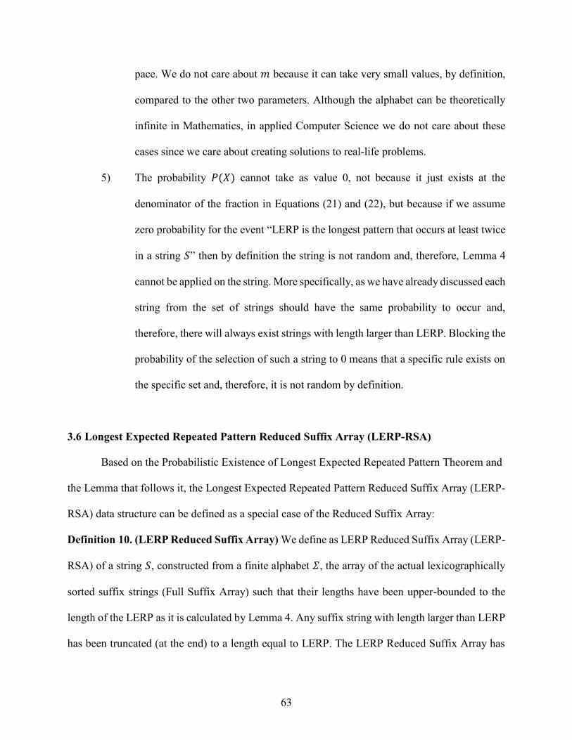
63

pace. We do not care about 𝑚 because it can take very small values, by definition,

compared to the other two parameters. Although the alphabet can be theoretically

infinite in Mathematics, in applied Computer Science we do not care about these

cases since we care about creating solutions to real-life problems.

5) The probability 𝑃(𝑋) cannot take as value 0, not because it just exists at the

denominator of the fraction in Equations (21) and (22), but because if we assume

zero probability for the event “LERP is the longest pattern that occurs at least twice

in a string 𝑆” then by definition the string is not random and, therefore, Lemma 4

cannot be applied on the string. More specifically, as we have already discussed each

string from the set of strings should have the same probability to occur and,

therefore, there will always exist strings with length larger than LERP. Blocking the

probability of the selection of such a string to 0 means that a specific rule exists on

the specific set and, therefore, it is not random by definition.

3.6 Longest Expected Repeated Pattern Reduced Suffix Array (LERP-RSA)

Based on the Probabilistic Existence of Longest Expected Repeated Pattern Theorem and

the Lemma that follows it, the Longest Expected Repeated Pattern Reduced Suffix Array (LERP-

RSA) data structure can be defined as a special case of the Reduced Suffix Array:

Definition 10. (LERP Reduced Suffix Array) We define as LERP Reduced Suffix Array (LERP-

RSA) of a string 𝑆, constructed from a finite alphabet 𝛴, the array of the actual lexicographically

sorted suffix strings (Full Suffix Array) such that their lengths have been upper-bounded to the

length of the LERP as it is calculated by Lemma 4. Any suffix string with length larger than LERP

has been truncated (at the end) to a length equal to LERP. The LERP Reduced Suffix Array has

64

one column for the index of the position where each suffix string occurs in the string and another

column for the reduced suffix strings.

The above definition presents the importance of the theoretical calculation of LERP

because:

1) It does not require any prior construction of any data structure, which may be

unfeasible or extremely time consuming, and

2) It is the optimal value we can take in order to construct the Reduced Suffix Array

of Definition 10.

More specifically, Lemma 4 guarantees with high probability that the LERP value should

be bound from the outcome of Formula (22). Therefore, if we choose as LERP a value larger than

the outcome of Formula (22) we need more space in order to construct the LERP-RSA data

structure, while if we choose as LERP a value smaller than the outcome of Formula (22) we lose

information since repeated strings with length up to LERP will exist with high probability.

3.7 LERP-RSA Advanced Characteristics

3.7.1 Classification

Definition 11. (LERP-RSA Classification Level) We define as Classification Level 𝐶𝐿 of the

LERP-RSA, the power L to which the alphabet size |𝛴| should be raised in order to calculate the

number of the desired classes we want to partition the LERP Reduced Suffix Array:

𝐶𝐿 = |𝛴|𝐿

L can take any positive integer value, 𝐿 ∈ 𝑁, starting from 0:

𝐶0 = |𝛴|0 = 1

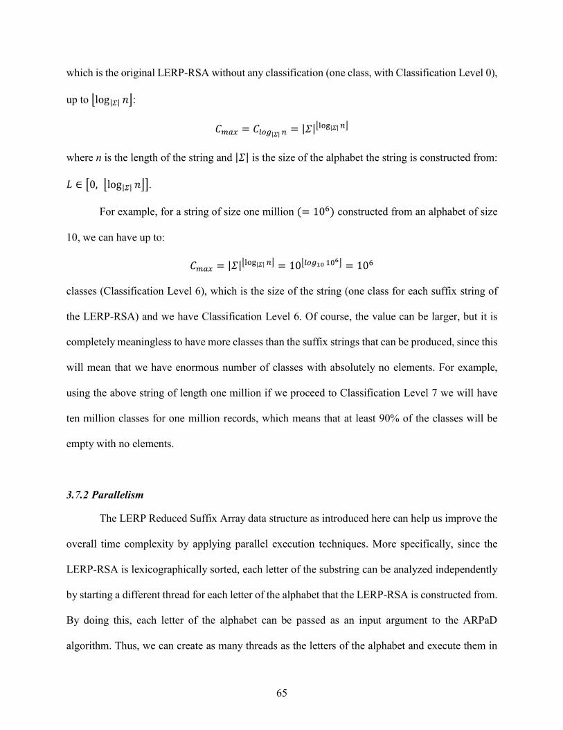
65

which is the original LERP-RSA without any classification (one class, with Classification Level 0),

up to ⌊log|𝛴| 𝑛⌋:

𝐶𝑚𝑎𝑥 = 𝐶𝑙𝑜𝑔|𝛴| 𝑛 = |𝛴|⌊log|𝛴|𝑛⌋

where n is the length of the string and |𝛴| is the size of the alphabet the string is constructed from:

𝐿 ∈ [0, ⌊log|𝛴| 𝑛⌋].

For example, for a string of size one million (= 106) constructed from an alphabet of size

10, we can have up to:

𝐶𝑚𝑎𝑥 = |𝛴|⌊log|𝛴| 𝑛⌋ = 10⌊𝑙𝑜𝑔10 10

6⌋ = 106

classes (Classification Level 6), which is the size of the string (one class for each suffix string of

the LERP-RSA) and we have Classification Level 6. Of course, the value can be larger, but it is

completely meaningless to have more classes than the suffix strings that can be produced, since this

will mean that we have enormous number of classes with absolutely no elements. For example,

using the above string of length one million if we proceed to Classification Level 7 we will have

ten million classes for one million records, which means that at least 90% of the classes will be

empty with no elements.

3.7.2 Parallelism

The LERP Reduced Suffix Array data structure as introduced here can help us improve the

overall time complexity by applying parallel execution techniques. More specifically, since the

LERP-RSA is lexicographically sorted, each letter of the substring can be analyzed independently

by starting a different thread for each letter of the alphabet that the LERP-RSA is constructed from.

By doing this, each letter of the alphabet can be passed as an input argument to the ARPaD

algorithm. Thus, we can create as many threads as the letters of the alphabet and execute them in

66

parallel, by using the appropriate hardware configuration, i.e., a computer with multiple single-core

processors or a multi-core processor. This technique can significantly reduce the total time needed

for the execution of the ARPaD algorithm, roughly down to the time needed for the most time-

costly thread. Of course, when the analysis is executed on a single CPU, we have to take into

consideration the overhead from the operating system to control and execute parallelism. However,

as described in the next paragraph (3.7.3), we can execute each thread in different CPUs in parallel

and, therefore, avoid this overhead. If we assume that all threads need the same amount of time to

complete the execution, the total time will be exactly the fraction of the single thread execution time

over the number of letters in the alphabet. For example, if we have a sequence constructed from an

alphabet of four letters then the total time needed for execution will be approximately 1/4 of the

total time required for sequential execution.

3.7.3 Semi-Parallel Classification/Execution

By further taking into account the LERP-RSA data structure as it has been introduced here,

data classification can be used in combination with parallelism in order to improve speed and the

required space capacity. By applying a divide and conquer strategy, instead of creating one large

database to store the whole LERP-RSA, we can partition the LERP-RSA to different significantly

smaller parts optimized for immediate input to the threads, and store each (sub) LERP-RSA to a

unique table in the database. So, instead of each thread previously created to send queries to a huge

suffix array table in the database simultaneously, we can alter the process and lead each thread to

retrieve the required data from a unique table created for each (sub) LERP-RSA. This technique

has many advantages since the tables that will be created are much smaller than the original LERP-

RSA table and, therefore, they consume much less space and the total time needed for sorting will

67

be considerably shorter. Furthermore, we can avoid bottlenecks in the communication with the

database management system since each query, which will be sent to the database, will target a

different table instead of having many queries accessing the same table simultaneously.

Again, it is important to mention that this technique needs the support of the appropriate

hardware and software infrastructure since the database management system must support multi-

processing and the hardware should allow to create all classes and run all threads in parallel. Yet,

this is unfeasible when the string is extremely large and the produced LERP-RSA is expected to

exceed the limits of the hard disk or when the Classification Level is larger than one and we need

hundreds or thousands of threads to execute in parallel. In this case, as mentioned in the previous

paragraph, we can apply a combination of Classification-Parallelism in a Semi-

Parallel/Classification execution. First, we have to decide what Classification Level we will use.

Then we group our classes based on the Classification Level we have used minus one and execute

the analysis of this group of classes in parallel. For example, let us assume that we want to analyze

a string of length 10 billion constructed from an alphabet of size 10 (e.g. 0 to 9) by using a

Classification Level 2, which will build 100 classes. The LERP for such a string is 22 and, therefore,

it is not possible to construct the LERP-RSA (assuming small hard disk) and run 100 threads in

parallel for the Classification Level 2. However, we can construct the ten classes of the first

character of the alphabet first, i.e., 00 to 09, and analyze in parallel using ten threads. This approach

seems like a Classification Level 1, yet, it is a Semi-Parallel/Classification execution of a

Classification Level 2. After completing the first ten classes we can delete the LERP-RSA data

structure, free the space occupied and continue with the next alphabet character 1 and classes 10 up

to 19. We will repeat this process as many times as the characters of the alphabet. Although this

method is slower, it allows us to analyze any kind of string regardless of the length it has and the

68

hardware we use. We can easily overcome the problem of string size and hardware limitations, by

using any kind of different grouping based on different Classification Levels, e.g., Classification

Level 3 with 1,000 classes and analyze 20 classes with 20 threads in each cycle. We just need to

optimize this process for the hardware we have available each time.

3.7.4 Network/Cloud Distribution and Full Parallel Execution

The fact that LERP Reduced Suffix Arrays can be constructed and stored to external media,

instead of memory like suffix trees or suffix arrays, allows the use of distributed network and cloud

computing techniques. Instead of using one super computer with multi-processors, we can split the

LERP-RSA to a vast number of sub-classes/tables and store each one in a different computer over

a local network of computers, the cloud or even any kind of electronic computing device. Since

each sub-class can be stored in an independent table in a database, they can also be stored in

different databases installed in different computers. Each computer can then execute the ARPaD

algorithm to analyze the specific sub-class and return the results to a central server for further

analysis. One more advantage of such distribution is that we can avoid the use of DBMSs since the

classes can be extremely small in size and can be distributed using simple text files that can be

easily loaded and analyzed by ARPaD directly in memory. This means that any electronic

computing device such as smartphones can be used for such an analysis without the need of an

advanced DBMS to exist on the device.

We can present the following example of the above described technique that will allow us

to argue the novelty and importance of the methodology described in the current thesis. Assume

that we want to analyze a string of size 100 Terabytes constructed from an alphabet of size 10.

Theoretically, using a classical suffix array or suffix tree data structure we need significantly more

69

than 2,000 Terabytes of RAM and significantly more amount of disk space in order to conduct the

analysis on a single computer, something which can easily be characterized as impossible for

standard desktop computers. With the currently presented methodology we can partition the LERP-

RSA to a Classification Level 7 and create ten million classes, 𝐶7 = 107 = 10,000,000. Each class

will have approximately (if all classes are equidistributed) 10,000,000 suffix strings (records) of

size 30 digits according to Lemma 4. This means that the total size of each class is approximately

300 MB. Each class can now be easily distributed to any kind of computing device and analyzed

using the ARPaD algorithm and the results submitted back to a central server. Such an analysis can

easily be done by any smartphone since nowadays smartphones have very good processors and a

few GB of storage, enough for the specific amount of data.

The possible use of common electronic devices, such as smartphones, has been mentioned

in order to emphasize the ability of the LERP-RSA data structure to scale up and be used for the

analysis of big data on regular computer systems. For example, the analysis of a string of size 100

Gigabytes can be impossible or extremely slow in an academic environment where hardware

resources are usually limited to few average personal computers. Another option could be a

supercomputer or cluster-computing framework, which are not easily accessible resources and

definitely are very expensive. However, let’s assume that a university has 40,000 students, half of

whom (i.e., 20,000) have smartphones and half of these students (i.e., 10,000) are willing to share

their smartphones for the execution of the experiment. This means we can work with Classification

Level 4 (10,000 classes) of size approximately 10 million records of length 22 and overall memory

usage of approximately 300MB. The creation of the table, sorting and execution of the ARPaD

algorithm is a process that (for such datasets) needs on average 10 to 15 minutes on a standard PC

if we execute the process using a DBMS on a disk and not directly in memory. Even if we assume

70

that we need double the time to execute the experiment on a smartphone memory compared to a

PC, this is feasible and are unlikely problems such as battery exhaustion before completing the

experiment, since we have to process only 300MB.

3.7.5 Compression

Another important advantage of the specific data structure is that we can further compress

each class and, therefore, achieve self compression of the data structure. Since each class holds

strings starting with the specific class digits arrangement, these digits can be omitted to reduce the

size of the class by the related percentage. For example, by applying a Classification Level 2 in a

LERP-RSA over the decimal alphabet of size 10 it means that we will have 100 classes starting

from 00 up to 99. Each class holds all the suffix strings that start with the class designated digits,

e.g., class 00 has all suffix strings starting with 00, class 01 has all the suffix strings starting with

01, etc. Therefore, for each of these 100 classes we can omit the first two digits since they are

redundant and have no information to lose by this omission. It is important though to remember

that after the completion of the analysis the strings which were found are missing the first two

digits and, therefore, we have to insert them in front of each string discovered. This process can

be avoided by simply saving the results that have been found to similarly named tables, like the

classes, something that will imply the compression used. Using the previous example of the 100

trillion digits string and the ten million classes, the first 7 digits of each class are exactly the same.

This means that 7 out of 30 digits can be omitted and the final space required by the class is not

300 MB but approximately 230 MB (= 10,000,000 ∙ 23) which is almost 24% less than the

required space.

71

3.7.6 Indeterminacy

An additional very important and unique property that LERP-RSA has is Indeterminacy

which gives LERP-RSA significant flexibility compared to the original Suffix Array data structure,

as introduced by Manber and Myers [Manber and Myers 90], but also other data structures related

to pattern detection.

Definition 12. (FSA, RSA and LERP-RSA Indeterminacy State) It is defined that a Full Suffix

Array, RSA or LERP-RSA is in Indeterminacy State when the positions of the suffix strings have

been removed and the Full Suffix Array, RSA or LERP-RSA have only one column with the actual

suffix strings “Figure 15.b” and “Figure 15.d”.

Although information regarding the position of each suffix string in the Full Suffix Array

and LERP-RSA has been lost when the Full Suffix Array or LERP-RSA are in Indeterminacy

State, however, the actual suffix strings still exist and can be used for pattern detection purposes.

There are many cases when we do not care about the position of the patterns in a sequence, rather

we care only about the patterns themselves, as it will be presented in Chapter 5 with the

applications in Transaction Analysis, Network Security, Clickstream Analysis and Number

Theory. Something like this cannot be performed with the original Suffix Array data structure, as

introduced by Manber and Myers [Manber and Myers 90], simply because the Suffix Array is the

array of the indexes of the lexicographically sorted suffix strings. By omitting these indexes the

data structure is destroyed.

When the LERP-RSA is used for Big Data Mining in large sequences of lengths greater

than 232 then the indexes of the suffix string positions have to be constructed using a 64bit integer

representation, which means that they occupy 8 bytes. This property is very important and gives

extreme flexibility in the LERP-RSA regarding the space it is required to be stored in because in

72

combination with the Compression of paragraph 3.7.5 the total compression of the LERP-RSA

can reach levels close to or above 50% if it is allowed to omit the suffix strings positions.

Figure 15 Full Suffix Array and LERP-RSA in Indeterminacy State

73

Chapter 4 Advanced Algorithms for Pattern Detection in Big Data

4.1 Introduction

This chapter introduces two different categories of algorithms of the current thesis. The

first category includes the algorithms required in order to create the Full Suffix Array and the

Reduced Suffix Array with or without the use of the LERP. The second category covers the most

important algorithms which, based on the previously created data structure, allow the detection of

single, multiple and all repeated patterns, with or without the use of wildcards. These algorithms

have exceptional behavior and, in combination with the LERP-RSA data structure, allow the

analysis of big data in a short time and with limited resources. Finally, one more algorithm will be

presented, the Moving LERP, which allows using the algorithms in the two categories in cycling

phases to detect all repeated patterns despite any kind of hardware limitation (e.g., memory or

disk) which could make such an analysis infeasible.

Part of the material covered in this chapter has been published in fully refereed journals or

presented in conferences and published in the corresponding proceedings [Xylogiannopoulos et al.

12a, 12b, 12c, 14a, 14b, 16b].

4.2 Construction of Full, Reduced and LERP-Reduced Suffix Array

4.2.1 Full Suffix Array Construction (FSAC)

In order to create the full suffix array, we use a simple algorithm, which in each loop

removes the first digit from the sequence (initially) or the suffix string (for all other strings) and

stores the remaining in the database with the appropriate index of occurrence (see Algorithm 1).

The Algorithm terminates and it is correct since in each loop removes the first digit of the reminder

74

of the string and when it reaches the last digit the for-loop terminates. The Algorithm has

complexity 𝑂(𝑛) since it is a simple for-loop up the length 𝑛 of the string.

4.2.2 Reduced Suffix Array LERP-RSA Construction (ORSAC)

For the advanced construction of the Reduced Suffix Array and the RSA using LERP,

Algorithm 2 can be used. ORSAC is a variation of FSAC since it saves in the database each time

the first part of the suffix string with length either the reduced length l or the LERP length, as

defined in the input arguments. If the length of the suffix string becomes smaller than l or LERP

(i.e., for the last l or LERP positions of the string) then it saves the suffix string as it is.

Algorithm 1. Full Suffix Array Construction (FSAC)

Input: string S of sequence

Output: an array of all suffix strings or nothing in case of direct insertion into database

1 FSAC(string S)

2.1 for i := 0; i< S.length; i++

2.2 subString := S.Substring(i, S.length – i)

2.3 insert substring into database

2.4 end for

3 end FSAC

Algorithm 2. Optimized Reduced Suffix Array Construction using LERP (ORSAC)

Input: string S of sequence

Output: an array of all suffix strings or nothing in case of direct insertion into the database

1 ORSAC (string S, int LERP)

2.1 for i := 0; i<S.length; i++

2.2.1 if (LERP + i>S.length)

2.2.2 LERP :=X.length-i

2.2.3 end if

2.3 subString :=S.Substring(i, LERP)

2.4 insert substring into database

2.5 end for

3 end ORSAC

75

4.3 All Repeated Patterns Detection (ARPaD) Algorithms Family

In the current paragraph the family of the All Repeated Patterns Detection (ARPaD)

Algorithms will be presented. To date, the recursive version of the ARPaD algorithm has been

presented in publications [Xylogiannopoulos et al. 12a, 12b, 14a, 14b]. However, one more

version, non-recursive this time, will be presented in this thesis, which also takes full advantage

of the previously introduced LERP-RSA data structure. Both versions of ARPaD algorithm have

several variations depending on how initial parameters have been set regarding the use of Full

Suffix Array or LERP-RSA and the use of Shorter Pattern Length (SPL), which allows the

detection of patterns with length above a predefined threshold. Although LERP value in LERP-

RSA has a very important role since it defines the creation of the data structure, for the ARPaD

algorithm LERP can also be used as an upper bound threshold to detect patterns with length below

a predefined threshold, smaller than LERP, something analogous to the use of SPL.

Moreover, the ARPaD algorithm allows the use of several other filters, except SPL and

LERP, leading to a vast number of variations of the original, basic, ARPaD algorithm. For

example, a filter could be the detection of patterns with even length or with odd length only.

Another version could be the use of a specific length filter or the use of a filter for patterns with

unique attributes when we have a problem and we need to detect extraordinary patterns. For

example, in text mining we may need to detect words that have specific length and which also start

with a specific letter or include a specific combination of letters. This is also important in

transactions and clickstreams analysis if we need to detect itemsets which include specific items

only.

However, in most cases these variations are problem specific only (such as transactions

analysis or network security as we will see in Chapter 5) since the use of filters increases the

76

complexity of the algorithm. Furthermore, if the initial parameters of the problem are changed this

means that the algorithm has to be executed again making the whole process time consuming. The

general version of the ARPaD algorithm is the simplest and best solution in most cases because

one of the unique characteristics is that it detects every repeated pattern. Then, every problem

specific analysis can be executed directly on the results as a meta-analysis without the need to

reconstruct the data structure and execute the algorithm again.

The use of such filters allows us to create endless variations of the ARPaD, which are

impossible to be listed in a thesis since it is out of scope of algorithmic design and analysis as they

are minor variations of the original, fundamental, ARPaD algorithm.

4.3.1 Recursive ARPaD

4.3.1.1 ARPaD Algorithm Using Full Suffix Array

The first variation of the All Repeated Patterns Detection (ARPaD) Algorithm follows

below. It is the one that allows the simple detection of all repeated patterns without any kind of

limitation or initial parameters. In order to calculate all repeated patterns that exist in a sequence

the following process has to be executed:

1) For all the letters of the alphabet count suffix strings that start with the specific

letter.

2) If no suffix strings are found or only one is found, proceed to the next letter

(repetition cannot be defined with just one occurrence.)

3) In the event that the number of substrings found is the same as the total number of

suffix strings, proceed to step 4; the specific letter can be considered as a non-

significant occurrence because a longer hyper-string will occur.

77

4) If more than one string and less than the total number of suffix strings are found,

then, for the letter used and counted already and for all letters of the alphabet, add

a letter at the end and construct a new hyper-string. Then do the following checks:

a) If none or one suffix string is found that starts with the new hyper-string,

consider the previous substring as an occurrence and proceed with the next

letter of the alphabet.

b) If the same number of substrings is found as previously then proceed to step

4. However, the specific substring can be considered as a non-significant

occurrence because a longer hyper-string will occur.

c) If more than one and less than the number of occurrences of the previous

substring are found, consider the previous substring as a new occurrence

and continue the process from step 4.

78

Example 10. In the case of the string kananaskis, the following process has been used: Starting

with the first letter of the alphabet, a, three substrings can be found that start with a “Figure 16.a”.

Since more than one and less than the total number of substrings of the suffix array have been found

starting with a, the process should continue to search deeper by adding each letter of the alphabet

to 𝑎 and constructing a new string each time. The first hyper-string is aa. Since there is no substring

starting with aa, the process should continue with the next letter and the creation of a new hyper-

string, namely ai. However, no strings start with ai either. The algorithm continues with the next

letter k. Again, no strings start with ak and the algorithm proceeds to the next letter n. Counting the

substrings that start with the new string an, the result is one less than the previous string (with only

one letter, a), see “Figure 16.b”. In this case, the first string that the process started with, i.e., a, is

Algorithm 3. All Repeated Patterns Detection Using Full Suffix Array (ARPaD-FSA)

Input: string X of pattern we want to check, a counter of string length

Output: a list of all occurrences

1 ARPaD_FSA(string X, int count)

2 isXcalculated := false

3.1 for each letter l in alphabet

3.2 newX := X + l

3.3 newCount := how many strings start with newX

3.4.1 if newCount = count

3.4.2 ARPaD_FSA(newX, newCount)

3.4.3 end if

3.5.1 if (newCount = 1) AND (isXcalculated = false) AND (X NOT null)

3.5.2 find positions of string X

3.5.3 isXcalculated := true

3.5.4 end if

3.6.1 if newCount > 1 AND newCount < count

3.6.2.1 if (isXcalculated = false) AND (X NOT null)

3.6.2.2 find positions of string X

3.6.2.3 isXcalculated := true

3.6.2.4 end if

3.6.3 ARPaD_FSA(newX, newCount)

3.6.4 end if

3.7 end for

4 end ARPaD_FSA

79

definitely a significant occurrence because the hyper-string 𝑎𝑛 has occurred less times in the

sequence. The algorithm continues to search for longer strings than an by repeating the process for

every letter of the alphabet and starting again with the a and it founds the string 𝑎𝑛𝑎 that occurs

exactly as many times as the string an. Since 𝑎𝑛𝑎 is longer than an, the process uses then the longer

string, i.e., ana. Continuing to search deeper by adding again each one of the alphabet letter to the

new string ana, the process starts with the letter a and continues until it covers all the letters of the

alphabet without finding a longer repeating string than ana, see “Figure 16.c”. Therefore, ana is a

significant occurrence. Then the process goes back to step 4 and checks for string as. Since there is

only one substring starting with as, the process will finish with all the substrings starting with a. So

far, the occurrences that are significant are a and ana. By continuing the process and moving back

to the first step and proceeding with the other letters of the alphabet, the process will detect the

occurrences k, na and s. So, the whole process has been concluded and produced the following

findings as presented in “Figure 16.d”.

Figure 16 The repeated patterns of string kananaskis using ARPaD-FSA

In the algorithm, there are two outside calls: (a) the “how many strings start with new X”,

which queries the database and returns the number of the strings that start with the specific

80

substring and (b) the “find positions of string X”, which gets the positions of the suffix strings in

the sequence. These positions are the numbers in front of each suffix string. In the specific example

with string kananaskis, the occurrences 𝑎, 𝑎𝑛𝑎, k, 𝑛𝑎 and 𝑠 have been found and the equivalent

occurrence vectors are: 𝑎(1, 3, 5), 𝑎𝑛𝑎(3, 6), 𝑘(0, 7), 𝑛𝑎(2, 4) and 𝑠(6, 9).⧠

4.3.1.2 ARPaD Algorithm Using Full Suffix Array and Shorter Pattern Length (ARPaD-

SPL)

The ARPaD-SPL algorithm allows the detection of patterns that are larger than a specific

length (shorter pattern length). This is very important because usually when analyzing large

sequences, like DNA, very short patterns of length 1, 2, 3, etc. while they are not important the

detection of them is very time consuming. The storage of all positions of these patterns requires

significant amount of space. The ARPaD-SPL algorithm can be described as follows:

1) For all letters of the alphabet count suffix strings that start with the specific letter.

2) If no suffix strings found or only one is found, proceed to the next letter (periodicity

cannot be defined with just one occurrence.)

3) In case the same number of substrings is found as the total number of the suffix

strings, proceed to step 4 and the specific letter is not considered as an occurrence

because a longer hyper-string will occur.

4) If more than one string and less than the total number of the suffix strings is found,

then for the letter used and counted already and for all letters of the alphabet add a

letter at the end and construct a new hyper-string. Then do the following checks:

a) If none or one suffix string is found that starts with the new hyper-string

and the length of the previous substring is equal to or larger than SPL,

81

consider the previous substring as an occurrence, find the previous

substrings’ positions and proceed with the next letter of the alphabet.

b) If the same number of substrings is found as previously then proceed to step

4. However, the specific substring can be considered as a non-significant

occurrence because a longer hyper-string will occur.


substring is found, consider the previous substring as a new occurrence. If

the previous substring has not been calculated again and the length of the

substring is equal to or longer than SPL then calculate substrings’ positions.

Continue the process from step 4.

Algorithm 4. All Repeated Patterns Detection Using Shorter Pattern Length (ARPaD-SPL)

Input: string of pattern X we want to check, a counter of string length, SPL length


1 ARPaD_SPL(string X, int count, int SPL)



3.2 newX := X + l


3.4.1 if (newCount = count)

3.4.2 ARPaD_SPL(newX, newCount, SPL)

3.4.3 end if

3.5.1 if (newCount=1) AND (isXcalculated = false AND (X NOT null) AND X.length>=SPL)



3.5.4 end if

3.6.1 if (newCount > 1) AND (newCount < count)

3.6.2.1 if (isXcalculated = false) AND (X NOT null) AND (X.length >= SPL)



3.6.2.4 end if

3.6.3 ARPaD_SPL(newX, newCount, SPL)

3.6.4 end if

3.7 end for

4 end ARPaD_SPL

82

4.3.1.3 ARPaD Algorithm Using LERP Reduced Suffix Array and SPL

The ARPaD algorithm which uses a suffix array constructed based on a LERP value can

detect patterns of length larger than SPL and with length 𝑙 at most LERP. Like in the previous

section, usually we care about patterns with length larger than a specific minimum (SPL) and shorter

than a specific maximum (LERP). Of course, ARPaD can be used with different initial parameters

𝑆𝑃𝐿 ≥ 1 and 𝑙 ≤ 𝐿𝐸𝑅𝑃. The execution of the algorithm can be in different cycles to produce the

desired results to the user. For instance, for an experiment in DNA sequence we might care about

patterns with length between 7 and 15 (first phase of execution) and also for pattern with length

between 20 and 30 (second phase of execution). This technique can be expanded as the user of the

algorithm needs, in order to retrieve the appropriate results. In other words, this can be customized

to satisfy the needs of every need in data mining and pattern detection. ARPaD algorithm can be

described as follows:

1) For all letters of the alphabet, count suffix strings that start with the specific letter.

2) If no suffix strings are found or only one is found, proceed to the next letter

(periodicity cannot be defined with just one occurrence.)

3) In case the same number of substrings is found as the total number of the suffix

strings, proceed to step 4 and the specific letter can be considered as a non-

significant occurrence because a longer hyper-string will occur.

4) If more than one string and less than the total number of the suffix strings is found,

then for the letters used and counted already and for all letters of the alphabet add

a letter at the end and construct a new hyper-string. Then do the following checks:

a) If none or one suffix string is found that starts with the new hyper-string

and the length of the previous substring is equal to or larger than SPL and

smaller than LERP, consider the previous substring as an occurrence, find

83

previous substrings’ positions and proceed with the next letter of the

alphabet.

b) If the same number of substrings is found as previously and the length of

the previous substring is smaller than LERP then proceed to step 4.

However, the specific can be considered as a non-significant occurrence

because a longer hyper-string will occur.


substring is found and the length of the previous substring is different than

LERP, consider the previous substring as a new occurrence. If the previous

substring has not been calculated again and the length of the substring is

equal to or longer than SPL then calculate substrings’ positions. Continue

the process from step 4.

Figure 17 The repeated patterns of string kananaskis using a ARPaD with 𝐿𝐸𝑅𝑃 = 3

84

4.3.1.4 ARPaD Algorithm Correction

First, we will show that the ARPaD algorithm terminates and then we will use reductio ad

absurdum to prove its correctness.

Termination: First of all, the algorithm is finite since the alphabet is finite. It works in a recursive

way, increasing each time the length of the pattern to detect by one for each one of the alphabet’s

letters. If the length of the pattern under examination reaches the value of LERP, the ARPaD

Algorithm 5. All Repeated Patterns Detection with Shorter Pattern Length and Longest

Expected Repeated Pattern

Input: string of pattern X we want to check, a counter of string length, SPL length, LERP

length


1 ARPAD (string X, int count, int SPL, int LERP)



3.2 newX := X + l


3.4.1 if (newCount = count) AND (X.length < LERP)

3.4.2 ARPAD (newX, newCount, SPL, LERP)

3.4.3 end if

3.5.1 if (count > 1) AND (X.length = LERP) AND (isXcalculated = false)



3.5.4 end if

3.6.1 if (newCount=1) AND (isXcalculated = false) AND (X NOT null) AND (X.length>=SPL)



3.6.4 end if

3.7.1 if (newCount > 1) AND (newCount < count) AND (X.length <> LERP)

3.7.2.1 if (isXcalculated = false) AND (X NOT null) AND (X.length >= SPL)



3.7.2.4 end if

3.7.3 ARPAD (newX, newCount, SPL, LERP)

3.7.4 end if

3.8 end for

4 end ARPAD

85

Algorithm will terminate at line 3.4.1 or 3.5.1. Alternatively, it will clear the value of LERP and

continue from the SPL value with the next alphabet letter (line 3.2) until it will consume all the

alphabet (see the for-loop at line 3.1). ■

Correctness: Let’s suppose that the algorithm fails to identify all repeated patterns that have a

specific prefix in the suffix strings array. In this case, we can identify three different occasions:

1) The length of the pattern is less than SPL. In this case, the ARPaD Algorithm in

lines 3.6.- and 3.7.2.- bypassed the detection of the pattern, which is correct since

we have specifically asked to detect patterns that have length larger than or equal to

SPL.

2) The length of the pattern is larger than LERP. In this case, the ARPaD Algorithm in

lines 3.4.- and 3.5.- stops the detection of the pattern, which is correct since we have

specifically asked to detect patterns that have length less than or equal to LERP.

3) The length of the pattern is equal to or larger than SPL and less than or equal to

LERP. Since the algorithm failed to detect the repeated pattern, therefore, there is at

least one repeated pattern that exists with length 𝑙, where 𝑆𝑃𝐿 ≤ 𝑙 ≤ 𝐿𝐸𝑅𝑃.

Therefore, there are at least two suffix strings with the same starting substring that

the algorithm failed to identify; they have the same length 𝑙,where 𝑆𝑃𝐿 ≤ 𝑙 ≤

𝐿𝐸𝑅𝑃. Therefore, in order to fail to detect these substrings the algorithm stopped at

position 𝑙 − 1. This means that the algorithm checked the patterns of length 𝑙 − 2

and found them to be equal and stopped at length 𝑙 − 1 because it checked them and

found that they were not equal. However, this is a contradiction because the

substrings of length 𝑙 − 1 are equal and the algorithm cannot stop there and since it

has already checked the patterns of length 𝑙 − 1 (since it stopped there) in lines 3.5.-

86

and 3.6. Therefore, the algorithm will continue from position 𝑙 and it will detect the

repeated patterns of length 𝑙. Therefore, a repeated pattern that the algorithm will

fail to detect cannot exist and, hence, the algorithm has been proven to be correct. ■

4.3.1.5 ARPaD Algorithm Analysis

In order to calculate the theoretical worst case complexity of the ARPaD algorithm we can

use as an example a very bad sequence in which small patterns repeat and construct longer which

are substrings of longer patterns etc., e.g., abcabcabcabcabc. This process can be repeated as many

times as the length of the sequence. In such a sequence alphabet letters are equidistributed and,

therefore each partition has length 𝑛

𝑚, where m is the size of the alphabet. In each partition the

longest patterns will have length k, where k can be in general any positive natural number but in the

above example of repeating a has exactly the value LERP. The ARPaD algorithm for each pattern

needs exactly log𝑚𝑛

𝑚𝑘= log𝑚 𝑛 − log𝑚𝑚

𝑘 = log𝑚 𝑛 − 𝑘 runs to detect the pattern and has to

repeat the process 𝑛

𝑚 times for each partition. Therefore, the total runs for ARPaD algorithm for all

alphabet letters will be 𝑚𝑛

𝑚(log𝑚 𝑛 − 𝑘) = 𝑛(log𝑚 𝑛 − 𝑘) = 𝑛 log𝑚 𝑛 − 𝑛𝑘 and the complexity

of the algorithm for the worst case will be 𝑂(𝑛 log𝑚 𝑛 − 𝑛𝑘) or in general 𝑂(𝑛 log𝑚 𝑛). By worst

case, we describe sequences that are deliberately created to have extremely bad structure, e.g.,

having a small repeated pattern that constructs longer repeated patterns as the sequence grows as

described above. For this kind of testing, artificial sequences had to be constructed in order to allow

the testing of the algorithm, since no other naturally created sequence could meet such kind of

criteria to be characterized as worst case. With the use of SPL, the overall worst case complexity of

the ARPaD Algorithm is again of type generally 𝑂(𝑛 log𝑚 𝑛) in worst case. However, the

experimental findings reported in several publications [Xylogiannopoulos et al. 12a, 12c, 14b] have

87

shown a time complexity for the average case scenario of type linear, i.e., 𝑂(𝑛), for every variation

of ARPaD algorithm, including ARPaD-LERP. [Xylogiannopoulos et al. 14b].

4.3.2 Non-Recursive ARPaD

The Non-Recursive version of ARPaD algorithm, using SPL and LERP, will be presented

here. As with the recursive version of ARPaD algorithm, we are usually interested in patterns with

length larger than or equal to a specific minimum (SPL) and shorter than or equal to a specific

maximum (LERP). Again, Non-Recursive ARPaD can be used with different initial parameters

𝑆𝑃𝐿 ≥ 1 and 𝑙 ≤ 𝐿𝐸𝑅𝑃. The Non-Recursive ARPaD algorithm can be described as follows:

1) For every element (suffix string) in LERP-RSA after the first one repeat.

a. For every substring of each element (suffix string) with length from SPL up

to LERP repeat.

i. If substring is equal to the same length substring of the previous

element then increase length counter and store position of previous

suffix string.

ii. If substring is not equal to the same length substring of the

previous element and length counter is greater than one then store

the previous element substring position and substring as repeated

pattern. Reset counter from this length.

88

4.3.2.1 N-R ARPaD Algorithm Correction

The Non-Recursive ARPaD Algorithm proof of correctness is much simpler than the

recursive the ARPaD since it is a two nested loops algorithm.

Termination: The Non-Recursive ARPaD algorithm terminates because, firstly, it runs over all 𝑛

elements of a LERP-RSA data structure in the outer loop or any class of a LERP-RSA in case

classification has been used and, therefore, it is finite. Secondly, it performs all checks for the

(log𝑚 𝑛 length magnitude) substrings of each element in the inner loop and again it is finite.

Therefore, the Non-Recursive ARPaD is finite and terminates after 𝑛 log𝑚 𝑛 executions, at most.

Correctness: The Non-Recursive ARPaD is correct because:

Algorithm 6. Non-Recursive All Repeated Patterns Detection with Shorter Pattern Length

and Longest Expected Repeated Pattern

Input: SPL length, LERP length


1 ARPAD (int SPL, int LERP)

2 initialize counter c[i] where SPL <= i <= LERP

3.1 for each element in LERP-RSA after the first

3.2 for each substring s[i] of length s[i] >= SPL and s[i] <= LERP

3.2.1 if current element s[i] == previous element s[i]

3.2.2 save previous element s[i] position

3.2.3 increase counter c[i]

3.2.4 else

3.2.5.1 if previous element s[i] counter c[i] > 1

3.2.5.2 save previous element s[i] position and repeated pattern

3.2.5.3 reset c[i]

3.2.5.4 end if

3.2.6 end if

3.3 end for

3.4 end for

4 end ARPAD

89

1) Inner Loop: The Non-Recursive ARPaD algorithm in the inner loop compares each

suffix string with the previous one, as they exist lexicographically sorted in the

LERP-RSA. More precisely, it checks every possible substring starting at position

zero and with lengths from SPL up to LERP. We have two possible conditions:

a. Substrings are equal and the algorithm detects them in line 3.2.1. The

similarity means that the particular substring (pattern) exists at least twice

and it is a repeated pattern. Therefore, the algorithm stores the position of

the previous element (3.2.2) and increases the counter for the specific length

substring (3.2.3).

b. Substrings are not equal: In this case, we have two possible situations:

i. The substring of the previous element has appeared only once and,

therefore, it cannot be a repeated pattern. In this case, the substring

and its position is not stored.

ii. The substring of the previous element has happened more than

once and, therefore, is a repeated pattern (3.2.5.1). In this case, the

current substring and its positions are stored (3.2.5.2). The counter

value for the length of the specific substring is reset (3.2.5.3).

2) Outer Loop: The outer loop iterates over all elements of the LERP-RSA data

structure or any class of the LERP-RSA, if classification has been used, and,

therefore, all repeated patterns will be detected in the inner loop. Hence, the

algorithm has been proven to be correct. ■

When line (3.2.1) is false, then no longer substrings can exist. However, it is important to continue

for-loop execution in order to store any pre-detected longer repeated patterns.

90

4.3.2.2 N-R ARPaD Algorithm Analysis

As with proof of correctness, analysis of the Non-Recursive ARPaD is also simpler than

recursive since it is a two nested loops algorithm. The outer loop will iterate at most 𝑛 times, as the

size of the LERP-RSA. If classification has been used for each class, then we have different

execution time, yet, all classes will sum up to the length 𝑛 of the input string. The inner loop will

iterate at most LERP-SPL times. According to Lemma 4, LERP can take a value of magnitude

log𝑚 𝑛 at most (where 𝑚 is the alphabet size). Therefore, the time complexity for the Non-

Recursive ARPaD is 𝑂(𝑛 log𝑚 𝑛), as it is for the Recursive ARPaD, while on average it has been

experimentally proven to be 𝑂(𝑛).

4.4 Moving Longest Expected Repeated Pattern (MLERP) Algorithm

After modifying the algorithms previously introduced in paragraph 4.3 the Moving Longest

Expected Repeated Pattern (MLERP) Algorithm will be introduced. The new algorithm first creates

the suffix array with the use of ORSAC for a specific LERP. Then the ARPaD algorithm is called

to calculate all the new occurrences and then MLERP adds them in the list of the results. If there

are new occurrences in the list then the algorithm continues and assigns to SPL the value of LERP

and doubles the value of LERP. Of course, different values can be used for the second phase,

depending on the results of the first, e.g., if the patterns found with length equal to LERP are not

half the initial suffix strings but one tenth of them then we can assign as second LERP value ten

times the initial. This will guarantee us that we have occupied total storage space exactly as in the

first phase. Then MLERP creates a new suffix array from each substring that was found in the

previous step with length LERP. In this case, it uses as length for the new substrings the doubled

value of the previous LERP. The process repeats until no new occurrences are found. The

91

complexity of the MLERP algorithm is completely based on the complexity of all previously

mentioned algorithms, and it is difficult to be theoretically calculated. MLERP’s complexity can be

calculated as the worst case of the complexities of all the algorithms used in the process.

Example 11. Let us illustrate with an example how the MLERP process works. We will continue

with the sequence of Example 10, namely kananaskis, using 2 as the initial value for LERP. The

full lexicographically sorted suffix array as it would be created with the standard process can be

found in “Figure 18.a” and the number to the left of each suffix string denotes the position of the

suffix string in the sequence. The MLERP algorithm will call first the ORSAC algorithm to create

the suffix array with the following parameters: the sequence’ string (kananaskis) and MLERP value

2. The ORSAC algorithm will create the lexicographically sorted array of “Figure 18.b” with the

same number of records as the standard method. However, the length of the substrings will be from

Algorithm 7. Moving Longest Expected Repeated Pattern

Input: sequence, string of pattern X we want to check, initial LERP length

Output: a list of all occurrence vectors

1 MLERP(int LERP)

2 OFSACLERP(sequence, LERP)

3 SPL := 1

4 isCompleted := false

5.1 while (isCompleted = false)

5.2 list Temp := ARPaD_LERP(“”,0,SPL,LERP)

5.3 list Output += Temp

5.4.1 if (Temp.Count = 0)

5.4.2 isCompleted := true

5.4.3 else

5.4.4 Clear Suffix Array Table

5.4.5 SPL := LERP

5.4.6 LELP := 2 * LERP

5.4.7.1 for each element in list Temp

5.4.7.2 insert substring(Temp<Element>.Position, LERP) into database

5.4.7.3 end for

5.4.8 end if

5.5 end while

6 end MLERP

92

1 to 2, instead of from 1 to 10, which is the length of the sequence. In the specific example for the

full suffix array strings instead of 55 bytes we need only 19 bytes to store the suffix array.

After the suffix array creation process, the MLERP algorithm will call the ARPaD algorithm

(Algorithm.5) in order to search for repeated patterns with occurrence equal to or greater than two.

It starts with the first letter of the alphabet, a. It founds three substrings that start with the specific

letter. It continues to construct a longer substring starting again with the first letter of the alphabet.

The pattern aa does not exist so it continues with the next letter i and constructs ai, which also does

not exist, which is the same case with the third letter k and the substring ak. It continues with the

letter n and finds two patterns, i.e., an. Since pattern an occurs fewer times compared to the original

starting pattern a, then a is definitely a significant occurrence. The certainty comes from the fact

that after the appearance of an with fewer occurrences than a, there is no way that a pattern starting

with a will occur as many times as a and therefore, it is not possible to overcome a as a significant

occurrence. Since an has been found twice that might hide a longer pattern with significant

occurrence. However, the algorithm cannot decide yet, so substring an will be saved for further

investigation in the second loop of the MLERP algorithm. For the last letter of the alphabet only on

occurrence exists, namely as and the algorithm stops since it cannot be repeated. ARPaD continues

with the letter i and finds only one pattern, so it will be discarded for not meeting the occurrence’s

criteria. The next letter is k. Since k occurs twice and ka only once then k is an important occurrence

(as we have with a). Substrings ka and ki are not occurrences since they occur only once. The next

letter in the alphabet is n. There are two patterns starting with n. However, since there are also two

na the algorithm cannot decide in this loop if na is a significant occurrence or it hides a longer

occurrence. It will also be saved for further examination in the second loop of the MLERP

algorithm. The last letter in the alphabet is s which exists twice, yet, once alone and, therefore, it is

93

a significant occurrence since no other pattern starting with s can exist. So far, the process has

discovered as significant occurrences the patterns a, an, k, na and s. The next step of the algorithm

is to clear the suffix array, assign the value of LERP to SPL (=2), double the size of LERP (=4) and

create a new suffix array for the substrings that have been saved “Figure 18.c”.

The ARPaD algorithm starts again the process but now instead of searching from the

beginning of the substrings it searches from position 2 (SPL) “Figure 18.c”. For the substring an,

ARPaD finds first ana but because it has the same occurrences as an (=2), substring an is definitely

not a significant occurrence (since they have the same number of occurrences). The algorithm

continues and finds that there is one longer pattern anan and, thus, ana is definitely a significant

occurrence. For the previously discovered pattern na, ARPaD finds that there is only one string

with length greater than 2, i.e., nan, so string na is an important occurrence and the process stops

there for the specific pattern. ARPaD has finished again and concluded the process since there are

no other patterns to examine in the next phase.

At the end of the MLERP algorithm the following significant occurrences have been

discovered with the related positions: a(1, 3, 5), k(0, 7), s(6, 9), na(2, 4) and ana(1, 3). The results

are exactly the same as in Example 10 with the same sequence where the whole suffix array was

processed. The difference is that with the MLERP methodology instead of creating from the

beginning a large full suffix array of all suffixes (as in “Figure 18.a”) of size 55 bytes, with

continuous loops the MLERP algorithm created smaller suffix arrays of 19 bytes and 16 bytes as

shown in “Figure 18.b” and “Figure 18.d”, respectively. This seems to be more time consuming but

saves storage space in order to examine larger sequence than with the standard procedure. ⧠

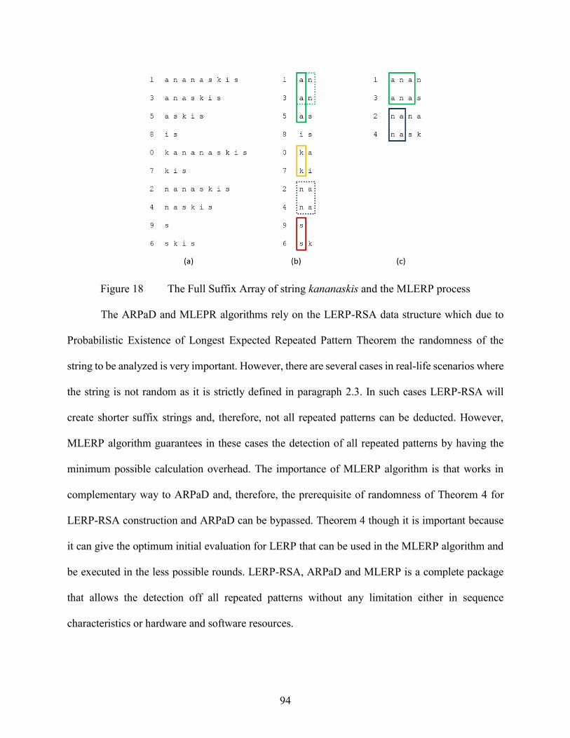
94

Figure 18 The Full Suffix Array of string kananaskis and the MLERP process

The ARPaD and MLEPR algorithms rely on the LERP-RSA data structure which due to

Probabilistic Existence of Longest Expected Repeated Pattern Theorem the randomness of the

string to be analyzed is very important. However, there are several cases in real-life scenarios where

the string is not random as it is strictly defined in paragraph 2.3. In such cases LERP-RSA will

create shorter suffix strings and, therefore, not all repeated patterns can be deducted. However,

MLERP algorithm guarantees in these cases the detection of all repeated patterns by having the

minimum possible calculation overhead. The importance of MLERP algorithm is that works in

complementary way to ARPaD and, therefore, the prerequisite of randomness of Theorem 4 for

LERP-RSA construction and ARPaD can be bypassed. Theorem 4 though it is important because

it can give the optimum initial evaluation for LERP that can be used in the MLERP algorithm and

be executed in the less possible rounds. LERP-RSA, ARPaD and MLERP is a complete package

that allows the detection off all repeated patterns without any limitation either in sequence

characteristics or hardware and software resources.

95

4.4.1 MLERP Algorithm Correction

MLERP Algorithm is based on the ARPaD algorithm. The proof of correctness is trivial.

Termination: MLERP algorithm is a looping execution of ARPaD algorithm, which has been

already proven to be finite. MLERP is also finite because it will repeat ARPaD at most 𝑙𝑜𝑔( 𝑛 − 1)

times. Therefore, MLERP will also terminate, as ARPaD does, and it is finite.

Correctness: Furthermore, MLERP is correct because in each loop ARPaD detects all repeated

patterns and MLRP recreates a new LERP-RSA for a new loop for the patterns found to have length

exactly equal to LERP. Therefore, since it has been proven that ARPaD terminates by finding all

repeated patterns, therefore, in each MLERP loop the new LERP-RSA contains less suffix strings

of different size, larger than the previously used LERP. Therefore, MLERP is also correct since

ARPaD has already proven to be correct.

4.4.2 MLERP Algorithm Analysis

For the MLERP algorithm the exact worst case complexity of the process depends on how

many iterations the MLERP algorithm requires, yet, there is no precise indication of these

repetitions (but definitely finite iterations of order 𝑙𝑜𝑔( 𝑛 − 1) in the worst case). In general, the

complexity of the whole process can be estimated first for the ORSAC algorithm as 𝑂(𝑛 + 𝑛 log 𝑛)

or 𝑂(𝑛 log 𝑛) if Merge-Sort is used. Then the MLERP algorithm has a while-loop that calls each

time the ARPaD algorithm. Although the whole process is definitely finite and can be finished in

very few steps (𝑙𝑜𝑔(𝑛 − 1)), it depends on the selection of the MLERP value and the size of the

sequence. In general, MLERP has log-linear complexity 𝑂(𝑛 log 𝑛) in the worst case or linear

𝑂(𝑛) on average. However, each time the while-loop ends the new 𝑛 value (in the complexity) is

significantly smaller than the original of the sequence because it represents the number of

96

occurrences found with length equal to LERP. Based on experimental results it can be observed

that the overall process is of type 𝑂(𝑛) in the average case or 𝑂(𝑛 log 𝑛) in worst case

[Xylogiannopoulos et al. 14b].

4.5 Single Pattern Detection (SPaD) Algorithm

As has been discussed in paragraph 2.2.3 several algorithms for pattern matching exist.

However, all these algorithms use Suffix Trees or Suffix Arrays with their variations. In this

paragraph, a novel algorithm for pattern detection will be presented which takes full advantage of

the LERP-RSA data structure. The superiority of the Single Pattern Detection (SPaD) algorithm

relies on the several important attributes of LERP-RSA and it will be proven that under specific

circumstances it can have constant time complexity 𝑂(1), which makes it unique in this category

of data mining.

Given a string 𝑆 of size |𝑆| = 𝑛 constructed from a finite alphabet 𝛴 and a pattern 𝑃 of size

|𝑃| = 𝑚, we need to search into S first, acknowledge the existence of P and if P exists then detect

the positions that P occurs in S. For this purpose, LERP-RSA will be used and binary search will

be applied directly to the data structure. Since LERP-RSA has to be constructed it is important to

identify the LERP value first. This is important because LERP is directly connected to P when

single pattern detection has to be applied. Depending on LERP two cases can be identified:

1) The length of P, |𝑃| is smaller or equal than LERP, |𝑃| ≤ 𝐿𝐸𝑅𝑃, or

2) The length of P, |𝑃| is greater than LERP, |𝑃| > 𝐿𝐸𝑅𝑃

The first case is trivial since if the length of P is smaller or equal to LERP it is only needed

to apply binary search in the appropriate class and return the results R of positions that P exists; if

P does not exist then R will be empty. Depending on the Classification Level which has been used,

97

binary search is executed in the class that P can exist based on the initial ordered digits of the

pattern and no further action is needed. Although the binary search algorithm with logarithmic

time complexity is used, yet, the process can be significantly faster than other algorithms because

the classes can be fractions of the original data structure due to classification.

The second and more complicated case is when the length of P is greater than LERP. In

this case pattern P will be partitioned in substrings each of which will be of length LERP at most.

In total ⌈𝑃

𝐿𝐸𝑅𝑃⌉ partitions of P can exist that will create a set of substrings 𝑆𝑃 = {𝑃1, 𝑃2, … , 𝑃𝑘},

where 2 ≤ 𝑘 ≤ ⌈𝑃

𝐿𝐸𝑅𝑃⌉ ∈ 𝑁∗ with |𝑆𝑃𝑖| = 𝐿𝐸𝑅𝑃 and having:

1) 𝑃1 starting at position 𝑃[1],

2) 𝑃2 starting at position 𝑃[1 + 𝐿𝐸𝑅𝑃],

…,

3) 𝑃𝑖 starting at position 𝑃[1 + (𝑖 − 1)𝐿𝐸𝑅𝑃], where 1 < 𝑖 < 𝑘,

…,

4) 𝑃𝑘−1 starting at position 𝑃[1 + (𝑘 − 2)𝐿𝐸𝑅𝑃] and finally

5) 𝑃𝑘 starting at position 𝑃[1 + |𝑃| − 𝐿𝐸𝑅𝑃].

It should be mentioned that the last partition will not consist of as many digits as the

remainder after the 𝑘 − 1 partition since we need to have size LERP. Having a size less than LERP

is not efficient because the last partition might be very small in size, e.g., have size one which will

cause the whole class to be returned as result. However, by making the last partition equal to size

LERP the aforementioned problem will be bypassed.

The next step after partitioning pattern P is to execute binary search for each partition in

the appropriate class and retrieve all positions at which each partition exists. The results will be a

98

set of vectors 𝑅𝑉 = {𝑅𝑉1, 𝑅𝑉2, … , 𝑅𝑉𝑘}, where 2 ≤ 𝑘 ≤ ⌈𝑃

𝐿𝐸𝑅𝑃⌉ ∈ 𝑁∗, one for each partition and

binary search execution in the corresponding class.

After the completion of binary search a check has to be executed on the positions in order

to determine if and where the original pattern P exists. First the Empty Bucket Criterion has to be

executed.

4.5.1 Empty Bucket Criterion

If any of the results vectors 𝑅𝑉𝑖 ∈ 𝑅𝑉 is empty then pattern P does not exist in S and the

algorithm terminates.

The validity of the above-mentioned criterion is obvious. Since pattern P has been split

into partitions, if even one of these partitions does not exist anywhere in string S then it is

impossible for pattern P to exist in S since part of it does exist in S:

𝐼𝑓 ∃ 𝑅𝑉𝑖 : |𝑅𝑉𝑖| = 0 ⇒ ∄ 𝑃 ∈ 𝑆

The Empty Bucket Criterion checks the trivial case when P does not exist and the algorithm

stops. However, if the criterion fails then pattern P may exist. In this case, first we sort all results

vectors and the Crossed Minimax Criterion has to be executed.

4.5.2 Crossed Minimax Criterion

If for any two continuous result vectors of result vectors set 𝑅𝑉𝑖, 𝑅𝑉𝑖+1 ∈ 𝑅𝑉, 𝑖 > 0 the

minimum value of the first plus LERP is greater than the maximum value of the second, or the

maximum value of the first plus LERP is smaller than the minimum value of the second, then

pattern P does not exist in S and the algorithm terminates:

99

𝐼𝑓 ∃ 𝑅𝑉𝑖, 𝑅𝑉𝑖+1 ∈ 𝑅𝑉 : {𝑚𝑖 𝑛(𝑅𝑉𝑖) + 𝐿𝐸𝑅𝑃 > 𝑚𝑎𝑥(𝑅𝑉𝑖+1)

⋁𝑚𝑎 𝑥(𝑅𝑉𝑖) + 𝐿𝐸𝑅𝑃 < 𝑚𝑖𝑛(𝑅𝑉𝑖+1)

⇒ ∄ 𝑃 ∈ 𝑆

The Crossed Minimax Criterion checks the case where there is a gap greater than LERP

between the results found for all partitions of pattern P. In this case, it is obvious that pattern P

cannot exist in string S. If Crossed Minimax Criterion fails, that means that pattern P may exist in

S and then algorithm continues execution.

At this point, there is a very important separation in the process that has to be made related

to the nature of the string S and if it is random or not:

4.5.3 String S is Random

Assuming that S is random then Theorem 4 guarantees that the longest expected repeated

pattern that can exist with high probability has length LERP at most. Therefore, it is expected that

each vector of the result vectors RV has one element at most. Since the Crossed Minimax Criterion

has failed, then pattern P exists in S and exists at the position of the first result vector 𝑟1 ∈ 𝑅𝑉1if

and only if for all continuous result vectors the difference between the elements of the result

vectors is exactly LERP, otherwise pattern P does not exist in S and the algorithm terminates:

𝐿𝐸𝑅𝑃 → ∀ 𝑅𝑉𝑖 → |𝑅𝑉𝑖| ≤ 1

𝐶𝑟𝑜𝑠𝑠𝑒𝑑 𝑀𝑖𝑛𝑖𝑚𝑎𝑥 𝐶𝑟𝑖𝑡𝑒𝑟𝑖𝑜𝑛⇒ |𝑅𝑉𝑖| = 1

and

𝐼𝑓 {

∀ 𝑟𝑖 ∈ 𝑅𝑉𝑖, 𝑟𝑖+1 ∈ 𝑅𝑉𝑖+1: 𝑟𝑖+1 − 𝑟𝑖 = 𝐿𝐸𝑅𝑃 ⇔ ∃ 𝑃 → 𝑟1 ∈ 𝑅𝑉1

∃ 𝑟𝑖 ∈ 𝑅𝑉𝑖, 𝑟𝑖+1 ∈ 𝑅𝑉𝑖+1: 𝑟𝑖+1 − 𝑟𝑖 ≠ 𝐿𝐸𝑅𝑃 ⇔ ∄ 𝑃

100

4.5.4 String S is not Random

If S is not random then Theorem 4 cannot be applied. However, it has been shown

experimentally in [Xylogiannopoulos et al. 16b] that approximately 95% of all repeated patterns

have length less than or equal to LERP. Therefore, if all partitions of P return results (more than

one for each result vector) then the results’ number per result vector is expected to be very small

compared to the size of S and all positions can be checked in order to detect all occurrences of

pattern P. There are two ways to perform this check.

4.5.4.1 Binary Search Check

The first method to check for all occurrences of P is by applying a direct binary search for

each result in the first result vector. If results found in the other results vectors that are multiples

of LERP, according to the results vectors’ indexes, then pattern P exists in the position checked in

the first result vector. If at least one case in any other result vectors exists which is not a multiple

of LERP related to the first results vector position, then pattern P does not exist at the specific

position and algorithm continues to the next instance in the first results vector. The process repeats

until all available positions in the first results vector have been checked:

∀ 𝑟𝑞 ∈ 𝑅𝑉1 → 𝐵𝑖𝑛𝑎𝑟𝑦 𝑆𝑒𝑎𝑟𝑐ℎ {

𝑟𝑞 + (𝑖 − 1)𝐿𝐸𝑅𝑃 , 𝑅𝑉𝑖<𝑘

𝑟𝑞 + (|𝑃| − 𝐿𝐸𝑅𝑃), 𝑅𝑉𝑘

⇒

𝐼𝑓 {

∃ 𝑟𝑖𝑞 ∈ 𝑅𝑉𝑖>1, 𝑟𝑖+1𝑞 ∈ 𝑅𝑉𝑖+1, ∀𝑅𝑉𝑖>1: 𝑟𝑖𝑞 − 𝑟𝑖+1𝑞 = 𝐿𝐸𝑅𝑃 ⇔ ∃ 𝑃 → 𝑟𝑞

∃𝑟𝑖𝑞 ∈ 𝑅𝑉𝑖>1, 𝑟𝑖+1𝑞 ∈ 𝑅𝑉𝑖+1, ∀𝑅𝑉𝑖>1: 𝑟𝑖𝑞 − 𝑟𝑖+1𝑞 ≠ 𝐿𝐸𝑅𝑃 ⇔ ∄ 𝑃

101

4.5.4.2 Linear Top Down Check

The second method to check all occurrences of P is by executing a linear top down check

in all results vectors “Figure 19”. Starting at the first result in results vectors 𝑟1,1 ∈ 𝑅𝑉1 the

algorithm starts to scan the second results vector 𝑅𝑉2 from the beginning for each one of the

positions in the vector and while the values are less than 𝑟1,1 + 𝐿𝐸𝑅𝑃. The following possible cases

exist:

1) The end of 𝑅𝑉2 has been reached and all positions are less than 𝑟1,1 + 𝐿𝐸𝑅𝑃. In this

case pattern P does not exist in S and the algorithm terminates.

2) A result found in 𝑟2,𝑖 ∈ 𝑅𝑉2 for which the value is greater than 𝑟1,1 + 𝐿𝐸𝑅𝑃. In this

case Pattern P could not exist in position 𝑟1,1 ∈ 𝑅𝑉1 and the algorithm continues to

result 𝑟1,2 ∈ 𝑅𝑉1. However, in this case the algorithm will not start from the

beginning of 𝑅𝑉2 but from the index where it has been stopped 𝑟2,𝑖 ∈ 𝑅𝑉2.

3) A result found 𝑟2,𝑖 ∈ 𝑅𝑉2 for which the value is exactly 𝑟1,1 + 𝐿𝐸𝑅𝑃. This is a valid

position for pattern P and in this case the algorithm will repeat the process between

the second and the third results vectors starting from position one in the third vector.

4) When all results in results vector 𝑅𝑉1 have been checked then algorithm terminates.

∀ 𝑟𝑞 ∈ 𝑅𝑉1 → 𝐿𝑖𝑛𝑒𝑎𝑟 𝑇𝑜𝑝 − 𝐷𝑜𝑤𝑛 {

𝑟𝑞 + (𝑖 − 1)𝐿𝐸𝑅𝑃 , 𝑅𝑉𝑖+1

𝑟𝑞 + (|𝑃| − 𝐿𝐸𝑅𝑃), 𝑅𝑉𝑘

⇒

𝐼𝑓 {

∃ 𝑟𝑖𝑞 ∈ 𝑅𝑉𝑖>1, 𝑟𝑖+1𝑞 ∈ 𝑅𝑉𝑖+1, ∀𝑅𝑉𝑖>1: 𝑟𝑖𝑞 − 𝑟𝑖+1𝑞 = 𝐿𝐸𝑅𝑃 ⇔ ∃ 𝑃 → 𝑟𝑞

∃𝑟𝑖𝑞 ∈ 𝑅𝑉𝑖>1, 𝑟𝑖+1𝑞 ∈ 𝑅𝑉𝑖+1, ∀𝑅𝑉𝑖>1: 𝑟𝑖𝑞 − 𝑟𝑖+1𝑞 ≠ 𝐿𝐸𝑅𝑃 ⇔ ∄ 𝑃

102

Figure 19 Linear Top Down Check Method

Both methods are very efficient. However, depending on the structure of the results one

may perform better than the other. For example, assuming that all results vectors have many

elements except the second which has only one, instead of performing binary search in all results

vectors the Linear Top Down Check may perform much better because it has only to check each

result from the first results vector to the one and only element of the second results vector before

it continues. However, in other cases Binary Search Check can perform better if each binary search

for results vectors is executed in parallel. There are many possibilities and combinations that can

be applied depending always on the nature of the results found.

4.5.5 SPaD Algorithm Correction

Termination: The SPaD Algorithm terminates despite if pattern P that has to be detected exists

or not. The first two criterions will check very fast if the pattern exists and if not they will stop the

process in order to avoid computation time to be lost. In case these two criterions will fail to detect

that pattern P does not exist, then there two cases:

103

1) String S is Random: in this case either pattern P exists if and only if for all

continuous results vector the difference between the elements of the results vectors

is exactly LERP and, therefore, SPaD will detect the pattern and terminate or

pattern P does not exist in S and the algorithm again terminates.

2) String S is not Random: in this case depending which method will be used the

following may happen:

a. Using Binary Check, SPaD will terminate when all results exist in the first

Results Vector will be checked against the rest of the Results Vectors and

b. Using Liner Top Down, SPaD will terminate when the results in each

Results Vector will be checked with the adjacent Results Vector.

Correctness: Correctness has been proven in paragraphs 4.5.1, 4.5.2, 4.5.3 and 4.5.4.

4.5.6 SPaD Algorithm Analysis

The computational complexity of the SPaD Algorithm it depends on the binary search

performed at the beginning of the execution in every class related to the subpatterns in order to

create the Results Vectors. The additional time needed in paragraphs 4.5.1, 4.5.2, 4.5.3 and 4.5.4

are almost not computable because they depend on the results found and not in the length of the

original string. Especially in the case of a random string (§ 4.5.3) the computational time is

constant and depends only on how many times the pattern is longer than LERP and, therefore, how

many Results Vectors exist.

Therefore, it is essential to focus only in the binary search of the initial execution of SPaD.

Although binary search has logarithmic complexity and it is expected that SPaD has exactly the

same logarithmic complexity 𝑂(log 𝑛), yet, it can be proved that SPaD can have actually constant

complexity 𝑂(1) or 𝑐, where c depends only on the size of the classes constructed for LERP-RSA:

104

For every subpattern that exists in the set of Sub Patterns binary search is executed and the

corresponding Results Vectors are created:

∀ 𝑆𝑃𝑖 ∈ 𝑆𝑃 → 𝐵𝑖𝑛𝑎𝑟𝑦 𝑆𝑒𝑎𝑟𝑐ℎ → 𝑅𝑉 = {𝑅𝑉1, 𝑅𝑉2, … , 𝑅𝑉𝑖, … , 𝑅𝑉𝑘}

From the definition of logarithm, we know that every real number can be expressed as

following:

∀ 𝑏, 𝑥 ∈ 𝑅∗, 𝑏 ≠ 1, ∃! 𝑦 ∈ 𝑅∗ : 𝑏𝑦 = 𝑥

𝑦 = log𝑏 𝑥

Therefore, for every finite alphabet the length 𝑛 of a string 𝑆 can be expressed as following:

∀ 𝛴: |𝛴| = 𝑚, |𝛴| ≠ 1, 𝑆: |𝑆| = 𝑛 ∈ 𝑁 ⊂ 𝑅∗, ∃! 𝑝 ∈ 𝑅∗ : |𝛴|𝑝 = 𝑛

𝑝 = log|𝛴| 𝑛

where floor of p is the String Power Factor (SPF) that will give the string length if the alphabet

will be raised in the power of the power factor. The maximum classification level it can be allowed

for LERP-RSA is:

⌊𝑝⌋ = ⌊log|𝛴| 𝑛⌋ → 𝑀𝑎𝑥𝑖𝑚𝑢𝑚 𝐶𝑙𝑎𝑠𝑠𝑖𝑓𝑖𝑐𝑎𝑡𝑖𝑜𝑛 ⇒⌊𝑝⌋ = 𝐿𝑚𝑎𝑥

𝐶𝑚𝑎𝑥 = 𝐶⌊log|𝛴| 𝑛⌋ = |𝛴|⌊log|𝛴| 𝑛⌋ = |𝛴|⌊𝑝⌋

where the cardinality (size) of each class, assuming equidistribution due to randomness required

for LERP-RSA, is:

|𝐶𝑚𝑎𝑥| =𝑛

𝐶𝑚𝑎𝑥=|𝛴|𝑝

|𝛴|⌊𝑝⌋= |𝛴|𝑝−⌊𝑝⌋ ≅ 1

Now it is essential to define the Classification Factor f as the difference between the

maximum number of classes we can have and the Classification Level has been used:

𝐶𝑓 → 𝐶𝑙𝑎𝑠𝑠𝑖𝑓𝑖𝑐𝑎𝑡𝑖𝑜𝑛 𝐹𝑎𝑐𝑡𝑜𝑟 𝑓 : 𝐿 = 𝐶𝑚𝑎𝑥 − 𝐶𝑓

and, therefore, each class can be expressed as:

105

𝐶𝐿 = 𝐶⌊𝑝⌋−𝐶𝑓 = |𝛴|⌊log|𝛴| 𝑛⌋−𝑓 = |𝛴|⌊𝑝⌋−𝑓

Based on the above the cardinality of each class is:

|𝐶𝐿| =𝑛

𝐶𝐿=

|𝛴|𝑝

|𝛴|⌊𝑝⌋−𝑓= |𝛴|𝑝−⌊𝑝⌋+𝑓 = |𝛴|𝑓𝑟𝑎𝑐(𝑝) + 𝑓, 𝑓𝑟𝑎𝑐(𝑝) ∈ [0,1)

where 𝑓𝑟𝑎𝑐(𝑝) is the decimal part of p.

Concluding, for the Binary Search we need:

𝐵𝑖𝑛𝑎𝑟𝑦 𝑆𝑒𝑎𝑟𝑐ℎ → 𝑙𝑜𝑔2|𝛴|𝑓𝑟𝑎𝑐(𝑝)+𝑓 = (𝑓𝑟𝑎𝑐(𝑝) + 𝑓) 𝑙𝑜𝑔2|𝛴|

calculations and, therefore, the complexity of SPaD algorithm is:

𝑂((𝑓𝑟𝑎𝑐(𝑝) + 𝑓) 𝑙𝑜𝑔2|𝛴|) → 𝑂(1) ∎

In brief the proof of constant complexity for the SPaD Algorithm claims that if the

Classification Level increases equivalently to the size of the string and, therefore, the number of

classes is increasing but the size of the classes is keeping the same, then Binary Search will have

to perform exactly the same steps, in the worst case, and, therefore, the complexity of the algorithm

with regard to the input size 𝑛 of the length of the string 𝑆 is always the same (constant).

4.6 Multiple Pattern Detection (MPaD) Algorithm

The Multiple Pattern Detection (MPaD) Algorithm is a direct application of the SPaD

Algorithm. More specifically, although the simple pattern matching problem refers to the detection

of a single specific pattern, the multiple patterns detection problem refers to the detection of a set

of patterns of equal size. Again, several algorithms exist, however, the combination of LERP-RSA

and SPaD produces a more efficient method because it allows memory and disk utilization while

it can also be executed on a set of different size patterns. The main difference is that instead of

searching one pattern after the other and, therefore, having to load several classes in memory and

106

possibly repeat the process for classes already processed, a pre-process analysis can perform more

efficiently:

1) All patterns have to be partitioned, as explained in previous paragraph for the SPaD.

2) The substrings produced in (1) will be grouped based on the Classification Level

of LERP-RSA, i.e., based on the order first digits.

3) For each group of substrings SPaD will be executed and the results vectors will be

stored in an array. This array is the array of the results vectors RVA.

Then SPaD algorithm is executed for each one of the substrings of the RVA until all of

them have been checked for existence and detected or not. The proposed methodology is very

efficient for the following reasons:

1) It minimizes the disk access because each class that has to be checked for each

group of substrings is loaded on memory only once. Because of this the overall

process can be significantly accelerated since the most time-consuming part of

pattern detection algorithms is disk I/O access.

2) There is no need for the initial patterns to be of equal size. MPaD can be executed

on completely different sizes patterns.

3) MPaD is based on SPaD execution and, therefore, has binary search as a backbone

which is extremely fast.

4) Moreover, due to use of classification for the LERP-RSA the classes are smaller

compared to the original string S and, therefore, binary search can be executed

much faster.

107

4.7 SPaD and MPaD Wildcards Pattern Detection

Both SPaD and MPaD can be executed using wildcards. Although the process is exactly

the same as described in previous paragraphs for SPaD and MPaD, the only differentiation is on

the number of results SPaD will return. Indeed, searching in a class for a substring of the pattern,

a wildcard binary search, will return many more results due to the wildcard character. In this case,

the Results Vectors that will be created will be significantly larger and eventually more time will

be needed for the data mining, yet, it is insignificant compared to the initial string S in which

pattern detection is executed.

Instead of using SPaD with already existing wildcard pattern detection algorithms, another

direct approach is to break down the patterns based on the wildcards occurrences and, therefore,

transform a single pattern detection problem of SPaD to a multiple patterns detection problem of

MPaD. Again, the complexity depends on the number of results which will be returned by the

Results Vectors.

4.8 Multivariate or Multidimensional Pattern Detection (MvdPaD)

SPaD, MPaD and ARPaD algorithms can be used not only to search for single, multiple

and all repeated patterns in single dimension sequences but also in multidimensional sequences or

multivariate systems of sequences. Moreover, MvdPaD process described below allows the

analysis of strings of different lengths which is a great advantage of the method and can be used

for clickstream or transactions analysis, financial time series when multiple series from different

values have to be analyzed for correlation detection such as a stock behaviour against an index,

weather analysis when many different parameters have to be analyzed for forecasting purposes

such as air temperature, air humidity, air speed and many more. In the case of multidimensional

analysis, a trivial example is the pattern detection in images where an image of size 𝑛×𝑘 can be

108

split in 𝑛 row strings of length 𝑘 or, equivalent, to in 𝑘 column strings of length 𝑛 and perform the

pattern detection.

MvdPaD has two distinct phases of execution based on LERP-RSA and ARPaD or any

other of the SPaD and MPaD algorithms. The only prerequisite of the MvdPaD is that all sequences

have been constructed from the same alphabet. In case they are not, then a new alphabet has to be

constructed, which is the concatenation of all alphabets without repetition of common alphabet

characters. Then the following process can be applied for single, multiple and all repeated patterns

detection:

1) For each string the corresponding LERP-RSA is created,

2) All LERP-RSA are combined together in a larger LERP-RSA data structure,

3) The new LERP-RSA is lexicographically sorted and

4) SPaD, MPaD and ARPaD algorithms are executed on the new LERP-RSA

depending on the nature of the pattern detection.

Although with the use of the new, combined and enlarged LERP-RSA it could be claimed

that information is lost, this is not the case. There are several ways to combine the partial LERP-

RSA constructed for each string initially. One way is to add the string index as a new attribute.

This can lead to the use of one more field of the LERP-RSA, yet, it will be considerably small in

size since with a single byte integer we can have up to 256 strings while with a two-byte integer

we can have up to 65,536 strings. If saving space is very important then the following approach

can be used. Assuming that the longest string 𝑆𝑘 has length 𝑛𝑘 then we assign different position

index numbering to strings based on, e.g., the decimal power which is larger than 𝑛𝑘. For example,

if we have three strings of length 100,000, 750,000 and 2,500,000 characters then we can use a

107 ten million numbering system and the first-string positions will start at 0 and end at 99,999,

109

the second will start at 10,000,000 and end at 10,749,999 while the third will start at 20,000,000

and end at 22,499,999. This allows having a constant gap between the strings which further allows

easy calculation of absolute positions inside each one of them by a simple subtraction.

The whole process is very simple and one of the approaches will be presented in detail with

the experiment of paragraph 5.5 where a transactions analysis will be performed. It is just a smart

reconstruction of the LERP-RSA which allows any other algorithm to be executed simultaneously

on all strings.

111

Chapter 5 Testing and Verification in Diverse Scientific and Commercial Fields

5.1 Introduction

In the current chapter, several different types of applications are covered. It will be

presented how LERP-RSA and ARPaD can be used to solve important, yet, very difficult in some

cases, problems in diverse scientific and industry fields such as (a) event and time series analysis,

(b) bioinformatics, (c) network security, (d) multivariate sequences analysis, (e) clickstream

analysis, (f) real time data stream analysis, (g) mathematics, (h) image analysis, (i) compression

and, finally, (j) text mining. Specifically, for the mathematical area of interest the focus is on

Number Theory and Normal Numbers. The last of the experiments has been conducted on the first

trillion (1012) digits of the decimal expansion of π and it will prove that for this length π is a normal

number. This also proves the novelty and flexibility of LERP-RSA to solve problems when the

available hardware and software resources are extremely limited compared to the problem size and

requirements.

The applications presented here are not the only ones that exist. They have been used more

to demonstrate the great spectrum of application of the proposed methodology in the current thesis.

Moreover, the applications of the next paragraphs will illustrate the flexibility of LERP-RSA data

structure and the importance of the unique ARPaD algorithm by proposing solutions to several

dissimilar problems through the detection of all repeated patterns.

Part of the material covered in this chapter has been published in fully refereed journals

or presented in conferences and published in the corresponding proceedings [Xylogiannopoulos

et al. 14a, 14b, 14c, 15b, 16a, 16b, 16c].

112

5.2 Event Series and Time Series Analysis

Event Series and Time Series analysis from a data mining perspective are equivalent. While

an Event Series is any series of distinct events of the same category, in a Time Series the parameter

of time for each event observation has been added. However, the only distinction between these

two types of series is the ordering parameter which can be either generic by using an index, e.g.,

1, 2, 3, … describing a series of earthquakes which happened in a specific region, or it can be

specific to time and describing, e.g., daily stock prices. In the second case the time interval can

also vary depending on the variable under analysis. For example, stock prices can be analyzed

using daily closing prices, yet, can also be analyzed using intraday per second prices. Furthermore,

weather data can also be analyzed using daily intervals while geological events can be analyzed

using as a time interval centuries or millenniums. Nevertheless, pattern detection can be applied

in all cases detecting repeated patterns based on LERP-RSA and ARPaD. The only difference

between the discovered results is that for an Event Series the positions of each pattern are irrelevant

to time, i.e., the patterns are important in relation to each other in the sequence of events, while in

a Time Series the positions are directly correlated to absolute time.

The detection of all repeated patterns is a very important aspect of Event and Time Series

analysis. The results can be used to be analyzed by periodicity detection algorithms and further

detect either correlation between patterns or repetition of patterns with a specific interval (period),

e.g., two different patterns occur with a gap between each other of 30 data points or a single pattern

occurs every 50 data points. In this case it can be assumed, according to the confidence of the

periodic occurrences, that these patterns are expected to occur again in the future and, therefore,

used for forecasting purposes in, e.g., weather data, financial data, seismic waves, traffic control

etc.

113

The pattern detection analysis for forecasting purposes will be presented here using data

from the Dow Jones Industrial Average 30 Volatility Index (VXD). The specific index calculates

the volatility of one of the most well-known and important indexes in the US stock market, Dow

Jones Industrial Average 30 (DJIA30). VXD is a very important index because the derivative

market is based upon it, since volatility is one of the key-major factors in calculating derivative

prices. Derivative exchanges especially in the US are considered to be a market of hundreds of

trillions of dollars. Therefore, it is of great importance to check if there are any patterns that might

have periodicity with great confidence, which can be used for forecasting purposes in order to detect

or prevent anomalies in the stock market.

The volatility of a stock (or any underlying variable such as an index) is a measure regarding

analysts’ uncertainty about the returns a stock might provide and can be defined as the standard

deviation of the return provided by the stock in one year period when this return is expressed using

continuous compounding [Hull 12]. Volatility is very important to be calculated because it is one

of the many factors like gamma, delta, theta, vega etc. that derivative functions and models use to

calculate the fair price of derivatives like futures, options, forwards etc. Especially in the case of

options, in the Black-Scholes-Merton pricing formulae, the most important factor is volatility and

it is actually the one that cannot be directly observed and, therefore, analysts usually use the implied

volatility [Bodie et al. 10, Hull 12]. Indexes usually represent stock markets or they can represent

specific industry groups or different capitalization companies. In every case a mathematical formula

has been used to express either an industry group or the whole stock market in the best possible

way by taking into consideration specific attributes of the underlying variables which are listed

companies. Therefore, it is important to remember that since VXD index that will be analyzed here

is populated upon actual prices of the standard DJIA30 index, it follows the same chaotic model.

114

In the particular experiment, daily data will be used and discretized based on an alphabet of

four letters {𝐴𝐵𝐶𝐷} representing quartile classification of the data. The calculation of the data

values for the VXD index is based on records taken from YAHOO! financial website [YAHOO!

12] and the time horizon is from 1971 till 2010, covering forty years of observations or creating a

time series of exactly 10,074 data points.

The first step in the process is to create the time series strings based on the discretization

method. After the time series string creation, the creation of LERP-RSA follows. The next step is

the calculation of all the patterns that are candidates for periodicity using ARPaD algorithm, i.e.,

all repeated patterns. The calculation of all patterns with period equal or greater than two is needed.

Although two occurrences do not establish a periodicity by themselves, it is important for them to

be calculated in the event that the next expected occurrence will appear outside the time series

boundaries, which is in the future. That means that if the space between the two occurrences

(actually the period) is longer than the remaining length between the second occurrence and the end

of the times series, sometime in the future a third occurrence is expected to occur, if the periodicity

is valid. However, such occasions can only be validated in a future time by the actual facts. The last

step is the analysis of the results produced by ARPaD. It is important to identify patterns that show

some kind of periodicity and for this purpose Periodicity Detection Algorithms from [Rasheed et

al., 10] have been used. For the Periodicity Detection Algorithms, 75% has been used as a

confidence limit in order to have results that are meaningful. For example, if a pattern has perfect

periodicity twenty and only two occurrences, ARPaD will report it as a repeated pattern. However,

for forecasting purposes it is not important since it has confidence just 10 percent. For this reason,

the confidence has been set to equal or greater than 75% in order to get back as many reliable

outcomes as possible.

115

After the periodicity detection, the indicative results presented in Table 1 show some very

long patterns (substrings) constructed by one letter, i.e., 35 characters long with “A”, 34 characters

long with “D” and 52 characters long with “D”. All these long strings represent several weeks of

standard, unchanged levels of volatility. This is important since it means that the prices of options

in the Black-Scholes-Merton pricing formula will have rather stable values for a significant period

of time. Nevertheless, in the cases of the “D” strings it is very important for the derivatives since it

implies high volatility for a long period of time, despite the fact that this volatility was kept high

for a significant period of time. Further examination is needed since financial or political factors

might have influenced financial markets for a long period and, therefore, kept the volatility high.

However, the specific samples do not have many occurrences. They can be found only three times

in the time series but what is really important is the fact that the longest pattern of “D” has

confidence one which means perfect repetition. What is more interesting is that if we check the

actual positions in calendar time, i.e., between 1970 and 2010, the first occurrence identifies the

financial collapse of the US stock market in October 1987 when Black Monday occurred on

Monday, October 19th, which resulted in the collapse of DJIA30 by 22.61%. The second event is

related to the financial crisis in August 1998 due to the Russian currency collapse and the Long-

Term Capital Management Hedge Fund crisis that led to its final bankruptcy. Finally, the third event

is the most recent financial crisis melt down in March 2009 due to the very well-known liquidity

crisis in the banking system and the aftermath of the Lehman Brothers Investment Bank bankruptcy

that took place in September 2008. Moreover, several shorter patterns (substrings) have been found

with good confidence indicating that there is some kind of periodicity.

116

Table 1 Indicative Data Results for Quartiles with Confidence Greater or Equal Than 0.75

Pattern Starting

Position Period

Occur-

rences

Confidence

Level

AAAAAAAAAAAAA 7,476 750 3 0.75

AAAAAAAAAAAAAA 6,521 954 3 0.75

AAAAAAAAAAAAAAAAAAAAAAAAAAAA

AAAAAAA 3,710 1,669 3 0.75

AAAAAAAAAAAAAAAAAAAAAAAAAAAA

AAAAABBBBBB 1,376 2,202 3 0.75

BBBAAAA 6,457 1,010 3 0.75

BBBBAAAA 7,466 751 3 0.75

BBBBBBBBBBCCCCCC 8,357 839 3 1.00

BBBBBCCCCCC 8,921 280 4 0.80

BBBBBCCCCCCCCCCCCCC 8,362 559 3 0.75

CCCCCCCCCCC 9,399 326 3 1.00

CCDDDDD 4,965 1,381 3 0.75

DDDDDDD 9,849 56 3 0.75

DDDDDDDDDDDDDDDDDDDDDDDDDDDD

DDDDDD 4,969 1,649 3 0.75

DDDDDDDDDDDDDDDDDDDDDDDDDDDD

DDDDDDDDDDDDDDDDDDDDDDDD 4,258 2,691 3 1.00

5.3 Bioinformatics

As has been mentioned in previous paragraphs, LERP-RSA requires a good estimation of

the LERP value based on the Probabilistic Existence of Longest Expected Repeated Pattern

Theorem, while the Theorem asks for the sequence to be random, i.e., normal. DNA, RNA, gene

and any other types of strings used in bioinformatics are not expected to be random for several

reasons that have to do with the nature of live organizations. This fact can also be observed from

the experimental results regarding the occurrences’ lengths of chromosome 9 from the human

genome as they are published in [Xylogiannopoulos et al. 16b]. The data for these experiments

have been provided by the University of California Santa Cruz Genome Bioinformatics and the

human chromosome 9 has been used. For the current experiments a standard personal computer

with double core Intel Core2 CPU at 2.2 GHz with 1 thread per core, 4 GB of RAM, 80 GB of hard

117

disk space and 32bit operating system has been used. Microsoft SQL Server 2008 has also been

used to support the analysis.

Two experiments are presented with strings of length 2 million and 4 million characters.

Although Mean seems to have some kind of normality and increases as expected, all other

parameters of dispersion are very extreme (Table 2). Standard Deviation is above 10 as it is the

coefficient of Skewness (around 15) and the coefficient of Kurtosis takes very extreme values

approximately between 300 and 400. Moreover, although the third Quartile is very low, meaning

that 75% of the observations are below 13 for the string of length 4 million characters, yet, the

longest occurring pattern has size 548 characters, which is the same in both cases. This outcome

means that at the specific part of the DNA string which has been analyzed, for a particular reason a

long pattern of 548 letters repeats at specific positions in the string (Table 3). This result can be

further analyzed by biologists to examine why this happens. Furthermore, the detection of all

repeated patterns can be potentially very useful for detecting protein receptors or other parts of the

DNA sequence in order to understand how different, yet, similar parts of DNA are correlated.

Again, this methodology is a tool that can be used by biologists who are experts in this field in order

to decrypt and demystify the results.

All these outcomes demonstrate that the DNA strings do not follow a specific known

distribution and do not satisfy Theorem 4, Preposition 1 and Lemma 4. In fact, all hypotheses testing

conducted (trying to fit the distribution of the DNA experiments occurrences’ lengths to any

distribution) have been rejected for all known distributions “Figure 20” and “Figure 21”. As

expected, the fact that DNA strings are not random, they failed to comply with the prerequisite of

Theorem 4, Preposition 1 and Lemma 4. However, what is very optimistic is the fact that despite

the failure, the actual longest repeated pattern seems to be very small compared to the size of the

118

string. Further, the theoretical LERP discovers more than 95% of all repeated substrings. Repeated

substrings that have lengths greater than the theoretical LERP are very few and, therefore, the

proposed approach can be applied as it is if we care to discover the great majority of the occurrences

with normal lengths. In this case, the method can be used to create a very small suffix array in

accordance with the purpose of the LERP methodology. Even if all repeated susbtrings are needed

to be found, the MLERP process can be executed with the theoretical LERP as initial value in order

to discover all patterns. Using LERP as initial value for MLERP will allow a fast discovery of all

repeated patterns since the LERP value is the optimum value for starting the MLREP process. In

the current experiments with the DNA, MLERP can be executed with a LERP value for the second

phase of 25 times the initial value (i.e., 600 or 625) and can complete the analysis in just two steps.

It is important to mention that although ARPaD discovered more than 2 million patterns in

a few minutes, yet, other algorithms used for single pattern detection need approximately the same

time to discover one pattern [Parker 09] with the use of suffix trees. Furthermore, in [Parker 09]

only chromosome 21 was analyzed using an Intel Xeon 8 core CPU at 3.00 GHz with 31GB RAM

and although chromosome 21 is the shortest in human DNA sequence with length approximately

33 million characters (cleaned) and despite the considerable superior hardware resources “when the

whole chromosome was tested, there were some memory problems and the program would run very

slow.” (p. 22) [Parker 09] Although in the current DNA experiments the whole chromosome has

not been tested, yet, as will be presented in the next paragraphs, the analysis of sequences of length

billions of characters can be executed with fewer resources compared to [Parker 09] and get the

results very fast without facing memory limitations due to the superiority of LERP-RSA compared

to suffix trees.

119

Table 2 Location, Dispersion and Shape Parameters for DNA string experiments

String

Length (n) Q1 Q2 Q3 Mean

Standard

Deviation Skewness Kurtosis

2,000,000 10 11 12 13.26 15.97 15.38 313.24

4,000,000 11 12 13 14.37 14.63 16.28 408.52

Table 3 Theoretical and Actual LERP for DNA Strings Experiments

String

Length (n) 𝐏(𝐗)

Alphabet

(m)

Theoretical

LERP

Actual Longest

Repeated Pattern

2,000,000 0.01 4 24 548

4,000,000 0.01 4 25 548

Figure 20 Occurrences per pattern length and Cumulative Occurrences for DNA experiment

with length n=2,000,000

120

Figure 21 Occurrences per pattern length and Cumulative Occurrences for DNA experiment

with length n=4,000,000

The detection of all repeated patterns may not seem very useful in bioinformatics but on

the contrary it can be proven to be of extreme importance in many cases. For example, it can be

used for Tandem Repeats detection in DNA strings. A Tandem Repeat is two or more adjacent,

exact or approximate, repetitions of a pattern of nucleotides. Although several algorithms and tools

exist for tandem repeats detection these are fast only for small DNA strings and pattern sizes.

However, with the use of ARPaD and the detection of every possible repeated pattern in a DNA

string we have the limitless potential to perform any kind of meta-analyses in the results of the

algorithm and detect any kind of tandem repeats very fast.

Another very important application of all repeated patterns detection in bioinformatics is

sequence alignment. Sequence alignment in bioinformatics is a way of arranging two or more

sequences of DNA, RNA or protein in order to detect sections of similarity. This problem is very

important and very difficult and was addressed firstly by Needleman and Wunsch [Needleman and

Wunsch 70] who introduced one of the first dynamic programming algorithms for global sequence

121

alignment. Another algorithm for local sequence alignment was introduced by Smith and

Waterman [Smith and Waterman 81]. However, the use of dynamic programming for sequence

alignment is not very efficient and faces difficulties since it cannot scale up in order to be used for

very long sequences.

In contrast, the ARPaD algorithm can be used to propose a solution for this problem in a

more efficient way. Assuming that we have two (or more) sequences that we want to align, we can

use the ARPaD to detect all repeated patterns between the sequences. We can filter the results to

include repeated patterns between the sequences but not repeated patterns that exist inside the same

sequence. Then, we have to sort the patterns based on their length and the smallest difference

between their positions by introducing a new attribute, the Position Difference Index (PDI). For

example, if a pattern occurs in one sequence at position 5 and in another sequence at position 7,

then the PDI is 2. Sorting patterns by the smallest PDI allows us to know what patterns occur in

exactly the same position in both sequences and, therefore, are already aligned. After finishing

with patterns with PDI 0, we can continue with patterns with larger PDIs until we produce the best

possible alignment. The PDI index can also be defined as the alignment error for patterns between

different sequences. Using this methodology allows us to achieve one of the best possible sequence

alignments.

5.4 Network Security

The rapid growth of electronic devices has transformed the Internet into a significant means

of communication all over the world. Because of this, the Internet has experienced an exponential

growth in users, services and solutions provided by many public and private organizations. This

growth has also led to an increase in different types of cyber threats and crimes. One of the most

122

frequent and detrimental effects is the Distributed Denial of Service (DDoS) attack, with which

someone can unleash a massive attack of communication requests through many different isolated

hosts and cause a system to become unresponsive due to resources exhaustion. The significance

of the problem can be easily acknowledged due to the large number of cases regarding attacks on

institutions and enterprises of any size which have been revealed and published in the past few

years.

In this paragraph, a novel method is introduced, which is based on LERP-RSA and ARPaD

algorithm and published in [Xylogiannopoulos et al. 16a], that can detect all repeated patterns and,

therefore, analyze incoming IP traffic details and warn the network administrator about a

potentially developing DDoS attack. In a DDoS attack case, the algorithm can analyze all IP

prefixes and warn the network administrator if a potential DDoS attack is under development based

on the detection of suspicious IP addresses and their analysis depending on pre-set thresholds on

a variety of parameters such as maximum allowed IPs per country, per minute, etc. Moreover, this

analysis provides useful information, such as geolocation of incoming traffic, and gives the ability

to the network administrator to block, manually or automatically, potential groups of IPs that can

be categorized as suspicious, while allowing legitimate users to continue their work. Based on the

experiments conducted on real data from the Centre for Applied Internet Data Analysis

organization [CAIDA 08] which will be presented here, it has been proven experimentally how

rapidly an alert can be raised for a potential DDoS attack. Therefore, the method introduced can

identify and detect a potential DDoS attack while it is being initiated and before it has detrimental

effects on system resources. Furthermore, a system based on this method can scale up depending

on the needs of any organization, from a small e-commerce company to large public or private

institutions, by providing the same level of high performance detection.

123

In order to analyze the incoming traffic as faster as possible, all advanced attributes of

LERP-RSA data structure will be used that allow the parallel execution of the ARPaD over each

class and, therefore, the significant acceleration of the analysis. However, the use of LERP-RSA

data structure requires major transformations to the methodology originally presented in

[Xylogiannopoulos et al. 14c]. More specifically, the recording of IP addresses as exist in the IPv4

protocol does not allow us to take full advantage of the LERP-RSA because only 3 classes can be

created based on the decimal system, i.e., IP address strings starting with 0, 1 and 2. Actually the

last class sample space is significantly smaller since it can take values up to 255 only and not up

to 299. Due to the small number of classes, the improvement is not significant. In order to take full

advantage of the classification, whenever a new packet arrives, instead of using the decimal

representation of IPv4 address, each octet of the address has to be converted to the hexadecimal

equivalent, e.g., IP address 123.45.6.78 will be transformed to 7B.2D.6.4E and the corresponding

string will be 7B2D064E. Doing this, two significant improvements have been achieved:

1) The length of IP address string is no longer 12 but 8, which is 1/3 smaller and will

help towards a faster analysis of the IP addresses list and

2) Since the values of the octets have changed from 0-255 to 00-FF this means that

LERP-RSA data structure can be classified using hexadecimal system and create

16 classes which can cover the whole sample space of possible octets.

Another important aspect of the transformation in (2) is that it allows the execution over the new

IPv6 protocol directly, with the new addressing scheme. The only change that has to take place is

to transform every empty octet “::” to double zeros, i.e., “:00:” and remove colons when importing

the strings in LERP-RSA.

124

After the creation of classes, the next step is to lexicographically sort each one based on

the IP address string. The last step is to execute the ARPaD in parallel over each one of the 16

classes. This can significantly decrease the overall time needed and assuming that all classes are

equal-distributed can be of a magnitude of more than 1/16 of the time needed in the originally

proposed method [Xylogiannopoulos et al. 14c], taking also into consideration the smaller string

sizes that have to be analysed in this case.

This analysis can return every IP that occurs at least twice in the IP list. Yet, the Network

Administrator can set different parameters and thresholds, which can be either static or dynamic,

and raise a warning signal for a potential DDoS attack. The analysis can be performed following

different schemes:

1) Using a fixed time interval analysis at which the IP addresses are collected and

analyzed at every specific timespan, e.g., 1 minute, 5 minutes etc.,

2) Using a fixed number of packets, e.g., 100,000 for which whenever the specific

number of packets has been collected, can be analyzed regardless of the timespan

they occurred and/or

3) A combination of the above where the Network Administrator can set a criterion to

execute the analysis based on which threshold is met first (time or packets).

All these parameterizations depend on the hardware and bandwidth available to the infrastructure

used and can be determined and adjusted dynamically by the Network Administrator.

The completion of the IP addresses analysis will initiate the detection phase which will

identify potential threats based on a set of custom variables, set by the Administrator. Additionally,

it is possible to directly identify to whom a domain or host IP belongs which can allow Network

Administrator to decide if this can be a suspicious traffic that can lead to a DDoS attack. This

125

information can be provided in real time to the Network Administrator who can decide to block

the communication in the level of hosts, domains, countries or geographical regions from accessing

the network resources and allow legitimate users to continue using the services without

experiencing any degradation.

For the experiments a personal computer with an Intel i7 quad core processor and 16GB

RAM has been used. The code of the ARPaD algorithm has been written in C# and a 64bit

operating system has been used. The dataset used in the experiments comes from the CAIDA

organization and is the DDoS attack [CAIDA 08] covering approximately one hour of traffic in a

time span from August 4, 2007, 20:50:08 UTC to 21:56:16 UTC. As it is stated on CAIDA website

[CAIDA 08] “non-attack traffic has as much as possible been removed.” The experiment is

executed in 34 rounds, one for each minute of the dataset, covering most of the attack time span.

Also, sixteen threads are used to analyse in parallel each class in four phases each one for each IP

prefix and IP prefix strings phases executed sequentially, i.e., 00.xx.xx.xx, 00.00.xx.xx,

00.00.00.xx and 00.00.00.00, due to hardware limitations. Depending on the hardware and

resources availability, all the threads can be executed in parallel, something which although can

give incredibly low processing time it also means that 64 threads should run in parallel.

126

Figure 22 CAIDA DDoS attack from August 4, 2007, 21:50:08 UTC to 21:23:59 UTC

dataset LERP-RSA and ARPaD execution in four phases

As can be observed in “Figure 22” the execution time of LERP-RSA and ARPaD is

significantly faster than the attack, approximately 15 seconds for each minute of the DDoS attack.

In these 15 seconds of execution time in most of the cases more than nine million IP addresses

have been analyzed. For the 18 minutes of the DDoS attack, with more than 162 million packets,

less than 4 minutes of execution time has been needed for LERP-RSA and ARPaD.

5.5 Transactions Analysis

Detecting frequent itemsets is one of the most important problems of data mining addressed

firstly by Agrawal and Srikant [Agrawal and Srikant 95]. Sequential frequent itemsets detection as

introduced in [Agrawal and Srikant 95] is a special case of the general problem of detecting

sequential itemsets and it will be discussed here due to many fields of implementation it has in, e.g.,

business, marketing, finance, insurance etc., based on the thorough analysis it has been presented

127

in [Xylogiannopoulos et al. 16c]. For example, sequential frequent itemsets detection can be used

when we want to examine how frequently “a new car is bought and a new insurance policy is bought

immediately after the car.” A more representative example of sequential itemsets (or patterns)

detection can be derived from the car industry as follows: Whenever a car is sold, the owner has to

go through a service process which can include, e.g., engine oil change, tires change, brakes fluid

change, service after 100,000 km etc. In this sequence of events an engine or any other part of the

car may fail. The car industry is very interested in detecting when a failure occurs in the sequence

of service events, in order to reform the timeline of services or make specific parts more durable

etc. In the above mentioned example the order of events is essential. It is completely different to

say “oil change, brake fluid change” than “brake fluid change, oil change.” That is an illustrative

definition of sequential itemsets, assuming that each event is an item. Moreover, each event in the

above-mentioned example, or generally speaking each item, can reoccur, such as oil change.

The problem of sequential frequent itemsets detection is also very similar to the problem of

detecting repeated patterns in time series. In such a case, we have a very long string of discreet

values based on a predefined alphabet and we want to detect patterns that exist in the string (e.g.,

in DNA). Yet, in the general case of sequential frequent itemsets detection, we have transactions

constructed from items and we want to detect sequential itemsets that exist in more than one

transaction. Common methods to address the specific problem are to either use apriori type, pattern

growth type or hybrid type algorithms while lately, hybrid and early pruning algorithms have been

also presented that can address the specific problem adequately [Agrawal and Srikant 95, Masseglia

et al. 98, Garofalakis et al. 99, Ayres et al. 02, Yang et al. 07, Mabroukeh and Ezeife 10].

In the current thesis, the general problem will be addressed as it will be defined here and

not as it is defined by Agrawal and Srikant in [Agrawal and Srikant 95]. More particularly, in

128

[Agrawal and Srikant 95] an itemset is defined as “a non-empty set of items.” (p.3) Yet, it is

important to mention that the specific definition does not conform to the strict mathematical

definition of a set, as it derives from Set Theory. In Set Theory, “a set is formally defined to be a

collection of distinct elements.” [Akerkar and Akerkar 07] Furthermore, a sequence is an ordered

collection of objects for which reoccurrence is allowed. Since in data mining, for pattern detection

purposes, we care about sequences where their objects can reoccur, we can also accept this for

collections of items by strictly stating the deviation from the mathematical definition. We can allow

an item to occur more than once in an itemset e.g., the DNA sequence can also be considered a set

of proteins constructed from alphabet {A, C, G, T} where every arrangement of proteins (patterns)

can also reoccur in the DNA sequence. Therefore, in order to be accurate, we have to redefine

itemset, for data mining purposes, as a collection of items where the reoccurrence of each item is

allowed, while the detection of sequential itemsets can be defined as the detection of ordered

itemsets in a sequence, for which the repetition of an item is allowed.

Therefore, we can redefine the sequential itemsets detection problem as the detection of

itemsets (as defined above) which can occur either in the same sequence (also expressed as

transaction) and/or in different sequences in a collection of sequences. The above definition is the

generic definition of the problem because we cover every possible combination of itemsets

detection, i.e., (a) single item itemsets (e.g., having only one element, where of course ordering

cannot be directly defined), (b) itemsets containing a whole sequence of items, (c) itemsets that

appear only in different sequences, (d) itemsets that appear multiple times in the same sequence and

finally (e) itemsets that can occur in the same sequence and/or in different sequences.

In order to address the problem of detecting sequential frequent itemsets, LERP-RSA and

ARPaD will be used for the detection of all repeated patterns. The proposed methodology allows

129

the detection of not only the most frequent sequential itemsets but all itemsets that exist at least

twice in a database of transactions. The novelty of the proposed methodology is based on two

factors:

1) It can rapidly detect every sequential itemset and

2) The detection can be done regardless of any kind of support threshold.

As has been already shown in [Xylogiannopoulos et al. 16b] the detection of every repeated pattern

can take on average less than 0.2 milliseconds and therefore even when thousands of patterns have

to be detected the overall time is not a significant problem. Moreover, although the detection of

every sequential itemset, and, therefore, itemsets of very low frequency, seems insignificant, in

some cases this can be proven to be very useful especially when outliers are detected e.g., in the

case of fraud detection, anti-terrorism surveillance and analysis, etc. Furthermore, by performing

the specific analysis periodically we can detect trends in low frequency itemsets which may

increase/decrease slower or faster and thus lead to appropriate actions, e.g., in developing different

marketing policies and strategies. Alternatively, the proposed methodology can also be used to

specifically detect low frequency itemsets, something that, to the best of my knowledge, does not

exist in literature.

As has been discussed in previous chapters, the method to detect all repeated patterns can

be summarized as follows:

1) First all suffix strings are created from the original string and then they are

lexicographically sorted and

2) After the data structure creation phase ARPaD algorithm runs and detects all

repeated patterns that exist at least twice in the string.

130

If each transaction is considered as a string, then the same process can be followed to create

the suffix array for the specific transaction. Of course, in just one transaction any repeated pattern

cannot be detected (itemset in our case) because it simply does not exist. In order to have any kind

of repetition in a single transaction repeated items have to exist. Usually this is not the case despite

the fact that there are times when this may occur, e.g., recording webpage visits by users when in a

single session a user may go back and forth and repeat the same webpage visiting process on a

website. In this example, ARPaD algorithm will detect these repeated patterns (itemsets). However,

in general it is important to find frequent itemsets among different transactions. In this case, we can

create a LERP-RSA for each transaction and then combine all LERP-RSAs together. Then ARPaD

algorithm can detect all repeated patterns (itemsets) among all transactions, which have been

inserted into the database.

Usually all other methods for sequential frequent itemsets detection follow a two-phase

process. First, the transactions are entered in the database and then an algorithm scans the database

to detect the sequential frequent itemsets. For this purpose, a support level (i.e., minimum

frequency) is used since these methods are limited to detecting itemsets that occur with high

frequency in the database. Another reason for this is that no method can handle the enormous

number of extremely small itemsets which may occur in the database (in strings of length 1 billion

digits more than 400 million have been found). The data structure behind such methods (arrays or

trees) cannot scale up when the number of transactions and items is big and no algorithm can detect

every itemset in a feasible amount of time. Usually, for just one million transactions, current

methods may need many GB of available RAM in order to create the data structure.

However, with the use of LERP-RSA and ARPaD, support is not an important parameter

and can be omitted since ARPaD algorithm can detect all repeated patterns that occur at least twice

131

and in a very efficient amount of time and by using limited hardware resources, as presented in

[Xylogiannopoulos et al. 14a, 14b, 16b]. In such a case, the algorithm can detect even an itemset

that occurs only twice in a million transactions which means that it has a support of only 0.0002%.

Although, this may not be an important itemset when executing frequent itemsets detection process,

however, as mentioned previously, these low frequency itemsets could be potentially important for

specific uses such as, e.g., anti-fraud, anti-terrorism, marketing etc.

The Sequential All Frequent Itemsets Detection (SAFID) methodology has been divided

into 5 different steps by creating a two-phase process as shown in “Figure 23”. The first phase is

the preprocess analysis and the second phase is the ARPaD data mining process. The first phase

has three steps and it is important for the transactions’ transformation to strings and pre-statistical

analysis of very important variables. The second phase which is the actual data mining process

consists of two steps using the ARPaD algorithm in order to detect all repeated patterns and

therefore every frequent and non-frequent itemset and any meta-analyses processes. The complete

method can be described as follows.

132

Figure 23 SAFID Flow Diagram

5.5.1 Pre-process Analysis Phase

In the Pre-process Analysis Phase, it is important to convert the transaction to string and

perform a statistical analysis to some very important characteristics of the transaction, i.e., count

the number of items in the transaction and classify all items based on the alphabet used to symbolize

them. For example, if items are numbered using the decimal system then the alphabet is {0, 1, 2, 3,

4, 5, 6, 7, 8, 9} while if only letters are used to code items then the alphabet can be the English

133

alphabet or any other. Usually we use numbers or combinations of numbers and characters form

the Latin alphabet because each store or product catalog has specific coding for items known as

Stock Keeping Unit (SKU), which can be used directly instead of creating a special dictionary in

order to assign new coding to each item. The last step of the first phase is the construction of the

LERP-RSA data structure for each transaction (i.e., string) that arrives at the database. This step

can also be executed for all strings separately when all transactions have been imported to the

database. Yet, it is much faster to perform this step immediately when a transaction arrives at the

database in order to have much faster results.

5.5.1.1 Pre-Statistical Analysis

When a new transaction enters the system two very important statistical parameters have to

be identified:

1) How many items the transaction has and

2) Classify each item of the transaction.

The first step is trivial since it has just count how many items the transaction has. When a new

transaction enters the database the index of the relative transaction size is increased in a separate

table. The second step has to do with the fact the LERP-RSA data structure allows classification

and parallelism and it is important to use both at a later stage to accelerate the analysis phase. For

the classification only the detection of the initial character or characters of each item in the

transaction is needed. Then, in a separate table, the appropriate index of each class for the specific

item identified has to be increased. For example, in the case of one hundred items and with the use

of the decimal system digits to denote each one, item symbolism starts at “00” and ends at “99”.

When item, e.g., 23 is found in the transaction then the index of class 2 is increased by one, if

134

Classification Level 1 has been used, or the index of the class 23 is increased by 1, if Classification

Level 2 has been used. The classification process is very important as can be observed in

[Xylogiannopoulos et al. 16b] and it will be described in paragraph 5.8 because it allows the

partition of the database into very small tables that can be analyzed in parallel.

When all the transactions have been inserted into the database, two small tables have been

constructed showing, first how many transactions exist per items number (i.e., how many single

item transactions, two items transactions etc.) and second how many occurrences of items per class

exist (i.e., how many items starting with the first digit, the second etc.). The sum of the first table

must have the same value as the total number of transactions recorded, since transactions have just

been grouped based on how many items they have. The sum of the second table shows how many

items occurred in total in all transactions imported to the database. For example, in the case of 150

transactions in total, partitioned into 100 transactions of one item and 50 of two items, the first table

should hold this information exactly and the sum should be 150, while the second table should hold

the occurrences per alphabet for the items and the sum should be 200.

5.5.1.2 Transaction String Transformation

Since LERP-RSA data structure has to be used and in order to apply the ARPaD algorithm,

each transaction has to be transformed to a string. However, this cannot be done directly as the

transaction enters the system unless a specific predefined coding system can be used such as SKU.

Suppose, for example, that we have 9,999 items and the transaction {1, 11, 111, 1111} enters the

system. If we just concatenate the transaction like 1111111111 then we have completely lost the

information because the specific string can mean any kind of transaction (except the original) like

{11, 11, 111, 1} or {1, 1111, 111} etc. In order to avoid this problem, it has to be determined how

135

many items could exist for the specific transactions’ category database. This is important because

if numbering items has to be done by assigning integers to each item then it is essential to know the

greatest value an integer could take, in order to know how many digits the topmost item can have.

For example, different item groups may exist for 1,000 items creating a numbering from 0 up to

999 or 50,000 items creating a numbering from 0 up to 49,999. In the first case strings per item with

length up to three can occur while in the second with length up to five.

After determining how many possible items can exist, the following technique has to be

applied. If integers in decimal system representation have to be used then the alphabet is {0, 1, 2,

3, 4, 5, 6, 7, 8, 9}. In this alphabet, a neutral symbol will be added, e.g., $ and the alphabet will

become {0, 1, 2, 3, 4, 5, 6, 7, 8, 9, $}. Then for every item in the transaction with string length less

than the possible topmost item can have, at the end as many $ as needed have to be added in order

to make all items in the transaction have the same length as strings. In the previous example with

string for the transaction {1, 11, 111, 1111} instead of 11111111 it will become

1$$$11$$111$1111. All transactions’ strings after this transformation will have length of a multiple

of the number of digits the possible topmost item can have (in this case a multiple of four). This

process can be generalized for any kind of number of items and any alphabet (e.g., hexadecimal).

In general, this transformation does not aggravate the size of the string significantly since even if

there are one billion items in the worst case a multiple of nine has to be used.

The use of the neutral symbol is extremely important for two reasons; space and speed.

Although it seems that the use of an extra symbol, which creates longer substrings for items with

small numbering, can be an overhead and needs more space and time for analysis, this is not true.

This can be explained by the following example. Assuming that in total 1,000,000 items exist and

a transaction such as {1, 11, 111, 1111, 11111, 111111} occurs. If a delimiter is used to create the

136

corresponding string the outcome will be 1,11,111,1111,11111,111111 while with the use of the

neutral symbol the transaction will be transformed to the string

1$$$$$11$$$$111$$$1111$$11111$111111. The first string with the delimiter has length 19 while

the second with the neutral symbol has length 25 and, therefore, is longer. However, if it is assumed

that every item has the same probability to occur in a transaction then the single digit numbered

items have probability 10 1000000⁄ or 1 out of 100,000, items with double digit have probability

901000000⁄ or 9 out of 100,000, three digits items have probability 900 1000000⁄ or 9 out of

10,000, four digits items have probability 9000 1000000⁄ or 9 out of 1,000, five digits items have

probability 90000 1000000⁄ or 9% while six digits items have probability 900000 1000000⁄ or

90%. This is very important when considering space for the strings and it can be presented with the

example of a transaction in which all items occur. In this case using the delimiter we need 10 bytes

for single digit, 180 for double digit, 2,700 for three digits, 36,000 for four digits, 450,000 for five

digits, 5,400,000 for six digits and additional 999,999 for delimiters. The sum of all these is

6,888,889 bytes in total. However, if the neutral symbol is used then we need 6 bytes for each item

out of the 1,000,000 or exactly 6,000,000 bytes which needs almost 15% less space. In general, the

use of the neutral symbol is much more convenient and less space consuming because 90% of the

items have length 6 and there is no need to use the neutral symbol while with the delimiter the use

of it cannot be avoided. Therefore, in the majority of transactions the space needed with the neutral

symbol is less than the use of delimiter. Only when transactions with low numbered items occurred

the delimiter can preserve space compared to neutral symbol. Yet, in this case the problem can be

avoided by assigning low digits numbers to items that do not occur frequently.

The next important factor of the neutral symbol is speed. Assuming the previously described

example of the 1,000,000 items transaction and given the fact that the items will rather occur in a

137

random order than in ascending order, therefore, in order to read the transaction, the whole string

has to be read digit by digit because simply it is not known when and where a delimiter occurs. In

this case 6,888,889 steps are needed in order to decompose the string to the original items and check

for frequent itemsets. With the use of the neutral symbol though, this can be avoided. Since every

item has length 6 digits, with the use of the neutral symbol for items numbered with less than 6

digits, we just have to jump every 6 digits in order to decompose the string to the original items and

detect the frequent itemsets and, therefore, be approximately 6 to 7 times faster. Furthermore, the

use of the neutral symbol gives us a significant advantage when wildcards have to be used, i.e.,

having gaps between the items’ order or in case it is not important which item occurs in a specific

position in an itemset. For example, itemsets of three items may exist, starting with item 111 and

ending with item 333, without caring which one is in between. In such a case having a string of type

111$$$xxxxxx333$$$ is more convenient for analysis purposes and it is definitely needed by the

algorithm since after reading the first item at position 1 ARPaD can jump directly to position 13

where the third item occurs without caring what is in between. ARPaD will always know that the

hopping step is six in the aforementioned example. If a delimiter is used then having an itemset

111,2,333 is completely different than the itemset 111,222,333 and the whole string has to be read

digit by digit. This property of the methodology can also be used during the meta-analyses processes

to produce more complicated queries with the use of wildcards and, therefore, more advanced and

significant results.

5.5.1.3 LERP-RSA Construction

After recording all transactions in the database, the next important step of the process is the

construction of the LERP-RSA. In this case, we have to take the string constructed in the previous

138

phase and create and store all suffix strings. However, we can significantly reduce the number of

suffix strings we have to create by taking into consideration that all important suffix strings should

have length multiple of the size of the larger item. In the previous example with the string

1$$11$2$$222, although it has length 12 and theoretically 12 suffix strings have to be constructed

(including the original string) we can just create as many as the items in the transaction, i.e., four

(1$$11$2$$222, 11$2$$222, 2$$222 and 222). Every other suffix string does not correspond to an

item or group of items and, therefore, it is not important. This will not just limit the required space

needed to store all suffix strings but it will also accelerate the analysis process since fewer strings

will have to be analyzed. Should be mentioned that if instead of the neutral symbol we use a

delimiter then the above process cannot be completed and we have to create all suffix strings

causing significant problems during the data mining phase.

However, as has been mentioned previously, in most cases it is not important in this process

to apply ARPaD algorithm in order to detect all repeated patterns but just the patterns that have

support (frequency) above a specific threshold. For this two techniques can be applied. The first

one has to do with the statistics have been calculated in step 1. Since we care about sequential

transaction this means that the most important parameter is the arrangement of the items, i.e., {1,

2} is different than {2, 1}. In this case, the number of items the frequent itemsets can have depends

on how the items appear (arrange) in each transaction. Therefore, the maximum number of items

we can have in a frequent itemsets that has occurred above a specific threshold is directly

dependable on the number of transactions with items equal or more than this number. For example,

if more than half of the transactions have one or two items then it is impossible to have itemsets of

three or more items with support 50%. Therefore, in the example with the string 1$$11$2$$222

instead of creating the suffix strings 1$$11$2$$222, 11$2$$222, 2$$222 and 222 we can create and

139

store sub-suffix strings of up to, e.g., two items, i.e., 1$$11$, 11$2$$, 2$$222 and 222 which

correspond to the original suffix string but truncated to have two items at most. This technique

further improves the required space needed for the LERP-RSA data structure and will also improve

the required time as it will be observed with the experimental analysis. Of course, the last suffix

string (211) does not need to be stored since we care about sequential itemsets and just single items

do not comply with this, unless we also want to detect the frequency of each discrete item,

something that ARPaD algorithm can do very easily.

The second technique derives from the Theorem 4. If we consider the concatenation of all

strings of transactions as one large string then the probability to have very long patterns (itemsets)

is extremely small. This means that although for a given support we can have for example up to ten

items per frequent itemset based on the statistics of step 1, however, based on the Theorem 4, the

probability of having such long strings (ten items per frequent itemset) is extremely small and,

therefore, it will end up being less than the desired support. According to the Theorem we are safe

to assume and expect frequent itemsets, which will have support above the specific threshold, with

less than ten items. Lemma 4 allows estimating the length of the patterns (in our case the number

of items per frequent itemset) with a very high probability. Therefore, we can further reduce the

size of the sub-suffix strings that we have to store in the database and simultaneously reduce the

overall space we require to store the suffix strings and the time for the analysis. This also helps with

the sorting process since after creating all suffix strings we have to sort them lexicographically. If

the suffix strings are longer it is obvious that any sorting algorithm needs additional processing time

in order to complete the process.

Before we start storing the suffix strings in the database we have also to determine the

Classification Level that should be applied on LERP-RSA as described in paragraph 3.7.1. LERP-

140

RSA, as has been mentioned earlier, allows the classification of the suffix strings according either

(a) to the first character of the string or (b) to the arrangements of characters of the alphabet. So,

Classification Level 1 can be applied over the decimal alphabet and create ten classes, one for each

digit, Classification Level 2 to create one hundred classes (from “00” up to “99”) etc. The factor

that will guide us to the decision of what kind of Classification Level should be applied is the second

statistical observation which has been recorded in the first phase by classifying all items which

occurred in every transaction. If the sizes of the classes are equidistributed then Classification Level

1 can be applied, however, if one or more classes have significantly larger size then for these classes

Classification Level 2 should be applied. This process can be continued to other Levels of

Classification depending on how the sizes of the classes are distributed. This step is very important

for the next phase.

5.5.2 ARPaD Data Mining Phase

The second phase of the method starts when all transactions have entered the database and

the corresponding LERP-RSA tables have been constructed. ARPaD algorithm will be used to

detect all repeated patterns and the results of the data mining can be further examined in meta-

analyses in order to extract useful information. ARPaD algorithm also allows the use of shorter

pattern length (SPL), which is not important in this case unless we are interested in itemsets having

more items than a specific threshold, e.g., itemsets including at least three items or more.

5.5.2.1 Frequent Sequential Itemsets Detection

After completing the LERP-RSA data structure creation phase, ARPaD algorithm runs on

the database in order to detect all repeated patterns, which in this case are frequent and non-frequent

141

itemsets. It has been discussed that LERP-RSA data structure allows the parallel execution of the

ARPaD algorithm. Since we have applied classification in the previous phase and we have many

tables we can run ARPaD in parallel for each class. Yet, here the step depends on the hardware

availability and the number of classes. If for example the CPU allows up to 10 threads in parallel

and we have ten classes, we can assign each class to one thread and run ARPaD. This is the “Static

Parallel” execution of the algorithm for frequent itemsets detection. However, we can take

advantage of the statistics done in step 1 and the number of classes created in step 3, in order to

apply “Dynamic Parallel” execution, as follows. If the classes are equidistributed we can simply

execute one thread per class for the algorithm and the total time needed for the analysis will be the

time of the largest class and, therefore, slowest to be analyzed. Nevertheless, if the classes are not

equidistributed then we can start with one thread per class and when ARPaD finishes for one class

we can use the dismissed thread to execute the algorithm to another class. In this case, there will be

no idle threads and the processing time for the CPU and the whole process can finish significantly

faster as will be observed from the experimental results in the next section.

5.5.2.2 Meta-Analyses of the Results

After the execution of ARPaD algorithm and the detection of all repeated patterns (i.e.,

itemsets) several meta-analyses of the results can be executed. The results returned from the ARPaD

are extreme in number since the algorithm does not take support into consideration (does not have

such input argument) and it will return everything that occurred at least twice. This means that

itemsets with extremely low support will occur. This though is not a problem since we can run any

kind of query on the results stored in the database in order to find exactly the itemsets we are most

interested in. This actually is a very good attribute of the algorithm because it allows running the

142

analysis once and then running as many meta-analyses as needed directly on the results. For

example, we can run a query such as how many items have support in between specific thresholds

and/or include specific items etc. In general, two main categories of meta-analyses can be

conducted:

1) Item specific: multiple queries can be run in the results to detect specific items or

groups of items. These kinds of analyses can be used to check how different items

or groups are interchangeable and/or are correlated and

2) Occurrences specific: multiple queries can be run in order to detect trends in items

or groups of items. These kinds of analyses are very useful in order to detect how

itemsets occurrences fluctuate over time. Therefore, it can be observed, e.g., that

low frequency itemsets have a rapid growth and eventually will be important

itemsets for, e.g., marketing purposes.

More advanced queries can be executed combining characteristics from both categories and

giving more complicated results, important for business intelligence. The results can also be stored

in a data warehouse and compared with newer results from analyses conducted much later etc. The

possibilities of such analyses are endless.

In order to make clear how SAFID method and ARPaD algorithm work, the following

example will be presented.

Example 12. For the example seven transactions from the “Retail” dataset will be used which can

be found on FIMI website [FIMI 04]. The seven transactions are (1) no. 27 {39, 41, 48}, (2) no. 62

{32, 39, 41, 48, 348, 349, 350}, (3) no. 85 {32, 39, 41, 48, 152, 237, 396}, (4) no. 172 {39, 41, 48,

854}, (5) no. 193 {10, 39, 41, 48, 959, 960}, (6) no. 528 {38, 39, 41, 48, 286} and (7) no. 550 {39,

41, 48, 89, 310}. First of all, we have to observe that the top-most item has number 960 (three digits

143

length) and, therefore, we need to make all items of the same size, i.e., three. Therefore, when the

first transaction enters the system, first we have to detect how many items it has (three) and classify

these items (one for class 3 and two for class 4). Then the transaction has to be transformed to string

39$41$48$. The same has to be repeated for all transactions and eventually the following results

will be produced for length (Table 4) and classification (Table 5):

Table 4 Transactions per Itemset Length

Length Transactions

1 0

2 0

3 1

4 1

5 2

6 1

7 2

Table 5 Items Classification per First Decimal Digit

Class Items

0 0

1 2

2 2

3 15

4 14

5 0

6 0

7 0

8 2

9 2

The first table sums up to 7 which is the number of transactions while the second to 37

which is the total number of items in all transactions. Moreover, the new transactions have been

transformed to strings 32$39$41$48$348349350, 32$39$41$48$152237396, 39$41$48$854,

10$39$41$48$959960, 38$39$41$48$286 and 39$41$48$89$310 respectively. As we can observe

in the first case, more space is consumed with the neutral symbol, in fourth, sixth and seventh case

144

the space is exactly the same while in the other two cases less space has been consumed compared

to the use of a delimiter. The final step is to create the LERP-RSA data structure for the strings

“Figure 24.a”, lexicographically sort it “Figure 24.b” and execute ARPaD algorithm on it to detect

all sequential frequent itemsets “Figure 24.c”.

Figure 24 LERP-RSA, lexicographically sorted LERP-RSA and ARPaD results

145

From the pre-statistical analysis, it can be observed that one transaction of length three, one

of length four, two of length five, one of length six and two of length seven exist. Therefore, in case

it is important to detect sequential frequent itemsets of frequency greater than 50% there is no need

to search for itemsets of size six or seven because they cannot exist (only 3 out of 7). Therefore,

suffices of the second, third and fifth strings do not need to be calculated for length more than five

and can be truncated (bold characters in red color “Figure 24.a”). After this process, the

lexicographically sorted LERP-RSA has the form of “Figure 24.b”. The final step is to execute

ARPaD algorithm and detect all sequential frequent itemsets “Figure 24.c”.

Finally, ARPaD algorithm has detected four itemsets namely {32, 39, 41, 48}, {39, 41, 48},

{41, 48} and {48} “Figure 24.c”, occurring 2, 7, 7 and 7 times respectively. These results

encapsulate every smaller itemset which exist, e.g., {39, 41} etc.

So far, the classification parameter of the pre-statistical analysis has not been used. As can

be observed, approximately half of the suffix strings start with “3” and “4” (15 and 14 occurrences

respectively) while only two for “1”, “2” and “8” exist. Therefore, parallelism can be applied by

assigning more threads for classes “3” and “4” and one for the other three classes (“Static Parallel”

execution) or assign one thread per digit and when classes “1”, “2” and “4” finish reassign the

dismissed threads to classes “3” and “4” (“Dynamic Parallel” execution).

5.6 Clickstream Analysis

Clickstream Analysis is a special case of the Transactions Analysis discussed in paragraph

5.5. Indeed, the process is identical because, e.g., we have a number of clickstreams per user on a

website (transactions) and we need to detect the sequence of visits in website’s webpages in order

to detect common patterns in users (sequential itemsets). Each time a user visits a website and

146

moves from one webpage to another, a sequence of events (visits) is recorded in the form of a

transaction. In this action, the order of the visits is important and it is different to just name a visit,

e.g., from page of product 1 to page of product 2 than from page of product 2 to page of product

1.

In order to simulate this process, the “Kosarak” dataset from FIMI website has been used

[Xylogiannopoulos 15b, 16c]. The specific dataset represents anonymized click-stream data of a

Hungarian on-line news portal. As can be observed in Table 6, the dataset has 990,002 transactions,

41,270 items in total and 7,029,013 records have to be created for the LERP-RSA using Transaction

String Transformation (§ 5.5.1.2) and LERP-RSA Construction (§ 5.5.1.3). The sizes of the

transactions vary from 1 up to 2,498 (Table 9). Two experiments have been conducted with support

20% and 80% and the sorting time for the LERP-RSA was approximately five seconds (Table 7).

Moreover, we can observe from Table 7 the significant improvement of the overall time from the

Static Parallel execution to the Dynamic Parallel execution. We can also realize the vast number of

itemsets ARPaD algorithm detected, which are more than 1.6 million in the first case and almost

370 thousand in the second. Although the analysis may again seem to be slow, as we can observe

from the average seek time per itemset it is extremely fast. The overall time is affected by the

number of itemsets found and this can change by reducing the maximum items per itemset factor

while creating the LERP-RSA. As we can see in Table 9 itemsets of size two items or less can have

support more than 80% while itemsets of size seven or less can have support 20%. Again, as with

the previous dataset, in order for this support to exist, itemsets in all transactions of this size should

also exist. From Table 8 we can see how the sizes of the classes are distributed. We can observe

that again we have an inequality between classes, with class 1 having one quarter of the itemsets

and 2, 3 and 6 having approximately 15%, something which again we used in order to execute

147

ARPaD in Dynamic Parallel mode. In Table 10 we can see an indicative list of the first 20 itemsets

with the higher support, regardless of any support factor. As we can observe, ARPaD algorithm has

also identified single items with high frequency. In Table 11 we can see the top 20 categories of

distinct itemsets which occurred per itemset size. We can witness from the list of Table 11 the vast

number of itemsets which exist for different itemsets’ sizes and, despite that, ARPaD has managed

to analyze and detect all repeated itemsets regardless of their frequency. Although having itemsets

that exist few times may seem of no value, yet, it allows the in-depth analysis of the transactions

and the detection of more complex patterns and combinations that can exist in the results by re-

analyzing the results directly, which has low computational cost, instead of the original, initial

database of transactions.

Table 6 Database Size

Transactions Items LERP-RSA Records

990,002 41,270 7,029,013

Table 7 Execution Time

Freq.

Maximum

Items per

Itemset

Sorting

(sec)

ARPaD (sec) Total

Itemsets

Found

Average Seek Time (sec)

Static

Parallel

Dynamic

Parallel

Static

Parallel

Dynamic

Parallel

20% 7 5 20,728 12,363 1,648,282 0.0126 0.0075

80% 2 5 3,389 2,067 372,109 0.0091 0.0056

Table 8 Classification per Alphabet Digit

Class Occurrences Frequency

0 0 0%

1 2,120,866 26.45%

2 1,227,279 15.3%

3 1,268,076 15.81%

4 725,381 9.05%

5 573,701 7.15%

6 1,034,064 12.9%

7 481,290 6%

148

Class Occurrences Frequency

8 342,751 4.27%

9 245,607 3.06%

Table 9 Top 20 and Bottom 10 Sequential Frequent Sizes

Size Occurrences Frequency

Reverse

Cumulative

Frequency

Size Occurrences Frequency

Reverse

Cumulative

Frequency

1 152,796 15.43% 100.00% 16 6,078 0.61% 9.73%

2 198,372 20.04% 84.57% 17 5,414 0.55% 9.12%

3 173,804 17.56% 64.53% 18 4,947 0.5% 8.57%

4 119,916 12.11% 46.97% 19 4,443 0.45% 8.07%

5 73,735 7.45% 34.86% … … … …

6 45,138 4.56% 27.41% 1,572 1 0% 0%

7 30,112 3.04% 22.85% 1,643 1 0% 0%

8 22,001 2.22% 19.81% 1,654 1 0% 0%

9 17,489 1.77% 17.59% 1,733 1 0% 0%

10 14,512 1.47% 15.82% 1,828 1 0% 0%

11 11,922 1.2% 14.36% 1,926 1 0% 0%

12 10,380 1.05% 13.15% 2,108 1 0% 0%

13 8,831 0.89% 12.1% 2,337 1 0% 0%

14 7,835 0.79% 11.21% 2,491 1 0% 0%

15 6,815 0.69% 10.42% 2,498 1 0% 0%

Table 10 Top 20 More Frequent Sequential Itemsets

Itemset Items per

Itemset Occurrences Frequency

6 1 525,880 53%

11 1 358,412 36%

3 1 234,770 24%

1 1 182,513 18%

11, 6 2 120,247 12%

6, 3 2 104,716 11%

1, 6 2 93,859 9%

218 1 86,673 9%

4 1 73,174 7%

27 1 70,400 7%

7 1 69,963 7%

218, 6 2 65,233 7%

55 1 52,845 5%

11, 1 2 50,311 5%

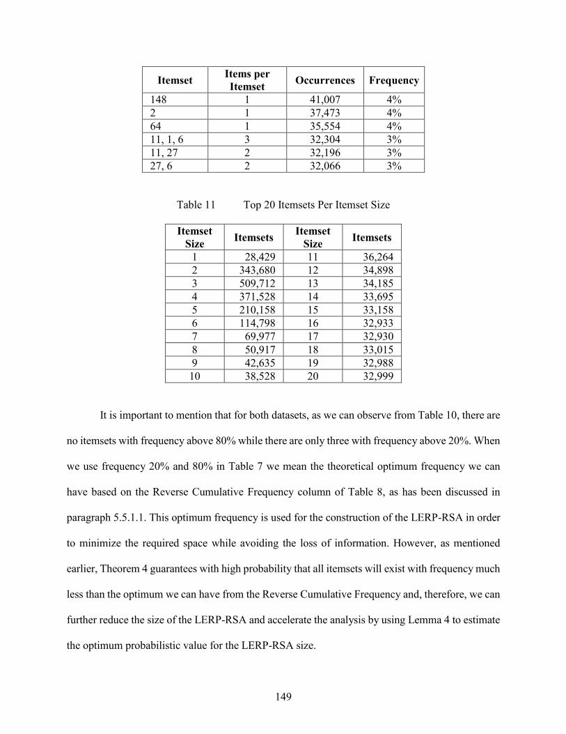
149

Itemset Items per

Itemset Occurrences Frequency

148 1 41,007 4%

2 1 37,473 4%

64 1 35,554 4%

11, 1, 6 3 32,304 3%

11, 27 2 32,196 3%

27, 6 2 32,066 3%

Table 11 Top 20 Itemsets Per Itemset Size

Itemset

Size Itemsets

Itemset

Size Itemsets

1 28,429 11 36,264

2 343,680 12 34,898

3 509,712 13 34,185

4 371,528 14 33,695

5 210,158 15 33,158

6 114,798 16 32,933

7 69,977 17 32,930

8 50,917 18 33,015

9 42,635 19 32,988

10 38,528 20 32,999

It is important to mention that for both datasets, as we can observe from Table 10, there are

no itemsets with frequency above 80% while there are only three with frequency above 20%. When

we use frequency 20% and 80% in Table 7 we mean the theoretical optimum frequency we can

have based on the Reverse Cumulative Frequency column of Table 8, as has been discussed in

paragraph 5.5.1.1. This optimum frequency is used for the construction of the LERP-RSA in order

to minimize the required space while avoiding the loss of information. However, as mentioned

earlier, Theorem 4 guarantees with high probability that all itemsets will exist with frequency much

less than the optimum we can have from the Reverse Cumulative Frequency and, therefore, we can

further reduce the size of the LERP-RSA and accelerate the analysis by using Lemma 4 to estimate

the optimum probabilistic value for the LERP-RSA size.

150

5.7 Data Stream Analysis

The LERP-RSA data structure and the ARPaD algorithm can be used for data streams

analysis. In the current paragraph, two general approaches will be introduced, the Sequential and

Dynamic Execution.

5.7.1 Sequential Execution

The Sequential Execution methodology for data stream analysis is divided into three phases

(Figure 25). First, the data structure has to be constructed and this process can be divided into three

steps. The first step is to determine the discretization method of our data, if we use real number

values and then determine the length of each subsequence that will be used for our data entries.

For example, in case of seismic waves analysis collected per second we may decide to analyze

strings per minute (60 data points) or 10 minutes (600 data points). Another prerequisite of the

methodology is to determine the Classification Level based on the alphabet used from the

discretization process. Another technique is the dynamic classification as presented in transactions

analysis paragraph. If dynamic classification is used, then a pre-statistical analysis has to be

executed on an substantial part of the inserted data points which will allow us to determine the

Classification Level for specific classes dynamically. For example, we can determine that when

10% of the subsequence has entered the system, then we check the size of the classes and, based

on the results, we change the Classification Level. If one or two classes are dominant in size, i.e.,

hold the majority of the data points, then we change the classification level of those classes and

create more but smaller classes. After defining the Classification Level, we have to determine the

size of each substring by calculating the LERP value using the Lemma 4.

151

Figure 25 Data Stream Analysis Sequential Execution

The second step of the first phase is the actual collection of the substrings of the LERP-

RSA data structure. When the first data point enters the system, it is stored temporarily and every

subsequent data point that enters the system is added to the string composed of pre-inserted data

points. When the length of the initial string reaches the size of the LERP value, then the string is

stored in the appropriate class and the first digit is removed. Therefore, we have saved a substring

of length equal to LERP in the system and we have e temporal string of length LERP-1. When the

next data point enters then a new string of length LERP is constructed, stored in the appropriate

152

class and the first digit is removed again. This process will repeat as many times as the length of

the subsequence. At the end of the first phase, this will lead to the creation of classes that hold in

total as many substrings as the length of the subsequence it has determined in the first step.

The third step is the sorting process of the LERP-RSA. This is the most time-consuming

part of the analysis. Each class of substrings has to be sorted, thus producing the lexicographically

sorted version of the LEPR-RSA in 𝑂(𝑛 log 𝑛) time. This phase can be executed in full parallel

mode since each class can be stored in different computers, achieving an extraordinary

performance and very short total sorting time.

The second phase of the methodology is the execution of the ARPaD algorithm on each

class with the parallel execution over each class simultaneously. The ARPaD algorithm is faster

than the sorting process, 𝑂(𝑛) on average, and it is the second most time-consuming step in our

methodology. Furthermore, usually the results have to be saved on disk in order to be analyzed

later which makes the algorithm execution slower. However, the overall time is insignificant as

we will observe in the experimental analysis section.

The third phase is meta-analyses processes. Having detected all repeated patterns, we can

run several predetermined scenarios on the results in order to mine valuable knowledge from them.

This process can be very fast since we search the results directly using pre-built models.

Furthermore, this process can also be executed in parallel using a different system while the

resources of the core computer systems are used again for the LERP-RSA creation and the ARPaD

execution of the next subsequence.

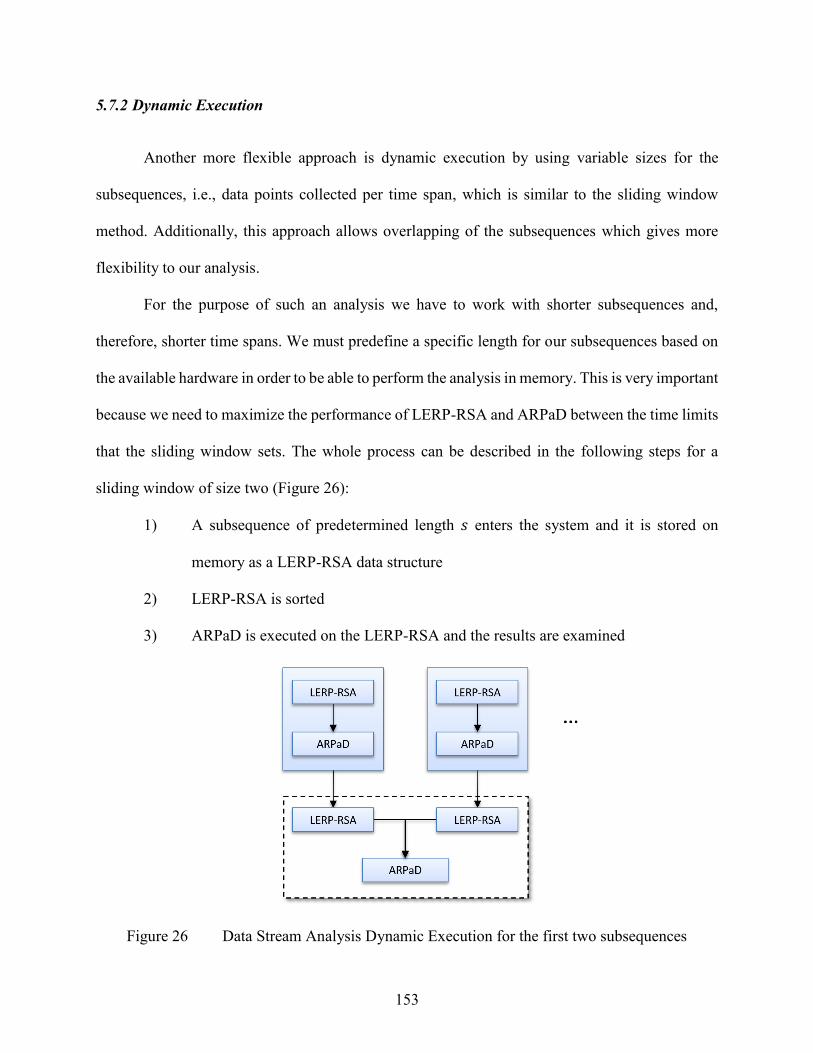
153

5.7.2 Dynamic Execution

Another more flexible approach is dynamic execution by using variable sizes for the

subsequences, i.e., data points collected per time span, which is similar to the sliding window

method. Additionally, this approach allows overlapping of the subsequences which gives more

flexibility to our analysis.

For the purpose of such an analysis we have to work with shorter subsequences and,

therefore, shorter time spans. We must predefine a specific length for our subsequences based on

the available hardware in order to be able to perform the analysis in memory. This is very important

because we need to maximize the performance of LERP-RSA and ARPaD between the time limits

that the sliding window sets. The whole process can be described in the following steps for a

sliding window of size two (Figure 26):

1) A subsequence of predetermined length 𝑠 enters the system and it is stored on

memory as a LERP-RSA data structure

2) LERP-RSA is sorted

3) ARPaD is executed on the LERP-RSA and the results are examined

Figure 26 Data Stream Analysis Dynamic Execution for the first two subsequences

154

Figure 27 Data Stream Analysis Dynamic Sliding Window Execution

This is the execution process for the first subsequence that enters the system. After the first

execution and having stored the LERP-RSA in memory, the full process can be described as

follows (Figure 27):

1) A new subsequence of predetermined length 𝑠 enters the system and it is stored on

memory as a new LERP-RSA data structure

2) The new LERP-RSA is sorted

3) ARPaD is executed on the new LERP-RSA and the results are examined

4) After step (2) the new LERP-RSA is merged with the old LERP-RSA

5) ARPaD is executed on the merged LERP-RSA

6) The merged LERP-RSA is disposed from memory together with the oldest existing

LERP-RSA.

It must be mentioned that steps (3), (1) and (2) for any new subsequence entrance are

executed in parallel with steps (4) and (5). Although it seems is impossible, such a parallelism is

very easy to be implemented due to the speed of the ARPaD and the merging algorithms.

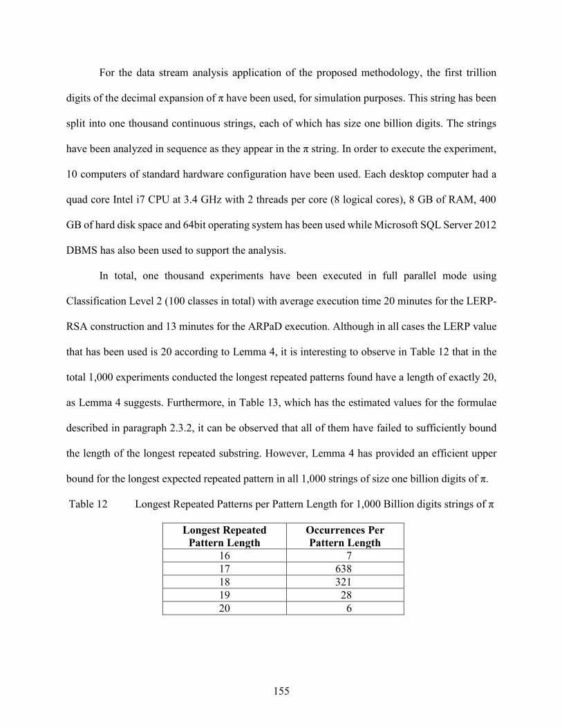
155

For the data stream analysis application of the proposed methodology, the first trillion

digits of the decimal expansion of π have been used, for simulation purposes. This string has been

split into one thousand continuous strings, each of which has size one billion digits. The strings

have been analyzed in sequence as they appear in the π string. In order to execute the experiment,

10 computers of standard hardware configuration have been used. Each desktop computer had a

quad core Intel i7 CPU at 3.4 GHz with 2 threads per core (8 logical cores), 8 GB of RAM, 400

GB of hard disk space and 64bit operating system has been used while Microsoft SQL Server 2012

DBMS has also been used to support the analysis.

In total, one thousand experiments have been executed in full parallel mode using

Classification Level 2 (100 classes in total) with average execution time 20 minutes for the LERP-

RSA construction and 13 minutes for the ARPaD execution. Although in all cases the LERP value

that has been used is 20 according to Lemma 4, it is interesting to observe in Table 12 that in the

total 1,000 experiments conducted the longest repeated patterns found have a length of exactly 20,

as Lemma 4 suggests. Furthermore, in Table 13, which has the estimated values for the formulae

described in paragraph 2.3.2, it can be observed that all of them have failed to sufficiently bound

the length of the longest repeated substring. However, Lemma 4 has provided an efficient upper

bound for the longest expected repeated pattern in all 1,000 strings of size one billion digits of π.

Table 12 Longest Repeated Patterns per Pattern Length for 1,000 Billion digits strings of π

Longest Repeated

Pattern Length

Occurrences Per

Pattern Length

16 7

17 638

18 321

19 28

20 6

156

Table 13 Upper Bounds Comparison for Largest Repeated Substring of 1,000 experiments

of 1 Billion digits strings from π

Formula Reference Bound

Value

2 log 𝑛

log (1𝜆)− [1 +

log(1 − 𝜆)

log 𝜆+0.5772

log 𝜆] +log 2

log 𝜆 [Kariln et al. 83] 17.23

𝑂 (log𝑁

log|𝛴|) [Manber and Mayers 90] 9

2 log𝑎 𝑛 + 𝑂(1) [Apostolico and

Szpankowski 92] 18

𝑂(2log 𝑛

log1

∑ 𝑝𝑖2

𝑖

) [Devroye et al. 92] 18

⌈⌈⌈⌈ 𝒍𝒐𝒈

𝒏𝟐

𝟐𝑷(𝑿)

𝒍𝒐𝒈𝒎

⌉⌉⌉⌉

LERP 20

Largest Repeated Substring’s Length Discovered

Experimentally - 20

5.8 Mathematics

The last application of the proposed methodology presented here, deals with Number

Theory and pure Mathematics. Champernowne Constant will be used to prove the concept of

randomness, while irrational numbers’ digits from their decimal and hexadecimal expansion will

be used to present the validity and efficiency of the methodology. Most of the material has been

published in [Xylogiannopoulos et al. 14a, 16b].

157

5.8.1 Randomness

Although it is known that Champernowne constant is not random as randomness is strictly

defined, due to the recursive construction of the constant, yet, the fact that it is proven to be normal

satisfies the prerequisites of Preposition 1. This is true since not only all alphabet letters are almost

equally distributed, but also every arrangement of letters up to a specific length relative to string

length exists with the appropriate frequency. Furthermore, the specific experiments show the

relation of the considerably long string and the reasonably long pattern. In these experiments, the

decimal digits of the most well-known mathematical constant for normal numbers have been used

as the strings for analysis. For the specific experiments the alphabet used is the decimal metric

system 𝛴 = {0, 1, 2, 3, 4, 5, 6, 7, 8, 9} with length 𝑚 = 10. The data string can be easily constructed

by a for-loop which each time adds the counter of the loop at the end of the already constructed

string of integers. [Xylogiannopoulos et al. 16b]

The Champernowne constant has been analyzed for different decimal digits length

[Xylogiannopoulos et al. 16b], trying to examine if there is a pattern followed in the results. More

specifically, four strings have been constructed for all integers from 1 up to 9,999 with string’s

length 𝑛 = 38,889, 1 to 99,999 with string’s length 𝑛 = 488,889, 1 to 999,999 with string’s length

𝑛 = 5,888,889 and 1 to 9,999,999 with string’s length 𝑛 = 68,888,889. In Table 14 it can be

observed how the numbers of repeated patterns per substring length are distributed while in Table

15 it can be observed that LERP values have efficiently upper bound the longest patterns found in

each experiment, something expected since Champernowne constant is a normal number and

satisfies Preposition 1.

From Table 16 with location, dispersion and shape parameters it can be observed that Mean

increases by a factor of one each time, while Standard Deviation remains constant at almost 0.7,

158

coefficient of Skewness remains approximately constant around -0.1, and coefficient of Kurtosis

fluctuates around 1.7. Knowing that Normal distribution 𝑁(0,1) has values of Standard Deviation

1, coefficient of Skewness 0 and coefficient of Kurtosis 0, the results in Table 16 are very close to

the parameters of Normal distribution. Therefore, from the experimental results we may conjecture

that when the string is random, the length of the repeated patterns follow the normal distribution.

Moreover, the length is very small compared to the length of the string and does not change

dramatically as the size of the string grows. On the contrary, the distributions of the patterns’

lengths, by following the Normal distribution, are distributed in a very small width and they are

upper bounded as Theorem 4 proposes. All the experimental results verify the proposed theory.

However, as we can see in Table 17 which has the estimated values for the last experiment

(string length 68,888,889) for the formulae described in paragraph 2.3.2, it can be observed that all

of them have failed to sufficiently bound the length of the longest repeated substring, although

2 log𝑎 𝑛 + 𝑂(1) and 𝑂 (2log𝑛

log1

∑ 𝑝𝑖2

𝑖

) (which directly derives from the previous) forms the best

approximation among the formulae and seems to give values very close to the actual, yet, below. It

has to be mentioned that the specific formula describes the “average height” [Apostolico and

Szpankowski 92] of the suffix tree and that is probably why it cannot sufficiently bound the actual

value of the specific string unless we assign a rather large value to the constant compared to the rest

of the formula calculation. However, Lemma 4 has provided an efficient upper bound for the longest

expected repeated pattern in Champernowne sequence, something that has also been observed in

paragraph 5.7.

159

Table 14 Occurrences per Pattern Length for Champerowne Constant

Occurrences

String Length(n) → 38,889 488,889 5,888,889 68,888,889

Substring Length ↓

1 10 10 10 10

2 100 100 100 100

3 1,000 1,000 1,000 1,000

4 9,065 10,000 10,000 10,000

5 9,074 91,094 100,000 100,000

6 7,406 98,480 911,462 1,000,000

7 929 89,116 1,000,334 9,117,331

8 15 73,862 975,578 10,081,794

9 9,044 885,982 9,930,962

10 30 738,247 9,716,432

11 15 90,212 8,849,087

12 45 7,380,159

13 30 900,127

14 15 82

15 45

16 30

17 15

Total Occurrences 27,559 372,751 4,713,015 57,087,174

Table 15 Theoretical and Actual LERP for Champernowne Constant

String

Length (n) 𝑷(𝑿)

Alphabet

(m)

Theoretical

LERP

Actual Longest

Repeated

Pattern

38,889 0.01 10 11 8

488,889 0.01 10 14 11

5,888,889 0.01 10 16 14

68,888,889 0.01 10 18 17

160

Table 16 Location, Dispersion and Shape Parameters for Champernowne Constant

Experiments

String

Length (n) Q1 Q2 Q3 Mean

Std.

Deviation. Skewness Kurtosis

38,889 4 5 6 4.92 0.96 0.02 -0.46

488,889 5 6 7 6.40 1.21 0.06 -0.79

5,888,889 7 8 9 7.89 1.48 0.06 -0.94

68,888,889 8 9 11 9.37 1.75 0.06 -1.01

Table 17 Upper Bounds Comparison for Largest Repeated Substring of Champernowne

Constant of length 68,888,889

Formula Reference Bound

Value

2 log 𝑛

log (1𝜆)− [1 +

log(1 − 𝜆)

log 𝜆+0.5772

log 𝜆] +log 2

log 𝜆 [Kariln et al. 83] 14.85

𝑂 (log𝑁

log|𝛴|) [Manber and Mayers 90] 7.84

2 log𝑎 𝑛 + 𝑂(1) [Apostolico and

Szpankowski 92] 15.68

𝑂(2log 𝑛

log1

∑ 𝑝𝑖2

𝑖

) [Devroye et al. 92] 15.68

⌈⌈⌈⌈ 𝒍𝒐𝒈

𝒏𝟐

𝟐𝑷(𝑿)

𝒍𝒐𝒈𝒎

⌉⌉⌉⌉

LERP 18

Largest Repeated Substring’s Length Discovered

Experimentally - 17

5.8.2 LERP-RSA and ARPaD Efficiency

In order to prove the validity and efficiency of the LERP-RSA data structure and ARPaD

algorithm a series of experiments on large strings of irrational numbers have been conducted for

161

the first time in [Xylogiannopoulos et al. 14a]. The specific methodology has been used for the

first time to prove that the decimal expansions of the irrational numbers π, e, φ and √2 are Normal

Numbers for the first 100 million digits. Indeed, such an experiment has never been conducted

because there was no algorithm which could detect all repeated patterns that exist in a string

[Xylogiannopoulos et al. 14a]. However, LERP-RSA and ARPaD made this feasible for the first

time in the history of Mathematics since 1909 when the problem was first stated by Émile Borel

[Borel 09].

Although this kind of experiment has never been executed, nevertheless, the specific

lengths of strings (100 million) do exist in literature for pattern detection purposes but only for

single pattern detection rather than all repeated patterns detection. In order to show that LERP-

RSA has unique attributes and flexibility that allows the analysis of very large strings compared

to any other data structure which is used for such purposes in literature, another experiment has

been conducted in [Xylogiannopoulos et al. 16b]. In the specific experiment, the first 64 GB digits

of the hexadecimal expansion of π, constructed with y-cruncher software [Yee 13], have been

analyzed using LERP-RSA and ARPaD. The importance of the size of the string can be

demonstrated if it is compared to the DNA string which is only 3.4 billion characters long (4 digits

alphabet), yet, it is considered one of the most difficult tasks in data mining literature and as has

been discussed in paragraph 5.3 even the analysis of a single chromosome can be extremely

difficult or unfeasible. The string analyzed in [Xylogiannopoulos et al. 16b] is 20 times larger than

DNA and took a significantly short time to be analyzed. In order to execute the experiment 16

computers of standard hardware configuration have been used. Each desktop computer had a quad

core Intel i5 CPU at 2.8 GHz with 2 threads per core (8 logical cores), 8 GB of RAM, 400 GB of

162

hard disk space and 64bit operating system has been used while Microsoft SQL Server 2012

DBMS has also been used to support the analysis.

The experiment was conducted in full-parallel mode using Classification Level 2 LERP-

RSA in Indeterminacy State (256 classes) and 16 computers analyzing 16 classes each with 16

threads on each computer. Table 18 reports the number of repeated patterns detected per pattern

length, including the cumulative number of detected patterns. As can be observed, not only the

size of the string for the experiment is enormous (almost 68 billion digits) but also the detected

patterns which are almost 25 billion. Given the fact that the total execution time was approximately

51 days, it means that on average ARPaD algorithm using the Full-Parallel/Classification

methodology detected a pattern every 0.00018 seconds. This average seek time is extremely fast

compared to any algorithm that can be used to detect a single pattern. However, direct comparison

to other algorithms cannot made since to the best of my knowledge ARPaD is the only algorithm

of this kind that exists in literature. The use of classification, parallelism and distributed computing

allows compressing the analysis execution time to an extreme level, in relation to the string that

has to be analyzed.

Table 18 Patterns and Cumulative Occurrences per Pattern Length for 68GB string of π

Pattern

Length

Patterns Per

Pattern Length

Cumulative

Occurrences

1 16 16

2 256 272

3 4,096 4,368

4 65,536 69,904

5 1,048,576 1,118,480

6 16,777,216 17,895,696

7 268,435,456 286,331,152

8 4,294,959,216 4,581,290,368

163

Pattern

Length

Patterns Per

Pattern Length

Cumulative

Occurrences

9 18,158,567,797 22,739,858,165

10 2,060,035,325 24,799,893,490

11 133,876,005 24,933,769,495

12 8,385,840 24,942,155,335

13 523,171 24,942,678,506

14 32,507 24,942,711,013

15 1,994 24,942,713,007

16 126 24,942,713,133

17 4 24,942,713,137

As a proof of the experiments’ execution, Table 19 reports the substrings (patterns) found

with the least occurrences per length and Table 20 the substrings found with the most occurrences

per length. In these two tables substrings with length up to 5, 6 and 7 digits have been presented

since for longer lengths a vast number of substrings occur and it is impossible to be presented here

(with length 8, millions of substrings occur each one from 2 up to 46). Moreover, Table 21 presents

the substrings found for the longest repeated patterns, i.e., substrings with length 17 for length 64GB

(4 in total). It is very important to mention that if any kind of brute force algorithm or technique is

applied to detect these 4 substrings of the last experiments (assuming that we have the hardware

needed to construct the appropriate data structure for such an algorithm) we have to check 1615

different arrangements or 295,147,905,179,352,825,856 different substrings (approximately 295

thousand trillion). Even if we have a data structure and an algorithm that can check a substring

every nanosecond (10−9 which actually we do not have with the currently existing hardware) this

means that we need approximately 295,147,905,179 seconds to check every possible substring or

3,416,063 days, assuming of course that the data structure can be constructed using any other

method. This case stands just for substrings of the specific length 17 and not for every smaller

164

length, since in order to repeat this brute force process for every length between 1 and 17, hundreds

of millions of years will be needed. The outcome of these experiments proves the novelty and

superiority of the methodology, the LERP-RSA data structure which allows classification and

parallelism and the ARPaD algorithm which can take advantage of the unique characteristics of

LERP-RSA data structure.

Table 19 Least Patterns per Pattern Length for 68GB string of π

Pattern

Length Pattern Occurrences

1 2 4,294,867,773

2 70 268,395,157

3 A8A 16,759,617

4 8E31 1,044,270

5 BF640 64,305

6 904F8E 3,761

7 ACAD9B6 164

Table 20 Most Patterns per Pattern Length for 68GB string of π

Pattern

Length Pattern Occurrences

1 B 4,295,046,897

2 A1 268,485,359

3 A34 16,792,240

4 389F 1,052,848

5 95C7C 66,761

6 8DE185,

E5EC53 4,442

7 794AE4C 355

Table 21 Longest Repeated Pattern for 68GB string of π

Pattern

272B6BCF43B705682

80DD746990ECDEDDF

165

Pattern

BB2D9D87805C044A3

C25D98ED123313833

5.8.3 Irrational Numbers and Big Data

The last experiment presented in my thesis concerns big data mining. Again, the decimal

digits from π will be used because:

1) It is the only irrational number (or notion in general) for which up to 13.2 trillion

digits are known, making it the biggest sequence ever constructed, directly or

indirectly, in science [Yee, 13, CALICO 15],

2) The specific sequence is deterministic and, therefore, anyone can use exactly the

same to conduct any kind of experiments for comparison purposes and

3) According to [Bailey et al. 12, Xylogiannopoulos et al. 14a, 16b] it has been shown,

theoretically and experimentally, that π is a Normal Number with very high

probability.

In this last experiment, the first 1 Trillion digits of the decimal expansion of π, obtained

from [CALICO 15], will be analyzed and all repeated patterns will be detected using advanced

ARPaD. The specific string is approximately 15 times larger than the experiment presented in

paragraph 5.8.2 and 330 times larger than the human DNA genome. Ten desktop computers have

been used with an Intel i7 CPU at 3.4 GHz with 2 threads per core (8 logical cores), 8 GB of RAM,

400 GB of hard disk space and 64bit operating system has been used. In this experiment, it was

impossible to use Microsoft SQL Server 2012 DBMS due to insufficient resources for the needs

of the experiment. Due to this limitation, text files have been used in a Classification Level 3 and

Classification Level 5 combination to support the analysis. The two different types of

166

Classification Levels are absolutely necessary in order to overpass limitations caused by operating

systems, file systems and programming languages.

As a proof of the experiments’ execution, Table 22 reports the number of repeated patterns

detected per pattern length, including the cumulative number of detected patterns while the two

longest repeated patterns found can be observed in Table 23. As can be observed, the size of the

one Trillion digits string for the experiment is enormous and has been reached for the first time in

any kind of data mining analysis to the best of my knowledge. Furthermore, the detected patterns

accumulate to the incredible size of more than 427 billion patterns. On average the execution time

per pattern was 3.2 microseconds (0.0000032 sec) or 312,500 patterns per second approximately.

The above-mentioned execution time covers on average both the LERP-RSA construction and the

ARPaD execution.

It should be mentioned that the LERP used for the specific experiment is 26, which means

that the size of the data structure that had to be constructed was approximately 40TB in total. This

amount of disk space was not available and, therefore, the execution of the experiment was made

feasible only by using the full combination of all attributes of LERP-RSA, i.e., Semi-Parallel

Classification and Execution, Network Distribution, Compression and Indeterminacy.

Furthermore, it is also important to mention that although 40TB may not seem like big data, yet,

the 1 Trillion digits of π is a single piece of information and has to be analyzed as it is, making the

task an important achievement for the available resources, which can be definitely characterized

as Big Data Analytics.

167

Table 22 Patterns and Cumulative Occurrences per Pattern Length for 1 Trillion decimal

digits string of π

Pattern

Length

Patterns Per Pattern

Length

Cumulative

Occurrences

1 10 10

2 100 110

3 1,000 1,110

4 10,000 11,110

5 100,000 111,110

6 1,000,000 1,111,110

7 10,000,000 11,111,110

8 100,000,000 111,111,110

9 1,000,000,000 1,111,111,110

10 10,000,000,000 11,111,111,110

11 99,950,065,779 111,061,176,889

12 264,241,335,164 375,302,512,053

13 46,788,356,352 422,090,868,405

14 4,966,774,344 427,057,642,749

15 499,655,710 427,557,298,459

16 49,987,809 427,607,286,268

17 4,995,035 427,612,281,303

18 498,835 427,612,780,138

19 49,518 427,612,829,656

20 4,883 427,612,834,539

21 459 427,612,834,998

22 40 427,612,835,038

23 2 427,612,835,040

Table 23 Longest Repeated Patterns in the first 1 Trillion decimal digits of π

Pattern Positions

64722721994615606186022 2,806,926,755

486,503,740,532

85018258601373450524625 284,298,924,311

486,740,822,467

168

5.9 Image Analysis

An image analysis problem can be transformed to a transactions analysis and, therefore,

every two-dimension (or more) image can be decomposed to a single dimension, multivariate,

string problem as we have observed in previous paragraphs with transactions analysis, clickstreams

analysis, network analysis etc. The ability to perform such an analysis can be very useful in many

cases such as compression (as described in the next paragraph) and similarities checking between

images. In particular, a similarity check can be applied in medical image analysis, forensic,

fingerprint recognition and matching, optical character recognition etc.

An example of image analysis can be described with the images of “Figure 28” which

represents a clear image of the Greek letter Γ (Figure 28.a) and an unclear image of the letter Γ

(Figure 28.b). As discussed above, every two-dimensional image can be decomposed to a single

dimension string and transformed to a transactions analysis problem. Every image can be

considered as a two-dimensional array holding the color value (bit) of the image in each cell of the

array. Therefore, we can consider every row as a transaction composed of every possible color bit

value we can have. In the example of the Γ letter image, if we assume that we use only the two

colors, black and white, (2bit) then the first row can be represented as “01111000”. Since in most

of the cases images use 32bit color depth (as in the current example), then the first row of the

image can be expressed as “ffffffffff000000ff000000ff000000ff000000ffffffffffffffffffffffff”, in

which every block of eight characters represents a 32bit color value and more specifically “ffffffff”

for white and “ff000000” for a grey variation. The second representation is exactly the same as in

the case of a transaction analysis where a numerical alphabet has been used to represent items. In

this case, however, items are hexadecimal color values ranging from “00000000” for black up to

“ffffffff” for white.

169

Figure 28 Clear and unclear images of Greek letter Γ

In the specific example, we can observe that the horizontal part of letter Γ, with length four,

occurs in the first image from position (0,1) to position (0,4) and in the second image from position

(2,3) to position (2,6). The vertical part occurs in the first image from position (0,1) to position

(5,1) and in the second image from position (2,3) to position (7,3). As discussed earlier, we should

apply the same methodology as we did with transactions and clickstreams analysis. Therefore, we

decompose each image to their rows and create the corresponding LERP-RSA. Then we mix all

LERP-RSA data structures and execute the ARPaD algorithm. After ARPaD execution we receive

several patterns as results (due to noise presence in second image) but the most important patterns

are the following:

1) “ff000000ff000000ff000000ff000000” at position (0,1) for the first image and

position (2,3) for the second.

2) “ff000000ffffffff” at positions {(1,1), (2,1), (3,1), (4,1), (5,1)} for the first image

and positions {(3,3), (4,3), (5,3), (6,3), (7,3)} for the second image.

We can observe from these results that letter Γ also exists in the second image shifted by two pixels

to the right and two pixels to the bottom.

170

This is just one example of an application of image analysis that LERP-RSA and ARPaD

can have. The specific methodology can be used for many purposes in order to detect, e.g.,

similarities for medical purposes, compression, fingerprints analysis etc.

5.10 Compression

The ARPaD algorithm can be used for compression purposes of any type. The ability to

know all repeated patterns and their positions allows us to store patterns only once with their

corresponding positions. Indexes of positions, represented as integers, consume much less space

than actual strings and, therefore, we can perform a significant compression level which can reach

approximately 60%. More detailed, we can have two cases of strings with regard to the pattern

distribution. Either a string is random and, therefore, the pattern distribution follows the pattern

distribution we have observed in the case of π or a string is not random and, therefore, we can

assume that pattern distribution could be similar to, e.g., DNA strings.

In the first case, the following approach can be used. As we can observe from the results

of the experiment of the first trillion digits from π in Table 22, almost every pattern with length up

to 11 digits exists twice. This guarantees that if we use the particular length patterns, the whole

string will be fully covered. Therefore, we can reconstruct the string if we save the positions of

these patterns instead of the actual patterns. One clever way to do this is to store the positions as

an array in which each row refers to the corresponding pattern, e.g., the first position represents

pattern “00000000000”, the second “00000000001” etc. Doing this allows us to store an 8 byte

integer instead of an 11 byte string and perform approximately 27% compression. However, we

can further improve compression by storing positions as a two-dimensional array in which every

row refers to the corresponding pattern (as above) and every column corresponds to a block of

integers of 4 bytes. Although each column holds integer values from 0 up to 4,294,967,295 (4 byte

171

or 32bit integer), every column, except the first, holds the relative position according to the column

index. For example, the second column holds integers from 4,294,967,296 up to 8,589,934,691 (as

4 byte relative positions) and, therefore, for a pattern which appears, e.g., in position 4,294,967,296

in the string, instead of this value we store value 0 in the second column. Using the methodology,

we can have 4 byte integers stored instead of 11 byte patterns and, therefore, perform a

compression of approximately 60%.

In the second case when a string is random, e.g., DNA or any simple text, the appearance

of every pattern up to a significant length cannot be guaranteed. However, we have several

extremely long patterns which can have a length of several tens or hundreds of characters and can

save significant space while they balance the absence of patterns of specific length as in the first

case. Again, the same methodology as in the first case can be used to achieve exceptionally good

results by using a hash function to convert each pattern to a corresponding integer value, which

will be used in an array. Another approach, avoiding hash function, is to store both patterns and

their positions which reduces the ratio of compression but it can be faster.

In both cases the reconstruction of the original string can be easily executed from the

patterns (actual or encoded based on array indexes or hash functions) and their corresponding

positions. Furthermore, it is important to mention that this methodology can be applied to single

strings but also to multiple strings representing, e.g., images.

5.11 Text Mining

Text mining is a direct application of the LERP-RSA data structure and the SPaD, MPaD,

MvdPaD and ARPaD algorithms, as presented in previous paragraphs of the current chapter. Every

example from previous paragraphs and analyses performed are indirect applications of text mining

in either single text sequences such as in π and DNA strings or multivariate text sequences such as

172

transactions, clickstreams analysis, image analysis etc. In the first case, we may have single strings

which can be considered single line texts, e.g., text from a book or manuscript. In the second case,

we may have multiple strings representing several books, manuscripts, emails etc.

As presented in many examples in previous paragraphs, all algorithms presented in this

thesis can achieve extraordinary results very fast and with limit resources. In the case of text

mining they have the additional advantage to detect patterns not only based on standard alphabets

coming from natural languages but also to use artificial alphabets. These alphabets may have been

constructed to represent items (transactions and clickstreams analysis) but also more general and

abstract notions such as color values in case of an image analysis. This allows to transform many

problems of pattern detection to text mining despite the fact that initially may seem completely

irrelevant.

The detection of all repeated patterns can be crucial for text mining purposes in many cases

and can easily be performed using the ARPaD algorithm with the LERP-RSA data structure. For

example, the detection of repeated patterns can be used for text similarities and plagiarism

detection in publications, student assignments etc. since ARPaD can detect repeated pattern in one

or more distinct texts. Another application can be for forensic reasons such as analysis of standard

or encrypted messages submitted via email, sms or other formats from any electronic device. The

potential of such analyses using the ARPaD algorithm and the LERP-RSA data structure is

limitless.

173

Chapter 6 Conclusions and Future Research

6.1 Synopsis

Concluding my thesis, the research work presented here can be summarized as follows:

1) The mathematical foundation has been built which allows the efficient calculation

of the Longest Expected Repeated Pattern that can exist in a string,

2) Based on the above, the novel data structures RSA and LERP-RSA, have been

introduced which although they use actual suffix strings, the space complexity has

been limited to log-linear, in the worst case. However, on average it has been

proven that it is linear, if the Classification property is used, and proved to be very

powerful and flexible,

3) Even when LERP as calculated does not manage to provide an accurate upper

bound and, therefore, information is lost, MLERP can be used to retain information,

4) The unique ARPaD algorithm has been introduced which is the only algorithm

existing in literature, to the best of my knowledge, that can allow the detection of

all repeated patterns in a string,

5) SPaD algorithm has been introduced which can allow the detection of single

patterns, in constant time complexity, using LERP-RSA,

6) MPaD algorithm has been introduced which can allow the detection of multiple

patterns in constant time complexity, using LERP-RSA,

7) It has been presented how all algorithms can be used for pattern detection using

wildcards,

174

8) The MvdPaD method has been introduced that allows the pattern detection in

multivariate systems or multidimensional variables and

9) Several applications of the above proposed data structures and algorithms have

been presented giving solutions to real-life scientific and commercial problems.

The proposed research work in the current thesis is a complete framework that allows any

kind of pattern detection in any kind of discrete sequences using limited hardware resources, and,

therefore, bypassing all known limitations Computer Science and more specifically Data Science

has faced so far in the specific field.

6.2 Future Research

Although the proposed work is a complete framework that covers all aspects in pattern

detection, yet, there is always space for further improvements. This is something which, hopefully,

I will have the opportunity to do by continuing my research work or other computer scientists may

want to perform based on the work presented here. Furthermore, despite the several applications

in many diverse problems presented in the fifth chapter, it is a strong belief of mine that the

proposed methodologies can be used to provide solution to many more problems. Again, this is a

process which will continue in the future in cooperation with either scientists from other scientific

fields or industry to provide scientific and commercial solutions.

175

Bibliography

[Agrawal and Srikant 95] Agrawal, R. and Srikant, R., “Mining sequential patterns,” in

Proceedings of 11th International Conference on Data Engineering (ICDE’95), P. S. Yu

and A. S. P. Chen, Eds. IEEE Computer Society Press, Taipei, Taiwan, (1995), pp. 3–14

[Akerkar and Akerkar 07] Akerkar, R. and Akerkar, R., “Discrete Mathematics,” Pearson

India, (2007)

[Al–Rawi et al. 03] Al–Rawi, A., Lansari, A. and Bouslama, F., “A New Non–Recursive

Algorithm for Binary Search Tree Traversal,” in Proceedings of IEEE Int’l Conf.

Electronics, Circuits and Systems, 2(2003), pp. 770–773

[Apostolico and Preparata 83] Apostolico, A. and Preparata, F. P., “Optimal Off–line

Detection of Repetitions in a String,” Theoretical Computer Science, 22(1983), pp. 297–

315

[Apostolico and Szpankowski 92] Apostolico, A. and Szpankowski, W., “Self–alignment in

Words and their Applications,” Journal of Algorithms, 13:3(1992), pp. 446–467

[Ayres et al. 02] Ayres, J., Flannick, J., Gehrke, J. and Yiu, T., “Sequential pattern mining using

a bitmap representation,” in Proceedings of the eighth ACM SIGKDD international

conference on Knowledge discovery and data mining, (2002), pp. 429–435

[Bailey et al. 97] Bailey, D. H., Borwein, P. B. and Plouffe, S., “On the rapid computation

of various polylogarithmic constants,” Mathematics of Computation, 66:218(1997), pp.

903–913

[Bailey and Crandall 01] Bailey, D. H. and Crandall, R. E. “On the Random Character of

Fundamental Constant Expansions,” Experimental Mathematics, 10:2(2001), pp. 175–190

176

[Bailey and Crandall 02] Bailey, D. H. and Crandall, R. E. "Random Generators and Normal

Numbers," Experimental Mathematics, 11:4(2002), pp. 527–546

[Bailey et al. 12] Bailey, D. H., Borwein, J. M., Calude, C. S., Dinneen, M. J., Dumitrescu,

M. and Yee A., “An Empirical Approach to the Normality of π,” Experimental

Mathematics, 21:4(2012), pp. 375–384

[Barsky et al. 11] Barsky, M., Stege, U. and Thomo A., “Suffix Trees for Inputs Larger than

Main Memory,” Information Systems, 36:3(2011), pp. 644–654

[Becher 12] Becher, V., “Turing’s Normal Numbers: Towards Randomness” in Cooper, B.

S., Dawar, A. and Löwe B. (Eds.) “How the World Computes: Lecture Notes in Computer

Science,” Springer 7318(2012), pp. 35–45

[Bodie et al. 10] Bodie, Z., Kane, A., and Marcus, A. J., “Investments and Portfolio

Management,” 9th Revised Global Edition, McGraw–Hill Europe, (2010)

[Borel 09] Borel, E., “Les Probabilités Dénombrables et Leurs Applications Arithmétiques,”

Rend. Circ. Mat. Palermo, 27(1909), pp. 247–271

[CAIDA 08] CAIDA, “The UCSD CAIDA DDoS attack on August 4, 2007 (20:50:08 UTC to

21:56:16 UTC),” (2008), Available: http://www.caida.org/data/passive/ddos–

20070804_dataset.xml

[CALICO 15] CALICO, “PI-World site,” Available: http://piworld.calico.jp/index.html

[Calude 94] Calude, C., “Borel Normality and Algorithmic Randomness” in Rozenberg, G.

and Salomaa, A. (eds.). “Development in Language Theory,” World Scientific, (1994), pp.

113–129

[Calude 95] Calude, C., “What is a Random String?” Journal of Universal Science 1:1(1995),

pp. 48–66

177

[Cassels 59] Cassels, J. W. S., “On a problem of Steinhaus about normal numbers,”

Colloquium Mathematicum, 7:1(1959), pp. 95–101

[Chaitin 88] Chaitin, G. J., “Randomness in Arithmetic,” Scientific American, 259:1(1988),

pp. 80–85

[Champernowne 33] Champernowne, D. G., “The Construction of Decimals Normal in the

Scale of Ten,” Journal of the London Mathematical Society, 8(1933), pp. 254–260

[Chanda et al. 15] Chanda, A. K, Saha, S., Nishi, M. A., Samiullah, Md. And Ahmed C. F.,

“An efficient approach to mine flexible periodic patterns in time series databases,”

Engineering Applications of Artificial Intelligence, 44:C(2015), pp. 46–63

[Cheung et al. 05] Cheung, C.–F., Yu, J.X. and Lu, H., “Constructing Suffix Tree for

Gigabyte Sequences with Megabyte Memory,” IEEE Transactions on Knowledge and Data

Engineering, 17:1(2005), pp. 90–105

[Church 40] Church, A., “On the Concept of a Random Sequence,” Bulletin of the American

Mathematical Society, 46:2(1940), pp. 130–135

[Copeland and Erdös 46] Copeland, A. H. and Erdös, P., “Note on Normal Numbers,” Bulletin

of the American Mathematical Society, 52:10(1946), pp. 857–860

[Crauser and Ferragina 02] Crauser, A. and Ferragina, P., “A Theoritical and Experimental

Study on the Construction of Suffix Arrays in External Memory,” Algorithmica,

32:1(2002), pp. 1–35

[Dasgupta 11] Dasgupta, A., “Mathematical Foundations of Randomness,” in Gabbay, D. M.,

Thagard, P. and Woods, J., (Gen. Eds.), “Philosophy of Statistics” North Holland (2011),

Saint Louis, MO, USA, pp. 641–710

178

[Davenport and Erdös 52] Davenport, H. and Erdös, P., “Note on Normal Decimals,” Canadian

Journal of Mathematics, 4(1952), pp. 58–63

[De Koninck 15] De Koninck, J.–M., “The Mysterious World of Normal Numbers,” in

Beierle, C., and Dekhtyar, A., (Eds.), “9th International Conference, SUM 2015, Québec

City, QC, Canada, September 16–18, 2015. Proceedings,” (2015), pp.3–18, doi:

10.1007/978–3–319–23540–0_1

[Dementiev et al. 08] Dementiev, R., Karkkainen, J., Mehnert, J. and Sanders, P., “Better

External Memory Suffix Array Construction,” Journal of Experimental Algorithmics,

12(3.4)(2008), pages 24, unpaginated, doi: 10.1145/1227161.1402296

[Devroye et al. 92] Devroye, L., Szpankowski, W. and Rais, B., “A Note on the Height of

Suffix Trees,” SIAM Journal on Computing, 21:1(1992), pp. 48–53

[Elfeky et al. 05a] Elfeky, M. G., Aref, W. G. and Elmagarmid, A. K., “Periodicity Detection

in Time Series Databases,” IEEE Transactions of Knowledge and Data Engineering,

17:7(2005), pp. 875–887

[Elfeky et al. 05b] Elfeky, M. G., Aref, W. G. and Elmagarmid, A. K., “WARP: Time

Warping for Periodicity Detection,” in Proceedings of the Fifth IEEE International

Conference on Data Mining, (2005), pages 24, unpaginated, doi: 10.1109/ICDM.2005.152

[FIMI 04] Frequent Itemset Mining Dataset Repository, (2005), Available:

http://fimi.ua.ac.be/data/

[Franek et al. 03] Franek, F., Smyth, W. F. and Tang, Y., “Computing All Repeats Using

Suffix Arrays,” Journal of Automata, Languages and Combinatorics, 8:4(2003), pp. 579–

591

179

[Garofalakis et al. 99] Garofalakis, M. N., Rastogi, R. and Shim, K., “SPIRIT: Sequential Pattern

Mining with Regular Expression Constraints,” in Proceedings of the 25th International

Conference on Very Large Data Bases, 99(1999), pp. 223–234

[Gog et al. 13] Gog, S., Moffat, A., Culpepper, S., Turpin, A. and Wirth, A., “Large–Scale

Pattern Search Using Reduced–Space On–Disk Suffix Arrays,” arXiv:1303.6481v1,

(2013), pp. 1–14

[Gusfield 97] Gusfield D., “Algorithms on Strings, Trees, and Sequences,” Cambridge Univ.

Press, (1997)

[Han et al. 99] Han, J., Dong, G. and Yin, Y., “Efficient Mining of Partial Periodic Patterns in

Time Series Database,” in Proceedings of the 15th IEEE International Conference on Data

Engineering, (1999), pp. 106–115

[Hardy and Wright 60] Hardy, G. H. and Wright, E. M., “An Introduction to the Theory of

Numbers,” 4th Edition, Oxford University Press, (1960)

[Huang and Chang 05] Huang, K.–Y. and Chang, C.–H., “SMCA: A General Model for

Mining Asynchronous Periodic Patterns in Temporal Databases,” IEEE Transactions on

Knowledge and Data Engineering, 17:6(2005), pp. 774–785

[Hull 12] Hull, J. C., “Options, Futures, and Other Derivatives,” 8th Global Edition, Pearson

Education Limited, (2012)

[Karkkainen et al. 06] Karkkainen, J., Sanders, P. and Burkhardt, S., “Linear Work Suffix Array

Construction,” Journal of the Association for Computing Machinery, 53:6(2006), pp. 918–

936

[Khoshnevisan 06] Khoshnevisan, D., “Normal Numbers are Normal,” Clay Mathematics

Institute Annual Report 2006, 15(2006), pp. 27–31

180

[Kim et al. 03] Kim, D.K., Sim, J.S., Park, H. and Park, K., “Linear–Time Construction of

Suffix Arrays (Extended Abstract),” in Baeza–Yates, R., Chávez, E. and Crochemore, M.

(Eds) Combinatorial Pattern Matching, (2003), pp. 186–199

[Ko and Aluru 03] Ko, P. and Aluru, S., “Space Efficient Linear Time Construction of Suffix

Arrays,” in Proceedings of the 14th Annual Conference on Combinatorial Pattern Matching,

(2003), pp. 200–210

[Long 57] Long, C. T., “Note on Normal Numbers,” Pacific Journal of Mathematics, 7:2(1957),

pp. 1163–1165

[Mabroukeh and Ezeife 10] Mabroukeh, N. R. and Ezeife, C. I., “A taxonomy of sequential

pattern mining algorithms,” Journal of ACM Computing Surveys, 43:1[3](2010), pages 41,

unpaginated, doi: 10.1145/1824795.1824798

[Manber and Myers 90] Manber, U. and Myers, G., “Suffix Arrays: A New Method for On–

Line String Searches,” in Proceedings of the First Annual ACM–SIAM Symposium on

Discrete Algorithms, (1990), pp. 319–327

[Masseglia et al. 98] Masseglia, F., Cathala, F. and Poncelet, P., “The psp approach for mining

sequential patterns,” in Principles of Data Mining and Knowledge Discovery, (1998), pp.

176–184

[McCreight 76] McCreight, E. M., “A Space-Economical Suffix Tree Construction Algorithm,”

Journal of the Association for Computing Machinery, 23:2(1976), pp. 262–272

[Navarro and Baeza–Yates 99] Navarro, G. and Baeza–Yates, R., “A New Indexing Method

for Approximate String Matching,” in Proceedings of the 10th Annual Symposium

Combinatorial Pattern Matching, (1999), pp. 163–185

181

[Navarro and Baeza–Yates 00] Navarro, G. and Baeza–Yates, R., “A Hybrid Indexing Method

for Approximate String Matching,” Journal of Discrete Algorithms, 1:1(2000), pp. 205–

239

[Needleman and Wunsch 70] Needleman, S. B. and Wunsch, C. D., “A General Method

Applicable to the Search for Similarities in the Amino Acid Sequence of Two Proteins,”

Journal of Molecular Biology, 48:3(1970), pp. 443-453

[Nishi et al. 13] Nishi, M. A, Ahmed, C. F., Samiullah, Md. and Jeong, B.-S., “Effective periodic

pattern mining in time series databases,” Expert Systems with Applications, 40(2013), pp.

3015–3027

[Niven and Zuckerman 51] Niven, I. and Zuckerman, H., “On the Definition of Normal

Numbers,” Pacific Journal of Mathematics, 1:1(1951), pp. 103–109

[Orlandi and Venturini 11] Orlandi, A. and Venturini, R., “Space–efficient Substring

Occurrence Estimation,” in Proceedings of the 30th Principles of Database Systems PODS,

(2011), pp. 95–106

[Parker 09] Parker, M., “Pattern Search in a Single Genome,” Nuffield Science Bursary

Project, Oxford Centre for Gene Function, Oxford University Statistics, (2009), pp. 1–34

[Phoophakdee 07] Phoophakdee, B., “TRELLIS: Genome–scale Disk–based Suffix Tree

Indexing Algorithm,” PhD Thesis, Department of Computer Science, Rensselaer

Polytechnic Institute, Troy, (2007)

[Phoophakdee and Zaki 07] Phoophakdee, B. and Zaki, M., “Genome–scale Disk–based Suffix

Tree Indexing,” SIGMOD '07 in Proceedings of International Conference on Management

of Data, (2007), pp. 833–844

182

[Puglishi et al. 08] Puglishi, S. J., Smyth, W. F. and Yusufu, M., “Fast Optimal Algorithms

for Computing All the Repeats in a String,” in Proceedings of PSC 2008, (2008), pp. 161–

169

[Rasheed and Alhajj 08] Rasheed, F. and Alhajj, R., “Using Suffix Trees for Periodicity

Detection in Time Series Databases,” in Proceedings 4th International IEEE Conference

Intelligent Systems, 2(2008), pp. 11-8–11-13

[Rasheed et al. 10] Rasheed, F., Alshalfa, M. and Alhajj, R., “Efficient Periodicity Mining in

Time Series Databases Using Suffix Trees,” IEEE Transactions on Knowledge and Data

Engineering, 22:20(2010), pp. 1–16

[Schürmann and Stoye 05] Schürmann, K. B. and Stoye J., “An Incomplex Algorithm for Fast

Suffix Array Construction,” in Proceedings of the 7th Workshop on Algorithm Engineering

and Experiments and the 2nd Workshop on Analytic Algorithmics and Combinatorics

(ALENEX/ANALCO), (2005), pp. 77–85

[Sheng et al. 05] Sheng, C., Hsu, W. and Lee, M.–L., “Efficient Mining of Dense Periodic

Patterns in Time Series,” Technical Report, National University of Singapore, (2005), pp.

1–16

[Sheng et al. 06] Sheng, C., Hsu, W. and Lee, M.–L., “Mining Dense Periodic Patterns in

Time Series Data,” in Proceedings of 22nd International Conference on Data Engineering,

(2006), p. 115, doi: 10.1109/ICDE.2006.97

[Sierpiński 17] Sierpiński, W., “Démonstration élémentaire d'un théorème de M. Borel sur les

nombres absolument normaux et détermination effective d'un tel nombre,” Bulletin de la

Société Mathématique de France, 45(1917), pp. 127–132

183

[Sinha et al. 08] Sinha, R., Moffat, A., Puglisi, S. and Turpin, A., “Improving Suffix Array

Locality for Fast Pattern Matching on Disk,” in Proceedings of the International

Conference on Management of Data, (2008), pp. 661–672

[Smith and Waterman 81] Smith, T. F. and Waterman, M. S., “Identification of Common

Molecular Subsequences,” Journal of Molecular Biology, 147(1981), pp. 195-197

[Spivak 94] Spivak, M., “Calculus,” 3rd Edition, Publish or Perish, (1994)

[Tian et al. 05] Tian, Y., Tata, S., Hankins, R.A. and Patel, J.M., “Practical Methods for

Constructing Suffix Trees,” The International Journal on Very Large Data Bases,

14:3(2005), pp. 281–299

[UCSC 13] University of California Santa Cruz, “UCSC Genome Bioinformatics,” (2013),

Available: http://hgdownload.soe.ucsc.edu/goldenPath/hg38/chromosomes/

[Ukkonen 95] Ukkonen E., “Online Construction of Suffix Trees,” Algorithmica, 14:3(1995),

pp. 249–260

[Wagon 85] Wagon, S., “Is Pi Normal?” The Mathematical Intelligencer, 7:3(1985), pp. 65–

67

[Weiner 73] Weiner, P., “Linear Pattern Matching Algorithms,” in Proceedings of the 14th

Annual Symposium on Switching and Automata Theory (SWAT 1973), (1973), pp. 1–11

[Wong et al. 07] Wong, S.S., Sung, W.K. and Wong, L., “CPS–tree: A Compact Partitioned

Suffix Tree for Disk–based Indexing on Large Genome Sequences,” in Proceedings of

IEEE International Conference on Data Engineering, (2007), pp. 1350–1354

[Wu et al. 14] Wu, Y., Wang, L., Ren, J., Ding, W. and Wu, X., “Mining Sequential Patterns

with Periodic Wildcard Gaps,” Applied Intelligence, (2014), pp. 99–116

184

[Xylogiannopoulos et al. 12a] Xylogiannopoulos, K., Karampelas, P. and Alhajj, R.,

“Periodicity Data Mining in Time Series Using Suffix Arrays,” in Proceedings of the 6th

IEEE Conference Intelligent Systems, (2012), pp. 172–181, doi: 10.1109/IS.2012.6335132

[Xylogiannopoulos et al. 12b] Xylogiannopoulos, K., Karampelas, P. and Alhajj, R., “Pattern

Detection and Analysis in Financial Time Series Using Suffix Arrays,” in Doumpos, M.;

Zopounidis, C. and Pardalos, P. M. (Eds.), “Financial Decision Making Using

Computational Intelligence”, (2012), pp.129–157, doi: 10.1007/978-1-4614-3773-4_5

[Xylogiannopoulos et al. 12c] Xylogiannopoulos, K., Karampelas, P. and Alhajj, R.,

“Minimization of Suffix Array’s Storage Capacity for Periodicity Detection in Time

Series,” in Proceedings of the 24th IEEE International Conference on Tools with Artificial

Intelligence, 1(2012), pp. 307–313, doi: 10.1109/ICTAI.2012.49

[Xylogiannopoulos et al. 14a] Xylogiannopoulos, K., Karampelas, P. and Alhajj, R.,

“Experimental Analysis on the Normality of π, e, φ, sqrt(2) Using Advanced Data–Mining

Techniques,” Experimental Mathematics, 23:2(2014), pp. 105–128, doi:

10.1080/10586458.2013.878674

[Xylogiannopoulos et al. 14b] Xylogiannopoulos, K., Karampelas, P. and Alhajj, R.,

“Analyzing Very Large Time Series Using Suffix Arrays,” Applied Intelligence,

41:3(2014), pp. 941–955, doi: 10.1007/s10489–014–0553–x

[Xylogiannopoulos et al. 14c] Xylogiannopoulos, K., Karampelas, P. and Alhajj, R., “Early

DDoS Detection Based on Data Mining Techniques,” in Proceedings of the 8th

International Workshop in Information Security Theory and Practice, 8501(2014), pp.

190–199, doi: 10.1007/978-3-662-43826-8_15

185

[Xylogiannopoulos et al. 15a] Xylogiannopoulos, K. F., Karampelas, P. and Alhajj, R.,

“Discretization Method for the Detection of Local Extrema and Trends in Non-discrete

Time Series,” in Proceedings of the 17th International Conference on Enterprise

Information Systems, (2015), pp. 346–352, doi: 10.5220/0005401203460352

[Xylogiannopoulos et al. 15b] Xylogiannopoulos, K. F., Karampelas, P., Alhajj, R.,

“Sequential All Frequent Itemsets Detection – A Method to Detect All Frequent Sequential

Itemsets Using LERP–Reduced Suffix Array Data Structure and ARPaD Algorithm,” in

Proceedings of International Conference on Advances in Social Networks Analysis and

Mining, (2015), pp. 1141–1148, doi: 10/1145/2808797.2809301

[Xylogiannopoulos et al. 16a] Xylogiannopoulos, K. F., Karampelas, P., Alhajj, R., (2016)

“Real Time Early Warning DDoS Attack Detection,” in Proceedings of the 11th

International Conference on Cyber Warfare and Security, (2016), pp. 344–351

[Xylogiannopoulos et al. 16b] Xylogiannopoulos, K. F., Karampelas, P., Alhajj, R.,

“Repeated Patterns Detection in Big Data Using Classification and Parallelism on LERP

Reduced Suffix Arrays,” Applied Intelligence, (2016), pp. 1–31, doi: 10.1007/s10489–

016–0766–2

[Xylogiannopoulos et al. 16c] Xylogiannopoulos, K. F., Karampelas, P., Alhajj, R., (2016)

“Frequent and Non–Frequent Sequential Itemsets Detection,” Springer, (2016), accepted

for publication, unpaginated

[YAHOO! 12] YAHOO! Finance, Available:

http://finance.yahoo.com/q/hp?s=^DJI+Historical+Prices

186

[Yang et al. 07] Yang, Z., Wang, Y. and Kitsuregawa, M., “LAPIN: effective sequential pattern

mining algorithms by last position induction for dense databases,” in Advances in

Databases: Concepts, Systems and Applications, 4443(2007), pp. 1020–1023

[Yee 13] Yee, A., “y-cruncher – A Multi-Threaded Pi-Program,” (2013), Available:

http://www.numberworld.org/y-cruncher/

187

Appendix: Copyright Permissions

IEEE Reuse Permission

The IEEE does not require individuals working on a thesis to obtain a formal reuse license,

however, you may print out this statement to be used as a permission grant. Requirements to be

followed when using any portion (e.g., figure, graph, table, or textual material) of an IEEE

copyrighted paper in a thesis:

1) In the case of textual material (e.g., using short quotes or referring to the work within

these papers) users must give full credit to the original source (author, paper, publication) followed

by the IEEE copyright line 2011 IEEE.

2) In the case of illustrations or tabular material, we require that the copyright line [Year

of original publication] IEEE appear prominently with each reprinted figure and/or table.

3) If a substantial portion of the original paper is to be used, and if you are not the senior

author, also obtain the senior author’s approval.

ACM Author Rights – Reuse Permission

Authors can include partial or complete papers of their own (and no fee is expected) in a

dissertation as long as citations and DOI pointers to the Versions of Record in the ACM Digital

Library are included.

Taylor & Francis Reuse Permission

Taylor & Francis is pleased to offer reuses of its content for a thesis or dissertation free of

charge contingent on resubmission of permission request if work is published.

188

IFIP Reuse Permission

The Author retains the right to use his/her Contribution for his/her further scientific career

by including the final published paper in his/her dissertation or doctoral thesis provided

acknowledgement is given to the original source of publication.

Dr. Reda Elhajj(Alhajj) Permission

I, Reda Elhajj(Alhajj), have been informed by Konstantinos Xylogiannopoulos that he has

signed a Theses Non-Exclusive License that authorizes Library and Archives Canada to preserve,

perform, produce, reproduce, translate theses in any format, and to make available in print or online

by telecommunication to the public for non-commercial purposes.

With this letter I, Reda Elhajj(Alhajj), hereby grant permission for Konstantinos

Xylogiannopoulos to use any material co-authored by us which has been used in his thesis and

submitted to “The Vault” (http://theses.ucalgary.ca/) as part of the requirements of thesis

submission of the Faculty of Graduate Studies of the University of Calgary and the Library and

Archives of Canada.

Calgary, 12/12/2016

Dr. Reda Elhajj(Alhajj)

Dr. Panagiotis Karampelas Permission

I, Panagiotis Karampelas, have been informed by Konstantinos Xylogiannopoulos that he

has signed a Theses Non-Exclusive License that authorizes Library and Archives Canada to

preserve, perform, produce, reproduce, translate theses in any format, and to make available in

print or online by telecommunication to the public for non-commercial purposes.

189

With this letter I, Panagiotis Karampelas, hereby grant permission for Konstantinos

Xylogiannopoulos to use any material co-authored by us which has been used in his thesis and

submitted to “The Vault” (http://theses.ucalgary.ca/) as part of the requirements of thesis

submission of the Faculty of Graduate Studies of the University of Calgary and the Library and

Archives of Canada.

Athens, 12/12/2016

Dr. Panagiotis Karampelas

Springer Reuse Permission

data structures, algorithms and applications for big data

Documents