data-warehouse-, data-mining- und olap … a anwendungssoftware s data-warehouse-, data-mining- und...

Anwendersoftware aaAnwendungssoftware

ss

Data-Warehouse-, Data-Mining- und OLAP-Technologien

Chapter 7: Database Support

Bernhard Mitschang Universität Stuttgart

Winter Term 2014/2015

Database Support Anwendersoftware aaAnwendungssoftware

ss

2

Overview

• Support for OLAP and Data Mining in SQL OLAP:

ROLLUP, CUBE, WINDOW, OLAP Functions Data Mining (SQL/MM)

• Database Support for OLAP Partitioning Materialized Views Indexes Optimization of OLAP Queries (Star Joins)

• Performance Evaluation: TPC Benchmarks


ss

3

SQL:1999

• ISO/IEC 9075-x:1999 1999 Part 1: Framework (SQL/Framework) Part 2: Foundation (SQL/Foundation) Part 3: Call-Level Interface (SQL/CLI) Part 4: Persistent Stored Modules (SQL/PSM) Part 5: Host Language Bindings (SQL/Bindings)

• ISO/IEC 9075-x:2000 2000 Part 9: Management of External Data (SQL/MED) Part 10: Object Language Bindings (SQL/OLB) Part 13: SQL Routines and Types Using the Java TM

Programming Language (SQL/JRT) Ammendment 1: On-Line Analytical Processing (SQL/OLAP)

(x = part number)


ss

4

SQL:2003

• ISO/IEC 9075-x:2003 2003 pages

Part 1: Framework (SQL/Framework) 72

Part 2: Foundation (SQL/Foundation) 1245

Part 3: Call-Level Interface (SQL/CLI) 395

Part 4: Persistent Stored Modules (SQL/PSM) 172

Part 5: Host Language Bindings (SQL/Bindings) Part 9: Management of External Data (SQL/MED) 481

Part 10: Object Language Bindings (SQL/OLB) 380

Part 11: Information and Definition Schemas (SQL/Schemata) 286

Part 13: SQL Routines and Types Using the Java TM Programming Language (SQL/JRT) 192

Part 14: XML-Related Specifications (SQL/XML) 255

Ammendment 1: On-Line Analytical Processing (SQL/OLAP)


ss

5

SQL/MM Multimedia and Application Packages

• ISO/IEC 13249-x:2003 ISO/IEC 13249 defines a number of packages of generic

data types common to various kinds of data used in multimedia and application areas, to enable that data to be stored and manipulated in an SQL database.

Part 1: Framework 2002 Part 2: Full-Text 2003 Part 3: Spatial 2006 Part 5: Still Image 2003 Part 6: Data Mining 2006 Part 7: History draft


ss

6

SQL and Complex Data Analysis

• Data analysis features of SQL (even before SQL/OLAP): aggregate functions user-defined functions GROUP BY and HAVING CUBE and ROLLUP

• But: Early versions of SQL provide limited support for complex data analysis.

• Processing scenario: retrieve data from the database into the client application

environment perform analysis on the client overhead by retrieval of huge amounts of data


ss

7

ROLLUP

• Support for Roll-up (dimension reduction)

• Compute: Sales per country, month and

group, Sales per country and month,

and Sales per country

GROUP BY country, month, group GROUP BY country, month GROUP BY country

...

Time

year month day

2002

country region shop#

Germany

Sales Sales country month group sales

F 01/04 100 500

F 01/04 200 1000

F 01/04 300 250

F 02/04 100 750

F 02/04 200 1250

F 02/04 300 2000

F 02/04 400 500

GB 01/04 100 400

GB 01/04 200 800

GB 01/04 300 300

GB 02/04 100 2000

GB 02/04 200 2500

GB 02/04 300 100

GB 02/04 400 100

GB 02/04 500 100

GB 02/04 600 100

I 01/04 200 250

I 01/04 300 750

I 01/04 400 200

I 01/04 500 1500

I 01/04 600 800


ss

8

ROLLUP

SELECT country, month, group, SUM(sales) AS sales FROM Sales GROUP BY GROUPING SETS ( (country, month group), (country, month), (country), () ) SELECT country, month, group, SUM(sales) AS sales FROM Sales GROUP BY ROLLUP (country, month, group)

country month group sales

F 01/04 100 500

F 01/04 200 1000

F 01/04 300 250

F 01/04 - 1750

F 02/04 100 750

F 02/04 200 1250

F 02/04 300 2000

F 02/04 400 500

F 02/04 - 4500

F - - 6250

GB 01/04 100 400

GB 01/04 200 800

GB 01/04 300 300

GB 01/04 - 1500

GB 02/04 100 2000

GB 02/04 200 2500

GB 02/04 300 100

GB 02/04 400 100

GB 02/04 500 100

GB 02/04 600 100

GB 02/04 - 4900

GB - - 6400

I 01/04 200 250

I 01/04 300 750

I 01/04 400 200

I 01/04 500 1500

I 01/04 600 800

I 01/04 - 3500

I - - 3500

- - - 16150

"-": NULL value

query using grouping sets

query using ROLLUP


ss

9

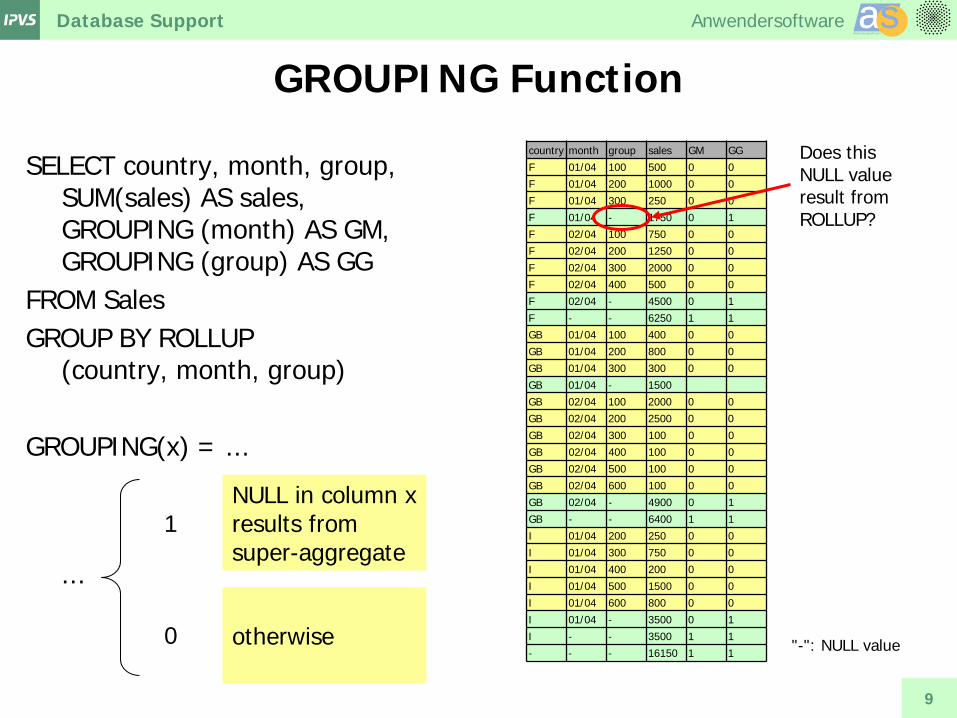
GROUPING Function

SELECT country, month, group, SUM(sales) AS sales, GROUPING (month) AS GM, GROUPING (group) AS GG

FROM Sales GROUP BY ROLLUP

(country, month, group) GROUPING(x) = ...

...

country month group sales GM GG

F 01/04 100 500 0 0

F 01/04 200 1000 0 0

F 01/04 300 250 0 0

F 01/04 - 1750 0 1

F 02/04 100 750 0 0

F 02/04 200 1250 0 0

F 02/04 300 2000 0 0

F 02/04 400 500 0 0

F 02/04 - 4500 0 1

F - - 6250 1 1

GB 01/04 100 400 0 0

GB 01/04 200 800 0 0

GB 01/04 300 300 0 0

GB 01/04 - 1500

GB 02/04 100 2000 0 0

GB 02/04 200 2500 0 0

GB 02/04 300 100 0 0

GB 02/04 400 100 0 0

GB 02/04 500 100 0 0

GB 02/04 600 100 0 0

GB 02/04 - 4900 0 1

GB - - 6400 1 1

I 01/04 200 250 0 0

I 01/04 300 750 0 0

I 01/04 400 200 0 0

I 01/04 500 1500 0 0

I 01/04 600 800 0 0

I 01/04 - 3500 0 1

I - - 3500 1 1

- - - 16150 1 1 "-": NULL value

Does this NULL value result from ROLLUP?

NULL in column x results from super-aggregate

1

0 otherwise


ss

10

CUBE

• Support for Roll-up (dimension reduction)

• Compute: Sales for all aggregation

groups of attributes country, month and group.

SELECT country, month, group, SUM(sales) FROM Sales GROUP BY GROUPING SETS ( (country, month, group), (country, month), (country, group), (month, group), (country), (month), (group), () ) GROUP BY country, month, group GROUP BY country, group GROUP BY country, month GROUP BY month, group GROUP BY country GROUP BY month GROUP BY group

...

Time

year month day

2002

country region shop#

Germany

Sales query using grouping sets


ss

11

CUBE

SELECT country, month, group,

SUM(sales) FROM Sales GROUP BY CUBE

(country, month, group)


F 01/04 100 500

F 01/04 200 1000

F 01/04 300 250

F 01/04 - 1750

F 02/04 100 750

F 02/04 200 1250

F 02/04 300 2000

F 02/04 400 500

F 02/04 - 4500

F - - 6250

GB 01/04 100 400

GB 01/04 200 800

GB 01/04 300 300

GB 01/04 - 1500

GB 02/04 100 2000

GB 02/04 200 2500

GB 02/04 300 100

GB 02/04 400 100

GB 02/04 500 100

GB 02/04 600 100

GB 02/04 - 4900

GB - - 6400

I 01/04 200 250

I 01/04 300 750

I 01/04 400 200

I 01/04 500 1500

I 01/04 600 800

I 01/04 - 3500

I - - 3500

- - - 16150


F - 100 1250

F - 200 2250

F - 300 2250

F - 400 500

GB - 100 2400

GB - 200 3300

GB - 300 400

GB - 400 100

GB - 500 100

GB - 600 100

I - 200 250

I - 300 750

I - 400 200

I - 500 1500

I - 600 800

- 01/04 100 900

- 01/04 200 2050

- 01/04 300 1300

- 01/04 400 200

- 01/04 500 1500

- 01/04 600 800

- 02/04 100 2750

- 02/04 200 3750

- 02/04 300 2100

- 02/04 400 600

- 02/04 500 100

- 02/04 600 100

- 01/04 - 6750

- 02/04 - 9400

- - 100 3650

- - 200 5800

- - 300 3400

- - 400 800

- - 500 1600

- - 600 900

+

"-": NULL value

equivalent query using CUBE


ss

12

Syntax: Cube and Rollup

<group by clause> ::= GROUP BY <grouping specification>

<grouping specification> ::= <grouping column reference> | <rollup list> | <cube list> | <grouping sets specification> | <grand total> | <concatenated grouping>

<rollup list> ::= ROLLUP ( <grouping column reference list> )

<cube list> ::= CUBE ( <grouping column reference list> )

<grouping sets specification> ::= GROUPING SETS ( <grouping set list> )

<grouping set list> ::= <grouping set> [ { <comma> <grouping set> } … ]

<concatenated grouping> ::= <grouping set> <comma> <grouping set list>

<grouping set> ::= <ordinary grouping set> | <rollup list> | <cube list> | <grand total>

<ordinary grouping set> ::= <grouping column reference> | ( <grouping column reference list> )

<grand total> ::= ( )

<grouping column reference list> ::= <grouping column reference> [ {<comma> <grouping column reference> } … ]

<grouping column reference> ::= <column reference> [ <collate clause> ]

(Source: [MS02])


ss

13

WINDOW

• User-defined selection of rows within a query.

• Perform calculations with respect to the current row and the window defined.

• Example: Calculate the sum of sales

for each month and the two preceding months; provide the sum per country and group.

Sales country month group sales

F 01/04 100 500

F 02/04 100 1000

F 03/04 100 250

F 04/04 100 750

F 02/04 200 1250

F 03/04 200 2000

F 04/04 200 500

GB 01/04 100 400

GB 02/04 100 800

GB 03/04 100 300

GB 04/04 100 2000

GB 05/04 100 2500

GB 02/04 200 100

GB 03/04 200 100

GB 04/04 200 100

GB 05/04 200 100

I 01/04 300 250

I 02/04 300 750

I 03/04 300 200

I 04/04 300 1500

I 05/04 300 800

window partitioning

window ordering

window framing

500

1750 2000

1500


ss

14

WINDOW

SELECT country, month, group, sales, SUM(sales) OVER w AS moving_sum

FROM Sales AS s WINDOW w AS ( PARTITION BY s.country, s.group ORDER BY s.month ROWS 2 PRECEDING ) SELECT country, month, group, sales,

SUM(sales) OVER ( PARTITION BY s.country,

s.group ORDER BY s.month ROWS 2 PRECEDING )

AS moving_sum FROM Sales AS s

country month group sales moving_sum

F 01/04 100 500 500

F 02/04 100 1000 1500

F 03/04 100 250 1750

F 04/04 100 750 2000

F 02/04 200 1250 1250

F 03/04 200 2000 3250

F 04/04 200 500 3750

GB 01/04 100 400 400

GB 02/04 100 800 1200

GB 03/04 100 300 1500

GB 04/04 100 2000 3100

GB 05/04 100 2500 4800

GB 02/04 200 100 100

GB 03/04 200 100 200

GB 04/04 200 100 300

GB 05/04 200 100 300

I 01/04 300 250 250

I 02/04 300 750 1000

I 03/04 300 200 1200

I 04/04 300 1500 2450

I 05/04 300 800 2500

window partitioning

window ordering

window framing

in-line window specification


ss

15

WINDOW Ordering

• Specifies the ordering for each of the partitions.

• NULLS FIRST: All NULL values appear first in the ordering - regardless of whether you specify ASC or DESC

• similar for NULLS LAST • <null ordering> is provided for

WINDOW ordering only.

• Without <null ordering> clause: Null values are sorted as though they were less than all non-null values, or as they were greater than all non-null values. The choice is implementation-defined.

• Window ordering has no influence on the order of rows that are returned.

ORDER BY <sort specification> [ { <comma> <sort specification> } … ] <sort specification> :: = <sort key> [ <ordering specification> ] [ <null ordering> ] <ordering specification> ::= ASC | DESC <null ordering> ::= NULLS FIRST | NULLS LAST


ss

16

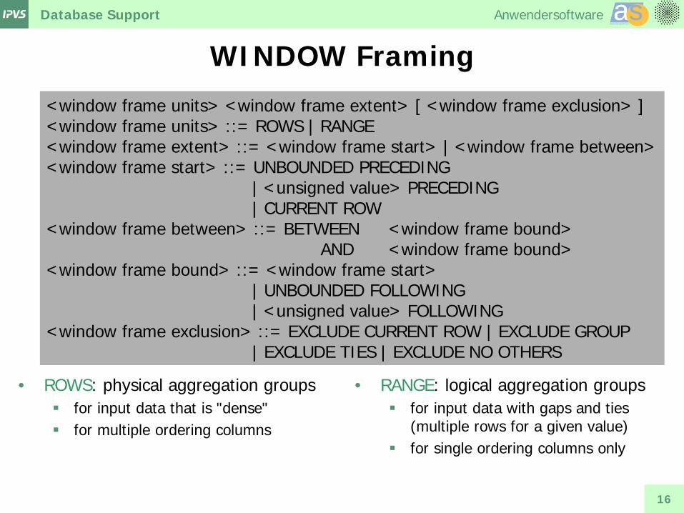
WINDOW Framing

• ROWS: physical aggregation groups for input data that is "dense" for multiple ordering columns

• RANGE: logical aggregation groups for input data with gaps and ties

(multiple rows for a given value) for single ordering columns only

<window frame units> <window frame extent> [ <window frame exclusion> ] <window frame units> ::= ROWS | RANGE <window frame extent> ::= <window frame start> | <window frame between> <window frame start> ::= UNBOUNDED PRECEDING | <unsigned value> PRECEDING | CURRENT ROW <window frame between> ::= BETWEEN <window frame bound> AND <window frame bound> <window frame bound> ::= <window frame start> | UNBOUNDED FOLLOWING | <unsigned value> FOLLOWING <window frame exclusion> ::= EXCLUDE CURRENT ROW | EXCLUDE GROUP | EXCLUDE TIES | EXCLUDE NO OTHERS


ss

17

WINDOW Framing

… ORDER BY month RANGE BETWEEN INTERVAL '1' MONTH PRECEDING AND INTERVAL '1' MONTH FOLLOWING

/* logical aggregation group including the last, current, and next month */ … ORDER BY month ROWS BETWEEN 1 PRECEDING AND 1 FOLLOWING /* physical aggregation group on a dense column */ … ROWS BETWEEN 5 PRECEDING AND CURRENT ROW … ROWS 5 PRECEDING /* preceding 5 rows and current row */ … ROWS UNBOUNDED PRECEDING /* all preceding rows and current row */ … ROWS BETWEEN CURRENT ROW AND UNBOUNDED FOLLOWING /* current row and all following rows */ … ROWS BETWEEN 6 PRECEDING AND 3 PRECEDING /* the 3 rows starting 6 rows before the current row, current row is not

included */


ss

18

OLAP Functions: Numeric Value Functions

• LN (x): Returns the natural logarithm of x. Exception if x is zero or negative.

• EXP (x): Returns the value computed by raising the value of e (the base of natural logarithms) to the power specified by x.

• POWER (x, y): Returns the value computed by raising x to the power of y.

• SQRT (x): Returns the square root of x. = POWER (x, 0.5)

• FLOOR (x): Returns the integer value nearest to positive infinity that is not greater than x.

• CEILING (x): Returns the integer value nearest to negative infinity that is no less than x.

• WIDTH_BUCKET (x, l, r, n): Returns a number indicating the partition into which x should be placed, if the range from l to r is divided into n equal-sized partitions.

x y result

0 0 1

0 >0 0

0 <0 exception

<0 no integer exception


ss

19

OLAP Functions: Ranking

• Sparse ranking: RANK returns a number that indicates the rank of the "current" row among the rows in the row's partition. RANK provides a sparse ranking, i.e., gaps are possible.

• Dense ranking: DENSE_RANK returns a ranking without gaps.

A B

1 10

1 20

1 20

1 20

1 30

1 40

SELECT A, B, RANK OVER (PARTITION BY A ORDER BY B ASC) AS r, DENSE_RANK OVER (PARTITION BY A ORDER BY B DESC) AS dr, FROM T

A B r dr

1 10 1 4

1 20 2 3

1 20 2 3

1 20 2 3

1 30 5 2

1 40 6 1


ss

20


• Relative ranking: provided by PERCENT_RANK: (RANK of row in its partition - 1) / (number of rows in the partition - 1) provided by CUME_DIST: number of rows that precede or peers with the row being examined divided by the total number of rows in the partition.

• Row Number Function: ROW_NUMBER assigns a number to each row, based on its position within its window partition

A B

1 10

1 20

1 20

1 20

1 30

1 40

SELECT A, B, PERCENT_RANK() OVER (PARTITION BY A ORDER BY B ASC) AS pr, CUME_DIST() OVER (PARTITION BY A ORDER BY B ASC) AS cr, ROW_NUMBER() OVER (PARTITION BY A ORDER BY B ASC) AS rn FROM T

A B pr cr rn

1 10 0 0.16 1

1 20 0.2 0.66 2

1 20 0.2 0.66 3

1 20 0.2 0.66 4

1 30 0.8 0.83 5

1 40 1 1 6


ss

21


• Sparse ranking: RANK() OVER ws ⇒ ( COUNT(*) OVER (ws RANGE UNBOUNDED PRECEDING) - COUNT(*) OVER (ws RANGE CURRENT ROW) + 1)

• Dense ranking: DENSE_RANK() ⇒ ( COUNT( DISTINCT ROW (ve1, …, ven)) OVER OVER ws (ws RANGE UNBOUNDED PRECEDING) ve1, …, ven: value expressions in the sort spec. of window ws

• Relative ranking: PERCENT_RANK() ⇒ CASE OVER ws WHEN COUNT(*) OVER (ws RANGE BETWEEN UNBOUNDED PRECEDING AND UNBOUNDED FOLLOWING ) = 1 THEN CAST (0 AS ANT) ELSE (CAST (RANK () OVER (ws) AS ANT ) -1) / (COUNT(*) OVER (ws RANGE BETWEEN UNBOUNDED PRECEDING AND UNBOUNDED FOLLOWING ) -1) CUME_DIST() ⇒ (CAST ( COUNT(*) OVER ws RANGE UNBOUNDED PRECEDING) AS ANT ) / OVER ws COUNT(*) OVER (ws RANGE BETWEEN UNBOUNDED PRECEDING AND UNBOUNDED FOLLOWING )) ANT: any numeric type

• Row number: ROW_NUMBER ⇒ COUNT(*) OVER ws RANGE UNBOUNDED PRECEDING OVER ws


ss

22

Aggregate Functions and the Filter Clause

• FILTER Clause: Allows to specify that the rows of each window partition or grouped table are filtered by a search condition before the specified aggregate function is computed.


F 01/04 100 500

F 01/04 200 1000

F 01/04 300 250

F 02/04 100 750

F 02/04 200 1250

F 02/04 300 2000

F 02/04 400 500

GB 01/04 100 400

GB 01/04 200 800

GB 01/04 300 300

GB 02/04 100 2000

GB 02/04 200 2500

GB 02/04 300 100

GB 02/04 400 100

GB 02/04 500 100

GB 02/04 600 100

I 01/04 200 250

I 01/04 300 750

I 01/04 400 200

I 01/04 500 1500

I 01/04 600 800

SELECT country, COUNT(*) AS count, COUNT(*) FILTER (WHERE sales>1000) AS c2, COUNT(*) FILTER (WHERE group=600) AS c3 FROM Sales GROUP BY country HAVING country <> 'I'

country count c2 c3

F 7 2 0

GB 9 2 1


ss

23

Other OLAP Functions

• STDDEV_POP ( value expression): Computes the population standard deviation of the provided expression evaluated for each row of the group or partition1, defined as the square root of the population variance.

• STDDEV_SAMP (value expression): Computes the sample standard deviation of the provided expression evaluated for each row of the group or partition1, defined as the square root of the sample variance.

1if DISTINCT was specified, each row that remains after duplicates have been eliminated.

• VAR_POP (value expression): Computes the population variance of expression evaluated for each row of the group or partition1, defined as the sum of squares of the difference of expression from the mean of expression, divided by the number of rows in the group or partition.

• VAR_SAMP (value expression): Computes the sample variance of expression evaluated for each row of the group or partition1, defined as the sum of squares of the difference of expression from the mean of expression, divided by one less than the number of rows in the group or partition.


ss

24

Other OLAP Functions

• COVAR_POP (expr1, expr2): Computes the population covariance.

• COVAR_SAMP (expr1, expr2): Computes the sample covariance.

• CORR (expr1, expr2): Computes the correlation coefficient.

• REGR_SLOPE (expr1, expr2): Computes the slope of the least-squares-fit linear equation.

• REGR_INTERCEPT (expr1, expr2): Computes the y-intercept of the least-squares-fit linear equation.

• REGR_COUNT (expr1, expr2): Computes the number of rows remaining in the group or partition.

• REGR_R2 (expr1, expr2): Computes the square of the correlation coefficient.

• REGR_AVGX (expr1, expr2): Computes the average of expr2 for all rows in the group or partition.

• REGR_AVGY (expr1, expr2): Computes the average of expr1 for all rows in the group or partition.

• REGR_SXX (expr1, expr2): Computes the sum of squares of expr2 for all rows in the group or partition.

• REGR_SYY (expr1, expr2): Computes the sum of squares of expr1 for all rows in the group or partition.

• REGR_SXY (expr1, expr2): Computes the sum of products of expr2 times expr1 for all rows in the group or partition.


ss

25

Overview






ss

26

SQL/MM Part 6: Data Mining

• SQL/MM: Multimedia and Application Packages Part 6 falls into the "applications packages" because it does not address "multimedia" data but deals with models and algorithms on data through the use of SQL:1999 user-defined types.

• Supported data mining techniques: association rules clustering regression classification

• SQL/MM Data Mining defines types and routines that allow to specify data sets for mining tasks specify mining tasks derive, test, and apply data mining models import and export mining models


ss

27

Object-Oriented Extensions in SQL:1999

• User-defined structured types Type hierarchy supported Type-specific behaviour may be specified as methods Structured types may be used in

- Column definitions - Table definitions - View definitions

• Typed tables and typed views Tables and views each of whose rows is an instance of a structured

type Table hierarchy or view hierarchy supported Reference types allow navigational access


ss

28

User-Defined Structured Types

• Example: Type hierarchy

CREATE TYPE colored_part_t UNDER part_t AS ( color_id INT) NOT FINAL

CREATE TYPE part_t AS ( partno CHAR(4), version VARCHAR(10), projectno CHAR(4), description VARCHAR(50)) REF USING INT

inherits all components of type part

objects are identified by integer values


ss

29

Typed Tables

• Example: Table hierarchy based on a type hierarchy CREATE TABLE parts OF part_t ( partno WITH OPTIONS NOT NULL, version WITH OPTIONS NOT NULL, projectno WITH OPTIONS NOT NULL, REF IS oid USER GENERATED)

CREATE TABLE colored_parts OF colored_part_t UNDER parts INHERIT SELECT PRIVILEGES ( color_id WITH OPTIONS NOT NULL)

column constraints

Define the self referencing column oid which contains in each row a value that uniquely identifies the row. In this case the identifier is provided by the user.

oid partno version projectno description

1 P050 1.0 PJ23 bodywork

… … … … …

oid partno version projectno description color_id

10 P102 1.2 PJ23 a column 117

… … … … …

parts

colored_parts


ss

30

User-Defined Methods

• Example: Method definition

• Example: Method usage

CREATE METHOD next_color (n INT) RETURNS INT FOR colored_part_t RETURN SELF.color_id + n

SELECT partno, color_id, DEREF(oid).next_color(1) AS next FROM colored_parts

oid partno version projectno description color_id

10 P102 1.2 PJ23 a column 117

… … … … …

colored_parts

partno color_id next

P102 117 118

…


ss

31

Data Mining Phases

• The training phase generates a data mining model. • The test phase consumes a set of tuples carrying values in a special field.

Each tuple is evaluated by the data mining model. Then, the predicted value of the special field is compared to the actual value.

• During the application phase each given tuple is evaluated by the model and one or more values are computed (cluster-ID for clustering, a predicted value for classification or regression).

Data mining technique Training phase

Test phase

Application phase

Classification Regression Clustering Association rule discovery


ss

32

Data Mining Types

Types Category Purpose

DM_RuleModel DM_ClusteringModel

DM_RegressionModel DM_ClasModel

Data mining models

Represents models that are the result of a data mining step

DM_RuleSettings DM_ClusSettings

DM_RegSettings DM_ClasSettings

Data mining settings

Describes the settings that are used to generate a model

DM_RuleTask DM_ClusTask

DM_RegTask DM_ClasTask

Data mining settings

Represents the information about a model generation task

DM_ClusResult DM_RegResult

DM_ClasResult Data mining application results

Describes the results of an application run of a data mining model

DM_RegTestResult DM_ClasTestResult

Data mining test results

Describes the results of a test run of a data mining model

DM_LogicalDataSpec DM_MiningData DM_ApplicationData

Data mining data

Describes the data sets for training, testing, and application


ss

33

DM_ClasModel Type and Routines

CREATE TYPE DM_ClasModel AS ( DM_content CHARACTER LARGE OBJECT(DM_MaxContentLength)) INSTANTIABLE NOT FINAL STATIC METHOD DM_impClasModel (input CHARACTER LARGE OBJECT (DM_MaxContentLength)) RETURNS DM_ClasModel LANGUAGE SQL DETERMINISTIC CONTAINS SQL RETURNS NULL ON NULL INPUT, METHOD DM_expClasModel() RETURNS CHARACTER LARGE OBJECT(DM_MaxContentLength) LANGUAGE SQL DETERMINISTIC CONTAINS SQL, METHOD DM_clasGetTask() RETURNS DM_ClasTask LANGUAGE SQL DETERMINISTIC CONTAINS SQL,

METHOD DM_clasCostRate() RETURNS DOUBLE LANGUAGE SQL DETERMINISTIC CONTAINS SQL, METHOD DM_clasModelSchema() RETURNS DM_MiningSchema LANGUAGE SQL DETERMINISTIC CONTAINS SQL, METHOD DM_applyClasModel (input DM_ApplicationData) RETURNS DM_ClasResult LANGUAGE SQL DETERMINISTIC CONTAINS SQL RETURNS NULL ON NULL INPUT, METHOD DM_testClasModel (input DM_MiningData) RETURNS DM_ClasTestResult LANGUAGE SQL DETERMINISTIC CONTAINS SQL RETURNS NULL ON NULL INPUT


ss

34

Sample Classification

Application scenario • Given: A customer table CT of an insurance company with

columns C1, C2, …, C9: contain characteristics of customers

column r: contains the risk class of each customer (e.g. 'low', 'medium', 'high')

• Objectives: Compute a classification model that allows to predict the risk for a

new customer. It should be possible to re-compute the classification model from time

to time to see whether the model changes over time. It must be possible to test a classification model with a given test

table TT also containing columns C1, C2, …, C9 and r.

C1 C2 … C9 r

CT


ss

35

Classification: Phases and Types

DM_ClasTask

DM_ClasTestResult

DM_ClasResult

DM_MiningData

DM_ApplicationData

DM_ClasModel training

application

test

DM_MiningData


ss

36

Create a Mining Task

• The DM_ClasTask value has to be stored to be able to run the data mining training several times. Table MT is used for this purpose.

• Main steps: Create a DM_MiningData value using

the static method DM_defMiningData. Create a DM_MiningSchema value

using the method DM_genMiningSchema of the DM_MiningData value.

Create a DM_ClasSettings value using the default constructor DM_ClasSettings and assign the DM_MiningSchema value as the schema to use.

Declare the column named ‘r’ as the predicted field using the DM_clasSetTarget method.

Create a DM_ClasTask value using the DM_defClasTask method.

Store the newly created DM_ClasTask value in table MT.

WITH MyData AS (DM_MiningData::DM_defMiningData('CT')) INSERT INTO MT (ID, TASK) VALUES (1, DM_ClasTask::DM_defClasTask( MyData, NULL, ( (new DM_ClasSettings()).DM_clasUseSchema(MyData.DM_genMiningSchema()) ).DM_clasSetTarget(‘r’) ) )


ss

37

Training and Test Phase

• Now that the DM_ClasTask value is generated and stored in the MT table, the classification training can be initiated and the classification model is computed.

• Since the model shall be used in later application and test runs, it is stored in a table MM having two columns ID of type integer and MODEL of type DM_ClasModel.

• A simple test of the model can be done using the data in table TT.

• The result of the test run is of type DM_ClasTestResult.

• DM_ClasTestResult provides a method DM_getClasError() that allows to derive the number of false classifications computed during a test of a classification model.

INSERT INTO MM (ID, MODEL) VALUES ( 1, MyTask.DM_buildClasModel() )

SELECT MODEL.DM_testClasModel( DM_MiningData::DM_defMiningData(‘TT’)) FROM MM WHERE ID = 1


ss

38

Application Phase

• In this example the table used to train the model is again used for an application of the model.

• Method DM_applyClasModel returns the result of applying the classification model contained in MyModel to a given value of DM_ApplicationData retrieved from table CT.

WITH MyModel AS ( SELECT MODEL FROM MM WHERE ID = 1 ) SELECT C1, C2, C3, C4, C5, C6, C7, C8, C9, MyModel.DM_applyClasModel( DM_ApplicationData::DM_impApplData( ‘<C1>’ + C1 + ‘</C1>’ + ‘<C2>’ + C2 + ‘</C2>’ + ‘<C3>’ + C3 + ‘</C3>’ + ‘<C4>’ + C4 + ‘</C4>’ + ‘<C5>’ + C5 + ‘</C5>’ + ‘<C6>’ + C6 + ‘</C6>’ + ‘<C7>’ + C7 + ‘</C7>’ + ‘<C8>’ + C8 + ‘</C8>’ + ‘<C9>’ + C9 + ‘</C9>’ ) ) FROM CT


ss

39

Overview






ss

40

Levels of Database Support

(Source: [Len03])

base data

materialized views

partitioning

indexes

conceptual schema internal schema

P11

P12

P13

MV3 MV2

R1 R2

B tree

grid file

bitmap index

UB tree

R tree

MV1

γ


ss

41

Partitioning

• A table is split into several partitions. • The content of the table is provided by

combining the content of all partitions. • Support for data warehousing:

management of huge data sets

efficient query processing

intra-query-parallelism

01/0

6

03/0

6

03/0

5

04/0

5

…

02/0

6

• rolling data warehouse scenario

• add and drop partitions • add table as partition

• partition pruning • parallel hash joins

01/0

6

03/0

6

03/0

5

04/0

5

…

02/0

6

skip partitions

query

01/0

6

03/0

6

03/0

5

04/0

5

…

02/0

6

query


ss

42

Partitioning Methods

• horizontal partitioning vs. vertical partitioning

• range partitioning: each row is assigned to a certain

partition according to the value of its partitioning attribute

CREATE TABLE TPCH.LINEITEM ( L_ORDERKEY INTEGER NOT NULL, L_PARTKEY INTEGER NOT NULL, L_SUPPKEY INTEGER NOT NULL, … L_SHIPDATE DATE NOT NULL, … PARTITION BY RANGE (L_SHIPDATE) ( PARTITION LINEITEM032005 VALUES LESS THAN '2005-04-01'), ( PARTITION LINEITEM042005 VALUES LESS THAN '2005-05-01'), ( PARTITION LINEITEM052005 VALUES LESS THAN '2005-06-01'), ( PARTITION LINEITEM062005 VALUES LESS THAN '2005-07-01'), … (Oracle)

01/0

6

03/0

6

03/0

5

04/0

5

…

02/0

6

TPCH.LINEITEM


ss

43

Partitioning Methods

• hash partitioning: each row is assigned to a certain

partition according to the value of a linear hash function applied to the partitioning attribute(s) x: h(x) := x mod p p: number of partitions

• combinations: e.g., range partitioning on the

first level and hash partitioning on the second level

CREATE TABLE TPCH.LINEITEM ( L_ORDERKEY INTEGER NOT NULL, L_PARTKEY INTEGER NOT NULL, L_SUPPKEY INTEGER NOT NULL, … L_SHIPDATE DATE NOT NULL, … PARTITION BY HASH (L_ORDERKEY, L_PARTKEY, L_SUPPKEY) PARTITIONS 4 … (Oracle)


ss

44

Overview






ss

45

Materialized Summary Data

• Detailed data as well as summarized data are physically stored in the data warehouse.

• Advantages: Performance enhancement for

queries that access summarized data.

• Challenges: How to identify the suitable set of

materialized summary data? How to efficiently refresh

materialized summary data? How to use summary data

implicitly?


F 01/04 100 500

F 02/04 100 1000

F 03/04 100 250

F 04/04 100 750

F 05/04 200 1250

F 02/04 200 2000

F 03/04 200 500

GB 01/04 100 400

GB 02/04 100 800

GB 03/04 100 300

GB 04/04 100 2000

GB 05/04 100 2500

GB 02/04 200 100

GB 03/04 200 100

GB 04/04 200 100

GB 05/04 200 100

I 01/04 300 250

I 02/04 300 750

I 03/04 300 200

I 04/04 300 1500

I 05/04 300 800

Sales_per_country country sales

F 6250

GB 6400

I 3500

aggregation


ss

46

Types of Summary Data

• Classification based on operations

• Other important characteristics: Linkage between detailed data and summary data Responsibility for refreshing summary data Usage of summary data in query processing

γ γ

MJ view MA view MAJ view


ss

47

Explicit vs. Implicit Summary Data

Explicit Summary Data • Provided as additional tables

no link to detailed data

• Refreshing summary data: part of ETL processing

• Usage: Applications include queries that:

- refer to detailed data - refer to summary data

Implicit Summary Data • Provided by materialized views

materialized view is linked to detailed data

• Refreshing summary data: part of updates on detailed data DB system is responsible for

refreshing

• Usage: Applications include queries that:

- always refer to detailed data

DB system automatically rewrites the query to allow usage of summary data.


ss

48

Explicit Summary Data


F 01/04 100 500

F 02/04 100 1000

F 03/04 100 250

F 04/04 100 750

F 05/04 200 1250

F 02/04 200 2000

F 03/04 200 500

GB 01/04 100 400

GB 02/04 100 800

GB 03/04 100 300

GB 04/04 100 2000

GB 05/04 100 2500

GB 02/04 200 100

GB 03/04 200 100

GB 04/04 200 100

GB 05/04 200 100

I 01/04 300 250

I 02/04 300 750

I 03/04 300 200

I 04/04 300 1500

I 05/04 300 800


F 6250

GB 6400

I 3500

SELECT month, SUM(sales) FROM Sales WHERE group = 100 GROUP BY month

SELECT country, SUM(sales) FROM Sales_per_country WHERE country<>'I' GROUP BY country

query summary data

ETL processing


ss

49


Sales region_dim

region_type

time_dim time_type customer_dim

customer_type

sales

50 1 401 3 10501 1 500

50 1 402 3 10501 1 1000

50 1 403 3 10501 1 250

50 1 404 3 10501 1 750

50 1 402 3 10502 1 1250

50 1 403 3 10502 1 2000

50 1 405 3 10502 1 500

51 1 401 3 10501 1 400

51 1 402 3 10501 1 800

51 1 403 3 10501 1 300

51 1 404 3 10501 1 2000

51 1 405 3 10501 1 2500

51 1 402 3 10502 1 100

51 1 403 3 10502 1 100

51 1 404 3 10502 1 100

51 1 405 3 10502 1 100

53 1 401 3 10505 1 250

53 1 402 3 10505 1 750

53 1 403 3 10505 1 200

53 1 404 3 10505 1 1500

53 1 405 3 10505 1 800

50 1 2004 4 100 2 6250

51 1 2004 4 100 2 6400

53 1 2004 4 100 2 3500

Region Dimension region_type

country_id country_desc

region_id region_desc

1 50 F 70 EU

1 51 GB 70 EU

1 53 I 70 EU

2 - - 70 EU

...

Time Dimension time_type

month_id month_desc

year_id year_desc

...

...

3 401 01/04 2004 2004

3 402 02/04 2004 2004

3 403 03/04 2004 2004

3 404 04/04 2004 2004

3 405 05/04 2004 2004

...

4 - - 2004 2004

...

Customer Dimension

customer_type

customer_id customer_desc

group_id group_desc ...

...

1 10501 name1 100 key cust.



...

2 - - 100 key cust.

...

1: day

2: week

time dimension

3: month

4: year

1: country

2: region

region dimension

3: all

1: customer

2: group

customer dimension

3: all

Fact table contains materialized summary

data


ss

50


SELECT T.month_desc, SUM(S.sales) FROM Sales S, Time T WHERE S.customer_dim = 10501 AND S.region_type = 1 AND S.time_type = 3 AND S.customer_type = 1 AND S.time_type = T.time_type AND S.time_dim = T.month_id GROUP BY T.month_desc

SELECT R.country_desc, T.year_desc, C.group_desc, SUM(S.sales) FROM Sales S, Region R, Time T, Customer C WHERE R.country_desc<>'I' AND S.region_type = 1 AND S.time_type = 4 AND S.customer_type = 2 AND S.region_type = R.region_type AND S.region_dim = R.country_id AND S.time_type = T.time_type AND S.time_dim = T.year_id AND S.customer_type = C.customer_type AND S.customer_dim = C.group_id GROUP BY R.country_desc, T.year_desc, C.group_desc

country_desc

year_desc

group_desc sales

F 2004 key cust. 6250

GB 2004 key cust. 6400

month_desc

sales

01/04 900

02/04 1800

03/04 550

04/04 2750

05/04 2500


ss

51

Implicit Summary Data


F 01/04 100 500

F 02/04 100 1000

F 03/04 100 250

F 04/04 100 750

F 05/04 200 1250

F 02/04 200 2000

F 03/04 200 500

GB 01/04 100 400

GB 02/04 100 800

GB 03/04 100 300

GB 04/04 100 2000

GB 05/04 100 2500

GB 02/04 200 100

GB 03/04 200 100

GB 04/04 200 100

GB 05/04 200 100

I 01/04 300 250

I 02/04 300 750

I 03/04 300 200

I 04/04 300 1500

I 05/04 300 800


F 6250

GB 6400

I 3500

SELECT month, SUM(sales) FROM Sales WHERE group = 100 GROUP BY month

SELECT country, SUM(sales) FROM Sales WHERE country<>'I' GROUP BY country

query detailed data

db system internally uses summary

automatic refresh


ss

52

Derivability

• Problem statement: Given a query Q and a set of summary data M. Under which conditions is the result of Q derivable from M?

• Aspects of derivability: predicates aggregate functions base tables groupings

• Knowledge on derivability is used in two ways: processing of query Q: decide whether M can be used or not selecting the most appropriate summary data


ss

53

Derivability and Predicates

• PQ predicate of query Q, PM predicate of summary data M • Conditions for derivability:

all attributes of PQ are provided by M PQ ⊆ PM

• Example:

CREATE VIEW Sales_per_country_month SELECT country, month, SUM(sales) AS sales FROM Sales GROUP BY country, month

Query Summary Data

SELECT country, SUM(sales) FROM Sales WHERE country<>'I' GROUP BY country


ss

54

Classification of Aggregate Functions

Additive aggregate functions: • Conditions:

F(x1∪x2)=F(F(x1),F(x2)) F-1() exists

Semi-additive aggregate functions: • Conditions:

F(x1∪x2)=F(F(x1),F(x2))

Additive-computable functions: • Conditions:

F(x)=G(F1(x), ..., Fn(x) where G is a algebraic expression and Fi are additive or semi- additive aggregate functions

aggregate functions

additive-computable aggregate functions

semi-additive aggregate functions

additive aggregate functions

Median

STDDEV

VARIANCE

COVARIANCE

AVG

MAX MIN

COUNT

SUM


ss

55

Derivability and Aggregate Functions

• Additive aggregate function: is used in query Q and in summary data M Q is derivable from M

• Semi-additive aggregate function: is used in query Q and in summary data M Q is derivable from M incremental refreshing of M not possible for DELETE operations

• Additive-computable aggregate functions: is used in query Q and based on additive or semi-additive functions

used in M Q is derivable from M incremental refreshing of M not possible for DELETE operations

• All other aggregate functions: no derivability


ss

56

Derivability and Base Tables

• Summary data M includes a join on tables A and B and a join predicate PAB.

• Condition for derivability: Query Q is derivable from M if Q also includes a join on tables A and B

and the join predicate PAB. • Condition can be relaxed:

based on assertions on the data warehouse schema

e.g., if A and B build a lossless join, B is not necessary in query Q.

A B

M

Query Q: SELECT ... FROM A WHERE ...

Cannot be derived from M


ss

57

Derivability and Groupings

• Gi={A1, ..., An) is a grouping with grouping attributes A1, .., An and

• Grouping G2 is directly derivable from G1 if one of the following conditions holds: the grouping attributes of G2 contain the grouping attributes of G1

except one, i.e., G2 ⊂ G1 and exactly one grouping attribute Ak of G1 is replaced in G2 by another

attribute Ao such that Ak→Ao.

• An acyclic dependency graph is build from groupings that are directly derivable.

• Grouping G2 is derivable from G1 if a path from G1 to G2 exists in the dependency graph (G1<G2).

• A grouping set is derivable from grouping set if each grouping of GS2 is derivable from at least one grouping of GS1.

)AA(:lk,nl,k1l,k lk →¬≠≤≤∀

1GG 12 −=

}G,...,G{GS 2m

212 =

}G,...,G{GS 1n

111 =


ss

58

Sample Dependency Graph

G1={A,B,C,D,E,F}

G3={B,C,D,F}

G2={B,C,D,E,F}

G4={B,C,G,E,F}

GS1

GS2

directly derivable


ss

59

Sample Dependency Graph

G1={A,B,C,D,E,F}

G3={B,C,D,F}

G2={B,C,D,E,F}

G4={B,C,G,E,F}

materialized groupings

queried groupings


ss

60

Number of Groupings

• The number of groupings that have to be considered for materialized summary data grows exponentially with the number of available grouping attributes.

• For n attributes, 2n groupings have to be considered: 3 attributes → 8 combinations 10 attributes → 1024 combinations 25 attributes → 33554432 combinations


ss

61

Groupings and Sparsity

• Density of summary data depending on aggregation factor and density of base data

(Source: [Len03])

0

100

200

300

400

500

600

700

800

900

1000

2 3 4 5 6 7 8

number of dimensions

grow

th in

%

• Growth of data volume density: 2%; aggregation factor 1:20

0

0,2

0,4

0,6

0,8

1

1,2

0,10%

0,20%

0,40%

0,80%

1,60%

3,20%

6,70%

14,30

%

25,00

%

33,30

%

50,00

%

100,0

0%

aggregation factor of summary data

dens

ity o

f sum

mar

y da

ta

0,5%1,0%2,0%5,0%10,0%

density of base data


ss

62

Materialized View Selection Approaches

static dynamic

based on benefit

based on refreshing cost

based on multi-query graph

.


ss

63

Materialized View Selection

• Set of n queries (workload): Q={q1, … ,qn} • Set of m materialized views: M={v1, … vm}

• Execution cost for query q based on materialized view v: • Execution cost for query q based on materialized views M:

• Frequency of query qi in workload: fi • Execution cost for all queries in Q based on materialized views M:

• Benefit of additional materialized views u1, ..., uk:

)),((min),( vqCMqCMv∈

=

),( vqC

∑∈

⋅=Qq

iii

MqCfMQC ),(),(

}),...,{,(),()},,...,({ 11 kk uuMQCMQCMuuB ∪−=


ss

64

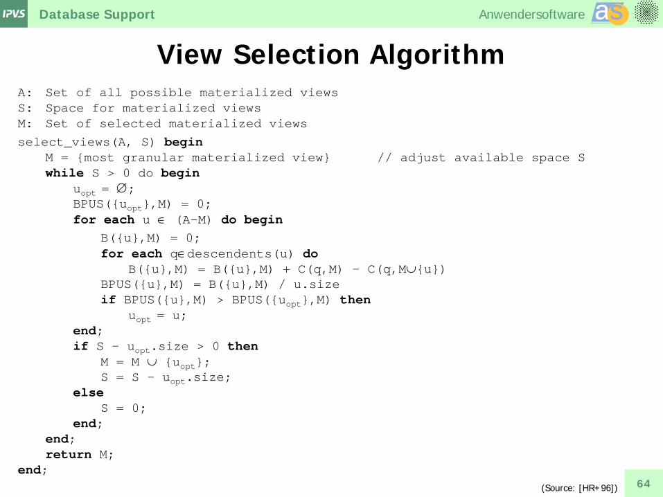
View Selection Algorithm A: Set of all possible materialized views S: Space for materialized views M: Set of selected materialized views

select_views(A, S) begin M = {most granular materialized view} // adjust available space S while S > 0 do begin uopt = ∅; BPUS({uopt},M) = 0; for each u ∈ (A-M) do begin B({u},M) = 0; for each q∈descendents(u) do B({u},M) = B({u},M) + C(q,M) - C(q,M∪{u}) BPUS({u},M) = B({u},M) / u.size if BPUS({u},M) > BPUS({uopt},M) then uopt = u; end; if S - uopt.size > 0 then M = M ∪ {uopt}; S = S - uopt.size; else S = 0; end; end; return M; end;

(Source: [HR+96])


ss

65

Example: View Selection Algorithm

• Possible groupings and their cardinality.

• Cardinality reflects the query execution cost.


F 01/04 100 500

F 02/04 100 1000

F 03/04 100 250

F 04/04 100 750

F 05/04 200 1250

F 02/04 200 2000

F 03/04 200 500

GB 01/04 100 400

GB 02/04 100 800

GB 03/04 100 300

GB 04/04 100 2000

GB 05/04 100 2500

GB 02/04 200 100

GB 03/04 200 100

GB 04/04 200 100

GB 05/04 200 100

I 01/04 300 250

I 02/04 300 750

I 03/04 300 200

I 04/04 300 1500

I 05/04 300 800

grouping cardinality

none 1

C 150

M 3

G 5

C, M 450

C, G 750

M, G 15

C, M, G 2250

(C, M, G)2250

(C, M)450 (C, G)750 (M, G)15

(C)150 (M)3 (G)5

()1


ss

66


• A={(), (C) ,(M) ,(G), (C, M), (C, G), (M, G), (C, M, G)} S=2300 M={}

• first step: M={(C, M, G)}, S=50

(C, M, G)2250

(C, M)450 (C, G)750 (M, G)15

(C)150 (M)3 (G)5

()1


ss

67

selected


• A={(), (C) ,(M) ,(G), (C, M), (C, G), (M, G), (C, M, G)} S=2300 M={}

• second step: M={(C, M, G),()}, S=49

(C, M, G)2250

(C, M)450 (C, G)750 (M, G)15

(C)150 (M)3 (G)5

()1

u B({u},M) BPUS({u},M)

(C, M) (2250-450)+(2250-450)+ (2250-450)+(2250-450)

16

(C, G) (2250-750)+(2250-750)+ (2250-750)+(2250-750)

8

(M, G) (2250-15)+(2250-15)+ (2250-15)+(2250-15)

596

(C) (2250-150)+(2250-150) 28

(M) (2250-3)+(2250-3) 1498

(G) (2250-5)+(2250-5) 898

() (2250-1) 2249


ss

68


• third step: M={(C, M, G),(),(M)}, S=46 (C, M, G)2250

(C, M)450 (C, G)750 (M, G)15

(C)150 (M)3 (G)5

()1


(C, M) (2250-450)+(2250-450)+ (2250-450) = 5400

12

(C, G) (2250-750)+(2250-750)+ (2250-750) = 4500

6

(M, G) (2250-15)+(2250-15)+ (2250-15) = 6705

447

(C) (2250-150) = 2100 14

(M) (2250-3) = 2247 749

(G) (2250-5) = 2245 449


ss

69


• fourth step: M={(C, M, G),(),(M),(G)}, S=41

(C, M, G)2250

(C, M)450 (C, G)750 (M, G)15

(C)150 (M)3 (G)5

()1


(C, M) (2250-450)+(2250-450) = 1800

4

(C, G) (2250-750)+(2250-750)+ (2250-750) = 4500

6

(M, G) (2250-15)+(2250-15) = 4470

298

(C) (2250-150) = 2100 14

(G) (2250-5) = 2245 449


ss

70


• fifth step: M={(C, M, G),(),(M),(G),(M,G)} S=41

• not enough space for further materialization

• final result: {(), (M), (G), (M, G), (C, M, G)}

(C, M, G)2250

(C, M)450 (C, G)750 (M, G)15

(C)150 (M)3 (G)5

()1


(C, M) (2250-450)+(2250-450) = 1800

4

(C, G) (2250-750)+(2250-750) = 3000

4

(M, G) (2250-15) = 2235 149

(C) (2250-150) = 2100 14


ss

71

View Selection Algorithm (by Size)

A: Set of all possible materialized views S: Space for materialized views M: Set of selected materialized views

select_views_sorted(A, S) begin A = sort_desc_by_size(A); M = {most granular materialized view} while S > 0 do begin umin = min(A); if S - umin.size > 0 then M = M ∪ {umin}; S = S - umin.size; else S = 0; end; end; return M; end;

(Source: [BP+97])


ss

72

Dynamic Approaches

• Static approaches assume a constant query profile for the data warehouse.

• Dynamic approaches: Store query results as materialized summary data

(similar to caching) If not enough space is left

-> choose replacement victim General conditions to be considered in replacement strategies:

- size of materialized summary data - dependencies between materialized summary data - invalidation versus refreshing


ss

73

Refreshing Summary Data

• immediate refresh • on commit refresh • deferred refresh

complete incremental

immediate on-commit deferred

• incremental maintenance (self maintainability required)

• complete refresh

(Source: [Len03])


ss

74

Overview






ss

75

Scan

• All rows of a relation are stored in blocks on external memory: hard drive RAID …

• Table scan

• Scan operation: Retrieve all rows of a table that satisfy a predicate.

• Index scan

retrieve all blocks of the table

extract all rows

apply predicate to each row

use index to identify rows satisfying the predicate

retrieve all blocks containing at least one relevant row

extract relevant rows


ss

76

Indexes

• Each tuple is identified by a tuple identifier (TID) (also RID = row identifier)

• Indexes support the efficient mapping of attribute values to the corresponding rows in a table.

2004-01-31 2004-02-29 2004-03-31

2004-01-15 2004-01-16 2004-01-17 … TID, TID TID TID, TID …

TID …

TID …

TID …

TID …

TID …

TID …

TID …

TID …

TID …

B-Tree on attribute date

block 324 block 325 block 326


ss

77

Indexes on Dimension Tables

• OLAP-queries typically provide restrictions on dimension attributes.

• index allows to identify qualified rows in a dimension

• problem: low-cardinality dimension

attributes

B-Tree on attribute risk

low medium … TID1, TID2, … TID1, … TID100450 TID50600 …

…


ss

78

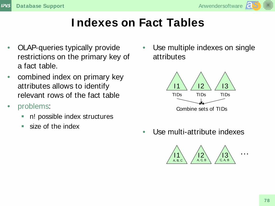
Indexes on Fact Tables

• OLAP-queries typically provide restrictions on the primary key of a fact table.

• combined index on primary key attributes allows to identify relevant rows of the fact table

• problems: n! possible index structures size of the index

• Use multiple indexes on single attributes

• Use multi-attribute indexes

I1 I2 I3 TIDs TIDs TIDs

Combine sets of TIDs

I1

I2

I3 A, B, C C, A, B A, C, B

…


ss

79

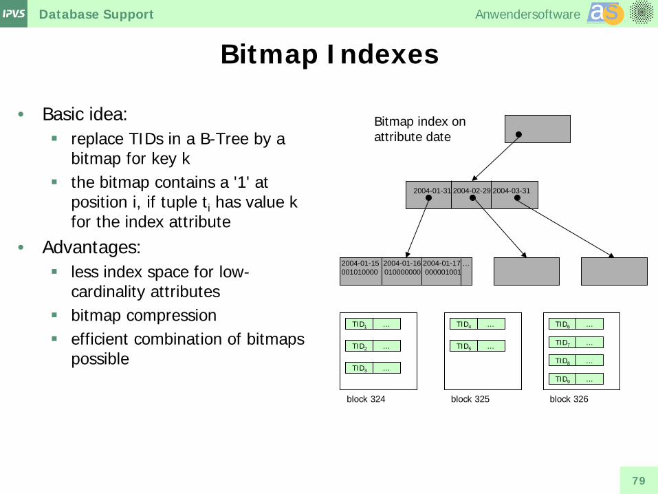
Bitmap Indexes

• Basic idea: replace TIDs in a B-Tree by a

bitmap for key k the bitmap contains a '1' at

position i, if tuple ti has value k for the index attribute

• Advantages: less index space for low-

cardinality attributes bitmap compression efficient combination of bitmaps

possible

2004-01-31 2004-02-29 2004-03-31

2004-01-15 2004-01-16 2004-01-17 … 001010000 010000000 000001001

Bitmap index on attribute date

TID1 …

TID2 …

TID3 …

TID4 …

TID5 …

TID6 …

TID7 …

TID8 …

TID9 …

block 324 block 325 block 326


ss

80

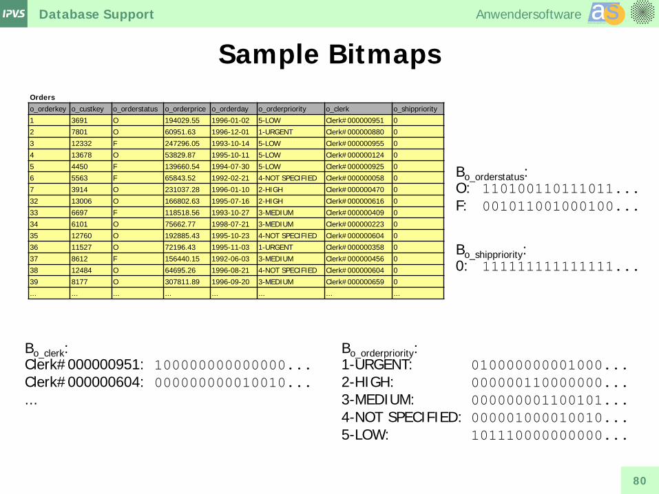
Sample Bitmaps Orders o_orderkey o_custkey o_orderstatus o_orderprice o_orderday o_orderpriority o_clerk o_shippriority

1 3691 O 194029.55 1996-01-02 5-LOW Clerk#000000951 0

2 7801 O 60951.63 1996-12-01 1-URGENT Clerk#000000880 0

3 12332 F 247296.05 1993-10-14 5-LOW Clerk#000000955 0

4 13678 O 53829.87 1995-10-11 5-LOW Clerk#000000124 0

5 4450 F 139660.54 1994-07-30 5-LOW Clerk#000000925 0

6 5563 F 65843.52 1992-02-21 4-NOT SPECIFIED Clerk#000000058 0

7 3914 O 231037.28 1996-01-10 2-HIGH Clerk#000000470 0

32 13006 O 166802.63 1995-07-16 2-HIGH Clerk#000000616 0

33 6697 F 118518.56 1993-10-27 3-MEDIUM Clerk#000000409 0

34 6101 O 75662.77 1998-07-21 3-MEDIUM Clerk#000000223 0

35 12760 O 192885.43 1995-10-23 4-NOT SPECIFIED Clerk#000000604 0

36 11527 O 72196.43 1995-11-03 1-URGENT Clerk#000000358 0

37 8612 F 156440.15 1992-06-03 3-MEDIUM Clerk#000000456 0

38 12484 O 64695.26 1996-08-21 4-NOT SPECIFIED Clerk#000000604 0

39 8177 O 307811.89 1996-09-20 3-MEDIUM Clerk#000000659 0

... ... ... ... ... ... ... ...

Bo_orderstatus: O: 110100110111011... F: 001011001000100...

Bo_orderpriority: 1-URGENT: 010000000001000... 2-HIGH: 000000110000000... 3-MEDIUM: 000000001100101... 4-NOT SPECIFIED: 000001000010010... 5-LOW: 101110000000000...

Bo_shippriority: 0: 111111111111111...

Bo_clerk: Clerk#000000951: 100000000000000... Clerk#000000604: 000000000010010... ...


ss

81

B[i] = BX,D[i]

Bitmap Usage

• using bitmaps for exact match queries: X = D result bitmap B:

• using bitmaps for range queries: X IN(A, B, C, D, E) result bitmap B:

for i=1 to length(BX) B[i] = BX,A[i] OR BX,B[i] OR BX,c[i] OR BX,D[i] OR BX,E[i] ) end for


ss

82

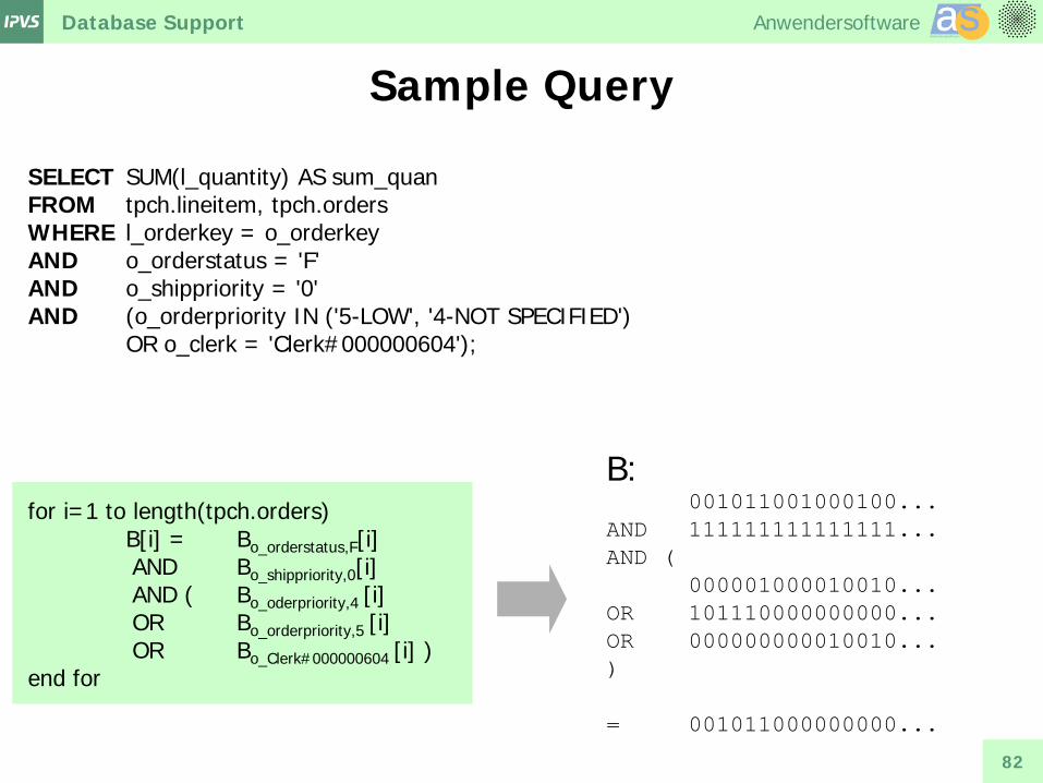
Sample Query

SELECT SUM(l_quantity) AS sum_quan FROM tpch.lineitem, tpch.orders WHERE l_orderkey = o_orderkey AND o_orderstatus = 'F' AND o_shippriority = '0' AND (o_orderpriority IN ('5-LOW', '4-NOT SPECIFIED') OR o_clerk = 'Clerk#000000604'); for i=1 to length(tpch.orders) B[i] = Bo_orderstatus,F[i] AND Bo_shippriority,0[i] AND ( Bo_oderpriority,4 [i] OR Bo_orderpriority,5 [i] OR Bo_Clerk#000000604 [i] ) end for

B: 001011001000100... AND 111111111111111... AND ( 000001000010010... OR 101110000000000... OR 000000000010010... ) = 001011000000000...


ss

83

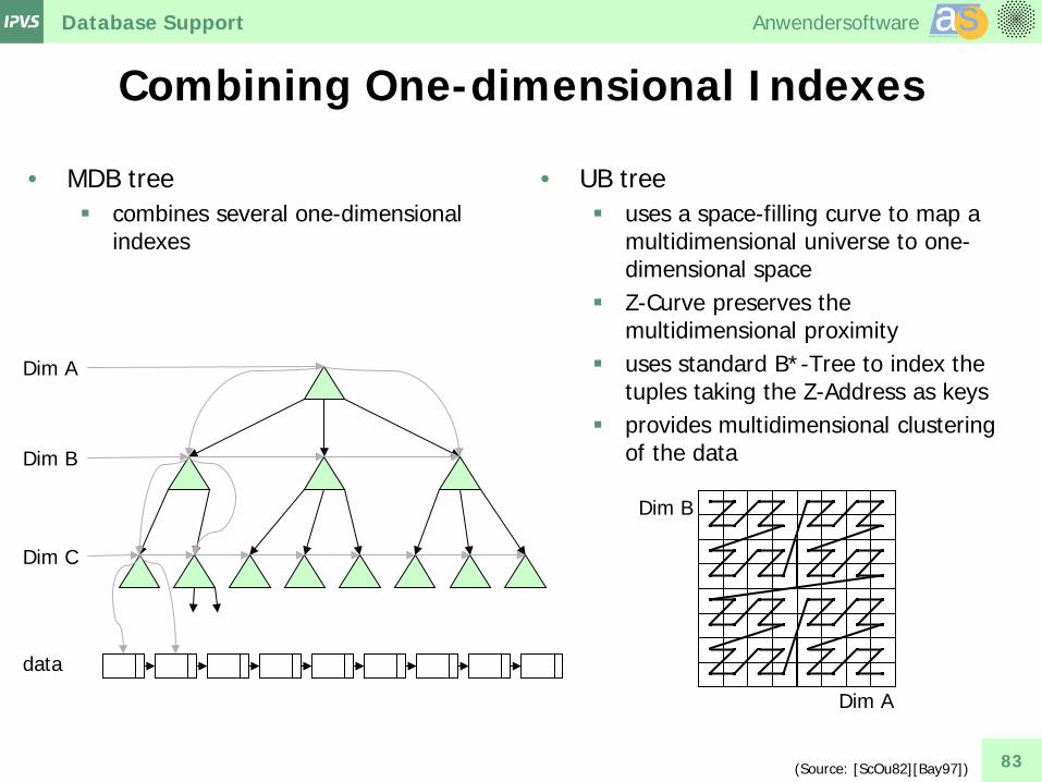
Combining One-dimensional Indexes

• MDB tree combines several one-dimensional

indexes

• UB tree uses a space-filling curve to map a

multidimensional universe to one-dimensional space

Z-Curve preserves the multidimensional proximity

uses standard B*-Tree to index the tuples taking the Z-Address as keys

provides multidimensional clustering of the data

Dim A

Dim B

(Source: [ScOu82][Bay97])

Dim A

Dim B

Dim C

data


ss

84

Multidimensional Indexes

• Symmetric treatment of all dimensions • Examples:

Quadtree (2 dimensions) Octtree (3 dimensions) K-D-B-Tree hB-Tree (holy brick) R-Trees: R-tree, R+-tree, R*-tree, packed R-tree …


ss

85

Overview






ss

86

Star Queries

SELECT D1.a, D2.d, …, Dn.x, f(F.fact) FROM F, D1, D2, …, Dn WHERE F.b = D1.b AND F.e = D2.e … AND D1.c = … AND D2.f = … … GROUP BY D1.a, D2.d, …, Dn.x

• Fact table F • Dimension tables D1, …, Dn • Aggregation f applied to fact

attribute F.fact

• Optimizer has to decide on: join order index usage predicate push-down …

σ1

σ2


ss

87

Evaluating Star Queries

• Basic approach: join fact table and first dimension

table. use index on fact table (join

attribute) if available join result with further dimension

tables until last dimension is reached

• Predicates on dimensions reduce size of intermediate results.

• Join order for dimensions depends on: available indexes selectivity of predicates

D2

Dn-1

Dn

σ2

σn-1

σn

F

D1

σ1

D1

…

γa, d, …, x


ss

88


• Basic approach: join all dimension tables join resulting cartesian

product to the fact table use combined index on fact

table if available

• Reduces size of intermediate results

F

D1 D2

Dn-1

Dn

σ1 σ2

σn-1

σn

D1, …, Dn

…

γa, d, …, x


ss

89


• Basic approach: semi-join of fact table and each

dimension table (results in n sets of TIDs for qualified rows)

index on fact table (join attribute) is mandatory

combine sets of TIDs fetch qualified rows from fact

table join intermediate result with each

dimension table

• Reduces size of intermediate results

• Efficient algorithm needed for intersection of sets of TIDs

D1

D2

Dn

σ1

σ2

σn

γa, d, …, x

F

F D1

D1

σ1

F D2

D2

σ2

F Dn

Dn

σn

AND TIDs

TIDs TIDs

TIDs


ss

90

Join Indexes

• Goal: Provide join between fact table F and dimension table D1 without access to both tables.

• Join Index: Index structure covering the pre-computed join between two tables.

SELECT D1.a, D2.d, …, Dn.x, f(F.fact) FROM F, D1, D2, …, Dn WHERE F.b = D1.b AND F.e = D2.e … AND D1.c = … AND D2.f = … … GROUP BY D1.a, D2.d, …, Dn.x

F D1

D1

σ1

F

D1

σ1

D1 F D1

σ1


ss

91

Join Indexes

F TID b e g

0x100 01/04 100 500

0x101 02/04 100 1000

0x102 03/04 100 250

0x103 04/04 100 750

0x104 05/04 200 1250

0x105 02/04 200 2000

0x106 03/04 200 500

0x107 01/04 100 400

0x108 02/04 100 800

0x109 03/04 100 300

0x110 04/04 100 2000

0x111 05/04 100 2500

0x112 02/04 200 100

D1 TID a b c

0x200 01.01.2004 01/04 Jan

0x201 01.02.2004 02/04 Feb

0x202 01.03.2004 03/04 Mar

0x203 01.04.2004 04/04 Apr

0x204 01.05.2004 05/04 May

0x205 01.02.2004 02/04 Feb

0x206 01.03.2004 03/04 Mar

key TIDs

0x200 0x100, 0x107

0x201 0x101, 0x105, 0x108, 0x112

0x202 0x102, 0x106, 0x109

0x203 0x103, 0x110

0x204 0x104, 0x111

0x205 0x101, 0x105, 0x108, 0x112

0x206 0x102, 0x106, 0x109

key TIDs

Jan 0x200

Feb 0x201, 0x205

Mar 0x202, 0x206

Apr 0x203

May 0x204

join index for F.b = D1.b

index for D1.c

F D1

σ1

σ1: D1.c = Feb


ss

92

Join Indexes based on Bitmaps F TID b e g

0x100 01/04 100 500

0x101 02/04 100 1000

0x102 03/04 100 250

0x103 04/04 100 750

0x104 05/04 200 1250

0x105 02/04 200 2000

0x106 03/04 200 500

0x107 01/04 100 400

0x108 02/04 100 800

0x109 03/04 100 300

0x110 04/04 100 2000

0x111 05/04 100 2500

0x112 02/04 200 100

D1 TID a b c

0x200 01.01.2004 01/04 Jan

0x201 01.02.2004 02/04 Feb

0x202 01.03.2004 03/04 Mar

0x203 01.04.2004 04/04 Apr

0x204 01.05.2004 05/04 May

0x205 01.02.2004 02/04 Feb

0x206 01.03.2004 03/04 Mar

σ1: D1.c = Feb

key Bitmap

Jan 1000001000000

Feb 0100010010001

Mar 0010001001000

Apr 0001000000100

May 0000100000010

D2 TID d e f

0x300 E 100 very low

0x301 D 200 low

0x302 C 300 medium

0x303 B 400 high

0x304 A 500 very high

key Bitmap

very low 1111000111110

low 0000111000001

medium 0000000000000

high 0000000000000

very high 0000000000000

σ2: D2.f = very low

multi table join index

F D1

σ1


ss

93

Algorithm for GROUP BY

Begin SORT(G1, …, Gn); While (Input not empty) ($g1, …, $gn, $val) = ReadNextTuple(Input); If (current and last tuple are equal for G1, …, Gn) Then $aggrset = $aggrset ∪ {$val}; Else $aggrval = AGG($aggrset); WriteNextTuple(Output, g1, …, gn, $aggrval); $aggrset = ($val); End If End While $aggrval = AGG($aggrset); WriteNextTuple(Output, g1, …, gn, $aggrval); End

Gi: GROUP BY attributes AGG: aggregation function

(Source: [Len03])


ss

94

Complex Groupings

• Naïve approach: Build all groupings from detailed data.

• Drawbacks: input of grouping might be

derived from base tables for each grouping individually

no reuse of intermediate grouping results

• CUBE(A,B,C)

γ(A,B,C)

γ()

γ(A,C) γ(B,C) γ(A,B)

γ(C) γ(B) γ(A)

UNION

(Source: [Len03])

input


ss

95

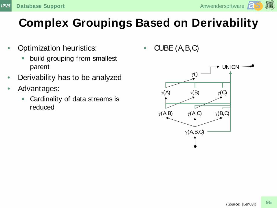
Complex Groupings Based on Derivability

• Optimization heuristics: build grouping from smallest

parent

• Derivability has to be analyzed • Advantages:

Cardinality of data streams is reduced

• CUBE (A,B,C)

γ(A,B,C)

γ()


γ(C) γ(B) γ(A)

UNION

(Source: [Len03])


ss

96

Exploiting Sort Order for Complex Groupings

• Optimization heuristics: use existing ordering e.g. sort data on A,B,C and

derive γ(A,B), γ(A), and γ() without additional sorts

• CUBE (A,B,C)

• Partial sort order may also be re-used

• Selection based on cardinality: |A|≥|B|≥|C|≥|D|

γ(A,B,C)

γ()


γ(C) γ(B) γ(A)

UNION

(Source: [Len03])

no additional sort

γ()

γ(A,C) γ(A,D) γ(A,B) γ(B,D) γ(C,D) γ(B,C)

γ(A,B,C) γ(A,B,D) γ(A,C,D) γ(B,C,D)

γ(A,B,C,D)

γ(C) γ(B) γ(A) γ(D)

keep partial sort order


ss

97

Algorithm for OLAP Functions

Begin SORT(G1, …, Gn, P1, …, Pm, O1, …, Op); While (Input not empty) $tuple = ReadNextTuple(Input); If (current and last tuple are equal for G1, …, Gn, P1, …, Pm) Then $aggrlist = $aggrlist + ($tuple); Else /* process partition */ For $pos = 1 To Length($aggrlist) Switch(WL) Case UNBOUNDED PRECEDING: $low = 1; Case CURRENT: $low = $pos; Default: $low = Max(1, $pos-WL); End Switch Switch (WH) Case UNBOUNDED FOLLOWING: $high = Length($aggrlist); Case CURRENT: $high = $pos; Default: $high = Min(Length($aggrlist), $pos+WH); End Switch $aggrval = AGG($aggrlist[$low], …, $aggrlist[$high]); WriteNextTuple(Output, G1, …, Gn, P1, …, Pm, O1, …, Op, $aggrval); End For $aggrlist = ($tuple); End If End While /* process last partiton similar to else path */ End

Gi: GROUP BY attributes Oj: WINDOW ordering (OVER clause) Pk: WINDOW partitioning WL, WH: lower and upper bound of WINDOW AGG: aggregation function

(Source: [Len03])


ss

98

Overview






ss

99

Key Criteria for Benchmarks

• Relevant: It must measure the peak performance and price/performance of systems.

• Portable: It should be easy to implement the benchmark on many different systems

and architectures.

• Scaleable: The benchmark should apply to small and large computer systems. It should

be possible to scale the benchmark up to larger systems, and to parallel computer systems as computer performance and architecture evolve.

• Simple: The benchmark must be understandable, otherwise it will lack credibility.

(J. Gray: The Benchmark Handbook for Database and Transaction Systems (2nd Edition), 1993)


ss

100

TPC-H

• Decision support benchmark. • Business oriented ad-hoc queries (Q1 - Q22) and concurrent data

modifications (RF1 - RF2). • Benchmark illustrates decision support systems that examine large

volumes of data, execute queries with a high degree of complexity, and give answers to critical business questions.

• Performance metric: TPC-H Composite Query-per-Hour Performance Metric (QphH@Size).

• TPC-H Price/Performance metric is expressed as $/QphH@Size.


ss

101

TPCH Benchmark Schema PARTSUPP (PS_)

SF*800.000 PARTKEY SUPPKEY AVAILQTY SUPPLYCOST COMMENT

ORDERS (O_) SF*1.500.000

ORDERKEY CUSTKEY ODERSTATUS TOTALPRICE ODERDATE ORDERPRIORITY CLERK SHIPPRIORITY COMMENT

LINEITEM (L_) SF*6.000.000

ORDERYEY PARTKEY SUPPKEY LINENUMBER QUANTITY EXTENDEDPRICE DISCOUNT TAX RETURNFLAG LINESTATUS SHIPDATE COMMITDATE RECEIPTDATE SHIPINSTRUCT SHIPMODE COMMENT

CUSTOMER (C_) SF*150.000

CUSTKEY NAME ADDRESS NATIONKEY PHONE ACCTBAL MKTSEGMENT COMMENT

PART (P_) SF*200.000

PARTKEY NAME MFGR BRAND TYPE SIZE CONTAINER RETAILPRICE COMMENT

NATION (N_) 25

NATIONKEY NAME REGIONKEY COMMENT

REGION (R_) 5

REGIONKEY NAME COMMENT

SUPPLIER (S_) SF*10.000

SUPPKEY NAME ADDRESS NATIONKEY PHONE ACCTBAL COMMENT

Database Scaling:

SF database size 1 1 GB 10 10 GB 30 30 GB 100 100 GB 300 300 GB 1000 1000 GB = 1 TB 3000 3000 GB 10000 10000 GB 30000 30000 GB 100000 100000 GB


ss

102

Minimum Cost Supplier Query (Q2)

• Business Question: The Minimum Cost Supplier Query finds, in a given region, for each part of a certain type and size, the supplier who can supply it at minimum cost. If several suppliers in that region offer the desired part type and size at the same (minimum) cost, the query lists the parts from suppliers with the 100 highest account balances. For each supplier, the query lists the supplier's account balance, name and nation; the part's number and manufacturer; the supplier's address, phone number and comment information.

SELECT s_acctbal, s_name, n_name, p_partkey, p_mfgr, s_address, s_phone, s_comment FROM part, supplier, partsupp, nation, region WHERE p_partkey = ps_partkey AND s_suppkey = ps_suppkey AND p_size = [SIZE] AND p_type like '%[TYPE]' AND s_nationkey = n_nationkey AND n_regionkey = r_regionkey AND r_name = '[REGION]' AND ps_supplycost = ( SELECT min(ps_supplycost) FROM partsupp, supplier, nation, region WHERE p_partkey = ps_partkey AND s_suppkey = ps_suppkey AND s_nationkey = n_nationkey AND n_regionkey = r_regionkey AND r_name = '[REGION]' ) ORDER BY s_acctbal desc, n_name, s_name, p_partkey;


ss

103

Refresh Functions

• Business Rationale (RF1): The New Sales refresh function inserts new rows into the ORDERS and LINEITEM tables in the database following the scaling and data generation methods used to populate the database.

• Refresh Function Definition: LOOP (SF * 1500) TIMES INSERT a new row into table ORDERS LOOP RANDOM(1, 7) TIMES INSERT a new row into LINEITEM END LOOP END LOOP

• Business Rationale (RF2): The Old Sales refresh function removes rows from the ORDERS and LINEITEM tables in the database to emulate the removal of stale or obsolete information.

• Refresh Function Definition: LOOP (SF * 1500) TIMES DELETE FROM ORDERS WHERE O_ORDERKEY = [value] DELETE FROM LINEITEM WHERE L_ORDERKEY = [value] END LOOP


ss

104

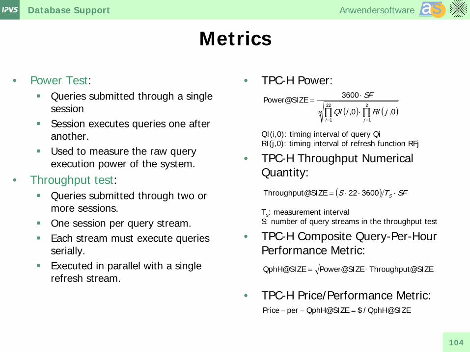
Metrics

• Power Test: Queries submitted through a single

session Session executes queries one after

another. Used to measure the raw query

execution power of the system.

• Throughput test: Queries submitted through two or

more sessions. One session per query stream. Each stream must execute queries

serially. Executed in parallel with a single

refresh stream.

• TPC-H Power: QI(i,0): timing interval of query Qi RI(j,0): timing interval of refresh function RFj

• TPC-H Throughput Numerical Quantity: Ts: measurement interval S: number of query streams in the throughput test

• TPC-H Composite Query-Per-Hour Performance Metric:

• TPC-H Price/Performance Metric:

( ) ( )24

2

1

22

10,0,

3600Power@SIZE

∏∏==

⋅

⋅=

jijRIiQI

SF

( ) SFTS S ⋅⋅⋅= 360022@SIZEThroughput

@SIZEThroughputPower@SIZEQphH@SIZE ⋅=

QphH@SIZE/$QphH@SIZEperPrice =−−


ss

105

TPC-H Results: 3 TB

(Source: www.tpc.org, October 2010)


ss

106

TPC-H Results: 10TB + 30TB

(Source: www.tpc.org, October 2010)


ss

107

TPC-R

• Decision support benchmark similar to TPC-H. • Allows additional optimizations based on advance knowledge

of the queries. • Business oriented queries and concurrent data modifications. • Performance metric: TPC-R Composite Query-per-Hour

Performance Metric (QphR@Size)- • TPC-R Price/Performance metric is expressed as $/QphR@Size.


ss

108

Summary

• SQL supports typical OLAP queries by: ROLLUP, CUBE, WINDOWs, Ranking, OLAP functions

• SQL/MM Data Mining supports: build data mining models (clustering, classification, regression, AR) test and apply data mining models import and export data mining models

• Database systems support performance of data warehouse systems by, e.g.: data partitioning materialized views indexes: bitmap indexes, join indexes, … query processing for star queries

• Benchmark for data warehousing: TPC-H


ss

109

Papers & Books

[Bay97] R. Bayer: The Universal B-Tree for Multidimensional Indexing: general Concepts In: Proc. of the Worldwide Computing and Its Applications, International Conference. WWCA '97, Tsukuba, Japan, March 10-11, 1997.

[BP+97] E. Baralis, S. Paraboschi, E. Teniente: Materialized View Selection in a Multidimensional Database. In: Proc. of the 23rd Int. Conf. on Very Large Databases, Athens, Greece, 1997.

[HR+96] V. Harinarayan, A. Rajaraman, J. Ullman: Implementing Data Cubes Efficiently. In: Proc. of the Int. Conf. on Management of Data, Montreal, Quebec, 1996.

[ScOu82] P. Scheuermann, M. Ouksel: Multidimensional B-trees for Associative Searching in Database Systems. In: Information Systems, vol. 7, no. 2, 1982.

[MS02] J. Melton, A. Simon: SQL:1999, Understanding Relational Language Components. Morgan Kaufmann, 2002.

[Mel03] J. Melton: SQL:1999, Understanding Object-Relational and other Advanced Features. Morgan Kaufmann, 2003.

data-warehouse-, data-mining- und olap … a anwendungssoftware s data-warehouse-, data-mining- und...

Documents