data warehousing overview. 2 warehousing l growing industry: $10 billion l range from desktop to...

Data Warehousing Overview

2

Warehousing

Growing industry: $10 billion Range from desktop to huge:

Walmart: 900-CPU, 2,700 disk, 23TBTeradata system

Lots of buzzwords, hype slice & dice, rollup, MOLAP, pivot, ...

3

Outline

What is a data warehouse? Why a warehouse? Models & operations Implementing a warehouse Future directions

4

What is a Warehouse?

Collection of diverse data subject oriented aimed at executive, decision maker often a copy of operational data with value-added data (e.g., summaries, history)

integrated time-varying non-volatile

more

5

What is a Warehouse?

Collection of tools gathering data cleansing, integrating, ... querying, reporting, analysis data mining monitoring, administering warehouse

6

Warehouse Architecture

Client Client

Warehouse

Source Source Source

Query & Analysis

Integration

Metadata

7

Motivating Examples

Forecasting Comparing performance of units Monitoring, detecting fraud Visualization

8

Why a Warehouse?

Two Approaches: Query-Driven (Lazy) Warehouse (Eager)

Source Source

?

9

Query-Driven Approach

Client Client

Wrapper Wrapper Wrapper

Mediator


10

Advantages of Warehousing

High query performance Queries not visible outside warehouse Local processing at sources unaffected Can operate when sources unavailable Can query data not stored in a DBMS Extra information at warehouse

Modify, summarize (store aggregates) Add historical information

11

Advantages of Query-Driven

No need to copy data less storage no need to purchase data

More up-to-date data Query needs can be unknown Only query interface needed at sources May be less draining on sources

12

OLTP vs. OLAP

OLTP: On Line Transaction Processing Describes processing at operational sites

OLAP: On Line Analytical Processing Describes processing at warehouse

13

OLTP vs. OLAP

Mostly updates Many small transactions Mb-Tb of data Raw data Clerical users Up-to-date data Consistency,

recoverability critical

Mostly reads Queries long, complex Gb-Tb of data Summarized,

consolidated data Decision-makers,

analysts as users

OLTP OLAP

14

Data Marts

Smaller warehouses Spans part of organization

e.g., marketing (customers, products, sales) Do not require enterprise-wide consensus

but long term integration problems?

15

Warehouse Models & Operators

Data Models relations stars & snowflakes cubes

Operators slice & dice roll-up, drill down pivoting other

16

Star

customer custId name address city53 joe 10 main sfo81 fred 12 main sfo

111 sally 80 willow la

product prodId name pricep1 bolt 10p2 nut 5

store storeId cityc1 nycc2 sfoc3 la

sale oderId date custId prodId storeId qty amto100 1/7/97 53 p1 c1 1 12o102 2/7/97 53 p2 c1 2 11105 3/8/97 111 p1 c3 5 50

17

Star Schema

saleorderId

datecustIdprodIdstoreId

qtyamt

customercustIdname

addresscity

productprodIdnameprice

storestoreId

city

18

Terms

Fact table Dimension tables Measures

saleorderId

datecustIdprodIdstoreId

qtyamt

customercustIdname

addresscity

productprodIdnameprice

storestoreId

city

19

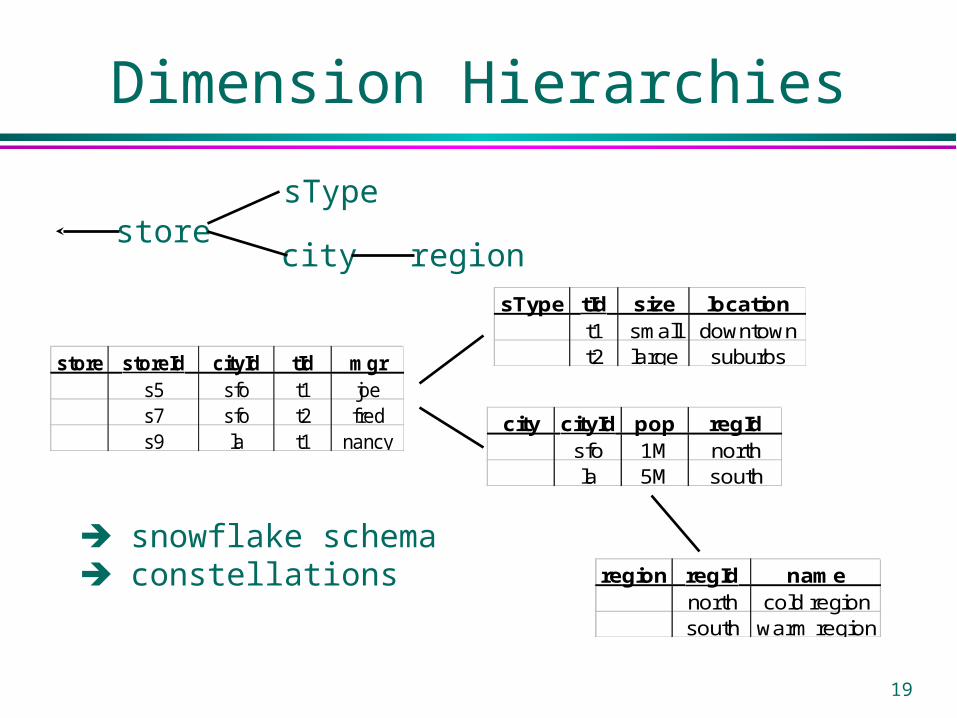
Dimension Hierarchies

store storeId cityId tId mgrs5 sfo t1 joes7 sfo t2 freds9 la t1 nancy

city cityId pop regIdsfo 1M northla 5M south

region regId namenorth cold regionsouth warm region

sType tId size locationt1 small downtownt2 large suburbs

storesType

city region

snowflake schema constellations

20

Cube

sale prodId storeId amtp1 c1 12p2 c1 11p1 c3 50p2 c2 8

c1 c2 c3p1 12 50p2 11 8

Fact table view: Multi-dimensional cube:

dimensions = 2

21

3-D Cube

sale prodId storeId date amtp1 c1 1 12p2 c1 1 11p1 c3 1 50p2 c2 1 8p1 c1 2 44p1 c2 2 4

day 2c1 c2 c3

p1 44 4p2 c1 c2 c3

p1 12 50p2 11 8

day 1

dimensions = 3

Multi-dimensional cube:Fact table view:

22

ROLAP vs. MOLAP

ROLAP:Relational On-Line Analytical Processing

MOLAP:Multi-Dimensional On-Line Analytical Processing

23

Aggregates


• Add up amounts for day 1• In SQL: SELECT sum(amt) FROM SALE WHERE date = 1

81

24

Aggregates


• Add up amounts by day• In SQL: SELECT date, sum(amt) FROM SALE GROUP BY date

ans date sum1 812 48

25

Another Example


• Add up amounts by day, product• In SQL: SELECT date, sum(amt) FROM SALE GROUP BY date, prodId

sale prodId date amtp1 1 62p2 1 19p1 2 48

drill-down

rollup

26

Aggregates

Operators: sum, count, max, min, median, ave

“Having” clause Using dimension hierarchy

average by region (within store) maximum by month (within date)

27

Cube Aggregation

day 2c1 c2 c3

p1 44 4p2 c1 c2 c3

p1 12 50p2 11 8

day 1

c1 c2 c3p1 56 4 50p2 11 8

c1 c2 c3sum 67 12 50

sump1 110p2 19

129

. . .

drill-down

rollup

Example: computing sums

28

Cube Operators

day 2c1 c2 c3

p1 44 4p2 c1 c2 c3

p1 12 50p2 11 8

day 1

c1 c2 c3p1 56 4 50p2 11 8

c1 c2 c3sum 67 12 50

sump1 110p2 19

129

. . .

sale(c1,*,*)

sale(*,*,*)sale(c2,p2,*)

29

c1 c2 c3 *p1 56 4 50 110p2 11 8 19* 67 12 50 129

Extended Cube

day 2 c1 c2 c3 *p1 44 4 48p2* 44 4 48

c1 c2 c3 *p1 12 50 62p2 11 8 19* 23 8 50 81

day 1

*

sale(*,p2,*)

30

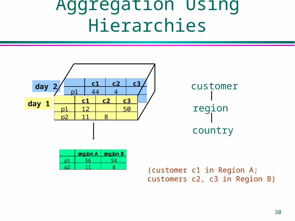
Aggregation Using Hierarchies

day 2c1 c2 c3

p1 44 4p2 c1 c2 c3

p1 12 50p2 11 8

day 1

region A region Bp1 56 54p2 11 8

customer

region

country

(customer c1 in Region A;customers c2, c3 in Region B)

31

Pivoting


day 2c1 c2 c3

p1 44 4p2 c1 c2 c3

p1 12 50p2 11 8

day 1

Multi-dimensional cube:Fact table view:

c1 c2 c3p1 56 4 50p2 11 8

32

Query & Analysis Tools

Query Building Report Writers (comparisons, growth, graphs,…)

Spreadsheet Systems Web Interfaces Data Mining

33

Other Operations

Time functions e.g., time average

Computed Attributes e.g., commission = sales * rate

Text Queries e.g., find documents with words X AND B e.g., rank documents by frequency of

words X, Y, Z

34

Data Mining

Decision Trees Clustering Association Rules

35

Decision Trees

sale custId car age city newCarc1 taurus 27 sf yesc2 van 35 la yesc3 van 40 sf yesc4 taurus 22 sf yesc5 merc 50 la noc6 taurus 25 la no

Example:• Conducted survey to see what customers were interested in new model car• Want to select customers for advertising campaign

trainingset

36

One Possibility


age<30

city=sf car=van

likely likelyunlikely unlikely

YY

Y

NN

N

37

Another Possibility


car=taurus

city=sf age<45

likely likelyunlikely unlikely

YY

Y

NN

N

38

Issues

Decision tree cannot be “too deep” would not have statistically significant amounts of

data for lower decisions

Need to select tree that most reliably predicts outcomes

39

Clustering

age

income

education

40

Another Example: Text

Each document is a vector e.g., <100110...> contains words 1,4,5,...

Clusters contain “similar” documents Useful for understanding, searching

documents

internationalnews

sports

business

41

Issues

Given desired number of clusters? Finding “best” clusters Are clusters semantically meaningful?

e.g., “yuppies’’ cluster? Using clusters for disk storage

42

Association Rule Mining

tran1 cust33 p2, p5, p8tran2 cust45 p5, p8, p11tran3 cust12 p1, p9tran4 cust40 p5, p8, p11tran5 cust12 p2, p9tran6 cust12 p9

transactio

n

id custo

mer

id products

bought

salesrecords:

• Trend: Products p5, p8 often bough together• Trend: Customer 12 likes product p9

market-basketdata

43

Association Rule

Rule: {p1, p3, p8} Support: number of baskets where these

products appear High-support set: support threshold s Problem: find all high support sets

44

Finding High-Support Pairs

Baskets(basket, item) SELECT I.item, J.item, COUNT(I.basket)

FROM Baskets I, Baskets JWHERE I.basket = J.basket AND I.item < J.itemGROUP BY I.item, J.itemHAVING COUNT(I.basket) >= s;

WHY?

45

Example

basket itemt1 p2t1 p5t1 p8t2 p5t2 p8t2 p11... ...

basket item1 item2t1 p2 p5t1 p2 p8t1 p5 p8t2 p5 p8t2 p5 p11t2 p8 p11... ... ...

check ifcount s

46

Issues

Performance for size 2 rulesbasket item

t1 p2t1 p5t1 p8t2 p5t2 p8t2 p11... ...

basket item1 item2t1 p2 p5t1 p2 p8t1 p5 p8t2 p5 p8t2 p5 p11t2 p8 p11... ... ...

bigevenbigger!

Performance for size k rules

47

Implementing a Warehouse

Monitoring: Sending data from sources Integrating: Loading, cleansing,... Processing: Query processing, indexing, ... Managing: Metadata, Design, ...

48

Monitoring

Source Types: relational, flat file, IMS, VSAM, IDMS, WWW, news-wire, …

Incremental vs. Refresh

customer id name address city53 joe 10 main sfo81 fred 12 main sfo

111 sally 80 willow la new

49

Monitoring Techniques

Periodic snapshots Database triggers Log shipping Data shipping (replication service) Transaction shipping Polling (queries to source) Screen scraping Application level monitoring

A

dvan

tage

s &

Dis

adva

ntag

es!!

50

Monitoring Issues

Frequency periodic: daily, weekly, … triggered: on “big” change, lots of changes, ...

Data transformation convert data to uniform format remove & add fields (e.g., add date to get history)

Standards (e.g., ODBC)

Gateways

51

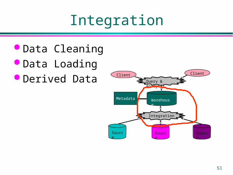
Integration

Data Cleaning Data Loading Derived Data

Client Client

Warehouse


Query & Analysis

Integration

Metadata

52

Data Cleaning

Migration (e.g., yen dollars) Scrubbing: use domain-specific knowledge (e.g.,

social security numbers) Fusion (e.g., mail list, customer merging)

Auditing: discover rules & relationships(like data mining)

billing DB

service DB

customer1(Joe)

customer2(Joe)

merged_customer(Joe)

53

Loading Data

Incremental vs. refresh Off-line vs. on-line Frequency of loading

At night, 1x a week/month, continuously Parallel/Partitioned load

54

Derived Data

Derived Warehouse Data indexes aggregates materialized views (next slide)

When to update derived data? Incremental vs. refresh

55

Materialized Views

Define new warehouse relations using SQL expressions


product id name pricep1 bolt 10p2 nut 5

joinTb prodId name price storeId date amtp1 bolt 10 c1 1 12p2 nut 5 c1 1 11p1 bolt 10 c3 1 50p2 nut 5 c2 1 8p1 bolt 10 c1 2 44p1 bolt 10 c2 2 4

does not existat any source

56

Processing

ROLAP servers vs. MOLAP servers Index Structures What to Materialize? Algorithms

Client Client

Warehouse


Query & Analysis

Integration

Metadata

57

ROLAP Server

Relational OLAP Server

relationalDBMS

ROLAPserver

tools

utilities

sale prodId date sump1 1 62p2 1 19p1 2 48

Special indices, tuning;

Schema is “denormalized”

58

MOLAP Server

Multi-Dimensional OLAP Server

multi-dimensional

server

M.D. tools

utilitiescould also

sit onrelational

DBMS

Pro

du

ctCity

Date1 2 3 4

milk

soda

eggs

soap

AB

Sales

59

Index Structures

Traditional Access Methods B-trees, hash tables, R-trees, grids, …

Popular in Warehouses inverted lists bit map indexes join indexes text indexes

60

Inverted Lists

2023

1819

202122

232526

r4r18r34r35

r5r19r37r40

rId name ager4 joe 20

r18 fred 20r19 sally 21r34 nancy 20r35 tom 20r36 pat 25r5 dave 21

r41 jeff 26

. .

.

ageindex

invertedlists

datarecords

61

Using Inverted Lists

Query: Get people with age = 20 and name = “fred”

List for age = 20: r4, r18, r34, r35 List for name = “fred”: r18, r52 Answer is intersection: r18

62

Bit Maps

2023

1819

202122

232526

id name age1 joe 202 fred 203 sally 214 nancy 205 tom 206 pat 257 dave 218 jeff 26

. .

.

ageindex

bitmaps

datarecords

110110000

0010001011

63

Using Bit Maps

Query: Get people with age = 20 and name = “fred”

List for age = 20: 1101100000 List for name = “fred”: 0100000001 Answer is intersection: 010000000000

Good if domain cardinality small Bit vectors can be compressed

64

Join


• “Combine” SALE, PRODUCT relations• In SQL: SELECT * FROM SALE, PRODUCT

product id name pricep1 bolt 10p2 nut 5

joinTb prodId name price storeId date amtp1 bolt 10 c1 1 12p2 nut 5 c1 1 11p1 bolt 10 c3 1 50p2 nut 5 c2 1 8p1 bolt 10 c1 2 44p1 bolt 10 c2 2 4

65

Join Indexes

product id name price jIndexp1 bolt 10 r1,r3,r5,r6p2 nut 5 r2,r4

sale rId prodId storeId date amtr1 p1 c1 1 12r2 p2 c1 1 11r3 p1 c3 1 50r4 p2 c2 1 8r5 p1 c1 2 44r6 p1 c2 2 4

join index

66

What to Materialize?

Store in warehouse results useful for common queries

Example:day 2

c1 c2 c3p1 44 4p2 c1 c2 c3

p1 12 50p2 11 8

day 1

c1 c2 c3p1 56 4 50p2 11 8

c1 c2 c3p1 67 12 50

c1p1 110p2 19

129

. . .

total sales

materialize

67

Materialization Factors

Type/frequency of queries Query response time Storage cost Update cost

68

Cube Aggregates Lattice

city, product, date

city, product city, date product, date

city product date

all

day 2c1 c2 c3

p1 44 4p2 c1 c2 c3

p1 12 50p2 11 8

day 1

c1 c2 c3p1 56 4 50p2 11 8

c1 c2 c3p1 67 12 50

129

use greedyalgorithm todecide whatto materialize

69


all

state

city

cities city statec1 CAc2 NY

70


city, product

city, product, date

city, date product, date

city product date

all

state, product, date

state, date

state, product

state

not all arcs shown...

71

Interesting Hierarchy

all

years

quarters

months

days

weeks

time day week month quarter year1 1 1 1 20002 1 1 1 20003 1 1 1 20004 1 1 1 20005 1 1 1 20006 1 1 1 20007 1 1 1 20008 2 1 1 2000

conceptualdimension table

72

Algorithms

Query Optimization Parallel Processing Data Mining

73

Example: Association Rules

How do we perform rule mining efficiently? Observation: If set X has support t, then

each X subset must have at least support t For 2-sets:

if we need support s for {i, j} then each i, j must appear in at least s

baskets

74

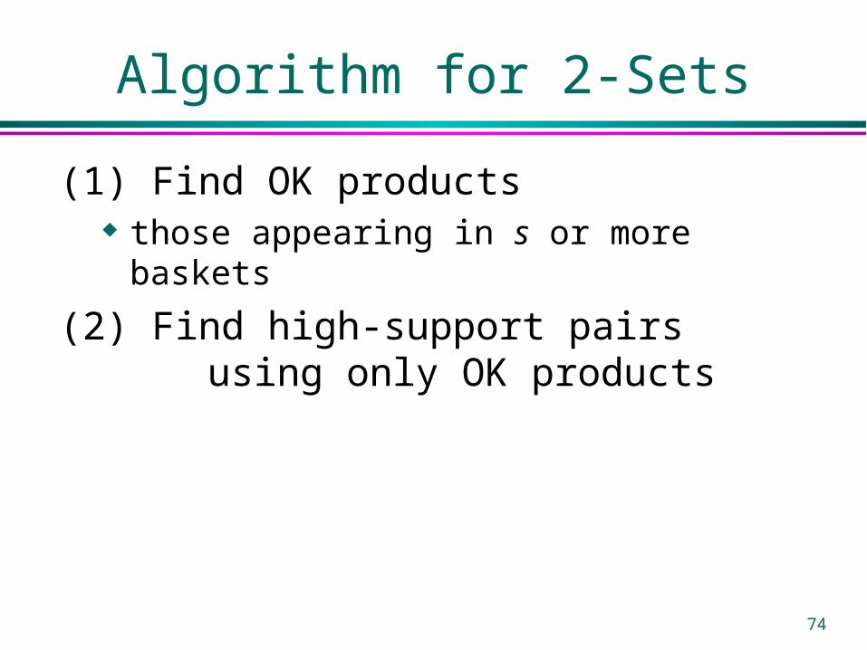
Algorithm for 2-Sets

(1) Find OK products those appearing in s or more baskets

(2) Find high-support pairs using only OK products

75

Algorithm for 2-Sets

INSERT INTO okBaskets(basket, item) SELECT basket, item FROM Baskets GROUP BY item HAVING COUNT(basket) >= s;

Perform mining on okBaskets SELECT I.item, J.item, COUNT(I.basket) FROM okBaskets I, okBaskets J WHERE I.basket = J.basket AND I.item < J.item GROUP BY I.item, J.item HAVING COUNT(I.basket) >= s;

76

Counting Efficiently

One way:

basket I.item J.itemt1 p5 p8t2 p5 p8t2 p8 p11t3 p2 p3t3 p5 p8t3 p2 p8... ... ...

sort


count &remove count I.item J.item

3 p5 p85 p12 p18... ... ...

threshold = 3

77

Counting Efficiently

Another way:


remove count I.item J.item3 p5 p85 p12 p18... ... ...

scan &count

count I.item J.item1 p2 p32 p2 p83 p5 p85 p12 p181 p21 p222 p21 p23... ... ...

keep counterarray in memory

threshold = 3

78

Yet Another Way


(1)scan &hash &count

count bucket1 A5 B2 C1 D8 E1 F... ...

in-memoryhash table threshold = 3


(2) scan &remove

count I.item J.item3 p5 p85 p12 p18... ... ...

(4) removecount I.item J.item

3 p5 p81 p8 p115 p12 p18... ... ...

(3) scan& count

in-memorycounters

false positive

79

Discussion

Hashing scheme: 2 (or 3) scans of data Sorting scheme: requires a sort! Hashing works well if few high-support pairs

and many low-support ones

item-pairs ranked by frequency

fre

que

ncy

threshold

iceberg queries

80

Managing

Metadata Warehouse Design Tools

Client Client

Warehouse


Query & Analysis

Integration

Metadata

81

Metadata

Administrative definition of sources, tools, ... schemas, dimension hierarchies, … rules for extraction, cleaning, … refresh, purging policies user profiles, access control, ...

82

Metadata

Business business terms & definition data ownership, charging

Operational data lineage data currency (e.g., active, archived, purged) use stats, error reports, audit trails

83

Design

What data is needed? Where does it come from? How to clean data? How to represent in warehouse (schema)? What to summarize? What to materialize? What to index?

84

Tools

Development design & edit: schemas, views, scripts, rules, queries, reports

Planning & Analysis what-if scenarios (schema changes, refresh rates), capacity planning

Warehouse Management performance monitoring, usage patterns, exception reporting

System & Network Management measure traffic (sources, warehouse, clients)

Workflow Management “reliable scripts” for cleaning & analyzing data

85

Current State of Industry

Extraction and integration done off-line Usually in large, time-consuming, batches

Everything copied at warehouse Not selective about what is stored Query benefit vs storage & update cost

Query optimization aimed at OLTP High throughput instead of fast response Process whole query before displaying

anything

86

Future Directions

Better performance Larger warehouses Easier to use What are companies & research labs

working on?

87

Research (1)

Incremental Maintenance Data Consistency Data Expiration Recovery Data Quality Error Handling (Back Flush)

88

Research (2)

Rapid Monitor Construction Temporal Warehouses Materialization & Index Selection Data Fusion Data Mining Integration of Text & Relational Data

89

Conclusions

Massive amounts of data and complexity of queries will push limits of current warehouses

Need better systems: easier to use provide quality information

data warehousing overview. 2 warehousing l growing industry: $10 billion l range from desktop to...

Documents