Raman spectroscopy in open world learning settings using the

Objectosphere approach

Yaroslav Balytskyi,1, 2, ∗ Justin Bendesky,2, 3

Tristan Paul,1, 2 Guy Hagen,2 and Kelly McNear1, 2

1Department of Physics and Energy Science,

University of Colorado Colorado Springs,

Colorado Springs, CO, 80918, USA

2UCCS BioFrontiers Center, University of Colorado Colorado Springs,

Colorado Springs, CO, 80918, USA

3Department of Chemistry, New York University, New York, NY 10003, USA

(Dated: November 12, 2021)

1

arX

iv:2

111.

0626

8v1

[cs

.LG

] 1

1 N

ov 2

021

Abstract

Raman spectroscopy in combination with machine learning has significant promise for applica-

tions in clinical settings as a rapid, sensitive, and label-free identification method. These approaches

perform well in classifying data that contains classes that occur during the training phase. How-

ever, in practice, there are always substances whose spectra have not yet been taken or are not

yet known and when the input data are far from the training set and include new classes that

were not seen at the training stage, a significant number of false positives are recorded which

limits the clinical relevance of these algorithms. Here we show that these obstacles can be over-

come by implementing recently introduced Entropic Open Set and Objectosphere loss functions.

To demonstrate the efficiency of this approach, we compiled a database of Raman spectra of 40

chemical classes separating them into 20 biologically relevant classes comprised of amino acids, 10

irrelevant classes comprised of bio-related chemicals, and 10 classes that the Neural Network has

not seen before, comprised of a variety of other chemicals. We show that this approach enables the

network to effectively identify the unknown classes while preserving high accuracy on the known

ones, dramatically reducing the number of false positives while preserving high accuracy on the

known classes, which will allow this technique to bridge the gap between laboratory experiments

and clinical applications.

Keywords: Raman spectroscopy; Machine learning; ResNet; Open set learning; Objectosphere; Clinical

applications.

∗Electronic address: ybalytsk@uccs.edu

2

Introduction

Bacterial infections are responsible for severe diseases and cause 7 million deaths annu-

ally [1, 2]. The conventional methods for bacteria detection in clinical applications, enzyme-

linked immunosorbent assays (ELISA), and strategies based on the polymerase chain re-

action (PCR) and sequencing take significant time [3–6]. Clinical diagnostic results are

often delayed up to 48 hours for microbiological culture with an additional 24 hours for

antibiotic susceptibility testing. While waiting for the results, broad-spectrum antibiotics

(BSAbx) are typically applied until a specific pathogen is identified. Even though BSAbx

are often lifesaving, they contribute to the rise of antibiotic resistant strains of bacteria and

decimate the healthy gut microbiome, leading to overgrowth of pathogens such as Candida

albicans and Clostridium difficile [7, 8], and according to the Centers for Disease Control

and Prevention, over 30% of patients are treated unnecessarily [9]. As a result, delays in

pathogen identification ultimately lead to longer hospital stays, higher medical costs, and

increased antibiotic resistance and mortality [10]. There is a clear need for new culture-free,

rapid, cost-effective and highly sensitive detection and identification methods to ensure that

targeted antibiotics are applied as a means to mitigate antimicrobial resistance.

Raman spectroscopy is a non-destructive technique that has the ability to meet these

requirements by providing a unique, fingerprint-like spectrum of a sample. It consists of

inelastic light scattering from a sample and the successive measurement of the energy shift

of scattered photons by the detector [11]. While Raman spectroscopy is a highly sensitive

technique capable of identifying a wide variety of chemical species, analyzing the spectra can

be difficult and data processing is necessary to identify species with the accuracy needed for

clinical applications. Due to the large amounts of data which is acquired, it is difficult and

impractical to hard-code all rules of classification. Automating this process requires some

form of Machine Learning (ML) which represents a code being capable of improving itself

by learning the relevant features from the data rather than hard-coding them. After the

new knowledge is acquired, it can be used to tackle real-world problems such as performing

classification or regression [12].

Machine learning has proven itself to be a powerful tool in multiple applications. For ex-

ample, shallow ML models, such as logistic regression, can be employed in some situations,

but in order for such shallow models to work, one has to choose the relevant features manu-

3

ally, i.e. perform feature engineering to enable the classification operation. In other words,

the relevant features have to be fed into the model manually. To overcome this limitation,

deep learning (DL) models using neural networks (NN) have been developed, allowing mod-

els to explore very abstract features with little human intervention. Deep learning models

with various architectures were applied with great success in image processing [13–16] as

well as speech [17, 18] recognition. Not only this, but DL methods can be applied to a vari-

ety of fields; from medicine [19–21] and food safety [22] to particle physics [23]. It was later

found that DL methods can effectively distinguish the spectra of different molecules [24]

and do so more effectively than linear regression methods for data analysis in Raman spec-

troscopy [25]. This demonstrates that these methods are ideal to explore for our goals. DL

methods using convolutional neural networks were shown to boost the accuracy in compar-

ison with other types of dense networks [26], which can suffer from a vanishing gradient

problem, preventing increases in accuracy [27]. The ResNet architecture overcomes this

problem and boosts the accuracy even further by introducing skip connections between the

layers [28]. Current state-of-the art deep learning algorithms for Raman spectroscopy favor

the ResNet architecture because it can maintain high performance at a lower complexity

than its competitors. Using these advances, Raman spectroscopy combined with machine

learning has shown significant promise for clinical use as a rapid, label-free identification

method [29–34].

However, a significant limitation of the aforementioned NNs are that they are only tested

on the classes on which they were initially trained. As a result, if the inputs for the NN

are far from the training set and include new, never seen before classes, the NN’s behavior

becomes ill-defined. Simply put, if the NN is trained to identify either “cats” or “dogs”

but during testing sees a new class of “fish”, the false-positive rate becomes uncontrolled

and the NN will misclassify “fish” as either “cat” or “dog”. When we consider real-world

settings and practical applications, collecting data of all possible chemical or pathogenic

species is not feasible, so there will always be unknown classes. To avoid false-positives

and misclassification, the ideal NN should be able to not only classify the known samples,

but also be able to handle any unknowns without misclassification. This obstacle is a

significant limitation in the currently deployed ML systems and represents a gap between

the developments of novel identification methods and their adoption into routine clinical

practices.

4

To overcome this obstacle, we implement ideas from Entropic Open-Set and Objecto-

sphere approaches [35] and combine them with the ResNet26 architecture to show, for the

first time, that ResNet architecture can be modified to accurately and reliably reject sam-

ples it has not seen before while remaining highly accurate in its identification of the known

classes. This new combined architecture significantly outperforms the naive approaches such

as the thresholding softmax score [36–38] and background class methods [36]. The general

idea of implementing these approaches is to teach the NN to ignore the features of the ir-

relevant classes and only focus on the features of the relevant classes. To demonstrate the

efficiency of our approach, we compiled a database of spectra of 40 chemical classes and sep-

arated them into distinct categories. Twenty of them are amino acids, the building blocks of

proteins. The remaining 20 classes were split into two groups of 10 for the purpose of testing

the classification accuracy of the NN. The spectra of the 20 amino acids were categorized

as “known”, and the remaining 20 chemicals were randomly split into two groups we called

“ignored” or “never seen before”. The samples from the “never seen before” class are unique

in that the NN was not trained on them and does not see them until the testing stage. For

our purposes, we introduced the following conventions of “known classes”, “ignored classes”

and “never seen classes”:K − known classes or classes of interest

I − ignored classes

N − never seen before classes

During the training stage, the NN is taught to be highly accurate on the K classes and

separate them from the I classes. During the test stage, we test its accuracy on K as well

as determine the rate number of false positives of N .

Data collection and ResNet26 architecture

The 20 simple amino acids were purchased from Carolina Biological Supply Company

(Burlington, NC). All other chemicals were purchased from either Alfa Aesar or Sigma

Aldrich. All samples were measured in their crystalline form on a glass-bottomed petri dish.

Raman maps were collected on a WITec alpha300 microscope in the confocal Raman mode,

schematically shown in Fig. 1. The excitation source was a 75 mW, 532 nm laser, focused

5

with a Zeiss EC-Epiplan 20x 0.4 NA objective. A WITec UHTS 300 spectrometer with a 600

groove/mm grating was used to collect the spectra. The detector was an Andor DV401-BV

spectroscopic CCD. This spectrometer has a resolution of 3 cm-1 or 0.009 nm. Raman maps

were collected over an area of 50 µm by 50 µm. This area was divided into 100 x 100 pixels,

each containing a Raman spectrum collected with an integration time of 0.1 seconds. Of

the collected spectra, 56

were used for training and 16

were used for testing. Before feeding

the data into the NN, the spectra are normalized, as shown in Fig. 2. To do this, the large

Rayleigh peak from the laser is cut and the subsequent spectrum is rescaled into a [0, 1]

range.

Figure 1: Schematic drawing of our experimental setup. The incident 532 nm green laser interacts

with the sample on a glass slide and the scattered light (red) is collected by the dectector.

6

Figure 2: Representative spectra for (a) raw and (b) normalized lysine data

Once the spectra were collected, they were categorized as either “known”, “ignored”, or

“never seen” and are detailed in Table I.

Class Chemical Name

K

DL-alanine, DL-aspartic acid, DL-isoleucine, DL-leucine,DL-methionine,

DL-phenylalanine, DL-serine, DL-threonine, DL-tyrosine, DL-valine,

glycine, L-arginine, L-asparagine, L-cystine, L-glutamic acid, L-histidine,

L-lysine, L(+)-cysteine, L-proline, L-tryptophan

Ianthrone, beta estradiol, chloroquine, fluconazole, laminarin, lauric acid,

MOPS, methyl viologen, progesterone, uridine

N

ampicillin, CHAPS, D(+) maltose monohydrate, forskolin,

1-Decanesulfonic acid, polyvinyl pyrrolidone, potato starch,

sodium deoxycholate, sodium dodecylsulfate, silver nitrate

Table I: Table of chemical names for known (K), ignored (I), and never seen before (N ) class

identifications.

First, to make sure that our NN has sufficiently high accuracy in the “closed-world”

settings, we expose it to all classes, K, I and N . The conventional ResNet26 architecture

shown in Fig. 3 is run 5 times as a means to help boost the accuracy of the network. While

a few misclassifications may occur during each separate run, we can average the predictions

(e.g. majority voting), and boost the accuracy to 99.99% as shown in Fig. 4. The accuracies

7

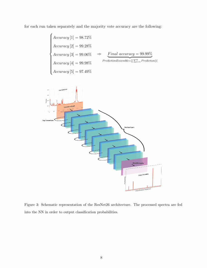
for each run taken separately and the majority vote accuracy are the following:

Accuracy [1] = 98.72%

Accuracy [2] = 99.28%

Accuracy [3] = 99.06%

Accuracy [4] = 99.98%

Accuracy [5] = 97.49%

⇒ Final accuracy = 99.99%︸ ︷︷ ︸PredictionEnsemble= 1

5

∑5i=1 Prediction[i]

Figure 3: Schematic representation of the ResNet26 architecture. The processed spectra are fed

into the NN in order to output classification probabilities.

8

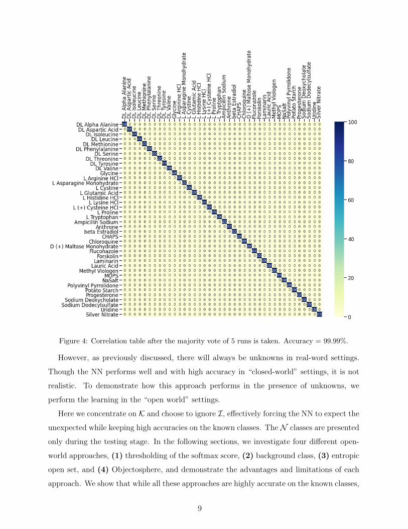
Figure 4: Correlation table after the majority vote of 5 runs is taken. Accuracy = 99.99%.

However, as previously discussed, there will always be unknowns in real-word settings.

Though the NN performs well and with high accuracy in “closed-world” settings, it is not

realistic. To demonstrate how this approach performs in the presence of unknowns, we

perform the learning in the “open world” settings.

Here we concentrate on K and choose to ignore I, effectively forcing the NN to expect the

unexpected while keeping high accuracies on the known classes. The N classes are presented

only during the testing stage. In the following sections, we investigate four different open-

world approaches, (1) thresholding of the softmax score, (2) background class, (3) entropic

open set, and (4) Objectosphere, and demonstrate the advantages and limitations of each

approach. We show that while all these approaches are highly accurate on the known classes,

9

having Accuracy = 99.97 ± 0.02%, the Objectosphere approach is much more efficient in

treating the N classes and is better prepared for unexpected inputs.

Background Class and Thresholding the Softmax Score

First, we review the necessary background and terminology associated with neural net-

works. The NN has an initial input, x, which in our case corresponds to the values of the

intensities in the spectra. The output corresponding to each class is lc (x). The deep feature

of the NN, F , is the output of the layer of the NN before the last one, and the output is

obtained by multiplication by the weights W to the last layer:

lc(x) = W · F (x)

The final probability of which class, c, that a particular input will belong to is calculated

by the “softmaxing” procedure:

Sc (x) =elc(x)∑c e

lc(x)

which lies in the range Sc (x) ∈ [0; 1], and∑

c Sc (x) = 1 and therefore is interpreted as a

probability. The input sample will be classified as whichever class has the highest output

probability.

The output of the NN is high-dimensional, so to provide a reasonable visualization, we

use the Uniform Manifold Approximation and Projection (UMAP) dimensionality reduction

technique [39]. This allows for the high-dimensional output of the NN to be visualized in

a 2-dimensional way. In all our runs, we used the default parameters of the algorithm. In

a 2D plane, different classes correspond to different colors, and should be separated from

each other if the NN is highly accurate. In the case that there is any overlap of points of

different colors, this indicates a mistake of the NN. As an example, in the “closed-world”

settings with 40 classes, the UMAP output is provided in Fig. 5. Each class of the 40 classes

correspond to a color in the gradient shown and we observe good separation between them

and note that each color is concentrated in a particular point of a 2D space rather than

being scattered over all the plane, a good indication that the NN is classifying efficiently.

As we shift to the “open-world” learning setting, the K classes correspond to the red to

blue gradient. When new, never seen before classes are present during the testing stage, we

group these unknowns together and represent them as violet dots on the UMAP diagrams.

10

Figure 5: UMAP of 40 classes in the closed world setting.

When the unknown, never seen before classes are present, one naive approach is to include

a trash or background class which corresponds to the background class method. The amino

acid number i ∈ [0, C − 1], and the {I,N} classes are encoded as:

(Amino acid) [i] =

0, · · · , 1︸︷︷︸ith position

, · · · , 0

︸ ︷︷ ︸

Length=C+1

; N =

0, · · · , 1︸︷︷︸20th position

︸ ︷︷ ︸

Length=C+1

,

where C = 20 - number of classes of interest (amino acids).

Another naive approach is to threshold the softmax score, which assumes that the K and

{I,N} classes are sufficiently separated in the feature space. In other words, Shannon’s

entropy of NN’s output on the {I,N} classes is close to the maximal value log2 (C):

{I,N} =

[1

C, · · · , 1

C

]︸ ︷︷ ︸

Length=C

while the entropy of the output of K classes is close to zero. Assuming that this condition is

fulfilled, one can introduce a cutoff, and if the maximum value of the softmax score is lower

than its value, the input is classified as the new, never seen before class.

11

However, as can be seen in Fig. 6, both the background class and thresholding the softmax

score methods—despite having a high accuracy on the known classes—work poorly if the

N classes are present and significantly mixes the knowns and unknowns. As illustrated in

Fig. 7, even in a case of introducing a high cutoff value of Λ = 0.99 (corresponding to the

NN being confident by 99%), the false positive (FP ) rate is 10.0%. Additionally, on the K

classes, in 7.0% of the cases the NN produces an inconclusive output, i.e. classifies K to be

belonging to the N classes.

Figure 6: UMAP diagrams of (a) the background class and (b) the thresholding the softmax score

methods. Class N (violet) is scattered over a large part of the diagram, mixing the known and the

unknown.

12

Figure 7: Even at the large cutoff value Λ = 0.99, the FP = 10.0%, and the number of inconclusive

outcomes on K classes is 7.0%.

Though the absolute values of the deep features ||F || of the known tends to be slightly

higher than those of ignored and unknowns as shown in Fig. 8, the amount of overlap between

the three classes indicates that the NN has difficulty distinguishing between K and N . The

Entropic Open Set and Objectosphere approaches aim to increase this separation.

Figure 8: The absolute value of the deep feature ||F || of K classes tends to be higher than those

of N and I.

13

Entropic Open Set and Objectosphere methods

The Entropic Open Set loss function [35] is defined as:

VE (x) =

− log (Sc (x)) , if x ∈ K

− 1C

∑Cc=1 log (Sc (x)) , if x ∈ I

where C = 20 is the number of classes of interest (amino acids). Note, for the K classes,

it reduces to a regular categorical cross entropy loss function, and the N classes are not

involved, since the NN is not aware of them until the testing stage. For the samples belonging

to I classes, VE (x) aims to maximize the entropy, and uniformly spread the NN’s output

over the known classes K.

The Objectosphere loss function involves the addition of the deep feature F , and mini-

mizes its absolute value for the ignored classes and maximizes it for the known ones:

VO (x) = VE (x) + α

max (β − ||F ||2, 0) , if x ∈ K

||F ||2, if x ∈ I

effectively increasing the separation between the K and {I,N} classes. The values of α and

β are adjusted numerically by minimizing the number of inconclusive outcomes on the K

classes. The result of this that FP = 0% on the I classes.

Both these approaches provide a significant improvement over the naive approaches as

shown in Fig. 9. For the entropic open set loss function shown in Fig. 9(a), at the cutoff

value ΛEntropic = 0.93, FP = 0%, the NN has 0% wrong outcomes on the known classes,

and number of inconclusive outcomes on the known classes is 2.37%. For the Objectosphere

loss function shown in Fig. 9(b), at the cutoff value ΛObjectosphere = 0.91, FP = 0%, 0%

wrong outcomes on the known classes, and the number of inconclusive outcomes on the

known classes is drastically reduced to 0.26% as shown in Fig. 9. This shows that the

Objectosphere reduces inconclusive outcomes by 89% from the entropic open set loss and

96% from the naive approaches, which is a significant improvement and demonstrates that

the Objectosphere approach successfully avoids misclassifications and false positives.

The corresponding UMAPs shown in Fig. 10 demonstrate a significant improvement in

treating the N classes by the NN. The area taken by the N classes is significantly reduced

14

in comparison with the previous approaches, one can make a clear distinction between N

and K classes and draw a line separating them.

Figure 9: Results of the (a) Entropic Open Set and (b) Objectosphere loss functions. The Objecto-

sphere improves the treatment of the N classes even more by reducing the number of inconclusive

outcomes on the K classes to 0.26%.

Figure 10: UMAPs for the (a) Entropic Open Set and (b) Objectosphere loss functions. For the

Objectosphere case, the area over which the N classes are scattered shrinks significantly and a

clear separation between K and N is observed.

Finally, as one can observe in Fig. 11, the Objectosphere loss function enhances the

separation between the features of the N and K classes minimizing the incorrect responses

from the NN to the new, never seen before inputs.

15

Figure 11: Distribution of the deep features of the known (K) and unknown/unexpected inputs

(N ) by the (a) Entropic Open Set and (b) Objectosphere loss functions. An improved separation

of K/N classes for the case of Objectosphere is observed.

Conclusions and future work

Raman spectroscopy in combination with Machine Learning demonstrates significant

promise as a fast, label-free, pathogen identification method. It has the potential to reduce

treatment costs, mitigate antibiotic resistance, and save human lives. However, traditional

ML architectures applied in this context only work in closed-world settings and become

ill-defined when presented with unknowns, limiting their practical applications. Here we

have shown that we can overcome this challenge by modifying ResNet26 architecture. The

application of the recently introduced entropic open set and Objectosphere approaches en-

ables the ResNet26 architecture to maintain a high accuracy on the known classes while

successfully avoiding misclassification of new, never seen before classes. This method is

an important step towards the translation of using machine learning methods in clinical

applications. In future work we plan to explore mixtures of chemical classes and spectra

with low signal-to-noise ratios to better mimic real-world settings and further improve the

performance of our neural network.

16

Code availability and reproducibility of our results

1Our code is publicly available on GitHub. In order to reproduce our results, one needs

to upload this data and code into Google Colab [40], connect to the TPU, and follow the

instructions in the Jupyter notebooks provided.

Acknowledgments

Research reported in this publication was supported by the National Institute of General

Medical Sciences of the National Institutes of Health under award No. 1R15GM128166–01.

This work was also supported by the UCCS BioFrontiers Center. The funding sources had

no involvement in study design; in the collection, analysis, and interpretation of data; in

the writing of the report; or in the decision to submit the article for publication. This work

was supported in part by the U.S. Civilian Research & Development Foundation (CRDF

Global). The authors would like to thank Kyle Culhane, Van Hovenga, and Anatoliy Pinchuk

for useful discussions.

Author Contributions

All authors discussed the organization and content of the manuscript. YB developed the

modification to the ResNet26 architecture, helped to collect Raman maps of the chemical

classes, and wrote the main manuscript. JB and TP helped to collect the Raman maps of

the 40 chemical classes. GH supervised the work, assisted in the experimental design and

revised the manuscript. KM supervised the work, critically reviewed, and revised the main

manuscript.

Ethics Declaration

The authors declare no competing interests.

1 https://github.com/BalytskyiJaroslaw/RamanOpenSet.git

17

[1] Carolin Fleischmann, Andre Scherag, Neill KJ Adhikari, Christiane S Hartog, Thomas

Tsaganos, Peter Schlattmann, Derek C Angus, and Konrad Reinhart. Assessment of global

incidence and mortality of hospital-treated sepsis. current estimates and limitations. American

Journal of Respiratory and Critical Care Medicine, 193(3):259–272, 2016.

[2] Rodrigo DeAntonio, Juan-Pablo Yarzabal, James Philip Cruz, Johannes E Schmidt, and Jos

Kleijnen. Epidemiology of community-acquired pneumonia and implications for vaccination

of children living in developing and newly industrialized countries: A systematic literature

review. Human Vaccines & Immunotherapeutics, 12(9):2422–2440, 2016.

[3] Philip D Howes, Subinoy Rana, and Molly M Stevens. Plasmonic nanomaterials for biodiag-

nostics. Chemical Society Reviews, 43(11):3835–3853, 2014.

[4] Hyun Jung Chung, Cesar M Castro, Hyungsoon Im, Hakho Lee, and Ralph Weissleder. A

magneto-DNA nanoparticle system for rapid detection and phenotyping of bacteria. Nature

Nanotechnology, 8(5):369–375, 2013.

[5] Mitchell M Levy, Laura E Evans, and Andrew Rhodes. The surviving sepsis campaign bundle:

2018 update. Intensive Care Medicine, 44(6):925–928, 2018.

[6] A Chaudhuri, PM Martin, PGE Kennedy, R Andrew Seaton, P Portegies, M Bojar, I Steiner,

and EFNS Task Force. Efns guideline on the management of community-acquired bacterial

meningitis: report of an efns task force on acute bacterial meningitis in older children and

adults. European Journal of Neurology, 15(7):649–659, 2008.

[7] Nele Brusselaers, Dirk Vogelaers, and Stijn Blot. The rising problem of antimicrobial resistance

in the intensive care unit. Annals of Intensive Care, 1(1):1–7, 2011.

[8] Asa Sullivan, Charlotta Edlund, and Carl Erik Nord. Effect of antimicrobial agents on the

ecological balance of human microflora. The Lancet Infectious Diseases, 1(2):101–114, 2001.

[9] Katherine E Fleming-Dutra, Adam L Hersh, Daniel J Shapiro, Monina Bartoces, Eva A Enns,

Thomas M File, Jonathan A Finkelstein, Jeffrey S Gerber, David Y Hyun, Jeffrey A Linder,

et al. Prevalence of inappropriate antibiotic prescriptions among us ambulatory care visits,

2010-2011. JAMA, 315(17):1864–1873, 2016.

[10] Julian Davies and Dorothy Davies. Origins and evolution of antibiotic resistance. Microbiology

and Molecular Biology Reviews, 74(3):417–433, 2010.

18

[11] Shintaro Pang, Tianxi Yang, and Lili He. Review of surface enhanced raman spectroscopic

(sers) detection of synthetic chemical pesticides. TrAC Trends in Analytical Chemistry, 85:73–

82, 2016.

[12] Ian Goodfellow, Yoshua Bengio, and Aaron Courville. Deep learning. MIT press, 2016.

[13] Alex Krizhevsky, Ilya Sutskever, and Geoffrey E Hinton. Imagenet classification with deep

convolutional neural networks. Advances in Neural Information Processing Systems, 25:1097–

1105, 2012.

[14] Clement Farabet, Camille Couprie, Laurent Najman, and Yann LeCun. Learning hierarchical

features for scene labeling. IEEE Transactions on Pattern Analysis and Machine Intelligence,

35(8):1915–1929, 2012.

[15] Christian Szegedy, Wei Liu, Yangqing Jia, Pierre Sermanet, Scott Reed, Dragomir Anguelov,

Dumitru Erhan, Vincent Vanhoucke, and Andrew Rabinovich. Going deeper with convolu-

tions. In Proceedings of the IEEE conference on Computer Vision and Pattern Recognition,

pages 1–9, 2015.

[16] Guy M. Hagen, Justin Bendesky, Rosa Machado, Tram-Ahn Nguyen, Ranman Kumar, and

Jonathan Ventura. Fluorescence microscopy datasets for training deep neural networks. Gi-

gascience, 10(5):giab032, 2021.

[17] George E Dahl, Tara N Sainath, and Geoffrey E Hinton. Improving deep neural networks

for lvcsr using rectified linear units and dropout. In 2013 IEEE International Conference on

Acoustics, Speech and Signal Processing, pages 8609–8613. IEEE, 2013.

[18] Geoffrey Hinton, Li Deng, Dong Yu, George E Dahl, Abdel-Rahman Mohamed, Navdeep

Jaitly, Andrew Senior, Vincent Vanhoucke, Patrick Nguyen, Tara N Sainath, et al. Deep

neural networks for acoustic modeling in speech recognition: The shared views of four research

groups. IEEE Signal Processing Magazine, 29(6):82–97, 2012.

[19] Royston Goodacre, Eadaoin M Timmins, Rebecca Burton, Naheed Kaderbhai, Andrew M

Woodward, Douglas B Kell, and Paul J Rooney. Rapid identification of urinary tract infec-

tion bacteria using hyperspectral whole-organism fingerprinting and artificial neural networks.

Microbiology, 144(5):1157–1170, 1998.

[20] Sigurdur Sigurdsson, Peter Alshede Philipsen, Lars Kai Hansen, Jan Larsen, Monika Gni-

adecka, and Hans-Christian Wulf. Detection of skin cancer by classification of raman spectra.

IEEE Transactions on Biomedical Engineering, 51(10):1784–1793, 2004.

19

[21] Ion Olaetxea, Ana Valero, Eneko Lopez, Hector Lafuente, Ander Izeta, Ibon Jaunarena, and

Andreas Seifert. Machine learning-assisted raman spectroscopy for ph and lactate sensing in

body fluids. Analytical Chemistry, 92(20):13888–13895, 2020.

[22] NA Marigheto, EK Kemsley, M Defernez, and RH Wilson. A comparison of mid-infrared

and raman spectroscopies for the authentication of edible oils. Journal of the American Oil

Chemists’ Society, 75(8):987–992, 1998.

[23] T Ciodaro, D Deva, JM De Seixas, and D Damazio. Online particle detection with neural

networks based on topological calorimetry information. In Journal of Physics: Conference

Series, volume 368, 1, page 012030. IOP Publishing, 2012.

[24] Ying Liu, Belle R Upadhyaya, and Masoud Naghedolfeizi. Chemometric data analysis using

artificial neural networks. Applied Spectroscopy, 47(1):12–23, 1993.

[25] Monika Gniadecka, HC Wulf, N Nymark Mortensen, O Faurskov Nielsen, and DH Christensen.

Diagnosis of basal cell carcinoma by raman spectroscopy. Journal of Raman Spectroscopy,

28(2-3):125–129, 1997.

[26] Jinchao Liu, Margarita Osadchy, Lorna Ashton, Michael Foster, Christopher J Solomon, and

Stuart J Gibson. Deep convolutional neural networks for raman spectrum recognition: a

unified solution. Analyst, 142(21):4067–4074, 2017.

[27] Sepp Hochreiter, Yoshua Bengio, Paolo Frasconi, Jurgen Schmidhuber, et al. Gradient flow

in recurrent nets: the difficulty of learning long-term dependencies. IEEE Press, 2001.

[28] Kaiming He, Xiangyu Zhang, Shaoqing Ren, and Jian Sun. Deep residual learning for im-

age recognition. In Proceedings of the IEEE Conference on Computer Vision and Pattern

Recognition, pages 770–778, 2016.

[29] Chi-Sing Ho, Neal Jean, Catherine A Hogan, Lena Blackmon, Stefanie S Jeffrey, Mark Holod-

niy, Niaz Banaei, Amr AE Saleh, Stefano Ermon, and Jennifer Dionne. Rapid identification

of pathogenic bacteria using raman spectroscopy and deep learning. Nature Communications,

10(1):1–8, 2019.

[30] Murali K Maruthamuthu, Amir Hossein Raffiee, Denilson Mendes De Oliveira, Arezoo M

Ardekani, and Mohit S Verma. Raman spectra-based deep learning: A tool to identify micro-

bial contamination. MicrobiologyOpen, 9(11):e1122, 2020.

[31] William John Thrift, Sasha Ronaghi, Muntaha Samad, Hong Wei, Dean Gia Nguyen,

Antony Superio Cabuslay, Chloe E Groome, Peter Joseph Santiago, Pierre Baldi, Allon I

20

Hochbaum, et al. Deep learning analysis of vibrational spectra of bacterial lysate for rapid

antimicrobial susceptibility testing. ACS Nano, 14(11):15336–15348, 2020.

[32] Felix Lussier, Vincent Thibault, Benjamin Charron, Gregory Q Wallace, and Jean-Francois

Masson. Deep learning and artificial intelligence methods for raman and surface-enhanced

raman scattering. TrAC Trends in Analytical Chemistry, 124:115796, 2020.

[33] Nathan Peiffer-Smadja, Sarah Delliere, Christophe Rodriguez, Gabriel Birgand, F-X Lescure,

Slim Fourati, and Etienne Ruppe. Machine learning in the clinical microbiology laboratory:

has the time come for routine practice? Clinical Microbiology and Infection, 26(10):1300–1309,

2020.

[34] Weilai Lu, Xiuqiang Chen, Lu Wang, Hanfei Li, and Yu Vincent Fu. Combination of an arti-

ficial intelligence approach and laser tweezers raman spectroscopy for microbial identification.

Analytical Chemistry, 92(9):6288–6296, 2020.

[35] Akshay Raj Dhamija, Manuel Gunther, and Terrance E Boult. Reducing network agnosto-

phobia. arXiv Preprint arXiv:1811.04110, 2018.

[36] Ofer Matan, RK Kiang, CE Stenard, B Boser, JS Denker, Don Henderson, RE Howard,

W Hubbard, LD Jackel, and Yann Le Cun. Handwritten character recognition using neural

network architectures. In 4th USPS Advanced Technology Conference, volume 2, 5, pages

1003–1011, 1990.

[37] Claudio De Stefano, Carlo Sansone, and Mario Vento. To reject or not to reject: that is the

question-an answer in case of neural classifiers. IEEE Transactions on Systems, Man, and

Cybernetics, Part C (Applications and Reviews), 30(1):84–94, 2000.

[38] Giorgio Fumera and Fabio Roli. Support vector machines with embedded reject option. In

International Workshop on Support Vector Machines, pages 68–82. Springer, 2002.

[39] Leland McInnes, John Healy, and James Melville. Umap: Uniform manifold approximation

and projection for dimension reduction. arXiv Preprint arXiv:1802.03426, 2018.

[40] Ekaba Bisong. Building machine learning and deep learning models on Google Cloud Platform.

Springer, 2019.

21