david kelly, b.sc (dliadt)

Texture Encoded Realistic Joint Limits

David Kelly, B.Sc (DLIADT)

A dissertation submitted to the University of Dublin,

in partial fulfilment of the requirements for the degree of

Master of Science in Interactive Entertainment Technology

2008

Declaration

I declare that the work described in this document is, except where otherwise stated, entirely

my own work and has not been submitted as an exercise for a degree at this or any other

university.

Signed: ___________________ 10/09/2008


Permission to lend and/or copy

I agree that Trinity College Library may lend or copy this dissertation upon request.

Signed: ___________________ 10/09/2008


Acknowledgements

Thanks to my supervisor Ladislav Kavan for his advice and guidance throughout this project.

Thanks also to my class mates in Interactive Entertainment Technology whose friendship made

the year most enjoyable.

Finally I wish to acknowledge my partner Sarah and for her support and understanding.

1

“The world of reality has its limits; the world of imagination is boundless.”

Jean-Jacques Rousseau

Abstract

The motions achieved by virtual characters should satisfy anatomic constraints. Joint coupling

and other concerns to this aim are often overlooked in existing research. The benefits of

parameterisation of joint limits to a texture format in creation of a more complete system have

been ill explored in existing research. I propose extensions to existing methods of limiting joint

motion through the texture encoding of joint limits. It is the intent of this research to address

the lack of suitable tools in the public domain for the editing and generation of complex joint

limits in particular for use in video game applications.

Findings indicate that the proposed system is a highly efficient means to evaluate joint limits as

it leverages the processing power of the GPU. Many of the desirable features for a joint limit

system are addressed in this research and so is deemed a promising technique.

2

Table of Contents

Abstract ........................................................................................................................................ 1

Illustrative Material .................................................................................................................... 5

Abbreviations ............................................................................................................................... 6

Research Question ....................................................................................................................... 7

Dissertation Roadmap ................................................................................................................ 7

Introduction ................................................................................................................................. 8

What are joints? ......................................................................................................................... 8

What are joint limits? ................................................................................................................ 9

Rotational parameterisation and dependencies ......................................................................... 9

Fixed axis and Euler angles .................................................................................................. 9

Rotational Matrices ............................................................................................................. 10

Axis-angle ........................................................................................................................... 10

Exponential Map ................................................................................................................. 11

Quaternions ......................................................................................................................... 11

Summary ............................................................................................................................. 12

Desired features for a joint limit system ................................................................................. 13

Accuracy of result and a convenient means of limit storage .................................................. 13

Need for variance from generic constraints ............................................................................ 13

Address tools issue .................................................................................................................. 14

Joint Coupling ......................................................................................................................... 14

Limit avoidance and stress measurement ................................................................................ 15

Requirement for real-time evaluation and resolution of limits ............................................... 15

Fixed execution for limit test and limit resolution .............................................................. 15

State-of-the-art of joint limit data collection .......................................................................... 16

Non optical means ................................................................................................................... 16

Goniometers ........................................................................................................................ 16

Inclinometers ....................................................................................................................... 16

Exo-skeleton ........................................................................................................................ 16

Magnetic and Ultrasonic ..................................................................................................... 16

Optical Motion capture ........................................................................................................... 17

Completeness of data .............................................................................................................. 17

Summary ................................................................................................................................. 17

3

State-of-the-art of joint limits representations ....................................................................... 18

Spherical Polygons .................................................................................................................. 18

Spherical Ellipses .................................................................................................................... 20

Triangular Bézier Spline Surface ............................................................................................ 22

Joint Sinus Cone ...................................................................................................................... 23

Reach Cones ............................................................................................................................ 26

Quaternion Implicit Surface .................................................................................................... 28

Joint sinus accumulation buffer .............................................................................................. 30

Quaternion based accumulation buffer ................................................................................... 30

Summary ................................................................................................................................. 31

Artefact Design and Implementation ...................................................................................... 32

Methodology ........................................................................................................................... 32

Prototype Programming .......................................................................................................... 32

Angle Parameterisation ........................................................................................................... 32

Virtual Body Modelling .......................................................................................................... 33

Skeleton Modelling ................................................................................................................. 33

Model Posing .......................................................................................................................... 33

Sinus Texture Generation ........................................................................................................ 35

Point within boundary test ...................................................................................................... 36

Sampling issue with the texture .............................................................................................. 37

Sinus Cone Visualisation ........................................................................................................ 37

Sinus Boundary Animation ..................................................................................................... 38

Editing of Sinus Texture ......................................................................................................... 38

Consideration of Limit avoidance and Stress Measurement .................................................. 39

Correction of point beyond boundary ..................................................................................... 39

Setting Twist ........................................................................................................................... 42

Encoding and Interpolation of Twist ...................................................................................... 43

Elbow shoulder Hierarchy ...................................................................................................... 43

Procedure for respecting limits ............................................................................................... 44

Texture Formats ...................................................................................................................... 44

Alternative Avenue of Investigation ........................................................................................ 46

Research toward encoding an implicit surface to texture ....................................................... 46

Results ........................................................................................................................................ 48

4

Comparison of boundaries .................................................................................................. 48

Execution Performance ....................................................................................................... 48

Recommendations for Further Work ..................................................................................... 50

Improvement to User Interface ............................................................................................... 50

Acceptance of the system into blender package ..................................................................... 50

Implementation of Hierarchal limits and IK integration ......................................................... 50

Mip-mapping ........................................................................................................................... 50

Continued investigation of a cube mapped implicit surface ................................................... 50

Conclusion .................................................................................................................................. 51

YouTube Videos of System in Operation ........................................................................... 51

Bibliography .............................................................................................................................. 52

Appendix .................................................................................................................................... 54

The use of texture lookups in the graphics field ..................................................................... 55

Herda Win Scene Graph Tool ................................................................................................. 56

Existing UIs within popular 3-D suites ................................................................................... 56

Maya .................................................................................................................................... 57

3D Studio Max .................................................................................................................... 57

Blender (without proposed modification) ........................................................................... 58

XSI ...................................................................................................................................... 58

Code Snippits .......................................................................................................................... 59

Shader HLSL Code 1 .......................................................................................................... 60

Shader Assembly 1 .............................................................................................................. 61

Shader HLSL Code 2 .......................................................................................................... 62

Shader Assembly 2 .............................................................................................................. 63

5

Illustrative Material

Figure 1: Mechanical visualisation of various joints. ................................................................... 8

Figure 2: A spherical polygon with five directed edges. ............................................................ 19

Figure 3: Baerlocher spherical polygon with global twist limit. ................................................ 20

Figure 4: Determination of nearest point on 2-D ellipse boundary ............................................ 21

Figure 5: Spherical Ellipse. ......................................................................................................... 21

Figure 6: Distance of the elbow from the humerus and the corresponding Bézier surface fit. .. 22

Figure 7: Twist defined as a function of angular motion. Linear Least Squares fit. .................. 23

Figure 8: Shoulder joints sinus cones. ........................................................................................ 24

Figure 9: Composite of the above three cones and its cross section ........................................... 24

Figure 10: Correction of point outside boundary. ....................................................................... 24

Figure 11: User interface to Maurel tool. .................................................................................... 25

Figure 12: Subdivision of boundary. Right: Runtime interpolated twist limit range ................. 26

Figure 13: A reach-cone polygon with 5 boundary points and a visible point is shown. ........... 27

Figure 14: Implicit surface generated from point volume .......................................................... 28

Figure 15: Voxelised shoulder surface and associated child surfaces ........................................ 29

Figure 16: Phi Theta decomposition of a point within joint sinus. ............................................. 30

Figure 17: Limit look-up table. Area is yellow is the valid range. ............................................ 31

Figure 18: Character Mesh .......................................................................................................... 33

Figure 19: Character armature .................................................................................................... 33

Figure 20: Armature posing ........................................................................................................ 34

Figure 21: Pose Helper ................................................................................................................ 34

Figure 22: Theta and Radius calculation. Blender Coordinate System ...................................... 35

Figure 23: Sinus Cone Texture ................................................................................................... 36

Figure 24: Zoom in on pixel step effect ...................................................................................... 37

Figure 25: Circular Base Cone and resulting Sinus Cone ........................................................... 38

Figure 26: UI Panel and Boundary Animation ........................................................................... 38

Figure 27: Pixel editing tool ........................................................................................................ 38

Figure 28: Stress Map ................................................................................................................. 39

Figure 29: Arc distance measure Pre-computation ..................................................................... 40

Figure 30: 2-D distance measure Pre-computation ..................................................................... 40

Figure 31: Binary Search Boundary Correction ......................................................................... 41

Figure 32: Possible error with binary search .............................................................................. 41

Figure 33: Avoidance of Boundary Jumping .............................................................................. 42

Figure 34: Twist setting UI ......................................................................................................... 42

Figure 35: Interpolation of Twist ................................................................................................ 43

Figure 36: 3-D Hierarchy array ................................................................................................... 44

Figure 37: Final Joint Limit Texture ........................................................................................... 45

Figure 38: Visualisation of cube-map ......................................................................................... 46

Figure 39: Depth map pipeline .................................................................................................... 47

Figure 40: Obtaining holes in surface ......................................................................................... 47

Figure 41: Min Max limits of each DOF vs Texture Swing Limit ............................................. 48

6

Figure 42: Complete UI .............................................................................................................. 54

Figure 43: The left shoulder ........................................................................................................ 55

Figure 44: Conversions and Modify menu ................................................................................. 56

Figure 45: Common virtual sphere rotation manipulator ........................................................... 56

Figure 46: Euler Angle Constraints ............................................................................................ 57

Figure 47: Euler Angle Constraints ............................................................................................ 57

Figure 48: Virtual Sphere Rotation Manipulator with track ball control ................................... 57

Figure 49: Blender UI ................................................................................................................. 58

Figure 50: XSI UI ........................................................................................................................ 58

Figure 51: Video game character rig ........................................................................................... 58

Figure 52: Two spherical polygons define a complex admissible spherical region. .................. 59

Figure 53: Throughput of the simulated GPU’s measured in Mega Pixels per Second ............. 59

Abbreviations

1-D, 2-D, 3-D One, Two and Three Dimensions

AI Artificial Intelligence

CPU Central Processing Unit

CG Computer Generated

DOF Degrees of Freedom

FPS Frames Per Second

GPU Graphics Processing Unit

GUI Graphical User Interface

HLSL High Level Shading Language

IK Inverse Kinematics

KB Kilobyte

LEDs Light emitting diodes

MB Megabyte

RGB(A) Red, Green, Blue & (Alpha)

R3 Three dimensional space

R4 Four dimensional space

S3 3-sphere or hypersphere, is a higher-dimensional analogue of a sphere

SLERP Spherical Linear Interpolation

UI User Interface

7

Research Question

Is the use of a texture a suitable means for encoding rotational joint limits to meet the

requirements of an advanced joint limiting tool?

Dissertation Roadmap

Literature Review

This chapter I discuss current solutions to joint limiting. Particular attention is paid to the

feature set of existing tools utilising each method.

Artefact Design and Implementation

This chapter describes the avenues explored in creation of an artefact to address the research

question.

Findings and Discussion

This chapter presents the results of data analysis and how these relate to the research question.

Recommendations for Further Work

In this chapter I explore the possibilities for further research.

Conclusion

This final chapter draws conclusions about the research questions supported by the findings

from the data analysis.

8

Introduction

The geometric detail with which computer generated (CG) characters can be created has

increased greatly in recent years. It has been noted that as the visual fidelity becomes more

realistic the sensitivity of the viewer to discrepancies in the motion become more critical in

creating a convincing scene (Hodgins, O'Brien, & Tumblin, 1998) and so more accurate

articulation becomes key. This is especially relevant in simulations where perceived athleticism

is tied to the coordination of movement of detailed polygonal characters as seen in modern

video games (Shao & Ng-Thow-Hing, 2003).

What are joints?

In computer animation and biomechanical simulation, hierarchical structures of connected

segments analogous to a human skeletal system are often used to articulate characters. The

hierarchical structure is referred to as the armature or skeleton and the segments bones. Joints

of varying degrees of required freedom (DOF) of movement form the connection between

bones. Each bone in an armature has a local co-ordinate system associated with it. Rotation at

the joint is defined with respect to the three orthogonal axes of this co-ordinate system. This

local co-ordinate system is updated when parent bones (bones higher up the armature

hierarchy) are manipulated and this linkage is described as a parent child relationship. A

simplification of the true anatomical joint to a ball-and-socket joint which has three rotational

DOF is used extensively for modelling the hip and shoulder joints of human characters. For

Joints such as the human ankle two DOF may be sufficient while the human knee is often

reduced to one DOF creating in effect a simple hinge.

The simplification to three DOF when applied to the shoulder complex removes the

consideration of the clavicle and scapula articulations (pg.55, Figure 43) but is considered

sufficient in most applications. Similarly research in this area concerns itself mostly with

simplified purely rotational models. While the translation component of joint articulation is not

profound in human joints, a more accurate modelling of the biology such as in (Lee &

Terzopoulos, 2008) serves to better address it and other concerns.

Figure 1: Mechanical visualisation of various joints.

1-DOF Revolute joint

Suitable for finger or knee

2-DOF Saddle Joint

Suitable for the wrist

3-DOF Ball-and-Socket Joint

Suitable for shoulder or hip

(Im

ages

© 2

00

7 D

orl

ing

Kin

der

sley

)

9

What are joint limits?

Without restriction the three DOF of a virtual ball-and-socket joint can facilitate infinite

spinning on the longitudinal axis and the directional vector component referred to as swing can

sweep the surface of a sphere. As indicated such motion is only possible in a virtual world as

any physical joint has mechanical impediments and so for realistic motion any representation

of a joint should respect the permissible motion of said joint.

However parameterisation of the limits of the motion for a complex joint such as the shoulder

is not an easy task. In humans not only does the physical topology of the joint restrict motion

but also the muscular and ligament configuration is a factor. Finally collisions between body

parts and the coupling of joints also restrict motion. A character armature without joint limits

could achieve many unnatural postures. The resolving of joint limits is of use to an animator in

the posing of a character for key frame animation. More importantly it is of significant use in

higher level animation techniques such as procedural and artificial intelligence (AI) generated

animation as well as kinematics, rag-doll physics simulations, the resolving of monocular

motion capture and in full physics simulations such as for virtual occupants for car crash tests.

Joint limits may also be of assistance to (or certainly contribute to a more convincing

articulation when combined with) skin deformation techniques such as seen in (Kavan, 2008)

and muscular deformation as seen in (Aubel & Thalmann, 2000).

Current dynamics techniques such as in (Wrotek, Jenkins, & McGuire, 2006) often do not

explicitly respect joint limits but rather tend toward poses previously generated from motion

capture. As AI control progresses towards generating motions without a motion capture base,

such limitations will need to be addressed. The shoulder is widely regarded as the most

complex joint in the body as so is the focus of my research.

Rotational parameterisation and dependencies

The parameterisation of rotations is used to encode orientations of armature bones creating

poses. The non-Euclidean nature of rotations presents significant problems in any attempt to

parameterise them to a Euclidean space. Singularities being the major problem which are

rotational configurations where the quantities involved become infinite or nondeterministic. As

noted in (Grassia, 1998) numerical tools most often employed in graphics assume Euclidean

parameterisation and so conversion from a parameterisation space more suited for describing

rotations is often required. The following is a discussion on the merits and pitfalls of common

rotation parameterisations. The joint limit techniques utilising them will be discussed later.

Fixed axis and Euler angles

The Euler angle representation also known as the Pitch-Roll-Yaw representation records the

rotational values about three orthogonal axes. For a three-DOF joint such as the shoulder there

exist dependencies between the X & Y axial rotation axis often referred to as swing and the

permissible longitudinal Z-axis rotation referred to as twist that should be captured and

10

respected. In medical terms swing constitutes a combination of abduction/adduction in the

coronal plane and flexion/extension in the sagital plane.

The expression of joint limits in terms of hard limits on individual rotation angles as in (Craig,

1989) do not approach anatomical correctness and so are unsatisfactory for realistic animation.

Furthermore to parameterise using the Euler angle representation presents the widely known

singularity problem of gimbal lock. Creation of gimbal lock is dependent on the order of

rotation about each axis. Gimbal Lock is the loss of control of one axis due to an alignment of

axes resulting from calculation with respect to a fixed global axis or with Euler angles a 90o

rotation causing a loss of a degree of freedom. There exist twenty-four variations of Cartesian

axis order for Euler angles (12x2 when considering if notation is fixed or rotating axes). This

clearly complicates matters of communication and conversion with different fields interpreting

a Euler angle expression (without explicit labelling of parameters) differently.

Never the less Euler angles are the most commonly used means of setting joint limits as their

use enables a simple interface of three independent sliders for animator manipulation. While

unsuitable for three DOF a Euler angle representation is considered suitable for a one DOF

joint and in some circumstances a two DOF joint. Where the range of motion in terms of a

single axis is not independent from the other axis (or axes) then Euler angles are not

satisfactory. The conversion of Euler angles to a single rotation matrix typically involves the

multiplication of three individual matrices (one for each rotational axis). The result as per

matrix mathematics is dependent on the multiplication order. The conversion to axis–angle

representation is not straight forward.

Rotational Matrices

A rotation matrix is created from multiplication of three 3x3 matrices, one for each axis with

the order of multiplication being very important. The creation of each of the three matrices

requires calculation of sine and cosine trigonometric functions. A format consisting of nine

parameters is clearly not concise, however matrices are used extensively in graphics as higher

dimensional matrices can perform not just rotations. Transformations such as scaling and

translation are straightforward in matrix formulation.

Axis-angle

This representation consists of a unit vector representing an arbitrary axis of rotation, and θ a

rotation about that vector. It is considered a highly intuitive rotation representation. Axial

rotation is composed of rotation about the x-axis (abduction/adduction) and the y-axis

(flexion/extension). Twist being the longitudinal rotation about the z-axis. While interpolation

of the angle and axis can be conducted separately interpolation via axis-angle is less smooth in

motion than a quaternion system. Another issue is that the resulting orientation of a rotation of

zero degrees about any unit vector is equivalent and so an infinite number of solutions for that

orientation exist.

11

Exponential Map

In this approach orientation is represented as a vector in R3. But rather than the unit length

vector of axis-angle exponential map uses a non-normalized vector. The direction of the vector

is the axis to rotate about and the magnitude of the vector is the angular quantity to rotate by.

The zero vector represents the identity rotation. Singularities are present but techniques for

their avoidance are easily followed. Exponential maps have good interpolation behaviour as

formulations permitting the conversion to and from S3 (3-sphere) help in evaluating optimal

interpolation.

Conversion to a quaternion is a similar formula to that required for the axis-angle conversion.

The difference being exponential maps encode both magnitude and axis of a rotation into a

single three-vector rather than a three-vector and an angle. A reordering of the axis-angle

conversion formula ensures that instability incurred from the calculation of �� (�� being v/|v|) as

|v| approaches zero is minimized.

Equation 1: Quaternion to exponential map conversion

q = [qx,qy,qz,qw]T = ��½� v, cos�½θ��

(where �=|v| ) (Grassia, 1998).

As with axis-angle singularities occur at rotations of multiples of 2π. Intuitively this is because

a 360 degree rotation is the same as zero. “So if we can restrict our parameterisation to the

inside of the ball of radius 2π we will avoid the singularity” (Grassia, 1998).

Quaternions

Discovered by Sir William Rowan Hamilton a quaternion q has four components qx,qy,qz and

qw. We may parameterise a rotation of θ radians about the unit axis �� R3 with a unit quaternion

constructed like so:

Equation 2: Quaternion from axis-angle conversion

q = [qx,qy,qz,qw]T = [sin(½θ) ��, cos(½θ)]T (Grassia, 1998).

Any non zero quaternion can represent a rotation however unit quaternions are used for the

ease of conversion from axis-angle formulation as shown above. For unit quaternions, the

scalar component qw can be deduced from the vectorial part qx,qy,qz as follows:

Equation 3: Quaternion scalar component determination

qw= ��1.0 � ��

The above fact is exploited in the technique of Herda (Herda, Urtasun, & Fua, 2003) to be

discussed later. Unit quaternions describe rotations and their subset of R4 (four dimensional

space) is referred to as S3 which is a hyper-sphere. The extra dimension presented by unit

quaternions embedded in R4 ensures their freedom from singularities as the four partial

12

derivates exist and are linearly independent over all of S3 (Grassia, 1998). Quaternions have

other benefits such as the use of techniques which provide means to perform smooth

interpolation of rotations. Respecting the unitary condition of quaternions presents a challenge

that has been addressed in (Schmidt & Niemann, 2001) but adds computational complexity.

Shoemake’s (Shoemake, 1985) spherical linear interpolation curves (slerps) may show

discontinuity at the joining keyframe between segments but more recent research

(Ramamoorthi & Barr, 1997) has developed the generation of quaternion splines to minimize

such energy.

The quaternion multiplication operator corresponds to matrix multiplication of rotation

matrices. Conversion of a unit quaternion to a rotation matrix (matrix operations being the

corner stone of the majority of graphics applications) is relatively simply and involves no

trigonometric functions (which are considered to be performance bottlenecks in most execution

architectures).

For all their uses however it could be argued that the adoption of quaternions has been slow

paced with rotational matrices being more widely used in graphics applications.

Summary

The expression of rotations with quaternions as in Shoemake [Shoemake 1985] completely

avoids singularities and has desirable interpolation properties. Exponential maps as presented

by Grassia [Grassia 1998] can be configured to avoid singularities and have similar

interpolation properties. Axis-angle singularities are also relatively easily avoided but

interpolation is performed independently on the vectorial and angular components.

Singularities are inherent and systemic with a Euler angle formulation and their interpolation is

problematic.

13

Desired features for a joint limit system

The following is a list of properties that I believe to be of benefit to a joint limit system. I

propose that a system satisfying of all of these requirements would be of significant use to

future video game production.

Accuracy of result and a convenient means of limit storage

If a discretisation of the infinite vector and rotation combinations possible is required the

format should have a determinable level of accuracy. Artificial limits such as a restriction of

vector movement to a single hemisphere in contrary to anatomical limits as seen in (Engin &

Tümer, 1989) should not be introduced. The means of storage for limits should enable

processing in a straight forward fashion. To be able to intuit the limits from the storage format

could be of benefit for conceptual understanding of the process. The format of storage should

be scalable in its means of parameterisation enabling a greater or lesser accuracy where data

size is of concern or is of use in the faster resolution of limits.

Need for variance from generic constraints

While (Wang, et al., 1998) show the variance in permitted joint motion between human

subjects without any musculoskeletal abnormalities or history of joint trauma is negligible

there may exist reasons not to use a single standard across all characters. Adjustment to joint

limits should be possible to account for restrictions imposed by bulky clothing and equipment

often seen in video game characters or other impediments to the natural range of motion.

Some such extra restrictions could be accounted for through the augmentation of generic joint

limits with polygon collision detection techniques. However the use of single system to

control the range of motion would be desirable as any collision detection technique must cope

with the growing polygonal complexity of computer generated characters. Also limits derived

from a motion capture data set may not be sufficiently complete as recording all permissible

motion in this manner is not without its challenges and repeated motion capture sessions for the

purpose of filling data holes or correcting errors may be untenable. An interactive system that

can be used to generate joints limits or generate divergences from generic recorded

biomechanical values is so necessitated.

The generation and amending of joint limits within the three dimensional (3-D) space is

perhaps more intuitive than 2-D based methods, though the required fine motion control in 3-D

space presents an issue for most user interfaces (UIs). Methods such as spherical polygons

would seem to bypass such interaction difficulties through the requirement of only a small

number of key points for generation of swing boundaries. The level of detail in such

boundaries may not be sufficient in all applications as discussed above. While no hard limit on

the number of key points is set in the spherical polygon technique current tools for their

generation do not present an intuitive solution to the interaction requirement. It is proposed that

a course limit should be generated through manipulation of the joint in 3-D space through a

suitable interface and where detailed refinement is required a 2-D system be employed.

14

Address tools issue

Research in the area of joint limits has been sporadic with the last paper of significance being

(Herda, Urtasun, & Fua, 2005). In spite of this it is my belief that rather than a lack of

applicable techniques the primarily impediment to the adoption of complex joint limits is the

lack of a user friendly means for their use in commercial 3-D modelling packages. In terms of

users the high-end of the 3-D modelling software market is dominated by Maya from Autodesk

and XSI from Softimage. 3D Studio Max by Autodesk is likely the most used package in the

middle to high range market. Blender is an open source program being actively developed by

the Blender Foundation with a feature set comparable to that of 3D Studio Max. Blender is free

to download however its penetration of the market is minimal in comparison to 3D Studio

Max. This may in part be attributable to the ease with which illegal copies of commercial

software can be obtained. The afore mentioned packages permit the creation of extensions to

their feature set through scripts and plug-ins. However the ability to access the full source code

for Blender made it the more obvious choice for development.

The system being proposed aims to combine the benefits of existing techniques while keeping

the conceptual complexity to a minimum in its use as a tool. Its embedment in the free Blender

3-D package has been prototyped and it is hoped this move will remove barriers to the

techniques’ adoption.

As seen in (pg. 56, Figure 46, Figure 47, Figure 49 and Figure 50) the setting of Min/Max

parameters along the local X, Y, and Z axes of a bone is the usual means for setting rotational

limits in 3-D suites. These parameters are variously set by sliders, angle entry into text boxes or

more direct interaction with the bone on each axis. As already discussed the limits generated

from individual Euler angle systems are insufficient for the modelling of complex joints.

More advanced tools for the manipulation and storage of complex rotational joint limits in an

intuitive manner are not common in video game asset production pipelines (Shao & Ng-Thow-

Hing, 2003) or to my knowledge in other related fields. The above mentioned lack of tools

suited for use by animators has necessitated manually key framed animation in the majority of

applications.

Joint Coupling

For certain shoulder rotations there is a limit on the amount of permissible elbow flexion due to

the presence of the head and thorax. Similar such constraints exist for the coupling of hip and

knee joints. Such dependencies are often not addressed in existing research. Where addressed

such as in (Herda, Urtasun, & Fua, 2005) the complexity of the solution is perhaps a deterrent

to its implementation in video games.

15

Limit avoidance and stress measurement

Humans experience differing levels of resistance and physical discomfort when approaching

the true limits of their joint motion. Given that some motions may be undesirable for a human

performer for the above reason, it would be desirable for any AI controlled or generated motion

to consider this. The issue of how to encode a varying preference to remain away from joint

limits or the degree to which limits can be exceeded before a change in simulation is required

such as bone breakage is ill explored in current research.

Requirement for real-time evaluation and resolution of limits

For real-time applications the resolution of joint constraints should not be computationally

expensive. In particular many existing techniques try to reduce or avoid completely the use of

trigonometric functions, which are known to be computationally expensive.

Fixed execution for limit test and limit resolution

Video games aim to have a fixed execution time per game tick allowing time for the required

graphical frames per second (FPS) to be achieved. Any joint limiting and joint resolution

algorithm will be given a fixed portion of the game tick budget in which to execute. The

algorithm should therefore ideally complete within this allocation. However the required size

of this allocation is difficult to calculate for algorithms that return results after a varying

amount of processing. In such instances to ensure completion per game cycle the worst case

processing time would need to be budgeted for. The budget may not stretch or for results

returned within the budget a sleep may be necessitated for an even frame rate.

Where variable calculation times are unavoidable it is proposed that algorithms should be

capable of returning their best guess once their budget is approached rather than exceeding it.

Achieving interactive frame rates for a large number of characters simultaneously poses

challenges for many existing methods due to computational load. Gaming trends would seem

to suggest this issue needs to be addressed as such future games may attempt to approach

dynamic scenes in the order of complexity seen in the “Lord of the Rings” film battles. Games

such as “Heavenly Sword” by Ninja Theory and “Dead Rising” by Capcom are already

showing many hundreds of interactive characters on screen though their motion is largely key

frame based. A deterministic execution for both limit testing and beyond limit resolution would

be desirable for scheduling in resource hungry environments such as video game execution

cycles.

16

State-of-the-art of joint limit data collection

The following research is concerned with the generation or collection of joint limit data. It is

desirable that joint limits be as true to reality as possible. For this reason the direct recording

from a human subject would be advantageous to correlate with empirical observations.

Non optical means

Goniometers

In occupational therapy and physical therapy, a device known as a goniometer is used in the

assessment of patient range of motion. Through use of multiple such devices it is conservable

that the dependencies of permissible swing and twist could be recorded however since the

recording of data is often manual this would be an arduous task. More automated means are

clearly necessitated.

Inclinometers

Single axis inclinometers are used for the measurement of angles in reference to gravity.

Digital multi-axis inclinometers use micro electro-mechanical systems technology to sense tilt

angles over a full 360° range in three axes would seem to be an ideal means for the recoding of

motion limits. Their cost in the past may have been a prohibiting factor however they have

dropped significantly in price in recent years.

Exo-skeleton

Accelerometer, goniometers or inclinometer devices are located at joints of a superstructure

frame worn by the subject. The exo-skeleton can often be cumbersome and exert forces on the

subject making some ranges of motion more difficult to achieve. Exo-skeleton systems are of

particular use though where a live performance is required.

Magnetic and Ultrasonic

Magnetic systems utilise the relative magnetic flux of orthogonal coils to calculate position and

orientation. Magnetic systems can suffer from interference. Ultrasonic systems consist of

active markers emitting a high frequency pulse. The distance to recorders is calculated and

triangulated through use of the known speed of sound. Ultrasonic recording is more cost

effective than optical capture as the required microphones and emitters are considerably

cheaper than the high resolution cameras usually employed.

The experimental apparatus of (Wang, et al., 1998) was composed of an adjustable chair, a

cardan system (universal joint) and a sonic digitizer. The effect of the cardan system may have

been similar to that of exoskeletons in somewhat hampering motion.

17

Optical Motion capture

This involves the recording of the position of markers that have been strategically placed on

the subjects’ body to aid in the recording of limits. These markers may be light reflective or

emissive in some light spectrum through use of Light emitting diodes (LED’s). Through use of

one or more cameras which are sensitive to the detection of marker location in a 2-D space a 3-

D position for each visible marker can be reconstructed. With emissive systems strobing the

LED markers in particular sequences allows them to be uniquely distinguished and removes

much of the human intervention required by passive marker system. Optical systems can suffer

from marker occlusion or marker swopping where discrimination is an issue. The greater the

number of cameras recording the motion the greater the confidence in the eventual

reconstruction will be. Reliable reconstruction from monocular capture is area of ongoing

research with multi-camera systems being more prevalent. Marker less optical capture means

are a hot topic in the computer vision field, however approaches to overcome issues presented

by visual ambiguities make those techniques very complex.

Completeness of data

The data set of permissible range of motion is often achieved by having the subject perform an

as exhaustive repertoire of motions as time permits. The density of data may vary as covering

all motion evenly may be difficult. Holes in the data set may also occur as subjects may be

uncomfortable in approaching the true anatomical limits. Markers should be placed in such a

manner as to enable computation of each effective rotation component. Placing markers and

sensors precisely on the joint centres is not possible due to their internal nature but also any

marker or sensor placed on the skin may shift as skin and tissue stretch and so introduce noise

to the data.

Summary

Devices are typically placed on the subject for recording motion. The devices may be a

combination of inertial analysers and acoustic or light emitters, have a magnetic property or

more commonly a passive marker that is highly reflective to some spectrum of light. As

already mentioned the ability for an animator to edit limits is desirable where repeated subject

performances are untenable.

18

State-of-the-art of joint limits representations

The following research is concerned with alternative methods for the parameterisation of

complex joint limits. The three main rotation parameterisations in the following research are

vector twist the closely related exponential map and more recently quaternions. The main

complex joint limiting techniques in research (as best I can determine) are spherical polygons,

derivatives of joint sinus cones and implicit surface representation.

Spherical Polygons

A spherical polygon is a closed geometric figure formed by connecting great arcs (A great arc

is the shortest path that binds two points on a sphere) between a number of vertices on the

surface of a unit sphere denoting the joint limit boundary. Spherical polygons are a

generalisation of spherical triangles. It is to be noted that some aspects of Euclidean geometry

do not transfer to spherical geometry, such as the sum of the angles of a triangle is always

greater than rather than equal to 180 degrees in spherical geometry.

Korein (Korein, 1985) describes the location of the vertices in a directed order sequence each

with 3-D Cartesian coordinates. Two spherical coordinates could have perhaps have been used

for the points thus reducing the storage requirement for this representation but would

necessitate conversion for further processing. Also Baerlocher (Baerlocher & Boulic, 2001)

suggests that the use of trigonometric functions is minimised when the spherical polygon

vertices are expressed in Cartesian coordinates. The accuracy of the boundary is directly

related to number and distribution of the vertices used in its construction.

To implement Korein’s algorithm requires the creation of a great circle arc from the question

point through any vertex of the spherical polygon and intersection tests be performed with the

arcs of the spherical polygon. Korein’s method for testing whether a point lies within a

spherical polygon is described without the mathematical functions for its implementation.

Finding such intersections in spherical space of would seem to require the use of multiple

trigonometric and inverse trigonometric functions. Computation of such functions is expensive

typically involving recursive calculations and as the number of boundary vertices is increased

so too is the computational load. Yet the implementation in (Baerlocher & Boulic, 2001) of the

point-in-spherical-polygon algorithm takes approximately 0.01 ms to 0.05 ms, for polygons

with 4 to 200 edges on a SGI Octane with a 195 MHz R10000 processor, a slow machine in

comparison to modern architectures. While no functions are discussed this is perhaps achieved

through computation in Cartesian space reducing the number of required trigonometric

functions. Through defining a plane (Pnew) constructed from the origin and the two points of

the above great circle and a similarly constructed plane for each spherical polygon arc (P{1-

n}), intersection lines between are found between Pnew and each (P{1-n}), and can be

intersected with the sphere.

19

Figure 2: A spherical polygon with five directed edges.

Korein’s description of a spherical polygon permits a concave shape. Korein’s test for point

inclusion in a spherical polygon would not appear to have fixed execution as involves several

searching tests to find the two points of the edge boundary closest to the test point. Korein

defines only a global minimum-maximum twist rotation limit and so neglects the

interdependence of swing and twist limits. No means to address complex coupling of joints is

presented.

A similar method has been used by Maurel (Maurel, 2000), but with planar polygons. “As a

consequence, the possible motion ranges are less general than those obtained with spherical

polygons. However they may suffice for the human joints and the point-in-planar-polygon test

algorithm is much simpler than its spherical counterpart.”(Baerlocher & Boulic, 2001)

No means of encoding joint stress is presented in (Korein, 1985) however a system could

perhaps be constructed through generation of concentric spherical polygons of varying shape

with the inter boundary areas assigned a stress level. No tool or user interface is presented for

the editing or manual generation of vertices. A method of using the mouse for selection and

movement of vertices on the surface of a virtual sphere would not be overly difficult to

implement. Equally possible would be the selecting of great arcs for subdivision and movement

of the generated medial point or selecting and deletion of vertices creating a new order of

directed edges.

Herda (Herda, Urtasun, & Fua, 2003) suggests that Baerlocher (Baerlocher & Boulic, 2001)

addresses the parameterisation of twist by defining “local ranges of axial rotation all over the

surface of the sphere”. I initially took this to mean that differing ranges of axial rotation were

permissible at differing locations on the sphere. While this seems a valid approach no means of

encoding this data are eluded to. Their paper indicates to the contrary of my interpretation of

Herda’s remark with twist limits being constant over the range of swing motion even

remarking that the twist limits in reality depend on the position of the arm. My approach

enables encoding of twist limits at many points across a surface.

Reprinted from (Baerlocher & Boulic, 2001)

20

Figure 3: Baerlocher spherical polygon with global twist limit.

Spherical Ellipses

Proposed for use as joint limits by Grassia (Grassia, 1998). Spherical ellipses are easily

parameterised needing only a centre point, an axial orientation and major and minor radii. Or

can be parameterised with the constant length discussed further below and loci positions.

But are expressed more simply in (Baerlocher & Boulic, 2001) as the fulfilment of the

following function: With � being the x axis rotation and � the y axis rotation of the vector

being tested and !�and !�describing the maximum angle of rotation around the x-axis and the

y-axis respectively.

Equation 4: Spherical Ellipse function

"# �, �$ % � �/!��' ( # �/!�$' � 1, )*+, !� - . /01 !� - .

As with their counter part in Euclidean geometry they have the restriction of being convex in

nature. The inside outside test for a point can be achieved with the addition of two distance

checks in S2 and comparison with a known constant value. The constant being twice the length

of the line from a focus point to the orthogonal minor radius (Figure 4). If the combined

distance from the point to each focus point is greater than the constant then the point is not

within spherical ellipse, if equal it lies on the boundary and if less than is within the bounds.

Or the swing limit can be more simply expressed as in (Grassia, 1998) as

Equation 5: Swing points within boundary

2!�3 4

'( 5!�

6 7'

8 1

Such a test is not considered computationally expensive. If consideration of a 2-D ellipse is

permissible then to find a close approximation to the nearest point on the ellipse boundary for a

point out of bounds (P) one might find the intersection points A & B of lines drawn from the


21

foci to P with the ellipse boundary. Find the intersection point C of lines from Focus 1 to B and

Focus 2 to A. The line P to C is near normal and its intersection with the ellipse boundary is

therefore near to the point closest to P. A similar solution could be constructed to address the

spherical ellipse but the curved nature of the space introduces some complexity of calculation.

Figure 4: Determination of nearest point on 2-D ellipse boundary

The boundary produced is of course less complex than that capable with a spherical polygon.

Spherical Ellipses are restricted to a single hemisphere however while a gross simplification of

the anatomical nature spherical ellipses are often considered suitable for 2-DOF joints such as

the wrist where such a range is not exceeded. I have encountered no research into the

interpolation of twist limits across a spherical ellipse to enable a 3-DOF representation. While

the distance to boundary is easily calculable no means to create a stress map or address joint

coupling in such a simple space is discussed in any research encountered.

Any tool for the generation and editing of spherical ellipses would be near trivial to implement

given the simplicity of their formulation.

Figure 5: Spherical Ellipse.


Half constant

Triangular B

P

experimental (motion captured) data

through measurement of marker distance from

workspace i

pruning the search space for the solving of inverse kinematic problems. They

points of imperial data and

reasonable surface model

The search space is narrowed through

data structure. Fine level intersection tests with the

level with sphere triangle testing.

A

produce a different surface.

be knowledgeable

surfac

Gallier, 2000)

user”

supporting B

(perhaps through a least squares approach) or the abandonment of the Bezier formulation

store the mesh as vertices. To

surface mesh is achievable

storage in video games. But the results of editing of the mesh would be difficult to intuit

The

modelled as a

surface methods the fit o

undersampled data regions.

Triangular B

Proposed



workspace i







An interface permitting the movement of control points fo


be knowledgeable

surfac

Gallier, 2000)

user”

supporting B





The

modelled as a



Triangular B

posed



workspace i







Figure

interface permitting the movement of control points fo


be knowledgeable

surface geometry makes it

Gallier, 2000)

user”. To edit the subdivided mesh vertice

supporting B





The Tolani

modelled as a



Triangular B

posed by



workspace i







Figure



be knowledgeable

e geometry makes it

Gallier, 2000)

. To edit the subdivided mesh vertice

supporting B





olani

modelled as a



Triangular B

by Tolani



workspace is then







Figure 6:



be knowledgeable

e geometry makes it

Gallier, 2000)


supporting Bézier surfaces





surface

modelled as a



Triangular B

Tolani



then







: Distance of the elbow from the humerus and the corresponding B



be knowledgeable

e geometry makes it

“coordinates on a Bézier patch are unintuitive and should be concealed from the


zier surfaces





surface

modelled as a separate



Triangular Bézier Spline

Tolani (Tolani, Badler, & Gallier, 2000)



then described by







Distance of the elbow from the humerus and the corresponding B



be knowledgeable of B

e geometry makes it



zier surfaces





surface model

separate



zier Spline

(Tolani, Badler, & Gallier, 2000)



described by










of Bézier constraints

e geometry makes it



zier surfaces





model

separate



Reprinted from

zier Spline




described by



reasonable surface model for this task







zier constraints

e geometry makes it a



zier surfaces





model defines only the angular motion (swing).

separate single

surface methods the fit of the surface to the data is i


Reprinted from

zier Spline




described by


points of imperial data and suggest a surface derived from

for this task






produce a different surface. However to avoid a trial an error approach the user

zier constraints

a decidedly



however doing so may require recalculation of control points



surface mesh is achievable utilising triangle winding order formats common for 3


defines only the angular motion (swing).

single

the surface to the data is i

Reprinted from

zier Spline




described by a


suggest a surface derived from

for this task






owever to avoid a trial an error approach the user

zier constraints

decidedly





store the mesh as vertices. To store the three Cartesian coordinates for a finely tessellated

utilising triangle winding order formats common for 3



single function of elbow elevation


Reprinted from

zier Spline S




triangular B



for this task.






zier constraints

decidedly





store the three Cartesian coordinates for a finely tessellated




function of elbow elevation


Reprinted from

Surface


for the


triangular B



.

The search space is narrowed through coarse





zier constraints and as can be seen from

decidedly unattractive proposition as











Reprinted from (Tolani, Badler, & Galli

urface


for the


triangular B



coarse





and as can be seen from

unattractive proposition as











(Tolani, Badler, & Galli

urface


for the position and orientation range of the


triangular Bé



coarse intersection tests made efficient thou








. To edit the subdivided mesh vertices would also be achievable in any 3










urface


position and orientation range of the

through measurement of marker distance from othe

ézier patch as it may be subdivided efficiently



intersection tests made efficient thou








s would also be achievable in any 3












other joint positions

zier patch as it may be subdivided efficiently




surf















the surface to the data is imperfect and susceptible to error due to


(Tolani, Badler, & Gallier, 2000) this method


r joint positions





surface















mperfect and susceptible to error due to


this method


r joint positions





ace are achieved at the triangle polygon


interface permitting the movement of control points for this method is possible and would















this method


r joint positions



suggest a surface derived from 35 control points


are achieved at the triangle polygon


r this method is possible and would












(see


er, 2000)

this method


r joint positions



35 control points






and as can be seen from (Figure

unattractive proposition as implied









(see Figure


er, 2000)

this method constructs a model using


r joint positions.



35 control points






Figure

implied








defines only the angular motion (swing). The restriction of twist is

Figure


er, 2000).

constructs a model using


. The



35 control points



Distance of the elbow from the humerus and the corresponding Bé



Figure 6

implied in








The restriction of twist is

Figure 7




The permissible elbow


pruning the search space for the solving of inverse kinematic problems. They record 100 to 200

35 control points



ézier surface fit.



6) the complexity of

in (Tolani, Badler, &









7). As with implicit




permissible elbow


record 100 to 200

35 control points



zier surface fit.


owever to avoid a trial an error approach the user would

the complexity of

(Tolani, Badler, &









As with implicit



position and orientation range of the upper arm

permissible elbow


record 100 to 200

35 control points produces

intersection tests made efficient though an Oct


zier surface fit.


would

the complexity of

(Tolani, Badler, &


s would also be achievable in any 3-D package







As with implicit



upper arm

permissible elbow


record 100 to 200

produces

gh an Oct


zier surface fit.


would have

the complexity of

(Tolani, Badler, &


D package




utilising triangle winding order formats common for 3-D model

storage in video games. But the results of editing of the mesh would be difficult to intuit.


As with implicit



upper arm

permissible elbow


record 100 to 200

produces

gh an Oct


zier surface fit.


have

the complexity of

(Tolani, Badler, &


D package




D model

.


As with implicit


22


upper arm

permissible elbow


record 100 to 200

produces a

gh an Octree



have to

the complexity of

(Tolani, Badler, &


D package


(perhaps through a least squares approach) or the abandonment of the Bezier formulation to


D model


As with implicit


22


upper arm

permissible elbow


record 100 to 200

a

ree



to

the complexity of

(Tolani, Badler, &


D package


to


D model


As with implicit


23

Figure 7: Twist defined as a function of angular motion. Linear Least Squares fit.

Joint Sinus Cone

Joint sinus cones and spherical polygons are closely related. Engin and Tümer’s (Engin &

Tümer, 1989) investigation of joint boundaries presents sinus cone parameterisation. In their

approach joint boundaries are constructed of conic shapes with distorted ellipsoid planar bases

in the local space of the joint. The apex of the conic shape being located at the functional

centre of the joint. The joint sinus cone basis curve is described as a two-dimensional closed

polygon enclosing valid vector orientations for the bone. At a distance along the cone axis

(often unit or length of bone) a 2-D planar polygon defines a boundary setting the upper limit

in any given vector direction. The 3-D problem of testing if a bone vector lies within a curve

on a spherical surface is so reduced to a two-dimensional point-in-polygon test, a well

researched problem in geometry.

One way to perform a 2-D point-in-polygon test is to “compute the sum of the angles made

between the test point and each pair of points making up the polygon. If this sum is 2π then the

point is an interior point, if 0 then the point is an exterior point” (Bourke, 1987). This and other

methods such as ray intersection count tests are commonly applied in graphics applications.

In (Engin & Tümer, 1989) the shape of the sinus cone was derived from in vivo observations of

subjects. Engin and Tümer generated multiple cones for the shoulder joint complex each

expressing the range of motion of the component joints (Figure 8). Maurel (Maurel, 2000)

utilises an ellipsoid constraint combined with joint sinus cones. However for ease of

calculation it is often desirable that the shoulder complex be simplified to single joint which

differs from the anatomic reality. For this reason a composite joint sinus cone can be

formulated (Figure 9).

Reprinted from (Tolani, Badler, & Gallier, 2000).

Linear Least Squares Fit

24

Figure 8: Shoulder joints sinus cones.

Figure 9: Composite of the above three cones and its cross section

Having performed the inside outside test the next challenge lies in respecting the limits of the

conic boundary requiring the bone vector be altered when found to be beyond the limit. Maurel

suggests this be achieved through “Line segment-intersection test applied to the radial limb

with each segment of the cone basis” Figure 10 (Maurel, 2000). For a complex boundary

consisting of many vertices such an approach would result in many such tests. The method I

will present pre-computes the corrective boundary position for a given swing vector with the

aim of reducing runtime computation.

Figure 10: Correction of point outside boundary.

Rep

rinted

from

(Engin

& T

üm

er, 1989)

Reprinted from (Maurel, 2000)

2-D Projection

Beyond Bounds

Correction to

boundary

Rep

rinted

from

(Engin

& T

üm

er, 1989)

25

Maurel (Maurel, 2000) addresses the development of an editor allowing the interactive design

of joint sinus cones (Figure 11). Their tool permits the selection of joints and the adjustment of

joint ranges of motion.

Features of Maurel Tool

• The 2-D interactive design of the cone basis polygon

• The setting of the cone orientation with respect to the skeleton

• Motion control of the limb segment for interactive testing of the cone

Figure 11: User interface to Maurel tool.

The need for the user to interactively orientate the 3-D cone with respect to the skeleton

presents an added complication as does the initial setting of the long and short axes of the

elliptic basis.

Shown in pink (Figure 11) a 2-D panel displays the polygonal basis of the current cone. “In

this area, the user can interactively design the shape of the polygon by picking and dragging

the existing vertex. Vertex addition can be achieved individually using the mouse or globally

by setting the vertex number in the control panel. On the contrary, vertex removal is only

allowed individually with the mouse” (Maurel, 2000). While quite intuitive to alter the elliptic

basis through point addition and dragging to create a complex polygon of many vertices would

be very repetitive. However the benefits of a 2-D editing system are recognised. I will present a

pixel based texture editing system enabling the painting of the boundary.

The interactive direct posing of the limb to test joint boundaries is considered a sound approach

and will be replicated in my system. With each cone limited to one hemisphere or less the use

Reprinted from (Maurel, 2000)

26

of multiple cones increases the complication of the system for animator control. Maurel

suggests the use of multiple cones to address unrealistic deformations of the overlaying layers.

I would consider that advances in this area such as dual quaternion skinning may in part

address such issues. I consider Maurel’s embedment of the tool in a non-commercially

available system as a major impediment to its adoption. The most glaring omission of a joint

sinus cone is that it presents no limit on the permissible twist. The method I will present

addresses this short coming.

Given a set of control vertex positions (Shao & Ng-Thow-Hing, 2003) utilise subdivision rules

to refine and smooth the boundary curve of their sinus cone (Figure 12). In an attempt to

address the issue of lack of a limit on twist Shao et al introduces a pair of angle bounds

associated with each control point on the curve which are interpolated during the curve

subdivision and also radialy to a point Vrest lying on a vector from the cone apex in the

direction of the bone's longitudinal axis at its rest configuration. Interpolation of twist for a

point within the bounds is performed at run-time. I will present a pre-calculation of twist across

the domain which can be more complex than achievable with the above system and removes

the run time calculation overhead.

Figure 12: Subdivision of boundary. Right: Runtime interpolated twist limit range

“On the right, the cone is shaded based on the twist limits on

each point. Darker shades indicate a more restricted limit range”

“Custom plug-ins were developed for the Maya 3-D modelling software to allow interactive

placement of the bones and adjustment of joint parameters” (Shao & Ng-Thow-Hing, 2003). I

have been unable to locate this plug-in within the public domain.

Reach Cones

Wilhelms’s (Wilhelms, 2001) presents a system similar to both Joint Sinus Cones and

Spherical Polygons called “Reach Cones”. Reach cones are not limited to one hemisphere and

also address twist limits in a similar fashion to (Shao & Ng-Thow-Hing, 2003). Rather than a

2-D point in polygon test as previously discussed Wilhelms’s inclusion and intersection tests

are three-dimensional.

Reprinted from (Shao & Ng-Thow-Hing, 2003)

27

Reach cones require an additional point similar to (Shao & Ng-Thow-Hing, 2003)’s Vrest. called

a “visible” point for which any great-circle arc (or line segment) joining a boundary point with

the visible point lies entirely inside the reach cone. This visible point is again used in the

interpolation of twist ranges to the outer bounds but utilises weighted barycentric coordinates.

Figure 13: A reach-cone polygon with 5 boundary points and a visible point is shown.

Detecting if a point is contained within the reach cone boundary requires finding the sequential

pair of planes (shown in red and green above, called slices) whose normals when dotted with

the point give a possitive value and then perform the same test with the plain connecting the

boundary points of those plains and the origin (shown in blue) and the point. The efficieny

improvement of this technique lies in the fact that the normals of each slice can be pre-

computed using the cross product. Their solution for finding a boundary point for points

beyond the limit is achieved by testing dot products with sequential boundary planes and then

finding the slices satisfying a positive normal. Once the boundary plane has been found a

straight forward intersection test is performed between the boundary plane and the line formed

from the last valid position and current invalid position.

A tool with a GUI (Graphical User Interface) was created in the course of their research. No

screen shots of user interaction are provided and tool does not appear in public domain. A

boundary point is created interactively within their GUI by rotating the unit bone vector to the

boundary point and then making a selection with the mouse. “The user can add and delete

points at any location on the sphere, and designate the order of the points to define the reach-

cone polygon.” As with (Shao & Ng-Thow-Hing, 2003) they present a means to interpolate

boundary points smoothing the curve. The same editing problems exist.

Reprinted from (Wilhelms, 2001)

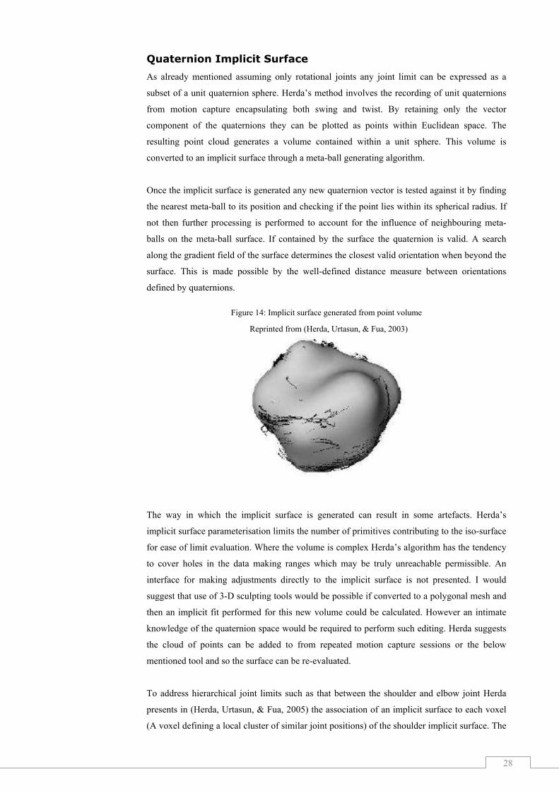
28

Quaternion Implicit Surface

As already mentioned assuming only rotational joints any joint limit can be expressed as a

subset of a unit quaternion sphere. Herda’s method involves the recording of unit quaternions

from motion capture encapsulating both swing and twist. By retaining only the vector

component of the quaternions they can be plotted as points within Euclidean space. The

resulting point cloud generates a volume contained within a unit sphere. This volume is

converted to an implicit surface through a meta-ball generating algorithm.

Once the implicit surface is generated any new quaternion vector is tested against it by finding

the nearest meta-ball to its position and checking if the point lies within its spherical radius. If

not then further processing is performed to account for the influence of neighbouring meta-

balls on the meta-ball surface. If contained by the surface the quaternion is valid. A search

along the gradient field of the surface determines the closest valid orientation when beyond the

surface. This is made possible by the well-defined distance measure between orientations

defined by quaternions.

Figure 14: Implicit surface generated from point volume

The way in which the implicit surface is generated can result in some artefacts. Herda’s

implicit surface parameterisation limits the number of primitives contributing to the iso-surface

for ease of limit evaluation. Where the volume is complex Herda’s algorithm has the tendency

to cover holes in the data making ranges which may be truly unreachable permissible. An

interface for making adjustments directly to the implicit surface is not presented. I would

suggest that use of 3-D sculpting tools would be possible if converted to a polygonal mesh and

then an implicit fit performed for this new volume could be calculated. However an intimate

knowledge of the quaternion space would be required to perform such editing. Herda suggests

the cloud of points can be added to from repeated motion capture sessions or the below

mentioned tool and so the surface can be re-evaluated.

To address hierarchical joint limits such as that between the shoulder and elbow joint Herda

presents in (Herda, Urtasun, & Fua, 2005) the association of an implicit surface to each voxel

(A voxel defining a local cluster of similar joint positions) of the shoulder implicit surface. The

Reprinted from (Herda, Urtasun, & Fua, 2003)

29

storage of the many required child implicit surfaces makes this solution somewhat unwieldy

and again given the shapes of the surfaces it would be difficult for a user to intuit the limits

visually.

Figure 15: Voxelised shoulder surface and associated child surfaces

While Herda uses a tool known as “WinSceneGraph” this program does not seem to appear in

the public domain. I am basing any conclusion about this tool based solely on the user manual

of this application found at http://vrlab.epfl.ch/~lorna/docs/WinSceneGraph.pdf. Its main

function seems to be the processing and conversion of point clouds as generated from motion

capture or loaded from a file. Point clouds may be expressed in Quaternion or Cartesian

formulations. The tool seems to permit the addition of points to a data cloud by entry of

rotation values. Whether these values can be entered through a visual posing of an armature is

unclear. The tool generates the required values for an implicit surface. Whether this surface can

be displayed and intuitively edited within the tool interface is also unclear. See appendix

(pg.56, Figure 44) for list of conversion menu functions.

Reprinted from (Herda, Urtasun, & Fua, 2005)

30

Joint sinus accumulation buffer

The approach most similar to my own is presented by (Jing & Prakash, 2000) and utilises a

Theta Phi decomposition of all valid vectors of a joint sinus to an accumulation buffer reducing

point within bounds test to a simple lookup with binary result. They do not seem to consider

the graphical editing of the accumulation buffer as a texture. Their approach also makes no

attempt to encode permissible twist.

Figure 16: Phi Theta decomposition of a point within joint sinus.

Quaternion based accumulation buffer

(Liu & Prakash, 2003) use a standard unit quaternion parameterisation in their work. However

while stating that rotation limits form a region in 3-sphere they only discuss the workings of a

swing limit and do not address twist.

Their formulation of a look-up table differs from my own. Their method can be summarised as

follows: To rotate from a reference vector (a) to another (b) an axis of rotation (u) is utilised. u

is unit length and generated from cross product of a and b. The range of motion is restricted by

placing a limit on the permissible rotation about any given u.

If a is chosen to be the z-axis then u which lies on the orthogonal plane XY can be

parameterised with and angle Φ measured counter clockwise from the positive x-axis. Φ can be

quantised 0 to 360 degrees. The permissible rotation about u is encoded as a value between

zero to one, the result of the cosine of half the angle, and so the below look-up can be

generated.

Reprinted from (Jing & Prakash, 2000)

31

Figure 17: Limit look-up table. Area is yellow is the valid range.

I consider this formulation very novel and may adopt it in future work however twist is not

discussed in their work (though clearly could be addressed in the same manner I will propose).

Nor are the other benefits made possible through a discretisation of limit boundaries that I will

be presenting.

Summary

While lookup tables have been found in existing research their description as a texture suitable

for GPU execution has not. With the exception of Herda’s work no approach solves the

dependency of twist and swing in a satisfactory manner. While a sinus cones are conceptually

intuitive Herda’s implicit surface representation is by far the most complete joint limiting

system currently in existence. The use of a quaternion rotation formulation is desirable. Tools

in this space are sparse and not publically available.

Reprinted from (Liu & Prakash, 2003)

32

Artefact Design and Implementation

Methodology

It was intended that a prototype extension to the Blender 3-D package be created to act as a test

bed for a texture based joint limit solution. The standard Blender install currently only permits

Euler angle rotation limits. To show that my system is an improvement over this a comparison

of permitted range of motion is to be performed.

Detailed timing information of existing techniques is not provided in many of the papers upon

which my literate review was based and so hampers a comparison. As the proposed system is

intended for GPU execution a shader program written in the High Level Shading Language

standard (HLSL) is used for evaluation. Though use of the FX Composer 2 shader analysis tool

from NVIDIA, a count of the functions required and their timing information can be obtained.

From this it should be determinable if the solution is computationally prohibitive or not for its

application in a video game execution environment.

Prototype Programming

A rapid development approach was adopted with continuous revisions to the system being

created throughout the research timeline. Programming was performed in the C programming

language. Python scripting was often used to test ideas but was later converted to equivalent C

code. Microsoft’s Visual C++ Express Edition was the development environment used.

Angle Parameterisation

“The swing-and-twist parameterisation is useful for dealing with ball-and-socket joints, and is

a good basis for the definition of simple yet meaningful joint limits” (Baerlocher & Boulic,

2001). For this reason it is the swing-and-twist parameterisation which is the basis of the

solution though where possible quaternions are used where interpolation is required.

33

Virtual Body Modelling

A detailed polygon mesh of a human male was modified to provide a suitable character for

manipulation. The entire mesh consists of nearly 8000 vertices creating over 14000 faces.

Within this mesh the character forearm, upper arm and torso are separate mesh loops. This

separation was performed to enable easy selection of vertices for bone influence assignment

and also to remove consideration of possible skinning issues which while addressable in

Blender through dual quaternion skinning are not the focus of this research.

Figure 18: Character Mesh

Skeleton Modelling

A simple armature was constructed within the mesh (Figure 19) of a similar design to that seen

in video game characters (pg.58, Figure 51). The creation of the armature rig with arms

outstretched from the body is a commonly used in video game character assets and is referred

to as the initial “T pose”.

Figure 19: Character armature

Model Posing

As shown in (Figure 20) once vertex-bone associations have been created the existing features

of Blender permit the posing of the armature bones to affect the character mesh posture.

However the existing mechanism for posing the armature bones through direct entry of rotation

34

angles or use of the rotation manipulator is considered unwieldy particularly as the trackball

movement (pg. 56, Figure 45) seen in other packages appears absent from Blender. To address

this problem a UI element was developed (Figure 21) which was derived from a Blender UI

element used for setting lighting directions and was named the “pose helper”. Through

interaction with the 2-D sphere via the mouse the direction vector (swing) of the selected bone

could be set. For the upper-arm bone with the red circle of the pose helper obscuring the black

circle the pose would be set to the default T position as in (Figure 19). When the direction

vector is within the opposite hemisphere to the T pose this is indicated to the user by changing

the colour of the vector line and circle to blue (See right Figure 21).

Figure 20: Armature posing

Figure 21: Pose Helper

The vector returned from the pose helper UI was converted to an armature bone pose as

follows. First the rotation about a fixed axis was calculated (Positive Y was chosen). This is

done by calculating the arc cosine of the dot product of the two vectors. Then the orthogonal

vector to each vector was calculated by using the cross product. This allows formulation of

pose as a Vector and Rotation which is easily converted to quaternion form (Appendix pg.59).

In Blender each bone has a quaternion parameter. Having set the quaternion all that is required

is to call a recalculation of pose matrices and call a draw function to display the result on

screen.

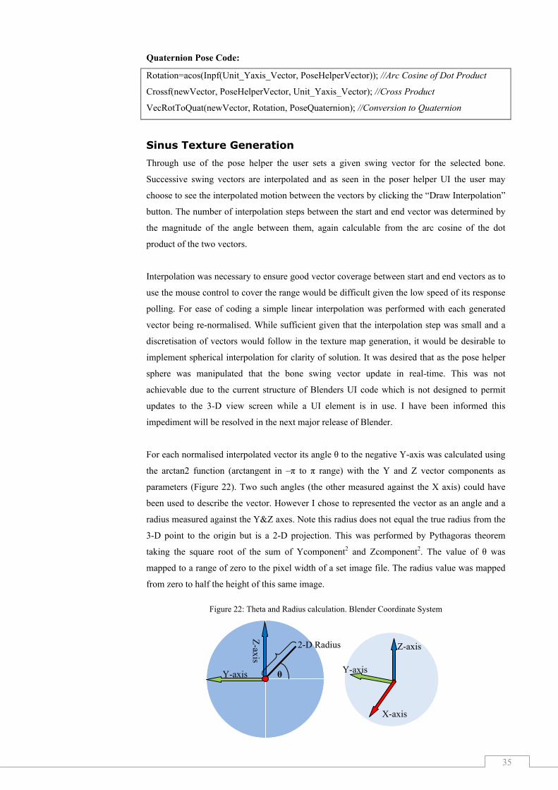
35

Quaternion Pose Code:

Rotation=acos(Inpf(Unit_Yaxis_Vector, PoseHelperVector)); //Arc Cosine of Dot Product

Crossf(newVector, PoseHelperVector, Unit_Yaxis_Vector); //Cross Product

VecRotToQuat(newVector, Rotation, PoseQuaternion); //Conversion to Quaternion

Sinus Texture Generation

Through use of the pose helper the user sets a given swing vector for the selected bone.

Successive swing vectors are interpolated and as seen in the poser helper UI the user may

choose to see the interpolated motion between the vectors by clicking the “Draw Interpolation”

button. The number of interpolation steps between the start and end vector was determined by

the magnitude of the angle between them, again calculable from the arc cosine of the dot

product of the two vectors.

Interpolation was necessary to ensure good vector coverage between start and end vectors as to

use the mouse control to cover the range would be difficult given the low speed of its response

polling. For ease of coding a simple linear interpolation was performed with each generated

vector being re-normalised. While sufficient given that the interpolation step was small and a

discretisation of vectors would follow in the texture map generation, it would be desirable to

implement spherical interpolation for clarity of solution. It was desired that as the pose helper

sphere was manipulated that the bone swing vector update in real-time. This was not

achievable due to the current structure of Blenders UI code which is not designed to permit

updates to the 3-D view screen while a UI element is in use. I have been informed this

impediment will be resolved in the next major release of Blender.

For each normalised interpolated vector its angle θ to the negative Y-axis was calculated using

the arctan2 function (arctangent in –π to π range) with the Y and Z vector components as

parameters (Figure 22). Two such angles (the other measured against the X axis) could have

been used to describe the vector. However I chose to represented the vector as an angle and a

radius measured against the Y&Z axes. Note this radius does not equal the true radius from the

3-D point to the origin but is a 2-D projection. This was performed by Pythagoras theorem

taking the square root of the sum of Ycomponent2 and Zcomponent2. The value of θ was

mapped to a range of zero to the pixel width of a set image file. The radius value was mapped

from zero to half the height of this same image.

Figure 22: Theta and Radius calculation. Blender Coordinate System

θ Y-axis

Z-ax

is

Y-axis

Z-axis

X-axis

2-D Radius

36

During testing an image of 256 x 512 pixels was used. Radii of vectors with a positive X

component take up the bottom half of the image with the radius lengths from zero to one

mapped to pixel height 0 to 255 measured from the bottom. While the radii of vectors with a

negative X component occupy the top half with lengths of one mapped to the mid height of the

image and 0 at the image top. The image space can be considered to be divided into two

hemispheres.

Point within boundary test

To determine if a given swing vector is within the sinus boundary its x and y pixel coordinates

are calculated as above. If the pixel value of the red channel is 0 at those coordinates then the

point is invalid otherwise the vector is within the sinus cone and considered valid. Such a pixel

look up is computationally inexpensive for modern GPUs and will be discussed later.

Figure 23: Sinus Cone Texture

Dotted line is

Hemisphere

Boundary

Black = Invalid Swing Region

Red = Valid Swing Region

256

256

256

0

1

0

Neg

ativ

e X

co

mp

onen

t:

Rad

ius

Len

gth

Po

siti

ve

X c

om

po

nen

t:

Rad

ius

Len

gth

Theta (θ) ranging from zero to 2π

37

Sampling issue with the texture

While the 255 vertex points for the sinus cone is significantly more than that seen tested in

other research the proposed system necessitates that the points be evenly distributed. Regions

of high gradient change may not be sampled sufficiently. Rather than a somewhat smooth pixel

curve a significant step effect of pixels is seen in these areas. This is addressed somewhat

through higher resolution textures but I have not presented a means to increase the number of

vertices in an area. The concentration of vertices is adjustable in existing research. To consider

these steps as control points for a curve could be explored however the advantages of a simple

pixel boundary test are then removed.

Figure 24: Zoom in on pixel step effect

Sinus Cone Visualisation

While a texture rather than a 3-D sinus cone is used in limit calculation I consider sinus cones a

useful visual representation of swing limits. For this reason I decided that displaying the sinus

cone would be of benefit particularly for users already familiar with such a representation. To

do so a polygon cone with non closed circular base having a number of vertices equal to width

of the sinus texture was generated, with one vertex being the apex. Then through finding the

pixel height value of the red/back pixel boundary for each image column and converting these

x and y pixel coordinates back to vector form a 2-D array of vectors was generated. The vertex

array of the circular base cone was then set to this 2-D array producing the sinus cone as shown

in (Figure 25).

Conversion from 2-D Pixel coordinates back to a Vector:

float Vector[3]; float recoveredRadius; float theta=(x*(2.0f*(float)M_PI))/((float)width); if (y>(height/2)) {

y=(height-y); recoveredRadius=((float)y)/((float)(height/2)); Vector[2]=-(sqrt(1.0f-(recoveredRadius*recoveredRadius))); } else { recoveredRadius=((float)y)/((float)(height/2)); Vector[2]=sqrt(1.0f-(recoveredRadius*recoveredRadius)); } Vector[0]=(cos(theta))*recoveredRadius; Vector[1]=(sin(theta))*recoveredRadius;

38

Figure 25: Circular Base Cone and resulting Sinus Cone

Sinus Boundary Animation

A button was provided for the user to see the effect of the sinus boundary causing the selected

joint to move through the 255 vector positions of the boundary. Interpolation while easily

implementable was not considered necessary for this visualisation. It is noted however that as

expected from (Figure 24) the animation is not of a constant acceleration. Discontinuities occur

as no interpolation based on a distance measure between vertices is being performed here.

Figure 26: UI Panel and Boundary Animation

Editing of Sinus Texture

Blender already has basic pixel painting tools. To aid in the editing of the sinus texture two

brushes were setup for convenience to paint black and red pixels onto the texture. A contiguous

area of black was not enforced and so holes could be created which would be analogous to

non-overlapping spherical polygons (See Appendix pg.59, Figure 52). Though as noted in

(Baerlocher & Boulic, 2001) such holes are perhaps unnecessary for human joints. For ease of

use any future development should perhaps ensure only two distinct regions are created. The

creation of overhangs is also possible (Right Figure 27). The Sinus cone of (Figure 25) can be

updated to match texture boundary by clicking the “Test JLC” button of (Figure 26).

Figure 27: Pixel editing tool

Run Animation

Paint as left mouse clicked Overhang Hole

39

Consideration of Limit avoidance and Stress Measurement

The texture format for the sinus limit provides a convenient mechanism to also encode stress or

the encroachment upon the boundary curve. As will be presented with twist, values could be

set at key joint articulations and interpolated. These key values could set through presenting a

slider bar UI and may be based on feedback of discomfort from a live subject. However given

the intuitive mapping of the texture a painting of stress with pixel tools was approached. White

was used as the colour to indicate a high stress level with black being considered no stress

(Figure 28). A graduation was performed respecting the boundary curve. This gradient map

could be integrated into an Inverse Kinematics (IK) system performing least resistance path

finding. Also shown in blue (Figure 28) the degree to which the boundary could be exceeded

before a change of simulation would be required can also be mapped. This was intended to be

used to show when a joint would be broken had a force from a physics system placed the joint

in such an orientation.

While Blender provides a way to set soft edge brushes the stress map generation process is

more suited to dedicated graphics editing package such as Adobe Photoshop were gradient

generation tools may be of benefit.

Figure 28: Stress Map

Correction of point beyond boundary

Considered in isolation

If presented with a vector beyond the sinus boundary and no consideration is given to any

previous vector then at that vectors pixel position a reference to its nearest valid boundary

point can be pre-computed. Given that a pixel in the joint limit texture that has a zero red

channel value is considered out of the sinus bounds then the green, blue and alpha channel of

that pixel are unutilised. If the Green channel 0-255 is used to directly index the X position of

the nearest valid boundary pixel then the addition of the blue and alpha channel values can

index the Y position (0-511) of the valid boundary point (Figure 29 right)

Noting that offline computation can be as complex as desired to find the nearest valid boundary

point a temporary array of all boundary pixels was constructed. The angle between the

corresponding vector of each entry of the array and the vector of the point beyond bounds was

Low Stress - High Stress

calculated (Ar

joining the two vectors

was stored.

not deemed suitable given the curvature of the true space

Having performed a

channel value the correcti

conversion of the vector to

by that pixel

pix

limitation of 8

nearest point

Should the exact corrective boundary pixel not be index able then at

searc

to the boundary

number on either side of the point in the horizontal. The projected boundary

lowest pixel distance to the invalid point becomes the start point of a boundary search. The

direction along the boundary is followed while the distance to invalid point is reducing and so

corrective point is converged upon (

calculated (Ar


was stored.


Having performed a



by that pixel

pixels or less

limitation of 8

nearest point


searc

to the boundary





calculated (Ar


was stored.


Having performed a



by that pixel

els or less

limitation of 8

nearest point


search w

to the boundary





calculated (Ar


was stored.


Having performed a



by that pixel

els or less

limitation of 8

nearest point


h would be performed as follows.

to the boundary





calculated (Arccosine of Dot Product)


was stored. A


Having performed a



by that pixel. This is considered highly efficient and easily achieved for an image of

els or less. A

limitation of 8

nearest point to


ould be performed as follows.

to the boundary





ccosine of Dot Product)


A 2-D


Having performed a



. This is considered highly efficient and easily achieved for an image of

. At larger texture dimensions (unless split into multiple textures)

limitation of 8-bits per pixel channel it may only be possible for

to be referenced and so require a subsequent local



to the boundary (just downward if pixel overhangs are not permitted)







D pixel distance


Having performed a




t larger texture dimensions (unless split into multiple textures)

bits per pixel channel it may only be possible for

be referenced and so require a subsequent local



(just downward if pixel overhangs are not permitted)






joining the two vectors (Figure

pixel distance


pre-















Figure

pixel distance


-comput

channel value the correction of a

conversion of the vector to a





Figure

Figure









Figure

pixel distance


comput

on of a

a pixel lookup and a conversion back





Figure

Figure









Figure 29 left)

pixel distance measure


computation

on of a

pixel lookup and a conversion back





Figure 29: Arc

Figure 30: 2









left)

measure


ation

on of a vector






: Arc

: 2-D distance measure Pre







corrective point is converged upon (Figure

ccosine of Dot Product). The angle in radi

left). A reference to the pixel yielding the smallest length arc

measure


for each pixel of the joint limit texture with a zero red

vector






: Arc distance measure Pre

D distance measure Pre


ould be performed as follows. The number of pixels to cast the invalid point vertically





Figure

The angle in radi

A reference to the pixel yielding the smallest length arc

measure was also



vector beyond the sinus boundary simply involves the






distance measure Pre



he number of pixels to cast the invalid point vertically





Figure 31

The angle in radi


was also



beyond the sinus boundary simply involves the














31 right).

The angle in radi


was also

















right).

The angle in radi


was also programmed

















right).

The angle in radi


programmed

not deemed suitable given the curvature of the true space (








distance measure Pre-

D distance measure Pre-







The angle in radians is


programmed

(Figure








-computation

-computation







ns is


programmed

Figure







be referenced and so require a subsequent local sear

computation

computation







equal to the length of the arc


programmed for testing purposes

Figure 30)



to a vector of the value stored



bits per pixel channel it may only be possible for a point in the region of the

search.

computation

computation









for testing purposes

)






a point in the region of the

ch.

computation

computation
















Should the exact corrective boundary pixel not be index able then at run time


(just downward if pixel overhangs are not permitted) is recorded as is the













run time


is recorded as is the













run time



number on either side of the point in the horizontal. The projected boundary point having the










t larger texture dimensions (unless split into multiple textures) due to the


run time the localised



point having the





for testing purposes but was




. This is considered highly efficient and easily achieved for an image of 256x512

due to the


the localised



point having the





but was




256x512

due to the


the localised



point having the



40



but was




256x512

due to the


the localised



point having the


direction along the boundary is followed while the distance to invalid point is reducing and so a

40



but was




256x512

due to the


the localised



point having the


a

41

Figure 31: Binary Search Boundary Correction

Considered with known last valid position

If an animation has a previous valid swing position and new invalid swing position then it is

assumed any interpolation between these points would occur along a great arc between them.

This great arc would intersect the boundary curve and the intersection point should be the

corrective boundary position. A binary search along this curve is proposed to converge on the

crossing point at runtime which is to be the corrective boundary position but was not

implemented in the artefact. The midpoints would be generated from interpolating linearly

between the vectors and renormalizing the resultant vector, exact midpoints may not be created

but that is not of concern to the algorithm. As shown in (Figure 31) the successive midpoints

(1-5..) would be tested as per binary search rules and so a pixel that is valid but has one or

more surrounding pixels that are invalid is converged upon. It is noted that this does not

guarantee that the first crossing of the boundary is found as shown in (Figure 32).

Figure 32: Possible error with binary search

.

While the number of steps required for search will vary for different last and new positions I

will later show that the GPU can perform such tests highly efficiently.

Found through

Binary search

*

42

Concave Boundary Jumping

“A great arc connecting two points may not be fully contained in the valid region, even if the

two extremities are” (Baerlocher & Boulic, 2001). This may cause an abrupt movement from a

valid region to another, which are close in space but that require a long path to be connected

(Baerlocher & Boulic, 2001). As suggested by Baerlocher we can minimize the effect of

boundary jumping by testing the midpoint. If the midpoint is invalid the lookup of the pre-

computed nearest boundary position to that mid point makes this approach highly efficient and

could be repeated several times to better follow the boundary curve. If required an exhaustive

pixel search could also be performed to trace the boundary between the points.

Figure 33: Avoidance of Boundary Jumping

Setting Twist

An existing method to set the bone twist was possible through interaction with the y-axis of

Blenders standard rotation manipulator orientated to the bone normal. However the picking of

this axis with the mouse was often hindered by the presence of the other axes and so a more

user friendly UI was developed (Figure 34). The other axis where removed and a partial disk

was displayed indicating the angle of twist against the vertical zero twist position. This UI

enabled the recording of the permissible minimum and maximum twist limit for a given swing

vector either side of the zero position (each displayed in a differing shade of green). An

interaction restriction of up to 180 degrees in either rotation direction was imposed. Through

visual observation this was considered sufficient to capture human limits.

Figure 34: Twist setting UI

43

Encoding and Interpolation of Twist

Figure 35: Interpolation of Twist

Through encoding the clockwise maximum twist for a given swing vector in the red channel (0

red being reserved) and the maximum anticlockwise twist in the green channel the lookup of a

swing vector in the texture map yields the permitted twist. The values of permitted twist should

be obtained from motion capture however as values for the whole discretised pixel range of

swing would be laborious to obtain some form of interpolation would be desirable to fill data

holes. Time constraints did not permit the scheduling of motion capture session and so as a

substitute the twist freedom of my own arm at key positions were simply observed and

replicated visually through use of swing and twist setting UIs. The values were then

interpolated horizontally to form bands (B) and (C) as shown in (Figure 35). Similarly key

twist limit points along the boundary curve were interpolated along the boundary (A) and the

value of permitted twist at the initial T pose was also recorded (D). A vertical interpolation

between bands was then performed followed by a 2-D convolution on the red and green

channel separately to smooth the values resulting in the image to the right in (Figure 35). To

save programming time this convolution was achieved in Photoshop rather than within

Blender. It should be noted that their many bands could be created for greater accuracy.

Elbow shoulder Hierarchy

In certain cases to consider the range of motion of joints as independent would result in

impossible poses, for example the shoulder and elbow joints could permit the hand to penetrate

the chest. To capture the coupling that exists between the ranges of motion between multiple

joints the following (while unimplemented) is proposed for the elbow shoulder hierarchal

rotation limits. A 2-D array of the same dimensions as the joint limit text could be constructed.

A further dimension would be added (Now 3-D), ranging from the maximum of any possible

Interpolated Twist

(A) Boundary Twist Values

(B) Circumference 1 Values

(C) Circumference 2 Values

(D) Centre point single value

A

B C

D

44

anticlockwise shoulder twist through to the maximum of any possible clockwise shoulder twist

at some fixed discretisation for a given swing (2-D correspondence with the texture).

The value stored at the 3-D position would be the permitted angle range for the elbow from the

zero rotation of the elbow (inline with upper arm). The 3-D array is accessed by converting a

given swing to its 2-D pixel coordinates as before and using the twist value of the shoulder to

index to the permitted 1-D rotation value of the elbow. It is recognised that this is a very large

and wasteful array structure. A lower resolution array may be sufficient such as could be

achieved by scaling in half the array size in the first two dimensions. This would be indexed by

diving the vector swing pixel coordinates by two and then indexing the twist value.

Figure 36: 3-D Hierarchy array

Procedure for respecting limits

• Convert the proposed orientation into its equivalent swing-twist components.

• A test is performed to determine if the swing component is within its range of motion

followed by testing of twist.

• If swing is beyond its range that is first resolved through location of the closest point

on the boundary curve to the proposed swing orientation. Pre-computed point is used

if considered in isolation, otherwise binary search is performed.

• Twist is then resolved if beyond its limits.

• If a hierarchal elbow limit is to be respected its value is corrected to the nearest

permitted value as obtained for a given shoulder swing and twist from a 3-D array.

Texture Formats

The dimensions of 256 x 512 were chosen so the image could be spit into two square images as

equal power of two dimensioned textures were a format requirement for previous generations

of GPUs. It is notable that if the sinus cone boundary were all that the study was concerned

with then the braced range of interest shown in (Figure 23) could be contained within a single

256x256 image. Red was the chosen colour for the permissible swing region as it was

considered that as red is the first entry of and RGB image it would be the quickest to index into

though some image formats do in fact reverse the RGB order.

Elbow rotation values

stored at third dimension

of array.

The tested joint limit texture with dimensions of 256x512 encoding swing and tw

single joint has a file size of 25.3KB when using a png24 format

file size is achieved because only two channels are utilised

of the

were all that was required a binary image could be used.

If a stress map is desired the blue channel can be occupied by the greyscale seen in (

The green

computed boundary positions and so a 32

Pixel areas within the boundary curve do not utilise the alpha channel.

is recognised

textures can often be several MBs in size optimisation was not a considered necessary.

already discussed the reason for use of the alpha cha

range and

would not be required.

The GPU will not process an image in png format and so a conversion is required. To support a

hierarchal limit all four channels are required. An unsigned 32

format is 512KB in file size. The

interpolated non

(128KB)




of the



The green



is recognised



range and



ierarchal limit all four channels are required. An unsigned 32


interpolated non

(128KB)




of the blue channel



The green



is recognised



range and





interpolated non

(128KB)




blue channel



The green,



is recognised



range and therefore





interpolated non

(128KB) but its effect on




blue channel



blue and alpha chann



is recognised this



therefore





interpolated non

but its effect on




blue channel






this



therefore





interpolated non-pre

but its effect on

Shown with blue channel stress map within valid swing region.




blue channel is simple for the png compress






this is still wasteful as an RGB format would be smaller, but as video game



therefore should the texture be split into squares of a 256x256 dimension then it





pre-multiplied alpha and may offer sufficient quality at a much small

but its effect on





is simple for the png compress






is still wasteful as an RGB format would be smaller, but as video game



should the texture be split into squares of a 256x256 dimension then it





multiplied alpha and may offer sufficient quality at a much small

but its effect on



















but its effect on the



















the accuracy of system has not been explored

Figure


Alpha channel values are not shown.







blue and alpha channel for pixels with a zero red value are used for indexing pre











accuracy of system has not been explored

Figure









el for pixels with a zero red value are used for indexing pre












Figure 37


















format is 512KB in file size. The DXT5



37: Final Joint Limit Texture










computed boundary positions and so a 32-bit png is required (8bits per channel)








DXT5



Final Joint Limit Texture










bit png is required (8bits per channel)








DXT5 format is a compressed texture format with





















format is a compressed texture format with









is simple for the png compression technique.








already discussed the reason for use of the alpha channel is to aid in the indexing of the height













ion technique.








nnel is to aid in the indexing of the height












file size is achieved because only two channels are utilised (red and green)

ion technique.



















(red and green)

ion technique.


















single joint has a file size of 25.3KB when using a png24 format without alpha channel

(red and green)

ion technique. If a swing limiting texture










ierarchal limit all four channels are required. An unsigned 32-bit RGBA texture in DDS







without alpha channel

(red and green)

If a swing limiting texture




Pixel areas within the boundary curve do not utilise the alpha channel. The






bit RGBA texture in DDS



accuracy of system has not been explored.




(red and green)





The












and so compression





The file size is 61KB.










The tested joint limit texture with dimensions of 256x512 encoding swing and twist limits for a


and so compression





file size is 61KB.










ist limits for a


and so compression


If a stress map is desired the blue channel can be occupied by the greyscale seen in (Figure


bit png is required (8bits per channel) (Figure

file size is 61KB.









ist limits for a


and so compression


Figure


Figure

file size is 61KB.









ist limits for a

without alpha channel. This

and so compression


Figure 28


Figure 37

file size is 61KB.








multiplied alpha and may offer sufficient quality at a much smaller size

45

ist limits for a

. This

and so compression


28).

el for pixels with a zero red value are used for indexing pre-

37).

file size is 61KB. It


textures can often be several MBs in size optimisation was not a considered necessary. As






er size

45

ist limits for a

. This

and so compression


).

-

.

It


s






er size

46

Alternative Avenue of Investigation

Research toward encoding an implicit surface to texture

The initial focus of my research was to investigate if a cube map texture could be used to

encode an approximation of Herda’s implicit surface to represent joint limits. It was hoped that

the representation obtained from imaging Herda’s 3-D surface from six directions would be

sufficiently accurate at reasonable texture dimensions for the reconstruction of the surface to

within a workable tolerance. An orthographic projection from each pixel of a cube face to the

3-D surface would obtain a depth value to be encoded into the colour channels of that pixel.

As already mentioned Herda’s implicit surface parameterisation limits the number of

primitives contributing to the iso-surface for ease of computation. If an image of the iso-

surface is all that need be retained the surface can be as complex as desired.

During the manipulation of the armature bones quaternions were generated and appended to a

text file. Code was written to take this list of quaternion 3-D coordinates and generate a small

meta-ball for each entry of a set radius as apposed to Herda’s method where meta-balls

encompass multiple quaternion points. A distance measure was created to ensure quaternions

already contained within a meta-ball be excluded. It was envisioned that this would largely

overcome the problem of unwanted hole filling as seen in Herda’s system and also not produce

a largely smooth surface unless the data supported it.

It was hoped such a system would reduce Herda’s surface inclusion test of a 3-D point

(representing simultaneously a swing and twist) to a lookup of the corresponding pixel for each

face of the cubemap. It was expected that the computation needed to yield the result would be

significantly less than that for Herda’s approach.

Figure 38: Visualisation of cube-map

In exploration of this approach a pipeline was created within Blender to image a depth map of

an implicit surface from a given camera position. Through use of this pipeline it was intended

that the camera be positioned appropriately and the Cube-map be constructed from six such

depth maps.

47

Figure 39: Depth map pipeline

The above depth map takes no account of the internal structure of the implicit surface, only

imaging its outer hull. Any caverns within the surface which denote invalid rotations must be

accounted for. To do so I propose that the surface be converted to a polygon mesh as in (Figure

40). Through selection of a face on the surface of this polygon mesh all connected faces can be

found and deleted. Blender has an inbuilt function for such connected face searches as seen in

the menu shown in (Figure 40). This leaves only the faces not connected to outer hull and so

encompass holes in the surface. A depth map of the holes can then be constructed. It was

intended that the outer surface depth maps and holes depth maps be composited into different

colour channels of the cube-map.

While I consider the major elements required for this approach complete, due to time

constraints I had not addressed an intuitive means to edit the surface, represented hierarchal

limits or resolve the boundary for points beyond limits. For these reasons I decided it would be

more fruitful to pursue a more complete and user-friendly system without an implicit surface

base.

Figure 40: Obtaining holes in surface

Implicit Surface Greyscale Depth

Implicit Surface Polygon Surface

Result of linked face removal

from polygon surface

Select linked

faces

48

Results

Comparison of boundaries

The boundary possible through placing a minimum and maximum angle limit on each DOF as

possible in Blender and other 3-D packages is visualised in (Figure 41 left) with the swing

range being the carved out area of the sphere.

Figure 41: Min Max limits of each DOF vs Texture Swing Limit

“Such a representation may be considered sufficient for mechanical simulations in general, it

may not lead to realistic postures concerning the vertebrate bodies, especially the human body”

(Maurel, 2000). Maurel recognises that sinus cones are a significant improvement over such a

representation. Given that the proposed texture sinus boundary is at its base a different means

to describe a sinus cone its properties to better describe the human range of motion similarly

applies (Figure 41 right).

Execution Performance

High Level Shading Language (HLSL) is a proprietary shading language developed by

Microsoft for use with the Microsoft Direct3D API. A HLSL shader was written to test the

performance of the proposed algorithms for “point within boundary test” (Code 2 pg60) and

“point beyond boundary correction”. No impediments exist for a similar shader to be written

for the OpenGl standard. The NVIDIA GeForce 6600 GT is Mid-Range GPU launched in

September 2004. With a launch price of $199 it is considered a mainstream product. This GPU

was chosen as a benchmark as its performance is comparable to that present in the current

generation of video game console.

Profile of NVIDIA GeForce 6600 GT GPU

Memory Interface 128-bit

Memory clock speed 1.0 GHz GDDR3

Core 500 MHz

Pipes 8

49

Reporting from NVIDIA FX COMPOSER 2:

FX Composer is an integrated development environment for shader authoring and provides

tools for shader performance analysis across multiple GPUs. Using FX Composer the “point

within bounds test” compiled with ps_3_0 requires 34 assembly instruction slots, 1 texture

allocation and 33 arithmetic functions. Two registers are used. The operations completes in 15

Cycles when using FP16 precision and 16 Cycles at FP32 precision. 15-16 Cycles is a very

minimal amount of processing and once the texture is loaded into the GPU memory

communication with the CPU would be minimal in this system. A more experienced shader

programmer would also likely be able to optimise the shader for enhanced performance.

Table 1: Boolean Test Shader Simulated Results

GPU Driver Type Cycles Registers

GeForce 6600 GT* 163.2 fragment 15 2

GeForce 6800 163.2 fragment 15 2

GeForce 6800 GT 163.2 fragment 15 2

GeForce 6800 Ultra 163.2 fragment 15 2

GeForce 7800 GT

Released (August , 2005) 163.2 fragment 11 3

*Benchmark GPU

With a cycle rate of five hundred million per second and an assumed 60 tests for the shoulder

joint per second (60 fps animation) then under ideal circumstances a single test would

theoretically utilise less than 0.000002% of the GPU execution budget. While a simplification

of the nature of GPU processing this figure indicates how minimal the impact of such tests on

an execution budget are and so are deemed suitable for real time applications. The “point

beyond boundary correction” for a vector considered in isolation is also calculable in a fixed

low number of cycles. 24 Cycles for execution on the GeForce 6600 GT, 65 instruction slots

used (1 texture, 64 arithmetic).

Table 2: Corrective Shader Simulated Results

GPU Driver Type Cycles Registers

GeForce 6600 GT* 163.2 fragment 24 4

GeForce 6800 163.2 fragment 24 4

GeForce 6800 GT 163.2 fragment 24 4

GeForce 6800 Ultra 163.2 fragment 24 4

GeForce 7800 GT

Released (August , 2005) 163.2 fragment 16 4

*Benchmark GPU

The number of cycles required for a “point beyond boundary correction” with consideration of

a known previous valid vector is not fixed however its worst case could be calculated given

that the largest distance the binary search could possibly need to cover is the diagonal of the

joint limit texture: √256' ( 512'.

50

Recommendations for Further Work

Improvement to User Interface

The user interface of the tool consists of a large number of buttons many of which were simply

of use in debugging the system. A through review of the UI is required to make it more user

friendly. For users uninterested in editing limits I propose that a library of pre-generated joint

limit textures be accessible.

Acceptance of the system into blender package

The development of the system required modification to a large number of diverse systems

within blender. Due to a lack of what I would consider sufficient development documentation,

a lack of knowledge of Blenders intended development route and my unfamiliarity with the C

coding language many coding hacks were involved in the creation of this system. Updates to

the structure of the blender code base is expected in the forthcoming 2.5 release and so any

new additions must respect these changes. For these reasons a rewrite of my code is

necessitated and the system will not be submitted for consideration of inclusion within Blender

in its current form. However the Blender development and user communities have reacted most

favourably to the features proposed and eager to see their continued development and inclusion

within Blender.

Implementation of Hierarchal limits and IK integration

The coding of hierarchal limits and the integration of system into IK evaluation remains

undone. While not considered difficult to code, implementation of these features would greatly

enhance the usefulness of the system.

Mip-mapping

There may exist situations where texture memory allocation is of concern. Mipmaps would

present a means to balance this issue with accuracy of result. This could be leveraged in

simulations of large crowds of characters where if each were to have unique joint limits

(perhaps due to their armament) a characters distance from the camera could determine the

required mipmap level. This would provide a courser but more efficient lookup for distant

characters.

Continued investigation of a cube mapped implicit surface

Cubemaps are commonly used in modern computer graphics and their use is often optimised

on GPU hardware (Appendix pg.55). The quantisation of a continuous surface to pixels even at

high texture resolutions would result in some inaccuracies. While I did not address this and

several other issues such as a means to designate hierarchal limits, the cubemap appears in

principle a promising representation and I believe warrants further research.

51

Conclusion

The proposed system addresses many of features which I consider desirable for a joint limit

system.

Accuracy of result and a convenient means of limit storage

While the limits have been discretised the resolution obtained is considered sufficient for many

applications. The texture is constructed such that the singularity of axis angle parameterisation

is far from the sinus boundary. A texture format for data such as normal maps is widely used in

the video games industry and is so a familiar and convenient storage mechanism.

Need for variance from generic constraints

The proposed UI enhancements and pixel painting tools provide a convenient means to edit a

sinus boundary.

Address lack of tools

The system was developed within a popular free 3-D package and many of its features are

expected to be adopted in a public release of that software.

Joint Coupling

A 3-D array appears to be suited to capture the relationship between shoulder and elbow and

could be similarly applied to the hip and knee.

Limit avoidance and stress measurement

A stress gradient map is easily integrated into the texture format.

Requirement for real-time evaluation and resolution of limits

It is in this area that the proposed system excels as it the GPU can be utilised in the evaluation

and resolution of limits. While timing information is absent from much of the existing research

from consideration of the operations other methods require I am confident that the proposed

system outperforms them by many orders of magnitude.

I have described a method of limiting joint motion based on a texture based approximation to a

sinus cone for joints with three rotational degrees of freedom. The system addresses a means to

encode permitted twist at the level of discretisation of swing. The system provides a more

realistic range of motion than simple limits on Euler angles. Run time calculations are

performable on the GPU and are suited to real-time evaluation. The system developed is

considered to be of significant use to simulations utilising dynamics, AI or physical motion

generation.

YouTube Videos of System in Operation

http://www.youtube.com/watch?v=GWAmw6Ycu8I&fmt=18

http://www.youtube.com/watch?v=QUmFYtWTmxA&fmt=18

52

Bibliography

Aubel, A., & Thalmann, D. (2000). Efficient Muscle Shape Deformation. IFIP Conference

Proceedings; Vol. 196The Netherlands (pp. 132 - 142). Deventer, The Netherlands: Kluwer,

B.V.

Baerlocher, P., & Boulic, R. (2001). Parametrization and range of motion of the ball-and-

socket joint. Deformable Avatars (pp. 180-190). Lausanne: Kluwer Academic Publishers.

Bittar, E. T., Tsingos, N., & Gascuel, M.-p. (1995). Automatic reconstruction of unstructured

3D data: Combining medial axis and implicit surfaces. Computer Graphics Forum , 14(3):457-

468.

Bourke, P. (1987, November). Determining if a point lies on the interior of a polygon.

Retrieved 08 17, 2008, from The University of Western Australia:

http://local.wasp.uwa.edu.au/~pbourke/geometry/insidepoly/

Craig, J. J. (1989). Introduction to Robotics: Mechanics and Control. Upper Saddle River, NJ:

Pearson/Prentice Hall.

Engin, A., & Tümer, S. (1989). Three-dimensional kinematic modeling of the human shoulder

complex. Journal of Biomechanical Engineering , 107-121.

Grassia, S. F. (1998). Practical parameterization of rotations using the Exponential Map.

Journal of Graphics Tools, 3(3) , 29-48.

Guillard, G., & Magnenat-Thalman, N. (2007). Ball-and-socket joint motion description using

spherical medial representation. International Conference of the IEEE EMBS Cite

Internationale (pp. 23-26). Lyon: IEEE Computer Society Press.

Hanson, A. J. (1998). Constrained optimal framings of curves and surfaces using quaternion

gauss maps. Visualization (pp. 375-382). NC: IEEE Computer Society Press.

Herda, L., Urtasun, R., & Fua, P. (2003). Automatic Determination of Joint Limits using

Quaternion Field Boundaries. In International Journal for Robotis Research, vol.22, no. 6 ,

419-436.

Herda, L., Urtasun, R., & Fua, P. (2005). Hierarchical Implicit Surface Joint Limits for Human

Body Tracking. Computer Vision and Image Understanding Volume 99 , Issue 2 , 189 - 209.

Hodgins, J. K., O'Brien, J. F., & Tumblin, J. (1998). Perception of human motion with different

geometric models. IEEE Transactions on Visualization and Computer Graphics 4 , 307-316.

Jing, H., & Prakash, E. C. (2000). SinusCone - A ThetaPhi Algorithm for Human Arm

Animation. Proceedings of the International Conference on Information Visualisation (p. 318).

London, England: IEEE Computer Society Washington, DC, USA.

Kavan, L. (2008). Geometric Skinning with Approximate Dual Quaternion Blending. ACM

Transactions on Graphics .

53

Korein, J. U. (1985). A Geometric Investigation of Reach. Cambridge: The MIT Press.

Lee, S.-H., & Terzopoulos, D. (2008). Spline Joints for Multibody Dynamics. ACM

Transactions on Graphics. New York: ACM.

Liu, Q., & Prakash, E. (2003). The Parameterization of Joint Rotation with the Unit

Quaternion. VIIth Digital Image Computing: Techniques and Applications (pp. 409-418).

Sindey: CSIRO Publishing.

Maurel, W. (2000). Human Upper Limb Modeling including Scapulo-Thoracic Constraint and

Joint Sinus Cones. Computers & Graphics, Pergamon Press, 24(2) , 203 - 218.

Ramamoorthi, R., & Barr, A. H. (1997). Fast Construction of Accurate Quaternion Splines.

International Conference on Computer Graphics and Interactive Techniques (pp. 287 - 292 ).

Los Angeles: ACM Press.

Schmidt, J., & Niemann, H. (2001). Using Quaternions for Parametrizing 3–D Rotations in

Unconstrained Nonlinear Optimization. Vision, Modeling,and Visualization 2001 (pp. 399–

406). Stuttgart, Germany: AKA/IOS Press, Berlin.

Shao, W., & Ng-Thow-Hing, V. (2003). A General Joint Component Framework for Realistic

Articulation in Human Characters. Symposium on Interactive 3D graphics (pp. 11-18).

Monterey, California: ACM New York.

Shoemake, K. (1985). Animating rotation with quaternion curves. Computer Graphics

SIGGRAPH 1985 volume 19 (pp. 245-254). San Francisco: ACM press.

Tolani, D., Badler, N., & Gallier, J. (2000). A kinematic model of the human arm using

triangular b'ezier spline surfaces.

Wang, X., Maurin, M., Mazet, F., De Castro Maia, N., Voinot, K., Verriest, J., et al. (1998).

Three-dimensional modelling of the motion range of axial rotation of the upper arm. Journal of

Biomechanics 31(10) , 899-908.

Wilhelms, G. (2001). Fast and Easy Reach-Cone Joint Limits. Journal of Graphics Tools (6)2 ,

27–41.

Wrotek, P., Jenkins, O. C., & McGuire, M. (2006). Dynamo: dynamic, data-driven character

control with adjustable balance. Proceedings of the 2006 ACM SIGGRAPH symposium on

Videogames (pp. 61-70). Boston, Massachusetts: ACM New York, NY, USA.

Zhao, J., & Badler, N. (1989). Real time inverse kinematics with joint limits and spatial

constraints. University of Pennsylvania: Technical Report MS-CIS-89-09, Department of

Computer and Information Science.

54

Appendix

Figure 42: Complete UI

55

The anatomical structure of the shoulder complex

Figure 43: The left shoulder

Acromioclavicular joints, & the proper

ligaments of the scapula

Complex nature of shoulder

This image is in the public domain because its

copyright has expired.

Simplification to a ball and socket joint

Reproduced from Biomechanical Basis of

Human Movement by Joseph Hamill and

Katheen M. Knutzen, Williams & Wilkins

1995, ISBN: 0-683-03863-X

The use of texture lookups in the graphics field

Modern graphics processing units (GPUs) expose many of the same operations supported by

CPUs through parallel programmable shaders. As computations involved in the processing of

3D graphics (the primary function of a GPU) make extensive use of matrix and vector

operations other applications reliant on such structures may be suited to GPU rather than CPU

execution. The GPU is increasingly being used for more general purpose non-graphical

calculations.

A commonly used means to map and stream data to the GPU for such applications is a two

dimension grid of values. This fits naturally with the traditional texture rendering model

supported by the GPU. The GPU memory holds these data textures and provides means for

their access. Textures with up to four channels each with an 8-bit range are widely supported

with more recent cards exceeding this range. 32-bit floating point textures have recently been

accepted to the Direct X and OpenGL formal specifications. In recent years textures of non

power of two dimensions have been permitted on GPUs however for backward compatibly this

restriction is often still respected.

56

Herda Win Scene Graph Tool

Figure 44: Conversions and Modify menu

Existing UIs within popular 3-D suites

A shown in screen shots below many 3D packages use a virtual sphere rotation manipulator as

shown in (Figure 45). Within Blender clicking and dragging the virtual sphere on the non axial

lines does not have the same intuitive behaviour as in Maya or 3D Studio Max and so this

interface issue was addressed in the tool created.

Figure 45: Common virtual sphere rotation manipulator

Track Ball: Drag anywhere within

sphere except above axis to rotate X, Y

and Z simultaneously.

Drag to rotate about local Y-axis

Drag to rotate about local Z-axis

Drag to rotate about local X-axis

57

Maya

Figure 46: Euler Angle Constraints

3D Studio Max

Figure 47: Euler Angle Constraints

Figure 48: Virtual Sphere Rotation Manipulator with track ball control

58

Blender (without proposed modification)

Figure 49: Blender UI

Left: Rotation Manipulator, Middle: Axis locking, Right: Euler Angle Constraints

XSI

Figure 50: XSI UI

Left: Virtual Sphere Rotation Manipulator with track ball control, Right: Euler Angle

parameters

Figure 51: Video game character rig

Code Snippits

void{ }

Code Snippits

void{ }

Figure

Code Snippits

void VecRotToQuat(

Figure

Figure

Code Snippits

VecRotToQuat(

/* rotation of phi radials around vec */float

quat[1]= vec[0];quat[2]= vec[1];quat[3]= vec[2]; if } else }

426

Figure

Figure 53

Code Snippits

Code

VecRotToQuat(

/* rotation of phi radials around vec */float

quat[1]= vec[0];quat[2]= vec[1];quat[3]= vec[2];

if( Normalize(quat+1) == 0.0) {

else

GeForce

6800:

426

Figure 52

53: Throughput of the simulated GPU’s measured in Mega Pixels per Second

Code Snippits

Code 1

VecRotToQuat(

/* rotation of phi radials around vec */float si;


( Normalize(quat+1) == 0.0) {QuatOne(quat);

else { quat[0]= (si= (quat[1] *= si;quat[2] *= si;quat[3] *= si;

GeForce

6800:

MPix/s

52: Two spherical polygons de

Throughput of the simulated GPU’s measured in Mega Pixels per Second

Code Snippits

1: Conversion

VecRotToQuat(

/* rotation of phi radials around vec */si;



quat[0]= (si= (quat[1] *= si;quat[2] *= si;quat[3] *= si;

GeForce

6800:

MPix/s

Two spherical polygons de


onversion

VecRotToQuat(

/* rotation of phi radials around vec */si;



quat[0]= (si= (quat[1] *= si;quat[2] *= si;quat[3] *= si;

MPix/s



onversion

VecRotToQuat(

/* rotation of phi radials around vec */



quat[0]= (si= (floatquat[1] *= si;quat[2] *= si;quat[3] *= si;

Reprinted from



onversion from V

VecRotToQuat( float




quat[0]= (float

quat[1] *= si;quat[2] *= si;quat[3] *= si;

Reprinted from

373



from V

float


quat[1]= vec[0]; quat[2]= vec[1]; quat[3]= vec[2];


quat[0]= (flofloat)sin( phi/2.0 );


Reprinted from

GeForce

6800 GT:

373



from Vector

float *vec,



float)sin( phi/2.0 );


Reprinted from

GeForce

6800 GT:

MPix/s



ector

*vec,



at)cos( phi/2.0 );)sin( phi/2.0 );

quat[1] *= si; quat[2] *= si; quat[3] *= si;

Reprinted from (Baerlocher

GeForce

6800 GT:

MPix/s



& Rotation to Quaternion

*vec,


( Normalize(quat+1) == 0.0) {

)cos( phi/2.0 );)sin( phi/2.0 );

(Baerlocher

MPix/s

Two spherical polygons define a complex admissible spherical region


Rotation to Quaternion

*vec, float



)cos( phi/2.0 );)sin( phi/2.0 );

(Baerlocher

ne a complex admissible spherical region



float



)cos( phi/2.0 );)sin( phi/2.0 );

(Baerlocher & Boulic, 2001)

6800 Ultra:

260




float



)cos( phi/2.0 );)sin( phi/2.0 );

& Boulic, 2001)

GeForce

6800 Ultra:

260




phi,



)cos( phi/2.0 );)sin( phi/2.0 );

& Boulic, 2001)

GeForce

6800 Ultra:

MPix/s




phi,


)cos( phi/2.0 );

& Boulic, 2001)

GeForce

6800 Ultra:

MPix/s




phi, float


)cos( phi/2.0 );

& Boulic, 2001)

6800 Ultra:

MPix/s



(Present

float


& Boulic, 2001)



(Present

float


266

Hole



(Present in Blender)

*quat)

GeForce

6600 GT:

266

Hole



in Blender)

*quat)

GeForce

6600 GT:

MPix/s

Hole



in Blender)

*quat)

GeForce

6600 GT:

MPix/s

ne a complex admissible spherical region.


in Blender)

MPix/s

Throughput of the simulated GPU’s measured in Mega Pixels per SecondThroughput of the simulated GPU’s measured in Mega Pixels per Second

5959

60

Shader HLSL Code 1

Code 2: Shader for "Point within boundary" test

float3 testVector; texture limitMap < string ResourceName="FINALJLC.png"; string ResourceType = "2D"; string UIName="Joint Limit Texture"; >; sampler texSampler = sampler_state { Texture = <limitMap>; MipFilter = LINEAR; MinFilter = LINEAR; MagFilter = LINEAR; AddressU = Clamp; AddressV = Clamp; }; float4 LimitPS(): COLOR { const float PI2=6.28318531; const float widthDivideByPI2=40.5845104; float2 xy; float theta = atan2(testVector[1],testVector[0]); if(theta<0) { theta += PI2; } xy[0]=theta*widthDivideByPI2; xy[1] = (sqrt(testVector[0]*testVector[0] + testVector[1]*testVector[1])*255); float4 colour=tex2D(texSampler,xy); float4 answer; if (colour[0]==0) { //THEN INVALID answer=float4(0,0,0,1); }else { //Valid answer=float4(0,0,0,-1); } return answer; } technique technique0 { pass p0 { PixelShader = compile ps_3_0 LimitPS(); } }

61

Shader Assembly 1

Code 3: Assembly Code of above shader

// Generated by Microsoft (R) D3DX9 Shader Compiler 9.12.589.0000 // // Parameters: // float3 testVector; // sampler2D texSampler; // // Registers: // Name Reg Size // ------------ ----- ---- // testVector c0 1 // texSampler s0 1 // // Default values: // testVector // c0 = { 0, 0, 0, 0 }; ps_3_0 def c1, 0.999866009, 0, 1, -3.14159274 def c2, 0.0208350997, -0.0851330012, 0.180141002, -0.330299497 def c3, -2, 1.57079637, 6.28318548, 40.5845108 def c4, 255, 1, -1, 0 dcl_2d s0 abs r1.xy, c0.yxzw add r0.xy, -r1.yxzw, r1 cmp r1.xy, r0.x, r1.yxzw, r1 rcp r0.w, r1.y mul r0.w, r1.x, r0.w mul r0.z, r0.w, r0.w mad r0.x, r0.z, c2.x, c2.y mad r0.x, r0.z, r0.x, c2.z mad r0.x, r0.z, r0.x, c2.w mad r0.z, r0.z, r0.x, c1.x mul r0.x, r0.w, r0.z cmp r0.z, r0.y, c1.y, c1.z mad r0.w, r0.x, c3.x, c3.y mad r0.x, r0.w, r0.z, r0.x add r1.w, -c0.x, c0.y mov r0.yz, c1 cmp r0.w, c0.x, r0.y, r0.z cmp r1.xy, r1.w, c0, c0.yxzw mad r0.x, r0.w, c1.w, r0.x cmp r1.xy, r1, c1.yzzw, c1.zyzw add r0.z, r0.x, r0.x mul r0.w, r1.y, r1.x mad r0.z, r0.w, -r0.z, r0.x dp2add r0.w, c0, c0, r0.y add r0.y, r0.z, c3.z rsq r0.w, r0.w cmp r0.z, r0.z, r0.z, r0.y rcp r0.w, r0.w mul r0.x, r0.z, c3.w mul r0.y, r0.w, c4.x texld r0, r0, s0 cmp oC0.w, -r0_abs.x, c4.y, c4.z mov oC0.xyz, c1.y

62

Shader HLSL Code 2

Code 4: Shader for "Correction of point beyond bounds"

float3 testVector; texture limitMap < string ResourceName="FINALJLC.png"; string ResourceType = "2D"; string UIName="Joint Limit Texture"; >; sampler texSampler = sampler_state { Texture = <limitMap>; MipFilter = LINEAR; MinFilter = LINEAR; MagFilter = LINEAR; AddressU = Clamp; AddressV = Clamp; }; float4 LimitPS(): COLOR { const float PI2=6.28318531; const float widthDivideByPI2=40.5845104; float2 xy; float recoveredRadius; float theta = atan2(testVector[1],testVector[0]); if(theta<0) { theta += PI2; } xy[0]=theta*widthDivideByPI2; xy[1] = (sqrt(testVector[0]*testVector[0] + testVector[1]*testVector[1])*255); float4 colour=tex2D(texSampler,xy); float4 answer; if (colour[0]==0) { //THEN INVALID //CORRECT xy[0]=colour[1]; xy[1]=colour[2]+(255-colour[3]); theta=(xy[0]*PI2/255.0); if (xy[1]>255) { xy[1]=511-xy[1]; recoveredRadius=xy[1]/255.0; answer[2]=-(sqrt(1.0-(recoveredRadius*recoveredRadius))); } else { recoveredRadius=xy[1]/255; answer[2]=sqrt(1.0-(recoveredRadius*recoveredRadius)); } answer[0]=(cos(theta))*recoveredRadius;

63

answer[1]=(sin(theta))*recoveredRadius; }else { //Valid answer=float4(0,0,0,-1); } return answer; } technique technique0 { pass p0 { PixelShader = compile ps_3_0 LimitPS(); } }

Shader Assembly 2

Code 5: Assembly Code of above shader

################################################################ # Technique: technique0 # Pass: p0 ################################################################ // // Generated by Microsoft (R) D3DX9 Shader Compiler 9.12.589.0000 // // Parameters: // // float3 testVector; // sampler2D texSampler; // // // Registers: // // Name Reg Size // ------------ ----- ---- // testVector c0 1 // texSampler s0 1 // // // Default values: // // testVector // c0 = { 0, 0, 0, 0 }; // ps_3_0 def c1, 0.999866009, 0, 1, -3.14159274 def c2, 0.0208350997, -0.0851330012, 0.180141002, -0.330299497 def c3, -2, 1.57079637, 6.28318548, 40.5845108 def c4, 255, 511, 0.00392156886, 0 def c5, 0.00392156839, 0.5, 6.28318548, -3.14159274 dcl_2d s0 abs r1.xy, c0.yxzw add r0.xy, -r1.yxzw, r1

64

cmp r1.xy, r0.x, r1.yxzw, r1 rcp r0.w, r1.y mul r0.w, r1.x, r0.w mul r0.z, r0.w, r0.w mad r0.x, r0.z, c2.x, c2.y mad r0.x, r0.z, r0.x, c2.z mad r0.x, r0.z, r0.x, c2.w mad r0.z, r0.z, r0.x, c1.x mul r0.x, r0.w, r0.z cmp r0.z, r0.y, c1.y, c1.z mad r0.w, r0.x, c3.x, c3.y mad r0.x, r0.w, r0.z, r0.x add r1.w, -c0.x, c0.y mov r0.yz, c1 cmp r0.w, c0.x, r0.y, r0.z cmp r1.xy, r1.w, c0, c0.yxzw mad r0.x, r0.w, c1.w, r0.x cmp r1.xy, r1, c1.yzzw, c1.zyzw mul r0.w, r1.y, r1.x add r0.z, r0.x, r0.x mad r0.z, r0.w, -r0.z, r0.x dp2add r0.w, c0, c0, r0.y add r0.y, r0.z, c3.z rsq r0.w, r0.w cmp r0.z, r0.z, r0.z, r0.y rcp r0.w, r0.w mul r0.x, r0.z, c3.w mul r0.y, r0.w, c4.x texld r0, r0, s0 cmp r0.x, -r0_abs.x, c1.z, c1.y if_ne r0.x, -r0.x add r0.w, -r0.w, r0.z add r0.w, r0.w, c4.x mad r0.z, r0.y, c5.x, c5.y frc r0.z, r0.z add r0.xy, -r0.w, c4 mad r1.w, r0.z, c5.z, c5.w mul r2.x, r0.y, c4.z mul r1.x, r0.w, c4.z mad r0.z, r2.x, -r2.x, c1.z mad r0.w, r1.x, -r1.x, c1.z rsq r0.z, r0.z rsq r0.w, r0.w rcp r2.y, r0.z rcp r1.y, r0.w mov r2.y, -r2.y cmp r1.xy, r0.x, r1, r2 sincos r0.xy, r1.w mul oC0.xy, r1.x, r0 mul oC0.zw, r1.y, c1.xyzy else mov oC0, -c1.yyyz endif // approximately 65 instruction slots used (1 texture, 64

arithmetic)

david kelly, b.sc (dliadt)

Documents