dawn koffman princeton university - office of … 14 graphics manual (may want to start with...

1

Introduction to Stata 14 Graphics

Dawn Koffman

Office of Population Research

Princeton University

September 2015

2

Pros:

Many graph types and plot types provided

Multiple plot types may be overlaid

Can easily change overall look of graphs

Same options available for most types of graphs

Very flexible

Cons:

Sometimes slow

Large syntax: 731 page graphics manual!

Stata 14 Graphics Manual is only available on-line:

Help -> PDF Documentation -> [G] Graphics

Stata Graphics References:

http://data.princeton.edu/stata/Graphics.html, by German Rodriguez

A Visual Guide To Stata Graphics, Third Edition, by Michael Mitchell

Stata 14 Graphics Manual (may want to start with “graph intro”)

Stata 14 Graphics

3

Stata Graphics Syntax

graph <graphtype>

graph bar

graph twoway <plottype>

graph twoway scatter

graph twoway line

graph twoway lfit

graph twoway lfitci

graphs commands may have options

some options have suboptions or a list of options

graph twoway scatter var1 var2, xlabel(30(10)100, labsize(small))

appearance of graph defined by graph elements:

data - marker symbols, lines

elements within plot region – text, marker labels, line labels

elements outside plot region – titles, legend, notes, axis labels, tick marks, axis titles

size and shape of plot region and entire graph

4

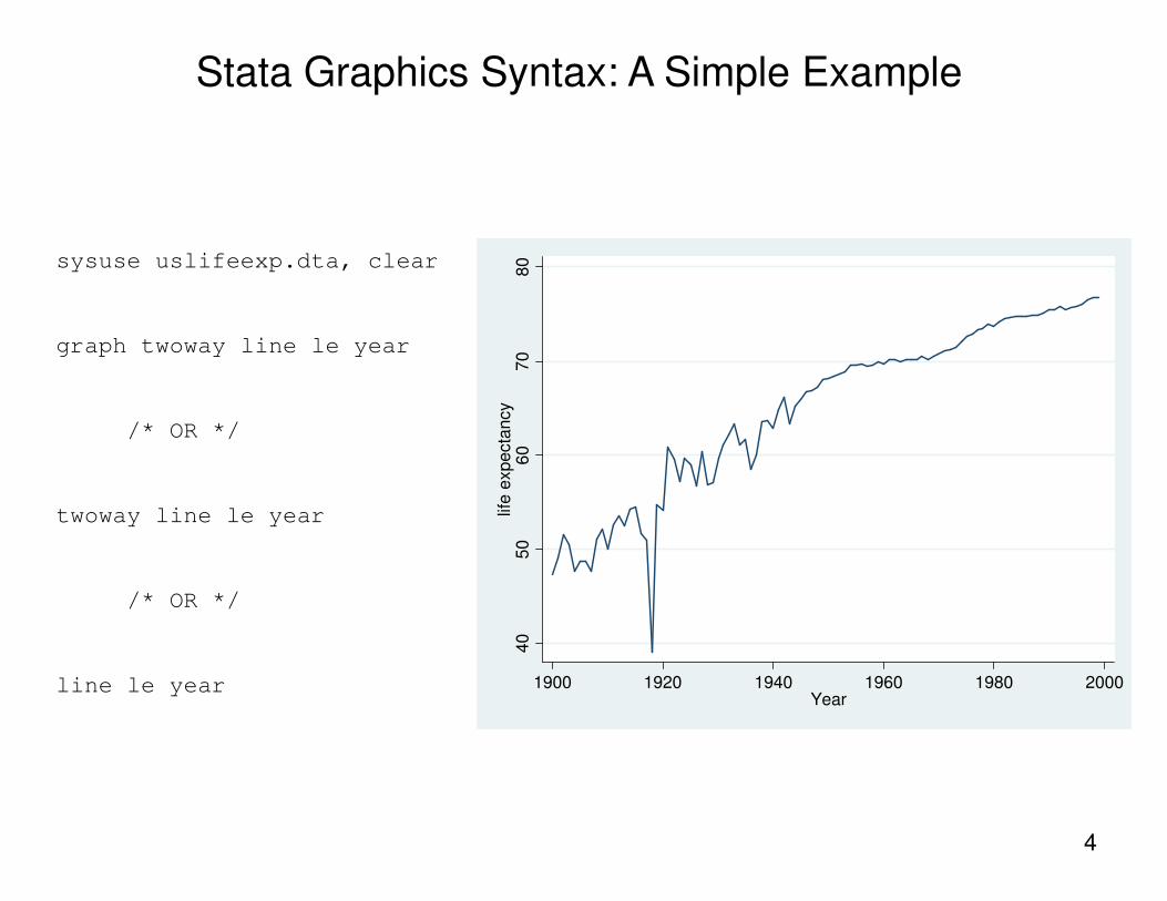
sysuse uslifeexp.dta, clear

graph twoway line le year

/* OR */

twoway line le year

/* OR */

line le year

40

50

60

70

80

life e

xpecta

ncy

1900 1920 1940 1960 1980 2000Year

Stata Graphics Syntax: A Simple Example

5

line le year, scheme(s1mono)

line le year, scheme(economist)

/* to see list of

scheme names:

graph query, schemes

to change default scheme:

set scheme schemename

*/

40

50

60

70

80

life e

xpecta

ncy

1900 1920 1940 1960 1980 2000Year

40

50

60

70

80

life e

xpecta

ncy

1900 1920 1940 1960 1980 2000Year

Using Schemes

6

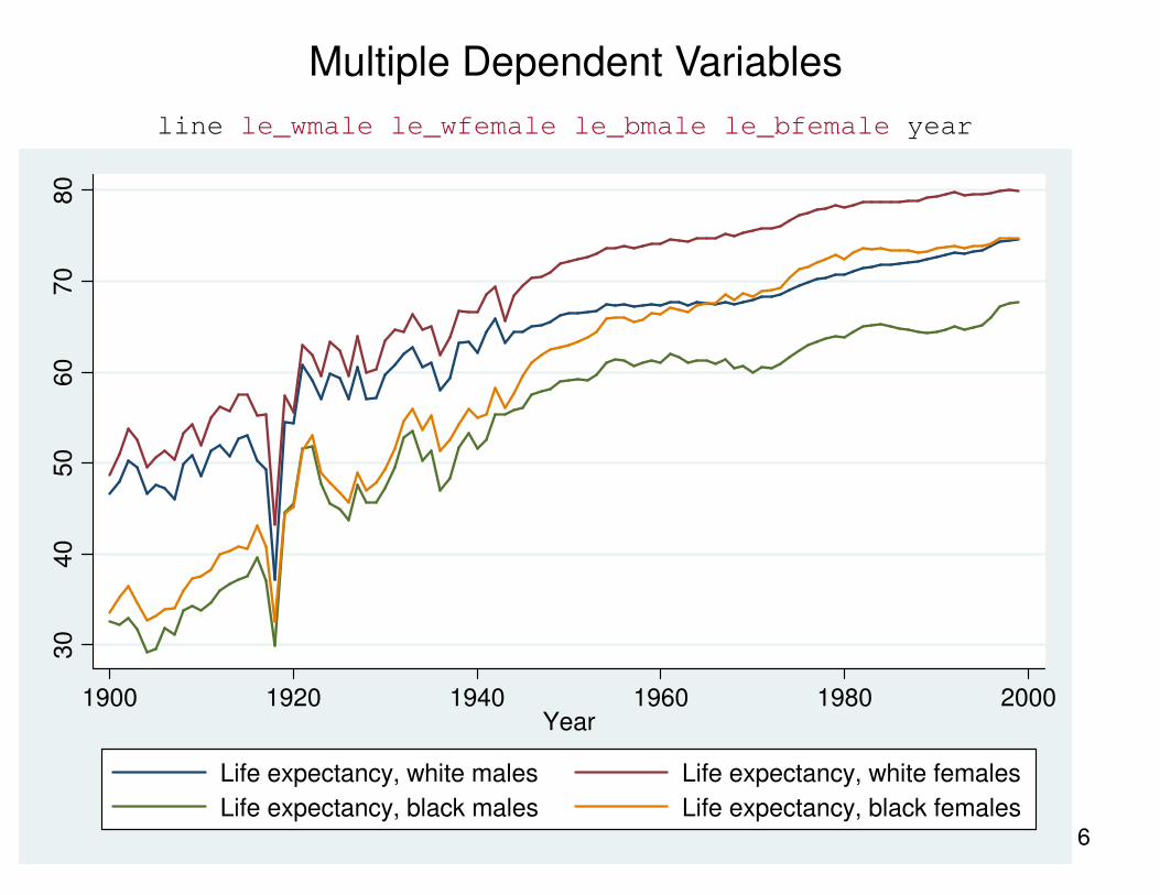
line le_wmale le_wfemale le_bmale le_bfemale year

30

40

50

60

70

80

1900 1920 1940 1960 1980 2000Year

Life expectancy, white males Life expectancy, white females

Life expectancy, black males Life expectancy, black females

Multiple Dependent Variables

7

Adding Text

line le_wmale le_wfemale le_bmale le_bfemale year ///

, text(32 1920 “{bf:1918} {it:Influenza} Pandemic", place(3))

1918 Influenza Pandemic

30

40

50

60

70

80

1900 1920 1940 1960 1980 2000Year

Life expectancy, white males Life expectancy, white females

Life expectancy, black males Life expectancy, black females

8

scatter ///

le year if year >= 1950 ///

|| lfit le year if year >= 1950

/* OR */

twoway ///

(scatter le year if year >= 1950) ///

(lfit le year if year >= 1950)

/* OR */

#delimit ;

twoway

(scatter le year if year >= 1950)

(lfit le year if year >= 1950);

#delimit cr

scatter le year if year >= 1950 || lfit le year if year >= 1950

/* OR */

Overlaying Two-Way Plot Types

68

70

72

74

76

1950 1960 1970 1980 1990 2000Year

life expectancy Fitted values

9

scatter le year if year >= 1925 ///

|| lfit le year if year >= 1925 & ///

year < 1950 ///

|| lfit le year if year >= 1950

/* OR */

twoway ///

(scatter le year if year >= 1925) ///

(lfit le year if year >= 1925 & ///

year < 1950) ///

(lfit le year if year >= 1950)

/* OR */

#delimit ;

scatter le year if year >= 1925

|| lfit le year if year >= 1925 & year < 1950

|| lfit le year if year >= 1950;

#delimit cr

55

60

65

70

75

1920 1940 1960 1980 2000Year

life expectancy Fitted values

Fitted values


10

#delimit ;

scatter le_male le_female year if year >= 1950

|| lfit le_male year if year >= 1950

|| lfit le_female year if year >= 1950;

#delimit cr

65

70

75

80

1950 1960 1970 1980 1990 2000Year

Life expectancy, males Life expectancy, females

Fitted values Fitted values


11

Adding a Title and Removing the Legend

#delimit ;

scatter le_male le_female year if year >= 1950

|| lfit le_male year if year >= 1950

|| lfit le_female year if year >= 1950

,title("US Male and Female Life Expectancy, 1950-2000")

text(75 1978 "Female", place(3))

text(68 1978 "Male", place(3))

legend(off);

#delimit cr

Female

Male

65

70

75

80

1950 1960 1970 1980 1990 2000Year

US Male and Female Life Expectancy, 1950-2000

12

50

60

70

80

Life e

xp

ecta

ncy a

t bir

th

20 40 60 80 100Percent of population with access to safe water

Linear fit 95% CI

Life expectancy at birth by access to safe water, 1998

sysuse lifeexp.dta, clear

#delimit ;

twoway

(lfitci lexp safewater if region == 2) /* North America */

(scatter lexp safewater if region == 2)

,title("Life expectancy at birth by access to safe water, 1998")

ytitle("Life expectancy at birth")

xtitle("Percent of population with access to safe water")

legend(ring(0) pos(5) order(2 "Linear fit" 1 "95% CI"));

#delimit cr

Showing Confidence Intervals, Labelling Axes, Modifying Legend

13

Canada

Cuba

Dominican Republic

El Salvador

Guatemala

Haiti

Honduras

Jamaica

Mexico

Nicaragua

Panama

Puerto Rico

Trinidad and Tobago

50

60

70

80

Life e

xp

ecta

ncy a

t bir

th


Linear fit 95% CI

North America


twoway


(scatter lexp safewater if region == 2, mlabel(country))


subtitle("North America")



legend(ring(0) pos(5) order(2 "Linear fit" 1 "95% CI"));

Markers Labels and Subtitles

14

Canada

Cuba

Dominican Republic

El Salvador

Guatemala

Haiti

Honduras

Jamaica

Mexico

Nicaragua

PanamaPuerto Rico

Trinidad and Tobago

50

60

70

80

Life e

xp

ecta

ncy a

t bir

th


Linear fit 95% CI

North America


generate pos = 12 if country == "Panama"

replace pos = 12 if country == "Honduras"

replace pos = 10 if country == "Cuba"

replace pos = 9 if country == "Jamaica"

replace pos = 9 if country == "El Salvador"

replace pos = 9 if country == "Trinidad and Tobago"

replace pos = 9 if country == "Dominican Republic"

#delimit ;

twoway


(scatter lexp safewater if region == 2

, mlabel(country) mlabvposition(pos))


subtitle("North America")



legend(ring(0) pos(5) order(2 "Linear fit" 1 "95% CI"))

plotregion(margin(r+10));

#delimit cr

Position of Marker Labels

15

Canada

Cuba

Dominican Republic

El Salvador

Guatemala

Haiti

Honduras

Jamaica

Mexico

Nicaragua

Panama

Puerto Rico

Trinidad and TobagoArgentina

Bolivia

Brazil

Chile

ColombiaEcuadorParaguayPeru

UruguayVenezuela

55

60

65

70

75

80

Life e

xp

ecta

ncy a

t bir

th


North and South America


#delimit ;

twoway

(scatter lexp safewater if region == 2 | region == 3

,mlabel(country))


subtitle("North and South America")



plotregion(margin(r+10));

#delimit cr

Position of Marker Labels

16

Canada

Cuba

Dominican Republic

El Salvador

Guatemala

Haiti

Honduras

Jamaica

Mexico

Nicaragua

Panama

Puerto Rico


Bolivia

Brazil

Chile


UruguayVenezuela

55

60

65

70

75

80

Life e

xp

ecta

ncy a

t bir

th


North America

South America



replace pos = 9 if country == "Argentina"

replace pos = 9 if country == "Canada"

replace pos = 9 if country == "Cuba"

replace pos = 9 if country == "Panama"

replace pos = 9 if country == "Venezuela"

replace pos = 9 if country == "Jamaica"

replace pos = 9 if country == "Dominican Republic"

replace pos = 9 if country == "Ecuador"

replace pos = 9 if country == "El Salvador"

replace pos = 12 if country == "Puerto Rico"

#delimit ;

twoway


,mlabel(country) mlabvposition(pos))


,mlabel(country) mlabvposition(pos))





legend(ring(0) pos(5) order(1 "North America" 2 "South America") cols(1));

#delimit cr

Position of Marker

Labels

and

Legend Display

17

Marker Size and Symbol, Line Color

Canada

Cuba

Dominican Republic

El Salvador

Guatemala

Haiti

Honduras

Jamaica

Mexico

Nicaragua

Panama

Puerto Rico


Bolivia

Brazil

Chile


UruguayVenezuela

55

60

65

70

75

80

Life e

xp

ecta

ncy a

t bir

th


North America

South America

North America linear fit

South America linear fit



twoway


,mlabel(country) mlabvposition(pos) msize(small))


,mlabel(country) mlabvposition(pos) msize(small) msymbol(circle_hollow))

(lfit lexp safewater if region == 2, clcolor(navy))

(lfit lexp safewater if region == 3, clcolor(maroon))





legend(ring(0) pos(5) cols(1) order(1 "North America" 2 "South America"

3 "North America linear fit" 4 "South America linear fit"));

18

Canada

Cuba

Dominican Republic

El Salvador

Guatemala

Haiti

Honduras

Jamaica

Mexico

Nicaragua

Panama

Puerto Rico


Bolivia

Brazil

Chile


UruguayVenezuela

55

60

65

70

75

80

Life e

xp

ecta

ncy a

t bir

th


North America

South America

North America linear fit

South America linear fit



twoway


,mlabel(country) mlabvposition(pos) msize(small) mcolor(black) mlabcolor(black))


,mlabel(country) mlabvposition(pos) msize(small) mcolor(black) mlabcolor(black)

msymbol(circle_hollow))

(lfit lexp safewater if region == 2, clcolor(black))

(lfit lexp safewater if region == 3, clcolor(black) clpattern(dash))

,title("Life expectancy at birth by access to safe water, 1998", color(black))




legend(ring(0) pos(5) cols(1) order(1 "North America" 2 "South America"

3 "North America linear fit" 4 "South America linear fit"));

Marker and Marker Label Color, Line Style

19

50

60

70

80

50

60

70

80

20 40 60 80 100 20 40 60 80 100

Eur & C.Asia N.A.

S.A. Total

Life

exp

ecta

ncy a

t b

irth

Percent of population with access to safe waterGraphs by Region

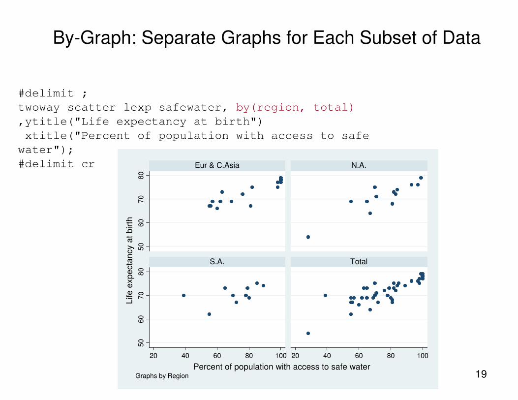
#delimit ;

twoway scatter lexp safewater, by(region, total)

,ytitle("Life expectancy at birth")

xtitle("Percent of population with access to safe

water");

#delimit cr

By-Graph: Separate Graphs for Each Subset of Data

20

50

60

70

80

50

60

70

80

20 40 60 80 10020 40 60 80 100

Eur & C.Asia N.A.

S.A. Total

Life

exp

ecta

ncy a

t b

irth

Percent of population with access to safe water

Life expectancy by access to safe water

twoway scatter lexp safewater

,by(region,total style(compact)

title("Life expectancy by access to safe water") note(""))


xtitle("Percent of population with access to safe water");

By-Graph Options

21

55

60

65

70

75

80

55

60

65

70

75

80

30 40 50 60 70 80 90 100 30 40 50 60 70 80 90 100

Eur & C.Asia N.A.

S.A. Total

Life

exp

ecta

ncy a

t b

irth

Percent of population with access to safe water


twoway scatter lexp safewater

, by(region,total style(compact)

title("Life expectancy by access to safe water") note(""))

xscale(range(20 100))

xtick(20(10)100)

xlabel(30(10)100, labsize(small))



ylabel(55(5)80, angle(0));

Axis Scale, Ticks and Labels

22

Canada

Cuba

Dominican Republic

El Salvador

Guatemala

Haiti

Honduras

Jamaica

Mexico

Nicaragua

Panama

Puerto Rico

Trinidad and Tobago

55

60

65

70

75

80

Life e

xp

ecta

ncy a

t bir

th


North America

twoway

(scatter lexp safewater if region == 2,

mcolor(black) msize(small)

mlabel(country) mlabvposition(pos) mlabcolor(black))


,name(north_america, replace)

subtitle("North America", color(black))

ylabel(,angle(0))



legend(off);

Storing Graphs in Memory

23

Argentina

Bolivia

Brazil

Chile

ColombiaEcuadorParaguay

Peru

Uruguay

Venezuela

60

65

70

75

Life e

xp

ecta

ncy a

t bir

th

40 50 60 70 80 90Percent of population with access to safe water

South America

twoway

(scatter lexp_sa safewater if region == 3,

mcolor(black) msize(small)

mlabel(country) mlabvposition(pos) mlabcolor(black))


,name(south_america, replace)

subtitle("South America", color(black))

ylabel(, angle(0))



legend(off);

Storing Graphs in Memory

24

Canada

Cuba

Dominican RepublicEl Salvador

Guatemala

Haiti

Honduras

Jamaica

Mexico

Nicaragua

Panama

Puerto Rico

Trinidad and Tobago

55

60

65

70

75

80

Life e

xpecta

ncy a

t bir

th


North America

Argentina

Bolivia

Brazil

Chile


UruguayVenezuela

60

65

70

75

Life e

xpecta

ncy a

t bir

th

40 50 60 70 80 90Percent of population with access to safe water

South America


graph combine north_america south_america

,title("Life expectancy by access to safe water", color(black)) col(1);

Combining Graphs

25

Canada

Cuba

Dominican Republic

El Salvador

Guatemala

Haiti

Honduras

Jamaica

Mexico

Nicaragua

Panama

Puerto Rico

Trinidad and Tobago

55

60

65

70

75

80

Life e

xpecta

ncy a

t birth


North America

Argentina

Bolivia

Brazil

Chile


UruguayVenezuela

55

60

65

70

75

80

Life e

xpecta

ncy a

t birth


South America


graph combine north_america south_america

,title

("Life expectancy by access to safe water",

color(black))

xcommon ycommon

xsize(7) ysize(10.5)

col(1);

Combining

Graphs

26

save graph in portable format (format determined by filename extension)

vector formats contain drawing instructions (.wmf .emf .ps .eps .pdf)

resolution independent

work well if graph my be resized

graph export north_america.wmf

raster formats save graph pixel-by-pixel (.png)

use current resolution

work well if including graph on web pages

graph export north_america.png

include "portable-format-graph" in Windows application (Word, Powerpoint):

Insert -> Picture -> From File

Saving and Including Stata Graphs

27

* Functions available starting with Stata 13

Using Mata Functions to Add Graphs to Word Document*

mata:

dh = _docx_new()

_docx_image_add(dh, “us_lifeexp_overall.emf”)

_docx_image_add(dh, “us_lifeexp_race_gender.emf”)

rc = _docx_save(dh, “us_lifeexp_graphs.docx”)

end

sysuse uslifeexp

line le year

graph export us_lifeexp_overall.emf, replace

line le_wmale le_wfemale le_bmale le_bfemale year

graph export us_lifeexp_race_gender.emf, replace

create Stata graphs and and use graph export to save graphs in portable format

use Mata functions to:

create Word document

add Stata graphs

save Word document

dawn koffman princeton university - office of … 14 graphics manual (may want to start with...

Documents