day 1 introduction to the basic heterogeneous … 1 introduction to the basic heterogeneous-agents...
TRANSCRIPT

Day 1
Introduction to the Basic Heterogeneous-AgentsIncomplete-Markets Model
Gianluca Violante
New York University
Mini-Course on “Policy in Models with Heterogeneous Agents”
Bank of Portugal, June 15-19, 2105
p. 1 /57

Motivation
• We are interested in building a class of models whose equilibriafeature a nontrivial endogenous distribution of income and wealthacross agents in order to address positive and normative policyquestions, such as:
1. What are the redistributive and welfare effects of changes inthe income tax code?
2. How is the size of fiscal multipliers affected by householdheterogeneity?
3. What is the optimal degree of tax progressivity? Or theoptimal quantity of government debt?
4. Does monetary policy have significant effects on the incomeand wealth distribution? Through which channels?
5. Are the macro effects of fiscal and monetary policy affected bythe presence of nontrivial heterogeneity?
p. 2 /57

Building blocks of the workhorse model
• Neoclassical growth model with idiosyncratic uninsurable risk
• The model is constructed around three building blocks:
1. the income-fluctuation problem
2. the neoclassical aggregate production function
3. the equilibrium of the asset market.
• We focus on the stationary equilibrium, for now, i.e., an economywithout aggregate shocks.
p. 3 /57

Block 1: Income fluctuation problem
• Individuals are subject to exogenous income shocks. Theseshocks are not fully insurable because of the lack of a completeset of Arrow-Debreu contingent claims.
• There is only a risk-free asset (i.e., and asset with non-statecontingent rate of return) in which the individual can save/borrow,and that the individual faces a borrowing (liquidity) constraint.
• A continuum of such agents subject to different shocks will giverise to a wealth distribution.
• Integrating wealth holdings across all agents will give rise to anaggregate supply of capital.
p. 4 /57

Blocks 2 and 3
• Aggregate production function: profit maximization of thecompetitive representative firm operating a CRS technology willgive rise to an aggregate demand for capital.
• Equilibrium in the asset market: Demand and supply interact inan asset market, an equilibrium interest rate arises endogenously.
If a full set of Arrow-Debreu contingent claims were available,the economy would collapse to a representative agent modelwith a stationary amount of savings such that Rβ = 1.
With uninsurable risk, the supply of savings is larger (R islower) because of precautionary saving, and consequentlyRβ < 1.
We like this result: this is a necessary condition for theincome-fluctuation problem to have a bounded consumptionsequence as solution.
p. 5 /57

Economy
• Demographics: the economy is populated with a continuum ofmeasure one of infinitely lived, ex-ante identical agents.
• Preferences: the individual has time-separable preferences overstreams of consumption
U(c0, c1, c2, ...) = E0
∞∑
t=0
βtu(ct),
• Endowment: each individual has a stochastic endowment ofefficiency units of labor εt ∈ E. The shocks obey the conditionalcdf π(dε, ε) = Pr (εt+1 ∈ dε | εt = ε) .
• Shocks are iid across individuals. A law of large numbers holds,so that π(dε, ε) is also the fraction of agents in the populationsubject to this particular transition.
p. 6 /57

Economy
• There is a unique invariant distribution Π∗ (dε) . As a result, theaggregate endowment of efficiency units
Ht =
∫
E
εΠ∗ (dε) , for all t
is constant over time and exogenously determined.
• Budget constraint: At time t, the budget constraint reads
ct + at+1 = Rtat + wtεt,
where ct is consumption, at+1 is next period wealth, Rt ≡ (1 + rt)is the gross interest rate and wt is the wage rate
• Wealth is held in the form of a one-period risk-free (or nonstate-contingent) bond whose return, next period is 1 + rt+1
p. 7 /57

Economy
• Liquidity constraint: At every t, agents face the borrowing limit
at+1 ≥ −b
where b is exogenously specified. Alternatively, we could assumeagents face the natural borrowing constraint, which is the DPV ofthe lowest possible realization of earnings
• Technology: The representative competitive firm produces withCRS production function Yt = F (Kt, Ht). Physical capitaldepreciates geometrically at rate δ ∈ (0, 1) .
• Market structure: final good market, labor market, and capitalmarket are all competitive.
• Aggregate resource constraint:
F (Kt, Ht) = Ct + It = Ct +Kt+1 − (1− δ)Kt
p. 8 /57

Mathematical preliminaries
• Individual states: (a, ε)
• Let λ be the distribution of agents over states. We would like thisobject to be a probability measure, so we need to define anappropriate mathematical structure.
• a: maximum asset holding in the economy, and for now assumethat such upper bound exists.
• Define the compact set A ≡ [−b, a] of possible asset holdings
• Let the the state space S be the Cartesian product A× E, and letBs be the Borel sigma-algebra over S. The space (S,Bs) is then ameasurable space.
• Let S =(A× E) be typical subset of Bs. For any element of thesigma algebra S ∈Bs, λ(S) is the measure of agents in the set S.
p. 9 /57

Mathematical preliminaries
• How can we characterize the way individuals transit across statesover time? I.e. how do we obtain next period distribution, giventhis period distribution? We need a transition function.
• Define Q ((a, ε) ,A× E) as the probability that an individual withcurrent state (a, ε) transits to the set A× E next period, formallyQ : S ×Bs → [0, 1], and
Q ((a, ε) ,A× E) = Ia′(a,ε)∈A
∫
E
π(dε′, ε)
where I· is the indicator function, and a′(a, ε) is saving policy
• Then Q is our transition function and the law of motion for thedistribution becomes:
λn+1 (A× E) =
∫
A×E
Q ((a, ε) ,A× E) dλn.
p. 10 /57

Mathematical preliminaries
• Let us now re-state the problem of the individual in recursive form:
v(a, ε;λ) = maxc,a′
u(c) + β
∫
E
v(a′, ε′;λ)π(dε′, ε) (1)
s.t.
c+ a′ = R (λ) a+ w (λ) ε
a′ ≥ −b
where, for clarity, we have made explicit the dependence of valuesprices from the distribution of agents.
• Strictly speaking this dependence is redundant in a stationaryenvironment and it can be omitted, since the probability measureλ is constant in equilibrium.
p. 11 /57

Stationary recursive competitive equilibrium
A stationary RCE is: a value function v : S → R; policy functions for thehousehold a′ : S → R, and c : S → R+; firm’s choices H and K; pricesr and w; and, a stationary measure λ∗ such that:
• given prices r and w, the policy functions a′ and c solve thehousehold’s problem and v is the associated value function
• given r and w, the firm chooses optimally its capital K and itslabor H, i.e., r + δ = FK(K,H) and w = FH(K,H)
• the labor market clears: H =∫
A×Eεdλ∗
• the asset market clears: K =∫
A×Eadλ∗,
• the goods market clears:∫
A×Ec(a, ε)dλ∗ + δK = F (K,H),
p. 12 /57

Stationary recursive competitive equilibrium
• for all (A× E) ∈ Σs, the invariant probability measure λ∗ satisfies
λ∗ (A× E) =
∫
A×E
Q ((a, ε) ,A× E) dλ∗,
where Q is the transition function defined earlier:
Q ((a, ε) ,A× E) = Ia′(a,ε)∈A
∫
E
π(dε′, ε)
p. 13 /57

Existence of the stationary equilibrium
• Existence boils down, like in every GE model, to show that theexcess demand function (i.e., a function of the price) in eachmarket is continuous, and intersects zero.
• Equilibrium in the labor market is trivial: aggregate labor supply isexogenous and labor demand is strictly decreasing in wages.
• By Walras law, if we prove that the equilibrium in the asset marketexists and is unique, we are done.
• Demand for capital: From the optimal choice of the firm:
K(r) = F−1k (r + δ)
Note that for r = −δ, K → +∞, while for r → +∞, K → 0. Thus,the demand of capital is a continuous, strictly decreasing functionof the interest rate r.
p. 14 /57

SS Equilibrium in the Aiyagari model
p. 15 /57

Existence of the Stationary Equilibrium
• Supply of capital: Need to show that aggregate supply function
A(r) =
∫
A×E
adλ∗r
is continuous in r and crosses the aggregate demand function.
• If r = 1β− 1, then we know by the super-martingale converge
theorem that the aggregate supply of assets goes to infinity, i.e.
A(
1β− 1
)
→ ∞
• If r = −1 the individual would like to borrow until the limit, as everyunit of capital saved will vanish, so A(−1) → −b.
• Thus, if A (r) is continuous, it will cross the aggregate demandand we would have an existence result.
p. 16 /57
Existence of the stationary equilibrium
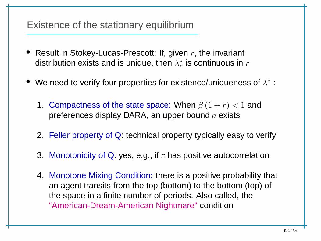
• Result in Stokey-Lucas-Prescott: If, given r, the invariantdistribution exists and is unique, then λ∗
r is continuous in r
• We need to verify four properties for existence/uniqueness of λ∗ :
1. Compactness of the state space: When β (1 + r) < 1 andpreferences display DARA, an upper bound a exists
2. Feller property of Q: technical property typically easy to verify
3. Monotonicity of Q: yes, e.g., if ε has positive autocorrelation
4. Monotone Mixing Condition: there is a positive probability thatan agent transits from the top (bottom) to the bottom (top) ofthe space in a finite number of periods. Also called, the“American-Dream-American Nightmare" condition
p. 17 /57

Uniqueness of the stationary equilibrium
• If, in addition, we could show that A (r) is strictly increasing, wewould prove uniqueness.
• Unfortunately, there are no results on the monotonicity of theaggregate supply of capital with respect to r, so uniqueness isnever guaranteed.
• A higher r has both income and substitution effects on savings:the relative importances between the two could switch at a certainlevel of assets, so it is very hard to assess what a change in rdoes to the distribution of assets.
p. 18 /57

SS Equilibrium in the Aiyagari model
p. 19 /57

Some aspects of the calibration
• Discount rate: The discount rate βshould be chosen to matchthe aggregate wealth-income ratio for the U.S. economy which isaround 3− 4 depending whether we include residential capital.
It requires an internal calibration: must solve for theequilibrium for each values of β and try to hit the K/Y target.Use the complete-markets β as a guidance, e.g. with CDtechnology:
β =1
1 + α(
YK
)
− δ=
1
1 + 0.33 (0.33)− 0.06= 0.951.
Labor income process: Need to estimate error componentmodel from micro data on individual income dynamics.
Borrowing constraint: Calibrate the borrowing constraint inorder to match, say, the fraction of agents with negative net worthwhich is around 10% in the U.S. economy.
p. 20 /57

Wealth inequality at the top
• Standard model does not generate enough wealth at the top:model Gini is 0.6, data Gini is 0.8.
Heterogeneity in discount factors: patients agents (richer)save more (Krusell and Smith, 1997)
Stronger bequest motive for the rich: rich save more tobequeath (De Nardi, 2003)
Extraordinary but transitory income realization: rich save morefor precautionary reasons (Castaneda et al, 2003)
Stochastic rate of return (Benhabib et al., 2014)
Entrepreneurs with projects yielding higher, but stochastic,rate of return than r (Quadrini, 2000)
• New question: do these models get wealth mobility right?p. 21 /57

Trade-off between efficiency and social insurance
• Since earnings risk is uninsurable because of marketincompleteness, there is scope for public insurance, i.e.government intervention through taxation and redistribution fromthe rich-lucky to the poor-unlucky
• Ramsey problem: the government chooses a labor income tax τand a lump-sum subsidy T in order to maximize the ex-antewelfare of the a newborn in SS (progressive tax/transfer scheme)
• With exogenous labor supply, the optimal tax rate in the Aiyagarieconomy would be τ = 1.
• A more interesting economy is one with an endogenous margin oflabor/leisure choice where there is a trade-off between insuranceand efficiency.
p. 22 /57

Aiyagari model with labor supply
• Period utility is given by u(c, l) i.e., we introduce leisure l ∈ (0, 1)in order to have a margin where distortions matter. L
• We will have an optimal policy for labor supply h(a, ε). Agentsmight be using their elastic labor supply to self-insure.
• Take an agent who is borrowing constrained and has a lowrealization of the productivity shock. To keep his consumptionhigh, she could intensify his labor supply
this introduces a bias in the estimation of the Frisch elasticity
• The new budget constraint reads:
c+ a′ = (1 + r) a+ (1− τ)wεh+ T,
p. 23 /57

Aiyagari model with labor supply
• The new equilibrium condition in the labor market becomes
N =
∫
A×E
εh(a, ε)dλ∗
where LHS is aggregate labor demand and the RHS is aggregatelabor supply
• The government budget constraint (balanced in equilibrium) reads
T = τwN,
• Stationary RCE similar, plus decision rule for hours worked andgovernment budget constraint
• What level of government redistribution maximizes welfare?
p. 24 /57

Answer
• In an economy with heterogeneous agents there is not a uniquewelfare function, it all depends on what weights are assigned toeach type. Assume a utilitarian social welfare function:
maxτ
W (τ) =
∫
A×E
v∗(a, ε; τ)dλ∗τ ,
where v∗(a, ε; τ) is the value function associated to thecompetitive equilibrium indexed by τ.
• Need to solve the stationary equilibrium for a range of differentvalues on τ ∈ (0, 1) .
• For very low τ , welfare is low because agents have too muchundesired consumption fluctuations. For very high τ , consumptioninsurance is very high but heavy distortions on labor supply areimposed. There will be an interior level of τ , call it τ∗, thatmaximizes social welfare
p. 25 /57

Optimal quantity of government debt
• Same economy as before, plus...
• ... government debt: an additional risk-free asset and, by noarbitrage, it must carry the same rate of return as capital inequilibrium.
• Government has two type of outlays: lump-sum transfers T , andinterest payments on the stock of public (one-period) debt B.Outlays financed by distortionary taxes on labor income at rate τ.
• In steady-state the government budget constraint reads
T +RB = B′ + τwH,
The equilibrium condition in the asset market is now:
K (r) +B = A (r) ⇒ K (r) = A (r)−B.
p. 26 /57

Pros and cons of government debt
• Cons:
Debt is costly because financing interest payments on debtrequires distortionary taxes.
Debt crowds-out productive capital because some of thesavings are shifted away from productive capital intounproductive debt.
• Pros:
The interest rate rises unambiguously, which reduces the costof holding assets for self-insurance (liquidity effect of debt)
But with a natural borrowing limit, the rise in r would tightenthe constraint
p. 27 /57

Unconstrained efficiency in the Aiyagari model
• Equilibrium of the neoclassical growth model with idiosyncraticrisk displays over-accumulation of capital relative to the first bestwhere Rβ = 1.
• Given the lack of perfect insurance markets, agents save more forself-insurance, the capital stock goes up, the interest rate fallsbelow the discount rate, i.e. Rβ < 1.
• Incomplete-markets equilibrium allocations are Pareto inefficient,or, not first-best.
• An unconstrained planner can achieve Pareto efficiency becauseit has more freedom in allocating resources than it is provided bythe system of incomplete markets: it can make state-contingenttransfers across agents.
p. 28 /57

Constrained efficiency in the Aiyagari model
• We assume that the planner cannot overcome directly the frictionsimposed by the missing markets, i.e., it faces the same constraintson trade and transfer of resources across agents as in the originalenvironment. This is the concept of constrained efficiency.
• We must solve the problem of a planner that instructsconsumption and saving decisions to each agent —by choosing aconsumption policy function— while facing the same technologyand asset structure (i.e., only a risk-free bond), and hence thesame set of constraints, that agents face in the decentralizedequilibrium.
• We will find that the competitive equilibrium is constrainedinefficient because of a “pecuniary externality”: by choosing aconsumption policy for each agent in the economy, the plannercan affect prices in order to redistribute in the right way.
p. 29 /57

Constrained efficiency in the Aiyagari model
• The planner who maximizes social welfare by choosing a savingpolicy g (a, ε) (i.e., a saving level a′ for every point in the statespace) solves:
Ω (λ) = maxg(a,ε)∈A
∫
A×E
u [R (λ) a+ w (λ) ε− g (a, ε)] dλ+ βΩ (λ′)
s.t.
R (λ) = FK (K,H) and w (λ) = FH (K,H)
H =
∫
A×E
εdλ
K =
∫
A×E
adλ
λ′ (A× E) =
∫
A×E
1g(a,ε)∈Aπ (ε′ ∈ E , ε) dλ (a, ε)
p. 30 /57

Constrained efficiency in the Aiyagari model
• In the stationary competitive equilibrium, the FOC of the agent is:
uc ≥ βR (λ∗)∑
ε′∈E
u′cπ (ε′, ε)
• The FOC for the planner who chooses the level a′ for a particularpair (a, ε) is:
uc ≥ βR (λ′)∑
ε′∈E
u′cπ (ε′, ε)+β
∫
A×E
(a′F ′KK + ε′F ′
HK)u′cdλ
′
• Extra term: planner internalizes effects that individual savingshave on prices, so it “takes derivatives” also with respect to prices= marginal productivities of the factors of production
• Extra term can be either positive or negative: in the representativeagent case, this term is zero because F is CRS
p. 31 /57

Constrained efficiency in the Aiyagari model
• We can use the CRS assumption on F and rewrite:
uc ≥ βR (λ′)∑
ε′∈E
u′cπ (ε′, ε)+βF ′
KKK′
∫
A×E
(
a′
K′−
ε′
H
)
u′cdλ
′.
• Factor composition of income of poor agents (those with weight u′c
large) determines the sign of extra term
• If their income is labor-intensive, then the extra term will bepositive since F ′
KK < 0 and, a′
K′< ε′
H.
• The planner wants agents to save more than in the decentralizedequilibrium: under-accumulation relative to constrained optimum
• If the poor have mostly labor income, then the way to redistributefrom rich to poor is to increase equilibrium wages by inducingagents to save more than in equilibrium.
p. 32 /57

NUMERICAL SOLUTION
p. 33 /57

Policy function iteration with linear interpolation
1. Construct a grid on the asset space a0, a2, ..., am witha0 = a = 0.
2. Guess an initial vector of decision rules for a′′ on the grid points,call it a0 (ai, yj).
3. For each point (ai, yj) on the grid, check whether the borrowingconstraint binds. I.e. check whether:
uc (Rai + yj − a0)−βR∑
y′∈Y
π (y′|yj)uc (Ra0 + y′ − a0 (a0, y′)) > 0.
4. If this inequality holds, the borrowing constraint binds. Then, seta0 (ai, yj) = a0 and repeat this check for the next grid point. If theequation instead holds with the < inequality, we have an interiorsolution (it is optimal to save for the household) and we proceedto the next step.
p. 34 /57

Policy function iteration with linear interpolation
5. For each point (ai, yj) on the grid, use a nonlinear equation solverto find the solution a∗ of the nonlinear equation
uc (Rai + yj − a∗)− βR∑
y′∈Y
π (y′|yj)uc (Ra∗ + y′ − a0 (a∗, y′)) = 0
(a) Need to evaluate the function a0 (a, y′) outside grid points:
assume it is piecewise linear.
(b) Every time the solver calls an a∗ which lies between gridpoints, do as follows. First, find the pair of adjacent grid pointsai, ai+1 such that ai < a∗ < ai+1, and then compute
a0 (a∗, y′) = a0 (ai, y
′)+(a∗ − ai)
(
a0 (ai+1, y′)− a0 (ai, y
′)
ai+1 − ai
)
(c) If the solution of the nonlinear equation is a∗, then seta′0 (ai, yj) = a∗ and iterate on the next grid point.
p. 35 /57

Policy function iteration with linear interpolation
6. Check convergence by comparing a′0 (ai, yj)− a0 (ai, yj) throughsome pre-specified norm. For example, declare convergence atiteration n when
maxi,j
|a′n (ai, yj)− an (ai, yj) | < ε
for some small number ε which determines the degree oftolerance in the solution algorithm.
7. If convergence is achieved, stop. Otherwise, go back to point 3with the new guess a1 (ai, yj) = a′0 (ai, yj).
Note that the most time-consuming step in this procedure is 5, theroot-finding problem. We now discuss how to avoid it.
p. 36 /57

Endogenous grid method (EGM)
• EGM is much faster than the traditional method because it doesnot require the use of a nonlinear equation solver
• The essential idea of the method is to construct a grid on a′, nextperiod’s asset holdings, rather than on a, as is done in thestandard algorithm.
• The method also requires the policy function to be at least weaklymonotonic in the state
• Recall the Euler equation:
uc (c (a, y)) ≥ βR∑
y′∈Y
π (y′|y)uc (c (a′, y′)) .
• We start from a guess c0 (a, y) and iterate on the Euler Equationuntil the decision rule for consumption that we solve for isessentially identical to the one in the previous iteration.
p. 37 /57

EGM: Algorithm
1. Construct a grid for (a, y)
2. Guess a policy function c0 (ai, yj). If y is persistent, a good initialguess is to set c0 (ai, yj) = rai + yj which is the solution underquadratic utility if income follows a random walk.
3. Fix yj . Instead of iterating over ai , we iterate over a′i. For anypair a′i, yj on the mesh construct the RHS of the Euler equation[call it B (a′i, yj)]
B (a′i, yj) ≡ βR∑
y′∈Y
π (y′|yj)uc (c0 (a′i, y
′))
where the RHS of this equation uses the guess c0.
p. 38 /57

EGM: Algorithm
4. Use the Euler equation to solve for the value c (a′i, yj) that satisfies
uc (c (a′i, yj)) = B (a′i, yj)
and note that it can be done analytically, e.g. for uc (c) = c−γ we
have c (a′i, yj) = [B (a′i, yj)]− 1
γ . Here algorithm becomes muchmore efficient because it does not require a nonlinear solver.
5. From the budget constraint:
c (a′i, yj) + a′i = Ra∗i + yj
solve for a∗ (a′i, yj) the value of assets today that would lead theconsumer to have a′i assets tomorrow if her income shock was yjtoday. This yields c (a∗i , yj) = c (a′i, yj), a function not defined onthe grid points. This is the endogenous grid and it changes oneach iteration.
p. 39 /57

EGM: Algorithm
6. Let a∗0 be the value of asset holdings that induces the borrowingconstraint to bind next period, i.e., the value for a∗ that solves thatequation at the point a′0, the lower bound of the grid.
7. Now we need to update our guess defined on the original grid.
• To get new guess c1 (ai, yj) on grid points ai > a∗0 we can usesimple linear interpolation methods using values for
c (a∗n, yj) , c(
a∗n+1, yj)
on the two most adjacent values
a∗n, a∗n+1
that bracket ai.
• If some points ai are beyond a∗m, the upper bound of theendogenous grid, just extend linearly the function
p. 40 /57

EGM: Algorithm
• To update the consumption policy function on grid valuesai < a∗0, we use the budget constraint:
c1 (ai, yj) = Rai + yj − a0
since we cannot use the Euler equation as the borrowingconstraint is binding for sure next period: the reason is that wefound it was binding at a∗0, therefore a fortiori it will be bindingfor ai < a∗0.
8. Check convergence as before.
p. 41 /57

SS Equilibrium of the Aiyagari model
Fixed point algorithm over the interest rate (or K).
1. Fix an initial guess for the interest rate r0 ∈(
−δ, 1β− 1
)
. r0 is our
first candidate for the equilibrium (the superscript denotes theiteration number).
2. Given r0, solve the dynamic programming problem of the agent toobtain a′ = g(a, y; r0). We described several solution methods.
3. Given the decision rule for assets next period g(a, y; r0) and theMarkov transition over productivity shocks Γ (y′, y), we canconstruct the transition function Q
(
r0)
and, by successiveiterations, we obtain the fixed point distribution Λ
(
r0)
, conditionalon the candidate interest rate r0 [details later]
p. 42 /57

SS Equilibrium of the Aiyagari model
4. Compute the aggregate demand of capital K(
r0)
from theoptimal choice of the firm who takes r0 as given, i.e.
K(r0) = F−1k (r0 + δ)
5. Compute the integral:
A(
r0)
=
∫
A×Y
g(a, y; r0)dΛ(a, y; r0)
which gives the aggregate supply of assets. This can be easilydone by using the invariant distribution obtained in step 3.
p. 43 /57

SS Equilibrium of the Aiyagari model
6. Compare K(
r0)
with A(
r0)
to verify whether the asset marketclearing condition holds.
7. Update your guess for the interest rate from r0 to r1 and go backto step 1.
8. Keep iterating until you reach convergence of the interest rate,i.e., until, at iteration n:
|rn+1 − rn| < ε
p. 44 /57

Speed vs stability of the algorithm
• Two tricks that make the algorithm a lot more stable, albeit slower
1. Don’t use gradient methods to solve for r∗ in the outer loop.Use bisection. Given r0, to obtain the new candidate r1 bisectbetween r0 and
[
FK(A(
r0)
)− δ]
r1 =1
2
r0 +[
FK(A(
r0)
)− δ]
which are, by construction, on opposite sides of thesteady-state interest rate r∗. Even better, use “dampening” inupdating:
r1 = ωr0 + (1− ω)[
FK(A(
r0)
)− δ]
with weight ω = 0.8− 0.9 for example.
p. 45 /57

Speed vs stability of the algorithm
2. When you resolve the household problem for a new value of theinterest rate rn+1, do not initialize the decision rule from the onecorresponding to rn obtained in the previous loop. Always startfrom the same guess of the decision rule to avoid propagationerror in wealth distribution. Slower, but safer.
p. 46 /57

Calculating the invariant distribution
• Continuum of households makes the wealth distribution acontinuous function and therefore an infinite-dimensional object inthe state space. Need approximation.
• Small errors in computing the invariant distribution, particularly inmodels with aggregate shocks, can accumulate and lead tosignificant errors in the equilibrium values of aggregate variables.
• Three approaches:
1. discretization of the invariant density function
2. eigenvector method
3. simulation of an artificial panel
p. 47 /57

Discretization of the invariant density function
• A common approach involves finding an approximation to theinvariant density function λ (a, y)
• We will approximate the density by a probability distributionfunction defined over a discretized version of the state space. Thegrid should be finer than the one used to compute the optimalsavings rule.
• Choose initial density functions λ0 (ak, yi) . For example
λ0 (ak, yi) =
0 if k > 1 and i > 1
1 if k = 1 and i = 1
i.e., all the mass is at the borrowing limit and at the lowestrealization of the income shock
p. 48 /57

Discretization of the invariant density function
• For every (ak, yj) on the grid:
λ1 (ak, yj) =∑
yi∈Y
Γij
∑
m∈Mi
ak+1 − g (am, yi)
ak+1 − akλ0 (am, yi)
λ1 (ak+1, yj) =∑
yi∈Y
Γij
∑
m∈Mi
g (am, yi)− akak+1 − ak
λ0 (am, yi)
where
Mi = m : ak ≤ g (am, yi) ≤ ak+1
p. 49 /57
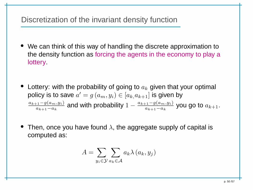
Discretization of the invariant density function
• We can think of this way of handling the discrete approximation tothe density function as forcing the agents in the economy to play alottery.
• Lottery: with the probability of going to ak given that your optimalpolicy is to save a′ = g (am, yi) ∈ [ak,ak+1] is given byak+1−g(am,yi)
ak+1−akand with probability 1− ak+1−g(am,yi)
ak+1−akyou go to ak+1.
• Then, once you have found λ, the aggregate supply of capital iscomputed as:
A =∑
yi∈Y
∑
ak∈A
akλ (ak, yj)
p. 50 /57

Eigenvector method
• Let A be a square matrix. If there is a vector v 6= 0 in Rn such that:
vA = ev
for some scalar e, then e is called the eigenvalue of A withcorresponding (left) eigenvector v.
• Recall that the definition of invariant pdf for a Markov transitionmatrix Q is λ∗ that satisfies:
λ∗Q = λ∗
thus an invariant distribution is the eigenvector of the matrix Qassociated to eigenvalue 1.
• How do we guarantee this eigenvector is unique and how do wefind it in that case?
p. 51 /57

Eigenvector method
• Perron-Frobenius Theorem: Let Q be a transition matrix of anhomogeneous ergodic Markov chain. Then Q has a uniquedominant eigenvalue e = 1 such that:
its associated eigenvector has all positive entries
all other eigenvalues are smaller than e in absolute value
Q has no other eigenvector with all non-negative entries
• This eigenvector (renormalized so that it sums to one) is theunique invariant distribution
p. 52 /57

Eigenvector methods
• How do we construct Q?
• Let Q (a′, y′; a, y) be the JN × JN transition matrix from state(a, y) into (a′, y′) . Since the evolution of y′ is independent of a:
Q (a′, y′; a, y) = Qa (a′; a, y)⊗ Γ (y′, y)
where, if a′ = g (a, y) is such that ak+1 ≤ a′ < ak, then we define:
Qa (ak; a, y) =ak+1 − g (a, y)
ak+1 − ak
Qa (ak+1; a, y) =g (a, y)− akak+1 − ak
... same lottery we used before for the density
p. 53 /57

Eigenvector methods
• In practice: the Q function is very large and very sparse and thereare many eigenvalues very close to one
• The corresponding eigenvectors generally have negativecomponents that are inappropriate for the density function.
• Idea: perturb the zero entries of Q by adding a perturbationconstant η and renormalizing the rows of Q.
• Then find the unique non-negative eigenvector associated withthe unit root of the matrix. The stationary density can be obtainedby normalizing this eigenvector to add to one.
• How do we select η? Authors suggest
η ≤minQ
2Nor even smaller
p. 54 /57

Monte-Carlo simulation
• One must generate a large sample of households and track themover time.
• Monte Carlo simulation is memory and time consuming: notrecommended for low dimensional problems.
• Valuable method however when the dimension of the problem islarge since it is not subject to the curse of dimensionality thatplagues all other methods.
• Choose a sample size I . Typically, I ≥ 10, 000
• At t = 0, initialize states by (i) draws from Γ∗ and (ii) some valuefor a0i = a∗, for all agents, e.g., steady-state capital of therepresentative agent (divided by I)
p. 55 /57

Monte-Carlo simulation
• Update asset holdings each individual i in the sample by using thedecision rule:
a1i = g(
a0i , y1i
)
where y1i is drawn from Γ(
y1i , y0i
)
.
• Use a random number generator for the uniform distribution in[0, 1] . Suppose the draw from the uniform is u. Then y1i = yj∗
where j∗ is the smallest index for gridpoints on Y such that:
u ≤
j∗∑
j=1
Γ(
yj , y0i
)
• Because of randomness, the fraction of households with incomevalues y will never be exactly equal to Γ∗ (y) .
p. 56 /57

Monte-Carlo simulation
• Correction: you can make an adjustment where you (i) check forwhich values of y you have an excess relative to the stationaryshare Γ∗ (y) and reassign the status of individuals with otherrealizations of y (for which you have less than the stationaryshare) appropriately.
• At every t compute the vector M t of statistics of the wealthdistribution (e.g., mean, variance, IQR, etc...).
• Stop if M t and M t−1 are close enough.
• Then A is just the mean of wealth holding in the final sample.
p. 57 /57