day one: routing the internet protocol · 2019-12-04 · day one: routing the internet protocol...
TRANSCRIPT

Junos® OS Fundamentals Series
This networking fundamentals book
describes how a Junos device is able
to forward a packet between networks
using either static routes or any of five
popular routing protocols: RIP, OSPF,
IS-IS, iBGP, and eBGP. Learn how to
route the Internet Protocol in a day.
By Martin Brown & Nick Ryce
DAY ONE: ROUTING THE INTERNET PROTOCOL

Juniper Networks Books are singularly focused on network productivity and efficiency. Peruse the complete library at www.juniper.net/books.
Published by Juniper Networks Books
DAY ONE: ROUTING THE INTERNET PROTOCOL
This book is intended for network engineers who have either just begun their career in network engineering or have worked in an environment where only one routing protocol was used, so they are unfamiliar with the other routing protocols in the Junos® OS.
If you are familiar with how the Junos CLI works, you can follow along with how to con-figure not only static routing, but the popular routing protocols: RIP, OSPF, IS-IS, iBGP, and eBGP. This book discusses each routing protocol’s unique traits and then shows you how to implement them in the Junos OS for any Juniper Networks device.
The authors, both Juniper Ambassadors, draw from their many years of network admin-istration to provide examples and configuration samples that you will likely enounter in real-world networks.
IT’S DAY ONE AND YOU HAVE A JOB TO DO, SO LEARN HOW TO:
� Better understand the different interior gateway protocols
� Know the differences between Distance Vector, Path Vector, and Link State protocols
� Understand how Administrative Distance affects routing to a subnet
� Be able to build a more scalable network topology
� See how this information relates to a live network
ISBN 978-1941441220
9 781941 441220
5 2 0 0 0
“The network industry is undergoing a revolution whereby the boundaries between server
and network engineer are becoming blurred. Now, more than ever before, it is important
for all to have a good grounding in the fundamentals of routing. This Day One book on the
fundamentals of routing from Martin Brown and Nick Ryce, along with the entire Day One
library as a whole, fills that gap.”
Perry Young, Senior VP, Cyber Security Ops, undisclosed firm, JNCIP-SEC/SP/ENT

By Martin Brown and Nick Ryce
Day One: Routing the Internet Protocol
Preface . . . . . . . . . . . . . . . . . . . . . . . . . . . . . . . . . . . . . . . . . . . . . . . . . . . . . . . . . . . . . vii
Chapter 1: Static Routes . . . . . . . . . . . . . . . . . . . . . . . . . . . . . . . . . . . . . . . . . . . . . . 11
Chapter 2: Routing Protocol Preference and Type . . . . . . . . . . . . . . . . . . . . . .21
Chapter 3: Route Information Protocol (RIP) . . . . . . . . . . . . . . . . . . . . . . . . . .31
Chapter 4: Open Shortest Path First (OSPF) . . . . . . . . . . . . . . . . . . . . . . . . . . 45
Chapter 5: Intermediate System to Intermediate System (IS-IS) . . . . . . . 67
Chapter 6: Redistributing Route Information . . . . . . . . . . . . . . . . . . . . . . . . . 81
Chapter 7: Border Gateway Protcol (BGP) . . . . . . . . . . . . . . . . . . . . . . . . . . . . 91
Chapter 8: Route Summarization . . . . . . . . . . . . . . . . . . . . . . . . . . . . . . . . . . . . . 117
Junos® OS Fundamentals Series

© 2015 by Juniper Networks, Inc. All rights reserved. Juniper Networks, Junos, Steel-Belted Radius, NetScreen, and ScreenOS are registered trademarks of Juniper Networks, Inc. in the United States and other countries. The Juniper Networks Logo, the Junos logo, and JunosE are trademarks of Juniper Networks, Inc. All other trademarks, service marks, registered trademarks, or registered service marks are the property of their respective owners. Juniper Networks assumes no responsibility for any inaccuracies in this document. Juniper Networks reserves the right to change, modify, transfer, or otherwise revise this publication without notice. Published by Juniper Networks BooksAuthors: Martin Brown, Nick RyceTechnical Reviewers: Clay Haynes, Perry Young, Victor GonzalesEditor in Chief: Patrick AmesCopyeditor and Proofer: Nancy KoerbelIllustrator: Karen JoiceJ-Net Community Manager: Julie Wider
ISBN: 978-1-936779-22-0 (print)Printed in the USA by Vervante Corporation.ISBN: 978-1-936779-21-3 (ebook)
Version History: v1, November 2015 2 3 4 5 6 7 8 9 10
About the Authors: Martin Brown is a Network Security Engineer for a major telco based in the UK, and a Juniper Ambassador with knowledge that covers a broad range of network devices. Martin started his career in IT 20 years ago supporting Macintosh computers, became an MCSE in 1999, and has since progressed to networking, support-ing most of the major manufacturers including Cisco, F5, Checkpoint, and of course, Juniper.
Nick Ryce is a Senior Network Architect for a major ISP based in Scotland, and a Juniper Ambassador. Nick has over a decade of experience working within the Service Provider industry and has worked with a variety of vendors including Cisco, Nortel, HP, and Juniper. Nick is currently certified as JNCIE-ENT #232
Authors Acknowledgments: Martin Brown: I would once again like to thank my good friend, Joy Horton, for continuing to be a source ofinspiration and support whilst writing this book. I would also like to thank all of the Juniper Ambassadors for their words of encouragement, their sense of camaraderie, and for helping me sanity check some of my wording when I really needed it. Finally, I really would like to thank my dad, as his words of “Nothing good will ever come of you playing on that computer” only inspired me to prove him wrong.
Nick Ryce: I would like to thank my wife, Jennifer, and my children, Anna and Toby, who have not only supported me while writing this book, but have also supported me in my chosen career, which sometimes means evenings sitting on a Datacentre floor working away instead of spending time with them. I would also like to thank my fellow Juniper Ambassadors who are a continuous source of inspiration and my technical sounding board. I would especially like to thank Martin for allowing me to contribute to this book and for his continuing guidance and enthusiasm when I realized I may have bitten off more than I could chew.
This book is available in a variety of formats at: http://www.juniper.net/dayone.
iv

Welcome to Day One
This book is part of a growing library of Day One books, produced and published by Juniper Networks Books.
Day One books were conceived to help you get just the information that you need on day one. The series covers Junos OS and Juniper Networks networking essentials with straightforward explanations, step-by-step instructions, and practical examples that are easy to follow.
The Day One library also includes a slightly larger and longer suite of This Week books, whose concepts and test bed examples are more similar to a weeklong seminar.
You can obtain either series, in multiple formats:
� Download a free PDF edition at http://www.juniper.net/dayone.
� Get the ebook edition for iPhones and iPads from the iTunes Store. Search for Juniper Networks Books.
� Get the ebook edition for any device that runs the Kindle app (Android, Kindle, iPad, PC, or Mac) by opening your device’s Kindle app and going to the Kindle Store. Search for Juniper Networks Books.
� Purchase the paper edition at either Vervante Corporation (www.vervante.com) for between $12-$28, depending on page length.
Audience
This book is intended for network engineers who have just begun their career in network engineering and whilst they are aware of the various routing protocols, they perhaps are unsure of the features each one has to offer.
This book is also for network engineers who have had years of experi-ence in supporting live networks but have only had exposure to maybe one or two routing protocols.
v

vi
What You Need to Know Before Reading This Book
Before reading this book, you should be familiar with the basic adminis-trative functions of the Junos OS, including the ability to work with operational commands and to read, understand, and change configura-tions.
This book makes a few assumptions about you, the reader:
� You have a basic but solid understanding of the Internet Protocol version 4, IPv4.
� You have access to a lab with at least the following components: one workstation and a Junosphere account, or one workstation and two of any of the following devices: SRX Series firewall, EX Series switch, J Series router..
By Reading This Book You Will
� Better understand the different interior gateway protocols.
� Know the differences between Distance Vector, Path Vector, and Link State protocols.
� Understand how Administrative Distance affects routing to a subnet.
� Be able to build a more scalable network topology.
� See how this information relates to a live network.

vii
Preface
Any company with a network needs a way of sending data from one subnet to another; this holds true not just for the largest corporations but for the smallest start-ups as well.
Let’s consider an example. Danny runs a small design company composed only of he and his wife working from their garage. Figure P.1 gives a graphical representation of their LAN.
Figure P.1 Example Network Topology
As you can see, Danny’s Network has two workstations and a printer connected to an ADSL modem that provides them with Internet access. It’s evident they are using a single subnet for their workstation and printer, so it’s tempting to think that they don’t need to send data from one subnet to another—say from the garage to the house, for example. You can see the Internet to the left of Figure P1, however, and it is one great big network; in fact, Internet is short for Interconnected Net-works and these workstations need to be able to communicate with some of the subnets on these networks.

viii
So although Danny’s company is small, it’s still required to send data to another subnet, and to allow it to do this, the ADSL modem is in fact a router. In order to know how to reach specific subnets, routers have a special database known as a routing table. This table lists the subnets the router has been told about and will tell the router which IP address or “next hop” to use to connect to that subnet.
In the case of Danny’s network, the routing table on the ADSL modem would consist of what is known as a default route, or a single location where the router simply sends any traffic it receives that is not destined for a printer or other workstation out the ASDL interface and to the ISP, who would then determine what to do with that packet.
In Danny’s scenario the router knows that all subnets are accessible via the ADSL interface, but what about a large corporation with multiple branches spread across several countries or even continents? How does the Internet Service Provider know what to do with this packet?
The purpose of this book is to describe in detail how a router is able to learn which subnets are accessible through which interfaces by using what is known as Routing Protocols.
This Day One book will cover six routing protocols: static routes, RIP, OSPF, IS-IS, iBGP, and eBGP, and it will also detail the three types of routing protocols. The last chapter in this book describes how the number of routes in a routing table can be reduced or summarized.
While writing this book, the authors wanted to make the scenarios as realistic as possible, which meant the example topology needed to be a reasonable size, so we used Junosphere. Figure P.2 shows the topology of the network used throughout this book. Most of the devices are vMX routers, however on the Internet Edge there are two vSRX firewalls, which will be configured with default static routes at the beginning of the book, and then in later chapters will be configured to use BGP. You may also notice in Figure P.2 that a large portion of the network uses IP addresses that start with 10.x.x.x and another portion starts with 172.x.x.x. The purpose of this is to demonstrate how to “summarize” networks or group them together to appear as one larger network, the subject of the last chapter of this book.
Routing Table: A database in routers that keep the addresses of how to reach specific subnets.
Default Route: A single location where your subnet sends all traffic for processing into the Internet.
Summarize Networks: How to group networks into a single, larger network.

ix
Figure P.2 This Book’s Topology
NOTE The version of Junos OS software running on the vMX routers is 14.1-20140130_ib_14_1_psd.0 and the version of Junos OS running on the vSRX firewalls is 12.1I20131108, however most of the commands used in this book will be version neutral, applicable to any version of the Junos OS. If a command is only available in a more recent release, it will be noted.
The first topic covered in this book isn’t a routing protocol, strictly speaking, as no information is shared between routers. It’s more about how an administrator tells the router how to get to each subnet. That said, it is still a common method in use in many networks today due to its simplicity. So, relax, kick back, and prepare to learn all about static routes.
Enjoy the book!
Martin Brown and Nick Ryce, Juniper Ambassadors

x
Information Experience
This Day One book is singularly focused on one aspect of networking technology that you might be able to do in one day, but it is not a substitute for Juniper documentation.
MORE? It’s highly recommended you go through the technical documentation in order to become fully acquainted with the routing fundamentals of the Junos OS. The Juniper Tech Library is at www.juniper.net/docu-mentation. Use the Pathfinder tool on the documentation site to explore and find the right information for your needs.

Although static routes are not, strictly speaking, a routing protocol, they do nonetheless still perform the same role as OSPF or RIP by telling a router how to reach a specific subnet. In spite of their drawbacks, they can still be useful in today’s modern networks as they are very simple to implement, and in the case of a failure in another routing protocol, they can be used to temporarily restore connectivity until service is restored.
But before you can understand static routes in any depth, a good place to start would be understanding how a router makes a routing decision and how packets arrive on the router’s interface in the first place.
When a client is assigned an IP address, either manually or automati-cally by DHCP, the client is also given the IP address of what is known as the default gateway. This default gateway should match the IP address of the router on your subnet. For example, if you examine Figure 1.1, you will see a network consisting of a single router and two workstations. Workstation A has the IP address of 10.1.0.2, and Workstation B has the IP address of 10.2.0.2.
Figure 1.1 Single Router LAN
Chapter 1
Static Routes

12 Day One: Routing the Internet Protocol
The router vMX0 in this diagram has two interfaces. The interface on the same subnet as Workstation A has the IP address of 10.1.0.1, and the interface on the same subnet as Workstation B has the IP address of 10.2.0.1. When Workstation A was assigned its IP address it was told that its default gateway is 10.1.0.1, and similarly, when Workstation B was assigned its address, it was told its default gateway is 10.2.0.1..
LAN Traffic Flow
Let’s imagine that Workstation A needs to contact Workstation B. By using the subnet mask, Workstation A knows that Workstation B is on a different subnet so therefore will forward the packet to the default gateway who will then forward it on to Workstation B.
The eleven-step process by which this is achieved is as follows:
1. Workstation A decides it needs to forward the packet to the default gateway.
Figure 1.2 LAN Traffic Flow
2. When data is sent on a local subnet, the MAC addresses of the devices are used as source and destination addresses, as opposed to using the IP address. Figure 1.3 shows a simplified frame. A packet becomes a frame when the source and destination MAC addresses are added to a packet that already contains source and destination IP addresses.
Figure 1.3 Example of a Simplified Frame
Interfaces: Physical and logical channels on the router that define how data is transmitted to and received from lower layers in the protocol stack .

Chapter 1: Static Routes 13
3. To find the MAC address of Router A, Workstation A sends an ARP request on to the LAN asking who has been assigned the IP address 10.1.0.1 and what their MAC address is.
4. vMX0 responds stating that its MAC address is aa.aa.aa.aa.aa.aa and makes a note that this came from IP address 10.1.0.2, which is associated with MAC address 11.11.11.11.11.11.
Figure 1.4 Example of a Simplified Frame
5. Workstation A puts the packet into a frame, sets the destination MAC address as aa.aa.aa.aa.aa.aa.
6. vMX0 receives the frame, looks at the packet inside and sees that the destination IP address is 10.2.0.2.
7. vMX0 looks at its connected interfaces and determines on which interface Workstation B resides.
8. As workstation B is on the local subnet, vMX0 will communicate with it using the MAC address. vMX0 therefore sends an ARP request.
9. Workstation B responds stating its MAC address is 22.22.22.22.22.22 and makes a note that this came from IP address 10.2.0.1, which is associated with MAC address bb.bb.bb.bb.bb.bb.
ARP: https://en .wikipedia .org/wiki/Address_Resolution_Protocol
A media access control address (MAC address) is a unique identifier assigned to network interfaces for communications on the physical network segment . https://en .wikipedia .org/wiki/MAC_address

14 Day One: Routing the Internet Protocol
Figure 1.5
10. vMX0 puts the packet into a frame and forwards it using the destination MAC address of 22.22.22.22.22.22.
Figure 1.6
11. Should Workstation B need to respond to Workstation A, then the same process is followed, however there would be no need to send ARP requests as all devices know the relevant MAC addresses.
You may notice that Router A has two MAC addresses, aa.aa.aa.aa.aa.aa and bb.bb.bb.bb.bb.bb. That’s because each interface has its own separate MAC address.
In our scenario vMX0 knew how to get to Workstation B because it was on a subnet that was directly connected to vMX0. But what happens if a second router is added in the network path in-between

Chapter 1: Static Routes 15
workstations? Figure 1.7 shows an example of this, where Worksta-tion A is located on the same subnet as before, but Workstation C is on Subnet 10.10.1.0 with an address of 10.10.1.2 and the default gateway
is 10.10.1.1 on subnet 10.10.1.0 with an address of 10.10.1.2 and the default gateway is 10.10.1.1.
Figure 1.7 Two Routers Between Workstations
Should workstation A wish to communicate with workstation C, the process will begin as before, workstation A sends the frame to vMX0, however vMX0 looks at its connected interfaces and cannot match the destination address to any of its connected subnets. vMX0 will therefore drop the packet.
Packet loss occurs when one or more packets of data travelling across a computer network fail to reach their destination: https://en.wikipedia.org/wiki/Packet_loss.
You can test this in Junos OS simply by using the ping command. Normally, when you ping a device from Junos OS, you specify the destination address of the ping and Junos OS will automatically use the outgoing interface IP address as the source address. So, if you ping 10.2.0.3 from vMX0, you should see a response like this:
root@VMX0> ping 10.2.0.3PING 10.2.0.3 (10.2.0.3): 56 data bytes64 bytes from 10.2.0.3: icmp_seq=0 ttl=64 time=1.843 ms64 bytes from 10.2.0.3: icmp_seq=1 ttl=64 time=2.295 ms64 bytes from 10.2.0.3: icmp_seq=2 ttl=64 time=2.445 ms64 bytes from 10.2.0.3: icmp_seq=3 ttl=64 time=4.673 ms64 bytes from 10.2.0.3: icmp_seq=4 ttl=64 time=2.574 ms^C--- 10.2.0.3 ping statistics ---5 packets transmitted, 5 packets received, 0% packet lossround-trip min/avg/max/stddev = 1.843/2.766/4.673/0.985 ms
Junos OS also permits you to specify the source address of the ping instead of automatically using the outgoing interface, so if the com-mand ping 10.2.0.3 source 10.1.0.1 is used, you would see no response and cancelling the ping would show dropped packets as follows:

16 Day One: Routing the Internet Protocol
root@VMX0> ping 10.2.0.3 source 10.1.0.1PING 10.2.0.3 (10.2.0.3): 56 data bytes^C--- 10.2.0.3 ping statistics ---7 packets transmitted, 0 packets received, 100% packet loss
But built into Junos OS is a great utility that allows you to view traffic as it enters or leaves an interface by entering the monitor traffic interface <interface name> command. Normally this command would actually see the traffic reaching vMX2, but in this case, how-ever, vMX2 would look at the source and see that it doesn’t know how to reach that subnet, so it would silently drop the packet. Let’s look:
root@VMX2> monitor traffic interface ge-0/0/0.0verbose output suppressed, use <detail> or <extensive> for full protocol decodeAddress resolution is ON. Use <no-resolve> to avoid any reverse lookup delay.Address resolution timeout is 4s.Listening on ge-0/0/0.0, capture size 96 bytes
Reverse lookup for 10.2.0.3 failed (check DNS reachability).Other reverse lookup failures will not be reported.Use <no-resolve> to avoid reverse lookups on IP addresses.tra02:03:06.273992 In IP 10.1.0.1 > 10.2.0.3: ICMP echo request, id 7184, seq 0, length 6402:03:07.280064 In IP 10.1.0.1 > 10.2.0.3: ICMP echo request, id 7184, seq 1, length 6402:03:08.220650 In IP 10.1.0.1 > 10.2.0.3: ICMP echo request, id 7184, seq 2, length 6402:03:09.228902 In IP 10.1.0.1 > 10.2.0.3: ICMP echo request, id 7184, seq 3, length 6402:03:10.240288 In IP 10.1.0.1 > 10.2.0.3: ICMP echo request, id 7184, seq 4, length 6402:03:11.248993 In IP 10.1.0.1 > 10.2.0.3: ICMP echo request, id 7184, seq 5, length 64^C6 packets received by filter0 packets dropped by kernel
CAUTION Although the monitor traffic interface command can be very useful, don’t use it in a live environment without applying a filter. By using a filter you can ensure that only the desired traffic is captured; if a filter is not used, then it can place an unnecessary CPU overhead on the router and cause potential issues where live traffic could be disrupted.
To resolve the issue vMX0 needs learn that to reach the subnet that Workstation C resides on, it should forward the packet to vMX2, or what is more commonly known as the next hop.
In computer networking, a hop is one portion of the path between source and destination. Data packets pass through bridges, routers and gateways on the way. Each time packets are passed to the next device, a hop occurs. https://en.wikipedia.org/wiki/Hop_(networking)

Chapter 1: Static Routes 17
The Next Hop
Once vMX0 has been told how to reach Workstation C’s subnet, vMX2 then needs to be told how to reach Workstation A, as was shown during the ping 10.2.0.3 source 10.1.0.1 command. It’s all very well for vMX0 knowing how to get to that subnet, but vMX2 also needs to know how to return the traffic. In fact this very scenario is what routing protocols were developed for, to advertise subnets to other routers on the network so those routers will in turn know what next hops to use to reach those subnets. This is known as advertising routes.
The Drawbacks of Static Routes
As mentioned earlier, static routes are not a routing protocol per se, but they do a similar job – they tell a router the next hop to use to reach a particular subnet. They are simple to use, and that makes them popular, however, they do have a few draw backs. The first is that they need to be manually configured on routers. This may not seem like much of an issue in the above scenario, but what about the topology in Figure P.2 where there are seven routers, two firewalls and eleven subnets with multiple paths? At some point the administrator needs to decide when using static routes has too much of an administrative overhead.
The second issue with using static routes is that the router would blindly forward traffic, meaning that if you added a route that was incorrect, the router would still forward the traffic to the next hop, using up bandwidth and causing the router at the next hop to perform unnecessary processing. If an interface connected to the next hop associated with a static route does go down, this static route disap-pears from the routing table, so while the router will drop the packet, it does not prevent other routers from sending it to the packet in the first place.
If Figure 1.2 is used as an example, let’s say that the interface connect-ed to Subnet 10.10.1.0/24 went down, the Router vMX0 would not know this and would continue to send traffic.
NOTE The other routing protocols in this book are dynamic and as such would have told vMX0 that this subnet was no longer reachable.

18 Day One: Routing the Internet Protocol
Configuring Static Routes
Static routes are added to a Junos OS device configuration under the Routing-Options hierarchy, as opposed to the routing protocols in this book, which are added under the Protocols hierarchy.
If you look back at the topology in Figure 1.2, a route needs to be added to vMX0 stating that to get to Subnet 10.10.1.0/24 the nexthop 10.2.0.3 should be used:
[edit]root@VMX0# set routing-options static route 10.10.1.0/24 next-hop 10.2.0.3
Next, a route needs to be added to vMX2, telling the router that subnet 10.1.0.0/24 is reachable via the next-hop 10.2.0.1:
[edit]root@VMX2# set routing-options static route 10.1.0.0/24 next-hop 10.2.0.1
Now if a ping is sent from vMX0 to 10.10.1.1, with a source address of 10.1.0.1, there should be a response:
root@VMX0> ping 10.10.1.1 source 10.1.0.1PING 10.10.1.1 (10.10.1.1): 56 data bytes64 bytes from 10.10.1.1: icmp_seq=0 ttl=64 time=2.037 ms64 bytes from 10.10.1.1: icmp_seq=1 ttl=64 time=3.583 ms64 bytes from 10.10.1.1: icmp_seq=2 ttl=64 time=2.989 ms64 bytes from 10.10.1.1: icmp_seq=3 ttl=64 time=2.571 ms^C--- 10.10.1.1 ping statistics ---4 packets transmitted, 4 packets received, 0% packet lossround-trip min/avg/max/stddev = 2.037/2.795/3.583/0.566 ms
As you can see the ping is successful, which verifies there is end-to-end connectivity on this small network.
Configuring Default Static Routes
In Figure P.1 (in the Preface) the example network was a single router connected to the Internet. This is exactly the type of network where a static route would be ideal, and one where a default static route is the best solution.
The way the router would process the packets it receives would be to look at the destination address and if the destination address is on the local network, which in Figure P.1 is 192.168.0.0/24, it would send it to the local device. Should the destination be any other subnet, then the router would automatically send it out to the Internet. The com-mand to do this on a Junos OS ADSL router would simply be:
set routing-options static route 0.0.0.0/0 next-hop at-0/0/0.0

Chapter 1: Static Routes 19
In this case, instead of specifying an IP address as the next-hop, an interface is specified instead, which should make sense to you, because ADSL is a point-to-point link and traffic sent on that link can only reach one device.
Junos OS also allows an engineer to specify a default route to an IP address, in a branch office for example, so that the router knows all non-local traffic would be sent across a WAN link. Some engineers, however, use the default route instead of configuring so many individu-al routes, which can cause problems, as the following example illus-trates.
In this example, both vMX0 and vMX2 will be configured with a default static route to each other by using the following commands:
[edit]root@VMX0# set routing-options static route 0.0.0.0/0 next-hop 10.2.0.3
[edit]root@VMX2# set routing-options static route 0.0.0.0/0 next-hop 10.2.0.1
This should work and indeed, when a ping is sent, all subnets respond. But look what happens if a ping is sent to an address that is not on any of the connected interfaces on either router. For example, here is the output from vMX2 with a ping sent to 10.3.0.1:
root@VMX2> traceroute 10.3.0.1traceroute to 10.3.0.1 (10.3.0.1), 30 hops max, 40 byte packets 1 10.2.0.1 (10.2.0.1) 125.765 ms 3.121 ms 1.409 ms 2 10.2.0.3 (10.2.0.3) 2.767 ms 1.396 ms 1.605 ms 3 10.2.0.1 (10.2.0.1) 3.508 ms 2.263 ms 2.158 ms 4 10.2.0.3 (10.2.0.3) 3.047 ms 2.288 ms 3.266 ms 5 10.2.0.1 (10.2.0.1) 3.053 ms 3.109 ms 2.879 ms 6 10.2.0.3 (10.2.0.3) 3.241 ms 2.988 ms 2.963 ms 7 10.2.0.1 (10.2.0.1) 3.573 ms 3.932 ms 4.847 ms 8 10.2.0.3 (10.2.0.3) 3.817 ms 3.990 ms 3.543 ms 9 10.2.0.1 (10.2.0.1) 4.434 ms 5.059 ms 6.655 ms10 10.2.0.3 (10.2.0.3) 5.070 ms 4.920 ms 6.229 ms11 10.2.0.1 (10.2.0.1) 6.032 ms 5.873 ms 7.300 ms12 10.2.0.3 (10.2.0.3) 5.741 ms 5.894 ms 6.687 ms13 10.2.0.1 (10.2.0.1) 7.755 ms 7.915 ms 8.287 ms14 10.2.0.3 (10.2.0.3) 6.720 ms 6.893 ms 6.471 ms15 10.2.0.1 (10.2.0.1) 8.070 ms 7.806 ms 7.210 ms16 10.2.0.3 (10.2.0.3) 7.442 ms 8.339 ms 9.782 ms17 10.2.0.1 (10.2.0.1) 9.401 ms 10.207 ms 11.348 ms18 10.2.0.3 (10.2.0.3) 8.250 ms 8.161 ms 8.825 ms19 10.2.0.1 (10.2.0.1) 9.408 ms 9.189 ms 8.518 ms20 10.2.0.3 (10.2.0.3) 9.010 ms 8.810 ms 8.615 ms21 10.2.0.1 (10.2.0.1) 9.181 ms 10.719 ms 9.627 ms22 10.2.0.3 (10.2.0.3) 13.223 ms 10.706 ms 10.190 ms23 10.2.0.1 (10.2.0.1) 11.118 ms 10.985 ms 10.621 ms24 10.2.0.3 (10.2.0.3) 11.370 ms 10.772 ms 11.130 ms25 10.2.0.1 (10.2.0.1) 11.451 ms 10.610 ms 10.337 ms26 10.2.0.3 (10.2.0.3) 11.284 ms 11.457 ms 10.346 ms27 10.2.0.1 (10.2.0.1) 10.617 ms 11.410 ms 11.122 ms28 10.2.0.3 (10.2.0.3) 10.328 ms 10.672 ms 10.898 ms

20 Day One: Routing the Internet Protocol
29 10.2.0.1 (10.2.0.1) 11.293 ms 11.170 ms 12.824 ms30 10.2.0.3 (10.2.0.3) 12.966 ms 12.253 ms 11.515 ms
You can quickly see that even though there are only two routers in this subnet, there are thirty hops. And if you examine each hop you will notice that the addresses are 10.2.0.1 and 10.2.0.3 and then back to 10.2.0.1. This is known as a routing loop, where each router is sending the packet back to the other, and although there are thirty hops shown here (this is a limit set by traceroute), IP packets tend to have a time to live (TTL) of 255, which means the packet would have 255 hops before it expires.
So an address was used that didn’t exist on the network, and one could argue that this is unlikely in a real network. But what if the traffic was destined for 10.10.0.0/24 and that interface is down? vMX2 won’t be able to reach that subnet and so would send the traffic back to vMX0. At this point, your link between vMX0 and vMX2 is now congested.
Summary
Although static routes are a very basic way of advertising routes across a network, they can still be very useful on a small network, they are fairly straightforward to implement, and easy to understand. By understanding static routes better we can apply this knowledge to the dynamic routing protocols so that we get a better feel for what they are trying to achieve.
When it comes to default static routes, care should be taken to use them only where appropriate and one must never put default static routes on two devices that are facing each other, as doing so can bring a small network to a halt.
The main place a static route would be used on almost any network is on an Internet facing router, where, without BGP, the administrator assumes that any traffic that is not advertised within the LAN or WAN be on the Internet somewhere.
The next chapter provides an overview of the types of routing proto-cols, before we begin to look at the individual protocols themselves.
Routing Loop: An error occurs in the operation of the routing algorithm, and as a result, in a group of nodes, the path to a particular destination forms a loop . https://en .wikipedia .org/wiki/Routing_loop_problem

When businesses expand, their networks need to expand, too. If your company is currently running a protocol that will not be able to cope with a future expansion, the routing protocol needs to be migrated to one that can cope with increased capacity.
Theoretically speaking, if your network size currently consists of forty routers, it is fairly safe to assume that it would take approxi-mately five minutes to remove the old routing protocol and add the new one, thus taking 3 hours and 20 minutes to complete the operation. Unfortunately, as soon as the administrative engineer removes the old routing protocol, network connectivity is lost, therefore the engineer needs to physically visit each router and configure each device using the local console cable, an operation that could take upwards of four hours or more, especially if an issue is found along the way. As you no doubt agree, this is an unacceptable amount of downtime, even if the expansion is made during the evening hours.
To assist in situations like this, the Junos OS allows you to run multiple routing protocols on the same router at the same time. The administrative engineer can simply add the new routing protocol, then once all the routers have been updated the process of removing the old protocol can begin.
In theory, a router running the Junos OS can run all of the routing protocols at the same time. But in the real world this is unlikely, as it would only serve to increase memory and CPU usage. So it is fairly common to never have more than two protocols running concur-rently, mostly because, with multiple routing protocols running at the same time, the issue becomes which protocol should the router believe?
Chapter 2
Routing Protocol Preference and Type

22 Day One: Routing the Internet Protocol
For example, suppose that RIP is advertising that subnet 10.1.1.0/24 is accessible via the next-hop 192.168.0.1, but OSPF is advertising that the same subnet is accessible via the next-hop 192.168.0.254. Which next hop should the router use?
To resolve this issue, each routing protocol is given what is known as an administrative distance, a number ranging from 1 to 255, in which the lower the number the more believable the routing protocol is to the device. Therefore, if a router running the Junos OS is running two routing protocols, then in the case where a router has two competing routes, the router will simply look at the administrative distance and choose the one with the lowest number.
Table 2.1 lists the routing protocols covered in this book in order of appearance. You may notice that static routes, which were covered in Chapter 1, have an administrative distance of just 1. This means that if an administrator added a static route to a destination, it would immediately override any matching route from, say, RIP or OSPF, even if that route information is incorrect.
Table 2.1 Administrative Distances for Routing Protocols
Protocol Default Administrative Distance
Static Routes 5
RIP 100
OSPF 10
IS-IS Level 1 15
IS-IS Level 2 18
BGP 170
ADs and Static Routes
As Table 2.1 indicates, these are default administrative distances, and they can be modified so that one protocol is preferred over another. For example, if a static route was configured as follows:
[edit]root@VMX0# set routing-options static route 10.10.1.0/24 next-hop 10.2.0.3 125
Then the administrative distance of that route would be set at 125, which is higher than RIP, OSPF, and IS-IS, meaning that the router wouldn’t consider using that route unless one of the other routing protocols stopped advertising it first.
An administrator could also elect to add two default static routes to a router like this:
Administrative Distance: An arbitrary numerical value assigned to a routing protocol, a static route, or a directly-connected route based on its perceived quality of routing .
https://en .wikipedia .org/wiki/Administrative_distance

Chapter 2: Routing Protocol Preference and Type 23
[edit]root@VMX0# set routing-options static route 0.0.0.0/0 next-hop 10.2.0.3 1
[edit]root@VMX0# set routing-options static route 0.0.0.0/0 next-hop 10.3.0.2 250
With this configuration, the router will always use the next hop of 10.2.0.3 as the default route as this has an AD of 1, however if the interface on subnet 10.2.0.0/24 goes down, then the router will with-draw the route and will immediately begin using the next hop of 10.3.0.2 as the default route, thereby providing some redundancy in the event of a failure.
Route Preference by Longest Match
In addition to using the administrative distance, routers can also use the longest prefix to find the most reliable route; in other words, the router will compare the subnet it is trying to reach with all the routers in its routing table. The route that matches the most number of bits is the best route.
Let’s briefly explain the most number of bits, using the subnet 10.168.0.0/16, that will convert into binary. The most important thing to note is the /16, which means the first 16 bits of this IP address are important and the remaining 16 bits will be ignored, therefore the last two octets will be all zeroes. So the Subnet 10.168.0.0/16 in binary will appear as follows:
10.168.0.0
Now, let’s suppose that the router was to look at the routing table and it identified the following routes:
192.168.0.0/16 *[RIP/100] 00:17:24, metric 2, tag 0 > to 172.23.3.1 via ge-0/0/0.010.0.0.0/8 *[RIP/100] 00:17:58, metric 2, tag 0 > to 172.23.7.2 via ge-0/0/2.010.10.0.0/16 [RIP/100] 00:17:58, metric 2, tag 0 > to 10.20.0.1 via ge-0/0/3.010.168.192.0/24 *[RIP/100] 00:17:58, metric 2, tag 0 > to 172.23.3.1 via ge-0/0/0.0172.16.0.0/24 *[RIP/100] 00:17:58, metric 2, tag 0 > to 172.23.3.1 via ge-0/0/0.00.0.0.0/0 *[RIP/100] 00:17:58, metric 2, tag 0 > to 1.1.1.1 via ge-0/0/4.0
You should notice that the first and fifth routes aren’t even close, and these can be discounted. The last route, 0.0.0.0/0 is a default route, meaning it does not match anything else in the routing table, so the router should use this route. But let’s put this in the maybe pile for a moment.

24 Day One: Routing the Internet Protocol
All the other routes begin with 10, therefore they are possible matches. To confirm which one would be the better route, they should be convert-ed into binary before comparing, as shown in Figure 2.1:
Figure 2.1 Route Converted Into Binary
The subnet required had a /16 prefix; these octets are highlighted. For there to be a match, the binary numbers should be the same in the octet and in the first box. This is the case. In the second box it is obvious that the subnet 10.10.0.0/16 doesn’t match, therefore this can be discounted, too.
Route 10.0.0.0/8 is interesting, however. Although the second octet doesn’t match, the route is only a /8 prefix. This means only the first octet needs to match. This one is also a possible route.
Finally, the route to 10.168.192.0/24 needs to be taken into consider-ation. With this route both the first and second octets match. This route, however, is a /24 prefix, which means the third octet needs to be taken into account as well. As the example subnet was a /16, the last 16 octets were all zeroes and this means this route does not match.
In the end, there can only be one winning route. Out of the six routes in the routing table, there are only two that are viable options: 0.0.0.0/0 and 10.0.0.0/8. As the 10.0.0.0/8 has one matching octet, this is the route the router would choose to forward the packet to the 10.168.0.0/16 subnet.

Chapter 2: Routing Protocol Preference and Type 25
Protocol Types
It goes without saying that all of the routing protocols in this book operate in completely different ways. The types of routing protocol can be broken down into four main groups, however: Distance Vector, Link State, Path Vector, and the fourth, a hybrid protocol developed by Cisco Systems known as EIGRP, which is not covered in this Day One book.
Looking at Table 2.2, it is evident that RIP is the only distance vecto protocol. Several years ago there were more distance vector protocols in use, though RIP is the only protocol to stand the test of time. Both IS-IS and OSPF are link-state protocols.
Table 2.2 Routing Protocol Types
Protocol Protocol Type
RIP Distance Vector
OSPF Link State
IS-IS Link State
eBGP Path Vector
iBGP Path Vector
Distance vector protocols work in a very simple way – by counting the number of hops between the source and destination addresses. Where there are multiple paths between the source and destination, the path with the shortest number of hops is the preferred route.
Figure 2.2 shows an example of how a distance vector protocol chooses the preferred route and it also shows a weakness in its design. In this example the workstation wishes to communicate with the server. There are two paths to take, one crosses a 2Mb serial link directly between the two routers, and the other uses 10Gb links that cross two more routers.
Distance Vector Protocols : A distance-vector routing protocol is one of the two major classes of intra-domain routing protocols, the other major class being the link-state protocol.
https://en.wikipedia.org/wiki/Distance-vector_routing_protocol

26 Day One: Routing the Internet Protocol
Figure 2.2 Distance Vector Preferred Path
Distance vector protocols compare these paths and they will see that there are two hops one way and four hops the other, and although you can see that the 10Gb path is obviously the best as far as the distance vector protocol is concerned, the two-hop path is the shortest, so the device running the Junos OS will use that instead.
If this was a LAN and all links were 100Mb or 1Gb, then a distance vector protocol would make the correct choice. The only real down-sides in this situation would be that distance vector protocols don’t scale very well, and in the event of link failures are slow to converge.
On the other hand, OSPF and IS-IS are link state protocols and they take into account something other than distance: speed. Link state protocols refer to this particular metric as cost, and what these proto-cols do is calculate the speed of all the links along all the paths and then decide which path has the lowest cost.
When link state protocols calculate the lowest cost, they run what is known as the shortest path first algorithm or SPF. This algorithm, developed by a Dutch computer scientist named Edsger Dijkstra, is quite complex but can be simplified.
Figure 2.3 shows a map with several points on it. Each point is as-signed a letter and is connected to another point. If you imagine for a moment that you are at point A, the algorithm begins by stating that the cost to you is always 0.
Link-state routing protocols are one of the two main classes of routing protocols used in packet switching networks for computer communications, the other being distance-vector routing protocols .
https://en .wikipedia .org/wiki/Link-state_routing_protocol
SPF: Dijkstra's algorithm is an algorithm for finding the shortest paths between nodes in a graph,
https://en .wikipedia .org/wiki/Dijkstra%27s_algorithm

Chapter 2: Routing Protocol Preference and Type 27
Figure 2.3 SPF Algorithm Simplified
The next step is to discover whether or not you have neighbors, and if so what the cost is to get to them. In this example, the neighbors are B and C and the cost to them is 5 and 10, respectively. This information is then saved to a database called the link state database. Once this is done, you then ask your neighbors who their neighbors are, and the respective cost to them, and this information is also placed into the link state database.
This process continues until you know each point on the map and the costs between them. Once done, the algorithm begins to calculate the lowest cost between each point, for example the cost between A and D would be 5 + 1 or a total of 6. While this information is being calcu-lated, a router places this data into a second database known as the candidate database.
Finally, when the algorithm is complete, you should have a complete map of every point and detail of the lowest cost path to each point, and in the case of a router the data is moved to a third database known as the SPF database, which can be used as a rapid means of finding the lowest cost path without running the algorithm again.
As an example, if point A needs to reach point F, by looking at the cost of each link you can see that if the path was A-C-F then the cost would be 60, however, if the path was A-B-D-G-I-H-F, the path would in fact have a cost of 18, therefore, although it has more hops, this least-direct path would in fact be the best.
If the example used in Figure 2.4 is changed so that the routers now use a link state routing protocol, you can see that instead of using the slowest link with only two hops, the link state protocol will use the four hop path with the much higher link speed.

28 Day One: Routing the Internet Protocol
Figure 2.4 Link State Preferred Path
On the other hand, path vector protocols work slightly differently due to the size of the networks they operate on, specifically the Internet.
BGP Best Path
BGP is a third category of routing protocol. In a way, it’s very similar to RIP in that it uses a metric similar to hops to find the best route, but instead of using hops or distance it uses what is known as autonomous systems, which are referred to as paths. For this reason, BGP is known as a path vector protocol.
BGP does not advertise the speed of each link connecting each router in the way that OSPF and IS-IS do, but then put this into context – BGP is used to advertise routes that make up the Internet. When a network has as many subnets as the Internet contains, then in reality knowing the speed of individual links will not help in choosing the best path. In fact, the extra processing involved by knowing the account link speeds will slow the router down considerably, thus negating any speed increase that may be gained by knowing what link speeds are.
Although BGP is covered in great detail in Chapter 7, a brief overview is given here as an introduction and to provide a comparison against distance vector and link state protocols.
BGP finds the best route because ISPs, service providers, telephone companies, and other organisations with extensive Internet connectiv-
A path vector protocol is a computer network routing protocol which maintains the path information that gets updated dynamically .
https://en .wikipedia .org/wiki/Path_vector_protocol .

Chapter 2: Routing Protocol Preference and Type 29
ity are given a number called an AS or Autonomous System number. This number is applied to all routers in their networks.
BGP routers exchange information about what subnets are in their own AS with routers that are in neighboring ASs. In turn, those neighbors inform their neighbors of those subnets, while also sending information about subnets they have knowledge of back to the original AS.
The end result is that each BGP router has a database known as the BGP table that lists every subnet on the Internet and to which AS they belong. From this a map can be built that details through which AS traffic must pass before reaching any given subnet. Once the BGP table is complete, BGP can run the best path algorithm and place the subnets into the routing table based on the shortest number of ASs the packet must traverse.
Using Figure 2.5 as an example, you see that ACME Company is in AS1 and subnet 9.9.9.0/24 is in AS9. There are two possible paths to AS9 from AS1: one via AS2, AS10, AS20, and AS30, and the other via AS3, AS15, and AS25. By using the best path algorithm, the border router in AS1 will see that the path via AS3, AS15, and AS25 is the shortest and will therefore use this to reach that subnet.
Figure 2.5 BGP Best Path

30 Day One: Routing the Internet Protocol
Summary
When the question “What is the best type of routing protocol to use on my network?” is asked, the answer is, “It depends on how big your network is and how it connects to the outside world.” Smaller net-works consisting of only 10 subnets are more suited to distance vector, whereas larger WAN’s with hundreds of subnets across multiple sites are more suited to link state. Finally, if your company has multiple web servers, you may be running a path vector protocol.
There are, of course, several occasions where a company may be running several types, such as during an acquisition, for example, or a company may run a link state protocol at its HQ and run distance vector in branches.
The next few chapters discuss each protocol in depth and will hope-fully allow you to make a more informed decision as to which protocol is more appropriate given a certain circumstance.

In the networking world, RIP is quite an old routing protocol. It has endured because of its simplicity, despite its apparent drawbacks, because it does what it was designed to do: advertise routes to other routers with a minimum of fuss.
There are in fact three versions of RIP, v1 (v1) and v2 (v2) were designed for IPv4, and RIPNG, which is designed for IPv6.
MORE? IPv6 will not be covered in this book, however anyone wishing to study RIPNG can find more great information at the Juniper TechLibrary: https://www.juniper.net/documentation/en_US/junos14.2/information-products/pathway-pages/config-guide-rout-ing/config-guide-routing-ripng.html .
RIP v1 and RIP v2 are covered, however, and it’s important to know the differences between them. But regardless of which version is in use on a network, all of them have a limitation that can affect the decision to deploy it in a live environment — the maximum router width within the LAN. Figure 3.1 shows an example network where routers are connected to each other in a chain.
Chapter 3
Route Information Protocol (RIP)

32 Day One: Routing the Internet Protocol
Figure 3.1 RIP Route to Infinity
In Figure 3.1, Router A is at one end of the chain and at the other end is Subnet 192.168.17.0/24. There are exactly sixteen routers between Router A and the subnet and this poses a problem as the metric data within a RIP update packet is stored in a 4-bit field. This means the maximum number of values in this field is sixteen.
In addition to the sixteen-value limitation, when RIP was being created the designers built in a way for RIP to be able to withdraw a route; this meant that one of these sixteen values was reserved for this purpose. As RIP is a distance vector protocol, its metric is hops, which in turn means the maximum metric for RIP is fifteen. When the metric reaches sixteen, this is classed by RIP as infinity and RIP withdraws the route.
In summary, the maximum router width in a network using RIP is fifteen and as the diagram in Figure 3.1 shows, sixteen hops after Router A, Router A will never be able to reach Subnet 192.168.17.0/24 and in turn, the router connected to that subnet won’t be able to reach the subnet behind Router A.
RIP Versions
The differences between RIP v1 and v2 are quite substantial, so much so that you would be hard pressed to find a LAN still running v1. The reason for new versioning was a rapid growth in corporate LANs and the realization that there was only a finite supply of available IP addresses.
During the 1990s, IP addresses were issued to companies in their A, B, and C classes. Whole ranges were provided, for example, Class C block consisting of 254 addresses would be issued even if the company only required 10 addresses. Not long afterwards, the authorities who

Chapter 3: Route Information Protocol (RIP) 33
issued these addresses realized that this was a waste and a decision was made to move from what was known as classful to classless addresses.
With classless addresses, a Class A block, which would normally provide 16777214 addresses, could be divided into subnets, which for example, could contain 254 addresses, or a Class C network could be divided into eight subnets, providing each customer with 30 client addresses.
One of the major differences between RIP v1 and RIP v2 is that RIP v1 is not aware of these classless addresses whereas RIP v2 is. An example of why this could cause problems in a network is shown in Figure 3.2.
In Figure 3.2 there are three routers. The networks attached to Routers A and C are Class A subnets, both starting with 10.x.x.x, whereas the networks connecting them through Router B are Class C networks. Router B also has a third subnet connected to it which is a client.
Figure 3.2 Classless Networks in RIP V1
When the client wishes to communicate with the server, Router B will receive the packet and the lookup on its routing table to see the next hop. The issue is, with RIP v1 the router will only see the network 10.0.0.0/8 and two possible next hops, Router A or Router C. Some-times the packet will be sent the right way – but that doesn’t make for a reliable network.
When the classless subnets are connected to the same router, then RIP v1 doesn’t have an issue. The issue occurs when the routing advertisements are sent to a neighbor, and this advertisement will be sent as a classful advertisement and not as a classless subnet. RIP v2 doesn’t suffer from this issue, and as most networks use classless subnets now, it makes it all but impossible to use RIP v1 in any modern network.
Another major difference between RIP v1 and v2 is the way advertise-ments are sent. RIP v1 sends advertisements as broadcasts, which

34 Day One: Routing the Internet Protocol
means every device on the network receives the update, including clients and servers, whether they want to receive them or not. This increases the amount of traffic on the network and could cause delays on the clients and servers as they attempted to process then discard the broadcast.
RIP v2 updates are sent as multicast packets, which means they are only sent to devices that subscribe to those updates, which would usually be routers or Layer 3 switches; however, very occasionally, an administrator may set a workstation or a server to receive RIP updates if they had multiple network adapters so the server would know through which adapter a packet should be sent.
Configuring RIP
Figure 3.3 details the topology that will be used in this section about configuring RIP.
Figure 3.3 RIP Topology
There are three routers each connected to each other via 172.23.x.x subnets. Router vMX3 is also connected to subnet 10.10.2.0/24 and vMX4 is connected to subnet 10.5.0.0/24. Both of these subnets need to be advertised into RIP so that router vMX6 can reach them. RIP updates, however, should only be sent between these routers and not sent out to the interfaces connected to subnets 10.10.2.0/24 and 10.5.0.0/24.
While it may not seem like an issue at first, sending updates out of an interface to which no RIP neighbor is connected after all would mean RIP would just multicast the packets out without any device respond-ing. The reality is that attackers can exploit this misconfiguration, and

Chapter 3: Route Information Protocol (RIP) 35
as such inject false routes into, or gain knowledge of, the subnets in use on a corporate network or even access the network resources across the WAN.
The second issue with sending updates out of an unnecessary interface is that it requires bandwidth, even though this is going to affect a serial link more. When updates are prevented from being sent out of an interface it is known as making the interface a passive interface.
The configuration of RIP is very different when compared to the other routing protocols covered in this book because Junos OS requires you to create a group and then assign interfaces to that group. As you shall see later on in this book, the other protocols assign interfaces to include in advertisements in a different way.
The first router to be configured is vMX3. As mentioned in the last paragraph, a group needs to be created, and in this case the group will be given the name RIPGROUP. After the group name, the neighbor option tells RIP which interfaces to include in the updates to neigh-bors. The last command ends with the option send none. This option tells RIP not to send updates out of that interface but to include it in advertisements:
set protocols rip group RIPGROUP neighbor ge-0/0/0.0set protocols rip group RIPGROUP neighbor ge-0/0/1.0 send noneset protocols rip group RIPGROUP neighbor ge-0/0/2.0
Similar commands will be added to vMX4. In this case it just so happens the subnet 10.5.0.0/24 is connected to ge-0/0/1.0, therefore the send none option will be included after this interface, too:
set protocols rip group RIPGROUP neighbor ge-0/0/0.0set protocols rip group RIPGROUP neighbor ge-0/0/1.0 send noneset protocols rip group RIPGROUP neighbor ge-0/0/2.0
Router vMX6 only has two interfaces in the RIP domain and one passive interface, therefore the configuration for these is as follows:
set protocols rip group RIPGROUP neighbor ge-0/0/0.0set protocols rip group RIPGROUP neighbor ge-0/0/1.0set protocols rip group RIPGROUP neighbor ge-0/0/2.0 send none
Once the configuration is complete, the best way to check that adver-tisements are being sent between routers is to use the show rip neigh-bor command:
root@VMX3> show rip neighbor Local Source Destination Send Receive InNeighbor State Address Address Mode Mode Met-------- ----- ------- ----------- ---- ------- ---ge-0/0/0.0 Up 172.23.3.1 224.0.0.9 mcast both 1ge-0/0/1.0 Up 10.10.2.2 zero-len none both 1ge-0/0/2.0 Up 172.23.1.1 224.0.0.9 mcast both 1

36 Day One: Routing the Internet Protocol
This command lists the interface, whether the interface is up or down, and the source address of advertisements sent out to interfaces that would be the unicast address of that interface and the destination address, which is in this case is the multicast address RIP uses to send advertisements. The Send Mode tells you how the updates are being sent, for example, by multicast or by broadcast, while the Receive Mode lets the administrator know which version RIP can receive, and the last column is the metric assigned to that interface, which would typically be 1, but under special circumstances can be increased by configuring a policy to make an interface less favourable to RIP.
You may notice in the output for interface ge-0/0/1.0 that the destina-tion address is set as zero-len and the send mode is set as none. This means that this interface is a passive interface, so no updates are sent out of it, although it can still receive updates.
The requirement of having to assign interfaces to a group is not the only difference RIP has compared to the other routing protocols. By default, when RIP is enabled, it will send and receive updates, however the updates it sends will be empty, because by default, RIP will not advertise anything. As an example, if you were to look at the routing table by using the show route command, you would see that there are no routes present:
root@VMX4> show route protocol rip
inet.0: 18 destinations, 21 routes (18 active, 0 holddown, 0 hidden)+ = Active Route, - = Last Active, * = Both
224.0.0.9/32 *[RIP/100] 00:01:06, metric 1 MultiRecv
To resolve this issue, a policy statement needs to be created that says if a subnet is either directly connected, or if it comes from a RIP adver-tisement from another router, then the router creates a match. Let’s try this policy-statement:
set policy-options policy-statement RIP term 1 from protocol directset policy-options policy-statement RIP term 1 from protocol ripset policy-options policy-statement RIP then accept
Once the router finds a match, it informs RIP that those subnets match the statement, and RIP then exports these subnets as RIP advertise-ments:
set protocols rip group RIPGROUP export RIP
Once this has been committed and the show route command has been run once more, routes should be visible in the routing table:
root@VMX4> show route protocol rip
inet.0: 15 destinations, 19 routes (15 active, 0 holddown, 0 hidden)+ = Active Route, - = Last Active, * = Both

Chapter 3: Route Information Protocol (RIP) 37
10.10.2.0/24 *[RIP/100] 00:17:24, metric 2, tag 0 > to 172.23.3.1 via ge-0/0/0.010.10.3.0/24 *[RIP/100] 00:17:58, metric 2, tag 0 > to 172.23.7.2 via ge-0/0/2.010.233.240.0/20 [RIP/100] 00:17:58, metric 2, tag 0 > to 172.23.3.1 via ge-0/0/0.0 to 172.23.7.2 via ge-0/0/2.0172.23.1.0/24 *[RIP/100] 00:17:58, metric 2, tag 0 to 172.23.3.1 via ge-0/0/0.0 > to 172.23.7.2 via ge-0/0/2.0224.0.0.9/32 *[RIP/100] 00:14:24, metric 1 MultiRecv
It is interesting to note that there is a subnet 10.233.240.0/20 being advertised by RIP. These are the IP addresses of management interfaces of the vMX routers that were added to the routers automatically by Junosphere in this book’s lab. Because the policy statement said to match directly connected subnets, and these interfaces are directly connected, RIP advertised them, too.
One final test, of course, is to initiate a ping across the network. In this instance, vMX6 will ping vMX3’s interface in subnet 10.10.2.0/24:
root@VMX6> ping 10.10.2.2PING 10.10.2.2 (10.10.2.2): 56 data bytes64 bytes from 10.10.2.2: icmp_seq=0 ttl=64 time=7.327 ms64 bytes from 10.10.2.2: icmp_seq=1 ttl=64 time=2.560 ms64 bytes from 10.10.2.2: icmp_seq=2 ttl=64 time=28.062 ms64 bytes from 10.10.2.2: icmp_seq=3 ttl=64 time=145.958 ms^C--- 10.10.2.2 ping statistics ---4 packets transmitted, 4 packets received, 0% packet lossround-trip min/avg/max/stddev = 2.560/45.977/145.958/58.515 ms
Configuring a Version Specific RIP
Regardless of how outdated RIP v1 is and how unlikely it is to find this version working on a modern network, it does not mean you won’t ever find it, and as such, by default, the Junos OS does allow RIP to receive v1 and v2 updates. By default, if RIP receives a neighbor update in v1, it will send updates to that neighbor as v1.
Within the Junos OS it is possible to set RIP to send updates as v1 or v2 only, and to only listen for v1 or v2 updates. The purpose of this is to allow for backwards compatibility with older devices that happen to still be in use. The Junos OS also allows an administrator to tell RIP to send v2 updates as broadcasts, as opposed to multicasts – it is unlikely this option would be used, but it is included in order to be compliant with the RIP RFC.
In order to demonstrate what this looks like in the Junos OS, routers vMX3 and vMX4 will be configured to send updates to each other as v1 updates. To achieve this the command begins as if an interface was being added, after which the keyword send would be added followed

38 Day One: Routing the Internet Protocol
by the desired option. By using the context sensitive help ( ? ), it is possible to see what these options are. (One of these options, none, was used earlier when the interface was made passive.)
[edit]root@VMX3# set protocols rip group RIPGROUP neighbor ge-0/0/0.0 send ?Possible completions: broadcast Broadcast RIPv2 packets (RIPv1 compatible) multicast Multicast RIPv2 packets none Do not send RIP updates version-1 Broadcast RIPv1 packets
The available options mean: broadcast, which would mean RIP v2 updates would be sent as broadcast, multicast, which is the default, and version-1, which means the updates would be sent as RIP v1 only. In this case the version-1 option would be used. So the command is:
set protocols rip group RIPGROUP neighbor ge-0/0/0.0 send version-1
Next, let’s configured it to listen only for v1 updates, meaning it would not subscribe to multicast updates for RIP. The command is the same as before, however, this time the keyword receive is used:
[edit]root@VMX3# set protocols rip group RIPGROUP neighbor ge-0/0/0.0 receive ?Possible completions: both Accept both RIPv1 and RIPv2 packets none Do not receive RIP packets version-1 Accept RIPv1 packets only version-2 Accept only RIPv2 packets
The options in this case are to listen for both, none, and either ver-sion-1 or version-2. In this case the version-1 option is specified. Once this has been committed it is possible to see what effect it has had by using the show rip neighbor command:
[edit]root@VMX3# set protocols rip group RIPGROUP neighbor ge-0/0/0.0 receive version-1
[edit]root@VMX3# commitcommit complete
[edit]root@VMX3# run show rip neighbor Local Source Destination Send Receive InNeighbor State Address Address Mode Mode Met-------- ----- ------- ----------- ---- ------- ---ge-0/0/0.0 Up 172.23.3.1 172.23.3.255 v1 v1 only 1ge-0/0/1.0 Up 10.10.2.2 zero-len none both 1ge-0/0/2.0 Up 172.23.1.1 224.0.0.9 mcast both 1
As you can see, the destination address has changed from the multicast address to the broadcast address for the subnet, in addition the modes are showing as “v1.” If the option was then changed to broadcast, this should also be reflected in the show rip neighbor command as the send mode would change to broadcast:

Chapter 3: Route Information Protocol (RIP) 39
[edit]root@VMX3# set protocols rip group RIPGROUP neighbor ge-0/0/0.0 send broadcast
[edit]root@VMX3# commitcommit complete
[edit]root@VMX3# run show rip neighbor Local Source Destination Send Receive InNeighbor State Address Address Mode Mode Met-------- ----- ------- ----------- ---- ------- ---ge-0/0/0.0 Up 172.23.3.1 172.23.3.255 bcast v1 only 1ge-0/0/1.0 Up 10.10.2.2 zero-len none both 1ge-0/0/2.0 Up 172.23.1.1 224.0.0.9 mcast both 1
RIP Timers
Once RIP learns a route it is just a matter of time before that route will not be available, either due to maintenance, network migration, or even failure, meaning that the subnet is unreachable. No matter the cause, RIP has two ways of withdrawing routes from the routing table.
The first method, mentioned briefly earlier, is that the advertising router advertises that subnet with a metric of 16, which means all other routers will withdraw the route from their routing table. The second method is by the use of timers.
RIP uses three timers to maintain a stable network.
� Once a route is installed in the routing table, it needs to be refreshed at a regular interval. If the route has not been refreshed within a certain amount of time, then it is marked as invalid. This is known as route-timeout. The default value is 180 seconds, however, the administrator can adjust this to 30 seconds for faster convergence, or increase it to 360 seconds for slow links where updates could be dropped.
� The Holddown timer is a period of time that occurs either after the route has been marked as invalid, or when the metric is set as 16 and before it is finally withdrawn from the routing table. The invalid route is held in the routing table during this period so updates of this invalid route can be passed to neighbors. The default value is 120 seconds but can be changed to a value between 10 and 180 seconds.
� The frequency with which updates are sent to neighbors is what is known as the update-interval. This timer is set at 30 seconds by default but it can be changed so that the updates occur as often as every 10 seconds, or can be slowed down so they only occur every 60 seconds.
More on RIP and Timers: The Routing Information Protocol (RIP) is one of the oldest distance-vector routing protocols that employ the hop count as a routing metric .
https://en .wikipedia .org/wiki/Routing_Information_Protocol .

40 Day One: Routing the Internet Protocol
CAUTION Juniper recommends that these timers are left set at their default settings because unless they are set exactly the same for all neighbors on a subnet, routes could flap, causing delays and downtime. The following configuration examples are provided for the reader’s interest and education.
Configuring RIP Timers
There are several places within the configuration hierarchy where RIP timers can be changed. The first is directly under the RIP configuration itself, and by changing these settings, these timers affect all groups on all interfaces:
set protocols rip route-timeout 30set protocols rip update-interval 10set protocols rip holddown 10
The next place you can change RIP timers is under the group itself. Note that when making changes under the group, the holddown timer cannot be changed (therefore the holddown timer must be changed under the RIP hierarchy):
set protocols rip group RIPGROUP update-interval 10set protocols rip group RIPGROUP route-timeout 30
The last location is under the neighbor itself. When making the change here, all neighbors on that subnet must have the same configuration changes made, otherwise loss of service can occur:
set protocols rip group RIPGROUP neighbor ge-0/0/0.0 update-interval 10set protocols rip group RIPGROUP neighbor ge-0/0/0.0 route-timeout 30
Routing Loop Prevention
In order for full reachability to occur on a network, all routers in the network must have an exact copy of the same database. This means that when RIP receives an update, by default, this update is automati-cally sent out to all neighbors. However, there is one exception – RIP will never send an update from the same interface on which it was received – that’s called a split horizon.
If RIP did not have this mechanism then it would be possible that neighbors would think that a subnet advertised in that update was reachable through the router that was simply forwarding the update, and as such, if that subnet was unreachable via the original advertising router, the original router would forward the packet to the advertising router, which would forward it back to the original router, thus causing a loop.
Split Horizon:
Split-horizon route advertisement is a method of preventing routing loops in distance-vector routing protocols by prohibiting a router from advertising a route back onto the interface from which it was learned .
https://en .wikipedia .org/wiki/Split_horizon_route_advertisement

Chapter 3: Route Information Protocol (RIP) 41
Under normal circumstances this would never need to be turned off, however if the router was a hub connected to a point-to-multipoint frame relay link, or was an SRX device in a HQ connected to multiple branch SRX devices via VPN links, then this would need to be dis-abled. It’s done like this:
set protocols rip group RIPGROUP neighbor ge-0/0/0.0 interface-type p2mp
For any other situation, split horizon should be left enabled.
RIP Authentication
When the initial RIP configuration was performed, some of the interfaces were set as passive interfaces to prevent RIP updates being sent out on unwanted interfaces, thus offering some protection against an attacker gaining information. But you should give consideration to the possibility of an attack taking place on the inside on your subnets where RIP updates are sent.
To protect against this, RIP can be configured to only send updates to neighbors it trusts, and to build this trust, updates can be configured with an authentication key. This key can be sent as plain text, which could in theory be compromised considering the attacker is already on the inside and could therefore listen for packets carrying the key. Or the key could be sent as an MD5 key, meaning the key is hashed, therefore encrypted, so should an attacker see the packet the key would not be compromised.
Configuring RIP Authentication
Enabling RIP authentication is relatively simple because it is done globally rather than on a per-interface level, but note that if the Junos OS has multiple RIP groups this change does affect all groups. Config-uring the Junos OS to use either plain text or MD5 authentication is simply a matter of using the option simple or md5 after the authentica-tion-type keyword. In this case, routers vMX4 and vMX6 will be configured to use simple authentication with a password of ITSSECRET:
set protocols rip authentication-type simpleset protocols rip authentication-key ITSSECRET
For a moment let’s check on what would happen during a mis-configu-ration, let’s say router vMX3 is configured to use MD5 authentication:
set protocols rip authentication-type md5set protocols rip authentication-key ITSSECRET
Once committed, let’s check to see everything is working as expected. Use the show route protocol rip command:

42 Day One: Routing the Internet Protocol
root@VMX3> show route protocol rip
inet.0: 11 destinations, 13 routes (11 active, 0 holddown, 0 hidden)+ = Active Route, - = Last Active, * = Both
224.0.0.9/32 *[RIP/100] 00:01:09, metric 1 MultiRecv
As you can see, vMX3 is not showing any routes advertised by RIP. When faced with such an issue an administrator needs more informa-tion to find exactly what’s wrong – and the Junos OS provides an option to debug a particular service and save the output to a file.
To do this, use the traceoptions keyword under the relevant service along with the necessary options. In this case, the output would be saved to a file named RIPTRACE. The size of the file will be set as 100000 bits and it would be possible to view this as ASCII text, so anyone who logs into the Junos OS would be able to read it. The last option, flag, tells the Junos OS which components of this service to debug, for example, you could just watch for authentication events or received updates. In this case, the option all is used to include everything:
set protocols rip traceoptions file RIPTRACEset protocols rip traceoptions file size 100000set protocols rip traceoptions file world-readableset protocols rip traceoptions flag all
While an administrator could keep entering show log RIPTRACE, if the output is verbose the log file can grow to quite a size, therefore the better option would be to use monitor start RIPTRACE, which displays the output in the CLI session in real time. The following output was taken from such a scenario and the section highlighted in bold tells why it isn’t receiving updates:
Jun 6 05:20:37.473228 task_job_create_background: create prio 1 job “RIPv2 process rcvd response packet” for task RIPv2Jun 6 05:20:37.473282 background dispatch running job “RIPv2 process rcvd response packet” for task RIPv2Jun 6 05:20:37.473301 received response: sender 172.23.3.2, command 2, v1, mbz: 0; 11 routes.Jun 6 05:20:37.473313 Failed last rte on validity of fields 0Jun 6 05:20:37.473346 RPD_RIP_AUTH_UPDATE: Update with invalid authentication from 172.23.3.2 (ge-0/0/0.0)Jun 6 05:20:37.473363 task_job_delete: delete background job “RIPv2 process rcvd response packet” for task RIPv2Jun 6 05:20:37.473607 background dispatch completed job “RIPv2 process rcvd response packet” for task RIPv2
CAUTION While the traceoptions command can be useful, it is important to bear in mind that this command can fill the storage on the device running the Junos OS and could lead to high CPU usage. So once you have identified and corrected the cause, the traceoptions should be deleted as soon as it’s convenient.

Chapter 3: Route Information Protocol (RIP) 43
In this case, the show rip statistics command can also be used. The following output shows that there have been 11 authentication failures in total, three of which were in the last minute, meaning that this wasn’t an initial issue before authentication was enabled on all routers, but now is an issue:
root@VMX3> show rip statisticsRIPv2 info: port 520; holddown 120s. rts learned rts held down rqsts dropped resps dropped 0 4 0 0
ge-0/0/0.0: 0 routes learned; 6 routes advertised; timeout 180s; update interval 30sCounter Total Last 5 min Last minute------- ----------- ----------- -----------Updates Sent 359 10 2Triggered Updates Sent 10 1 1Responses Sent 0 0 0Bad Messages 0 0 0RIPv1 Updates Received 1126 20 3RIPv1 Bad Route Entries 0 0 0RIPv1 Updates Ignored 0 0 0RIPv2 Updates Received 23 0 0RIPv2 Bad Route Entries 0 0 0RIPv2 Updates Ignored 0 0 0Authentication Failures 11 10 3RIP Requests Received 3 1 0RIP Requests Ignored 0 0 0none 0 0 0
After correcting the authentication type on vMX3, the router should immediately begin receiving updates once more, and the routing table should display all routes again quite quickly:
[edit]root@VMX3# set protocols rip authentication-type simple
[edit]root@VMX3# commitcommit complete
[edit]root@VMX3# run show route protocol rip
inet.0: 14 destinations, 17 routes (14 active, 0 holddown, 0 hidden)+ = Active Route, - = Last Active, * = Both
10.5.0.0/24 *[RIP/100] 00:02:48, metric 2, tag 0 > to 172.23.3.2 via ge-0/0/0.010.10.3.0/24 *[RIP/100] 00:02:45, metric 2, tag 0 > to 172.23.1.2 via ge-0/0/2.010.233.240.0/20 [RIP/100] 00:02:48, metric 2, tag 0 to 172.23.3.2 via ge-0/0/0.0 > to 172.23.1.2 via ge-0/0/2.0172.23.7.0/24 *[RIP/100] 00:02:48, metric 2, tag 0 > to 172.23.3.2 via ge-0/0/0.0 to 172.23.1.2 via ge-0/0/2.0224.0.0.9/32 *[RIP/100] 00:02:48, metric 1 MultiRecv

44 Day One: Routing the Internet Protocol
Summary
RIP can be an ideal protocol for small networks; as long as the net-work isn’t wider than 16 routers, RIP would work. In the real world, however, when a network has more than 20 subnets the administrator should consider a more suitable alternative.
The next chapter discusses a protocol that can scale to a level not yet considered when RIP was conceived; nevertheless, RIP can still play an important part in modern networks and in yours.

OSPF is probably the most popular routing protocol in use today because it is scalable and offers rapid convergence. The only drawback, compared to RIP, is that it is slightly more complex to configure and in order to achieve the high level of scalability it needs to be configured correctly.
As mentioned in Chapter 1, OSPF is a link state protocol. It uses the SPF algorithm to determine the best or shortest path. Before the SPF algo-rithm can be run, however, the router needs to learn what other routers and subnets are on the same network as it is, and the way it achieves this is by using link state advertisements (LSAs).
In fact, a router uses several LSA types to populate the link state database. The first LSA type, router or LSA type 1, is used to identify which routers are on the network and which links and which networks are connected to those routers.
The second LSA type, network or LSA type 2, is generated by what is known as the designated router or DR. When there are multiple routers on the same subnet, to save processing cycles one of the routers is made a DR. The purpose of the DR is to reduce and centralize the traffic that is exchanged between routers on that subnet, so all routers communi-cate their presence with the DR, and the DR then sends the information about routers on that network to all routers.
In addition to a DR, OSPF also designates a second router as a backup designated router (BDR). The purpose of this router is to take over should the DR fail.
The DR and BDR are decided by a process when the administrator has set a priority on the routers in a LAN segment, and the router with the highest priority becomes the DR and the router with the second highest becomes the BDR. If all routers have the same priority, then the router
Chapter 4
Open Shortest Path First (OSPF)
Link state advertisements: communicate the router’s local routing topology to all other local routers in the same OSPF area .
https://en .wikipedia .org/wiki/Link-state_advertisement

46 Day One: Routing the Internet Protocol
with the highest router ID becomes the DR. In the case of point-to-point networks, for example, where two routers are connected via a serial link, then no DR election process takes place.
LSA types 1 and 2 always stay within their area, so therefore summary or type 3 LSAs are created by Area Border Routers (ABRs) and are sent between OSPF areas instead.
These LSAs are a summary of the networks in the areas to which they are attached, for example, if the ABR was in Area 0 and Area 1, then it would summarize the network in Area 0 and send these via an LSA type 3 into Area 1 and at the same time summarize the networks in Area 1 and send those as a type 3 LSA into Area 0. With type 3 LSAs, the ABRs establish themselves as the advertising router instead of passing on the details of the original advertising router.
Sometimes a company may run more than one routing protocol on its network, maybe because of a recent acquisition or because it is in the middle of a migration, but in either case, while the two protocols are running there is a need for each protocol to share the routes it’s learnt with the other. This is known as redistributing. When OSPF imports routes from another protocol, this other protocol is known as an autonomous system (AS) and the router that is performing the redistri-bution is known as an autonomous system boundary router (ASBR).
The purpose of type 4 and 5 LSAs are to advertise the routes learned from the other routing protocol to other routers. Type 4 LSAs are a summary of these routes, similar to the type 3 LSAs, and type 5 LSAs are the complete list of the routes. Table 4.1 summarizes the various types of LSAs, their names, and descriptions of their purposes.
Table 4.1 OSPF LSA Types
LSA Type LSA Name Description
1 Router These advertise the routers, links, and networks that are in that area.
2 Network Created by a DR as a means of reducing the communication between routers on that subnet. This LSA contains information about that particular network.
3 Summary A summary of type 1 LSAs that are sent between areas by ABRs.
4 Summary ASBR A summary of type 5 LSAs sent between areas.
5 AS Network Networks learned from an external protocol, such as RIP or IS-IS, that have been redistributed into OSPF.
6 Multicast OSPF Obsolete, as multicast is advertised by another protocol, PIM.
7 NSSA Summary Type 5 LSAs are allowed to leave a not so stubby area – which is covered in more depth in the upcoming section Types of OSPF Areas.

Chapter 4: Open Shortest Path First (OSPF) 47
Creating a Scalable Network
Remember that RIP has a maximum router width of 15 routers. OSPF doesn’t suffer from the same drawback. In fact, an OSPF domain can consist of hundreds routers, and the only limitation is that the maximum metric for OSPF is 65,535 for routes learned via type 1 and type 2 LSAs, and 16,777,215 for routes learned from type 3 and type 4 LSAs.
NOTE Like RIP, OSPF can use these maximum metrics, also known as LSInfinity, to withdraw a route from the routing table. By advertising the route with this metric, other routers know that the route is no longer accessible, so they will withdraw it immediately.
The key to OSPF’s scalability is the use of what is known as areas. This is a way of dividing up the network into smaller clusters of routers so that during a change in the topology, for example if a link goes down or if a new interface is created, the change is advertised across the network causing the SPF algorithm to run on every router. Note that if the network consists of a large number of routers, the amount of processing involved could slow the routers down, which in turn could have an impact on network traffic.
However, if the OSPF domain is divided into smaller segments then the processing required during the topology change is restricted to that smaller segment only. Other areas know that subnets in that area are reachable through the same ABR and as long as these ABRs remain up, then there is no need to run the algorithm in the adjoining area.
One restriction with areas is that all areas must be directly connected to an area with the number 0.0.0.0, shortened in text to area 0 also known as the backbone area. Figure 4.1 shows an example of an OSPF domain with Area 1 and 2 directly connected to Area 0.
Figure 4.1 Example OSPF Domain
OSPF Areas: An OSPF network is divided into areas that are logical groupings of hosts and networks . An area includes its router having interfaces connected to the network .
https://en .wikipedia .org/wiki/Open_Shortest_Path_First#Area_types

48 Day One: Routing the Internet Protocol
In Figure 4.1, each area is connected to Area 0 via two redundant ABRs. A RIP domain is connected to Area 2. An ASBR connects the RIP domain to the OSPF domain.
As a rough guide, an optimal area should consist of between 90 and 100 routers. Above this number you should start considering creating an additional area. In contrast, the benefit of splitting areas is not felt if the area contains less than 50 routers.
NOTE Areas consisting of more than 300 routers can be found, however, these tend to contain powerful high-end routers.
Configuring OSPF
The configuration will be performed on router vMX0 first. These set commands indicate which interfaces to use and the areas to which they belong:
set protocols ospf area 0.0.0.0 interface ge-0/0/0.0set protocols ospf area 0.0.0.0 interface ge-0/0/1.0set protocols ospf area 0.0.0.0 interface ge-0/0/2.0
VMX1 uses similar commands to vMX0 as it just so happens that the same interfaces are in use:
set protocols ospf area 0.0.0.0 interface ge-0/0/0.0set protocols ospf area 0.0.0.0 interface ge-0/0/1.0set protocols ospf area 0.0.0.0 interface ge-0/0/2.0
Once the configuration has been committed, vMX1 should immedi-ately begin negotiations with vMX0 to become neighbors. You can check on the progress of the negotiations by issuing the show ospf neighbor command, such as in the following output:
root@VMX1> show ospf neighborAddress Interface State ID Pri Dead10.4.0.2 ge-0/0/0.0 Loading 2.0.0.1 128 3810.3.0.1 ge-0/0/1.0 ExStart 1.0.0.0 128 3810.5.0.2 ge-0/0/2.0 Full 1.0.0.4 128 30
The output would tell an administrator the following:
� The Address column is the destination IP address this router uses to communicate with this neighbor.
� The Interface column tells the administrator though which interface connectivity to the neighbor is achieved.
� The State column details the state of the neighborship. Full means negotiation has finished and each router has exchanged databases and they agree the information matches, whereas Loading means the database is currently being loaded, and

Chapter 4: Open Shortest Path First (OSPF) 49
ExStart means the routers are about to begin exchanging their databases. Another state that is seen on serial links is 2way, but if 2way is seen on an Ethernet link, then it usually means the routers are unable to negotiate successfully and there’s an issue.
� The ID field details the ID of the neighboring router. This ID is taken from the physical interface with the lowest IP address. If the router has a loopback interface, then the ID is the IP address of the loopback interface. The ID can also be set manually as you will see later in this OSPF chapter.
� The y column is short for priority and is used to determine which router on the subnet is a DR. The higher the priority the more preferred the router is to become a DR. If the priority is set to 0, the router will never become a DR.
� The last field, Dead, is the dead timer which tells the router how long to wait before it declares the neighbor dead should that neighbor stop communicating. This timer should keep resetting itself to 40 every time it receives a keep-alive message from the neighbor. Changing this interval is discussed later on in this chapter.
When the configuration is applied to vMX2, the same commands can be used, however vMX2 has two interfaces through which no OSPF neighbors connect, but the subnets connected to these interfaces still need to be advertised across the OSPF domain. For the same reasons as preventing RIP from sending updates out of an interface, to prevent OSPF from sending multicast packets out of an interface, the set proto-cols ospf area <area number> interface <interface> command can be followed using the keyword passive:
set protocols ospf area 0.0.0.0 interface ge-0/0/0.0set protocols ospf area 0.0.0.0 interface ge-0/0/1.0 passiveset protocols ospf area 0.0.0.0 interface ge-0/0/2.0 passive
Router vMX4 has two interfaces that are in the RIP domain and there-fore these should also be designated as passive interfaces.
set protocols ospf area 0.0.0.0 interface ge-0/0/1.0set protocols ospf area 0.0.0.0 interface ge-0/0/2.0 passiveset protocols ospf area 0.0.0.0 interface ge-0/0/0.0 passive
Testing the OSPF Configuration
The easiest way to check the configuration is to look at the routing table to see if the routes have been learned. Use the show route protocol ospf command. If this is run from router vMX2, which is the router at the furthest edge of the OSPF domain, and interfaces from the opposite edge of the OSPF domain appear in the list, then this is a sure sign that all routers are learning all subnets. Let’s see:

50 Day One: Routing the Internet Protocol
[edit] root@VMX2> show route protocol ospf
inet.0: 24 destinations, 33 routes (24 active, 0 holddown, 0 hidden)+ = Active Route, - = Last Active, * = Both
10.1.0.0/24 *[OSPF/10] 02:57:21, metric 2 > to 10.2.0.1 via ge-0/0/0.010.3.0.0/24 *[OSPF/10] 02:57:21, metric 2 > to 10.2.0.1 via ge-0/0/0.010.4.0.0/24 *[OSPF/10] 02:57:16, metric 3 > to 10.2.0.1 via ge-0/0/0.010.5.0.0/24 *[OSPF/10] 02:57:16, metric 3 > to 10.2.0.1 via ge-0/0/0.0172.23.3.0/24 *[OSPF/10] 02:56:16, metric 4 > to 10.2.0.1 via ge-0/0/0.0172.23.7.0/24 *[OSPF/10] 02:56:16, metric 4 > to 10.2.0.1 via ge-0/0/0.0224.0.0.5/32 *[OSPF/10] 02:58:19, metric 1 MultiRecv
The router at the opposing edge is vMX4 and its connected subnets are 172.23.3.0/24 and 172.23.7.0/24, and sure enough, these appear in the routing table. The final test of course would be to ping interface ge-0/0/2.0 of vMX4 from router vMX2:
root@VMX2> ping 172.23.7.1PING 172.23.7.1 (172.23.7.1): 56 data bytes64 bytes from 172.23.7.1: icmp_seq=0 ttl=62 time=18.283 ms64 bytes from 172.23.7.1: icmp_seq=1 ttl=62 time=6.272 ms64 bytes from 172.23.7.1: icmp_seq=2 ttl=62 time=5.212 ms64 bytes from 172.23.7.1: icmp_seq=3 ttl=62 time=8.157 ms64 bytes from 172.23.7.1: icmp_seq=4 ttl=62 time=6.311 ms^C--- 172.23.7.1 ping statistics ---5 packets transmitted, 5 packets received, 0% packet lossround-trip min/avg/max/stddev = 5.212/8.847/18.283/4.812 ms
As you can see, received is a reply indicating full connectivity.
OSPF Reference Bandwidth
One thing that needs to be taken into account while performing the basic OSPF configuration is the speed of the interfaces. OSPF gives a default cost of 1 to interfaces that are 100Mb/s or more. This means that if there are two paths and one crosses a single router but uses 100Mb/s links, and the second crosses three routers but uses 10Gb/s links, OSPF will actually choose the slowest path.
To correct this, the reference bandwidth needs to be set on all routers in the OSPF domain. While you could choose the speed of your current fastest link as the reference bandwidth, it is better to think about future link speeds and set the reference to be higher.
Let’s run the show route protocol ospf command to see the reference bandwidth with the routers using in our example topology:

Chapter 4: Open Shortest Path First (OSPF) 51
root@VMX2> show route protocol ospf
inet.0: 23 destinations, 26 routes (23 active, 0 holddown, 0 hidden)+ = Active Route, - = Last Active, * = Both
10.3.0.0/24 *[OSPF/10] 00:15:43, metric 2 > to 10.2.0.1 via ge-0/0/0.010.4.0.0/24 *[OSPF/10] 00:01:11, metric 3 > to 10.2.0.1 via ge-0/0/0.010.5.0.0/24 *[OSPF/10] 00:01:11, metric 3 > to 10.2.0.1 via ge-0/0/0.0172.23.3.0/24 *[OSPF/10] 00:01:11, metric 4 > to 10.2.0.1 via ge-0/0/0.0172.23.7.0/24 *[OSPF/10] 00:01:11, metric 4 > to 10.2.0.1 via ge-0/0/0.0224.0.0.5/32 *[OSPF/10] 05:34:02, metric 1 MultiRecv
You can see that the metric to 10.3.0.0/24 is 2 and the metric to 172.23.7.0/24 is 4. Let’s set the reference bandwidth to 1000g by adding the following on every router:
set protocols ospf reference-bandwidth 1000g
If you look at the routing table, you’ll see that the metric to 10.3.0.0/24 is now 2000 and the metric to 172.23.7.0/24 is now 4000:
root@VMX2> show route protocol ospf
inet.0: 23 destinations, 26 routes (23 active, 0 holddown, 0 hidden)+ = Active Route, - = Last Active, * = Both
10.3.0.0/24 *[OSPF/10] 00:01:37, metric 2000 > to 10.2.0.1 via ge-0/0/0.010.4.0.0/24 *[OSPF/10] 00:01:37, metric 3000 > to 10.2.0.1 via ge-0/0/0.010.5.0.0/24 *[OSPF/10] 00:01:37, metric 3000 > to 10.2.0.1 via ge-0/0/0.0172.23.3.0/24 *[OSPF/10] 00:01:37, metric 4000 > to 10.2.0.1 via ge-0/0/0.0172.23.7.0/24 *[OSPF/10] 00:01:37, metric 4000 > to 10.2.0.1 via ge-0/0/0.0224.0.0.5/32 *[OSPF/10] 07:29:22, metric 1MultiRecv
Types of OSPF Areas
Earlier in this chapter the backbone area was discussed, and it was explained that each area that is not a backbone area must be directly connected to a backbone area.
Well, in addition to the backbone area and normal areas, there are also four other areas that can play an important part in an OSPF domain. These areas are based on a common theme of trying to reduce the amount of LSA’s entering the area, and as such, reducing the size of the database for the routers in that area.

52 Day One: Routing the Internet Protocol
The first area is a stub area. Stub areas do not allow type 4 and type 5 LSAs to be sent into or across an area. Instead, a default route to the ABR is created. These stub areas can help reduce the size of the database.
The size of the database can be reduced even further still, however, by the use of totally stubby areas. With totally stubby areas, type 3 LSAs, together with type 4 and type 5 areas, are also replaced with a default route to the ABR, making for a much smaller database.
One issue with stub and totally stubby areas is that not only do the ABRs not allow those types 4 and type 5 LSAs into an area, ABRs also won’t allow those LSA types out, meaning that it would not be possible to import routes from another routing protocol into an area as the LSA types that advertise these external routes are type 4 and type 5.
Therefore, not so stubby areas (NSSAs) resolve this issue by converting what would usually be an LSA type 5 into an LSA type 7, which are then allowed into and out of a stub area.
The last type of area is known as the not so stubby totally stubby area. This area performs the same role as the NSSA with the difference that routes coming into the NSSA from the backbone area are summarized into a default route.
Configuring OSPF Area Types
For this scenario, our topology will be changed so that routers vMX2 and interface ge-0/0/2.0 of vMX0 are in Area 1. Interface ge-0/0/1.0 of vMX0 and interface ge-0/0/1.0 of vMX1 are in Area 0, and vMX4 and interface ge-0/0/2.0 of vMX1 are in Area 2, as all are shown in Figure 4.2.
For the purposes of showing how type 4 LSAs are affected by configur-ing area types, RIP has been redistributed into OSPF (redistribution is covered in more detail in Chapter 6).
By using the show ospf database command on router vMX4, you can see what LSAs the router has received:
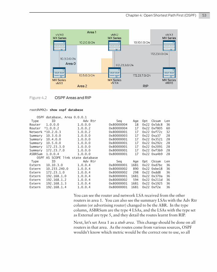
Chapter 4: Open Shortest Path First (OSPF) 53
Figure 4.2 OSPF Areas and RIP
root@VMX2> show ospf database
OSPF database, Area 0.0.0.1 Type ID Adv Rtr Seq Age Opt Cksum LenRouter 1.0.0.0 1.0.0.0 0x80000004 18 0x22 0x5dc8 36Router *1.0.0.2 1.0.0.2 0x80000004 17 0x22 0xf805 60Network *10.2.0.3 1.0.0.2 0x80000001 17 0x22 0xf72c 32Summary 10.3.0.0 1.0.0.0 0x80000003 17 0x22 0xa37 28Summary 10.4.0.0 1.0.0.0 0x80000001 17 0x22 0x3521 28Summary 10.5.0.0 1.0.0.0 0x80000001 17 0x22 0x292c 28Summary 172.23.3.0 1.0.0.0 0x80000001 17 0x22 0x2091 28Summary 172.23.7.0 1.0.0.0 0x80000001 17 0x22 0xf3b9 28ASBRSum 1.0.0.4 1.0.0.0 0x80000001 17 0x22 0xa4b9 28 OSPF AS SCOPE link state database Type ID Adv Rtr Seq Age Opt Cksum LenExtern 10.10.3.0 1.0.0.4 0x80000001 1681 0x22 0xd7bc 36Extern 10.233.240.0 1.0.0.4 0x80000002 890 0x22 0xbe18 36Extern 172.23.1.0 1.0.0.4 0x80000002 298 0x22 0xdd8 36Extern 192.168.1.0 1.0.0.4 0x80000001 1681 0x22 0x370a 36Extern 192.168.1.2 1.0.0.4 0x80000002 594 0x22 0x211d 36Extern 192.168.1.3 1.0.0.4 0x80000001 1681 0x22 0x1925 36Extern 192.168.1.4 1.0.0.4 0x80000001 1681 0x22 0xf2e 36
You can see the router and network LSA received from the other routers in area 1. You can also see the summary LSAs with the Adv Rtr column (or advertising router) changed to be the ABR. In the type column, ASBRSum are the type 4 LSAs, and the LSAs with the type set as External are type 5, and they detail the routes learnt from RIP.
Next, let’s set Area 1 as a stub area. This change should be done on all routers in that area. As the routes come from various sources, OSPF wouldn’t know which metric would be the correct one to use, so all

54 Day One: Routing the Internet Protocol
metrics are removed. To correct this, the default-metric option is used to inform OSPF which metric to apply to these routes. Without the default-metric keyword, the routes will not appear in the routing table:
[edit]root@VMX0# set protocols ospf area 1 stub default-metric 100
[edit]root@VMX2# set protocols ospf area 1 stub
NOTE The default-metric option need only be added to the ABR. Other routers in the area just need to be told they are in a stub area.
Now, if you look at the database, the change is very subtle, but the type 4 LSA has disappeared from the list:
root@VMX2> show ospf database
OSPF database, Area 0.0.0.1 Type ID Adv Rtr Seq Age Opt Cksum LenRouter 1.0.0.0 1.0.0.0 0x80000004 133 0x20 0x7bac 36Router *1.0.0.2 1.0.0.2 0x80000003 132 0x20 0x19e7 60Network *10.2.0.3 1.0.0.2 0x80000001 132 0x20 0x1610 32Summary 10.3.0.0 1.0.0.0 0x80000001 176 0x20 0x2c19 28Summary 10.4.0.0 1.0.0.0 0x80000001 176 0x20 0x5305 28Summary 10.5.0.0 1.0.0.0 0x80000001 176 0x20 0x4710 28Summary 172.23.3.0 1.0.0.0 0x80000001 176 0x20 0x3e75 28Summary 172.23.7.0 1.0.0.0 0x80000001 176 0x20 0x129d 28 OSPF AS SCOPE link state database Type ID Adv Rtr Seq Age Opt Cksum LenExtern 10.10.3.0 1.0.0.4 0x80000001 2205 0x22 0xd7bc 36Extern 10.233.240.0 1.0.0.4 0x80000002 1414 0x22 0xbe18 36Extern 172.23.1.0 1.0.0.4 0x80000002 822 0x22 0xdd8 36Extern 192.168.1.0 1.0.0.4 0x80000002 231 0x22 0x350b 36Extern 192.168.1.2 1.0.0.4 0x80000002 1118 0x22 0x211d 36Extern 192.168.1.3 1.0.0.4 0x80000001 2205 0x22 0x1925 36Extern 192.168.1.4 1.0.0.4 0x80000002 527 0x22 0xd2f 36
If you were to look at the routing table, you would see that the routes from RIP are now showing as a single default route to 0.0.0.0/0:
root@VMX2# run show route protocol ospf
inet.0: 19 destinations, 22 routes (19 active, 0 holddown, 0 hidden)+ = Active Route, - = Last Active, * = Both
0.0.0.0/0 *[OSPF/10] 00:00:12, metric 1100 > to 10.2.0.1 via ge-0/0/0.010.3.0.0/24 *[OSPF/10] 00:21:54, metric 2000 > to 10.2.0.1 via ge-0/0/0.010.4.0.0/24 *[OSPF/10] 00:21:54, metric 3000 > to 10.2.0.1 via ge-0/0/0.010.5.0.0/24 *[OSPF/10] 00:21:54, metric 3000 > to 10.2.0.1 via ge-0/0/0.0172.23.3.0/24 *[OSPF/10] 00:21:12, metric 4000 > to 10.2.0.1 via ge-0/0/0.0172.23.7.0/24 *[OSPF/10] 00:21:12, metric 4000

Chapter 4: Open Shortest Path First (OSPF) 55
> to 10.2.0.1 via ge-0/0/0.0224.0.0.5/32 *[OSPF/10] 00:22:51, metric 1 MultiRecv
Note that Area 1 can also be changed into a totally stubby area by adding the keyword no-summaries just before the default-metric option at the end of the previous command. This change need only be applied to ABRs, which in this case is vMX0:
[edit]root@VMX0# set protocols ospf area 1 stub no-summaries default-metric 100
After committing this change, the OSPF database appears very differ-ent with all summary LSAs removed:
root@VMX2> run show ospf database
OSPF database, Area 0.0.0.1 Type ID Adv Rtr Seq Age Opt Cksum LenRouter 1.0.0.0 1.0.0.0 0x80000007 47 0x20 0x61c5 36Router *1.0.0.2 1.0.0.2 0x80000008 7 0x20 0xfa03 60Network 10.2.0.1 1.0.0.0 0x80000001 47 0x20 0x3eeb 32 OSPF AS SCOPE link state database Type ID Adv Rtr Seq Age Opt Cksum LenExtern 10.10.3.0 1.0.0.4 0x80000001 2576 0x22 0xd7bc 36Extern 10.233.240.0 1.0.0.4 0x80000002 1785 0x22 0xbe18 36Extern 172.23.1.0 1.0.0.4 0x80000002 1193 0x22 0xdd8 36Extern 192.168.1.0 1.0.0.4 0x80000002 602 0x22 0x350b 36Extern 192.168.1.2 1.0.0.4 0x80000002 1489 0x22 0x211d 36Extern 192.168.1.3 1.0.0.4 0x80000001 2576 0x22 0x1925 36Extern 192.168.1.4 1.0.0.4 0x80000002 898 0x22 0xd2f 36
The routing table on vMX2 also looks very different with OSPF showing a single default route:
root@VMX2> show route protocol ospf
inet.0: 13 destinations, 15 routes (13 active, 0 holddown, 0 hidden)+ = Active Route, - = Last Active, * = Both
0.0.0.0/0 *[OSPF/10] 00:05:58, metric 1100 > to 10.2.0.1 via ge-0/0/0.0224.0.0.5/32 *[OSPF/10] 11:08:23, metric 1 MultiRecv
As you witnessed with stub areas, the ABR replaces the LSA type 4 with a default route. NSSA, or not so stubby areas, were created to allow redistribution of another routing protocol into OSPF via a stub area. This is done by replacing type 5 LSAs with a type 7 LSA.
In this next scenario, Area 2 will be made into an NSSA. Area 1 will be changed back to a stub area. As with stub areas, the default-metric option needs to be included. With NSSAs, the default-lsa option must also be included to tell the router to generate a default route.

56 Day One: Routing the Internet Protocol
Without it, the router will not add the default route to the routing table:
[edit]root@VMX1# set protocols ospf area 2 nssa default-lsa default-metric 100
[edit]root@VMX4# set protocols ospf area 2 nssa
Once committed, a default route is injected into area 2 which can be seen by looking at the routing table on router vMX4:
root@VMX4> show route protocol ospf
inet.0: 24 destinations, 29 routes (24 active, 0 holddown, 0 hidden)+ = Active Route, - = Last Active, * = Both
0.0.0.0/0 *[OSPF/150] 00:00:16, metric 1100, tag 0 > to 10.5.0.1 via ge-0/0/1.010.2.0.0/24 *[OSPF/10] 00:00:16, metric 3000 > to 10.5.0.1 via ge-0/0/1.010.3.0.0/24 *[OSPF/10] 00:00:16, metric 2000 > to 10.5.0.1 via ge-0/0/1.010.4.0.0/24 *[OSPF/10] 00:00:16, metric 2000 > to 10.5.0.1 via ge-0/0/1.010.10.1.0/24 *[OSPF/10] 00:00:16, metric 4000 > to 10.5.0.1 via ge-0/0/1.010.10.2.0/24 *[OSPF/10] 00:00:16, metric 4000 > to 10.5.0.1 via ge-0/0/1.0224.0.0.5/32 *[OSPF/10] 01:17:58, metric 1 MultiRecv
If Area 2 is made into a not so stubby totally stubby area by adding the no-summaries option, the results are similar to totally stubby areas in that all OSPF routes external to the area are summarized into a single default route:
[edit]root@VMX1# set protocols ospf area 0.0.0.2 nssa no-summaries default-lsa default-metric 100
root@VMX4> show route protocol ospf
inet.0: 21 destinations, 24 routes (21 active, 0 holddown, 0 hidden)+ = Active Route, - = Last Active, * = Both
0.0.0.0/0 *[OSPF/10] 00:00:07, metric 1100 > to 10.5.0.1 via ge-0/0/1.0224.0.0.5/32 *[OSPF/10] 01:16:06, metric 1 MultiRecv
Just as important, however, is that Area 1 is still receiving details of routes learned via RIP – meaning the LSAs are being allowed out of Area 2:
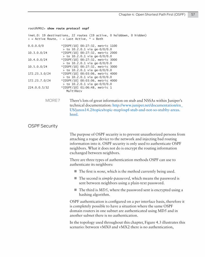
Chapter 4: Open Shortest Path First (OSPF) 57
root@VMX2> show route protocol ospf
inet.0: 19 destinations, 22 routes (19 active, 0 holddown, 0 hidden)+ = Active Route, - = Last Active, * = Both
0.0.0.0/0 *[OSPF/10] 00:27:32, metric 1100 > to 10.2.0.1 via ge-0/0/0.010.3.0.0/24 *[OSPF/10] 00:27:32, metric 2000 > to 10.2.0.1 via ge-0/0/0.010.4.0.0/24 *[OSPF/10] 00:27:32, metric 3000 > to 10.2.0.1 via ge-0/0/0.010.5.0.0/24 *[OSPF/10] 00:27:32, metric 3000 > to 10.2.0.1 via ge-0/0/0.0172.23.3.0/24 *[OSPF/10] 00:03:06, metric 4000 > to 10.2.0.1 via ge-0/0/0.0172.23.7.0/24 *[OSPF/10] 00:03:06, metric 4000 > to 10.2.0.1 via ge-0/0/0.0224.0.0.5/32 *[OSPF/10] 01:06:48, metric 1 MultiRecv
MORE? There’s lots of great information on stub and NSSAs within Juniper’s technical documentation: http://www.juniper.net/documentation/en_US/junos14.2/topics/topic-map/ospf-stub-and-not-so-stubby-areas.html.
OSPF Security
The purpose of OSPF security is to prevent unauthorized persons from attaching a rogue device to the network and injecting bad routing information into it. OSPF security is only used to authenticate OSPF neighbors. What it does not do is encrypt the routing information exchanged between neighbors.
There are three types of authentication methods OSPF can use to authenticate its neighbors:
� The first is none, which is the method currently being used.
� The second is simple-password, which means the password is sent between neighbors using a plain-text password.
� The third is MD5, where the password sent is encrypted using a hashing algorithm.
OSPF authentication is configured on a per interface basis, therefore it is completely possible to have a situation where the same OSPF domain routers in one subnet are authenticated using MD5 and in another subnet there is no authentication.
In the topology used throughout this chapter, Figure 4.3 illustrates this scenario: between vMX0 and vMX2 there is no authentication,

58 Day One: Routing the Internet Protocol
between vMX0 and vMX1 OSPF MD5 authentication is being used, and finally, the interfaces connecting vMX1 and vMX4 are using a simple password to authenticate.
Figure 4.3 OSPF Authentication Types
Although using simple-passwords is allowed in the Junos OS, this option was only included to comply with the OSPF standard and for backwards compatibility with older devices where performance could be affected by hashing passwords. As such, it is not recommended to use on a live network environment. It’s been included here in the configuration examples so you can see how this differs from configur-ing MD5 authentication.
Configuring OSPF Security
To keep this section simple, these OSPF authentication examples will be configured per Figure 4.3. No changes need to be applied to the link connecting vMX0 and vMX2. The interfaces connecting vMX1 and vMX4, however, do need to be enabled for simple password authenti-cation. This is done with the following configuration:
[edit]root@VMX1# set protocols ospf area 2 interface ge-0/0/2.0 authentication simple-password secretpd

Chapter 4: Open Shortest Path First (OSPF) 59
[edit]root@VMX4# set protocols ospf area 2 interface ge-0/0/1.0 authentication simple-password secretpd
There is one limitation to using simple password authentication and that is that the password must be eight characters or less. If the above configuration was attempted with the password secretpassword, the following error would appear during the commit:
[edit]root@VMX1# commit[edit protocols ospf area 0.0.0.2 interface ge-0/0/2.0] ‘authentication’ ospf password is longer than 8 characterserror: configuration check-out failed
If you use the now familiar show ospf neighbor command, you should see that the routers are still neighbors, meaning they have passed the authentication checks.
Next, routers vMX0 and vMX1 need to be configured for MD5 authentication, which enables a few more options for the administra-tor. The configuration begins as it does for the simple password, aside from changing the option from simple-password to md5, after which the administrator needs to specify a key between 0 and 255.
This key number allows the administrator to assign multiple pass-words to the interface (useful if an administrator wishes to change the passwords on the interfaces). Instead of deleting the old password and creating a new one, thereby risking losing connectivity, the administra-tor can just create a new key number and new password. The adminis-trator can also specify the date and time when the new key should be used, as you can see here with the possible completions:
[edit]root@VMX0# set protocols ospf area 0 interface ge-0/0/1.0 authentication md5 0 ?Possible completions: key MD5 authentication key value start-time Start time for key transmission (YYYY-MM-DD.HH:MM)
After this new key comes into effect, the old passwords can be deleted. In this scenario, routers vMX0 and vMX1 will use key 0 with no start time. The password of secretpassword will be used to illustrate that a longer password can be used:
set protocols ospf area 0.0.0.0 interface ge/0/1.0 authentication md5 0 key secretpassword
The best method to confirm these routers are authenticating correctly is to use the show ospf neighbor command. If the neighbors were showing as 2way, then it would be obvious there is a problem with authentication. In addition, you can use the show ospf overview command, and this command is covered in the next section.

60 Day One: Routing the Internet Protocol
OSPF Router IDs
Each router in the OSPF domain needs a unique router ID associated with it so it is identifiable to its neighbors, but also so when it appears in the database all other routers on the network know which subnets are associated with that ID.
As mentioned earlier, this ID is generated from the lowest IP address of all interfaces that are up. The issue with this is that when an interface goes down the ID can change, and as such the database needs updating and all routers in that area need to run the SPF algorithm once more. As an example, the output generated by the show interfaces terse command on a router with three interfaces that are up is:
show interfaces terseInterface Admin Link Proto Local Remotege-0/0/0.0 up up inet 10.0.1.1/24ge-0/0/1.0 up up inet 192.168.0.1/24ge-0/0/2.0 up up inet 172.23.7.1/24
From the three interfaces, interface ge-0/0/0.0 has the lowest IP address with 10.0.1.1. Should this interface go down, then the interface with the second lowest IP address, which is ge-0/0/2.0, will be used for the router ID, in which case the ID would become 172.23.7.1.
There are alternatives. One is to use a loopback interface because the loopback interface address will have a higher priority than the physical interface addresses. If an engineer creates an additional loopback interface when performing testing, then the same issue can arise.
Another option would be to specify the ID manually, which overrides the IDs from both the physical and loopback interfaces. No matter where the ID is sourced, the current ID of the router can be found by running the show ospf overview command:
root@VMX0> show ospf overviewInstance: master Router ID: 10.1.0.1 Route table index: 0 LSA refresh time: 50 minutes Area: 0.0.0.0 Stub type: Not Stub Authentication Type: None Area border routers: 0, AS boundary routers: 2 Neighbors Up (in full state): 2 Topology: default (ID 0) Prefix export count: 0 Full SPF runs: 20 SPF delay: 0.200000 sec, SPF holddown: 5 sec, SPF rapid runs: 3 Backup SPF: Not Needed
This command can be very useful when performing diagnostics as it also shows the areas attached to the router, the area type, the authenti-cation type if used, how many neighbors the router has, and the LSA

Chapter 4: Open Shortest Path First (OSPF) 61
refresh time, which is how often the router will refresh the database with new LSAs to ensure the LSA database matches those on other routers in that area.
The ID is set with the following command and the commit takes effect after the dead timer has reached 0:
set routing-options router-id 1.0.0.0
If the ID is set manually, it cannot use an address that begins with a zero. If this is attempted, then the following error will be displayed during a commit:
[edit]root@VMX0# commit[edit routing-options router-id] ‘router-id 0.0.0.1’ address invalid for routeriderror: configuration check-out failed [edit]root@VMX0# run show ospf overview | match Router | match ID Router ID: 1.0.0.0
Once a valid ID has been entered, running the show ospf overview command lists the new address:
[edit]root@VMX0# run show ospf overview | match Router | match ID Router ID: 1.0.0.0
It is also recommended to confirm that the neighbors see the change in the ID with the show ospf neighbors command:
[edit] root@VMX1# run show ospf neighborAddress Interface State ID Pri Dead10.4.0.2 ge-0/0/0.0 Full 10.4.0.2 128 3310.3.0.1 ge-0/0/1.0 Full 1.0.0.0 128 3710.5.0.2 ge-0/0/2.0 Full 10.5.0.2 128 31
OSPF Timers
To help make OSPF converge faster, OSPF utilizes timers similar to the way RIP does.
The Hello timer determines how often routers send a hello packet out of the interface to other routers. The time period needs to match on all routers on the subnet, otherwise they will appear to be stuck in ExStart in the neighbor table. The default timer on Ethernet networks and serial links is set to 10 seconds, or 30 seconds for frame relay.
Frame relay networks also have a timer called the Poll interval, because frame relay networks are typically non-broadcast, meaning the traditional method of finding neighbors by using multicast will not work. With frame relay networks, the administrator needs to add the neighbor manually. The poll interval determines how often the router

62 Day One: Routing the Internet Protocol
should send a message to the neighbor in order to form an adjacency. By default, this is set to 120 seconds.
When a router sends LSAs to its neighbors, it expects to receive a reply from its neighbor stating it received the LSA. If the router does not receive a reply within a certain amount of time, the router will resend the LSA. This is known as the LSA retransmission interval and by default this is set to five seconds.
The Dead interval is a period of time where the router has not received a hello packet from a neighbor and as such determines that the neigh-bor is down. For example, if vMX1 did not receive a hello packet from vMX0 for 40 seconds by default, then vMX1 would remove vMX0 from its neighbor table. The dead timer is typically four times the hello timer and on frame relay networks the dead timer is by default 120 seconds.
Finally, the purpose of the Transit delay is to increase the age of a link state update packet as it’s sent out of an interface. This is set by default to one second and ideally should never be changed.
Configuring OSPF Timers
Similar to authentication, timers are changed on a per interface basis. The following commands set the dead timer on vMX1’s interface connected to vMX0 to 4 seconds, the hello interval to 1 second and the LSA retransmission interval to 2 seconds:
[edit]root@VMX1# set protocols ospf area 0.0.0.0 interface ge-0/0/1.0 retransmit-interval 2
[edit]root@VMX1# set protocols ospf area 0.0.0.0 interface ge-0/0/1.0 hello-interval 1
[edit]root@VMX1# set protocols ospf area 0.0.0.0 interface ge-0/0/1.0 dead-interval 4
Unfortunately, after committing this configuration, vMX0 was removed from the neighbor table of vMX1 because it did not respond within the dead timer of 4 seconds (the hello timer on vMX0 is still set to 10 seconds):
root@VMX1> show ospf neighborAddress Interface State ID Pri Dead10.5.0.2 ge-0/0/2.0 Full 1.0.0.4 128 36
After setting the timers of vMX0 to match vMX1, the neighborship is restored:
[edit]root@VMX0# set protocols ospf area 0.0.0.0 interface ge-0/0/1.0 retransmit-interval 2

Chapter 4: Open Shortest Path First (OSPF) 63
[edit]root@VMX0# set protocols ospf area 0.0.0.0 interface ge-0/0/1.0 hello-interval 1
[edit]root@VMX0# set protocols ospf area 0.0.0.0 interface ge-0/0/1.0 dead-interval 4
And let’s verify neighbors:
root@VMX1> show ospf neighborAddress Interface State ID Pri Dead10.3.0.1 ge-0/0/1.0 Full 1.0.0.0 128 310.5.0.2 ge-0/0/2.0 Full 1.0.0.4 128 34
Notice how under the dead column the number is now 3 compared to 34 for the connection to vMX4. Should router vMX0 suddenly fail for what-ever reason, vMX1 would remove it from the neighbor table very quickly.
Discontiguous OSPF Areas
Occasionally a situation may arise where you have no choice but to connect a non-backbone OSPF area to an area other than Area 0, such as in the case of an acquisition or merger. In this case it becomes necessary to break the OSPF Area 0 rule. To do this an engineer can use what is known as a virtual link. Figure 4.4 shows an example of what is known as a discontiguous area where Area 80 needs to cross Area 1 to reach Area 0.
Figure 4.4 OSPF Virtual Links

64 Day One: Routing the Internet Protocol
With a virtual link a tunnel is created across the area that is between Area 0 and the new area that is cut off from Area 0, in Figure 4.4 the tunnel would cross Area 1. The configuration to allow this is placed on the ABRs of the area that is to be crossed. The routers inside Area 80 wouldn’t know they were crossing a tunnel; as far as they are aware, they are directly connected to Area 0.
If the routers are configured as in Figure 4.4, but without the virtual link, and you look at the routing table on router vMX2, you would observe that vMX0’s interface in subnet 10.3.0.0/24 appears in the routing table, but no other routes are discovered:
root@VMX2> show route protocol ospf
inet.0: 13 destinations, 15 routes (13 active, 0 holddown, 0 hidden)+ = Active Route, - = Last Active, * = Both
10.3.0.0/24 *[OSPF/10] 00:03:52, metric 2 > to 10.2.0.1 via ge-0/0/0.0224.0.0.5/32 *[OSPF/10] 05:22:11, metric 1 MultiRecv
To resolve this issue, the set protocols ospf area 0 virtual-link command is used in the routers vMX0 and vMX1. After neighbor-id the administrator is required to add the router ID of the ABR at the other end of the tunnel, for example, for router vMX0, you would specify the ID of vMX1 and for vMX1 you would enter the ID for vMX0. The final part of the command tells the router which area the tunnel transits:
[edit]root@VMX0# set protocols ospf area 0 virtual-link neighbor-id 1.0.0.1 transit-area 0.0.0.1
[edit]root@VMX1# set protocols ospf area 0 virtual-link neighbor-id 1.0.0.0 transit-area 0.0.0.1
Now, let’s look at the routing table on vMX2, and you should see all routes discovered as advertised via OSPF:
root@VMX2> show route protocol ospf
inet.0: 23 destinations, 26 routes (23 active, 0 holddown, 0 hidden)+ = Active Route, - = Last Active, * = Both
10.3.0.0/24 *[OSPF/10] 00:15:43, metric 2 > to 10.2.0.1 via ge-0/0/0.010.4.0.0/24 *[OSPF/10] 00:01:11, metric 3 > to 10.2.0.1 via ge-0/0/0.010.5.0.0/24 *[OSPF/10] 00:01:11, metric 3 > to 10.2.0.1 via ge-0/0/0.0172.23.3.0/24 *[OSPF/10] 00:01:11, metric 4 > to 10.2.0.1 via ge-0/0/0.0172.23.7.0/24 *[OSPF/10] 00:01:11, metric 4 > to 10.2.0.1 via ge-0/0/0.0224.0.0.5/32 *[OSPF/10] 05:34:02, metric 1 MultiRecv

Chapter 4: Open Shortest Path First (OSPF) 65
Finally, if the show ospf neighbors command were to be run, an additional neighbor will appear in the list with the same ID as the ABR in area 0 but instead showing the outgoing interface as vl-1.0.0.1. This interface is the virtual link between routers vMX0 and vMX1:
root@VMX0> show ospf neighborAddress Interface State ID Pri Dead10.3.0.2 ge-0/0/1.0 Full 1.0.0.1 128 3710.2.0.3 ge-0/0/2.0 Full 1.0.0.2 128 3610.3.0.2 vl-1.0.0.1 Full 1.0.0.1 0 35
OSPF Overload Function
The last OSPF feature before moving onto IS-IS is something called the OSPF overload function. This feature is something you probably wouldn’t run too often, but it can be quite useful. It makes the router appear that it is overloaded to other routers on the network, and as such can no longer participate in normal routing on the network.
There are two situations in which an administrator may want to use this function. The first is when the administrator would like the router to receive routes, but not to participate in routing itself, for example, when a router is being used for analysis of network traffic.
The second situation is when the administrator is performing mainte-nance and doesn’t want the router to be used as a transit router, but wants the router to remain up so it can be brought into service much sooner.
The command that enables overload is added to the whole OSPF routing process. It is not possible to set this command for a particular area only. The command also allows the administrator to specify a time out period. If no timeout option is set, then the overload is set until the configuration is removed. The timeout period can be set from 60 seconds to 1800 seconds. The default is 0.
Once the command is added, the router still advertises routes it has learned, except that the metric will be set to 65535 or infinite, meaning the neighbors will still receive the routes, but will mark them as inaccessible, and as a result they will not be entered into their local routing tables.
The command to enable overload is as follows. In this case, the timeout is set to 180 seconds, which means in 3 minutes the router will return to normal operation:
set protocols ospf overload timeout 180
OSPF overload function: If the time elapsed after the OSPF instance is enabled is less than the specified timeout, overload mode is set .
http://www .juniper .net/documentation/en_US/junos12 .3/topics/concept/ospf-overload-function-overview .html

66 Day One: Routing the Internet Protocol
Summary
OSPF is a popular protocol amongst network engineers. The scalabil-ity of this protocol means a network administrator may never need to migrate to another protocol. The only downside is that it is more complex to implement compared to RIP or static routes.
The key to OSPF’s scalability lies with its use of areas. Understanding the use of areas will become useful during the next chapter when you look at a protocol that can scale to a size beyond the capabilities of OSPF.
This chapter shared some useful information about the Junos OS and OSPF, however, if you are interested, further information can be found at the Juniper TechLibrary and readers might start at this OSPF pathway page: https://www.juniper.net/techpubs/en_US/junos14.1/information-products/pathway-pages/config-guide-routing/config-guide-ospf.html.
Also, follow these examples in your own lab if you can. It greatly aids in the learning process.

Like OSPF, IS-IS is also a link state routing protocol. It uses the same SPF algorithm and is scalable, even more so than OSPF. However, IS-IS has a very different history than OSPF and that is because it was never designed to advertise IP subnets, and was in fact designed for another routed protocol, called OSI.
Back in the early 1990s, a company called Digital Equipment Corpora-tion (DEC), developed and standardized the OSI protocol. At the same time, the IETF developed another protocol called the Internet Protocol, or IP. These protocols were in direct competition with each other, and not knowing which to support service providers had both protocols running on their networks.
IP obviously became the dominant protocol, although it was discov-ered that OSI did have a useful feature in that the packets it sends across the network, known as Protocol Data Units (PDUs) are com-prised of Type Length Value (TLVs). These TLVs can be used to exchange routing information, usually IP, but OSI was very easily adapted to advertise IPv6 routing information.
So, the one major difference between IS-IS and other routing protocols is that IS-IS does not use IP as the transport protocol, and instead uses OSI. So any router that uses IS-IS to advertise routes must have OSI enabled, and an address configured, which is another major difference compared to IP. With IP, each interface is given an address in a different subnet, while with OSI the router as a whole is given a single address, usually to the loopback interface.
The address in OSI is made up of several components, rather like an IP address is divided into the network address and host address, but unlike IP, the OSI address is made up of four parts:
Chapter 5
Intermediate System to Intermediate System (IS-IS)
Internet Protocol: The principal communications protocol in the Internet protocol suite for relaying datagrams across network boundaries:
https://en .wikipedia .org/wiki/Internet_Protocol

68 Day One: Routing the Internet Protocol
1. AFI: Authority and Format Indicator. This identifies the type of device this address is assigned to. For routers, this will always be set as 49.
2. Area ID: This part is similar to IPv4 subnet addresses. Routers in the same level will use the same area ID. Levels will be explained in the following Configuring IS-IS section.
3. System ID: Similar to an IPv4 host address. Each router must have a unique number. This cannot be all 0s but can be hexadecimal.
4. N-selector: Always set as 00.
Figure 5.1 shows an example of an OSI address where the address has been assigned to a router in Area 1 with an address of 0001.0001.00001.
Figure 5.1 OSI Address
Configuring IS-IS
Figure 5.2 shows the topology of the network that will be used in this configuration example.
Figure 5.2 IS-IS Topology

Chapter 5: Intermediate System to Intermediate System (IS-IS) 69
As shown in Figure 5.2, IS-IS neighborships are formed between routers vMX3, vMX2, vMX5, and vMX6, however the subnet between routers vMX3 and vMX6 is part of the RIP domain that will later be redistrib-uted into IS-IS, therefore these interfaces will not send hello PDUs.
The first step is to assign an OSI address to each router. Each router is in area 0001 and the address assigned to the interface is loopback 0.0 and the /32 IP address will be assigned to this interface. In addition, OSI needs to be enabled on each interface that sends PDUs. The first router to be configured is vMX2:
set interfaces lo0 unit 0 family inet address 192.168.1.1/32set interfaces lo0 unit 0 family iso address 49.0001.0001.0001.0001.00set interfaces ge-0/0/0 unit 0 family isoset interfaces ge-0/0/1 unit 0 family isoset interfaces ge-0/0/2 unit 0 family iso
Next, router vMX3 is given a different /32 address and a different OSI address:
set interfaces lo0 unit 0 family inet address 192.168.1.2/32set interfaces lo0 unit 0 family iso address 49.0001.0001.0001.0002.00set interfaces ge-0/0/0 unit 0 family isoset interfaces ge-0/0/1 unit 0 family isoset interfaces ge-0/0/2 unit 0 family iso
Now vMX5 is configured as follows:
set interfaces lo0 unit 0 family inet address 192.168.1.3/24set interfaces lo0 unit 0 family iso address 49.0001.0001.0001.0003.00set interfaces ge-0/0/0 unit 0 family isoset interfaces ge-0/0/1 unit 0 family iso
And vMX6 is given the OSI System ID of 0001.0001.0004:
set interfaces lo0 unit 0 family inet address 192.168.1.4/24set interfaces lo0 unit 0 family iso address 49.0001.0001.0001.0004.00set interfaces ge-0/0/0 unit 0 family isoset interfaces ge-0/0/1 unit 0 family isoset interfaces ge-0/0/2 unit 0 family iso
Now, all routers have been given an address and OSI is enabled on all interfaces, so let’s tell IS-IS which interfaces to advertise and which not to send hello PDUs out of. Similar to RIP and OSPF, the passive option tells IS-IS not to send hello PDUs out of that interface. Router vMX2’s interface ge-0/0/0.0 is part of the OSPF domain, therefore set this as passive:
set protocols isis interface ge-0/0/0.0 passiveset protocols isis interface ge-0/0/1.0 set protocols isis interface ge-0/0/2.0set protocols isis interface lo0.0
Interfaces ge-0/0/0.0 and ge-0/0/2.0 on router vMX3 are part of the RIP domain, therefore these too are set as passive:
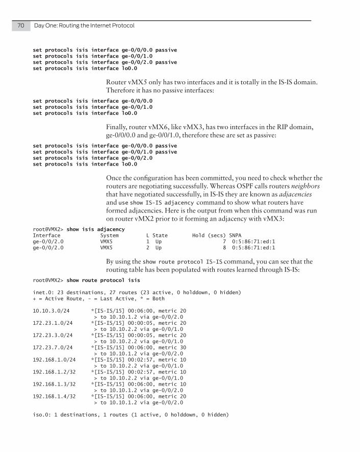
70 Day One: Routing the Internet Protocol
set protocols isis interface ge-0/0/0.0 passiveset protocols isis interface ge-0/0/1.0set protocols isis interface ge-0/0/2.0 passiveset protocols isis interface lo0.0
Router vMX5 only has two interfaces and it is totally in the IS-IS domain. Therefore it has no passive interfaces:
set protocols isis interface ge-0/0/0.0set protocols isis interface ge-0/0/1.0set protocols isis interface lo0.0
Finally, router vMX6, like vMX3, has two interfaces in the RIP domain, ge-0/0/0.0 and ge-0/0/1.0, therefore these are set as passive:
set protocols isis interface ge-0/0/0.0 passiveset protocols isis interface ge-0/0/1.0 passiveset protocols isis interface ge-0/0/2.0set protocols isis interface lo0.0
Once the configuration has been committed, you need to check whether the routers are negotiating successfully. Whereas OSPF calls routers neighbors that have negotiated successfully, in IS-IS they are known as adjacencies and use show IS-IS adjacency command to show what routers have formed adjacencies. Here is the output from when this command was run on router vMX2 prior to it forming an adjacency with vMX3:
root@VMX2> show isis adjacencyInterface System L State Hold (secs) SNPAge-0/0/2.0 VMX5 1 Up 7 0:5:86:71:ed:1ge-0/0/2.0 VMX5 2 Up 8 0:5:86:71:ed:1
By using the show route protocol IS-IS command, you can see that the routing table has been populated with routes learned through IS-IS:
root@VMX2> show route protocol isis
inet.0: 23 destinations, 27 routes (23 active, 0 holddown, 0 hidden)+ = Active Route, - = Last Active, * = Both
10.10.3.0/24 *[IS-IS/15] 00:06:00, metric 20 > to 10.10.1.2 via ge-0/0/2.0172.23.1.0/24 *[IS-IS/15] 00:00:05, metric 20 > to 10.10.2.2 via ge-0/0/1.0172.23.3.0/24 *[IS-IS/15] 00:00:05, metric 20 > to 10.10.2.2 via ge-0/0/1.0172.23.7.0/24 *[IS-IS/15] 00:06:00, metric 30 > to 10.10.1.2 via ge-0/0/2.0192.168.1.0/24 *[IS-IS/15] 00:02:57, metric 10 > to 10.10.2.2 via ge-0/0/1.0192.168.1.2/32 *[IS-IS/15] 00:02:57, metric 10 > to 10.10.2.2 via ge-0/0/1.0192.168.1.3/32 *[IS-IS/15] 00:06:00, metric 10 > to 10.10.1.2 via ge-0/0/2.0192.168.1.4/32 *[IS-IS/15] 00:06:00, metric 20 > to 10.10.1.2 via ge-0/0/2.0
iso.0: 1 destinations, 1 routes (1 active, 0 holddown, 0 hidden)

Chapter 5: Intermediate System to Intermediate System (IS-IS) 71
Then best practice is to send a simple ping from router vMX3 to one of vMX6’s interfaces. A reply will prove connectivity is working as expected, and as shown below, all is fine:
root@VMX3> ping 172.23.7.2PING 172.23.7.2 (172.23.7.2): 56 data bytes64 bytes from 172.23.7.2: icmp_seq=0 ttl=63 time=14.644 ms64 bytes from 172.23.7.2: icmp_seq=1 ttl=63 time=4.951 ms64 bytes from 172.23.7.2: icmp_seq=2 ttl=63 time=4.533 ms^C--- 172.23.7.2 ping statistics ---3 packets transmitted, 3 packets received, 0% packet lossround-trip min/avg/max/stddev = 4.533/8.043/14.644/4.671 ms
IS-IS Areas
Like OSPF, IS-IS can scale to a considerable size, a size beyond that of OSPF and some say a size that can rival BGP. It achieves this scalability in the same way via the use of areas. IS-IS areas are slightly different from OSPF in that IS-IS uses levels to designate which areas are the backbone and which are not backbone.
With IS-IS, there are two levels. Any routers that are designated as level 1 are non-backbone area routers. Level 2 is the backbone area, similar to OSPF area 0.0.0.0. Level 2 areas should be contiguous.
Levels are assigned on a per-interface basis and any router that has one interface set as Level 2, and another set as Level 1, is an ABR, similar to OSPF. Figure 5.3 illustrates an example IS-IS domain with multiple routers in Level 2 and three ABRs with Level 1 routers attached, Areas X, Y, and Z, purely to illustrate that these are areas separate unto themselves.
Figure 5.3 An Example of IS-IS Levels

72 Day One: Routing the Internet Protocol
Configuring IS-IS Areas
Figure 5.4 shows how the routers will be configured. Router vMX3 is a Level 1 router in Area 2. Router vMX6 is a Level 1 router in Area 3, and routers vMX2 and vMX5 will be ABRs.
Figure 5.4 The Configuration Topology for IS-IS
By default, both Levels 1 and 2 are enabled on all interfaces that form an adjacency. Therefore, to set an interface as part of Level 2, instead of enabling Level 2, you need to disable Level 1. And likewise, to set an interface to be part of Level 1, you need to disable Level 2. Router vMX2 is an ABR and interface ge-0/0/1.0 will be a Level 1 interface and interface ge-0/0/2.0 will be a Level 2 interface. The commands to configure the router this way are:
set protocols isis interface ge-0/0/1.0 level 2 disableset protocols isis interface ge-0/0/2.0 level 1 disable
Router vMX3 only has one interface forming an adjacency and it is a Level 1 interface:
set protocols isis interface ge-0/0/1.0 level 2 disable
As router vMX5 is an ABR, one of its interfaces is set with Level 2 disabled and the other is set with level 1 disabled:
set protocols isis interface ge-0/0/0.0 level 2 disableset protocols isis interface ge-0/0/1.0 level 1 disable
Router vMX6 is similar to vMX3 in that it too only has one interface forming an adjacency so Level 2 is disabled:
set protocols isis interface ge-0/0/2.0 level 2 disable

Chapter 5: Intermediate System to Intermediate System (IS-IS) 73
Now that the configuration has been committed on all routers, the simplest but most reliable test is to send a ping and then look at the routing table. And as you can see, there is an issue. Router vMX6 can only see one route coming from router vMX5:
root@VMX6> show route protocol isis
inet.0: 13 destinations, 15 routes (13 active, 0 holddown, 0 hidden)+ = Active Route, - = Last Active, * = Both
192.168.1.3/32 *[IS-IS/15] 00:06:53, metric 10 > to 10.10.3.1 via ge-0/0/2.0
This issue was caused because the areas in the addresses were not changed. IS-IS sees that there are two Level 1 areas but they all have the same area in the address, which confuses IS-IS. To resolve this issue, the addresses need to be changed. The ABRs need their areas to be set to the Level 1 area they are adjoining. Router vMX2 is adjoining Area 2:
set interfaces lo0 unit 0 family iso address 49.0002.0001.0001.0001.00
Router vMX is wholly within Area 2:
set interfaces lo0 unit 0 family iso address 49.0002.0001.0001.0002.00
The second ABR is router vMX5. This is adjoining area 3:
set interfaces lo0 unit 0 family iso address 49.0003.0001.0001.0003.00
Finally, router vMX6 is completely in Area 3:
set interfaces lo0 unit 0 family iso address 49.0003.0001.0001.0004.00
Once the configuration has been committed, the routing table should now have one more route and that is a default route. Areas help make IS-IS scalable by summarizing all routes going into an area as a single default route. The routers inside the area only need to know that to reach a subnet that’s not listed in the routing table they just need to forward their packet to the ABR who has a complete routing table:
root@VMX6> show route protocol isis
inet.0: 14 destinations, 16 routes (14 active, 0 holddown, 0 hidden)+ = Active Route, - = Last Active, * = Both
0.0.0.0/0 *[IS-IS/15] 00:02:28, metric 10 > to 10.10.3.1 via ge-0/0/2.0192.168.1.3/32 *[IS-IS/15] 00:55:15, metric 10 > to 10.10.3.1 via ge-0/0/2.0
iso.0: 2 destinations, 2 routes (2 active, 0 holddown, 0 hidden)
Now, if router vMX6 pings router vMX3’s ge-0/0/0.0 interface, router vMX6 should receive a successful reply:
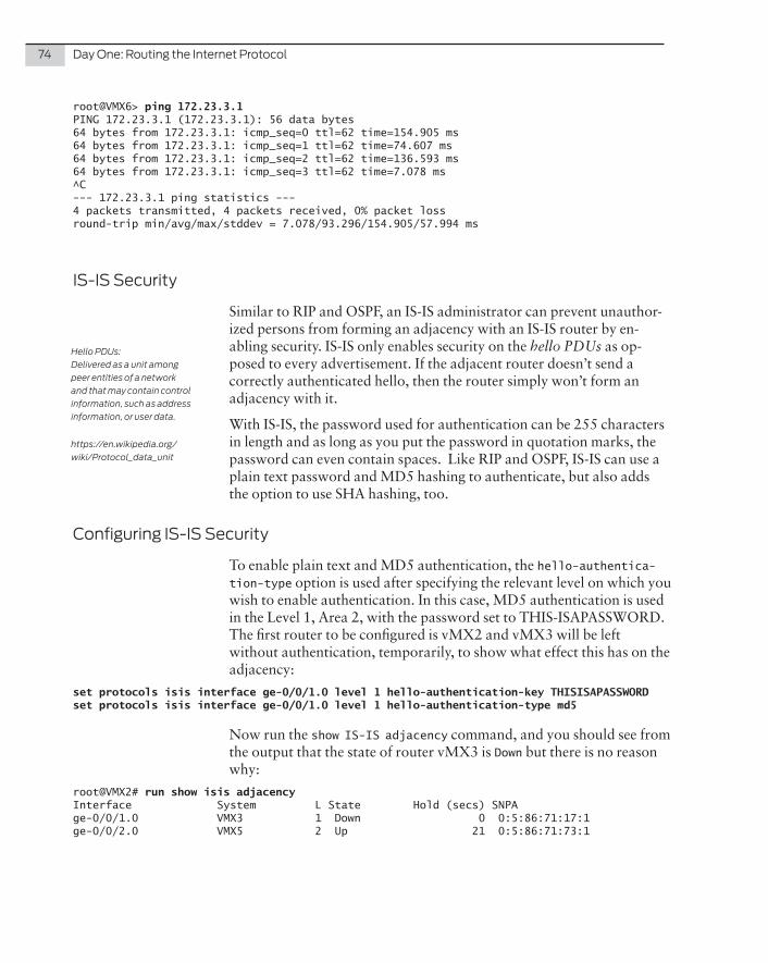
74 Day One: Routing the Internet Protocol
Hello PDUs: Delivered as a unit among peer entities of a network and that may contain control information, such as address information, or user data .
https://en .wikipedia .org/wiki/Protocol_data_unit
root@VMX6> ping 172.23.3.1PING 172.23.3.1 (172.23.3.1): 56 data bytes64 bytes from 172.23.3.1: icmp_seq=0 ttl=62 time=154.905 ms64 bytes from 172.23.3.1: icmp_seq=1 ttl=62 time=74.607 ms64 bytes from 172.23.3.1: icmp_seq=2 ttl=62 time=136.593 ms64 bytes from 172.23.3.1: icmp_seq=3 ttl=62 time=7.078 ms^C--- 172.23.3.1 ping statistics ---4 packets transmitted, 4 packets received, 0% packet lossround-trip min/avg/max/stddev = 7.078/93.296/154.905/57.994 ms
IS-IS Security
Similar to RIP and OSPF, an IS-IS administrator can prevent unauthor-ized persons from forming an adjacency with an IS-IS router by en-abling security. IS-IS only enables security on the hello PDUs as op-posed to every advertisement. If the adjacent router doesn’t send a correctly authenticated hello, then the router simply won’t form an adjacency with it.
With IS-IS, the password used for authentication can be 255 characters in length and as long as you put the password in quotation marks, the password can even contain spaces. Like RIP and OSPF, IS-IS can use a plain text password and MD5 hashing to authenticate, but also adds the option to use SHA hashing, too.
Configuring IS-IS Security
To enable plain text and MD5 authentication, the hello-authentica-tion-type option is used after specifying the relevant level on which you wish to enable authentication. In this case, MD5 authentication is used in the Level 1, Area 2, with the password set to THIS-ISAPASSWORD. The first router to be configured is vMX2 and vMX3 will be left without authentication, temporarily, to show what effect this has on the adjacency:
set protocols isis interface ge-0/0/1.0 level 1 hello-authentication-key THISISAPASSWORDset protocols isis interface ge-0/0/1.0 level 1 hello-authentication-type md5
Now run the show IS-IS adjacency command, and you should see from the output that the state of router vMX3 is Down but there is no reason why:
root@VMX2# run show isis adjacencyInterface System L State Hold (secs) SNPAge-0/0/1.0 VMX3 1 Down 0 0:5:86:71:17:1ge-0/0/2.0 VMX5 2 Up 21 0:5:86:71:73:1

Chapter 5: Intermediate System to Intermediate System (IS-IS) 75
If the extensive option is added to the end of the command, however, then you can clearly see that the reason for the down adjacency is because of a bad Hello. The hello is bad because it has no authentica-tion and that is not what vMX2 expects:
root@VMX2# run show isis adjacency VMX3 extensiveVMX3 Interface: ge-0/0/1.0, Level: 1, State: Down, Expires in 0 secs Priority: 64, Up/Down transitions: 2, Last transition: 00:00:35 ago Circuit type: 1, Speaks: IP, IPv6, MAC address: 0:5:86:71:17:1 Topologies: Unicast Restart capable: Yes, Adjacency advertisement: Advertise LAN id: VMX2.02, IP addresses: 10.10.2.2 Transition log: When State Event Down reason Thu Jun 11 11:43:40 Up Seenself Thu Jun 11 11:44:27 Down Error Bad Hello
So once the same commands are added to vMX3, the adjacency is restored:
set protocols isis interface ge-0/0/1.0 level 1 hello-authentication-key THISISAPASSWORDset protocols isis interface ge-0/0/1.0 level 1 hello-authentication-type md5
As mentioned earlier, IS-IS has an option for both MD5 and SHA authentication, the latter being a more secure method. SHA authenti-cation cannot be enabled by using the hello-authentication-type command and instead needs to be enabled with a key-chain.
Key chains have an advantage over just setting the adjacency’s type, in that the administrator can configure options such as setting different authentication keys and then setting the date when that key is valid, thereby allowing the administrator to migrate to new keys on a regular basis without causing any downtime.
It is still possible to use MD5 authentication from a key chain, how-ever it is not possible to use plain text. In this next scenario, two key chains will be configured: key 1 uses MD5 with the password set as “THIS-ISSECRET,” and key 2 uses SHA and the password is “THIS-ISSECRETTOO”. Key 1 is set to start at 16:00 on June 10th 2015 and key 2 begins on September 2nd 2015 at midnight:
set security authentication-key-chains key-chain ISIS-KEY-CHAIN key 1 secret THISISSECRETset security authentication-key-chains key-chain ISIS-KEY-CHAIN key 1 start-time 2015-06-10.16:00set security authentication-key-chains key-chain ISIS-KEY-CHAIN key 1 algorithm md5set security authentication-key-chains key-chain ISIS-KEY-CHAIN key 2 secret THISISSECRETTOOset security authentication-key-chains key-chain ISIS-KEY-CHAIN key 2 start-time 2015-9-2.00:00set security authentication-key-chains key-chain ISIS-KEY-CHAIN key 2 algorithm hmac-sha-1set security authentication-key-chains key-chain ISIS-KEY-CHAIN key 2 options isis-enhanced

76 Day One: Routing the Internet Protocol
NOTE If SHA authentication is to be used, the isis-enhanced option must be enabled, too. If it isn’t enabled, the Junos OS will not allow you to commit the configuration and will warn you.
All that remains to be done is to apply these keys to the relevant interfaces. In this scenario, authentication is enabled on the Level 2 backbone between routers vMX2 and vMX5, leaving the Level 1 authentication in place between vMX2 and vMX3 (just to prove that both authentication types can be used on the same router at the same time). Router vMX2’s Level 2 interface is ge-0/0/2.0:
set protocols isis interface ge-0/0/2.0 level 2 hello-authentication-key-chain ISIS-KEY-CHAIN
And router vMX5’s Level 2 interface is ge-0/0/1.0:
set protocols isis interface ge-0/0/1.0 level 2 hello-authentication-key-chain ISIS-KEY-CHAIN
After committing the configuration, the adjacency should be checked to prove the routers are authenticating each other correctly:
root@VMX5# run show isis adjacency briefInterface System L State Hold (secs) SNPAge-0/0/0.0 VMX6 1 Up 6 0:5:86:71:98:2ge-0/0/1.0 VMX2 2 Up 6 0:5:86:71:9a:2
IS-IS Reference Bandwidth
Like OSPF, IS-IS can use a reference bandwidth as the metric divided by the speed of the interface. Unlike OSPF, by default, IS-IS does not use a reference bandwidth and instead gives each interface a metric of 10. This means that all routes in the routing table will show a metric of 10, 20, 30 and so on depending on how many hops away the subnet is. By running the show route protocol IS-IS command, you can see the metrics:
root@VMX2> show route protocol isis
inet.0: 22 destinations, 27 routes (22 active, 0 holddown, 0 hidden)+ = Active Route, - = Last Active, * = Both
10.10.3.0/24 *[IS-IS/18] 00:06:00, metric 20 > to 10.10.1.2 via ge-0/0/2.0172.23.1.0/24 *[IS-IS/15] 00:00:05, metric 20 > to 10.10.2.2 via ge-0/0/1.0172.23.3.0/24 *[IS-IS/15] 00:00:05, metric 20 > to 10.10.2.2 via ge-0/0/1.0172.23.7.0/24 *[IS-IS/18] 00:06:00, metric 30 > to 10.10.1.2 via ge-0/0/2.0192.168.1.0/24 *[IS-IS/15] 00:02:57, metric 10 > to 10.10.2.2 via ge-0/0/1.0192.168.1.2/32 *[IS-IS/15] 00:02:57, metric 10 > to 10.10.2.2 via ge-0/0/1.0

Chapter 5: Intermediate System to Intermediate System (IS-IS) 77
192.168.1.3/32 *[IS-IS/18] 00:06:00, metric 10 > to 10.10.1.2 via ge-0/0/2.0192.168.1.4/32 *[IS-IS/18] 00:06:00, metric 20 > to 10.10.1.2 via ge-0/0/2.0
In reality, this default setting makes IS-IS’s behavior similar to that of RIP, using hops to determine the best route. Instead of using the default behavior, it is better to set a reference bandwidth.
The reference-bandwidth option needs to be set on all routers in the IS-IS domain and should ideally be set to a higher interface speed than is currently running on the network to allow for future proofing. In this instance, the reference bandwidth is set to 100Gb/s, like this:
set reference-bandwidth 100g
Once this setting has been added and committed to all routers, the metrics in the routing table should look bigger, for example, before the reference bandwidth was added the route to subnet 10.10.3.0/24 had a metric of 20. Once the reference bandwidth was added, the metric increased to 126:
root@VMX2> show route protocol isis
inet.0: 22 destinations, 27 routes (22 active, 0 holddown, 0 hidden)+ = Active Route, - = Last Active, * = Both
10.10.3.0/24 *[IS-IS/18] 00:00:35, metric 126 > to 10.10.1.2 via ge-0/0/2.0172.23.1.0/24 *[IS-IS/15] 00:00:29, metric 126 > to 10.10.2.2 via ge-0/0/1.0172.23.3.0/24 *[IS-IS/15] 00:00:29, metric 126 > to 10.10.2.2 via ge-0/0/1.0172.23.7.0/24 *[IS-IS/18] 00:00:34, metric 126 > to 10.10.1.2 via ge-0/0/2.0192.168.1.0/24 *[IS-IS/15] 00:00:35, metric 63 > to 10.10.2.2 via ge-0/0/1.0192.168.1.2/32 *[IS-IS/15] 00:00:35, metric 63 > to 10.10.2.2 via ge-0/0/1.0192.168.1.3/32 *[IS-IS/18] 00:00:35, metric 63 > to 10.10.1.2 via ge-0/0/2.0192.168.1.4/32 *[IS-IS/18] 00:00:34, metric 126 > to 10.10.1.2 via ge-0/0/2.0
IS-IS Timers
Like OSPF and RIP, IS-IS also allows an administrator to adjust the timers that help IS-IS decide when a router has lost an adjacency. There are two timers of note that can assist with this.
� To determine how often a hello PDU is sent out of the configured interfaces, an administrator can configure a hello-interval. This setting can be set from 1 to 20,000 seconds. The default setting is 3 seconds.

78 Day One: Routing the Internet Protocol
� The second timer is the hold-time option, which determines how long the router should wait after not receiving a hello before it declares the adjacent router down. This can be set from 3 to 65,535 seconds and has a default setting of 9.
Interestingly, if both the hold time and hello interval timers are set to 1, then the hello PDUs are sent every 333 milliseconds allowing for much faster route removal and an alternative route being found.
Configuring IS-IS Timers
Before changing the timers on your production networks, it’s a good idea to remember that this change is made at a time of day when any potential outage won’t affect anyone.
To check what the timers are currently set to, use the show IS-IS interface command along with the extensive option. In the follow-ing example, the command was run on router vMX2 and the output shows that the hello interval is set to 3.000 s and the hold time is 9 s. This command also shows that level 1 on this interface is disabled:
root@VMX2# run show isis interface ge-0/0/2.0 extensiveIS-IS interface database:ge-0/0/2.0 Index: 332, State: 0x6, Circuit id: 0x3, Circuit type: 2 LSP interval: 100 ms, CSNP interval: 10 s, Loose Hello padding Adjacency advertisement: Advertise Level 1 Adjacencies: 0, Priority: 64, Metric: 63 Disabled Level 2 Adjacencies: 1, Priority: 64, Metric: 63 Hello Interval: 3.000 s, Hold Time: 9 s Designated Router: VMX2.03 (us)
In this next scenario, the level 2 interfaces are set with a sub-second hello interval. The first router is vMX2:
set protocols isis interface ge-0/0/2.0 level 2 hello-interval 1set protocols isis interface ge-0/0/2.0 level 2 hold-time 1
Then the same commands are set on router vMX5:
set protocols isis interface ge-0/0/1.0 level 2 hello-interval 1set protocols isis interface ge-0/0/1.0 level 2 hold-time 1
By running the show IS-IS interface command again, you can see that the hello interval is now 0.333 s:
root@VMX2# run show isis interface ge-0/0/2.0 extensiveIS-IS interface database:ge-0/0/2.0 Index: 332, State: 0x6, Circuit id: 0x3, Circuit type: 2 LSP interval: 100 ms, CSNP interval: 10 s, Loose Hello padding

Chapter 5: Intermediate System to Intermediate System (IS-IS) 79
Adjacency advertisement: Advertise Level 1 Adjacencies: 0, Priority: 64, Metric: 63 Disabled Level 2 Adjacencies: 1, Priority: 64, Metric: 63 Hello Interval: 0.333 s, Hold Time: 1 s Designated Router: VMX2.03 (us)
Summary
Typically, IS-IS is used by service providers and not in corporate LANs. Its sheer scalability and faster convergence meet the demands of this type of network. There is of course no reason why IS-IS can’t be used by a company and for companies with many hundreds of subnets, IS-IS is a better choice. Some say IS-IS can scale to a size that rivals BGP whereas OSPF can never scale to that level.
After reading this chapter you should have a much better understand-ing of the alternative protocol to OSPF whilst reaffirming your under-standing of areas. This may also help you later in your career if you find yourself working for a service provider.
This brings us to the end of the last interior gateway protocol (IGP) covered in this book. The next protocol, BGP, which is discussed in Chapter 7, is considered an exterior gateway protocol (EGP).
But before moving to BGP you need to look at how protocols can share routes with each other by a method called redistribution and this is the subject of the next chapter, Chapter 6. Here, both IS-IS and OSPF are configured so they are both operating in a single network.

80 Day One: Routing the Internet Protocol

In an ideal world, a corporate network would be running a single routing protocol. The choice of protocol is usually based on such requirements as scalability or the experience of the administrators when the network was first built.
But what happens if two companies merge, or if a large company acquires a smaller company and the two entities use different proto-cols? There needs to be a way of sharing routing information between these organizations, at least until the organizations can agree on a standard protocol. In mergers it is often just a matter of time until this occurs, once management and personnel get settled. The method used to merge networks is called redistribution.
Let us imagine for a moment that ACME, a corporation running IS-IS, decides to acquire EMCA, who is using OSPF. Once the acquisition is complete, IT management decides to join the networks of the two companies by using a temporary serial link until a more permanent MPLS solution can be arranged. Figure 6.1 illustrates this redistribu-tion scenario.
Chapter 6
Redistributing Route Information

82 Day One: Routing the Internet Protocol
Figure 6.1 Redistribution Example
In this case, routers A, B, and C can communicate without issue, as can routers D, E, F, G, and H. Routers C and D can also ping each other across the serial link, but router A certainly can’t ping router G. The best solution in this case would be to enable IS-IS on router C’s serial interface and then tell it to redistribute IS-IS into OSPF and OSPF into IS-IS. Assuming this was successful, all routers would have complete visibility of both LANs.
Routing Loops
Chapter 1 demonstrated how a routing loop can be caused by adding default static routes on two devices opposing each other. Similarly, it is also possible to inadvertently cause a routing loop while performing route redistribution.
Figure 6.2 shows an example of a network where, if redistribution were enabled, it could cause a routing loop. In this case, the routing loop would be caused by the administrative distances of each protocol: RIP and OSPF.
In Figure 6.2, Router 2 would advertise the loopback interface from Router 1 into OSPF, and Router 3 would do the same. These adver-tisements would be sent to Routers 4 and 5, which would then get back to Routers 2 and 3.
If Router 5 wished to send a packer to Router 1’s loopback interface, it would look in its routing table and see that Router 3 is the next hop, so forwards the packet accordingly. Router 3 receives the packet and sees two possible routes, the first being to Router 2 and the second is back via Router 5, through 4, and to 2.
As the administrative distance of OSPF is lower than that of RIP, Router 3 decides that the route via Router 5 is the best. Once the packet gets to Router 2, however, Router 2 sees two possible routes

Chapter 6: Redistributing Route Information 83
Figure 6.2 Redistributing RIP Into OSPFalso, and because the administrative distance of OSPF is less than that of RIP, it sends the packet back to Router 4. The screen capture of a tracer-oute in Figure 6.3 shows the issue redistribution has caused – the packet goes round and round the network until the TTL expires:
Figure 6.3 Traceroute Routing Loop
There are two ways to correct this issue. The first is to tag the advertise-ment before redistributing it and tell the other ASBR to ignore any advertisements that carry that tag. The other method is to tell OSPF to use a higher administrative distance for routes learned from another routing protocol. For example, the AD for RIP is 100, and the AD for OSPF is 10, therefore by making the AD for routes OSPF had learned from RIP, 150, this would prevent the routing loop.

84 Day One: Routing the Internet Protocol
The default behavior in the Junos OS is to set an administrative distance (AD) of 150 to routes OSPF has redistributed, or external routes. IS-IS will set an AD of 160 to Level 1 external routes, and an AD of 165 to Level 2 external routes. RIP cannot distinguish between internal or external routes, therefore it has the single AD of 100.
By setting the ADs for external routes by default, like this, devices running the Junos OS should in theory never suffer from routing loops caused by route redistribution.
Redistribution Between OSPF and RIP
In order to redistribute between routing protocols in the Junos OS, a policy statement must be created to tell the OS which routes should be exported from one protocol to another. In the following example, OSPF is redistributed into RIP and RIP is redistributed into OSPF.
The aim of this exercise is to allow router vMX0 to be able to ping a router vMX3’s interface in subnet 172.23.1.0. Let’s run the show route protocol ospf command on router vMX0. Subnets 172.23.3.0/24 and 172.23.7.0/24 should be seen as these are advertised from vMX4 through OSPF:
root@VMX0> show route protocol ospf
inet.0: 17 destinations, 19 routes (17 active, 0 holddown, 0 hidden)+ = Active Route, - = Last Active, * = Both
10.4.0.0/24 *[OSPF/10] 00:07:38, metric 2000 > to 10.3.0.2 via ge-0/0/1.010.5.0.0/24 *[OSPF/10] 00:07:38, metric 2000 > to 10.3.0.2 via ge-0/0/1.010.10.1.0/24 *[OSPF/10] 00:07:44, metric 2000 > to 10.2.0.3 via ge-0/0/2.010.10.2.0/24 *[OSPF/10] 00:07:44, metric 2000 > to 10.2.0.3 via ge-0/0/2.0172.23.3.0/24 *[OSPF/10] 00:00:08, metric 3000 > to 10.3.0.2 via ge-0/0/1.0172.23.7.0/24 *[OSPF/10] 00:00:08, metric 3000 > to 10.3.0.2 via ge-0/0/1.0224.0.0.5/32 *[OSPF/10] 00:56:28, metric 1 MultiRecv
CAUTION It is important to remember the limitations of RIP. OSPF can scale to a large number of subnets, whereas RIP cannot. If the number of subnets advertised by OSPF is excessive then you should look either at summariz-ing the routes or migrate RIP to OSPF without performing any redistri-bution.
In order to create the policy statement to tell OSPF to advertise routes received from RIP, use the following configurations. In this instance, the policy statement will be given the name RIP-TO-OSPF:
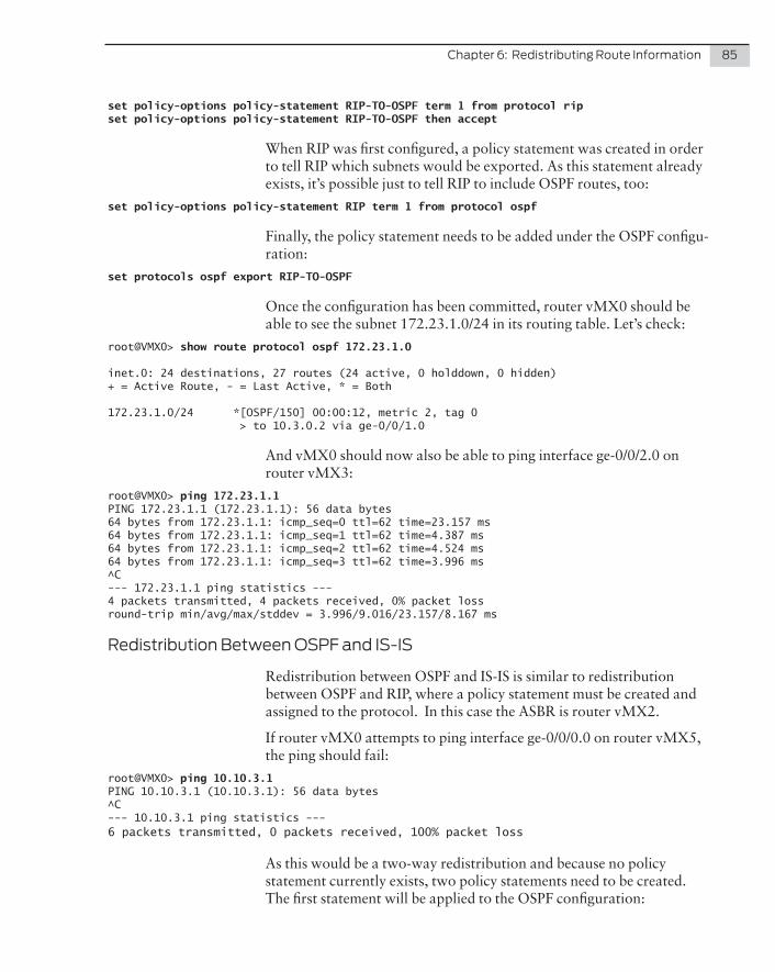
Chapter 6: Redistributing Route Information 85
set policy-options policy-statement RIP-TO-OSPF term 1 from protocol ripset policy-options policy-statement RIP-TO-OSPF then accept
When RIP was first configured, a policy statement was created in order to tell RIP which subnets would be exported. As this statement already exists, it’s possible just to tell RIP to include OSPF routes, too:
set policy-options policy-statement RIP term 1 from protocol ospf
Finally, the policy statement needs to be added under the OSPF configu-ration:
set protocols ospf export RIP-TO-OSPF
Once the configuration has been committed, router vMX0 should be able to see the subnet 172.23.1.0/24 in its routing table. Let’s check:
root@VMX0> show route protocol ospf 172.23.1.0
inet.0: 24 destinations, 27 routes (24 active, 0 holddown, 0 hidden)+ = Active Route, - = Last Active, * = Both
172.23.1.0/24 *[OSPF/150] 00:00:12, metric 2, tag 0 > to 10.3.0.2 via ge-0/0/1.0
And vMX0 should now also be able to ping interface ge-0/0/2.0 on router vMX3:
root@VMX0> ping 172.23.1.1PING 172.23.1.1 (172.23.1.1): 56 data bytes64 bytes from 172.23.1.1: icmp_seq=0 ttl=62 time=23.157 ms64 bytes from 172.23.1.1: icmp_seq=1 ttl=62 time=4.387 ms64 bytes from 172.23.1.1: icmp_seq=2 ttl=62 time=4.524 ms64 bytes from 172.23.1.1: icmp_seq=3 ttl=62 time=3.996 ms^C--- 172.23.1.1 ping statistics ---4 packets transmitted, 4 packets received, 0% packet lossround-trip min/avg/max/stddev = 3.996/9.016/23.157/8.167 ms
Redistribution Between OSPF and IS-IS
Redistribution between OSPF and IS-IS is similar to redistribution between OSPF and RIP, where a policy statement must be created and assigned to the protocol. In this case the ASBR is router vMX2.
If router vMX0 attempts to ping interface ge-0/0/0.0 on router vMX5, the ping should fail:
root@VMX0> ping 10.10.3.1PING 10.10.3.1 (10.10.3.1): 56 data bytes^C--- 10.10.3.1 ping statistics ---6 packets transmitted, 0 packets received, 100% packet loss
As this would be a two-way redistribution and because no policy statement currently exists, two policy statements need to be created. The first statement will be applied to the OSPF configuration:

86 Day One: Routing the Internet Protocol
set policy-options policy-statement ISIS-TO-OSPF term 1 from protocol isisset policy-options policy-statement ISIS-TO-OSPF then accept
And this second policy statement will be applied to the IS-IS configura-tion:
set policy-options policy-statement OSPF-TO-ISIS term 1 from protocol ospfset policy-options policy-statement OSPF-TO-ISIS then accept
These policy statements are then applied to the protocol configuration as follows:
set protocols ospf export ISIS-TO-OSPFset protocols isis export OSPF-TO-ISIS
Once things has been committed, router vMX0 should now be able to ping interface ge-0/0/0.0 on router vMX5:
root@VMX0> ping 10.10.3.1PING 10.10.3.1 (10.10.3.1): 56 data bytes64 bytes from 10.10.3.1: icmp_seq=0 ttl=63 time=4.817 ms64 bytes from 10.10.3.1: icmp_seq=1 ttl=63 time=4.841 ms64 bytes from 10.10.3.1: icmp_seq=2 ttl=63 time=5.747 ms64 bytes from 10.10.3.1: icmp_seq=3 ttl=63 time=4.142 ms64 bytes from 10.10.3.1: icmp_seq=4 ttl=63 time=6.485 ms^C--- 10.10.3.1 ping statistics ---5 packets transmitted, 5 packets received, 0% packet lossround-trip min/avg/max/stddev = 4.142/5.206/6.485/0.818 ms
Redistribution Between RIP and IS-IS
As with the redistribution between OSPF and RIP, it is perfectly accept-able to reuse the same policy statement RIP already uses. In this in-stance, however, rather than put IS-IS under the same term as RIP and direct, a second term has been created and IS-IS has been placed under this instead. As long as there is the then accept statement at the very end of the policy statement, then this will work, too. One reason to create this as a second term is to help keep it tidy, and to allow the administrator to see at a glance that a protocol is being redistributed.
This configuration will be applied to both vMX3 and vMX6 as these are both ASBRs between the RIP and IS-IS domains. The first command adds the second term to the policy statement RIP is currently using:
set policy-options policy-statement RIP term 2 from protocol isis
Once the RIP policy statement has been modified, a new policy state-ment that will be applied to the IS-IS configuration should be created:
set policy-options policy-statement RIP-TO-ISIS term 1 from protocol ripset policy-options policy-statement RIP-TO-ISIS then accept
Finally IS-IS is then told to use this policy statement:
set protocols isis export RIP-TO-ISIS

Chapter 6: Redistributing Route Information 87
In theory, even before the commands to redistribute between RIP and IS-IS were committed, all routers should have been able to see all subnets as routers vMX2 and vMX4 were redistributing between IS-IS and OSPF and between OSPF and RIP. What happens, however, if an interface goes down? By redistributing between these processes, too, the network should have full redundancy. To prove this, interface ge-0/0/0.0 on router vMX2 will be disabled.
First, if traceroute were to be run from vMX0 to router vMX5s inter-face in subnet 10.10.1.2, the packet should go via router vMX2 as this is the best path:
root@VMX0> traceroute 10.10.1.2traceroute to 10.10.1.2 (10.10.1.2), 30 hops max, 40 byte packets 1 10.2.0.3 (10.2.0.3) 2.813 ms 1.773 ms 1.238 ms 2 10.10.1.2 (10.10.1.2) 3.897 ms 3.536 ms 3.518 ms
The interface between vMX0 and vMX2 is then disabled by using the following command:
set interfaces ge-0/0/0.0 disable
After a brief pause to allow the route to be withdrawn, traceroute is run once more to the same address. This time the packet traverses routers vMX1, vMX4, vMX3, and vMX2:
root@VMX0> traceroute 10.10.1.2traceroute to 10.10.1.2 (10.10.1.2), 30 hops max, 40 byte packets 1 10.3.0.2 (10.3.0.2) 1.673 ms 1.557 ms 1.211 ms 2 10.5.0.2 (10.5.0.2) 1.958 ms 1.659 ms 2.345 ms 3 172.23.3.1 (172.23.3.1) 8.090 ms 2.908 ms 3.335 ms 4 10.10.2.1 (10.10.2.1) 7.119 ms 4.644 ms 5.151 ms 5 10.10.1.2 (10.10.1.2) 5.828 ms 5.396 ms 4.431 ms
Filtering Routes During Redistribution
The configuration covered in the previous section would, of course, redistribute every route between protocols, meaning every subnet was accessible from every part of the network. Imagine for a moment that this was not a desirable result and that there were some subnets you didn’t want to redistribute.
By utilizing the same policy statement, in addition to a prefix-list, it is possible to filter out individual subnets so that they aren’t redistributed. In this section, the subnet 172.23.1.0/24 will be filtered by the ASBRs so that routers vMX0 and vMX1 and the two VSRX firewalls will not be able to reach that subnet. Before this is done, however, router vMX0 should be checked to see if it does have reachability to that subnet:
root@VMX0> show route protocol ospf
inet.0: 25 destinations, 29 routes (25 active, 0 holddown, 0 hidden)+ = Active Route, - = Last Active, * = Both

88 Day One: Routing the Internet Protocol
10.4.0.0/24 *[OSPF/10] 00:14:00, metric 2000 > to 10.3.0.2 via ge-0/0/1.010.5.0.0/24 *[OSPF/10] 00:14:00, metric 2000 > to 10.3.0.2 via ge-0/0/1.010.10.1.0/24 *[OSPF/150] 00:13:09, metric 2, tag 0 > to 10.3.0.2 via ge-0/0/1.010.10.2.0/24 *[OSPF/150] 00:13:14, metric 2, tag 0 > to 10.3.0.2 via ge-0/0/1.010.10.3.0/24 *[OSPF/150] 00:12:48, metric 2, tag 0 > to 10.3.0.2 via ge-0/0/1.010.233.240.0/20 [OSPF/150] 00:13:14, metric 0, tag 0 > to 10.3.0.2 via ge-0/0/1.0172.23.1.0/24 *[OSPF/150] 00:13:14, metric 2, tag 0 > to 10.3.0.2 via ge-0/0/1.0172.23.3.0/24 *[OSPF/10] 00:13:14, metric 3000 > to 10.3.0.2 via ge-0/0/1.0172.23.7.0/24 *[OSPF/10] 00:13:14, metric 3000 > to 10.3.0.2 via ge-0/0/1.0192.168.1.0/24 *[OSPF/150] 00:13:14, metric 2, tag 0 > to 10.3.0.2 via ge-0/0/1.0192.168.1.1/32 *[OSPF/150] 00:13:09, metric 2, tag 0 > to 10.3.0.2 via ge-0/0/1.0192.168.1.2/32 *[OSPF/150] 00:13:14, metric 2, tag 0 > to 10.3.0.2 via ge-0/0/1.0192.168.1.3/32 *[OSPF/150] 00:12:48, metric 2, tag 0 > to 10.3.0.2 via ge-0/0/1.0192.168.1.4/32 *[OSPF/150] 00:12:08, metric 2, tag 0 > to 10.3.0.2 via ge-0/0/1.0224.0.0.5/32 *[OSPF/10] 00:15:29, metric 1 MultiRecv
In the previous sections, a policy statement was created and assigned to the OSPF configuration. The first router these changes will be made to is vMX2. The configuration of the existing policy statement is as follows:
policy-statement ISIS-TO-OSPF { term 1 { from { protocol isis; } then accept;}
This policy statement can be easily modified by adding extra “terms.” Before this is done, however, a prefix list needs to be created that will identity which subnets are to be filtered. The name of this prefix list will be ONESEVENTWOTWENTYTHREEONE and it will match the subnet 172.23.1.0/24:
set policy-options prefix-list ONESEVENTWOTWENTYTHREEONE 172.23.1.0/24
Now that the prefix list has been created, it can be added to the policy statement. Policy statements operate from the top down. As soon as the policy statement finds a match, it stops processing, and if it doesn’t

Chapter 6: Redistributing Route Information 89
find a match then it automatically rejects. In this case, if the filter was applied to the next “term” then the policy statement will still allow this route, through, and therefore the prefix list needs to be applied to Term 1, then within Term 1 a reject will be set.
NOTE There are in fact two ways of specifying which routes should be filtered, the first is using the prefix-list as described here, and the second is using a route-filter, which will be covered in Chapter 9, where routes will be filtered and summarized instead:
set policy-options policy-statement ISIS-TO-OSPF term 1 from prefix-list ONESEVENTWOTWENTYTHREEONEset policy-options policy-statement ISIS-TO-OSPF term 1 then reject
If this were to be committed now, this policy would reject all routes because of the implicit reject, therefore a second term needs to be created that matches just the protocol. The accept term already at the end of the policy statement will ensure that routes other than the one filtered in Term 1, are now accepted:
set policy-options policy-statement ISIS-TO-OSPF term 2 from protocol isis
Once this is committed, router vMX0 will be able to reach this subnet, because there are two ASBRs. So these filters need to be applied to vMX4, too. In this case, the filter needs to be applied on the policy statement that redistributes RIP into OSPF. The existing policy state-ment is configured as follows:
policy-statement RIP-TO-OSPF { term 1 { from { protocol rip; } then accept;}
The first thing that should be done is to create the prefix list. In this case it will be given the same name as on router vMX2:
set policy-options prefix-list ONESEVENTWOTWENTYTHREEONE 172.23.1.0/24
And, as before, this should be added to Term 1 and a reject should be applied:
set policy-options policy-statement RIP-TO-OSPF term 1 from prefix-list ONESEVENTWOTWENTYTHREEONEset policy-options policy-statement RIP-TO-OSPF term 1 then reject
Finally, a second term needs to be created so that the other routes are accepted:
set policy-options policy-statement RIP-TO-OSPF term 2 from protocol rip

90 Day One: Routing the Internet Protocol
If vMX0 starts to ping vMX3’s ge-0/0/2.0 interface while the configu-ration is committed to router vMX4, you should see that the route is very quickly withdrawn by OSPF. In this case, the Junos OS warns us that there was no route to the host:
root@VMX0> ping 172.23.1.1PING 172.23.1.1 (172.23.1.1): 56 data bytes64 bytes from 172.23.1.1: icmp_seq=0 ttl=62 time=10.478 ms64 bytes from 172.23.1.1: icmp_seq=10 ttl=62 time=5.307 ms64 bytes from 172.23.1.1: icmp_seq=11 ttl=62 time=9.757 msping: sendto: No route to hostping: sendto: No route to hostping: sendto: No route to host
As a final check, just by looking at the routing table, it should be apparent that this route has disappeared, meaning the filter was successful:
root@VMX0> show route protocol ospf | match 172.23172.23.3.0/24 *[OSPF/10] 00:20:21, metric 3000172.23.7.0/24 *[OSPF/10] 00:20:21, metric 3000
Summary
While running a single protocol on a LAN is ideal, this is not always possible and as such this chapter has demonstrated that it is possible to run two, three, or even four routing protocols on a LAN at the same time should the need arise.
Aside from being used during an acquisition or merger, redistribution is typically used when a corporate LAN grows beyond its existing routing protocol. An administrator can enable the new routing protocol on a router by router basis and redistribute between the new and the old protocol until the migration is complete.
Junos is ideal in this case as the administrator has an easy means to rollback the configuration should something go wrong during a migration. In addition the Junos OS runs each protocol in its own process thereby protecting the network device should something happen to one of the processes, this means the network largely remains accessible.
The next chapter covers the most scalable protocol available on any network today. The scalability is such that it is capable of advertising almost every single subnet that exists in the world, with the exception of those in the private address ranges. This protocol is BGP.

The previous chapters in this Day One book have explored interior gateway protocols (IGPs). Let’s now move on to exterior gateway protocols (EGPs).
So much has been written already about BGP that it is hard to add a unique introduction to one of world’s most popular protocols. It literally runs the world’s networks!
NOTE Do not confuse EGP with the 1980s EGP3 that was defined in RFC 827. EGP in this book refers to BGP4 (Border Gateway Protocol).
BGP4 is a routing protocol that operates between networks that are under different administrative control. This is what makes BGP4 an exterior gateway protocol as it operates between Autonomous Systems (ASs).
BGP is an exterior gateway protocol that allows the exchange of routing information between routers in different autonomous systems (ASs). Routing information includes the complete route to each destination. BGP uses this information to maintain a Routing Informa-tion Base (RIB), which allows it to remove routing loops and to enforce policy decisions at an AS level.
Chapter 7
Border Gateway Protcol (BGP)
Border Gateway Protocol (BGP) is a standardized exterior gateway protocol designed to exchange routing and reachability information between autonomous systems (ASs) on the Internet .
https://en .wikipedia .org/wiki/Border_Gateway_Protocol .

92 Day One: Routing the Internet Protocol
BGP allows for policy-based routing. You can use routing policies to choose among multiple paths to a destination and to control the redistribution of routing information.
An AS is defined as a group of IP networks operated by one or more network operators that has a single, clearly defined routing policy.
If you look back at Chapter 2, Table 2.2, you can see that BGP (both iBGP and eBGP) is a path vector routing protocol that uses the unique-ness of AS numbers to help detect any loops. BGP uses additional attributes to describe the path to prefixes, also known as reachability information. These attributes are discussed later in this chapter.
One of the main differences of BGP as a routing protocol compared to other IGPs in this book is that BGP uses the Transmission Control Protocol (TCP) for its transporting reliability. This means that there is no need for periodic route updates – quite handy since the current BGP Global IPv4 routing table is ~542,000 prefixes! With the lack of periodic updates, BGP still needs to confirm that other ASs are still reachable and functional. This is resolved by the use of keepalive packets.
Now, before drilling down into the Junos OS examples, let’s first discuss routing attributes.
BGP Route Attributes
BGP uses additional attributes and route reachability to describe the path to prefixes. This is referred to as Next Layer Reachability Infor-mation (NLRI).
Below are the categories into which all BGP route attributes fall. There are also examples of BGP path attributes on each category, as well as a short explanation:
� Well-known mandatory: Must be present in all update messages and must be supported by all BGP speakers. AS Path, Next-hop, Origin.
� Well-known discretionary: May be present in update messages and must be supported by all BGP speakers. Local Preference, Atomic Aggregate.
� Optional transitive: May not be recognized by all BGP speakers. If not recognized it is still expected to be propagated to other neighbors. Community, Aggregator.
The Transmission Control Protocol (TCP) is a core protocol of the Internet Protocol Suite . It originated in the initial network implementation in which it complemented the Internet Protocol (IP) .
https://en .wikipedia .org/wiki/Transmission_Control_Protocol .
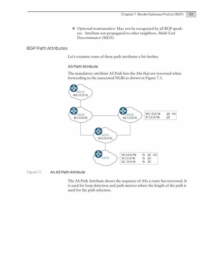
Chapter 7: Border Gateway Protcol (BGP) 93
� Optional nontransitive: May not be recognized by all BGP speak-ers. Attribute not propagated to other neighbors. Multi Exit Descriminator (MED).
BGP Path Attributes
Let’s examine some of these path attributes a bit further.
AS Path Attribute
The mandatory attribute AS Path lists the ASs that are traversed when forwarding to the associated NLRI as shown in Figure 7.1.
Figure 7.1 An AS Path Attribute
The AS Path Attribute shows the sequence of ASs a route has traversed. It is used for loop detection and path metrics where the length of the path is used for the path selection.

94 Day One: Routing the Internet Protocol
Loop Detection
Figure 7.2 Loop Detection Attribute
You can see here in Figure 7.2 that 92.1.0.0/16 is not accepted by AS30 due it having AS40 in its path.
Next Hop
Figure 7.3 Next Hop Attribute

Chapter 7: Border Gateway Protcol (BGP) 95
The next hop AS attribute shows the IP address to reach the next AS. From the viewpoint of AS15, you can see the following:
root@AS15> show route protocol bgp
inet.0: 9 destinations, 10 routes (9 active, 0 holddown, 0 hidden)+ = Active Route, - = Last Active, * = Both
90.1.0.0/16 *[BGP/170] 00:40:49, localpref 100 AS path: 20 40 I, validation-state: unverified > to 10.0.0.2 via ge-0/0/0.0 [BGP/170] 00:40:49, localpref 100 AS path: 30 40 I, validation-state: unverified > to 10.0.0.6 via ge-0/0/1.091.1.0.0/16 *[BGP/170] 00:49:35, localpref 100 AS path: 20 I, validation-state: unverified > to 10.0.0.2 via ge-0/0/0.092.1.0.0/16 *[BGP/170] 00:50:10, localpref 100 AS path: 30 I, validation-state: unverified > to 10.0.0.6 via ge-0/0/1.0
So AS15 can see 90.1.0.0/ via two paths. One path via 10.0.0.2, which is AS20, and the other path via 10.0.0.6, which is AS30.
The next-hop attribute is well known and mandatory in BGP.
Local Preference
The local preference attribute is used to advertise to iBGP neighbors on how to leave their AS. It is a well-known discretionary attribute and is kept within the AS. The higher the local preference the more desirable the path.
Origin
The origin code is used to identify the original source of a route being learned. It can be one of the following:
� I – IGP
� E – EGP
� ? – Unknown/Incomplete
90.1.0.0/16 *[BGP/170] 00:40:49, localpref 100 AS path: 20 40 I, validation-state: unverified > to 10.0.0.2 via ge-0/0/0.0
A BGP speaker prefers origins in the following order: IGP / EGP / Unknown/Incomplete. Origin is a well known mandatory attribute.

96 Day One: Routing the Internet Protocol
Multi Exit Discriminator
The multi exit discriminator (MED) is an optional non-transitive attribute and some BGP speakers may not understand or even use the attribute. MED is also kept within the AS it was advertised to and will not transit any further. Here’s an example:
root@AS20> show route protocol bgp
inet.0: 9 destinations, 10 routes (9 active, 0 holddown, 0 hidden)+ = Active Route, - = Last Active, * = Both
90.1.0.0/16 *[BGP/170] 00:01:07, MED 10, localpref 100 AS path: 40 I, validation-state: unverified > to 10.0.0.10 via ge-0/0/0.0
The lower the MED the more preferred the path, should all other decisions with BGP path selection process be equal (more on BGP path selection next).
Community
BGP communities allow for the tagging of multiple routes that may share one or more characteristics. These tags can be used to allow upstream devices to apply specific routing policies within their AS.
The common format is LOCAL-AS:xx, where xx is represented as two 16 bit integers as per RFC1998. Community is an optional transitive attribute.
BGP Path Selection Tutorial
The Junos OS BGP path selection algorithm is slightly different from other vendors (who all have their own slant of path selection). This book only describes the Juniper path selection process so as not to muddy the waters.
NOTE For interop issues, you should consult the documentation of your device’s vendor.
When a BGP router is presented with a prefix that has more than one route to it, the Junos OS route selection process is started and it operates on the following logic:
1. Can the next hop be resolved?
2. Prefers the path with the highest local preference
3. Prefers the path with the shortest AS path length
4. Prefers the path with the lowest origin value

Chapter 7: Border Gateway Protcol (BGP) 97
5. Prefers the path with lower MED value
6. Prefers paths learned by eBGP over iBGP
7. Prefers paths with lowest IGP metric
8. Prefers paths with shortest cluster length
9. Prefers routes from peer with lowest router ID
10. Prefers routes from peer with lowest peer ID
The last two points can be removed if you activate multipath. Enabling the multipath option allows routes for the same prefix that have passed the first eight steps to be installed onto the route table.
MORE? For more on the multipath option, see the Juniper TechLibrary: http://www.juniper.net/techpubs/en_US/junos12.1/topics/reference/configura-tion-statement/multipath-edit-protocols-bgp.html.
Having digested all that, let’s take a look at BGP path selection using the topology shown in Figure 7.4.
Figure 7.4 BGP Path Selection Example
Figure 7.4 has four routers within AS15 and two external ASs, 65500, and 65501, announcing 192.0.2.0/24, and 203.0.113.0/24, respective-ly. OSPF is running between them and the loopbacks are also an-nounced.
There is a full mesh of iBGP sessions between all four routers within AS15. To calculate the amount of iBGP sessions you need a full mesh that uses the following calculation: N(N-1)/2 and applied to the above 4(4-1)/2 = 6.
So let’s have a look at R3 and R4 to see the routes that the external ASs are announcing:

98 Day One: Routing the Internet Protocol
root@R3> show bgp summary Groups: 2 Peers: 5 Down peers: 0Table Tot Paths Act Paths Suppressed History Damp State Pendinginet.0 6 2 0 0 0 0Peer AS InPkt OutPkt OutQ Flaps Last Up/Dwn State|#Active/Received/Accepted/Damped...90.1.0.1 15 227 227 0 0 1:40:57 0/0/0/0 0/0/0/091.1.0.1 15 176 177 0 0 1:19:04 0/0/0/0 0/0/0/092.1.0.1 15 187 186 0 0 1:23:11 0/2/2/0 0/0/0/0198.51.100.6 65500 56 53 0 0 23:01 1/2/2/0 0/0/0/0198.51.100.10 65501 96 96 0 0 41:42 1/2/2/0 0/0/0/0
From R3 you can see that AS 65500 and 65001 are both sending two routes that have been accepted but only one route from each AS has been made active. You can also see the two routes via the iBGP session with 92.1.0.1, but neither are the active routes. This is due to the best path selection preferring eBGP over iBGP in Step 6 of the selection process. Now, let’s have a look at why only one route from each session is active:
root@R3> show route receive-protocol bgp 198.51.100.6
inet.0: 20 destinations, 25 routes (20 active, 0 holddown, 2 hidden) Prefix Nexthop MED Lclpref AS path 192.0.2.0/24 198.51.100.6 65500 65501 I* 203.0.113.0/24 198.51.100.6 65500 I
root@R3> show route receive-protocol bgp 198.51.100.10
inet.0: 20 destinations, 25 routes (20 active, 0 holddown, 2 hidden) Prefix Nexthop MED Lclpref AS path* 192.0.2.0/24 198.51.100.10 65501 I 203.0.113.0/24 198.51.100.10 65501 65500 I
If you look closely you can see that both ASs are sending 192.0.2.0/24 and 203.0.113.0/24, but only one route is selected as active (denoted by the *). If you also look at the AS Path you can see that each external AS is announcing their locally originated route plus the other AS’s locally originated route. If you look back at Figure 7.3 you can see where the connection to each AS is, and you can see R3 has direct connections to each external AS.
This means that in the BGP best path selection process this made it Step 3 (prefers the path with the shortest AS Path length). It makes good sense, as there would be no point getting to 203.0.113.0/24 via 65501 when you can see it directly from 65500, and the same is true of 192.0.2.0/24 being seen via 65500 when you can see it directly via 65501. Why add an extra AS to traverse!
Let’s have a look at R4:

Chapter 7: Border Gateway Protcol (BGP) 99
root@R4> show bgp summary Groups: 2 Peers: 4 Down peers: 0Table Tot Paths Act Paths Suppressed History Damp State Pendinginet.0 4 2 0 0 0 0Peer AS InPkt OutPkt OutQ Flaps Last Up/Dwn State|#Active/Received/Accepted/Damped...90.1.0.1 15 253 256 0 0 1:54:01 0/0/0/0 0/0/0/091.1.0.1 15 246 247 0 0 1:50:45 0/0/0/0 0/0/0/093.1.0.1 15 253 254 0 0 1:53:53 0/2/2/0 0/0/0/0198.51.100.1 65500 103 102 0 0 45:07 2/2/2/0 0/0/0/0
Now in this output you can see that R4 is receiving two routes (bold-face): from iBGP (AS15) and eBGP (AS65500). You already know that eBGP is preferred over iBGP, so it makes sense that the active routes (routes installed to the Forwarding Information BASW – FIB) are installed from the routes accepted from AS6500. Let’s have a look at the routes learned from AS65500:
root@R4> show route receive-protocol bgp 198.51.100.1
inet.0: 15 destinations, 17 routes (15 active, 0 holddown, 2 hidden) Prefix Nexthop MED Lclpref AS path* 192.0.2.0/24 198.51.100.1 65500 65501 I* 203.0.113.0/24 198.51.100.1 65500 I
You can see here that R4 has received and accepted the two routes and has made them active in the FIB, which is great. As R4 only has one external eBGP connection, you are seeing both routes via AS65500 with 192.0.2.0/24 transiting through to AS65501.
So now, both the eBGP facing routers (R3 and R4) receive the same routes, and since there is a full mesh iBGP setup between all the routers in AS15, they should all be able to see the two external prefixes. Or can they? Let’s have a look at R2 to confirm:
root@R2> show bgp summary Groups: 1 Peers: 3 Down peers: 0Table Tot Paths Act Paths Suppressed History Damp State Pendinginet.0 4 0 0 0 0 0Peer AS InPkt OutPkt OutQ Flaps Last Up/Dwn State|#Active/Received/Accepted/Damped...90.1.0.1 15 325 326 0 0 2:26:22 0/0/0/0 0/0/0/092.1.0.1 15 286 286 0 0 2:08:35 0/2/2/0 0/0/0/093.1.0.1 15 283 283 0 0 2:07:36 0/2/2/0 0/0/0/0
Here, both R3 and R4 have sent two routes, which have been received and accepted, but they haven’t become active. Let’s do some debugging to see why, starting at R2:
root@R2> show route receive-protocol bgp 92.1.0.1
inet.0: 13 destinations, 15 routes (11 active, 0 holddown, 4 hidden)

100 Day One: Routing the Internet Protocol
Hmm, it’s not showing us any routes, but from the output (boldface) you can see that four routes are hidden. Could these be the two routes from R3 and from R4? Let’s investigate:
root@R2> show route receive-protocol bgp 92.1.0.1 hidden
inet.0: 13 destinations, 15 routes (11 active, 0 holddown, 4 hidden) Prefix Nexthop MED Lclpref AS path 192.0.2.0/24 198.51.100.1 100 65500 65501 I 203.0.113.0/24 198.51.100.1 100 65500 I
root@R2> show route receive-protocol bgp 93.1.0.1 hidden
inet.0: 13 destinations, 15 routes (11 active, 0 holddown, 4 hidden) Prefix Nexthop MED Lclpref AS path 192.0.2.0/24 198.51.100.10 100 65501 I 203.0.113.0/24 198.51.100.6 100 65500 I
The missing routes are found, but why are they hidden? The AS paths look correct, and the next hop and the Origin attributes all look okay. Let’s look at one of the hidden routes in a bit more detail using the extensive option:
root@R2> show route 192.0.2.0/24 hidden extensive
inet.0: 13 destinations, 15 routes (11 active, 0 holddown, 4 hidden)192.0.2.0/24 (2 entries, 0 announced) BGP Preference: 170/-101 Next hop type: Unusable Address: 0x92854a4 Next-hop reference count: 4 State: <Hidden Int Ext> Local AS: 15 Peer AS: 15 Age: 1:12:13 Validation State: unverified Task: BGP_15.92.1.0.1+179 AS path: 65500 65501 I Aggregator: 65501 192.0.2.1 Accepted Localpref: 100 Router ID: 92.1.0.1 Indirect next hops: 1 Protocol next hop: 198.51.100.1 Indirect next hop: 0x0 - INH Session ID: 0x0 BGP Preference: 170/-101 Next hop type: Unusable Address: 0x92854a4 Next-hop reference count: 4 State: <Hidden Int Ext> Local AS: 15 Peer AS: 15 Age: 1:39:30 Validation State: unverified Task: BGP_15.93.1.0.1+179 AS path: 65501 I Aggregator: 65501 192.0.2.1 Accepted Localpref: 100 Router ID: 93.1.0.1 Indirect next hops: 1 Protocol next hop: 198.51.100.10 Indirect next hop: 0x0 - INH Session ID: 0x0

Chapter 7: Border Gateway Protcol (BGP) 101
So you can see the routes from both R3 and R4, but both are saying the next hop is unusable!? Let’s double-check this:
root@R2> show route 198.51.100.1
root@R2> show route 198.51.100.10
root@R2>
The next hops that both R3 and R4 are advertising are not in the routing table. How do you fix this? Let’s jump back to R4 and see what can be done:
root@R4> show route 198.51.100.1
inet.0: 15 destinations, 17 routes (15 active, 0 holddown, 2 hidden)+ = Active Route, - = Last Active, * = Both
198.51.100.0/30 *[Direct/0] 01:32:08 > via ge-0/0/2.0
Here, R4 does have a route to 198.51.100.1. That makes sense, as both routes are active on this router, allowing them to be announced back to R2. So how does R2, and presumably all the other routers in AS15, know about this directly connected interface and also the two directly connected interfaces on R3? Static routes can be added (remember Chapter 1?) across all the routers in AS15 but this seems a bit cumbersome and not very scalable. Let’s look at a routing protocol, like OSPF, and passively add the interface into OSPF and see what happens on R2:
[edit]root@R4# set protocols ospf area 0.0.0.0 interface ge-0/0/2.0
[edit]root@R4# commit commit complete
Now to check out R2:
[root@R2> show bgp summary Groups: 1 Peers: 3 Down peers: 0Table Tot Paths Act Paths Suppressed History Damp State Pendinginet.0 4 2 0 0 0 0Peer AS InPkt OutPkt OutQ Flaps Last Up/Dwn State|#Active/Received/Accepted/Damped...90.1.0.1 15 394 395 0 0 2:57:53 0/0/0/0 0/0/0/092.1.0.1 15 354 355 0 0 2:40:06 2/2/2/0 0/0/0/093.1.0.1 15 351 352 0 0 2:39:07 0/2/2/ 0/0/0/0
root@R2> show route receive-protocol bgp 92.1.0.1
inet.0: 14 destinations, 16 routes (14 active, 0 holddown, 2 hidden) Prefix Nexthop MED Lclpref AS path* 192.0.2.0/24 198.51.100.1 100 65500 65501 I* 203.0.113.0/24 198.51.100.1 100 65500 I

102 Day One: Routing the Internet Protocol
Great! Both routes are now active but two routes are still hidden and it still needs the external interfaces on R3 added into OSPF. Let’s do this and then see how this affects R2:
root@R2> show bgp summary Groups: 1 Peers: 3 Down peers: 0Table Tot Paths Act Paths Suppressed History Damp State Pendinginet.0 3 2 0 0 0 0Peer AS InPkt OutPkt OutQ Flaps Last Up/Dwn State|#Active/Received/Accepted/Damped...90.1.0.1 15 405 406 0 0 3:02:48 0/0/0/0 0/0/0/092.1.0.1 15 366 366 0 0 2:45:01 0/1/1/0 0/0/0/093.1.0.1 15 362 363 0 0 2:44:02 2/2/2/0 0/0/0/0
Fantastic! The active routes from R3 can be seen now, which makes sense because looking at the BGP best path selection steps you can see that they have been selected because:
� 192.0.2.0/24 is selected as active from R3 because it is a shorter AS Path length than R4.
� 203.0.113.0/24 is selected as active from R3 because it is a lower IGP metric from R2 to R3 than R2 to R4.
The more careful reader may have spotted that there is only receiving one route from R4 instead of an earlier two. Why would that be? Let’s have a look back on R4:
root@R4> show bgp summary Groups: 2 Peers: 4 Down peers: 0Table Tot Paths Act Paths Suppressed History Damp State Pendinginet.0 4 2 0 0 0 0Peer AS InPkt OutPkt OutQ Flaps Last Up/Dwn State|#Active/Received/Accepted/Damped...90.1.0.1 15 1886 1887 0 1 10:41:22 0/0/0/0 0/0/0/091.1.0.1 15 1886 1888 0 1 13:07:38 0/0/0/0 0/0/0/093.1.0.1 15 1886 1889 0 0 14:14:25 1/2/2/0 0/0/0/0198.51.100.2 65500 89 88 0 0 38:35 1/2/2/0 0/0/0/0
You can see that there is one learned route from AS65500 and one from our iBGP neighbor, R3. Let’s have a look at the routes and why there is one active from each peer:
root@R4> show route protocol bgp
inet.0: 19 destinations, 21 routes (19 active, 0 holddown, 0 hidden)+ = Active Route, - = Last Active, * = Both
192.0.2.0/24 *[BGP/170] 01:08:53, localpref 100, from 93.1.0.1 AS path: 65501 I, validation-state: unverified > to 10.0.0.5 via ge-0/0/2.0 [BGP/170] 01:08:49, localpref 100 AS path: 65500 65501 I, validation-state: unverified > to 198.51.100.2 via ge-0/0/3.0203.0.113.0/24 *[BGP/170] 01:25:59, localpref 100 AS path: 65500 I, validation-state: unverified > to 198.51.100.2 via ge-0/0/3.0

Chapter 7: Border Gateway Protcol (BGP) 103
[BGP/170] 01:26:45, localpref 100, from 93.1.0.1 AS path: 65500 I, validation-state: unverified > to 10.0.0.5 via ge-0/0/2.0
Here you can see that each route has two paths. BGP best path has selected both active routes due to their shortest AS Path length. However, iBGP does not prepend its own AS when making the calcula-tion, and that is why 192.02.0/24 is preferred via 65501 with the next hop being R3.
Now does this explain why R4 is only sending one route to R2 or doesn’t it? Let’s investigate iBGP to find out.
iBGP
At the beginning of this chapter eBGP was noted as external and iBGP as being internal. External peers (according to peers within an AS) establish links via eBGP. The router then takes these routes and advertises them internally within the AS with other BGP-speaking peers with iBGP.
One of the fundamental differences between iBGP and eBGP is that to avoid routing loops iBGP does not advertise routes learned from other iBGP neighbors.
For this reason, BGP cannot propagate routes throughout an AS by passing them from one router to another. Instead, BGP requires that all internal peers be fully meshed so that any route advertised by one router is advertised to all peers within the AS.
And this explains why R2 is only seeing one prefix from R4 because it has learned one route from eBGP (which is advertised to R2) and one route from iBGP (which is not advertised to avoid routing loops). This means that our topology is working as expected.
Scaling iBGP
The topology that has been used in the AS is a full mesh BGP that is manageable, but what if there were fifty routers within the AS? Using the calculation, you can see that fifty routers would require 50(50-1)/2=1225 BGP peering sessions. That’s a lot of time and effort to put into the network to build it full mesh! What if there was a way to scale the amount of routers within your network but not be held up by setting up a full mesh network?
MORE? Thankfully there are two ways to scale your iBGP: route reflectors and confederations. The implementation of these two methodologies is outside the scope of this Day One book, but further information can
Fully Meshed: A mesh network whose nodes are all connected to each other is a fully connected network .
https://en .wikipedia .org/wiki/Mesh_networking .

104 Day One: Routing the Internet Protocol
be found at the Juniper TechLibrary: http://www.juniper.net/documen-tation/en_US/junos15.1/topics/concept/routing-protocol-bgp-security-route-reflector-understanding.html; and at, http://www.juniper.net/documentation/en_US/junos13.1/topics/topic-map/bgp-confedera-tions.html
Let’s look at scaling BGP and how to resolve the next-hop issue by adding external links. Is this really scalable by adding all these link subnets to our IGP? Probably not, so let’s see what we can do about that.
The reason the external links were added to our IGP was to activate routes within our AS that couldn’t resolve the next hop. A quick reminder is here:
root@R2> show route 192.0.2.0/24 hidden extensive
inet.0: 13 destinations, 15 routes (11 active, 0 holddown, 4 hidden)192.0.2.0/24 (2 entries, 0 announced) BGP Preference: 170/-101 Next hop type: Unusable Address: 0x92854a4 Next-hop reference count: 4 State: <Hidden Int Ext> Local AS: 15 Peer AS: 15 Age: 1:12:13 Validation State: unverified Task: BGP_15.92.1.0.1+179 AS path: 65500 65501 I Aggregator: 65501 192.0.2.1 Accepted Localpref: 100 Router ID: 92.1.0.1 Indirect next hops: 1 Protocol next hop: 198.51.100.1 Indirect next hop: 0x0 - INH Session ID: 0x0 BGP Preference: 170/-101 Next hop type: Unusable Address: 0x92854a4 Next-hop reference count: 4 State: <Hidden Int Ext> Local AS: 15 Peer AS: 15 Age: 1:39:30 Validation State: unverified Task: BGP_15.93.1.0.1+179 AS path: 65501 I Aggregator: 65501 192.0.2.1 Accepted Localpref: 100 Router ID: 93.1.0.1 Indirect next hops: 1 Protocol next hop: 198.51.100.10 Indirect next hop: 0x0 - INH Session ID: 0x0
So the next hop to 198.51.100.1 and 198.51.100.10 is unusable because it’s not in the IGP, so what can you do to resolve this? Let’s have a look at R2 and show OSPF:

Chapter 7: Border Gateway Protcol (BGP) 105
root@R2> show route protocol ospf inet.0: 18 destinations, 19 routes (18 active, 0 holddown, 0 hidden)+ = Active Route, - = Last Active, * = Both
10.0.0.4/30 *[OSPF/10] 20:09:34, metric 2 > to 10.0.0.2 via ge-0/0/2.010.0.0.12/30 *[OSPF/10] 02:26:11, metric 2 > to 10.0.0.9 via ge-0/0/1.090.1.0.1/32 *[OSPF/10] 02:26:11, metric 1 > to 10.0.0.9 via ge-0/0/1.092.1.0.1/32 *[OSPF/10] 02:26:11, metric 2 > to 10.0.0.9 via ge-0/0/1.0 to 10.0.0.2 via ge-0/0/2.093.1.0.1/32 *[OSPF/10] 20:09:34, metric 1 > to 10.0.0.2 via ge-0/0/2.0198.51.100.0/30 *[OSPF/10] 02:26:11, metric 3 > to 10.0.0.9 via ge-0/0/1.0 to 10.0.0.2 via ge-0/0/2.0198.51.100.4/30 *[OSPF/10] 09:35:13, metric 2 > to 10.0.0.2 via ge-0/0/2.0198.51.100.8/30 *[OSPF/10] 09:35:13, metric 2 > to 10.0.0.2 via ge-0/0/2.0224.0.0.5/32 *[OSPF/10] 23:44:42, metric 1 MultiRecv
From R2’s output you can see the link subnets between OSPF neigh-bors and you can also see the loopback interfaces of the other routers within the AS, which is handy because they are the IPs that we are establishing our iBGP sessions to and from. What if the next-hop addresses could be changed to that of the router which learned the route? That would allow the AS to scale without adding additional routes into the IGP. Let’s have a go!
First, roll back the changes on R3 and R4 and see things are back to accepting routes but not activating them from R2:
root@R2> show bgp summary Groups: 1 Peers: 3 Down peers: 0Table Tot Paths Act Paths Suppressed History Damp State Pendinginet.0 4 0 0 0 0 0Peer AS InPkt OutPkt OutQ Flaps Last Up/Dwn State|#Active/Received/Accepted/Damped...90.1.0.1 15 3190 3192 0 0 1d 0:04:53 0/0/0/0 0/0/0/092.1.0.1 15 3043 3046 0 1 22:58:10 0/2/2/0 0/0/0/093.1.0.1 15 3183 3194 0 0 1d 0:05:02 0/2/2/0 0/0/0/0
That takes us back to an earlier point in this chapter, before adding the interfaces to OSPF, so let’s jump on to R4 and see how to set the eBGP learned routes to be advertised to our iBGP neighbors with the next hop of R4’s loopback interface. It may sound daunting but it’s really simple because from the standpoint of R4, it is exporting routes to the other iBGP neighbors. So let’s create a policy and apply it as an export to our iBGP neighbors:

106 Day One: Routing the Internet Protocol
root@R4# set policy-options policy-statement NEXT-HOP-SELF then accept next-hop self
[edit]root@R4# set protocols bgp group internal export NEXT-HOP-SELF
[edit]root@R2# commit commit complete
[edit]root@R4# show protocols bgp group internal type internal;local-address 92.1.0.1;export NEXT-HOP-SELF;peer-as 15;local-as 15;neighbor 90.1.0.1 { description R1;}neighbor 91.1.0.1 { description R2;}neighbor 93.1.0.1 { description R3;}
And let’s see if the desired result is on R2:
root@R2> show bgp summary Groups: 1 Peers: 3 Down peers: 0Table Tot Paths Act Paths Suppressed History Damp State Pendinginet.0 4 2 0 0 0 0Peer AS InPkt OutPkt OutQ Flaps Last Up/Dwn State|#Active/Received/Accepted/Damped...90.1.0.1 15 3222 3228 0 0 1d 0:18:57 0/0/0/0 0/0/0/092.1.0.1 15 3076 3081 0 1 23:12:14 2/2/2/0 0/0/0/093.1.0.1 15 3214 3230 0 0 1d 0:19:06 0/2/2/0 0/0/0/0
Looking good so far. Let’s have a look at the routes received:
root@R2> show route receive-protocol bgp 92.1.0.1 detail
inet.0: 15 destinations, 17 routes (15 active, 0 holddown, 2 hidden)* 192.0.2.0/24 (2 entries, 1 announced) Accepted Nexthop: 92.1.0.1 Localpref: 100 AS path: 65500 65501 I Aggregator: 65501 192.0.2.1
* 203.0.113.0/24 (2 entries, 1 announced) Accepted Nexthop: 92.1.0.1 Localpref: 100 AS path: 65500 I Aggregator: 65500 203.0.113.1
Fantastic! You can see that the next-hop address for both routes is now the loopback of R4. All that’s left to do is add the next-hop policy to R3 and you should be back to having an active route from R4 and R3 on router R2:

Chapter 7: Border Gateway Protcol (BGP) 107
root@R2> show bgp summary Groups: 1 Peers: 3 Down peers: 0Table Tot Paths Act Paths Suppressed History Damp State Pendinginet.0 3 2 0 0 0 0Peer AS InPkt OutPkt OutQ Flaps Last Up/Dwn State|#Active/Received/Accepted/Damped...90.1.0.1 15 3248 3255 0 0 1d 0:31:05 0/0/0/0 0/0/0/092.1.0.1 15 3104 3108 0 1 23:24:22 0/1/1/0 0/0/0/093.1.0.1 15 3247 3257 0 0 1d 0:31:14 2/2/2/0 0/0/0/0
Awesome! You are now seeing one route received from R4 and two routes received and activated from R2, which is the same as when there were the two external links in OSPF, but this time there are two less /30 link subnets in the IGP!
From this last example you can see that a routing policy was used to achieve our objective. Routing policies can be very powerful and can help us achieve many objectives, so let’s look at them further.
BGP Routing Policy
Junos routing policy is both fast and granular so it could have a Day One book to itself. In the meantime, this chapter covers some basics to give you a taste of what it can do. Further exploration is advised to the reader.
Let’s continue from the previous example where a next-hop self policy was used to affect routing decisions within the AS. But now let’s expand on that further and have a look at manipulating both ingress and egress traffic. To do this, look at the import policy to affect routing decisions on how traffic exits our AS and also the export policies that affect routing decisions on traffic destined to our AS. Figure 7.5 repeats Figure 7.4 for your convenience.
Figure 7.5 This Section’s Network Topology

108 Day One: Routing the Internet Protocol
The network AS15 has been assigned 10.0.0.0/24 by the Acme Inernet Registry, hurrah! Let’s announce it to our transit providers!
On R3 and R4 create an export policy as follows:
root@R3# show | compare [edit policy-options]+ policy-statement ANNOUNCE-OUR-RANGE {+ term announce-aggregate-route {+ from {+ protocol aggregate;+ route-filter 10.0.0.0/24 exact;+ }+ then accept;+ }+ }
Let’s have a look at our BGP group to see what it looks like now:
root@R3# show protocols bgp group external type external;log-updown;export ANNOUNCE-OUR-RANGE;local-as 15;neighbor 198.51.100.10 { peer-as 65501;}neighbor 198.51.100.6 { peer-as 65500;}
Great. Let’s see if it is announcing to the transits:
root@R3> show route advertising-protocol bgp 198.51.100.6
inet.0: 20 destinations, 23 routes (20 active, 0 holddown, 0 hidden) Prefix Nexthop MED Lclpref AS path* 192.0.2.0/24 Self 65501 I
root@R3> show route advertising-protocol bgp 198.51.100.10
inet.0: 20 destinations, 23 routes (20 active, 0 holddown, 0 hidden) Prefix Nexthop MED Lclpref AS path* 203.0.113.0/24 Self 65500 I
Hmmm, that’s not right. The 10.0.0.0/24 range is not being announced and what’s more, it seems to be transiting our transits! BGP policy has an implicit accept, so watch out! You don’t want to be one of those people that mistakenly announces the Internet from their AS!
Let’s append a reject to the policy and see how that looks. Hopefully, after that, you can figure out why the 10.0.0.0/24 range isn’t being announced:
root@R3# edit policy-options policy-statement ANNOUNCE-OUR-RANGE
[edit policy-options policy-statement ANNOUNCE-OUR-RANGE]root@R3# set term REJECT then reject
[edit policy-options policy-statement ANNOUNCE-OUR-RANGE]

Chapter 7: Border Gateway Protcol (BGP) 109
root@R3# show | compare [edit policy-options policy-statement ANNOUNCE-OUR-RANGE] term announce-aggregate-route { ... }+ term REJECT {+ then reject;+ }
[edit policy-options policy-statement ANNOUNCE-OUR-RANGE]root@R3# commit and-quit commit completeExiting configuration mode
root@R3> show route advertising-protocol bgp 198.51.100.10
root@R3> show route advertising-protocol bgp 198.51.100.6
Great, it’s no longer transiting the transits announcements but it still isn’t announcing the range. Can it see the route for the range in the routing table? Let’s check:
root@R3> show route 10.0.0.0/24
inet.0: 20 destinations, 23 routes (20 active, 0 holddown, 0 hidden)+ = Active Route, - = Last Active, * = Both
10.0.0.0/30 *[Direct/0] 00:56:39 > via ge-0/0/1.010.0.0.2/32 *[Local/0] 00:56:40 Local via ge-0/0/1.010.0.0.4/30 *[Direct/0] 00:56:39 > via ge-0/0/2.010.0.0.5/32 *[Local/0] 00:56:40 Local via ge-0/0/2.010.0.0.8/30 *[OSPF/10] 00:04:16, metric 2 > to 10.0.0.1 via ge-0/0/1.010.0.0.12/30 *[OSPF/10] 00:55:46, metric 2 > to 10.0.0.6 via ge-0/0/2.0
Ah ha. The aggregate route was not added in the routing options. Because the ANNOUNCE-OUR-RANGE policy was very specific, it needs to be from the aggregate protocol and match the filter 10.0.0.0/24 exactly. That’s why it hasn’t been announced. Also, it has inhibited more specifics from within 10.0.0.0/24. So let’s get this fixed and check again:
root@R3# set routing-options aggregate route 10/24
[edit]root@R3# commit commit complete
[edit]root@R3# exit Exiting configuration mode
root@R3> show route advertising-protocol bgp 198.51.100.6
inet.0: 21 destinations, 24 routes (21 active, 0 holddown, 0 hidden) Prefix Nexthop MED Lclpref AS path* 10.0.0.0/24 Self I

110 Day One: Routing the Internet Protocol
root@R3> show route advertising-protocol bgp 198.51.100.10
inet.0: 21 destinations, 24 routes (21 active, 0 holddown, 0 hidden) Prefix Nexthop MED Lclpref AS path* 10.0.0.0/24 Self I
The network is now announcing the range! Add the same configura-tion to R4 (not shown here) and you can see that the range is also being advertised correctly, as shown here with the output of AS65500:
root@AS65500> show bgp summary Groups: 1 Peers: 3 Down peers: 0Table Tot Paths Act Paths Suppressed History Damp State Pendinginet.0 4 2 0 0 0 0Peer AS InPkt OutPkt OutQ Flaps Last Up/Dwn State|#Active/ Received//Accepted/Damped...198.51.100.1 15 155 163 0 1 40:26 0/1/1/0 0/0/0/0198.51.100.5 15 155 163 0 1 41:04 1/1/1/0 0/0/0/0198.51.100.14 65501 156 156 0 0 1:09:24 1/2/2/0 0/0/0/0
Both the AS15 routers are announcing the 10.0.0.0/24 range, with only one route being active due to the BGP best path selection. You can also see AS65501 announcing the /24 and it’s locally originated /24.
You can also see that R3 (198.51.100.5) has been selected as the best path for 10.0.0.0/24. What if you wanted to change this?
Let’s have a look at some of the ways you could do it.
First if you look at the BGP best path selection process you can see that there are some things within our control (AS-PATH length and MED ) and some things you cannot control (ISP’s local preference of our route). So, let’s have a look at MED first.
At the moment R3 (198.51.100.5) is the active path for 10.0.0.0/24. What happens if you use MED to make R4 become the active path:
root@R3# show | compare [edit policy-options policy-statement ANNOUNCE-OUR-RANGE term announce-aggregate-route then]+ metric 10;
[edit]root@R3# commit commit complete
You may be wondering why we went on to R3 rather than R4 to make our MED change? This is because if a MED is not explicitly set, the value is the equivalent to zero, and the lower the MED the more preferred the route.
Let’s see if that has managed to change which router is now advertising the best path:

Chapter 7: Border Gateway Protcol (BGP) 111
root@AS65500> show bgp summary Groups: 1 Peers: 3 Down peers: 0Table Tot Paths Act Paths Suppressed History Damp State Pendinginet.0 4 2 0 0 0 0Peer AS InPkt OutPkt OutQ Flaps Last Up/Dwn State|#Active/ Received/Accepted/Damped...198.51.100.1 15 727 726 0 10 27:10 1/1/1/0 0/0/0/0198.51.100.5 15 2183 2204 0 2 1:59:26 0/1/1/0 0/0/0/0198.51.100.14 65501 1395 1383 0 5 1:58:31 1/2/2/0 0/0/0/0
Excellent. R4 is now the active path for 10.0.0.0/24. Let’s have a look at the route itself to see if the MED value has been sent by R3:
root@AS65500> show route 10.0.0.0/24
inet.0: 12 destinations, 14 routes (12 active, 0 holddown, 0 hidden)+ = Active Route, - = Last Active, * = Both
10.0.0.0/24 *[BGP/170] 00:26:56, localpref 100 AS path: 15 I, validation-state: unverified > to 198.51.100.1 via ge-0/0/1.0 [BGP/170] 00:01:10, MED 10, localpref 100 AS path: 15 I, validation-state: unverified > to 198.51.100.5 via ge-0/0/3.0 [BGP/170] 00:27:07, localpref 100 AS path: 65501 15 I, validation-state: unverified > to 198.51.100.14 via ge-0/0/2.0
Here you can see that R4 is the active route (denoted by the *). You can now also see that the second path, in boldface, has a MED of 10 set, which has been taken into account in the path selection, and you can see that AS65501 is sending the advertised route to AS65500 but this isn’t selected due to AS Path length (AS65501 then AS15).
So let’s think about how you can affect the way that AS65500 sees and selects the route from R4, but then also propagates this to our other external ASs.
Hopefully, you have figured out that if you can manipulate the AS Path length then you can affect the routing decision of not only your directly connected neighbor but also peers connected upstream, since AS Path shows the number of ASs the path traverses. Let’s see if it can be artificially inflated and have both AS6500 and AS65501 have the best path as R4, with AS65501 choosing to go via AS65500:
root@R3# show | compare [edit policy-options policy-statement ANNOUNCE-OUR-RANGE term announce-aggregate-route then]+ as-path-prepend “15 15 15”;
[edit]root@R3# commit commit complete
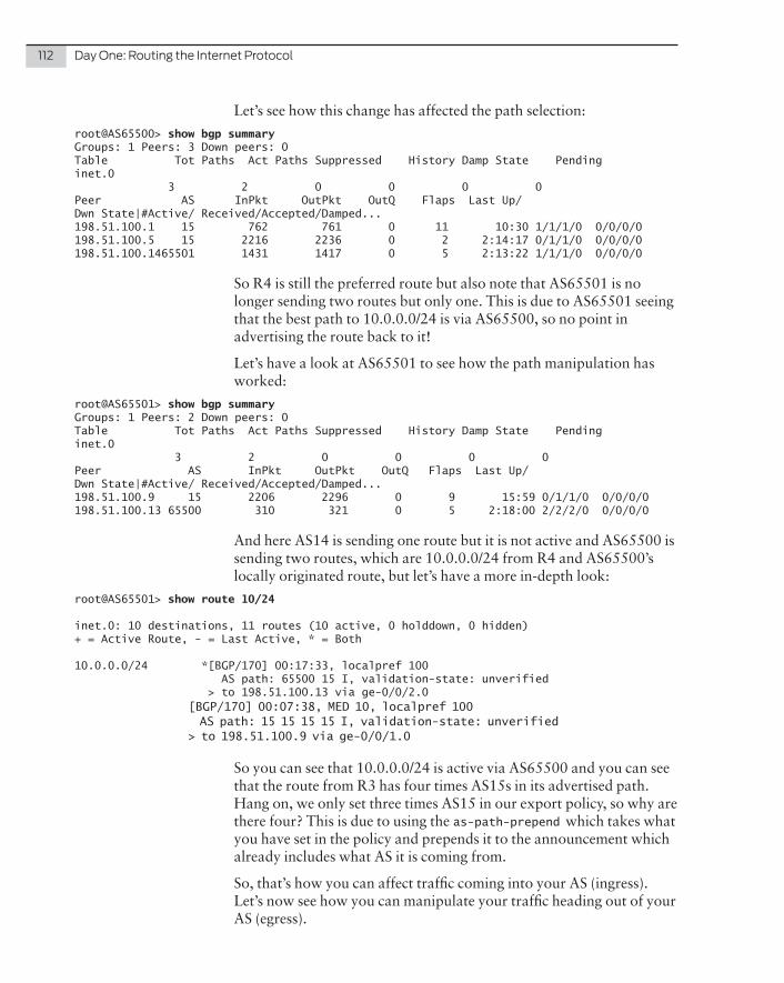
112 Day One: Routing the Internet Protocol
Let’s see how this change has affected the path selection:
root@AS65500> show bgp summary Groups: 1 Peers: 3 Down peers: 0Table Tot Paths Act Paths Suppressed History Damp State Pendinginet.0 3 2 0 0 0 0Peer AS InPkt OutPkt OutQ Flaps Last Up/Dwn State|#Active/ Received/Accepted/Damped...198.51.100.1 15 762 761 0 11 10:30 1/1/1/0 0/0/0/0198.51.100.5 15 2216 2236 0 2 2:14:17 0/1/1/0 0/0/0/0198.51.100.1465501 1431 1417 0 5 2:13:22 1/1/1/0 0/0/0/0
So R4 is still the preferred route but also note that AS65501 is no longer sending two routes but only one. This is due to AS65501 seeing that the best path to 10.0.0.0/24 is via AS65500, so no point in advertising the route back to it!
Let’s have a look at AS65501 to see how the path manipulation has worked:
root@AS65501> show bgp summary Groups: 1 Peers: 2 Down peers: 0Table Tot Paths Act Paths Suppressed History Damp State Pendinginet.0 3 2 0 0 0 0Peer AS InPkt OutPkt OutQ Flaps Last Up/Dwn State|#Active/ Received/Accepted/Damped...198.51.100.9 15 2206 2296 0 9 15:59 0/1/1/0 0/0/0/0198.51.100.13 65500 310 321 0 5 2:18:00 2/2/2/0 0/0/0/0
And here AS14 is sending one route but it is not active and AS65500 is sending two routes, which are 10.0.0.0/24 from R4 and AS65500’s locally originated route, but let’s have a more in-depth look:
root@AS65501> show route 10/24
inet.0: 10 destinations, 11 routes (10 active, 0 holddown, 0 hidden)+ = Active Route, - = Last Active, * = Both
10.0.0.0/24 *[BGP/170] 00:17:33, localpref 100 AS path: 65500 15 I, validation-state: unverified > to 198.51.100.13 via ge-0/0/2.0 [BGP/170] 00:07:38, MED 10, localpref 100 AS path: 15 15 15 15 I, validation-state: unverified > to 198.51.100.9 via ge-0/0/1.0
So you can see that 10.0.0.0/24 is active via AS65500 and you can see that the route from R3 has four times AS15s in its advertised path. Hang on, we only set three times AS15 in our export policy, so why are there four? This is due to using the as-path-prepend which takes what you have set in the policy and prepends it to the announcement which already includes what AS it is coming from.
So, that’s how you can affect traffic coming into your AS (ingress). Let’s now see how you can manipulate your traffic heading out of your AS (egress).

Chapter 7: Border Gateway Protcol (BGP) 113
AS65500 and AS65501 are now sending a default route, as well as their locally originated route, so one can reach the rest of the Internet. Why isn’t traffic sent destined to the Internet via AS65501?
Let’s have a look at 0.0.0.0/0 from the perspective of R3 and R4:root@R3> show route 0/0
inet.0: 21 destinations, 26 routes (21 active, 0 holddown, 0 hidden)+ = Active Route, - = Last Active, * = Both
0.0.0.0/0 *[BGP/170] 00:05:05, localpref 100 AS path: 65501 I, validation-state: unverified > to 198.51.100.10 via ge-0/0/3.0 [BGP/170] 00:02:31, localpref 100 AS path: 65500 I, validation-state: unverified > to 198.51.100.6 via ge-0/0/4.0 [BGP/170] 00:02:31, localpref 100, from 92.1.0.1 AS path: 65500 I, validation-state: unverified > to 10.0.0.6 via ge-0/0/2.0
Here, R3 is seeing a default route from AS65500, AS65501, and also via R4 (AS65500) using iBGP. Let’s have a look at R4 now:
root@R4> show route 0/0
inet.0: 20 destinations, 23 routes (20 active, 0 holddown, 0 hidden)+ = Active Route, - = Last Active, * = Both
0.0.0.0/0 *[BGP/170] 00:05:28, localpref 100 AS path: 65500 I, validation-state: unverified > to 198.51.100.2 via ge-0/0/3.0 [BGP/170] 00:08:01, localpref 100, from 93.1.0.1 AS path: 65501 I, validation-state: unverified > to 10.0.0.5 via ge-0/0/2.0
And R4 is seeing the default route from AS65500 and R3 (AS65501) via iBGP, and as you already know from the BGP best path selection process, eBGP is preferred over iBGP in any tie-breaker.
You might also notice that the paths have a local preference of 100 associated with them, even though they have set a local preference. This is due to the default local preference for BGP learned routes being set at 100. With local preference, the higher the value the more pre-ferred the route is, so let’s get back onto R3 and write an import policy to set the local preference to 200:
[edit protocols bgp group external neighbor 198.51.100.10]+ import SET-LOCALPREF-200;[edit policy-options]+ policy-statement SET-LOCALPREF-200 {+ then {+ local-preference 200;+ accept;+ }+ }
[edit]root@R3# commit

114 Day One: Routing the Internet Protocol
So after setting the local preference for routes learned via neighbor 198.51.100.10 (AS65501) to have a local preference of 200, let’s see how that has affected the routing table:
root@R3> show bgp summary Groups: 2 Peers: 5 Down peers: 1Table Tot Paths Act Paths Suppressed History Damp State Pendinginet.0 6 3 0 0 0 0Peer AS InPkt OutPkt OutQ Flaps Last Up/Dwn State|#Active/ Received/Accepted/Damped...90.1.0.1 15 306 321 0 8 1:54:17 0/0/0/0 0/0/0/091.1.0.1 15 749 749 0 1 11:46:41 Active92.1.0.1 15 182 178 0 4 1:16:33 0/0/0/0 0/0/0/0198.51.100.6 65500 385 384 0 2 2:51:51 0/3/3/0 0/0/0/0198.51.100.10 65501 115 111 0 9 48:54 3/3/3/0 0/0/0/0
Oops. It looks like the local preference for all routes learned from AS65501 was set, which includes AS65500’s locally originated route, which was not desired:
root@R3> show route protocol bgp
inet.0: 21 destinations, 24 routes (21 active, 0 holddown, 0 hidden)+ = Active Route, - = Last Active, * = Both
0.0.0.0/0 *[BGP/170] 00:20:07, localpref 200 AS path: 65501 I, validation-state: unverified > to 198.51.100.10 via ge-0/0/3.0 [BGP/170] 00:17:33, localpref 100 AS path: 65500 I, validation-state: unverified > to 198.51.100.6 via ge-0/0/4.0192.0.2.0/24 *[BGP/170] 00:51:47, localpref 200 AS path: 65501 I, validation-state: unverified > to 198.51.100.10 via ge-0/0/3.0 [BGP/170] 02:53:48, localpref 100 AS path: 65500 65501 I, validation-state: unverified > to 198.51.100.6 via ge-0/0/4.0203.0.113.0/24 *[BGP/170] 00:51:47, localpref 200 AS path: 65501 65500 I, validation-state: unverified > to 198.51.100.10 via ge-0/0/3.0 [BGP/170] 02:54:44, localpref 100 AS path: 65500 I, validation-state: unverified > to 198.51.100.6 via ge-0/0/4.0
Let’s use the power of the Junos OS routing policy to fix this and only set the local preference for 0/0 learned from AS65501:
root@R3# show | compare [edit policy-options policy-statement SET-LOCALPREF-200]+ from {+ route-filter 0.0.0.0/0 exact;+ }
[edit]root@R3# commit
With the addition of the patch, the policy is now very specific. It looks like this:

Chapter 7: Border Gateway Protcol (BGP) 115
root@R3# show policy-options policy-statement SET-LOCALPREF-200 from { route-filter 0.0.0.0/0 exact;}then { local-preference 200; accept;}
This policy now says that if the route is exactly 0.0.0.0/0 then it will set the local preference to 200. As BGP policy has an implicit accept, any routes that do not match 0.0.0.0/0 will still be accepted but with the default local pref of 100. Let’s see how this looks now:
root@R3> show route protocol bgp
inet.0: 21 destinations, 25 routes (21 active, 0 holddown, 0 hidden)+ = Active Route, - = Last Active, * = Both
0.0.0.0/0 *[BGP/170] 00:30:04, localpref 200 AS path: 65501 I, validation-state: unverified > to 198.51.100.10 via ge-0/0/3.0 [BGP/170] 00:27:30, localpref 100 AS path: 65500 I, validation-state: unverified > to 198.51.100.6 via ge-0/0/4.0192.0.2.0/24 *[BGP/170] 01:01:44, localpref 100 AS path: 65501 I, validation-state: unverified > to 198.51.100.10 via ge-0/0/3.0 [BGP/170] 03:03:45, localpref 100 AS path: 65500 65501 I, validation-state: unverified > to 198.51.100.6 via ge-0/0/4.0203.0.113.0/24 *[BGP/170] 03:04:41, localpref 100 AS path: 65500 I, validation-state: unverified > to 198.51.100.6 via ge-0/0/4.0 [BGP/170] 00:08:14, localpref 100, from 92.1.0.1 AS path: 65500 I, validation-state: unverified > to 10.0.0.6 via ge-0/0/2.0 [BGP/170] 01:01:44, localpref 100 AS path: 65501 65500 I, validation-state: unverified > to 198.51.100.10 via ge-0/0/3.0
Fantastic. The network is preferring 0.0.0.0/0 from AS65501 and all other routes are at their default.
R4 also shows that it is preferring the path for 0.0.0.0/0 from AS65501, going via R3 who has advertised it via iBGP:
root@R4> show route protocol bgp
inet.0: 20 destinations, 23 routes (20 active, 0 holddown, 0 hidden)+ = Active Route, - = Last Active, * = Both
0.0.0.0/0 *[BGP/170] 00:18:12, localpref 200, from 93.1.0.1 AS path: 65501 I, validation-state: unverified > to 10.0.0.5 via ge-0/0/2.0 [BGP/170] 00:30:51, localpref 100 AS path: 65500 I, validation-state: unverified > to 198.51.100.2 via ge-0/0/3.0

116 Day One: Routing the Internet Protocol
So, traffic has been affected. Note how it exits AS15 using the local preference and is manipulated into how it enters the AS. Looking at the small amount of configuration taken to achieve this, you can see how powerful the Junos OS route policy can be, especially when tied into BGP.
Summary
You have made it to the end of the BGP chapter and the rather in-depth tutorial!
No matter how much BGP is explained, explanations only seem to scratch the surface of this powerful protocol. In this tutorial you have learned the differences between iBGP and eBGP, best path computa-tion, and how you can manipulate how the outside world views your prefixes. Through the use of some simple routing policy you have also been able to control how traffic exits the AS.
The Junos OS with its very granular routing policy allows the user to leverage the true power and scale of BGP with what can be considered some very simple CLI commands. It’s no surprise that due to BGP’s maturity as a protocol and it’s scalability that it has also been used for the likes of VPLS, L2VPN, and EVPN, which allows it to carry MAC address information within its BGP updates.
Some great information on BGP can be found at the following links on Wikipedia and at the Juniper’s TechLibrary:
https://en.wikipedia.org/wiki/Border_Gateway_Protocol
http://www.juniper.net/techpubs/en_US/junos15.1/information-prod-ucts/pathway-pages/config-guide-routing/config-guide-routing-bgp.html
Also recommended are the following books:
http://www.juniper.net/us/en/training/jnbooks/oreilly-juniper-library/junos-enterprise-routing/
http://www.ciscopress.com/store/routing-tcp-ip-volume-ii-ccie-profes-sional-development-9781578700899

If, for a moment, we were to compare routers to PCs in terms of memory usage, PCs have an advantage in that more memory can usually be quite easily purchased and installed.
Routers, on the other hand, do not have virtual memory. Memory can be expanded, but it’s usually at a premium and even then, on a live network, the administrator needs to find downtime to install it. Memory management on a router is very critical and potential issues should be identified and corrected before they become serious.
The purpose of routers is to route data between subnets. The router needs to know which subnets to have reachability to because if the router receives a packet with a destination the router is not aware of, the router will drop the packet.
And every route the router is aware of needs to be stored in the routing table, so the more routes that are in the routing table the more memory is consumed. To put this into perspective for a moment, if the entire BGP table from the Internet was loaded into a router, the BGP data-base would consume over 1.7GB of memory. If a router on a corporate LAN has 1GB RAM, the router simply would not have enough memory.
Chapter 8
Route Summarization

118 Day One: Routing the Internet Protocol
In the case of Internet routes being redistributed into a corporate network, under normal circumstances, the default route of 0.0.0.0/0 is advertised into the LAN so that routers do not need to know every subnet that is available on the Internet, a router just needs to know that if a particular subnet is not in its routing table, then it should send the packet to the default route.
Corporate networks, on the other hand, are different, and often have hundreds or thousands of subnets where each router needs to know how to reach each individual subnet. This means the memory on each router is now being filled with those routes.
Summarization is a means of compressing the routing table and by using summarization, multiple networks can be joined so they appear in the routing table as a single subnet instead of as multiple entries.
Figure 8.1 shows an example of multiple subnets being summarized. In this case there are six routers. Routers A through E are each attached to a network that begins 10.10.x.x. The link between routers E and F uses subnet 172.23.7.0/24.
Figure 8.1 Summarizing Four Subnets into a Single Route
In this situation, router F could have a default route to router E, however that would mean that all traffic is sent to router E, whether router E has the route in its routing table or not. If summarization were to be used, then instead of creating a default route, the 10.10.x.x networks could be made into the single network 10.10.0.0/21.
With summarization, the administrator would use simple bit matching to determine which common bits are in use with each subnet. The bit matching should be as long as possible, which in Figure 9.1 is 21 bits. When router F receives a packet destined for one of the subnets that

Chapter 8: Route Summarization 119
10.10.0.0/21 covers, it will immediately forward it to router E. Should the subnet not be covered by that route, for example 10.10.100.0/24, then router F will discard the packet.
Although Figure 8.1 is a small LAN and therefore would not benefit from summarization, a multi-national corporation with offices in the U.S., Europe, and the Middle East might. In this situation, the offices in the U.S. could use subnets beginning with 10.100.x.x, whereas Europe could use 10.150.x.x, and the Middle East could use networks beginning 10.200.x.x.
The routers that connect, say, the U.S. to the WAN could then summarize the routes to 10.100.0.0/x. This way the routers in Europe and the Middle East will receive a single route instead of potentially hundreds of routes. The amount of subnets could increase substantially if each subnet was a /25 or less.
Configuring Route Summarization
In the following scenario, the ASBRs, which are routers vMX2 and vMX4, will be configured to take three subnets that are advertised by IS-IS and summarize them into a single subnet. Before this can be done, it is important to realize that if a subnet is directly connected to a router – for example subnets 10.10.1.0/24 and 10.10.2.0/24 are directly con-nected to router vMX2 – then these subnets will not be summarized and will still be advertised as separate subnets by OSPF.
In order to work around this limitation, three new IP addresses have been added to the loopback interface of router vMX6. These have therefore created three new subnets and as IS-IS has already been configured to advertise subnets connected to interface lo0.0, so these should automati-cally start appearing in the routing table of all routers in the LAN:
root@VMX6> show interfaces terse lo0.0Interface Admin Link Proto Local Remotelo0.0 up up inet 10.20.1.1/24 10.20.2.1/24 10.20.3.1/24 192.168.1.4 --> 0/0 iso 49.0003.0001.0001.0004
Figure 8.2 gives a graphical representation of what this scenario achieves. The three subnets from router vMX6 are summarized to a single route, 10.20.0.0/22. At the same time, the three subnets from router vMX6 are then filtered to prevent these separate subnets from being advertised to routers vMX0 and vMX1 in the OSPF domain.

120 Day One: Routing the Internet Protocol
Figure 8.2 Summarizing Routes from Router vMX6
For the purposes of this scenario, router vMX1 will be used to test whether the summarization has worked successfully and to test reach-ability, and if the show route 10.20.0.0/16 command were to be run on this router, the subnets should be listed twice, once as a /24 and once as a /32, as these subnets were added to the loopback interface and as such OSPF treats these as host routes. Let’s check:
root@VMX1> show route 10.20.0.0/16
inet.0: 29 destinations, 32 routes (29 active, 0 holddown, 0 hidden)+ = Active Route, - = Last Active, * = Both
10.20.1.0/24 *[OSPF/150] 00:00:31, metric 2, tag 0 > to 10.5.0.2 via ge-0/0/2.010.20.1.1/32 *[OSPF/150] 00:00:31, metric 2, tag 0 > to 10.5.0.2 via ge-0/0/2.010.20.2.0/24 *[OSPF/150] 00:00:31, metric 2, tag 0 > to 10.5.0.2 via ge-0/0/2.010.20.2.1/32 *[OSPF/150] 00:00:31, metric 2, tag 0 > to 10.5.0.2 via ge-0/0/2.010.20.3.0/24 *[OSPF/150] 00:00:31, metric 2, tag 0

Chapter 8: Route Summarization 121
> to 10.5.0.2 via ge-0/0/2.010.20.3.1/32 *[OSPF/150] 00:00:31, metric 2, tag 0 > to 10.5.0.2 via ge-0/0/2.0
Router vMX1 should also be able to ping one of the IP addresses too, in this case 10.20.1.1:
root@VMX1> ping 10.20.1.1PING 10.20.1.1 (10.20.1.1): 56 data bytes64 bytes from 10.20.1.1: icmp_seq=0 ttl=63 time=4.105 ms64 bytes from 10.20.1.1: icmp_seq=1 ttl=63 time=3.881 ms64 bytes from 10.20.1.1: icmp_seq=2 ttl=63 time=5.666 ms64 bytes from 10.20.1.1: icmp_seq=3 ttl=63 time=4.346 ms^C--- 10.20.1.1 ping statistics ---4 packets transmitted, 4 packets received, 0% packet lossround-trip min/avg/max/stddev = 3.881/4.500/5.666/0.693 ms
In order to perform summarization, two things need to be added to the configuration. The first is what is known as an aggregate route. This tells the Junos OS what the routes will be summarized to. In this case, the IP addresses added on router vMX6 can be summarized to a single route – 10.20.0.0/22:
set routing-options aggregate route 10.20.0.0/22
While it is possible to summarize these routes to 10.20.0.0/16, it’s considered best practice to use the longest match possible so that the router isn’t processing unnecessary traffic. For example, if someone attempted to send a packet to 10.20.5.1, by using a /22 prefix, the pack-et would be dropped by the router, whereas with a /16 prefix, the router would need to process the packet and forward it to the ASBR. This would affect each router in the path of the packet all for the ASBR to discard the packet anyway.
Once the aggregate router has been created, the routing protocol needs to be told to export this route to neighbors. This is done by using the same policy statement that was created when performing redistribu-tion. As with redistribution, the policy statement works from the top down and stops once there is a match, therefore the term to tell OSPF to redistribute the aggregate route should ideally be added first.
In this scenario, the changes will first be made on router vMX4. The policy statement in use on vMX4 currently is:
[edit]root@VMX4# show policy-options policy-statement RIP-TO-OSPFterm 1 { from { protocol rip; prefix-list ONESEVENTWOTWENTYTHREEONE; } then reject;}

122 Day One: Routing the Internet Protocol
term 2 { from protocol rip;}then accept;
As the policy statement is using numbered terms, it would be ideal to change Term 2 to Term 3, and the term currently numbered 1 to Term 2. The new term will then be added as Term 1, just to keep things tidy:
rename policy-options policy-statement RIP-TO-OSPF term 2 to term 3rename policy-options policy-statement RIP-TO-OSPF term 1 to term 2
After a quick check to see if the terms have been renumbered correctly, Term 1 can then be recreated with a new rule:
[edit]root@VMX4# show policy-options policy-statement RIP-TO-OSPFterm 2 { from { protocol rip; prefix-list ONESEVENTWOTWENTYTHREEONE; } then reject;}term 3 { from protocol rip;}then accept;
The new term is really just redistributing from the protocol aggregate to OSPF, therefore the term needs to specify to match routes from protocol aggregate and to match the subnet specified when added the routing option, which in this case is 10.20.0.0/22. Finally, an accept has been added at the end of this term, although in theory, the accept at the end of the policy statement should already accept this term:
set policy-options policy-statement RIP-TO-OSPF term 1 from protocol aggregateset policy-options policy-statement RIP-TO-OSPF term 1 from route-filter 10.20.0.0/22 exactset policy-options policy-statement RIP-TO-OSPF term 1 then accept
Once this is added, if the policy statement is viewed, it’s interesting to see that the new term has been added after Term 3. When a policy statement is numbered, the Junos OS only sees this as a label as opposed to a numerical value, so in reality this term could have been called summarize, but in the case of this scenario, the numbering convention was retained:
root@VMX4# show policy-options policy-statement RIP-TO-OSPFterm 2 { from { protocol rip; prefix-list ONESEVENTWOTWENTYTHREEONE; } then reject;}

Chapter 8: Route Summarization 123
term 3 { from protocol rip;}term 1 { from { protocol aggregate; route-filter 10.20.0.0/22 exact; } then accept;}then accept;
In order to move Term 1 up the list, the insert command is used. In order to move Term 1 to before Term 2, the following command is applied:
insert policy-options policy-statement RIP-TO-OSPF term 1 before term 2
The policy statement should now appear in the correct order:
[edit]root@VMX4# show policy-options policy-statement RIP-TO-OSPFterm 1 { from { protocol aggregate; route-filter 10.20.0.0/22 exact; } then accept;}term 2 { from { protocol rip; prefix-list ONESEVENTWOTWENTYTHREEONE; } then reject;}term 3 { from protocol rip;}then accept;
Router vMX4 has now been configured, but as there are two ASBRs, the summarization won’t be effective in decreasing the size of the routing table, therefore the same configuration should be applied to vMX2. The command to add the aggregate route should be the same on both ASBRs:
set routing-options aggregate route 10.20.0.0/22
The policy statement on router vMX2 is called IS-IS-TO-OSPF as opposed to RIP-TO-OSPF on vMX4. The first step is to rename the terms to match those changes made on vMX4. Although in theory the terms could be given different names, it is better to keep naming conventions common across your network, as it helps when it comes to supporting it later on:

124 Day One: Routing the Internet Protocol
rename policy-options policy-statement ISIS-TO-OSPF term 2 to term 3rename policy-options policy-statement ISIS-TO-OSPF term 1 to term 2
Once the terms have been renamed, the new term is created:
set policy-options policy-statement ISIS-TO-OSPF term 1 from protocol aggregateset policy-options policy-statement ISIS-TO-OSPF term 1 from route-filter 10.20.0.0/22 exactset policy-options policy-statement ISIS-TO-OSPF term 1 then accept
Finally, the new term is inserted before what is now term 2:
insert policy-options policy-statement ISIS-TO-OSPF insert term 1 before term 2
Once the configuration has been committed, the routing table on vMX1 can be checked to confirm the new aggregate route has been added (bold in the output). What is also unexpected is that the routes, even though they have been summarized, are still appearing in the routing table. Instead of decreasing the size of the routing table, it has instead increased it:
root@VMX1> show route 10.20.0.0/16
inet.0: 31 destinations, 34 routes (31 active, 0 holddown, 0 hidden)+ = Active Route, - = Last Active, * = Both
10.20.0.0/22 *[OSPF/150] 00:04:38, metric 0, tag 0 > to 10.3.0.1 via ge-0/0/1.010.20.1.0/24 *[OSPF/150] 00:08:51, metric 2, tag 0 > to 10.5.0.2 via ge-0/0/2.010.20.1.1/32 *[OSPF/150] 00:08:51, metric 2, tag 0 > to 10.5.0.2 via ge-0/0/2.010.20.2.0/24 *[OSPF/150] 00:08:51, metric 2, tag 0 > to 10.5.0.2 via ge-0/0/2.010.20.2.1/32 *[OSPF/150] 00:08:51, metric 2, tag 0 > to 10.5.0.2 via ge-0/0/2.010.20.3.0/24 *[OSPF/150] 00:08:51, metric 2, tag 0 > to 10.5.0.2 via ge-0/0/2.010.20.3.1/32 *[OSPF/150] 00:08:51, metric 2, tag 0 > to 10.5.0.2 via ge-0/0/2.0
To prevent these subnets from being advertised, a filter should be applied to the ASBRs. In this case, the filter is first applied to router vMX2. The issue is that there are now three terms that need renaming, therefore, instead of renaming them, the term will simply be called 0.5:
set policy-options policy-statement ISIS-TO-OSPF term 0.5 from protocol isis
As you may recall, in Chapter 6 the term to filter the router included a prefix-list. The configuration in this scenario uses a different method of specifying which routes to suppress – a route-filter. By using a route filter, there is no need to create a prefix list before creating the policy statement, in addition the exact, orlonger, and longer key-words can be used to determine whether to match just that subnet, or subnets that begin the same, or ones that don’t begin the same but match the rest of the subnet.

Chapter 8: Route Summarization 125
NOTE The best resource to learn more about route filters is from Juniper’s Tech Library. You can read more about route filters at the following URL: http://www.juniper.net/techpubs/en_US/junos15.1/topics/usage-guidelines/policy-configuring-route-lists-for-use-in-routing-policy-match-conditions.html.
In this scenario, you don’t want to suppress 10.20.0.0/22 but you do want to suppress routes that are longer than this: 10.20.1.0/24, 10.20.2.0/24, and 10.20.3.0/24, therefore the route-filter command is followed with the keyword longer:
set policy-options policy-statement ISIS-TO-OSPF term 0.5 from route-filter 10.20.0.0/22 longerset policy-options policy-statement ISIS-TO-OSPF term 0.5 then reject
Here, Term 0.5 is inserted before Term 1:
insert policy-options policy-statement ISIS-TO-OSPF insert term 0.5 before term 1
Once done, the same rules can be applied to router vMX4 and the term inserted before term 1:
set policy-options policy-statement RIP-TO-OSPF term 0.5 from protocol ripset policy-options policy-statement RIP-TO-OSPF term 0.5 from route-filter 10.20.0.0/22 longerset policy-options policy-statement RIP-TO-OSPF term 0.5 then reject
insert policy-options policy-statement RIP-TO-OSPF term 0.5 before term 1
After committing these changes, router vMX1’s routing table should be checked once more to ensure that the route 10.20.0.0/22 is present, but the individual /24 routes are not:
root@VMX1> show route 10.20.0.0/16
inet.0: 25 destinations, 28 routes (25 active, 0 holddown, 0 hidden)+ = Active Route, - = Last Active, * = Both
10.20.0.0/22 *[OSPF/150] 00:05:57, metric 0, tag 0 > to 10.3.0.1 via ge-0/0/1.0
Finally, a ping to one of the subnets should prove that routes from vMX1 to vMX6 have not been suppressed inadvertently:
root@VMX1> ping 10.20.1.1PING 10.20.1.1 (10.20.1.1): 56 data bytes64 bytes from 10.20.1.1: icmp_seq=0 ttl=63 time=5.421 ms64 bytes from 10.20.1.1: icmp_seq=1 ttl=63 time=6.610 ms64 bytes from 10.20.1.1: icmp_seq=2 ttl=63 time=4.341 ms64 bytes from 10.20.1.1: icmp_seq=3 ttl=63 time=6.751 ms^C--- 10.20.1.1 ping statistics ---4 packets transmitted, 4 packets received, 0% packet lossround-trip min/avg/max/stddev = 4.341/5.781/6.751/0.979 ms

126 Day One: Routing the Internet Protocol
Summary
Summarization is useful for several reasons. It can decrease the number of routes in a routing table, and this in turn increases available memory and reduces the amount of processing the router needs to perform.
If you use the topology given at the beginning of this book, there are 11 subnets. Summarization could in theory decrease this number to just three. That said, it’s unlikely because in this case the MX routers that are in this LAN wouldn’t really benefit from this approach, therefore summarization really needs to be used when subnets are in their hundreds for the benefit to be felt.
Summarization could be used when there are two large sites that are connected via a WAN connection. The administrator could use 172.x.x.x addresses on one site and 10.x.x.x addresses on the other site and summarize the addresses on both sites to a single address.
Where to Go Next
While the authors have attempted to make this book as informative as possible, it is nonetheless a “fundamentals” book, meaning there’s enough information to get you started, but that doesn’t mean you can stop here.
MORE? If you want to learn more about the protocols covered in this book, visit the Day One library and browse the Junos OS Fundamentals Series suite of books: http://www.juniper.net/dayone. There are also complete documentation guides, solutions, and network configuration examples for the entire Junos OS at Juniper’s TechLibrary: http://www.juniper.net/documentation.