day to day variation of ionosphere electron and ion ...€¦ · seasonal and solar activity...
TRANSCRIPT

Al-Ubaidi and Gmayhs Iraqi Journal of Science, 2015, Vol 56, No.4A, pp: 2996-3014
____________________________
*Email: [email protected] 2996
Day to Day variation of Ionosphere Electron and Ion Temperature during
Great and Severe Geomagnetic Storms
Najat M. R. Al-Ubaidi*, Karam H. Gmayhs
Department of Astronomy & Space, College of Science, Baghdad University, Baghdad, Iraq
Abstract
The ionospheric characteristics exhibit significant variations with the solar cycle,
geomagnetic conditions, seasons, latitudes and even local time. Representation of
this research focused on global distribution of electron (Te) and ion temperatures
(Ti) during great and severe geomagnetic storms (GMS), their daily and seasonally
variation for years (2001-2013), variations of electron and ion temperature during
GMS with plasma velocity and geographic latitudes. Finally comparison between
observed and predicted Te and Ti get from IRI model during the two kinds of storm selected. Data from satellite Defense Meteorological Satellite Program (DMSP) 850
km altitude are taken for Te, Ti and plasma velocity for different latitudes during
great and severe geomagnetic storms from years 2001 to 2013 according to what is
available appeared that there is 22 events for severe and great geomagnetic storms
happened during years 2001-2005 only from years selected, from maximum solar
cycle 23. From data analysis, in general the temperature of the electron is greater
than the temperature of the ion, but there are some disturbances happened during the
storm time, in the day there is fluctuation in values of Te and Ti with the value of Ti
greater than Te. Through the Dst index, Te and Ti do not depend on the strength of
the geomagnetic storm. Plasma velocity variation shows the same profile of Te and
Ti variation during the storm time and there is a linear relation between (Te) & (Ti) and plasma velocity. The variation of electron and ion temperature with geographic
latitude during severe and great storms appears that as the latitude increases the
temperature of ions increases reaches its maximum value approximately 80000K at
poles.
From comparing the predicted Te and Ti values calculating from IRI model
during the great and severe storms with observed values, it’s found that the predicted
values from IRI model much less than the observed values and the variation was
nonlinear along 24 hours, from this we can conclude that the model must be
corrected for Te and Ti for these two kinds of storms.
Keywords: Electron and Ion Temperature, Geomagnetic Storm, IRI model.
التغيرات من يوم الخر في درجات حرارة االلكترونات وااليونات لاليونوسفير أثناء العواصف الجيومغناطيسية الشديدة والقوية
غميس , كرم حنون*نجاة محمد رشيد رؤوف العبيدي ، بغداد، العراق، كلية العلوم، جامعة بغدادقسم الفلك والفضاء
خالصةالتالفات كبيرة مع الدورة الشمسية، وطبيعة المجال المغناطيسي لالرض خصائص الغالف األيوني يبدي اخ
والمواسم وخطوط العرض وكذلك التوقيت المحلي. يهدف البحث الى دراسة توزيع درجات حرارة االلكترونات -1002وااليونات وتغيراتها اليومية والفصلية خالل العواصف الجيومغناطيسية الشديدة والكبيرة ولالعوام
ISSN: 0067-2904 GIF: 0.851

Al-Ubaidi and Gmayhs Iraqi Journal of Science, 2015, Vol 56, No.4A, pp: 2996-3014
2997
وكذلك دراسة درجات حرارة االلكترونات وااليونات مع سرعة البالزما وخطوط العرض الجغرافية اثناء 1023نوعي العواصف المختارة في هذه الدراسة. واخيرا جرت مقارنة بين قيم درجات حرارة االلكترونات وااليونات
ثناء العاصفتين المختارة. البيانات أخذت أ IRI ها والمحسوبة من الموديل العالميالمرصودة مع القيم المتنبأ بكم لدرجات حرارة االلكترونات وااليونات وكذلك سرعة 050وعلى ارتفاع DMSPمن القمر الصناعي
البالزمة ولخطوط عرض مختلفة ولنوعي العواصف الجيومغناطيسية التي تم اختيارها لهذه الدراسة من االعوام عاصفة جيومغناطيسية شديدة وقوية حدثت خالل 11تبين ان هنالك ولما هو متوفر ، 1023ولغاية 1002
فقط من السنوات التي اختيرت للدراسة وهي من ضمن الدورة الشمسية العالية. من 1005-1002االعوام خالل تحليل البيانات وجد وبصورة عامة أن درجات حرارة االلكترونات أعلى من درجات حرارة االيونات ولكن
ة العواصفحدثت اضطرابات وتذبذبات في قيم درجات الحرارة بحيث اصبحت خالل النهار درجات اثناء فتر تبين ان Dstحرارة االيونات اعلى من درجات حرارة االلكترونات. من خالل عامل االضطراب المغناطيسي
يسية. سرعة البالزما قيم درجات حرارة االلكترونات وااليونات التعتمد على شدة او نوع العاصفة الجيومغناطتظهر تغيرات تكاد تكون مشابهة لتغيرات درجات حرارة االلكترونات وااليونات اثناء نوعي العاصفتين المختارة وان هنالك تقريبا عالقة خطية بينهم. التغيرات في درجات الحرارة مع خطوط العرض أثناء العواصف بينت بأن
العرض وصوال لمنطقة االقطاب بحيث تصل في بعض االحيان قيم درجات الحرارة تزداد مع زيادة خطوطكلفن. أجريت مقارنة بين قيم درجات الحرارة المرصودة لاللكترونات وااليونات مع القيم 00000اعلى قيم لها
وجد بأن القيم المحسوبة اقل من المرصودة وهنالك تغيرات بين IRIالمتنبأ بها والمحسوبة من الموديل النظري يمتين لالربع وعشرين ساعة من يوم العاصفة المختارة ان هذه التغيرات غير خطية وعليه يجب اجراء الق
تصحيح للموديل النظري لنوعي العواصف الشديدة والقوية.
Introduction:
The ionosphere is the ionized portion of the upper atmosphere of the Earth. The photoionization of neutral molecules is the main source of plasma in the ionosphere. Then several processes may occur,
chemical reactions between the ions produced and the neutrals take place, ions recombine with the
electrons, ions diffuse to either higher or lower altitudes, or they are transported via neutral wind effects. Notice that the Earth’s intrinsic magnetic field, which is dipolar at ionospheric altitudes,
strongly influences the diffusion and transport effects. At different latitudes, different physical
processes dominate, but the electron density variation with altitude which leads to variation in temperature still displays the same basic structure except that at high latitudes the O
+ density differs
from that at mid-latitudes [1].
Within the lowest regions of the ionosphere, electrons and ions typically possess equal
temperatures and move at a characteristic thermal speed which is dictated by both this temperature and the mass of the charged particle. With an increasing altitude however, the difference between the
temperatures increases and at the F region peak, typical electron and ion temperatures are 2000K and
1400K respectively. Any external driving force, such as that supplied by an electric field, will also serve to accelerate the charged particles and consequently act as a source of energy that heats the
plasma. As a result of the large difference in mass between the ions and electrons, it is principally the
electron temperature that is enhanced significantly when the plasma is heated [2]. The high-latitude ionosphere is strongly coupled to the magnetosphere–thermosphere system via electric fields, particle
precipitation, field-aligned currents, heat flows, frictional interac- tions, chemical interactions, and
feedback mechanisms, and these have a significant impact on the high-latitude ionospheric density and
thermal structure [3]. In an effort to understand the effects that these processes have on the iono- sphere, many numerical physics-based models have been developed over the years and these models
have been very useful in understanding ionospheric behavior [4].
Previous Studies: Several studies are made conducted in this regard mention some of them related to our study,
Buonsato M. J. (1989) studied the Millstone Hill incoherent scatter (IS) observations of electron
density (Ne), electron temperature (Te) and ion temperature (Ti) which are compared with the
International Reference Ionosphere (IRI-86) model for both noon and midnight, for summer, equinox and winter, at both solar maximum and minimum. Generally it shown that in winter Ne larger than in

Al-Ubaidi and Gmayhs Iraqi Journal of Science, 2015, Vol 56, No.4A, pp: 2996-3014
2998
summer, this is apparently due to photoelectron heating during winter [5]. Forme F. et al. (1993)
Performed one-dimensional time-dependent model calculations of the effects of low frequency
turbulence, due to three different current driven instabilities, on the ion and electron temperatures in
the topside ionosphere [6]. Pavlov A. V. et al. (2001) studied a comparison of the electron density and temperature behavior measured in the ionosphere during the period 25–29 June 1990. The evaluation
values of the nighttime additional heating rate that should be added to the normal photoelectron
heating in the electron energy equation in the plasmasphere region above 5000 km along the magnetic field line to explain the high electron temperature [7]. Sethi N. K. et al. (2004). Studied Incoherent
scatter radar data from Arecibo, for solar maximum and minimum periods, are used to study the
seasonal and solar activity variations in (Te) for noontime conditions. In spite of large day-to-day variations, clear seasonal variations in average Te can be identified for both solar activity periods, with
winter temperatures significantly higher in the topside (400–700 km) ionosphere [8]. Gulyaeva T. L.
and J.E. Titheridge (2006). Analyzed a plasmasphere extension has been incorporated in the IRI using
the Russian standard model of the ionosphere SMI, at altitudes from 1000 km to the plasmapause (636,000 km). [9]. Jiuhou Lei et al., (2007) studied ionospheric (Te) data for more than two solar
cycles are compared with the theoretical Te calculated from the Model (NCAR-TIEGCM) to
investigate the temporal variations of Te. The simulations show that the daytime bulge of Te tends to occur at low latitudes and high solar activity, as seen in the observations, and the significant morning
peak at low solar activity over Arecibo is associated with the equatorial anomaly [10].
M.V. Klimenko, et al .,(2008). Worked on The results from the numerical calculations of the global distribution of topside ionospheric parameters such as H+ ions and ion and electron temperatures up to
1500km height are presented for equinoctial conditions at solar minimum [11]. Schunk A. and Nagy
(2010) found the theory and an observation relating to electron temperatures in the F region, the
review covers electron temperature variations with altitude, latitude, local time, season, geomagnetic activity, and solar cycle [12]. David M. et al., (2011) studied the electron energy balance in the
ionosphere is affected by numerous local heating include thermal conduction and thermoelectric heat
flow [4]. In (1913) Slominska and Hanna studied is oriented on the dataset gathered in 2005and 2008. Within conducted analysis, global maps of electron temperature for months of equinoxes and solstices
have been developed. Furthermore, simultaneous studies on two-dimensional time series based on
DEMETER measurements and predictions obtained with the IRI-2012 model supply examination of
the topside ionosphere during recent deep solar minimum [13]. De Meneses F.C. et al., (2013) studied the simultaneous in-situ measurements of Ne and Te in the nighttime equatorial region were
performed by a rock experiment launched under solar minimum and geomagnetic quiet conditions
[14]. The purpose of this paper is to study the diurnal variation of ionospheric electron and ion temperature during severe and great geomagnetic storms, then to reveal the validity of IRI model
during these kinds of storms.
Temperature of Ionosphere: Temperature can be defined in different ways due to different degrees of freedom – Otherwise the
definition of temperature is the same for all matter (i.e. fluids, solid matter, gas and plasma):
temperature is the energy related to random motion. There are several kinds of random motion:
translational, rotational and vibrational each one contributes with different degrees of freedom to the determination of the temperature in thermal equilibrium. Each degree (G) of freedom contributes with
(G kT)/2 to the total energy, where T is the temperature, (k) is Boltzmann’s constant and G is typically
3 in plasma physics applications (F-region and topside the region above F2 layer [8]). In the ionosphere, the temperature (thermal energy) of a particle is directly proportional to average random
kinetic (translational) energy and the neutral temperature will in general increase dramatically above
the mesopause (~80 km) into the thermosphere, until it reaches an overall maximum of about 1000 K. However, the maximum and minimum of the neutral temperature depend on time, latitude, solar
activity. Typically, between midnight and noon during solar minimum (maximum), the temperature
varies between approximately (1000 – 1700 K)[15]. The neutral temperature maximum will typically
occur at about 400 km, in the region called exobase, and then the temperature becomes constant with altitude in the exosphere. In the exosphere (> 600 km), individual atoms have the possibility to escape
from the Earth’s gravitational attraction if the temperature is high enough (escape velocity ve
=(2GM/r)0.5
where G is a gravitational constant, M the mass of the planet, (r) the distance between planet center and position).The background exospheric temperature is normally between 1000 and

Al-Ubaidi and Gmayhs Iraqi Journal of Science, 2015, Vol 56, No.4A, pp: 2996-3014
2999
1500 K, too low to escape, but if the temperature increases, so will the velocity, and the minimum
escape velocity is about 9.7 km/s at 2000 km. This is somewhat less than the escape velocity
(½mv2=3/2KT) at the Earth’s surface, which is ~11.2 km/s. In general, it requires a huge temperature
for O and He to escape. A factor 16 and 4 more than for H is related to O and He, respectively, and the escape temperature is equal to or greater than 4900 K (> 0.63 eV) at about 500 km. Thus the escape
velocity (~11 km/s) is more than twice the mean thermal velocity (4.98 km/s) of atomic hydrogen at a
temperature of 1000 K [16] as shown in Figure-1.
Figure 1- Typical profiles of neutral temperature [17].
Geomagnetic Storm index Disturbance storm time (Dst): The Dst index defines the effectiveness of geomagnetic storm. The negative value of Dst index
indicates the commencement of the storm. The intensity of storm depends on the value of Dst index.
As the Dst index becomes more and more negative the storm also becomes stronger and stronger. Dst
is expressed in nanoteslas (nT) and is based on the average value of the horizontal component of the Earth's magnetic field measured hourly at four near-equatorial geomagnetic observatories [18].
The minimum Dst value reached is often used to classify the strength of a geomagnetic storms as in
table-1.
Table 1- Geomagnetic storm classification [18].
Dst value Storm type
Minimum Dst below -20 nT Weak storm
Minimum Dst below -50 nT Moderate storm
Minimum Dst below -100 nT Strong storm
Minimum Dst below -200 nT Severe storm
Minimum Dst below -320 nT Great storm
International Reference Ionosphere Model (IRI):
The International Reference Ionosphere (IRI) project was initiated by the Committee on Space
Research(COSPAR) and by the International Union of Radio Science (URSI) in the late sixties with
the goal of establish in international standard for the specification of ionospheric parameters based on all worldwide available data from ground-based as well as satellite observations. COSPAR and URSI
specifically asked for an empirical model to avoid the uncertainties of the evolving theoretical
understanding of ionospheric processes and coupling to the regimes below and above [48]. From early on the model was made available in electronic form as a FORTRAN program and more recently also
as an interactive web interface accessible from the IRI homepage. IRI describes monthly average of

Al-Ubaidi and Gmayhs Iraqi Journal of Science, 2015, Vol 56, No.4A, pp: 2996-3014
3000
the electron density, electron and ion temperature, ion composition (O+, H+, N+,He+, O2, NO+,
Cluster+), and ion drift in the current ionospheric altitude range of 50–2000 km [19] [20].
Data Selection:
In this research the data of electron temperature, ion temperature and plasma velocity are taken from satellite Defense Meteorological Satellite Program (DMSP) 850 km altitude from site
(http://ngdc.noaa.gov/eog/ ) during great and severe storm from years 2001 to 2013 according to what
is available. For the same years the Dst values are taken from (http://wdc.kugi.kyoto-u.ac.jp/dstdir/index.html). Solar activity through sunspot number (SSN), ionosphere index (IG12) are
needed to predict the Te and Ti calculated from IRI model, which are taken from site Solar indices
data center (SIDC).
Data Analysis:
The factor which presents type of geomagnetic storm (GMS) is Dst, the great (Dst> -320 nT) and
severe (Dst> -200 nT). From figure-2 it is found that there is only (22) great and severe geomagnetic
storms occurred during years 2001-2005 (at solar maximum) from the years selected (2001-2013) which shown in table 2, it reveals the date of storm, beginning and end of the storm time, Dst, and
SSN. To see the behavior of Te and Ti before, during and after the storm figures from 3-7 were
plotted which represent the hourly variation of observed electron (Te red line) and ion (Ti blue line) temperature for 13 events selected which continued for several hours from years 2001, 2003, 2004 and
2005 chosen respectively. To study the plasma velocity with electron and ion temperature graphs are
plotted as in Figures from 8-12. Figure-13 shows the variation of ion and electron temperature with latitudes. To reveal validity of IRI model graph between observed and predicted Te and Ti values,
figure-14 reveals the Te and Ti observed (sold line) and predicted (dash line).

Al-Ubaidi and Gmayhs Iraqi Journal of Science, 2015, Vol 56, No.4A, pp: 2996-3014
3001
Figure 2- Disturbance solar time (Dst) for years 2001-2005

Al-Ubaidi and Gmayhs Iraqi Journal of Science, 2015, Vol 56, No.4A, pp: 2996-3014
3002
Table 2- severe & great beginning and end storm time with Dst &SSN
Event
no. Date of strom
Hour of Beginning &
End event Dst (nT) SSN
Type
storm
1 31/3/2001 7 -262 111 Severe
2 31/3/2001 8 – 10 -351 -387 -346 111 Great
3 31/3/2001 11 – 24 -317-292-259-249-220-222 -214-247-254-269-256-284-
269-233
111 Severe
4 1/4/2001 1 – 3 -228 -213 -205 111 Severe
5 11/4/2011 22 -24 -205 -215 -271 111 Severe
6 12/4/2001 1 – 3 -236 -215 -210 111 Severe
7 24/11/2001 15 -19 -202 -211 -221 -216 -205 111 Severe
8 29/10/2003 20 – 23 -213-253-268-281 63.7 Severe
9 29/10/2003 24 -350 63.7 Great
10 30/10/2003 1-3 -353 -341 -335 63.7 Great
11 30/10/2003 4 -8 -303 -203 63.7 Severe
12 30/10/2003 21-22 -240 -316 63.7 Severe
13 30/10/2003 23 – 24 -383 -371 63.7 Great
14 31/10/2003 1 – 4 -307 -246 -244 -241 63.7 Severe
15 20/11/2003 17 -229 63.7 Severe
16 20/11/2003 18 – 24 -329-396-413-422-422-405-
343 63.7 Great
17 21/11/2003 1 – 3 309-256-230 63.7 Severe
18 8/11/2004 3 – 4 224-272 40.4 Severe
19 8/11/2004 5 – 9 -342-368-374-343 -320 40.4 Great
20 8/11/2004 10 – 12 -299-234-215 40.4 Severe
21 10/11/2004 7 -14 -240-259 -258-258-263-232-
234-206- 40.4 Severe
22 15/5/2005 8 – 10 -229 -247-222 29.8 Severe

Al-Ubaidi and Gmayhs Iraqi Journal of Science, 2015, Vol 56, No.4A, pp: 2996-3014
3003
Figure 3- Hourly variation electron temperature (red) and ion temperature (blue) during the geomagnetic Storm
of 31 Mar 2001.

Al-Ubaidi and Gmayhs Iraqi Journal of Science, 2015, Vol 56, No.4A, pp: 2996-3014
3004
Figure 4- Hourly variation electron temperature (red) and ion temperature (blue) during the Geomagnetic Storm
of 29 Oct. 2003.
Al-Ubaidi and Gmayhs Iraqi Journal of Science, 2015, Vol 56, No.4A, pp: 2996-3014
3005
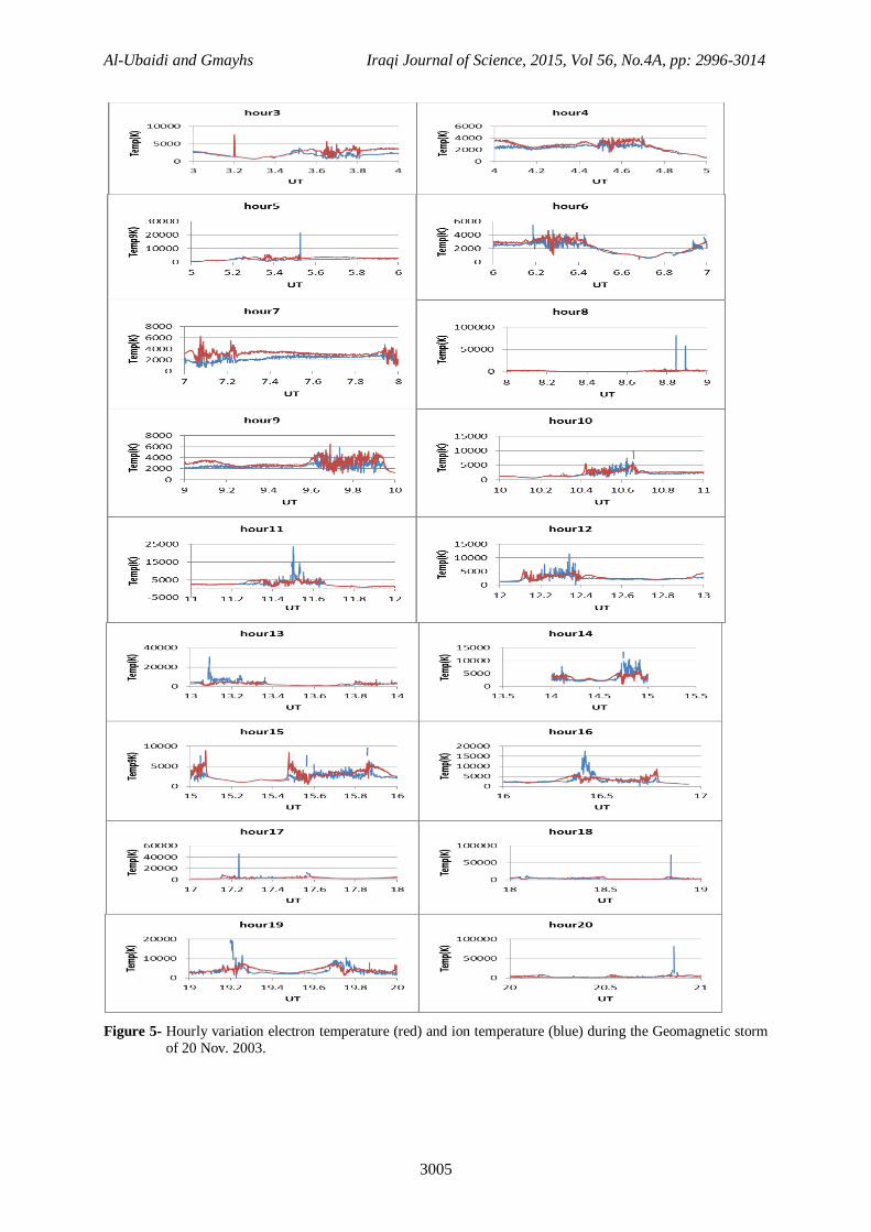
Figure 5- Hourly variation electron temperature (red) and ion temperature (blue) during the Geomagnetic storm
of 20 Nov. 2003.

Al-Ubaidi and Gmayhs Iraqi Journal of Science, 2015, Vol 56, No.4A, pp: 2996-3014
3006
Figure 6- Hourly variation electron temperature (red) and ion temperature (blue) during the Geomagnetic storm
of 8 Nov. 2004.

Al-Ubaidi and Gmayhs Iraqi Journal of Science, 2015, Vol 56, No.4A, pp: 2996-3014
3007
Figure 7- Hourly variation electron temperature (red) and ion temperature (blue) during the Geomagnetic storm
of 15 May 2005.

Al-Ubaidi and Gmayhs Iraqi Journal of Science, 2015, Vol 56, No.4A, pp: 2996-3014
3008
Figure 8- Hourly variation electron temperature (red), ion temperature (blue) and plasma velocity (green) during
the geomagnetic storm peak hours of 31 Mar 2001.

Al-Ubaidi and Gmayhs Iraqi Journal of Science, 2015, Vol 56, No.4A, pp: 2996-3014
3009
Figure 9- Hourly variation electron temperature (red), ion temperature (blue) and plasma velocity (green) during
the geomagnetic storm peak hours from 29-30 Oct. 2003.
Figure 10- hourly variation electron temperature (red), ion temperature (blue) and plasma velocity (green) during the geomagnetic storm peak hours from 31 Oct. 2003.

Al-Ubaidi and Gmayhs Iraqi Journal of Science, 2015, Vol 56, No.4A, pp: 2996-3014
3010
Figure 11- Hourly variation electron temperature (red), ion temperature (blue) and plasma velocity (green)
during the geomagnetic storm peak hours from 8 Nov. 2004.
Figure 12- Hourly variation electron temperature (red), ion temperature (blue) and plasma velocity (green)
during the geomagnetic storm peak hours from 15 May 2005.

Al-Ubaidi and Gmayhs Iraqi Journal of Science, 2015, Vol 56, No.4A, pp: 2996-3014
3011
Figure 13- Electron and ion temperature with latitude

Al-Ubaidi and Gmayhs Iraqi Journal of Science, 2015, Vol 56, No.4A, pp: 2996-3014
3012
Figure 14- Observed (solid) and predicted (dash) of Te (red) and Ti (blue) values.
Results and Discussion:
From data analysis it’s found that there are four branches that we can discuss, these are:-
a. Electron and ion temperature variation From figures 3-7, in general the temperature of the electron is greater than the temperature of the
ion, but there are some disturbances happened during the storm time, its seen that in year 2001
there was (7) severe and great storms happened in which the electron temperature has greater values than the ion temperature before the storm. In storm day, it is changed in the day and night
there is fluctuation in values of Te and Ti or there is a disturbances in temperature during the
storm time, Ti greater than Te in (31/3/2001) there is three severe and great events, the Ti peaks
hours seen from figure 3 are (4.34, 7.8, 9.5, 10.45, 11.3, 13.1, 13.1, 13.9, 14.7, 15.45, 16.25, 17.98, 19.1, 19.6, 21.3, 23-23.2). For other storms continues to the same behavior, related to the
storm happened in 2003 in day (29/10/2003) figure 4, it seen a peak Ti in hours (1.55, 2.55, 4.25,
6, 6.77, 8.7, 9.3, 10.2, 11.1-11.2, 12.2, 13.65, 14.56, 15.3-15.4, 16.2, 16.35, 16.9-17.1, 18.6-18.7, 19.57, 20.2-20.3, 21.4, 21.9-22, 23.6), in day (20/11/2003) as in figure 5, Ti peak hour are (5.5,
6.2, 8.86-8.9, 10.6, 11.5, 11.5, 12.2-12.4, 13.1, 14.7-15, 15.6-15.8, 16.4, 17.22, 18.8, 19.2, 20.85).
In 2004 it reveals that there are many peaks of Ti value which is greater than Te as in figure 6, day (8/11/2004) Ti peak hours (2.5, 3.5, 4.26, 5.1-6.3, 7.1, 8.6, 9.61, 10.3-10.5, 11.3, 12.2, 13.9,
15.5-15.6, ). In year 2005 there is one event in one day (15/5/2005) shown in figure (7) Ti peaks
appeared at (1.1, 2.6, 3.4, 12.8, 13.57, 14.56, 15.3, 16.2, 17, 18.72, 19.6, 20.4, 21.1, 23, 23.8).
This means that the severe and great geomagnetic storms suffer changes in Te and Ti. Te and Ti do not depend on the strength of the geomagnetic storm (through the Dst index), for
example at hour 9 in 31/3/2001 the value of (Dst -387nT) the value of Ti approach 8000K, while
at hour 7 in 1/4/2001the value of (Dst -161nT) Ti approach 85000K. To discuss this point there

Al-Ubaidi and Gmayhs Iraqi Journal of Science, 2015, Vol 56, No.4A, pp: 2996-3014
3013
may be other factors which appeared during the storm which effect on the Te and Ti values like
the coronal mass ejection (CME), related to table 1, it’s found that the appearance of severe and
great storms increases with increasing SSN value.
b. Plasma velocity variation From Figures 8-12 it reveals that plasma velocity variation seems to have the same profile of Te
and Ti variation during the storm time. To reveal the relation between plasma velocity and
electron temperature figure-15 is drawn to represent that there is linear relation between them.
Figure 15- Plasma velocity with electron and ion temperature.
c. Latitude variation of Te and Ti
From figure 13 the variation of electron and ion temperature with latitude during severe and great
storms shows that as the latitude increases and reach the poles the temperature of ions increases starting from 50 degree northern and southern hemisphere reaches maximum values
approximately 80000K. The reason for this may be due to the absence of magnetic field near
poles.
d. Validity of IRI model To check the validity of IRI model for calculating the electron and ion temperature during the
great and severe storms, six days (for 24 hours) are selected in which the storms happened from
two years 2001 and 2003. Comparing the predicted Te and Ti values with observed one it’s found from figure 14 that the predicted values from IRI model are much less than the observed values
and the variation was nonlinear along 24 hours, from this we can say that the model must
corrected to these two kinds of storms.
Summary:
From data analysis and results we can conclude that, in general:
The temperature of the electron is greater than the temperature of the ion, then it begin to disturbs
during the storm time it show the same values, but in the day and night there is fluctuation in
values of Te and Ti, Ti greater than Te the value of Ti approach 60000K.
It is clear that, through the Dst index, Te and Ti do not depend on the strength of the geomagnetic
storm. Plasma velocity variation seems to be of the same profile of Te and Ti variation during the storm and there is a linear relation between plasma temperature and velocity.
The variation of electron and ion temperature with latitude during severe and great storms shows
that as the latitude increases and reaches the poles the temperature of ions increases starting from
50 degree northern and southern hemisphere reaches maximum values approximately 80000K.
To check the validity of IRI model for calculating the electron and ion temperature during the
great and severe storms, it’s found that the predicted values from IRI model much less than the
observed values and the variation was nonlinear along 24 hours.

Al-Ubaidi and Gmayhs Iraqi Journal of Science, 2015, Vol 56, No.4A, pp: 2996-3014
3014
Acknowledgments:
This work relates to Department Baghdad University/ College of Science/ Department of
Astronomy and Space. The data are provided from (DMSP) for plasma, NASA for whom I would like
to introduce my utmost appreciation and thanks. The authors also acknowledge the use of index data from World Data Center for Geomagnetism, Kyoto, and NASA/SPDF and geophysics data from UK
wdc.
References:
1. Schunk, R. and Nagy, A.F. 2009. Ionospheres: Physics, Plasma Physics, and Chemistry.
Cambridge Atmospheric and Space Science Series, Cambridge University Press. 2. Stubbe, P. and Hagfors, T. 1997. The Earth’s Ionosphere. A Wall-less Plasma Laboratory, Surv.
Geophys, 18:57-127.
3. Schunk, R.W. Nagy, A.F. 2009. Ionospheres. 2nd edition Cambridge University Press,
Cambridge, UK. 4. David, M. Schunk, R.W. Sojka, J.J. 2011. The effect of downward electron heat flow and electron
cooling processes in the high-latitude ionosphere. Journal of Atmospheric and Solar-Terrestrial
Physics, 73:2399–2409. 5. Buonsanto, M.J. 1989. Comparison of incoherent scatter observations of electron density, and
electron and ion temperature at Millstone Hill with the International Reference Ionosphere.
Journal of atmospheric and Terrestrial Physics, 51(5):441-468.
6. Forme, F.R.E. Wahlund, J.-E. Opgenoorth, H.J. Persson, M.A.L. Mishin, E.V. 1993. Effects of current driven instabilities on the ion and electron Temperature in the topside ionosphere. Journal
of Atmospheric and Terrestrial Physics, 55(4/5):611-666.
7. Pavlov, A.V. Abe, T. Oyama, K.-I. 2001. Comparison of the measured and modeled electron densities and temperatures in the ionosphere and plasmasphere during the period 25–29 June
1990. Journal of Atmospheric and Solar-Terrestrial Physics, 63:605–616.
8. Sethi, N. Pandey, V. Mahajan, K. 2004. Seasonal and solar activity changes of electron temperature in the F-region and topside ionosphere. Advances in Space Research, 33:970–974.
9. Gulyaeva, T.L. and Titheridge,J.E. 2006. Advanced specification of electron density and
temperature in the IRI ionosphere–plasmasphere model. Advances in Space Research, 38:2587–
2595. 10. Jiuhou Lei, Raymond, G. Roble, Wenbin Wang, Barbara, A. Emery, Shun-Rong Zhang. 2007.
Electron temperature climatology at Millstone Hill and Arecibo. Journal of geophysical research,
112, A02302, doi:10.1029/2006JA012041. 11. Klimenko, M.V. Klimenko, V.V. Bryukhanov, V.V. 2008. Numerical modeling of the light ion
trough and heat balance of the topside ionosphere in quiet geomagnetic conditions. Journal of
Atmospheric and Solar-Terrestrial Physics, 70: 2144–2158.
12. Schunk, R.W. and Nagy, A.F. 2010. Electron temperatures in the F region of the ionosphere. Advances in Space Research, 16: 255-399.
13. Ewa Slominska and Hanna Rothkaehl. 2013. Mapping seasonal trends of electron temperature in
the topside ionosphere based on DEMETER data. Advances in Space Research,52: 192–204. 14. deMeneses, F.C. Klimenko, M.V. Klimenko, V.V. AlamKherani, E. Muralikrishna, P. JiyaoXu,
Hasbi, A.M. 2013. Electron temperature enhancements in nighttime equatorial ionosphere under
the occurrence of plasma bubbles. Journal of Atmospheric and Solar-Terrestrial Physics, 103:36-47.
15. Duboin, N. L. and Kamide, Y. 1984. Latitudinal variations of Joule heating due to the
auroralelectrojets.Geophys, 89:245-251.
16. Hays, P. Jones, R. and Rees, M. 1973. Auroral heating and the composition of the neutral atmosphere. Planet Space and Scienc, 21:559-573.
17. Anita Aikio. 2011. Introduction to the ionosphere. University of Oulu, Finland.
18. Loewe, C. A. and Prölss, G. W. 1997. Classification and mean behaviour of magnetic storms. Journal Geophysical Research, 102: 14209-14213.
19. Bilitza, D. 2001. International Reference Ionosphere 2000. Radio Science, 36:261-275.
20. Bilitza, D. 2003. International Reference Ionosphere 2000 examples of improvement and new features. Advances in Space Research, 31:151–167.