DCSP-12: Filter II

Jianfeng Feng

Department of Computer Science Warwick Univ., UK

Jianfeng.feng@warwick.ac.uk

http://www.dcs.warwick.ac.uk/~feng/dcsp.html

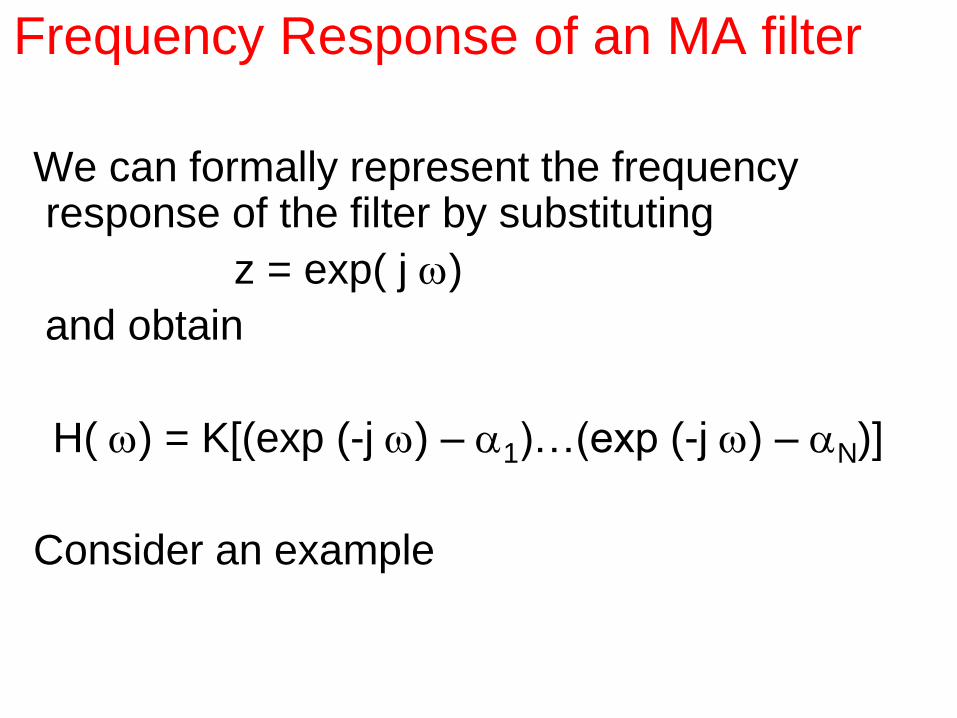
Frequency Response of an MA filter

We can formally represent the frequency response of the filter by substituting

z = exp( j w)

and obtain

H( w) = K[(exp (-j w) – a1)…(exp (-j w) – aN)]

Consider an example

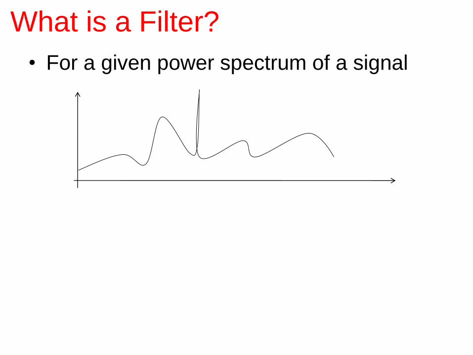
What is a Filter?

• For a given power spectrum of a signal

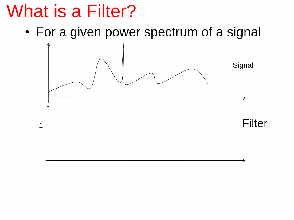
What is a Filter?• For a given power spectrum of a signal

Signal

Filter1

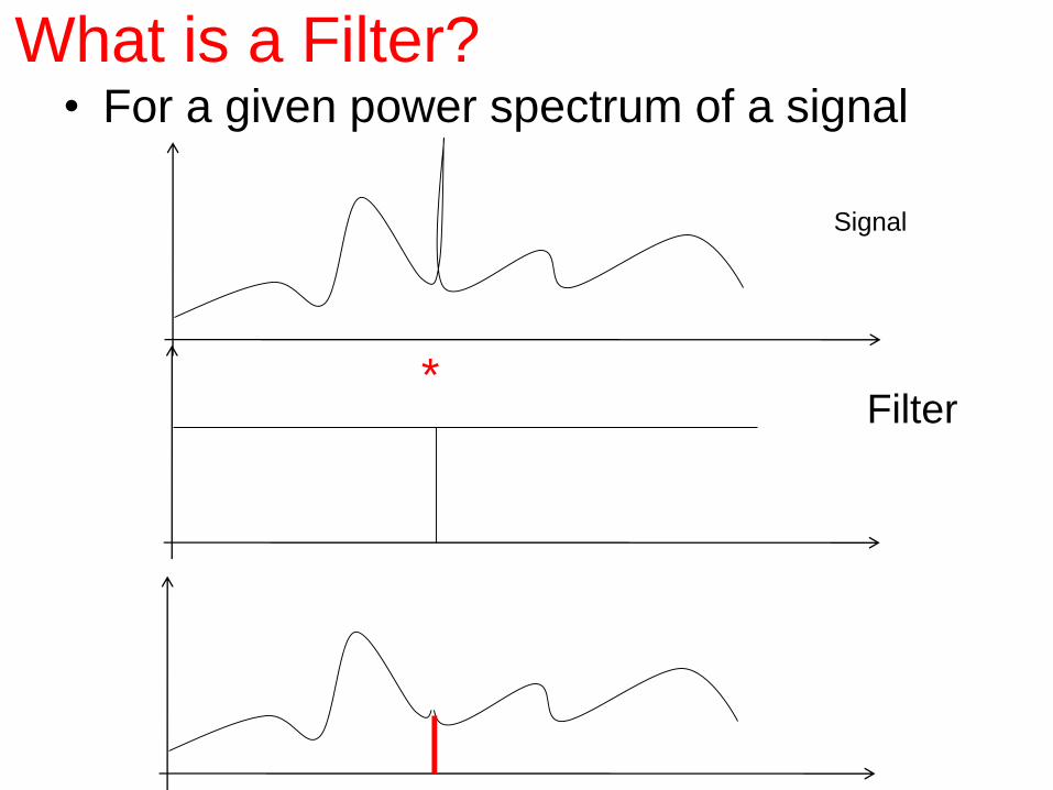
What is a Filter?• For a given power spectrum of a signal

1

Filter

Signal

*

Filtered Signal

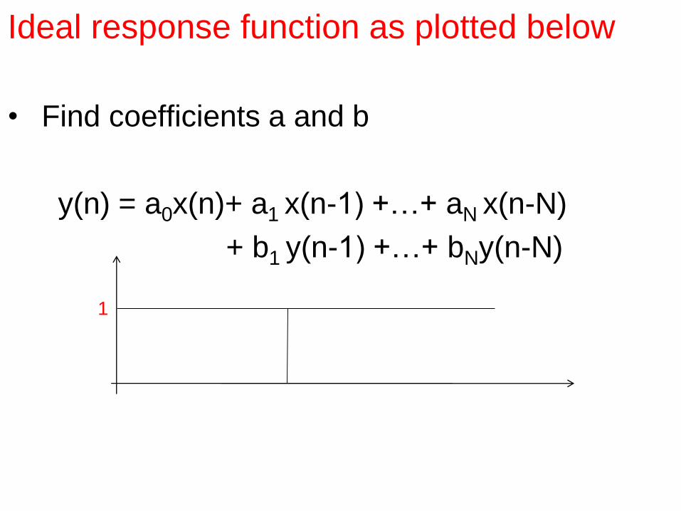
Ideal response function as plotted below

• Find coefficients a and b

y(n) = a0x(n)+ a1 x(n-1) +…+ aN x(n-N)

+ b1 y(n-1) +…+ bNy(n-N)

1 Filter

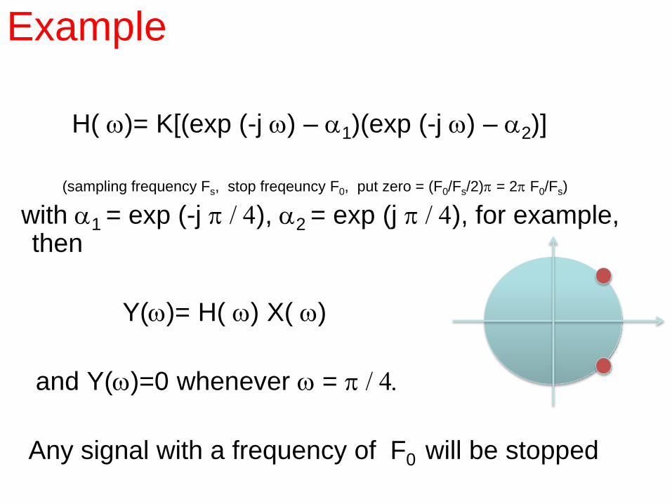
Example

H( w)= K[(exp (-j w) – a1)(exp (-j w) – a2)]

(sampling frequency Fs, stop freqeuncy F0, put zero = (F0/Fs/2)p = 2p F0/Fs)

with a1 = exp (-j p / 4), a2 = exp (j p / 4), for example, then

Y(w)= H( w) X( w)

and Y(w)=0 whenever w = p / 4.

Any signal with a frequency of F0 will be stopped

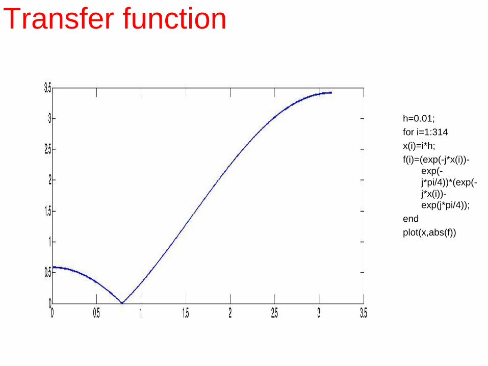
Transfer function

h=0.01;

for i=1:314

x(i)=i*h;

f(i)=(exp(-j*x(i))-

exp(-

j*pi/4))*(exp(-

j*x(i))-

exp(j*pi/4));

end

plot(x,abs(f))

Moving a1 along the circle, we are able to stop a signal with a given frequency

Transfer function

p/4

p/3

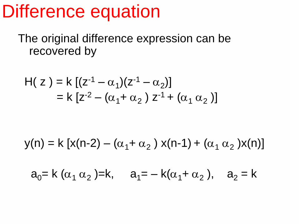
The original difference expression can be recovered by

H( z ) = k [(z-1 – a1)(z-1 – a2)]

= k [z-2 – (a1+ a2 ) z-1 + (a1 a2 )]

y(n) = k [x(n-2) – (a1+ a2 ) x(n-1) + (a1 a2 )x(n)]

a0= k (a1 a2 )=k, a1= – k(a1+ a2 ), a2 = k

Difference equation

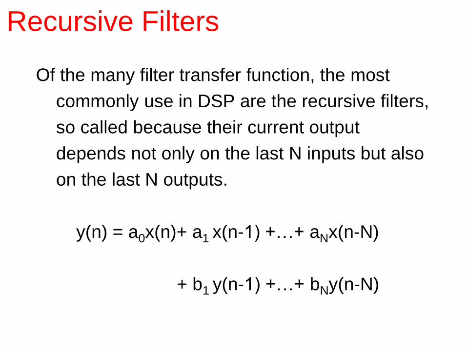
Recursive Filters

Of the many filter transfer function, the most

commonly use in DSP are the recursive filters,

so called because their current output

depends not only on the last N inputs but also

on the last N outputs.

y(n) = a0x(n)+ a1 x(n-1) +…+ aNx(n-N)

+ b1 y(n-1) +…+ bNy(n-N)

Transfer function

H (z) =A(z)

B(z)

where

A(z) = a0 + a1z-1 +...+ aNz

-N

B(z) =1- b1z-1 -... - bNz

-N

ìíï

îï

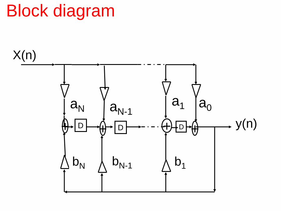
X(n)

aN

D D

aN-1

+

a0

y(n)+

bN bN-1

a1

b1

++

Block diagram

D

Poles and zeros

• We know that the roots an are the zeros of the transfer function.

• The roots of the equation B(z)=0 are called the poles of the transfer function.

• They have greater significance for the behaviour of H(z): it is singular at the points z = bn.

• Poles are drawn on the z-plane as crosses, as shown in the next Fig.

H (z) =A(z)

B(z)=

(z -ai )i=1

N

Õ

(z - bi )i=1

N

Õ

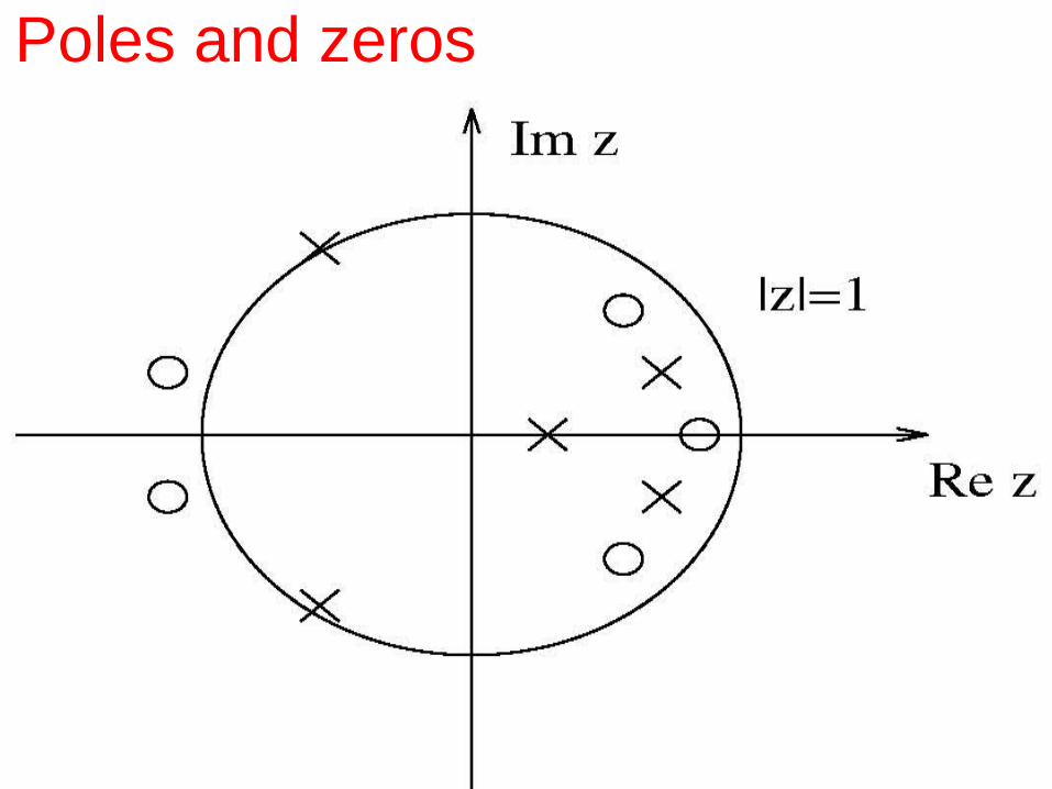
Poles and zeros

ON this figure, the unit circle has been shown on the z-plane.

In order for a recursive filter to be bounded input bounded output (BIBO) stable, all of the poles of its transfer function must lie inside the unit circle.

A filter is BIBO stable if any bounded input sequence gives rise to a bounded output sequence.

Now if the pole of the transfer lie insider the unit circle,

A simple case (N=1)

Poles and zeros

H (z) = k(z)

(z- b)=

k

(1- bz-1)

y(n) = by(n-1)+ kx(n)

ì

íï

îï

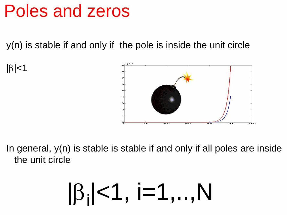
Poles and zeros

y(n) is stable if and only if the pole is inside the unit circle

|b|<1

In general, y(n) is stable is stable if and only if all poles are inside

the unit circle

|bi|<1, i=1,..,N

If |bi |=1, the filter is said to be conditionally stable:

some input sequence will lead to bounded

output sequence and some will not.

Since MA filters have no poles, they are always

BIBO (bound input bound output) stable: zeros

have no effect on stability.

Poles and zeros

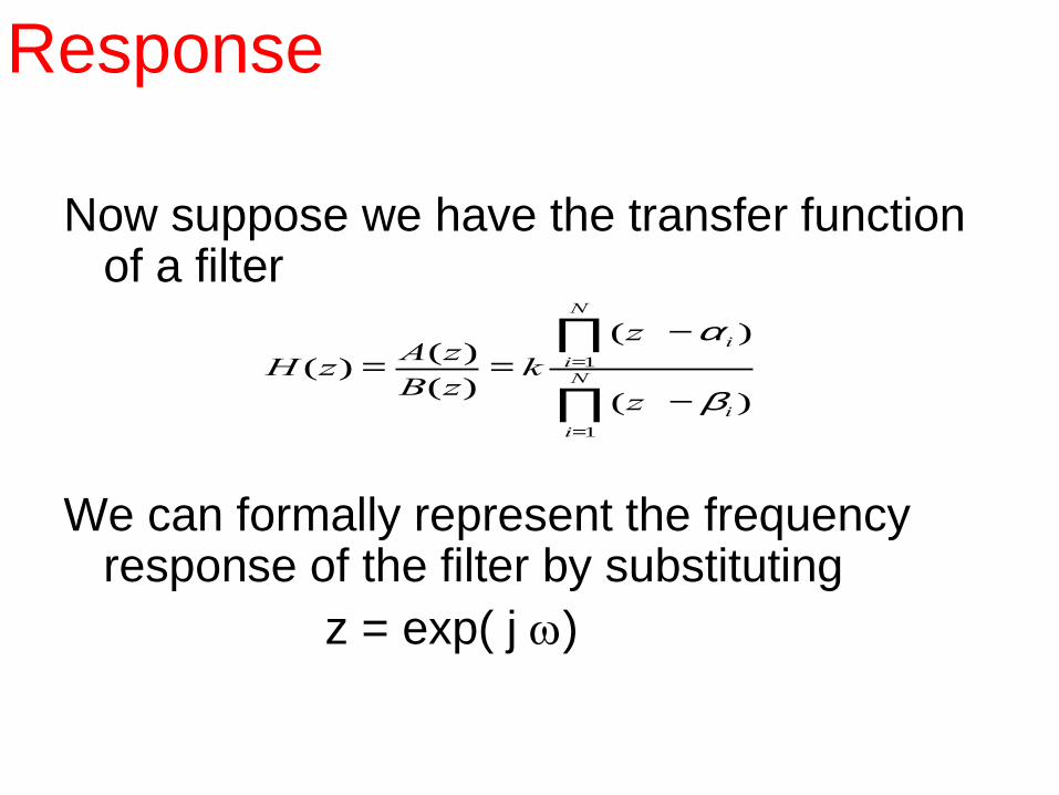
Response

Now suppose we have the transfer function of a filter

We can formally represent the frequency response of the filter by substituting

z = exp( j w)

and obtain

H( w)= A( w ) / B( w )

H (z) =A(z)

B(z)= k

(z -ai )i=1

N

Õ

(z - bi )i=1

N

Õ

Response

Obviously, H( w) depends on the locations of

the poles and zeros of the transfer function,

a fact which can be made more explicit by

factoring the numerator and denominator

polynomials to write

H (w) =A(w)

B(w)= k

(exp( jw) -ai )i=1

N

Õ

(exp( jw) - bi )i=1

N

Õ

Each factor in the numerator or denominator

is a complex function of frequency, which

has a graphical interpretation in the terms

of the location of the corresponding roots

in relation to the unit circle

Thus we can make a reasonable guess

about the filter frequency response imply

by looking at the pole-zero diagram.

Response

There are four main classes of filter in widespread use:

filters.

The name are self-explanatory

This four types are shown in the next figure

Filter Types

• Lowpass

• highpass

• bandpass

• bandstop

Filter Types

DCSP-13: Simple Filter

Jianfeng Feng

Department of Computer Science Warwick Univ., UK

Jianfeng.feng@warwick.ac.uk

http://www.dcs.warwick.ac.uk/~feng/dcsp.html

A bit fun today

Google’s AI AlphaGo to take on world No 1 Lee Se-dol in live broadcast

DeepMind’s Go-playing software will play South Korean in five-match game live-streamed

on YouTube, following victory over European champion

Applications of filter

HumanEar.jpg

Frequency

band [f1 f2]

Frequency

band [f3 f4]

Applications of filter

simple filter design

• In a number of cases, we can design a

linear filter almost by inspection.

• moving poles and zeros like pieces on a

chessboard.

simple filter design

• This is not just a simple exercise designed

for an introductory course

• For in many cases the use of more

sophisticated techniques might not yield a

significant improvement in performance.

• In this example consider the audio signal s(n), digitized with a sampling frequency Fs (12kHz).

simple filter design

• In this example consider the audio signal s(n), digitized with a sampling frequency Fs (12kHz).

• The signal is affected by a narrowband (i.e., very close to sinusoidal) disturbance w(n).

simple filter design

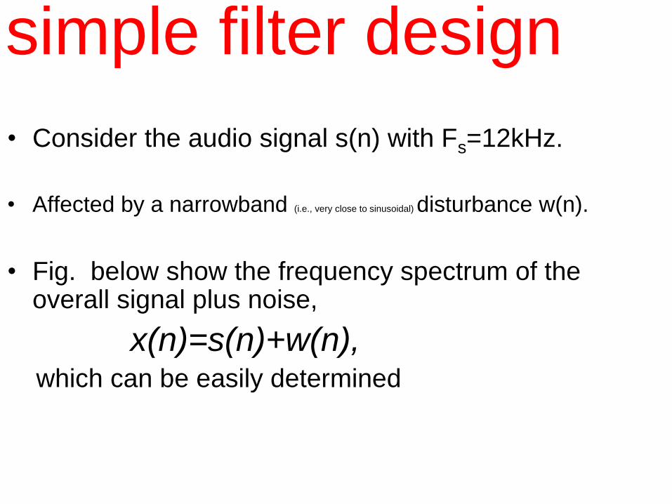
• Consider the audio signal s(n) with Fs=12kHz.

• Affected by a narrowband (i.e., very close to sinusoidal) disturbance w(n).

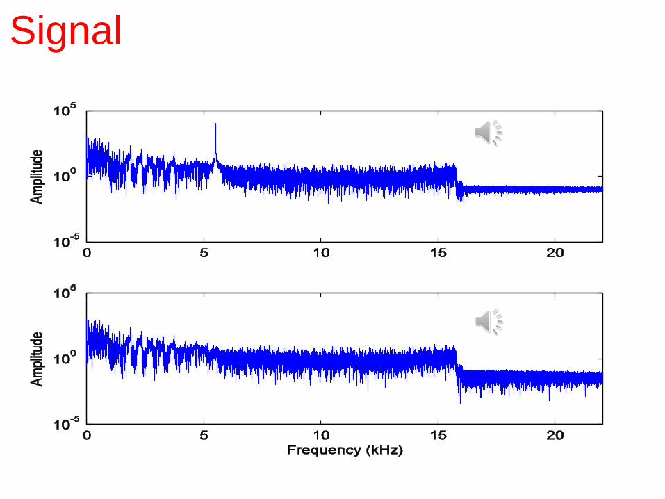
• Fig. below show the frequency spectrum of the overall signal plus noise,

x(n)=s(n)+w(n), which can be easily determined.

simple filter design

Signal

• Notice two facts:

• The signal has a frequency spectrum within the interval 0 to Fs/2 kHz.

• The disturbance is at frequency F0 (1.5) kHz.

• Design and implement a filter that rejects

the disturbance without affecting the signal excessively.

• We will follow three steps:

simple filter design

Step 1: Frequency domain specifications

• Reject the signal at the frequency of the disturbance.

• Ideally, we would like to have the following frequency response:

where w0=2p (F0/Fs) = p/4 radians, the digital frequency

of the disturbance.

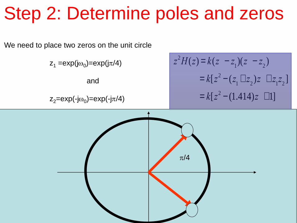
Step 2: Determine poles and zeros

We need to place two zeros on the unit circle

z1 =exp(jw0)=exp(jp/4)

and

z2=exp(-jw0)=exp(-jp/4)

z2H (z) = k(z - z1)(z - z

2)

= k[z2 - (z1+ z

2)z + z

1z

2]

= k[z2 - (1.414)z +1]

p/4

Step 2: Determine poles and zeros

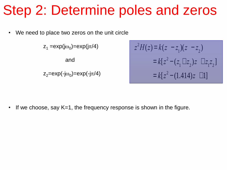
• We need to place two zeros on the unit circle

z1 =exp(jw0)=exp(jp/4)

and

z2=exp(-jw0)=exp(-jp/4)

• If we choose, say K=1, the frequency response is shown in the figure.

z2H (z) = k(z - z1)(z - z

2)

= k[z2 - (z1+ z

2)z + z

1z

2]

= k[z2 - (1.414)z +1]

PSD and Phase

• As we can see, it rejects the desired frequency

• As expected, but greatly distorts the signal

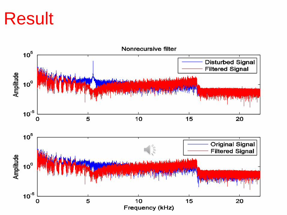
Result

• A better choice would be to select the poles close to the zeros, within the unit circle, for

stability.

• For example, let the poles be p1= r exp(jw0) and p2= r exp(-jw0).

• With r =0.95, for example we obtain the transfer function

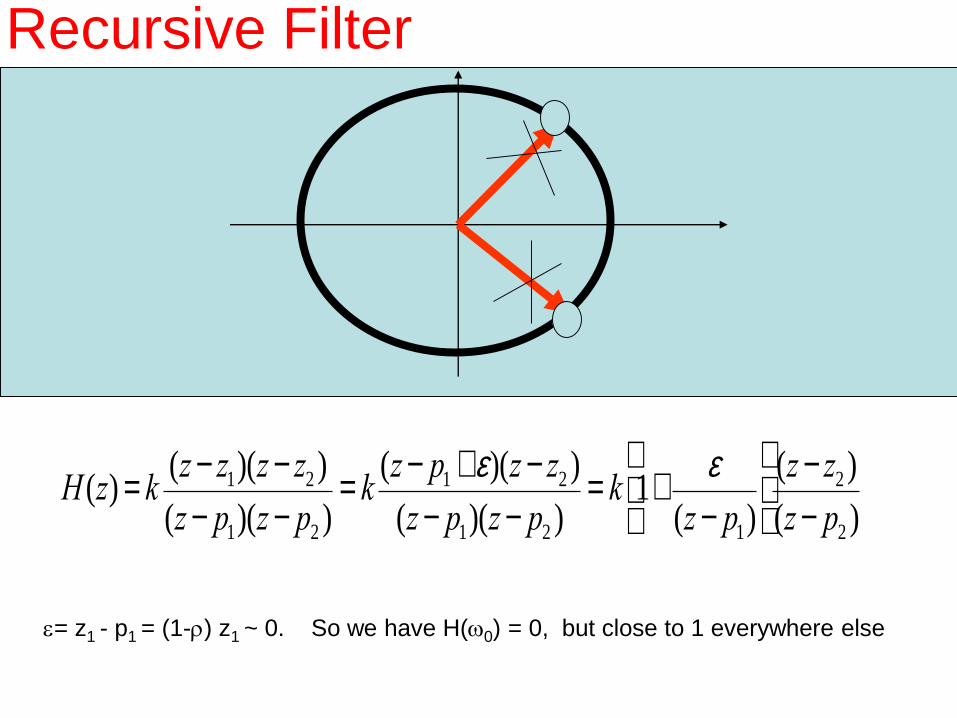
Recursive Filter

H (z) = k(z- z1)(z- z2 )

(z- p1)(z- p2 )

Recursive Filter

H(z) = k(z- z1)(z- z2 )

(z- p1)(z- p2 )= k

(z- p1 +e)(z- z2 )

(z- p1)(z- p2 )= k 1+

e

(z- p1)

æ

èç

ö

ø÷

(z- z2 )

(z- p2 )

e= z1 - p1 = (1-r) z1 ~ 0. So we have H(w0) = 0, but close to 1 everywhere else

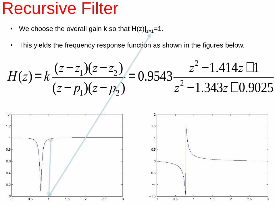
• We choose the overall gain k so that H(z)|z=1=1.

• This yields the frequency response function as shown in the figures below.

H(z) = k(z- z1)(z- z2 )

(z- p1)(z- p2 )= 0.9543

z2 -1.414z+1

z2 -1.343z+0.9025

Recursive Filter

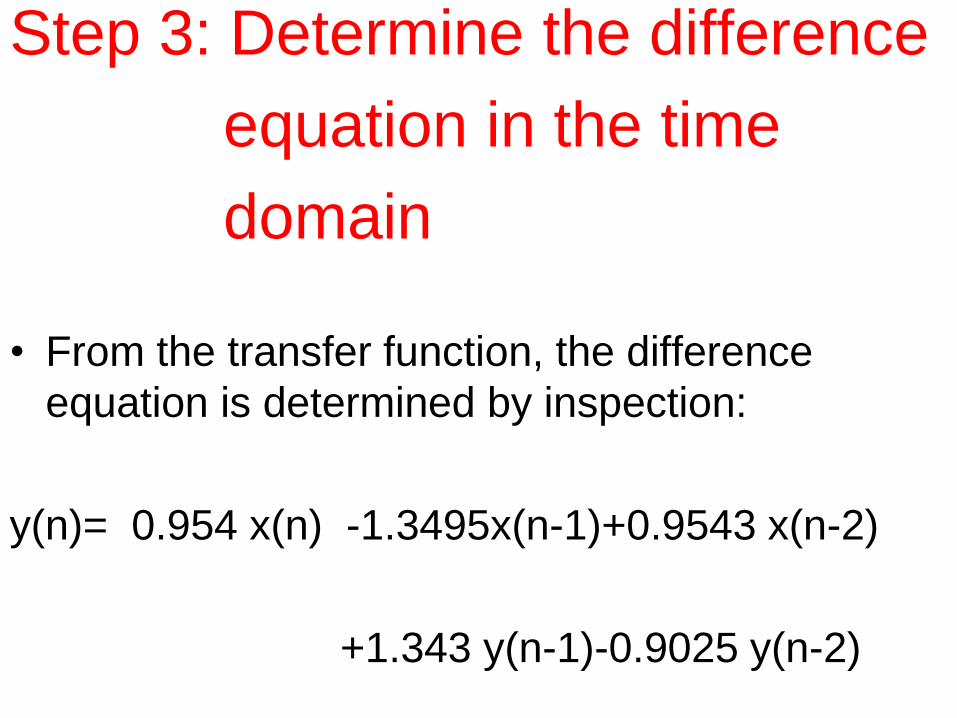
Step 3: Determine the difference

equation in the time

domain

• From the transfer function, the difference

equation is determined by inspection:

y(n)= 0.954 x(n) -1.3495x(n-1)+0.9543 x(n-2)

+1.343 y(n-1)-0.9025 y(n-2)

• Easily implemented as a recursion in a high-level language.

• The final signal y(n) with the frequency spectrum shown in the

following Fig.,

• We notice the absence of the disturbance.

Step 3: difference equation

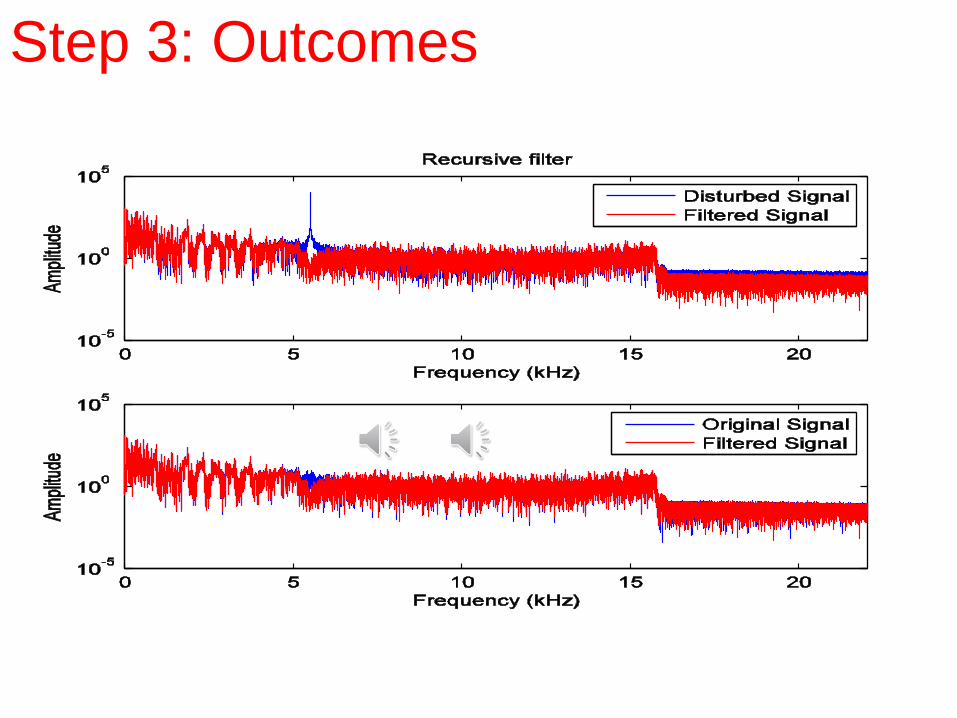
Step 3: Outcomes

demo

\Program Files\MATLAB71\work

simple_filter_design

soundsc(s,Fs)

soundsc(x,Fs)

soundsc(y,Fs)

soundsc(yrc,Fs)

General Filter Design

• Using Chebyshev or Butterworth

polynomials to approximate a square wave

function in the frequency domain

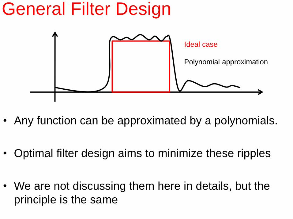
• Any function can be approximated by a polynomials.

• Optimal filter design aims to minimize these ripples

• We are not discussing them here in details, but the

principle is the same

Ideal case

Polynomial approximation

Next week

• Some further funs

Matched filter (radar for example)

Wiener filter (get rid of white noise)

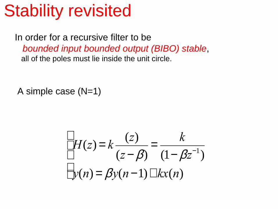
In order for a recursive filter to be

bounded input bounded output (BIBO) stable, all of the poles must lie inside the unit circle.

A simple case (N=1)

Stability revisited

H (z) = k(z)

(z- b)=

k

(1- bz-1)

y(n) = by(n-1)+ kx(n)

ì

íï

îï

Stability revisited

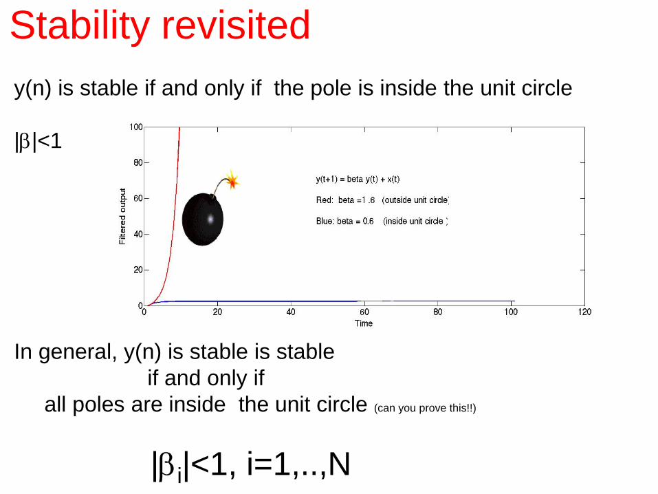
y(n) is stable if and only if the pole is inside the unit circle

|b|<1

In general, y(n) is stable is stable

if and only if

all poles are inside the unit circle (can you prove this!!)

|bi|<1, i=1,..,N