dealing in junk: money makers or money takers? · fuxun xia & wayron lewis dealing in junk:...

ASSA CONVENTION 2012, CAPE TOWN, 16–17 OCTOBER 2012 | 337

DEALING IN JUNK: MONEY MAKERS OR MONEY TAKERS?

By Fuxun Xia and Wayron Lewis

Presented at the Actuarial Society of South Africa’s 2012 Convention16–17 October 2012, Cape Town International Convention Centre

ABSTRACTA study of historical default rates of firms issuing high-yield bonds in the US is undertaken in this paper. A multivariate logistic regression analysis is undertaken and results in the development of five models which incorporate financial ratios and variables to predict default by such firms. We find that firms with relatively lower total assets, earnings before interest and tax and cash flows from operating activities are more prone to default on their debt obligations. Hence, the financial ratios including these factors tend to be significant in the models. The study proceeds to examine the effect on default rates by macro-economic factors in conjunction with financial ratios and variables previously used. We conclude that macro-economic factors are dominant in determining default over the long term. Lastly the smaller South African high-yield debt market is examined and its relevance in the context of the study is determined.

KEYWORDSDefault; multivariate logistic regression; financial ratios and variables; macro-economic factors; bonds; junk; high yield

CONTACT DETAILSFuxun Xia, E-mail: [email protected]; Tel: +27(0)82 341 9894Wayron Lewis, Email: [email protected]; Tel: +27(0)78 422 5388

338 | FUXUN XIA & WAYRON LEWIS DEALING IN JUNK: MONEY MAKERS OR MONEY TAKERS?

ASSA CONVENTION 2012, CAPE TOWN, 16–17 OCTOBER 2012

1. INTRODUCTIONWith a South African high-yield market that is in its infancy, junk bonds are a potentially viable new asset class for individuals and institutions alike. The financial crisis of 2009 brought to light the potentially devastating consequences to investors’ funds when indicators of impending danger are ignored. The elevated risk associated with high-yield bonds would then naturally cause the individual investor considerable nervousness if there were not a way to quantify at least some of the risk involved. Therefore predictive default probabilities of companies issuing high-yield debt could go a long way in aiding investors take sensible, calculated risks and still get a good night’s sleep. The particular interest in attempting to model default probability on high-yield bonds is obvious when the benefit of having a measure of certainty for the possibility of high return is considered. Armed with the right tools, an investor could capitalise on the potential growth the South African high-yield market is likely to experience in the near future.

2. BACKGROUNDHigh-yield bonds, also known as junk bonds or speculative grade bonds, are corporate loan stock that are issued by companies with a Moody’s credit rating of Ba1 or lower or a Standard & Poor’s rating of BB+ or lower. As such, these companies are more prone to default or delay on the coupon or capital payments of the bond, thus, junk bonds have greater yields than conventional or investment grade bonds to compensate for the higher risk. Additionally, high-yield debts are subordinate to conventional debt so buyers of junk bonds are second in line behind other creditors if bankruptcy occurs. Offering high yields on bonds issued by such companies is often the only choice they have as a means of attracting investors and raising capital.

The majority of issued junk bonds are located in the US. Historically, the spread of a junk bond from US Treasury bonds ranges from 3% to 9% with an average of 6% (Yago, n.d.).

Junk bonds are available to investors directly or via a collective investment scheme that specialises in producing high returns. The junk bond market was worth about $1 trillion in the US in 2006 (NYU Salomon Center, 2006).

3. OBJECTIVEThe objective of this study is to develop a comprehensive model utilising financial ratios and variables which were used in an array of previous studies such as Altman (1968), Huffman and Ward (1996) and Bryan, Marchesini and Perdue (2004) for the purpose of predicting the probability that a firm with junk bonds will default given information one and two years prior to default respectively. We shall then attempt to integrate the model with macro-economic factors that can predict default regardless of the state of the economy in any given year. We intend to examine if the models can be of use to an investor with the intention of investing in the South African high-yield debt market.

FUXUN XIA & WAYRON LEWIS DEALING IN JUNK: MONEY MAKERS OR MONEY TAKERS? | 339


4. THE HISTORY OF HIGH-YIELD BONDSJunk bonds originated in the United States in the early 20th century. Companies such as General Motors and IBM issued high-yield bonds for financing during that period. However, junk bonds as a whole were never popular in the market at that time. Before the 1980s, all new bonds issued were conventional investment grade bonds and the only junk bonds that were available to trade were issued by companies that originally had a safe credit rating but subsequently became more prone to default which downgraded their bonds to junk status. These bonds were called “fallen angels”. The coupon payments of the fallen angels were similar to other investment grade bonds but they could be bought at such a discount that the resulting yield was remarkably high.

Before the 1970s, exchange rates in the US followed the Bretton Woods system which caused it to remain relatively steady. The system collapsed in 1971 and subsequently caused a rising of inflation and interest rates. Simultaneously, the US experienced a recession. As a result, banks only lent money to large blue-chip companies. Only the safest companies could receive credit and the companies most in need of capital, the growing companies, could not have access for financing. This brought about a boom of the high-yield bond market in the 1980s. Issuing bonds with high-yields was the only option for companies to raise capital. In 1977 newly-issued junk bonds appeared for the first time in several years.

In the 1980s, underwriting of junk bonds was synonymous with a trader named Michael Milken working at Drexel Burnham Lambert. Milken realised that, despite the high default risk, junk bonds were actually undervalued. He began encouraging investors and companies to buy and issue high-yield bonds and created huge demand for them. New junk bond issuance grew from $839 million in 1981 to $8.5 billion in 1985 to $12 billion in 1987. Junk bonds became 25% of the corporate bond market (Lewis, 1989). This new demand for high-yield bonds created problems of supply. There was not enough supply of junk bonds available for investment to absorb investors’ cash. Milken found solutions to the problem. One of his tactics was using high-yield debt for leveraged buyouts (LBO). Money raised from issuing junk bonds was used to acquire control over another undervalued company. Once that company was acquired, the cash flows of that company were used to pay the coupons of the bond. Additionally, since the acquired company possessed more debt via the junk bonds, its own credit rating plummeted and its own bonds transformed into new fallen angels.

In 1989, a recession hit and several firms defaulted on their junk bonds. Milken was arrested due to fraud and Drexel Burnham Lambert went to the verge of bankruptcy. This caused a collapse in the high-yield market.

The market recovered in the 1990s. Due to tighter regulations, junk bonds became more stable and acted just like any other asset classes. LBOs were no longer possible using junk bonds. Returns averaged 15% annually and default rates were as low as an average of 2.4% during the period (Yago, n.d.).

The market suffered another setback from 2000 to 2002 when high default rates were present. The average annual return was 0% as a result. (Yago, n.d.)



In the 21st century, junk bonds began to have global appeal. In Europe, the market for junk bonds has been growing steadily with issues worth 50 billion euros in 2010 (Sakoui, 2010).

South African companies began issuing high-yield bonds for capital in 2005. The market in South Africa is worth about R1.5 billion with projections of it increasing tenfold in the next five years. The yield of junk bonds in South Africa typically has a spread from 3.5% to 7% compared to the 3-month Johannesburg Interbank Agreed Rate (JIBAR) (Theunissen, 2010).

5. LITERATURE REVIEW5.1 Previous Relevant StudiesThere has been an increase in the necessity of and interest in predicting financial distress in corporations ever since the initial research by Altman (1968). He developed a multivariate model to predict corporate bankruptcy based on discriminant analysis using a combination of financial and accounting ratios, building on the research of Beaver (1966). He was the first person to use the statistical technique of discriminant analysis for the purpose of classifying corporate failure. It was developed into what is known today as the Z-score model. Altman later improved upon the model to create the now trademarked Zeta analysis model.

The resultant studies have naturally led to other applications of the theory, such as the study of default on corporate bonds.

Asquith, Gertner and Scharfstein (1994) explored the way in which firms in financial distress avoid bankruptcy and default. They found that the main ways through which firms avoid bankruptcy is through bank and public debt restructuring, asset sales, reducing capital expenditure, mergers and layoffs. They found that asset sales, as a way to avoid bankruptcy, are limited by the industry that the firm is in. They found that for companies that issue high-yield debt, the structure of the junk bond has implications for the likelihood of default when the firm becomes financially distressed. While the level of debt was traditionally regarded as the key variable affecting costs of financial distress, their analysis concluded that the debt composition in those cases also determines if financial distress leads to default or not.

Hilscher and Wilson (2010) explored the relevance of credit ratings as a pure predictor of the probability of default of a firm. They found that simple models derived from publicly available financial statements can easily surpass the predictive powers of a credit rating. They theorised that the ratings are more representative of the state of a company at a particular time in the economy and that changes in the economy can more likely change a rating than a company actually improving its financial situation. They conclude that rating agencies do not have the sole objective of making accurate default probability forecasts through their ratings. Additionally, as rating agencies respond slowly to new information, use of credit ratings as a predictor of default should be regarded sceptically.

Beaver (1966) explored the possibility of using a single financial ratio from a



company to determine its likelihood of default. He also noted the discrepancy in asset sizes between defaulted and non-defaulted firms. Additionally non-defaulted firms experienced higher growth. He noted that conventional ratios such as current ratios were not good predictors which hints at firms appearing to “window dress” the ratios most commonly examined. He concluded that financial ratios when used singularly can have high predictive power of solvency for at least five years prior to failure. He also speculated that a multivariate analysis might enhance his univariate results.

Hakim and Shimko (1995) undertook a study of the influence on high-yield bond defaults by firms’ characteristics. A firm’s credit rating, cash flow, market value, long-term debt and investment activity are used to build a model for the purpose of quantifying the probability of the firm defaulting on its bonds. A fall in cash flows may be indicative of financial difficulties and the accompanying consequences. They believe that a company perceived to have high default risk will issue a high portion of long-term debt in order to service their current debt obligations and gain more time in which to better their current position. They propose that an increase in a firm’s overall risk will be accompanied by an increase in investment activity by that firm in an attempt to achieve the prior state of financial stability and, as a way of encapsulating the remaining risk, the market value of the firm is employed. Hakim and Shimko(1995) reach the conclusion that default by firms on their (junk) bond issues are more likely when the firm is experiencing a decline in market value, has a high level of variation in long-term debt and a small margin of cash flow.

Huffman and Ward (1996) developed a methodology for predicting default for high-yield bonds based on public information available at the time of issue. Multivariate logistic regression analysis is used (as opposed to discriminant analysis) in the study to determine the significance that different factors have towards the likelihood of default on the bonds. Shortcomings of Altman’s original research are highlighted when applied to their framework, such as the tendency for his model to predict a defaulting bond when in fact it does not default. The implication of the conclusion by Huffman and Ward (1996) is that investors should use default prediction models as opposed to bankruptcy prediction models as a useful tool in selecting risky bond portfolios. They determined that the cash flows of a company are the most significant factor affecting default of high-yield bonds.

Bryan, Marchesini and Perdue (2004) enhanced Huffman and Ward’s study and introduced a new methodology to determine default rates. They introduced several new variables into their study and examined cash flow factors in unison with traditional financial ratios. They concluded that the integration of accounting ratios with cash flow measures provided higher predictive powers than any in isolation. They noted that macro-economic factors could have a significant impact on default rates as well but did not incorporate any in their model.

Helgewe and Kleiman (1996) discuss three factors that affect the aggregate default rates of high-yield bonds, namely: changes in the credit ratings of speculative-grade debt, the duration that debt has been outstanding, and the general state of the



economy. The adjusted R-square measure is used in a regression analysis to indicate the percentage of variation in aggregate default rates explained by the abovementioned factors. Helgewe and Kleiman (1996) suggest that according to statistical evidence, the distribution of credit ratings in the high-yield debt market at the beginning of the year will give a good indication of the aggregate default activity to be expected over the year. For example, a low concentration of poorly rated debt in the beginning of the year would be associated with a below-average number of defaults throughout the year and vice versa. It is also indicated that the cycles of issuance in the high-yield debt market seem to have a high correlation with the returns in the market and that the aging factor could very well be correlated with economic activity. A 13 percent increase to the adjusted R-squared is noted when GDP growth is included in their model as an indicator of the state of the economy. A conclusion is drawn that the three factors have significant influence in determining annual aggregate default rates in the high-yield debt market with credit quality being the most influential.

5.2 Other Methods of Predicting DefaultMerton (1974) proposed modelling default of a company in terms of exercising a derivative option. He characterised the equity of a company as a European call option on its assets. He drew similarities between whether or not a company can repay its debt to whether an option will be exercised or not. He used put-call parity to calculate the value of a put and that represents the risk of default of a company’s outstanding debt.

The Moody’s corporation has developed a propriety model called the Moody’s KMV (MKMV) model. It implements the Vasicek-Kealhofer(VK) model (which extends the classical Black-Scholes-Merton framework to model default probability) to calculate an Expected Default FrequencyTM (EDFTM) which is the probability of default for either the following year (or years) for companies with publicly traded equities (Bohn & Crosby, 2003). It has received much criticism from academics who have undertaken studies to examine the accuracy of the model under various circumstances.

Mirkin (2009) explored credit risk exposures and liquidity risk through the use of empirical data analysis of total return indices, credit spreads, volatilities and optimal portfolio estimation. He used several optimisation techniques to determine suitable risk adjusted discount rates to use for valuation of risky assets. He also examined the link between credit default swaps and the propensity of the underlying asset to default.

McDonald and Van de Gucht (1999) investigated high-yield bond default through the use of a competing risks hazard model that simultaneously takes the bond age, issue-specific characteristics and economic conditions into consideration. They concluded that default is more likely when economic conditions are poor with no prospects of recovery. They also noted that rating at issuance, coupon size, and issuance period are related to default rates while issue size and maturity do not have as much significance.



5.3 Actuarial ContextHigh-yield bonds are becoming increasingly relevant within an actuarial context. Sweeting (2002) examined various roles high-yield corporate debt can play in pension schemes. Pension funds, traditionally following a very low-risk investment strategy, have been increasing holdings of junk bonds within their portfolios. Although the high-yield bond is not strictly an asset class that can match a pension fund’s liabilities, pension schemes can often use it to achieve higher returns for the non-matching part of free assets. He found that the additional rewards vs. the risk of the bonds are not conclusive to their suitability but discovered a low correlation of returns of the bonds with conventional investment grade bonds. He concludes that junk bonds provide a diversification benefit to a lower risk portfolio. He also demonstrated that a portfolio of US junk bonds can provide consistently higher returns along with successfully matching pension payments. Although he performed the study on the US high-yield market which is most mature, he believes the short history of high-yield debt in general gives the best opportunities for achieving higher risk adjusted returns as the lack of historical data results in inaccurate pricing and inability to perform quantitative analysis.

The actuarial profession itself has become more and more involved in non-traditional areas of actuarial science such as credit risk. Micocci (2000) developed a model for credit risk with an actuarial approach. He called his model M.A.R.C. The model uses stochastic simulation to determine a loss distribution of a credit event or an entire portfolio of bonds. He believes the model can be used to actively manage default risk in banks and can form an important link between actuarial science and the credit industry.

6. SAMPLING AND DATADue to the United States high-yield market being the most developed, we decided to use data from the US corporate sector as they are easy to acquire, plentiful and detailed. Data from other international markets are less accessible. The South African market is too new and small with, as yet, no experience of default on which to perform meaningful analysis.

To perform logistic regression we acquired data from 102 different companies from the United States. We performed stratified random sampling upon the junk bond population with default/non-default as the strata by choosing 52 defaulted companies and 50 non-defaulted.

Default by a company is defined as to be consistent with S&P and Altman’s default studies i.e. if the company missed a payment, filed for Chapter 11 bankruptcy, experienced a distressed exchange or faced a regulatory directive.

A list of defaulted high-yield bonds with the corresponding issuing companies were acquired for 2010 and 2009 from these sources

— S&P 2010 annual US Corporate Default Study And Rating Transitions — Altman High-Yield Bond Default and Return Report 2010 — Altman High-Yield Bond Default and Return Report 2009



A list of existing non-defaulted high-yield bonds was more difficult to acquire as access to specialist databases such as the S&P Compustat database required a subscription. We decided to look at several established Exchange Traded Funds (ETFs) that specialise in holding high-yield corporate bonds. The ETFs are as follows:

— iBoxx $ High Yield Corporate Bond Fund — Guggenheim Bulletshares 2012 High Yield Corporate Bond ETF — SPDR Barclays Capital High Yield Bond ETF — Peritus High Yield ETF — PowerShares High Yield Corporate Bond Portfolio

A list of companies that issued high-yield bonds was compiled from these ETFs. Companies that were featured in more than one ETF were only listed once. Care was taken to ensure that no companies from the ETFs were on the list of default as well.

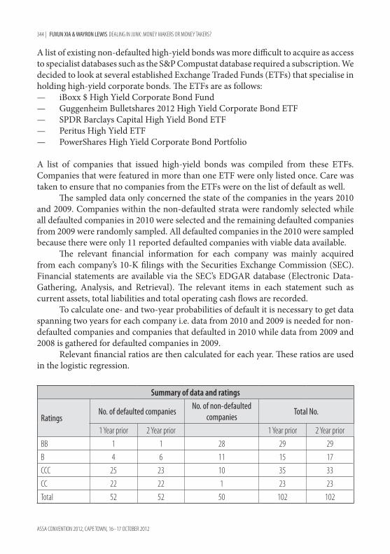
The sampled data only concerned the state of the companies in the years 2010 and 2009. Companies within the non-defaulted strata were randomly selected while all defaulted companies in 2010 were selected and the remaining defaulted companies from 2009 were randomly sampled. All defaulted companies in the 2010 were sampled because there were only 11 reported defaulted companies with viable data available.

The relevant financial information for each company was mainly acquired from each company’s 10-K filings with the Securities Exchange Commission (SEC). Financial statements are available via the SEC’s EDGAR database (Electronic Data-Gathering, Analysis, and Retrieval). The relevant items in each statement such as current assets, total liabilities and total operating cash flows are recorded.

To calculate one- and two-year probabilities of default it is necessary to get data spanning two years for each company i.e. data from 2010 and 2009 is needed for non-defaulted companies and companies that defaulted in 2010 while data from 2009 and 2008 is gathered for defaulted companies in 2009.

Relevant financial ratios are then calculated for each year. These ratios are used in the logistic regression.

Summary of data and ratings

RatingsNo. of defaulted companies

No. of non-defaulted companies

Total No.

1 Year prior 2 Year prior 1 Year prior 2 Year priorBB 1 1 28 29 29B 4 6 11 15 17CCC 25 23 10 35 33CC 22 22 1 23 23Total 52 52 50 102 102



6.1 Preliminary analysisAs seen from the sample above, 86.5% of defaulted bonds are at or below CCC rating at least two years before default. However there are 22% of non-defaulted bonds that are also CCC or below. There are only 9.6% of defaulted bonds with ratings of B and above while 78% of non-defaulted bonds are above B.

We can see from this that a better rating is a better indicator of a company not likely to default than a poor rating which does not indicate clearly if a company will default or not.

Looking at the general financial attributes of the sampled firms (see table below), we can see that the leveraged companies are all characterised by a high-debt ratio, low cash to assets and loss-making as seen from negative net incomes.

We can see that there is generally a significant difference in total assets of firms which have defaulted and firms which have not. It is clear that bigger companies are generally more secure than smaller firms. We can see that in terms of equity, companies, prior to experiencing default within less than two years, have significantly fewer surplus assets compared to companies that did not default. A company prior to default is exposed through its negative equity value, showing that as the company’s liabilities exceed the assets, default occurs rapidly as there is no way for the assets to cover the growing debt.

Earnings before interest and taxes (EBIT) also vary significantly between defaulted and non-defaulted firms. Defaulted firms generally have a lower EBIT and it can go into the negative. It may be thought that a company with a high EBIT can make its interest payments and thus not default even though they are making a loss. As can been seen from the second year data, defaulted and non-defaulted firms have a significant difference in EBIT but not in net income.

We can also see there is a big difference in operating cash flows between the two types of firms. Firms that do not default have significant cash flows coming in through their operations. It can be seen that a firm in distress is more likely to default if it has been selling its assets or refinancing its debt rather than earning cash through its operations. Note also that there is no significant difference in terms of total cash flows for the two types of firms.

Surprising results are seen when looking at the variables that were not significantly different between the two types of firms. Cash levels, current liability levels and total liability levels showed no distinctive trait differentiating between defaulted and non-defaulted. It is surprising as several common ratios are based upon those exact items such as current ratio, debt ratio etc. We shall examine the power of these traditional ratios in determining default in our analysis.

T-statistics which show a significant difference in means between defaulted and non-defaulted variables are highlighted in the table that follows.



Summary of Financial Positions of Sample Companies (in Millions)

Cash TA CL TL E EBIT NI CFO CF

1 Year prior

Mean

Defaulted 594 7675 2762 8284 –664 –429 –757 81 –211

Non-Defaulted 1050 17394 2595 13846 2831 1187 292 937 175

Standard Deviation

Defaulted 3050 31087 13850 33304 4684 1585 2369 304 175

Non-Defaulted 1551 12376 2697 15911 3098 1529 1741 1174 1356

T-Statistic 1.06 2.21 –0.09 1.18 9.39 3.9 3.13 19.76 1.56

2 Year Prior

Mean

Defaulted 800 9014 2970 8658 363 52 –312 499 146

Non-Defaulted 991 17307 2466 14116 2504 287 –431 999 68

Standard Deviation

Defaulted 4877 39206 17030 38713 2111 1313 1428 2366 770

Non-Defaulted 1627 20227 3616 18708 4678 2209 1594 1255 854

T-Statistic 0.28 1.5 –0.21 1 7.17 2.46 –0.59 1.5 –0.72

Key TA : Total Assets CL: Current Liabilities Tl: Total Liabilities EBIT: Earnings before interest and tax E: Total Shareholder’s Equity NI: Net income CFO: Operating Cashflows CF : Total Cashflows

The T-Statistic is calculated as follows: 1 2

1 2

X X 1 1

Ts

N N

−=

−

where ( ) 2 21 2 2

1 2

1 1 ( 1)

2N s N s

sN N

− + −=

+ −

X1 is the mean of the non-defaulted variable.X2 is the mean of the defaulted variable.S1 is the standard deviation of the non-defaulted variable.S2 is the standard deviation of the defaulted variable.S is the weighted average standard deviation of all samples.N1 is the number of non-defaulted samples.N2 is the number of defaulted samples.



7. METHODOLOGYWe used multivariate logistic regression analysis to estimate the probabilities of default for high-yield bond issuing companies. The general formula for the model is given by:

0ln 1

n

i ii

xϑ β βϑ

= + − ∑

where ϑ is the probability of default, the 'iβ s are the parameters and the xis are the covariates (financial ratios and variables).

Fifty-two ratios and variables were tested for data available one year prior to default and data available two years prior to default respectively. The ratios and variables are of the following types: credit rating, cash flows, liquidity, size, efficiency, profitability, and leverage. All variables employed in Huffman and Ward (1996) and Bryan, Marchesini and Perdue (2004) were used in our analysis, thereby including those used by Altman (1968) and Beaver (1966) as well. This was done so that the widest possible selection of covariates could be covered. Conventional financial ratios such as the current ratio, debt ratio, return on assets and return on equity were also included in order to gauge their significance.

It was decided to develop two models for each dataset: one including credit ratings and the other excluding credit ratings. We included credit ratings to determine if Hilscher and Wilson’s (2010) results were skewed due to their inclusion of investment grade ratings in their study. Additionally, although they determined that a credit rating is a poor indicator of a probability of default, they did not test if a credit rating in conjunction with other fundamental factors could improve a model of default.

The credit ratings were grouped to achieve an acceptable balance between homogeneity and credibility. For example, firms with ratings of CCC+ and CCC– were placed in the same rating group CCC.

Credit ratings were then excluded for the second model to examine how the likelihood of default is affected solely by the fundamental aspects of the companies instead of external factors such as ratings or the economy.

We followed a process similar to that of the purposeful selection of covariates (Bursac et al., 2008). Each covariate was tested individually to determine the significance of its influence on the probability of default. In order to obtain a multivariate model the resulting set of significant covariates was then tested simultaneously and consequent insignificant covariates were systematically removed. We employed a p-value cut-off point of 0.5 on the first run and decreased the cut-off point by 0.1 on each consequent run until a set remained where each covariate was ideally significant at the 5% level. The initial p-value cut-off point may seem too high but the more common smaller values 0.05 and 0.1 have failed previously in identifying covariates known to be significant (Bursac et al., 2008). Finally, the covariates that were removed were then added back one by one to identify any variables that contributed to the significance of the multivariate model. Interaction terms consisting of the covariates in the final



multivariate model were then also tested with the aim of improving the accuracy of the model’s predictions. A table containing all the financial ratios and variables which were tested can be found in the Appendix A.

8. RESULTSThe multivariate logistic regression analysis results in four models being obtained for predicting the likelihood of default: two models including credit ratings and two models excluding credit ratings. The models give the one-year and two-year default probabilities for companies based on information freely available in their financial statements at the time. The models and R-Square (the measure of the accuracy of the model in predicting future outcomes) are presented below.

8.1 Models including credit ratingsOne year prior to default:

Model 1: ln 1ϑϑ

= − 15.0025+2.0468Θ–51.9534BEPR–1.7463LNTA

+ 50.6348EBITDATA–3.3867Ψ–0.6452EBITINT

The R-Square is 67.39% 1 01 1if RATINGBBif RATINGBB

=− =

1 01 1

if RATINGCCif RATINGCC

= − =

Θ

Ψ

Two years prior to default:

Model 2: ln1ϑϑ

= − 13.9078+1.4690Θ–1.3327Ψ–1.6499LNTA

+ 1.1774STDEBTE

The R-Square is 59.32%.

8.2 Models excluding credit ratingsOne year prior to default:

Model 3: ln 1ϑϑ

= − 17.9995–22.0935BEPR–1.7696LNTA–0.9715LNTA_TETA

+5.4392CFOSALES–43.0116 CFOTA+3.1164RETA*

The R-Square is 64.68%

* The parameter for RETA is significant at the 10% level.



Two years prior to default:

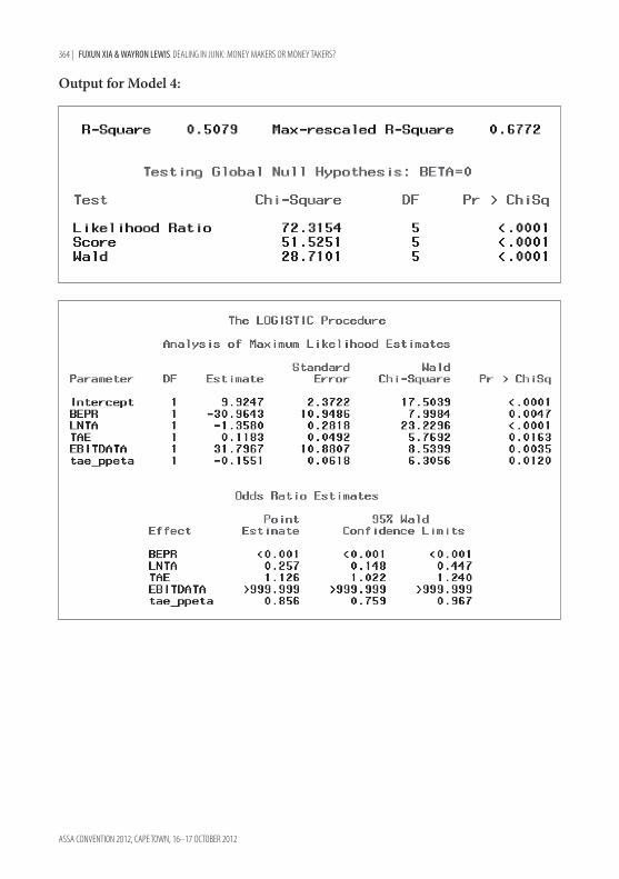
Model 4: ln1ϑϑ

= − 9.9247–30.9643BEPR–1.3580LNTA + 0.1183TAE +

31.7967EBITDATA–0.1551TAE_PPETA

The R-Square is 50.79%.

Explanation of the covariates in Model 1, Model 2, Model 3 and Model 4:

Ratio/Variable Formula DescriptionRATINGBB S&P rating in the BB categoryRATINGCC S&P rating in the CC categoryEBIT Earnings Before Interest & TaxEBITINT EBIT/Interest Expense TIE RatioBEPR EBIT/Total Assets Basic Earnings Power RatioSTDEBTE Short Term Debt/Shareholders’ EquityLNTA ln (Total Assets)CFOSALES Operating Cash Flows/RevenuesCFOTA Operating Cash Flows/Total AssetsRETA Retained Earnings/Total AssetsTAE Total Assets/Shareholders’ EquityEBITDA EBIT + Depreciation & Amortisation Earnings Before Interest, Tax, Depreciation &

AmortisationEBITDATA EBITDA/Total AssetsPPE Property, Plant & EquipmentPPETA PPE/Total AssetsTAE_PPETA TAE PPETATETA Total Equity/Total AssetsLNTA_TETA LNTA TETA

Naturally, the credit ratings were expected to be significant in determining default probabilities as confirmed by the logistic regression analysis. It is not surprising either that ratios including total assets such as BEPR, CFOTA, RETA, TAE and specifically LNTA (since it is a direct measure of the size of the total assets) are significant or that ratios including EBIT and operating cash flows (EBITDATA, EBITINT, CFOSALES and CFOTA are significant as well. The preliminary analysis carried out on the data revealed that the size of total assets, EBIT and operating cash flows differed considerably between defaulting and non-defaulting companies. It is worth noting, however, that



the more common accounting and gearing ratios such as the current ratio, debt ratio, TIE (Times Interest Earned), asset cover, ROA (Return On Assets) and ROE (Return On Equity) did not turn out to be significant in determining the likelihood of default by a particular company.

Figure 2 Nominal GDP Growth: The GDP growth is easily obtainable from any statistical source. We used the website www.measuringworth.com.

Figure 1 UMICS Index Value: The monthly UMICS data is retrieved from the index archive from the year 2000 onwards and is averaged to obtain an annual index value.



We also decided to assess the claims of Bryan, Marchesini and Perdue (2004), who stated that macro-economic factors could also affect a firm’s likelihood of default.

Due to our data being constrained to 2009 and 2010 we soon realised that we could not incorporate macro-economic factors into our models. Therefore we decided to undertake a simple linear regression analysis on aggregate default rates in the period 2000 to 2010 using a number of macro-economic factors in order to investigate if these factors would play a key role in determining whether high-yield bond issuers would default or not.

We decided to use nominal GDP growth, real GDP growth and the University of Michigan Index of Consumer Sentiment (UMICS) as indicators of the macro-economic conditions. We believe this is the first study that incorporates UMICS as a viable macro-economic factor.

The UMICS is released monthly by the University of Michigan and Thomson Reuters. The index is compiled through a national survey by carrying out telephone interviews. Representative households throughout the USA are contacted to find out their views on their own financial situation, the short-term general economy and the long-term general economy. This index is generally a very accurate representation of the state of the economy in the USA and has broad implications for the stock, bond and dollar market. A low relative value indicates a lower confidence in the US economy as a whole.

We obtained the aggregate default rates for speculative-grade debt issuers, nominal GDP growth, real GDP growth and the value of the UMICS over the period 2000 to 2010.

Figure 3 Real GDP Growth: The GDP growth is easily obtainable from any statistical source. We used the website www.measuringworth.com.



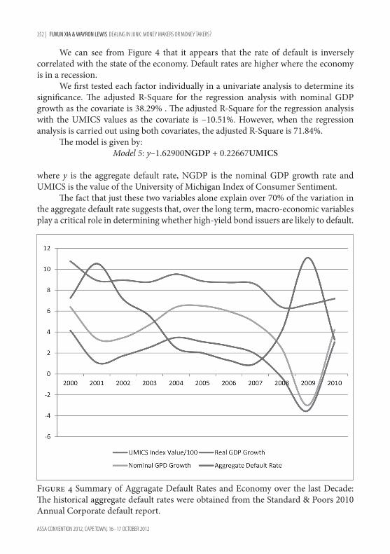
We can see from Figure 4 that it appears that the rate of default is inversely correlated with the state of the economy. Default rates are higher where the economy is in a recession.

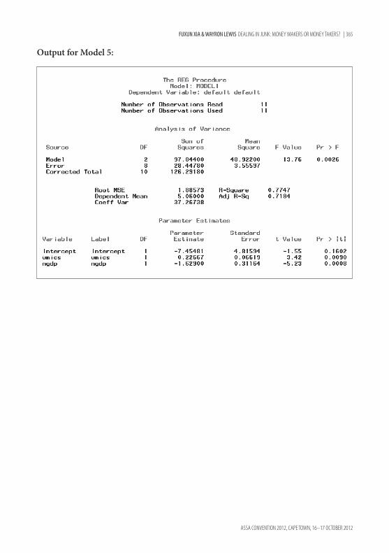
We first tested each factor individually in a univariate analysis to determine its significance. The adjusted R-Square for the regression analysis with nominal GDP growth as the covariate is 38.29% . The adjusted R-Square for the regression analysis with the UMICS values as the covariate is –10.51%. However, when the regression analysis is carried out using both covariates, the adjusted R-Square is 71.84%.

The model is given by: Model 5: y–1.62900NGDP + 0.22667UMICS

where y is the aggregate default rate, NGDP is the nominal GDP growth rate and UMICS is the value of the University of Michigan Index of Consumer Sentiment.

The fact that just these two variables alone explain over 70% of the variation in the aggregate default rate suggests that, over the long term, macro-economic variables play a critical role in determining whether high-yield bond issuers are likely to default.

Figure 4 Summary of Aggragate Default Rates and Economy over the last Decade: The historical aggregate default rates were obtained from the Standard & Poors 2010 Annual Corporate default report.



This also suggests that, if the data were readily available, a comprehensive modelling exercise incorporating these variables together with financial ratios and variables has the potential to result in a powerful tool capable of aiding investors in making important investment decisions in the high-yield debt market.

Due to this finding we decided to collect additional data to form a small dataset. We obtained information for 33 companies relating to the period 2000 to 2010. We included nominal GDP growth and the UMICS values in our dataset and proceeded to obtain a model as described for models 1 to 4. A viable multivariate model with significant covariates could not be obtained when financial ratios and the macro-economic factors were used in conjunction; however, nominal GDP growth was significant in isolation. We attribute this partly to the fact that financial ratios and variables could possibly not be as good indicators of the likelihood of default over the long term as macro-economic factors seem to be, and partly to the sample error inherent in our data. See Appendix B for the results.

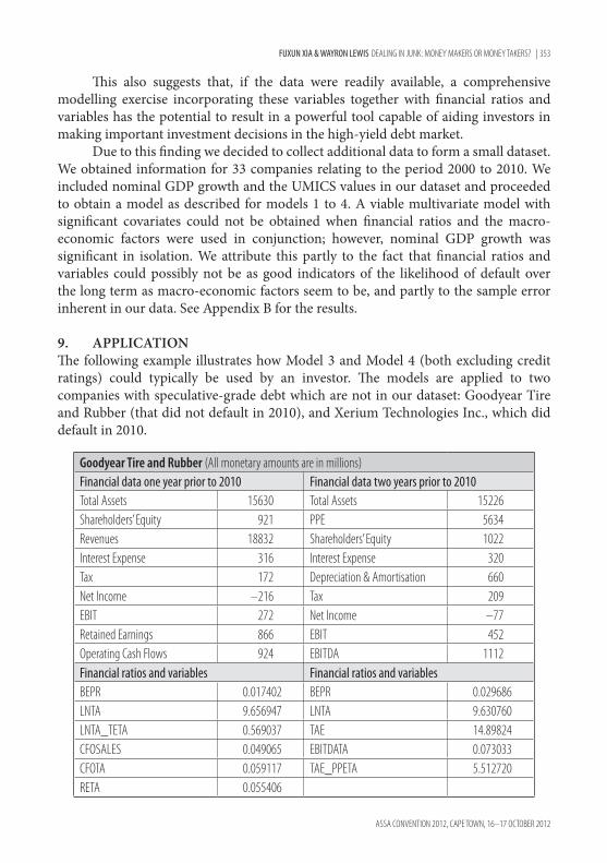
9. APPLICATIONThe following example illustrates how Model 3 and Model 4 (both excluding credit ratings) could typically be used by an investor. The models are applied to two companies with speculative-grade debt which are not in our dataset: Goodyear Tire and Rubber (that did not default in 2010), and Xerium Technologies Inc., which did default in 2010.

Goodyear Tire and Rubber (All monetary amounts are in millions)Financial data one year prior to 2010 Financial data two years prior to 2010Total Assets 15630 Total Assets 15226Shareholders’ Equity 921 PPE 5634Revenues 18832 Shareholders’ Equity 1022Interest Expense 316 Interest Expense 320Tax 172 Depreciation & Amortisation 660Net Income –216 Tax 209EBIT 272 Net Income –77Retained Earnings 866 EBIT 452Operating Cash Flows 924 EBITDA 1112Financial ratios and variables Financial ratios and variablesBEPR 0.017402 BEPR 0.029686LNTA 9.656947 LNTA 9.630760LNTA_TETA 0.569037 TAE 14.89824CFOSALES 0.049065 EBITDATA 0.073033CFOTA 0.059117 TAE_PPETA 5.512720RETA 0.055406



Applying Model 3 gives a probability of default of 0.082504 (8.25%) in 2010 given information in 2009 and applying Model 4 gives a probability of default of 0.300812 (30.08%) in 2010 given information in 2008.

Xerium Technologies Inc. (All monetary amounts are in millions)Financial data one year prior to 2010 Financial data two years prior to 2010Total Assets 693.5 Total Assets 818.1Shareholders’ Equity –119.7 PPE 384.6Revenues 500.1 Shareholders’ Equity –27.6Interest Expense 68.5 Interest Expense 60.3Tax 12.3 Depreciation & Amortisation 46Net Income –112 Tax 3.9EBIT –31.2 Net Income 26.6Retained Earnings –330.9 EBIT 90.8Operating Cash Flows 16.1 EBITDA 136.8Financial ratios and variables Financial ratios and variablesBEPR –0.044989 BEPR 0.110989LNTA 6.541751 LNTA 6.706985LNTA_TETA –1.129124 TAE –29.641304CFOSALES 0.032194 EBITDATA 0.167217CFOTA 0.023216 TAE_PPETA –13.934783RETA –0.477145

Applying Model 3 gives a probability of default of 0.997671 (99.77%)in 2010 given information in 2009 and applying Model 4 gives a probability of default of 0.794388 (79.44%) in 2010 given information in 2008.

It seems logical that an investor faced with the choice of investing in either Xerium’s or Goodyear’s bonds in either 2008 or 2009 would opt for Goodyear if the results of the models were taken into consideration as part of the investment decision. It is then evident how the models could aid investors in choosing bond portfolios which are more suited to their respective risk appetites and desire for diversification within the fixed-interest asset class.

10. SOUTH AFRICAN COMPANIESThe South African high-yield debt market is still in its infancy. Mcnee (2006) points out South African companies are more likely to raise capital through bank loans than to tap the capital markets due to the repercussions on the economy caused by the apartheid era. Garth Greubel, CEO of the Bond Exchange of South Africa at the time,



also mentioned that bank lending as the major form of raising funds for corporates is very competitive and out-performs the relatively new corporate bond market which has only been around since 1998. According to a local banker, the South African corporate bond market is small and illiquid leading to small and illiquid bond derivative markets (Mcnee, 2006). Greubel also explained that investors in the domestic market would not be able to get diversification from the first high-yield issue by investing in similarly rated financial instruments. The small size of the high-yield debt market in South Africa can also be attributed to asset managers being unwilling to take on credit risk for the return on offer (Mcnee, 2006). The first two (off-shore) high-yield issues by South African companies were by Cell C and FoodCorp in 2005 (Mcnee, 2006). We only know of five or six issuers of domestic high-yield bonds in South Africa and therefore we expect that they are unlikely to be traded and would rather be held to maturity. We managed to acquire some data through the Johannesburg Stock Exchange concerning the junk bond issues and proceeded to undertake a small investigation into the characteristics of the issues.

High-yield bond issues data (as at 29 July 2011).

Issuer Rating Issue amount Coupon GRY Maturity date

Blue Granite Investments (Pty) Ltd Ba2 106 000 000.00 8.825 9.86 21 March 2037

Blue Granite Investments (Pty) Ltd B2 32 000 000.00 12.825 13.42 21 March 2037

Blue Granite Investments (Pty) Ltd Ba2 45 000 000.00 9.575 9.9 21 November 2032

Blue Granite Investments (Pty) Ltd Ba2 62 000 000.00 8.825 6.87 30 October 2031

Blue Granite Investments (Pty) Ltd Ba2 12 400 000.00 12.825 13.92 30 October 2031

Kagiso Sizanani Capital (Pty) Ltd Ba2 8 000 000.00 8.775 13.86 01 February 2012

Private Commercial Mortgages (Pty) Ltd Ba3 22 000 000.00 10.075 10.45 20 December 2025

Private Residential Mortgages (Pty) Ltd Ba2 34 000 000.00 7.775 8 15 June 2036

Private Residential Mortgages (Pty) Ltd Ba3 62 200 000.00 8.575 8.85 15 December 2035

We can see that all the issues are rated just below investment grade leading us to believe that they are fallen angels and hence are not purely junk bond issues. Eight out of the nine issues above have higher gross redemption yields than coupon rates, indicating that the bonds would currently trade at a discount which is indicative of the uncertain default risk associated with investing in junk bonds. The yields are higher than conventional government bonds but there are too few different issuers available to construct a satisfactorily diversified bond portfolio consisting only of South African junk bonds.



11. CONCLUSIONAlthough Hilscher and Wilson (2010) determined credit ratings to be a poor sole predictor of default, we find that when used in conjunction with other fundamental factors of a company issuing junk bonds, the credit ratings serve as powerful enhancements to a predictive model. It appears that certain ratings (BB, CC) will decrease or increase the likelihood of default should a company possess those ratings at least two years before a critical time of investigation.

When examining Beaver’s (1966) claim of window dressing commonly looked-at ratios, we found that the current ratios, debt ratios, return on assets and return on equity did not have high predictive powers in our multivariate models as mentioned above. When examined in isolation, we found that some degree of window dressing was present, with barely any difference in the average current ratios and return on assets between defaulted and non-defaulted companies. However there is a significant difference in the average debt ratios and return on equity. See Appendix C.

We believe that the gearing ratios are very useful in indicating if a company will issue junk or not, however they are not so prophetic as to further indicate if that company will default on their issue. We feel that is the reason why the ratios are not present in any of our developed models.

Although the more traditional accounting ratios did not provide significant information in modelling default of companies with high-yield bonds, we found ratios and variables incorporating the size of assets, EBIT (Earnings Before Interest & Tax) and operating cash flows to be key in developing the models for predicting default one and two years prior to default respectively.

Caution must be exercised when using our ratios to model default. Although investors can use our models to determine and price the risk of default of high-yield bonds, they should only do so in the short term as the significance of the ratios in modelling default reduces as the term increases. Long-term effects of macro-economic factors skew the results.

We found that macro-economic factors have potentially the greatest significance in predicting default for companies over the long term. It was shown that, when used in conjunction with each other, some macro-economic factors such as the University of Michigan Index of Consumer Sentiment (derived from a somewhat subjective source which we feel is the reason why it has not been previously used) prove to be surprisingly relevant and useful. Our new discovery of relevant subjective indices leads us to suggest that future in-depth research can be undertaken on the correlation between consumer indices and default rates.

Given a year’s nominal GDP growth and University of Michigan Index of Con-sumer Sentiment, it is possible to derive a baseline probability of default of high-yield corporate bonds with high accuracy. A prospective investor can utilise that value to determine possible diversification benefits and risks through investing in junk bonds.

Use of our models which are derived using US data in the South African context must be taken with a grain of salt, especially when the South African market is new



to the junk bond phenomenon. There is huge potential for growth and extraordinary profits as the market in South African booms in the future. Being a late bloomer, we believe that the South African market will avoid the growing pains associated with the US junk bond market as evidenced in the 1980s and 1990s. Thus, our models could remain relevant in the context of South Africa.

Lastly, due to the intensive and time-consuming method of our data collection, despite gathering enough data for the result to be statistically significant, we are curious about possible improvements to the R-square of the models, had a larger sample been collected. It is our recommendation that further studies concerning the significance of macro-economic factors vs. fundamental characteristics on default rates be undertaken as the primary focus. Our results on ratios vs. macro-economic factors are possibly skewed in light of our sample consisting of 33 firms used during the analysis.

ACKNOWLEDGEMENTSWe would like to express our gratitude to the following people for their generosity, time, insights and contributions to our study: Nicky Newton-King of the JSE; Prof. Eben Mare of Stanlib; Rajith Sebastian of Standard Chartered Bank; Byran Taljaard of JM Busha Investments; Dr Conrad Beyers of University of Pretoria; and Michelle Reyers of University of Pretoria

REFERENCESAltman, EI (1968). Financial ratios, Discriminant Analysis and the Prediction of Corporate

Bankruptcy. Journal of Finance, 23(4), 569–89.Asquith, P, Gertner, R and Scharfstein, D (1994). Anatomy of distress: An examination of junk-

bond issuers. Quarterly Journal of Economics, 109(3), 625–58Beaver, WH (1966). Alternative Financial Ratios as Predictors of Failure. Journal of Accounting

Research. Supplement, Accounting Review, 71–111.Bohn, J and Crosbie, P (2003). Modeling Default Risk, Mood’s KMV Company. Viewed 7 April

2011, <http://business.illinois.edu/gpennacc/MoodysKMV.pdf>.Bryan, V, Marchesini, R and Perdue, G (2004). Applying Bankruptcy Prediction Models to

Distressed High Yield Bond Issues. Journal of Fixed Income, 13(4), 50–6.Bursac, Z, Gauss, CH, Hosmer, DW and Williams, DK (2008). Purposeful selection of variables

in logistic regression. Source Code for Biology and Medicine, viewed 20 September 2011, www.scfbm.org/content/pdf/1751-0473-3-17.pdf

Hakim, SR and Shimko, D (1995). The Impact of firms’ characteristics on junk-bond default. Journal of Financial and Strategic Decisions, 8(2), 47–55.

Helgewe, J and Kleiman, P (1996). Understanding Aggregate Default Rates of High Yield Bonds. Current Issues in Economics and Finance, 2(6), 1–6.



Hilscher, J and Wilson, M (2010). Credit ratings and credit risk. Brandeis University, Department of Economics and International Business School, Working Papers. no. 31.

Huffman, SP and Ward, DJ (1996). The Prediction of Default for High Yield Bond Issues. Review of Financial Economics, 5(1), 75–89.

Lewis, M (1989). Liar’s Poker. pp. 245–65. Great Britain: Hodder and Stoughton.McDonald, CG and Van de Gucht, LM (1999). High-yield bond default and call risks. The

Review of Economics and Statistics, 81(3), 409–19.Mcnee, A (2006). South Africa new beginnings. Risk.net Financial risk Management News and

Analysis. Viewed 7 October 2011, www.risk.net/credit/feature/1522836/south-africa-new-beginnings

Merton, RC (1974). On the pricing of corporate debt: The risk structure of interest rates. Journal of Finance. 29(2), 449–70.

Micocci, M (2000). M.A.R.C.: An actuarial model for credit risk. ASTIN Colloquium International Actuarial Association – Brussels, Belgium. Viewed 7 October, 2011. www.actuaries.org/ASTIN/Colloquia/Porto_Cervo/Micocci.pdf

Mirkin, V (2009). Credit Risk and Liquidity: Markets, Methods and Modelling Strategies. Staple Inn Actuarial Society.

NYU Salomon Center, Stern School of Business (October 2006). “Default, Recovery Rates Defy Forecasts in High Yield, Distressed Debt Markets” Turnaround Management Association. Viewed 7 April, www.data360.org/dsg.aspx?Data_Set_Group_Id=1369

Sakoui, A (January 10, 2010). “Europe braced for boom in junk bonds”, Financial Times.Sweeting, P (2002). The Role of High Yield Corporate Debt in Pension Schemes. Paper presented

to the Staple Inn Actuarial Society, 7 May 2002.Theunissen, G (November 16, 2010). “South Africa’s High-Yield Bond Market to Jump Tenfold,

Investec Says”, Bloomberg.Yago, G (n.d.). Junk Bonds. The Concise Encyclopaedia of Economics, viewed 7 April 2011,

www.econlib.org/library/Enc/JunkBonds.html.



APPENDIX A

Financial ratios and variables tested in the logistic regression analysis.

Ratio/Variable Formula DescriptionRATINGB S&P rating is in B categoryRATINGBB S&P rating is in BB categoryRATINGCC S&P rating is in CC categoryCR Current Assets/Current Liabilities Current RatioWCTA Working Capital/Total AssetsRETA Retained Earnings/Total Assets

EBIT Earnings Before Interest & TaxBEPR EBIT/Total Assets Basic Earnings Power RatioED Equity/Total DebtSALESTA Revenue/Total AssetsLEVERAGE Long Term Debt/Total AssetsNDB Long Term Debt + Short Term Debt – Cash Net Debt BorrowedNDR NDB/(Shareholders’ Equity + NDB) Net Debt RatioNWC (Current Assets–Current Liabilities)/Total AssetsCHGNWC NWCt–NWCt–1

EBITS EBIT/RevenuesPPE Property, Plant & EquipmentPPETA PPE/Total AssetsTANGTA (Total Assets – Intangibles)/Total AssetsTMV Shareholders’ Equity + Total Debt Total Market Value of AssetsFCF Operating Income – Interest Expense – Income Tax –

DividendsFree Cash Flow

FCFTMV FCF/TMVLNTA ln(Total Assets)TETA Total Equity/Total AssetsEBITDA EBIT + Depreciation & AmortisationEBITDASALES EBITDA/RevenueAC {(Total Assets–Intangibles)–(Current Liabilities

Short-term Debt Obligations)}/Total Debt OutstandingAsset Coverage Ratio

NISALES Net Income/RevenuesROA Net Income/Total Assets Return On Assets



ROE Net Income/Shareholders’ Equity Return On EquityTAE Total Assets/Shareholders’ EquityCASHSALES Cash/RevenueDEBTRATIO Total Debt/Total Assets Debt RatioSTDEBTE Short-term Debt/Shareholders’ EquityCFODEBT Operating Cash Flows/Total DebtCFOSALES Operating Cash Flows/RevenuesCFOE Operating Cash Flows/Shareholders’ EquityCFOINT Operating Cash Flows/Interest ExpenseCFOTA Operating Cash Flows/Total AssetsEBITINT EBIT/Interest ExpenseCFO_INT_TMV (Operating Cash Flows + Interest Expense)/TMVCINDEBT Investing Cash Flows/Total DebtCINSALES Investing Cash Flows/RevenuesCINE Investing Cash Flows/Shareholders’ EquityCININT Investing Cash Flows/Interest ExpenseCINTA Investing Cash Flows/Total AssetsCFINDEBT Financing Cash Flows/Total DebtCFINSALES Financing Cash Flows/RevenuesCFINE Financing Cash Flows/Shareholders’ EquityCFININT Financing Cash Flows/Interest ExpenseCFINTA Financing Cash Flows/Total AssetsCFDEBT Total Cash Flows/Total DebtCFSALES Total Cash Flows/RevenuesCFE Total Cash Flows/Shareholders’ EquityCFINT Total Cash Flows/Interest ExpenseCFTA Total Cash Flows/Total AssetsLNTA_TETA LNTA×TETATAE_PPETA TAE×PPETA



Output for Model 1:



Output for Model 2:



Output for Model 3:



Output for Model 4:



Output for Model 5:



APPENDIX B

All the parameters are insignificant as can be seen from the SAS output above.



APPENDIX C

Average of traditional ratios for defaulted & non-defaulted firms

Current ratio Debt ratioReturn on

AssetsReturn on

EquityAsset Cover

Defaulted 1.52 0.94 –0.21 2.55 1.22

Non-defaulted 1.56 0.53 0.02 0.13 1.51

dealing in junk: money makers or money takers? · fuxun xia & wayron lewis dealing in junk:...

Documents