death and its determinants - cass business school · death and its determinants longevity and...

Death and its DeterminantsLongevity and Capital Market Solutions Conference

Frankfurt 8-9 September 2011

Declan French (CoE NI) and

Colin O’Hare (QUMS NI)

Outline of presentation

• Motivation and context within modeling mortality

• Review of existing Stochastic atheoretical models

• Data sources and quality

• The methodology

• The fitting and forecasting results

• Annuity pricing implications

• Conclusions from the results and further research

Motivation and context within modeling mortality

• Longevity risk a significant risk to be managed

• Significant literature identifying and modeling the improvement in mortality

• Stochastic “extrapolative” models well established

• Lee Carter (1992), Brouhns et al (2002), Renshaw and Haberman (2003,2006) , Cairns et al (2006,2009), Currie (2006), Girosi and King (2005),….

• Common trends identified and forecast

Motivation continued

• Incorporating observable factors that may explain trends is missing from the literature

• atheoretical models identified evidence for and added factors to improve the fit

• Little attention is paid to the forecasting ability

• Little attention is paid to a rigorous approach to identifying the necessary number of parameters





• The methodology




Review of existing Stochastic atheoretical models

• Lee Carter identified a single time trend in mortality rates

• Additional trend in cohort identified in Renshaw & Haberman (2003,2006) and Currie (2006)

• Cairns (2006) linked the second trend to time and developed a series of models with two time trends and cohort effects

• Plat (2009) combined all trends with 4 factors (3 time related, 1 cohort)

( ), expx t x x t tm α β κ ε= + +

( )1 1 2, expx t x x t x t x tm α β κ β γ ε−= + + + ( )1

, expx t x t t x tm α κ γ ε−= + + +

( ) ( )1 2,logit( ) log 1x t x x t t tq q q x xκ κ ε= − = + − +

( ) ( )( )1 2 3, expx t x t t t t x tm x x x xα κ κ κ γ ε+

−= + + − + − + +

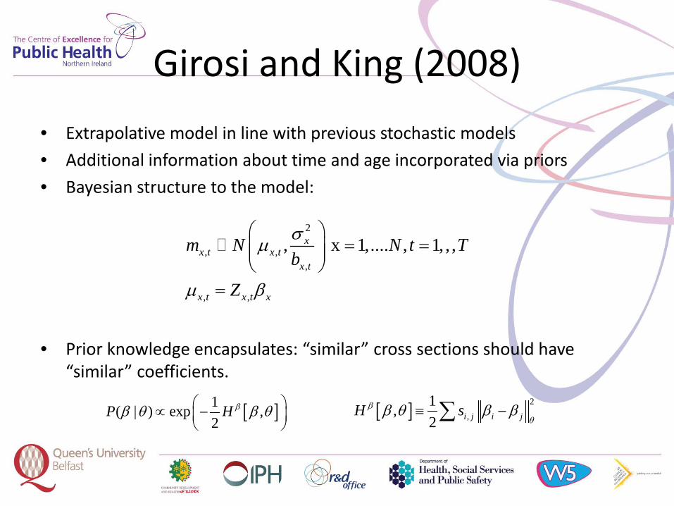
Girosi and King (2008)

• Extrapolative model in line with previous stochastic models

• Additional information about time and age incorporated via priors

• Bayesian structure to the model:

• Prior knowledge encapsulates: “similar” cross sections should have “similar” coefficients.

2

, ,,

, ,

, x 1,.... , 1, , ,xx t x t

x t

x t x t x

m N N t Tb

Z

σµ

µ β

= =

=

[ ]1( | ) exp ,2

P H ββ θ β θ ∝ −

[ ] 2

,1,2 i j i jH sβ

θβ θ β β≡ −∑

King and Soneji (2011)

• Inclusion of exogenous variables in addition to time trends

• Exogenous variables (smoking prevalence) lagged by 25 years taken from the literature

• They conclude that including risk factors (obesity and smoking) improves forecasts and shows mortality rate decline to be greater than that previously predicted.

• R package called “YourCast” used to applied this model

• Implemented in R and available from: http://gking.harvard.edu/yourcast

http://gking.harvard.edu/yourcast�





• The methodology




Data

• Mortality data taken from the Human Mortality database http://www.mortality.org

• Data on possible determinants of health taken from OECD health data 2009 http://www.oecd.org

• Study includes U.S., U.K. and Japan – Common characteristic: all with developed healthcare systems, all non-tropical

countries

– Differing characteristic: culture, diet and the significance of private vs public health expenditure

• Data taken from 1970 – 2000 and forecast from 2001-2006 inclusive and back testing carried out.

• Exogenous variables chosen included: Alcohol consumption, Tobacco consumption, GDP, Health expenditure, total fat intake, total fruit and vegetable consumption.

http://www.mortality.org/�

http://www.oecd.org/�

Data – Mortality rates

• Log mortality rates for the U.K., U.S. and Japan.

• Declining mortality rates

• Cohort effect visible

1950 1960 1970 1980 1990 2000 201010

-4

10-3

10-2

10-1

100

Year

UK

mal

e de

ath

rate

s by

sin

gle

age

,,

,

ln x tx t

x t

Dm

E

=

1950 1960 1970 1980 1990 2000 201010

-3

10-2

10-1

100

Year

US

mal

e de

ath

rate

s by

sin

gle

age

1950 1960 1970 1980 1990 2000 201010

-4

10-3

10-2

10-1

100

Year

Japa

n m

ale

deat

h ra

tes

by s

ingl

e ag

e

Data – exogenous variables

Alcohol Tobacco GDP

Fat Intake Health Expenditure Fruit and Veg intake

Data – exogenous variablesJ Mean Standard

DeviationDefinition

Alcohol (UK) 9.3 (US) 9.5

(Japan) 7.8

0.60.81.0

Annual consumption of pure alcohol in litres, per person, aged 15 years and over

Tobacco 234926453227

516667147

Annual consumption of tobacco items (eg cigarettes, cigars) in grams per person aged 15 years and over

Fat 138.9133.5

73.1

3.010.0

8.9

Total fat (grams per capita per day)

Fruit & Veg 151.8219.7173.1

14.317.6

8.8

All fruit and vegetable consumption (except wine) in kilos per capita

GDP 1189625420

2,994,819

22754712

707,685

Gross domestic product per capita in national currency units at 2000 price levels

Health exp 7122787

191,957

2221098

63,732

Total health expenditure (private and public) per capita in national currency units at 2000 price levels





• The methodology




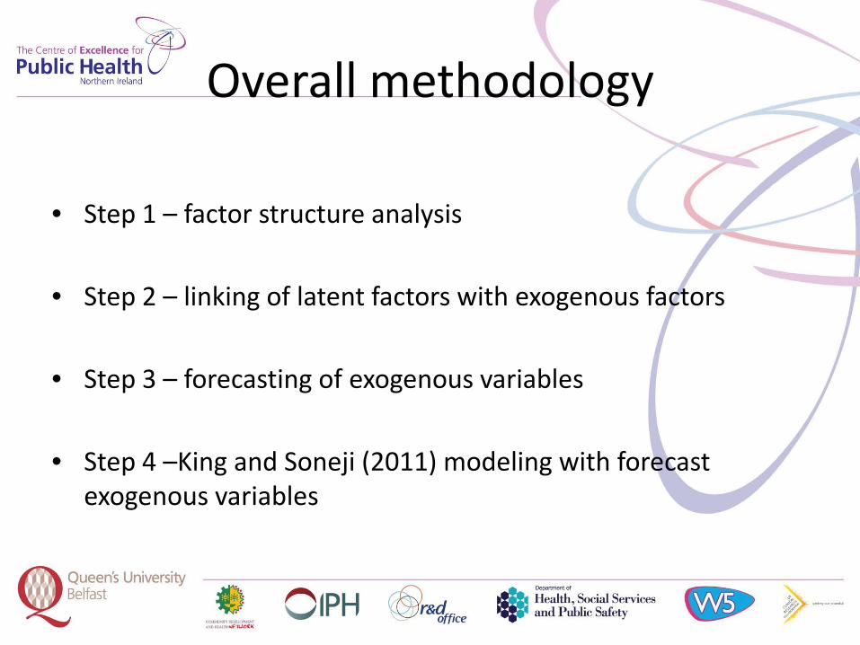
Overall methodology

• Step 1 – factor structure analysis

• Step 2 – linking of latent factors with exogenous factors

• Step 3 – forecasting of exogenous variables

• Step 4 –King and Soneji (2011) modeling with forecast exogenous variables

Factor structure analysis

• Principal components method applied

• Stopping rule applied to limit the number of extracted factors

• Method of Bai and Ng (2002) applied to determine the number of factors

• Information criterion used to limit factor extraction

• The number of factors “r” which minimises this gives the estimated number of factors.

Factor structure analysis

• Describe the N variables with a smaller number of factors F = (F1,…,Fr)

Data xit=λiF+eit i=1,...,N, t=1,...,T

• Using PC, factor estimates are given by the first r eigenvectors of the matrix XX’/(NT)

• Information criterion used to limit factor extraction

• The number of factors “r” which minimises this gives the estimated number of factors.

2 2

1 1

1( ) log ( ) ln[min( , )] where ( )N T

p iti t

N TIC r r r N T r eNT NT = =

+= ∂ + ∂ = ∑∑

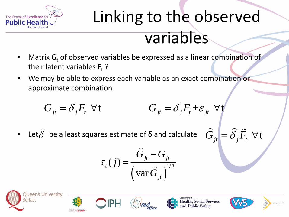
Linking to the observed variables

• Matrix Gt of observed variables be expressed as a linear combination of the r latent variables Ft ?

• We may be able to express each variable as an exact combination or approximate combination

• Let be a least squares estimate of δ and calculateδ

' tjt j tG Fδ= ∀ ' + tjt j t jtG Fδ ε= ∀

' tjt j tG Fδ= ∀

( )1/2( )var

jt jtt

jt

G Gj

Gτ

−=

Linking – Exact case

• Test the exogenous variables individually or as a group

• Test of individual exogenous variable consists of test statistic

(1) a test of the proportion of the time series for which the linear combination estimate deviates from the exogenous variable

(2) a test of how far the estimate is from the exogenous variabel over the whole time series

1

1( ) 1( ( ) )T

tA j jT ατ φ= >∑

1( ) ( )t T tM j Max jτ≤ ≤=

Linking – approximate case

• In the approximate case we are saying that there is some noise in the linear relationship between the exogenous variable and the latent factors.

• The two equivalent tests in this case are the noise to signal ratio and the coefficient of determination.

• In testing the group of exogenous variables we first look for the largest canonical relationship between linear combinations of exogenous variables. We then repeat the process but looking for a second relationship uncorrelated to the first etc.

var( ( ))( )var( ( ))

jNS jG jε

= 2 var( ( ))( )

var( ( ))G jR jG j

=

Linking – Canonical Correlations

• Testing the group as a set, the canonical correlations between G and F are considered.

• The first canonical correlation, ρ1, is the largest correlation that can be found for linear combinations of G and F.

• The second canonical correlation, ρ2, is the largest correlation that can be found from linear combinations of G and F uncorrelated with those giving the first canonical correlation, and so on.

• If all the m variables in are exact factors then the canonical correlations will all be unity. If the m variables are linearly dependent then the number of non-zero canonical correlations will be less than m.

Forecasting exogenous determinants

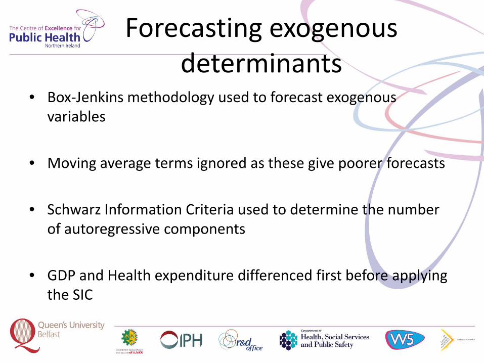
• Box-Jenkins methodology used to forecast exogenous variables

• Moving average terms ignored as these give poorer forecasts

• Schwarz Information Criteria used to determine the number of autoregressive components

• GDP and Health expenditure differenced first before applying the SIC

King and Soneji (2011) –The Model

• The King and Soneji model will include the exogenous variables selected

• Exogenous variables built into the model through the covariate beta vector, for example:

2

, ,,

, ,

, x 1,.... , 1, , ,xx t x t

x t

x t x t x

m N N t Tb

Z

σµ

µ β

= =

=

( )0 1, ,...gdp alc

x t x x t x x x tm year gdp alcβ β β β ε= + + + + +





• The methodology




Latent factor structure

• Using the methods of Bai and Ng (2002) with appropriate stopping rules we find the number of factors necessary to explain the data is:

– 2 factors explains 86% of variability for U.K.

– 4 factors explains 98% of the variability for U.S.

– 4 factors explains 98% of the variability for Japan

Latent factor structure

U.K. (2 factors) – factor 2 explaining the younger ages, factor 1 explaining the older ages

Latent factor structure• U.S. (4 factors) - Factors 1 and 4 explaining older ages, factors 2 and 3

explaining younger ages

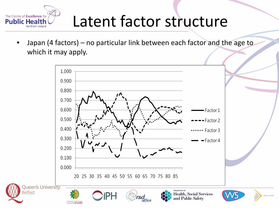
Latent factor structure• Japan (4 factors) – no particular link between each factor and the age to

which it may apply.

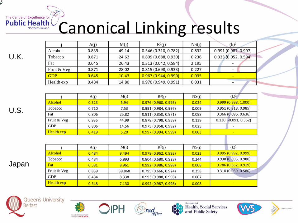
Canonical Linking resultsj A(j) M(j) R2(j) NS(j) (k)2

Alcohol 0.839 49.14 0.546 (0.310, 0.782) 0.832 0.991 (0.987, 0.997)Tobacco 0.871 24.62 0.809 (0.688, 0.930) 0.236 0.323 (0.052, 0.594)Fat 0.645 26.43 0.313 (0.042, 0.584) 2.195 -Fruit & Veg 0.871 28.02 0.815 (0.698, 0.933) 0.227 -GDP 0.645 10.43 0.967 (0.944, 0.990) 0.035 -Health exp 0.484 14.80 0.970 (0.949, 0.991) 0.031 -

j A(j) M(j) R2(j) NS(j) (k)2

Alcohol 0.323 5.94 0.976 (0.960, 0.993) 0.024 0.999 (0.998, 1.000)

Tobacco 0.710 7.53 0.991 (0.984, 0.997) 0.009 0.951 (0.918, 0.985)

Fat 0.806 25.82 0.911 (0.850, 0.971) 0.098 0.366 (0.096, 0.636)

Fruit & Veg 0.935 44.99 0.878 (0.798, 0.959) 0.139 0.130 (-0.091, 0.352)

GDP 0.806 14.56 0.975 (0.958, 0.992) 0.025 -Health exp 0.419 5.20 0.997 (0.994, 0.999) 0.003 -

j A(j) M(j) R2(j) NS(j) (k)2

Alcohol 0.484 9.494 0.978 (0.962, 0.993) 0.023 0.995 (0.992, 0.999)

Tobacco 0.484 6.893 0.804 (0.680, 0.928) 0.244 0.938 (0.895, 0.980)

Fat 0.581 8.961 0.992 (0.986, 0.998) 0.008 0.786 (0.652, 0.919)

Fruit & Veg 0.839 39.868 0.795 (0.666, 0.924) 0.258 0.310 (0.039, 0.580)

GDP 0.484 8.338 0.993 (0.988, 0.998) 0.007 -Health exp 0.548 7.130 0.992 (0.987, 0.998) 0.008 -

U.K.

U.S.

Japan

ARIMA Modeling of exogenous variables

No allowance for Moving Average terms in the ARIMA forecast

Used SIC to test for various Autoregressive terms

U.K.

GDP – ARIMA(2,1,0)

U.S.

Health – ARIMA(1,1,0)

Alcohol – ARIMA(3,0,0)

Japan.

Health – ARIMA(0,1,0)

Fat Intake – ARIMA(1,0,0)

Alcohol – ARIMA(1,0,0)

Measures of quality

• The average error E1 – this equals the average of the standardized errors, i.e. Errorx/n, where n = the number of ages included in the summation, that is the mean of the differences. This is a measure of the overall bias in the projections.

• The average absolute error E2 – this equals the average of |Errorx|, that is the mean of the absolute differences. This is a measure of the magnitude of the differences between the actual and projected rates.

• The standard deviation of the error E3 – this equals the square root of the average of the squared errors (Errorx

2), the root mean squares of the differences between the projected and actual rates.

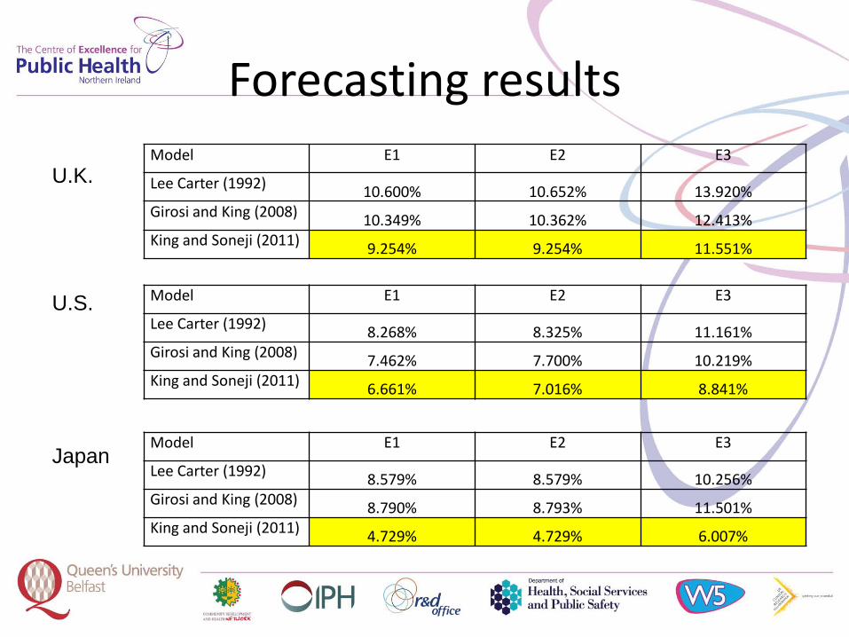
Forecasting resultsModel E1 E2 E3

Lee Carter (1992) 10.600% 10.652% 13.920%Girosi and King (2008) 10.349% 10.362% 12.413%King and Soneji (2011) 9.254% 9.254% 11.551%

Model E1 E2 E3


Model E1 E2 E3


U.K.

U.S.

Japan

Fitting resultsModel E1 E2 E3


Model E1 E2 E3

Lee Carter (1992) 0.333% 3.832% 5.784%Girosi and King (2008) 0.040% 4.119% 5.986%King and Soneji (2011) -0.089% 2.551% 3.402%

Model E1 E2 E3


U.K.

U.S.

Japan

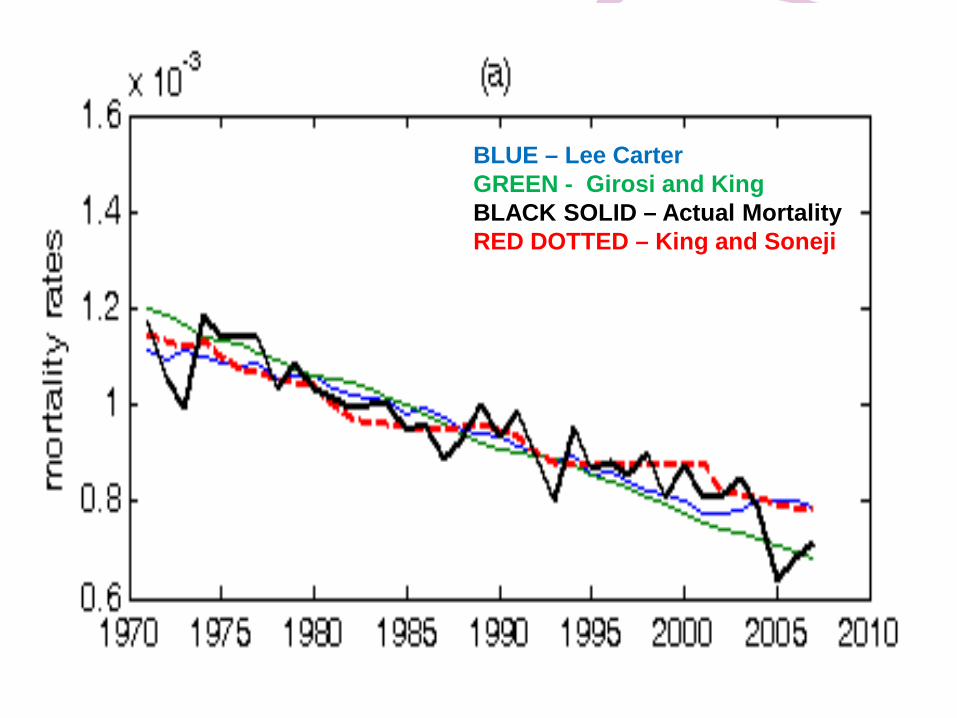
BLUE – Lee CarterGREEN - Girosi and KingBLACK SOLID – Actual MortalityRED DOTTED – King and Soneji

U.K. results

Figure 14 U.K. mortality rates fitted between 1970–2000, and forecast from 2001 - 2006 for the Lee Carter,(blue), Girosi and King (green), King and Soneji, (bold red dashed) models and actual mortality rates 1970-2006 (bold black) for males aged (a) 20, (b) 40, (c) 60 and (d) 80

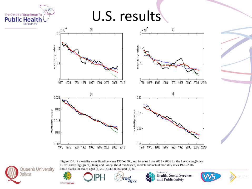
U.S. results

Figure 15 U.S mortality rates fitted between 1970–2000, and forecast from 2001 - 2006 for the Lee Carter,(blue), Girosi and King (green), King and Soneji, (bold red dashed) models and actual mortality rates 1970-2006 (bold black) for males aged (a) 20, (b) 40, (c) 60 and (d) 80

Japan results

Figure 16 Japan mortality rates fitted between 1970–2000, and forecast from 2001 - 2006 for the Lee Carter,(blue), Girosi and King (green), King and Soneji, (bold red dashed) models and actual mortality rates 1970-2006 (bold black) for males aged (a) 20, (b) 40, (c) 60 and (d) 80





• The methodology




Annuity pricing implications – U.K.

• King and Soneji(2011) vs Lee Carter(1992)

Annuity pricing implications – U.S.


Annuity pricing implications – Japan






• The methodology




Conclusions from the results

• Our model forecasts better than atheoretical models

• Exogenous variables can be related to the latent factor structure

• Different data sets can be explained more or less with exogenous variables

• U.K. 1 exogenous variable, U.S. 2 exogenous variables, Japan 3 exogenous variables

• With better data we would hope to improve this.

Conclusions from the results • Forecasts dramatically improved using exogenous variables. Where we

have more exogenous input improvements are much greater – e.g. Japan

• Several cases of 100% bias suggesting that logarithmically transforming the data is not sufficient to linearize the data.

• Impact on Annuity pricing is most severe at older ages and where the deferral period is longer.

• With more exogenous variables there is more of an impact on annuity price.

Further research

• Expansion of the set of exogenous variables as and when data becomes available

• Inclusion of lagged variables where appropriate

• Analysis of longer forecasting periods

death and its determinants - cass business school · death and its determinants longevity and...

Documents