deb theory for populations, communities and ecosystems (background for chapter 9 of deb3 ….. and...
TRANSCRIPT
DEB theory for populations, communities and ecosystems
(Background for chapter 9 of DEB3….. and more)
Roger Nisbet
April 2015
Ecology as basic science
According to Google, ecology is:•The study of how organisms interact with each other and their physical environment.
• The study of the relationships between living things and their environment.
•The study of the relationship between plants and animals (including humans) and their environment.
•The science of the relationships between organisms and their environments.
Ecological Application: Ecological Risk Assessment (ERA)
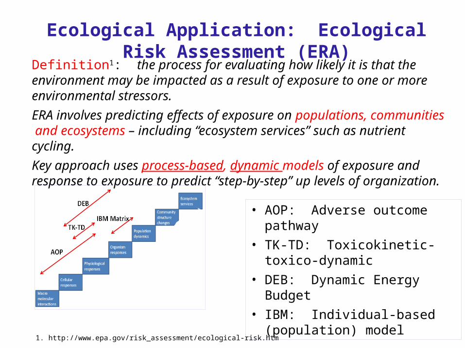
Definition1: the process for evaluating how likely it is that the environment may be impacted as a result of exposure to one or more environmental stressors.ERA involves predicting effects of exposure on populations, communities and ecosystems – including “ecosystem services” such as nutrient cycling. Key approach uses process-based, dynamic models of exposure and response to exposure to predict “step-by-step” up levels of organization.
1. http://www.epa.gov/risk_assessment/ecological-risk.htm
• AOP: Adverse outcome pathway• TK-TD: Toxicokinetic-toxico-dynamic• DEB: Dynamic Energy Budget • IBM: Individual-based (population)
model
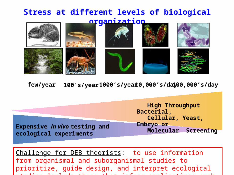
100’s/year 1000’s/year 10,000’s/day 100,000’s/day
High Throughput Bacterial, Cellular, Yeast, Embryo or Molecular Screening
Stress at different levels of biological organization
Expensive in vivo testing and ecological experiments
few/year
Challenge for DEB theorists: to use information from organismal and suborganismal studies to prioritize, guide design, and interpret ecological studies Include those that inform applications such as ERA.

Environmental Challenges are Urgent
• Climate change effects already occur and will accelerate over decades• Environmental Stress is rapid (e.g. nutrient enrichment, insecticides,
water supply, frequency of extreme events)• Technology changes rapidly(e.g. engineered nanomaterials)
YET• DEB is over 30 years old and had its origins in ecotoxicology, but only
a very few agencies or industries use it, in spite of focused publications (e.g. OECD guidance document)
IMPLYING• EITHER: DEB is “too complicated” for practical applications• OR: We (DEB crowd) need to improve communication
Meeting the challenges
DEB is “too complicated” for practical applications• Often true (unfortunately) • “Keep it simple”, but NOT stupid• Use both DEB-based and DEB-inspired models
Improving communication• Know intellectual culture of users (e.g. ecology or
ecotoxicogy)• Develop useful tools

DEB-BASED POPULATION MODELS
Two approaches to modeling population dynamics
A population is a collection of individual organisms interacting with a shared environment.
Individual-based models (IBMs). Simulate a large number of individuals, each obeying the rules of a DEB model (i-state dynamics).
• Structured population models. This involves modeling the distribution of individuals among i-states. A large body of theory has been developed1, and there is a powerful computational approach – the “escalator boxcar train”2. .
1. See for example many papers by J.A.J. Metz, O. Diekmann, A.M. de Roos
2. See http://staff.science.uva.nl/~aroos/EBT/index.html
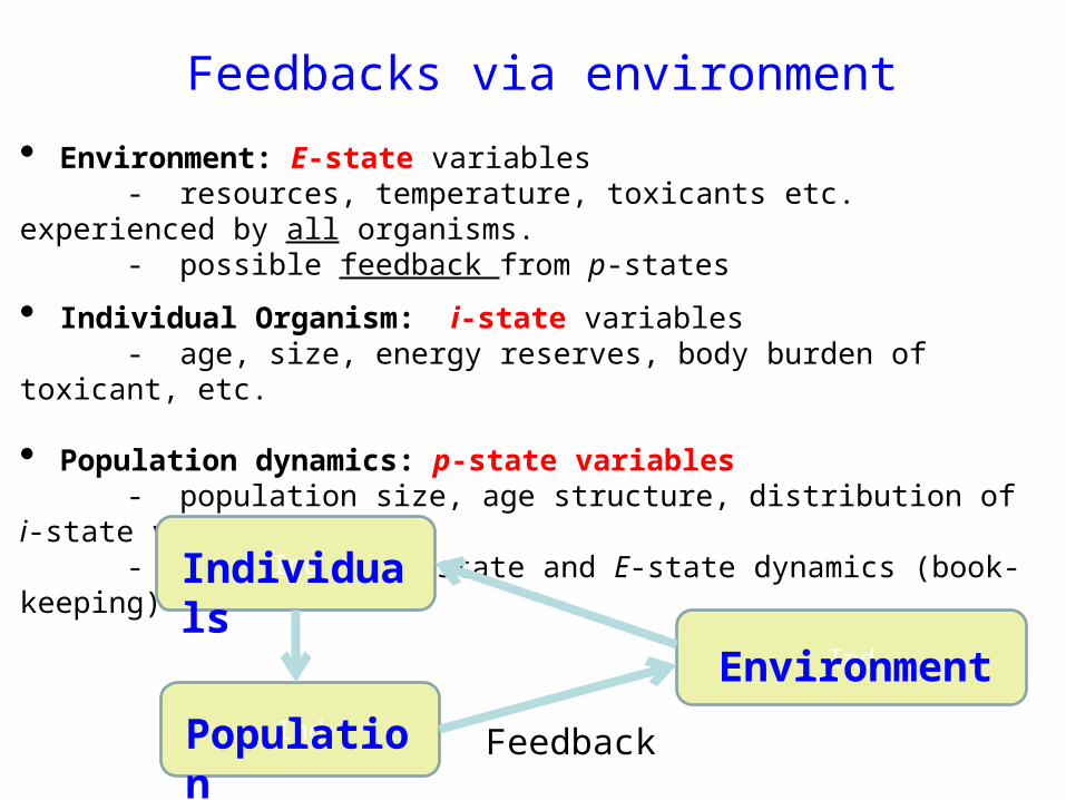
Feedbacks via environment
• Environment: E-state variables - resources, temperature, toxicants etc. experienced by all organisms. - possible feedback from p-states
• Individual Organism: i-state variables - age, size, energy reserves, body burden of toxicant, etc.
• Population dynamics: p-state variables - population size, age structure, distribution of i-state variables - derived from i-state and E-state dynamics (book-keeping)
IndIndividuals
IndEnvironment
IndPopulation Feedback
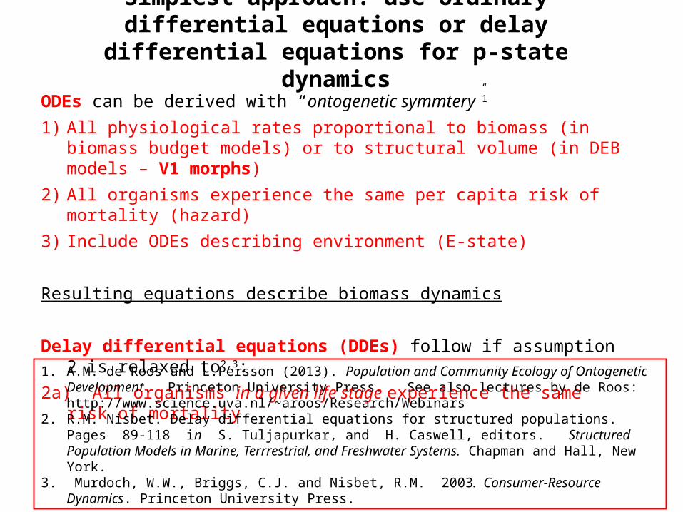
Simplest approach: use ordinary differential equations or delay differential equations for p-state
dynamics
ODEs can be derived with “ontogenetic symmtery”1
1) All physiological rates proportional to biomass (in biomass budget models) or to structural volume (in DEB models – V1 morphs)
2) All organisms experience the same per capita risk of mortality (hazard)
3) Include ODEs describing environment (E-state)
Resulting equations describe biomass dynamics
Delay differential equations (DDEs) follow if assumption 2 is relaxed to2,3:
2a) All organisms in a given life stage experience the same risk of mortality
1. A.M. de Roos and L.Persson (2013). Population and Community Ecology of Ontogenetic Development. Princeton University Press. See also lectures by de Roos: http://www.science.uva.nl/~aroos/Research/Webinars
2. R.M. Nisbet. Delay differential equations for structured populations. Pages 89-118 in S. Tuljapurkar, and H. Caswell, editors. Structured Population Models in Marine, Terrrestrial, and Freshwater Systems. Chapman and Hall, New York.
3. Murdoch, W.W., Briggs, C.J. and Nisbet, R.M. 2003. Consumer-Resource Dynamics. Princeton University Press.
Population dynamics and bioenergetics – two bodies of coherent theory
Coming soon – de Roos keynote!
DEB Biomass –based models

DEB-based IBMs*
* B.T. Martin, E.I. Zimmer, V. Grimm and T. Jager (2012). Methods in Ecology and Evolution 3: 445-449
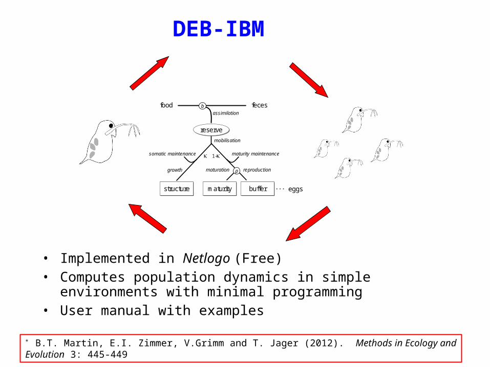
DEB-IBM
structurestructure
food feces
maturity maintenancesomatic maintenance
assimilation
1-
growth reproduction
maturitymaturity bufferbuffer
maturation
b
p
reservereserve
mobilisation
eggs
• Implemented in Netlogo (Free) • Computes population dynamics in simple environments with minimal
programming • User manual with examples
* B.T. Martin, E.I. Zimmer, V.Grimm and T. Jager (2012). Methods in Ecology and Evolution 3: 445-449

Population model tests*
* B.T. Martin, T. Jager, R.M. Nisbet, T.G. Preuss, V. Grimm(2013). Predicting population dynamics from the properties of individuals: a cross-level test of Dynamic Energy Budget theory. American Naturalist, 181:506-519.
Low food (0.5mgC d-1)
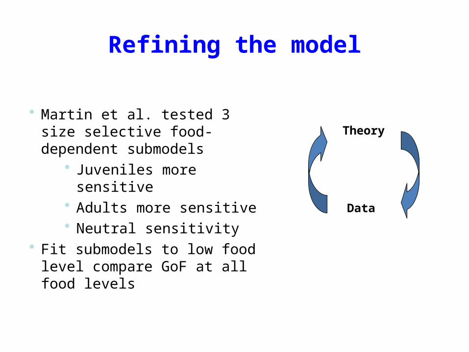
Refining the model
• Martin et al. tested 3 size selective food-dependent submodels
• Juveniles more sensitive• Adults more sensitive• Neutral sensitivity
• Fit submodels to low food level compare GoF at all food levels
Theory
Data
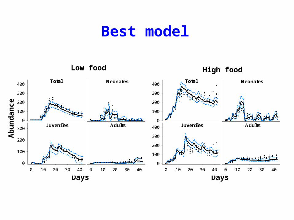
Best model
Total
0
100
200
300
400
Juveniles
0 10 20 30 40
0
100
200
300
Neonates
Adults
0 10 20 30 40
Total
0
100
200
300
400
Juveniles
0 10 20 30 400
100
200
300
400
Neonates
Adults
0 10 20 30 40
High foodLow food
Days Days
Abun
danc
e
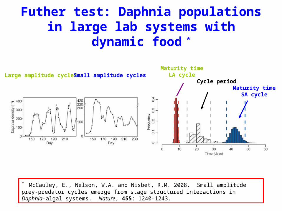
Futher test: Daphnia populations in large lab systems with dynamic food *
Maturity timeLA cycle
Cycle periodMaturity time
SA cycle
Large amplitude cycles Small amplitude cycles
* McCauley, E., Nelson, W.A. and Nisbet, R.M. 2008. Small amplitude prey-predator cycles emerge from stage structured interactions in Daphnia-algal systems. Nature, 455: 1240-1243.
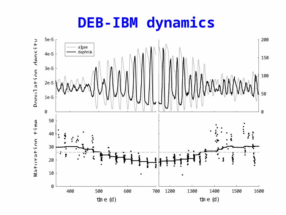
DEB-IBM dynamics
2D Graph 1
time (d)
1200 1300 1400 1500 1600
0
1e-5
2e-5
3e-5
4e-5
5e-5
Col 9 vs Col 10 Col 9 vs Col 11
time (d)
400 500 600 7000
10
20
30
40
50
0
50
100
150
200
algaedaphnia
Mat
urati
on ti
me
Popu
latio
n de
nsity
leng
th (
mm
)
0
1
2
3
4
5
time (d)
0 5 10 15 20
cum
ulat
ive
repr
oduc
tion
0
25
50
75
100
125
150
175
MaturationReproductionGrowth
Somatic maintenance
Maturity maintenance
x
Feeding
leng
th (
mm
)
0
1
2
3
4
5
time (d)
0 5 10 15 20
cum
ulat
ive
repr
oduc
tion
0
25
50
75
100
125
150
175
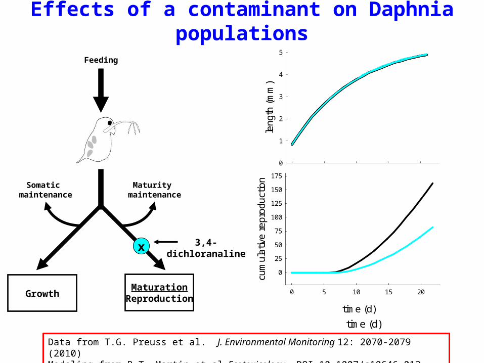
3,4-dichloranaline
Effects of a contaminant on Daphnia populations
Data from T.G. Preuss et al. J. Environmental Monitoring 12: 2070-2079 (2010)Modeling from B.T. Martin et al. Ecotoxicology, DOI 10.1007/s10646-013-1049-x (2013)
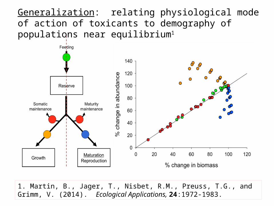
Generalization: relating physiological mode of action of toxicants to demography of populations near equilibrium1
1. Martin, B., Jager, T., Nisbet, R.M., Preuss, T.G., and Grimm, V. (2014). Ecological Applications, 24:1972-1983.
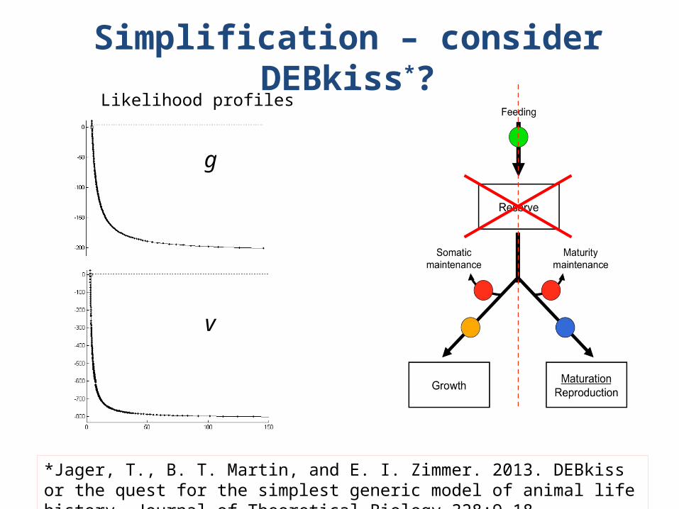
Simplification – consider DEBkiss*?
*Jager, T., B. T. Martin, and E. I. Zimmer. 2013. DEBkiss or the quest for the simplest generic model of animal life history. Journal of Theoretical Biology 328:9-18.
Likelihood profiles
g
v
DEB-INSPIRED MODEL OF FEEDBACKS
INVOLVING METABOLIC PRODUCTS
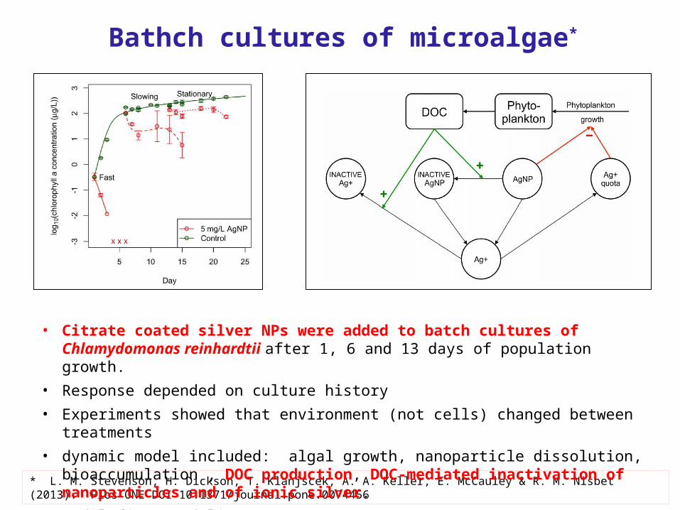
Bathch cultures of microalgae*
* L. M. Stevenson, H. Dickson, T. Klanjscek, A. A. Keller, E. McCauley & R. M. Nisbet (2013). Plos ONE DOI 10.1371/journal.pone.0074456
• Citrate coated silver NPs were added to batch cultures of Chlamydomonas reinhardtii after 1, 6 and 13 days of population growth.
• Response depended on culture history
• Experiments showed that environment (not cells) changed between treatments
• dynamic model included: algal growth, nanoparticle dissolution, bioaccumulation , DOC production, DOC-mediated inactivation of nanoparticles and of ionic silver.
• Model fits (red lines)
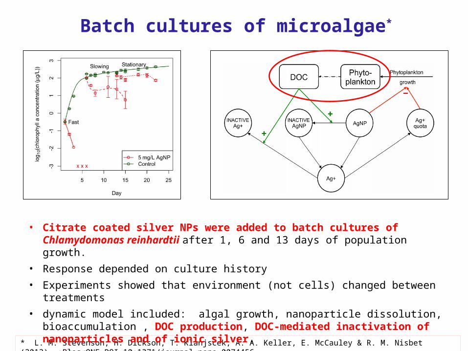
Batch cultures of microalgae*
* L. M. Stevenson, H. Dickson, T. Klanjscek, A. A. Keller, E. McCauley & R. M. Nisbet (2013). Plos ONE DOI 10.1371/journal.pone.0074456
• Citrate coated silver NPs were added to batch cultures of Chlamydomonas reinhardtii after 1, 6 and 13 days of population growth.
• Response depended on culture history
• Experiments showed that environment (not cells) changed between treatments
• dynamic model included: algal growth, nanoparticle dissolution, bioaccumulation , DOC production, DOC-mediated inactivation of nanoparticles and of ionic silver.
• Model fits (red lines)
88888
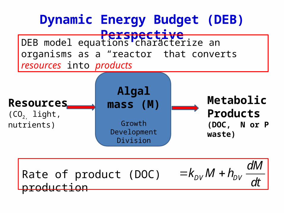
Dynamic Energy Budget (DEB) Perspective
Algal mass (M)
GrowthDevelopment
Division
Resources(CO2, light, nutrients)
Metabolic Products(DOC, N or P waste)
DEB model equations characterize an organisms as a “reactor” that converts resources into products
DV DV
dMk M h
dt Rate of product (DOC) production
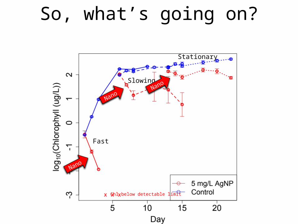
Fast
Slowing
Stationary
Chl below detectable limit
So, what’s going on?
NanoNano
Nano

Fast
Slowing
Stationary
Chl below detectable limit
So, what’s going on?
NanoNano
Nano
Nano
+Ionic
Nano
+Ionic
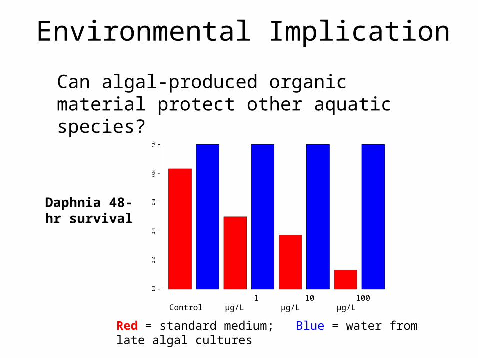
Environmental Implication
Control 1 μg/L
10 μg/L 100 μg/L
Can algal-produced organic material protect other aquatic species?
Daphnia 48-hr survival
Red = standard medium; Blue = water from late algal cultures

DEB theory for communities
• Community: collection of interacting species
• Ecosystem: Focus on energy and material flows among groups of species (e.g. trophic levels).
• Overarching challenge – understanding biodiversity
Communities and Ecosystems
• Community dynamics involves much more than bioenergetic processes .
• No consensus on whether “biology matters” – neutral theory
• Is DEB relevant?

RESOURCE COMPETITION
A little demography
Consider a population of females divided into discrete age classes Let aS be the fraction of newborns that survive to age a
Let a be the total number of offspring from individual aged a .
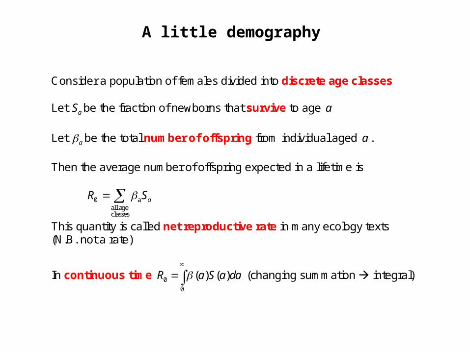
A little demography
Consider a population of females divided into discrete age classes Let aS be the fraction of newborns that survive to age a
Let a be the total number of offspring from individual aged a .
Then the average number of offspring expected in a lifetime is 0 a
all ageclasses
aR S
This quantity is called net reproductive rate in many ecology texts (N.B. not a rate)
In continuous time 0
0
( ) ( )R a S a da
(changing summation integral)
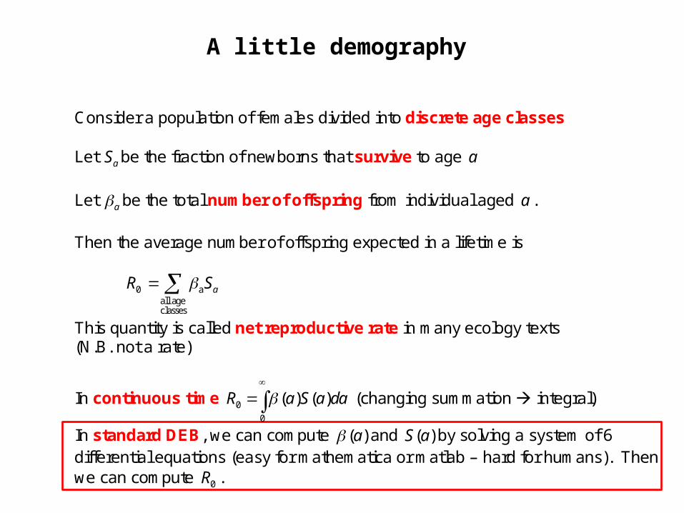
In standard DEB, we can compute ( )a and ( )S a by solving a system of 6 differential equations (easy for mathematica or matlab – hard for humans). Then we can compute 0R .
A little population ecology
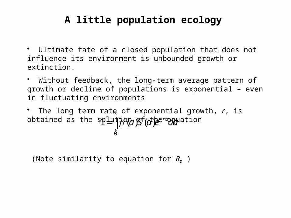
• Ultimate fate of a closed population that does not influence its environment is unbounded growth or extinction.
• Without feedback, the long-term average pattern of growth or decline of populations is exponential – even in fluctuating environments
• The long term rate of exponential growth, r, is obtained as the solution of the equation
(Note similarity to equation for R0 )0
1 ( ) ( ) raa S a e da
A little population ecology
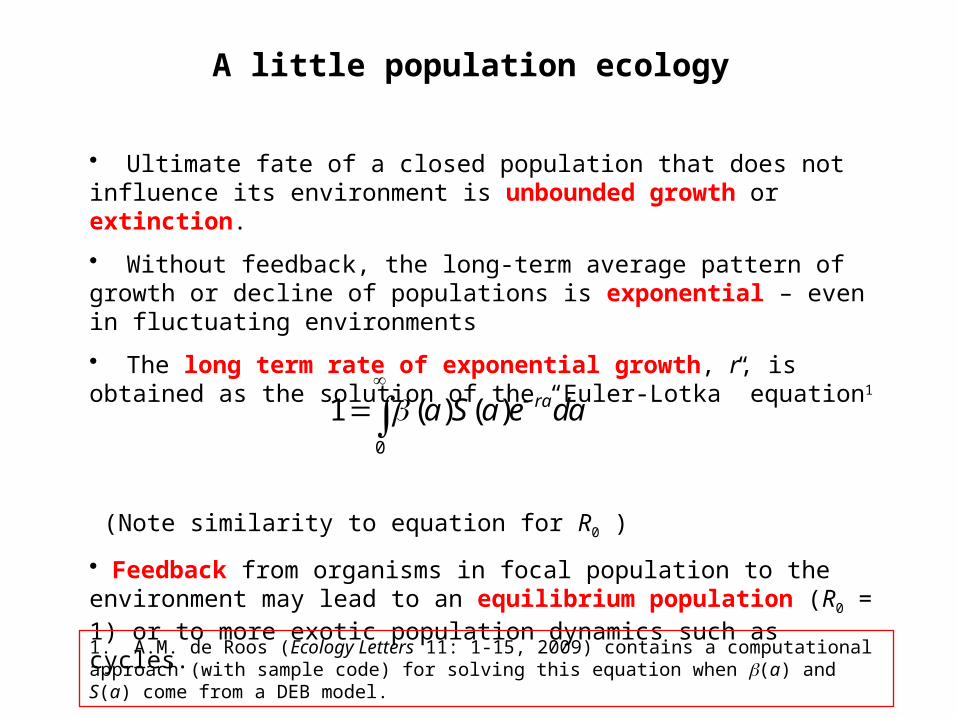
• Ultimate fate of a closed population that does not influence its environment is unbounded growth or extinction.
• Without feedback, the long-term average pattern of growth or decline of populations is exponential – even in fluctuating environments
• The long term rate of exponential growth, r, is obtained as the solution of the “Euler-Lotka” equation1
(Note similarity to equation for R0 )
• Feedback from organisms in focal population to the environment may lead to an equilibrium population (R0 = 1) or to more exotic population dynamics such as cycles.
0
1 ( ) ( ) raa S a e da
1. A.M. de Roos (Ecology Letters 11: 1-15, 2009) contains a computational approach (with sample code) for solving this equation when b(a) and S(a) come from a DEB model.
Resource competition
Consider two species competing for a single food resource, X.
For each species, R0 is a function of X., and at equilibrium, R0=1.
Thus equilibrium coexistence is unlikely.
Idea behind competitive exclusion principle
Resource competition
Consider two species competing for a single food resource, X.
For each species, R0 is a function of X., and at equilibrium, R0=1.
Thus equilibrium coexistence is unlikely.
Idea behind competitive exclusion principle (CEP)
Coexistence at equilibrium of N species requires N resources

Theory behind CEP is soundDavid Tilman (1977) Resource Competition between Plankton Algae: An Experimental and Theoretical Approach. Ecology, 58, 338-348.
• 2 algal species, 2 substrates (P and Si);• Described by Droop model (evolutionary ancestor of DEB)• Chemostat dynamics + labe experiments• Field data from Lake Michigan
LAB LAKE

Possible mechanisms for species coexistence
DEB3 page 337

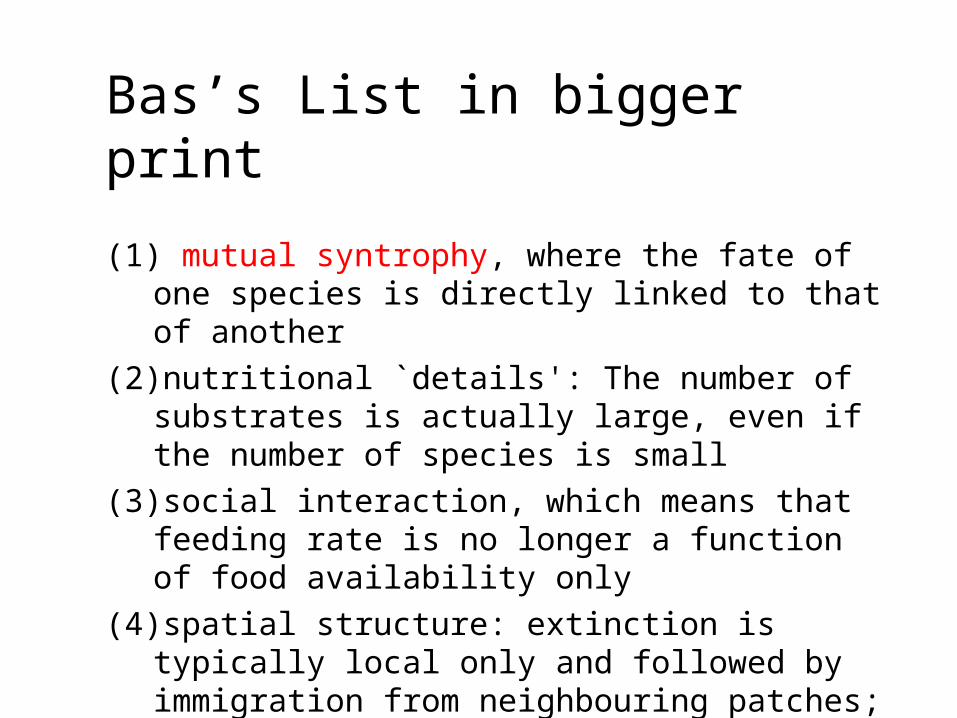
Bas’s List in bigger print
(1) mutual syntrophy, where the fate of one species is directly linked to that of another
(2) nutritional `details': The number of substrates is actually large, even if the number of species is small
(3) social interaction, which means that feeding rate is no longer a function of food availability only
(4) spatial structure: extinction is typically local only and followed by immigration from neighbouring patches;
(5) temporal structure
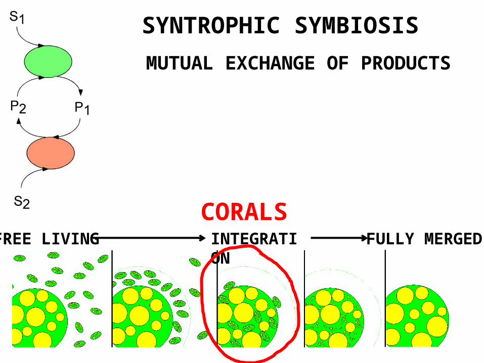
SYNTROPHIC SYMBIOSIS
INTEGRATION FULLY MERGEDFREE LIVING
MUTUAL EXCHANGE OF PRODUCTS
CORALS

FREE LIVING H
OST
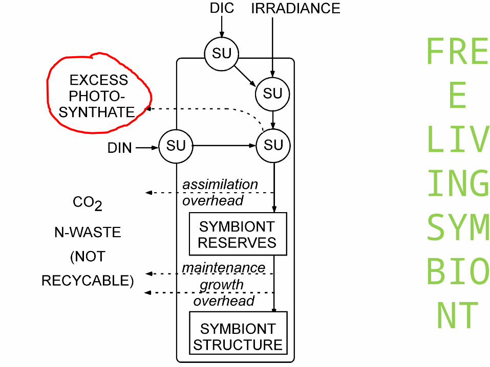
FREE LIVING
SYMBIONT
END
OSYMBIOSIS
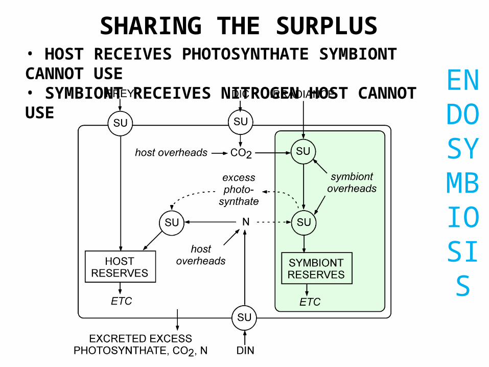
SHARING THE SURPLUS• HOST RECEIVES PHOTOSYNTHATE SYMBIONT CANNOT USE• SYMBIONT RECEIVES NITROGEN HOST CANNOT USE
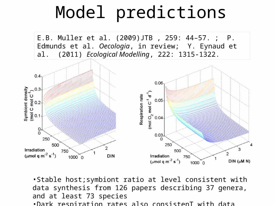
Model predictionsE.B. Muller et al. (2009)JTB , 259: 44–57. ; P. Edmunds et al. Oecologia, in review; Y. Eynaud et al. (2011) Ecological Modelling, 222: 1315-1322.
•Stable host;symbiont ratio at level consistent with data synthesis from 126 papers describing 37 genera, and at least 73 species•Dark respiration rates also consistenT with data
Bas’s List in bigger print
(1) mutual syntrophy, where the fate of one species is directly linked to that of another
(2) nutritional `details': The number of substrates is actually large, even if the number of species is small
(3) social interaction, which means that feeding rate is no longer a function of food availability only
(4) spatial structure: extinction is typically local only and followed by immigration from neighbouring patches;
(5) temporal structure
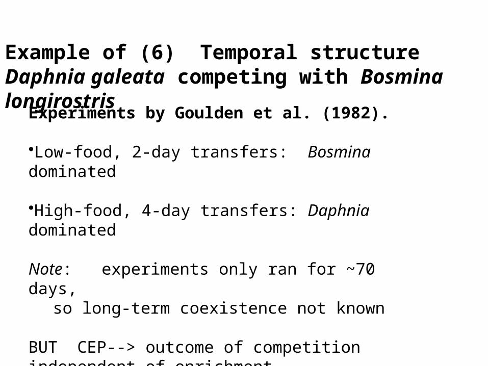
Example of (6) Temporal structure Daphnia galeata competing with Bosmina longirostris
Experiments by Goulden et al. (1982).
•Low-food, 2-day transfers: Bosmina dominated
•High-food, 4-day transfers: Daphnia dominated
Note: experiments only ran for ~70 days, so long-term coexistence not known
BUT CEP--> outcome of competition independent of enrichment.
EXPLANATION: Temporal variability due to experimenter!
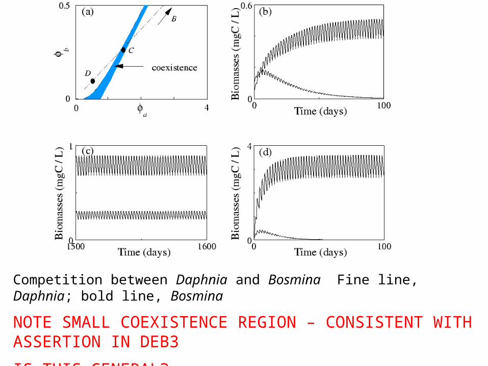
Competition between Daphnia and Bosmina Fine line, Daphnia; bold line, Bosmina
NOTE SMALL COEXISTENCE REGION – CONSISTENT WITH ASSERTION IN DEB3
IS THIS GENERAL?
