deblurring natural image using super-gaussian fieldsopenaccess.thecvf.com › ... ›...

Deblurring Natural Image Using Super-Gaussian Fields

Yuhang Liu1(https://orcid.org/0000-0002-8195-9349), Wenyong Dong1, Dong Gong2,

Lei Zhang2, and Qinfeng Shi2

1Computer School, Wuhan University, Hubei, China

{liuyuhang, dwy}@whu.edu.cn2School of Computer Science, The University of Adelaide, Adelaide, Australia

{dong.gong, lei.zhang, javen.shi}@adelaide.edu.au

Abstract. Blind image deblurring is a challenging problem due to its ill-posed

nature, of which the success is closely related to a proper image prior. Although

a large number of sparsity-based priors, such as the sparse gradient prior, have

been successfully applied for blind image deblurring, they inherently suffer from

several drawbacks, limiting their applications. Existing sparsity-based priors are

usually rooted in modeling the response of images to some specific filters (e.g.,

image gradients), which are insufficient to capture the complicated image struc-

tures. Moreover, the traditional sparse priors or regularizations model the filter

response (e.g., image gradients) independently and thus fail to depict the long-

range correlation among them. To address the above issues, we present a novel

image prior for image deblurring based on a Super-Gaussian field model with

adaptive structures. Instead of modeling the response of the fixed short-term fil-

ters, the proposed Super-Gaussian fields capture the complicated structures in

natural images by integrating potentials on all cliques (e.g., centring at each pixel)

into a joint probabilistic distribution. Considering that the fixed filters in different

scales are impractical for the coarse-to-fine framework of image deblurring, we

define each potential function as a super-Gaussian distribution. Through this def-

inition, the partition function, the curse for traditional MRFs, can be theoretically

ignored, and all model parameters of the proposed Super-Gaussian fields can be

data-adaptively learned and inferred from the blurred observation with a varia-

tional framework. Extensive experiments on both blind deblurring and non-blind

deblurring demonstrate the effectiveness of the proposed method.

1 Introduction

Image deblurring involves the estimation of a sharp image when given a blurred obser-

vation. Generally, this problem can be formalized as follows:

y = k⊗ x+ n, (1)

where the blurred image y is generated by convolving the latent image x with a blur

kernel k, ⊗ denotes the convolution operator, and n denotes the noise corruption. When

the kernel k is unknown, the problem is termed blind image deblurring (BID), and

conversely, the non-blind image deblurring (NBID). It has been shown that both of these

two problems are highly ill-posed. Thus, to obtain meaningful solutions, appropriate

priors on latent image x is necessary.

2 Y. Liu, W. Dong, D. Gong, L. Zhang, and Q. Shi

(a) (b) (c) (d) (e)

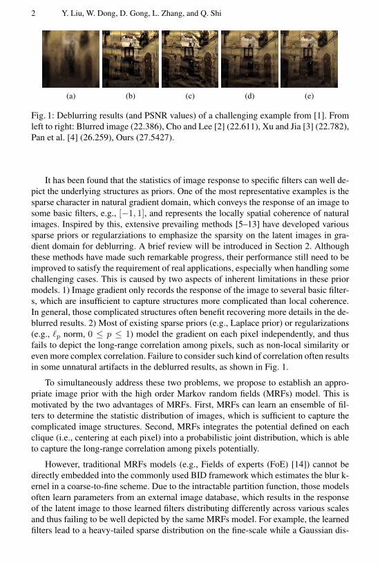
Fig. 1: Deblurring results (and PSNR values) of a challenging example from [1]. From

left to right: Blurred image (22.386), Cho and Lee [2] (22.611), Xu and Jia [3] (22.782),

Pan et al. [4] (26.259), Ours (27.5427).

It has been found that the statistics of image response to specific filters can well de-

pict the underlying structures as priors. One of the most representative examples is the

sparse character in natural gradient domain, which conveys the response of an image to

some basic filters, e.g., [−1, 1], and represents the locally spatial coherence of natural

images. Inspired by this, extensive prevailing methods [5–13] have developed various

sparse priors or regularziations to emphasize the sparsity on the latent images in gra-

dient domain for deblurring. A brief review will be introduced in Section 2. Although

these methods have made such remarkable progress, their performance still need to be

improved to satisfy the requirement of real applications, especially when handling some

challenging cases. This is caused by two aspects of inherent limitations in these prior

models. 1) Image gradient only records the response of the image to several basic filter-

s, which are insufficient to capture structures more complicated than local coherence.

In general, those complicated structures often benefit recovering more details in the de-

blurred results. 2) Most of existing sparse priors (e.g., Laplace prior) or regularizations

(e.g., ℓp norm, 0 ≤ p ≤ 1) model the gradient on each pixel independently, and thus

fails to depict the long-range correlation among pixels, such as non-local similarity or

even more complex correlation. Failure to consider such kind of correlation often results

in some unnatural artifacts in the deblurred results, as shown in Fig. 1.

To simultaneously address these two problems, we propose to establish an appro-

priate image prior with the high order Markov random fields (MRFs) model. This is

motivated by the two advantages of MRFs. First, MRFs can learn an ensemble of fil-

ters to determine the statistic distribution of images, which is sufficient to capture the

complicated image structures. Second, MRFs integrates the potential defined on each

clique (i.e., centering at each pixel) into a probabilistic joint distribution, which is able

to capture the long-range correlation among pixels potentially.

However, traditional MRFs models (e.g., Fields of experts (FoE) [14]) cannot be

directly embedded into the commonly used BID framework which estimates the blur k-

ernel in a coarse-to-fine scheme. Due to the intractable partition function, those models

often learn parameters from an external image database, which results in the response

of the latent image to those learned filters distributing differently across various scales

and thus failing to be well depicted by the same MRFs model. For example, the learned

filters lead to a heavy-tailed sparse distribution on the fine-scale while a Gaussian dis-

Deblurring Natural Image Using Super-Gaussian Fields 3

tribution on the coarse scale. That is one of the inherent reasons for why MRFs model

is rarely employed for BID.

To overcome this difficulty, we propose a novel MRFs based image prior, termed

super-Gaussian fields (SGF), where each potential is defined as a super-Gaussian dis-

tribution. By doing this, the partition function, the curse for traditional MRFs, can be

theoretically ignored during parameter learning. With this advantage, the proposed M-

RF model can be seamlessly integrated into the coarse-to-fine framework, and all model

parameters, as well as the latent image, can be data-adaptively learned and inferred from

the blurred observation with a variational framework. Compared with prevailing deblur-

ring methods on extensive experiments, the proposed method shows obvious superiority

under both BID and NBID settings.

2 Related Work

2.1 Blind Image Deblurring

Due to the pioneering work of Fergus et al. [5] that imposes sparsity on image in the

gradient spaces, sparse priors have attracted attention [5–13]. For example, a mixture

of Gaussian models is early used to chase the sparsity due to its excellent approximate

capability [5, 6]. A total variation model is employed since it can encourage gradient

sparsity [7, 8]. A student-t prior is utilized to impose the sparsity [9]. A super-Gaussian

model is introduced to represent a general sparse prior [10]. Those priors are limited by

the fact that they are related to the l1-norm. To relax the limitation, many the lp-norm

(where p < 1) based priors are introduced to impose sparsity on image [11–13]. For

example, Krishnan et al. [11] propose a normalized sparsity prior (l1/l2). Xu et al. [12]

propose a new sparse l0 approximation. Ge et al. [13] introduce a spike-and-slab prior

that corresponds to the l0-norm. However, all those priors are limited by the fact that

they assume the coefficients in the gradient spaces are mutually independent.

Besides the above mentioned sparse priors, a family of blind deblurring approaches

explicitly exploits the structure of edges to estimate the blur kernel [2, 3, 15–19]. Joshi et

al. [16] and Cho et al. [15] rely on restoring edges from the blurry image. However, they

fail to estimate the blur kernel with large size. To remedy it, Cho and Lee [2] alternately

recover sharp edges and the blur kernel in a coarse-to-fine fashion. Xu and Jia [3] further

develop this work. However, these approaches heavily rely on empirical image filters.

To avoid it, Sun et al. [17] explore the edges of natural images using learned patch prior.

Lai et al. [18] predict the edges by learned prior. Zhou and Komodakis [19] detect edges

using a high-level scene-specific prior. All those priors only explore the local patch in

the latent image but neglect the global characters.

Rather than exploiting edges, there are many other priors. Komodakis and Paragios

[20] explore the quantized version of the sharp image by a discrete MRF prior. Their

MRF prior is different with the proposed SG-FoE prior that is a continuous MRF prior.

Michaeli and Irani [21] seek sharp image by the recurrence of small image patches.

Gong et al. [22, 23] hire a subset of the image gradients for kernel estimation. Pan et

al. [4] and Yan et al. [24] explore dark and bright pixels for BID, respectively. Besides,

deep learning based methods have been adopted recently [25, 26].


2.2 High-Order MRFs for Image Modeling

Since gradient filters only model the statistics of first derivatives in the image struc-

ture, high-order MRF generalizes traditional based-gradient pairwise MRF models, e.g.,

cluster sparsity field [27], by defining linear filters on large maximal cliques. Based on

the Hammersley-Clifford theorem [28], high-order MRF can give the general form to

model image as follows:

p(x;Θ) =1

Z(Θ)

∏c∈C

J∏j=1

φ(Jjxc), (2)

where C are the maximal cliques, xc are the pixels of clique c, Jj are the linear filters

and j = 1, ..., J , Z(Θ) is the partition function with parameters Θ that depend on φand Jj , φ are the potentials. In contrast to previous high-order MRF in which the model

parameters are hand-defined, FoE [14], a class of high-order MRF, can learn the model

parameters from an external database, and hence has attracted high attention in image

denoising [29, 30], NBID [31] and image super resolution [32].

3 Image Modeling with Super-Gaussian Fields

In this section, we first figure out the reason why traditional high-order MRFs mod-

els cannot be directly embedded into the coarse-to-fine deblurring framework. To this

end, we comprehensively investigate a typical high-order MRF model, Gaussian scale

mixture-FoE model (GSM-FoE) [29], and finally find out its inherent limitation. Then,

we propose a super-Gaussian Fields based image prior model and analyze its properties.

3.1 Blind Image Deblurring with GSM-FoE

According to [29], GSM-FoE follows the general MRFs form in (2) and defines each

potential with GSM as follows:

φ(Jjxc;αj,k) =∑K

k=1αj,kN (Jjxc; 0, ηj/sk), (3)

where N (Jjxc; 0, ηj/sk) denotes the Gaussian probability density function with zero

mean and variance ηj/sk. sk and αj,k denote the scale and weight parameters, respec-

tively. It has been shown that GSM-FoE can well depict the sparse and wide heavy-

tailed distributions [29]. Similar as most previous MRFs models, the partition function

Z(Θ) for GSM-FoE is generally intractable since it requires integrating over all possi-

ble images. However, evaluating Z(Θ) is necessitated to learn all the model parameters,

e.g., {Jj} and {αj,k} (ηj and sk are generally constant). To sidestep this difficulty, most

MRFs models including GSM-FoE turn to learn model parameters by maximizing the

likelihood in (2) on an external image database [14, 29, 30], and then apply the learned

model in the following applications, e.g., image denoising, super-resolution etc.

However, the pre-learned GSM-FoE cannot be directly employed to BID. This is

because of that BID commonly adopts a coarse-to-fine framework, while the responses


Original scale-0.4 -0.2 0 0.2 0.4 0.6

log

2 p

rob

ab

ility

de

nsity

-20

-15

-10

-5

0

0.7171 scale-0.4 -0.2 0 0.2 0.4 0.6

log

2 p

rob

ab

ility

de

nsity

-15

-10

-5

0

0.5 scale-0.4 -0.2 0 0.2 0.4 0.6

log

2 p

rob

ab

ility

de

nsity

-14

-12

-10

-8

-6

-4

-2

0

0.3535 scale-0.4 -0.2 0 0.2 0.4 0.6

log

2 p

rob

ab

ility

de

nsity

-14

-12

-10

-8

-6

-4

-2

0

0.25 scale-0.4 -0.2 0 0.2 0.4 0.6

log

2 p

rob

ab

ility

de

nsity

-12

-10

-8

-6

-4

-2

0

Sharp image

Heavy tailsHeavy tails

Heavy tails

No tailsNo tails

(a) (b) (c) (d)

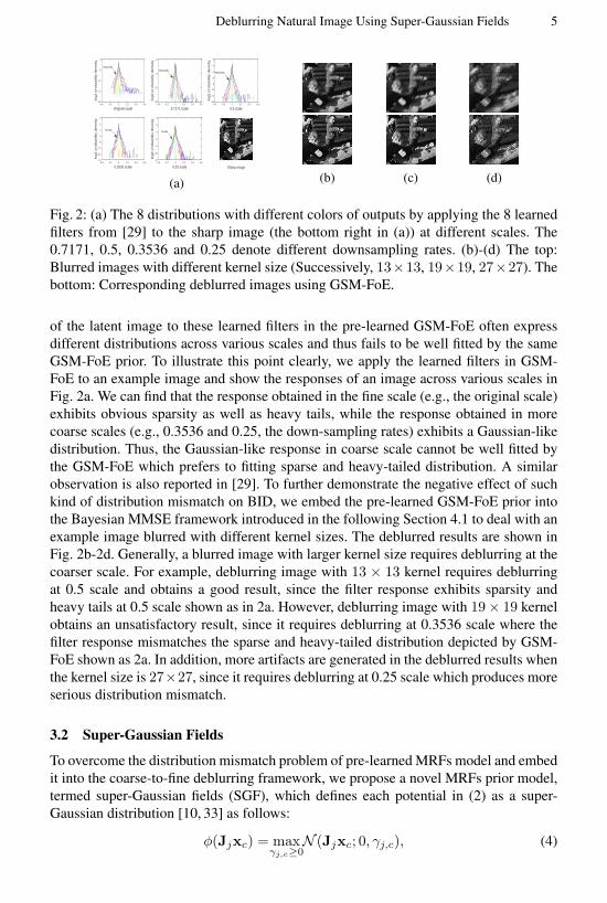
Fig. 2: (a) The 8 distributions with different colors of outputs by applying the 8 learned

filters from [29] to the sharp image (the bottom right in (a)) at different scales. The

0.7171, 0.5, 0.3536 and 0.25 denote different downsampling rates. (b)-(d) The top:

Blurred images with different kernel size (Successively, 13×13, 19×19, 27×27). The

bottom: Corresponding deblurred images using GSM-FoE.

of the latent image to these learned filters in the pre-learned GSM-FoE often express

different distributions across various scales and thus fails to be well fitted by the same

GSM-FoE prior. To illustrate this point clearly, we apply the learned filters in GSM-

FoE to an example image and show the responses of an image across various scales in

Fig. 2a. We can find that the response obtained in the fine scale (e.g., the original scale)

exhibits obvious sparsity as well as heavy tails, while the response obtained in more

coarse scales (e.g., 0.3536 and 0.25, the down-sampling rates) exhibits a Gaussian-like

distribution. Thus, the Gaussian-like response in coarse scale cannot be well fitted by

the GSM-FoE which prefers to fitting sparse and heavy-tailed distribution. A similar

observation is also reported in [29]. To further demonstrate the negative effect of such

kind of distribution mismatch on BID, we embed the pre-learned GSM-FoE prior into

the Bayesian MMSE framework introduced in the following Section 4.1 to deal with an

example image blurred with different kernel sizes. The deblurred results are shown in

Fig. 2b-2d. Generally, a blurred image with larger kernel size requires deblurring at the

coarser scale. For example, deblurring image with 13 × 13 kernel requires deblurring

at 0.5 scale and obtains a good result, since the filter response exhibits sparsity and

heavy tails at 0.5 scale shown as in 2a. However, deblurring image with 19× 19 kernel

obtains an unsatisfactory result, since it requires deblurring at 0.3536 scale where the

filter response mismatches the sparse and heavy-tailed distribution depicted by GSM-

FoE shown as 2a. In addition, more artifacts are generated in the deblurred results when

the kernel size is 27×27, since it requires deblurring at 0.25 scale which produces more

serious distribution mismatch.

3.2 Super-Gaussian Fields

To overcome the distribution mismatch problem of pre-learned MRFs model and embed

it into the coarse-to-fine deblurring framework, we propose a novel MRFs prior model,

termed super-Gaussian fields (SGF), which defines each potential in (2) as a super-

Gaussian distribution [10, 33] as follows:

φ(Jjxc) = maxγj,c≥0

N (Jjxc; 0, γj,c), (4)


where γj,c denotes the variance. Similar to GSM, SG also can depict sparse and heavy-

tailed distributions [33]. Different from GSM-FoE and most MRFs models, the partition

function in super-Gaussian fields can be ignored during parameter learning. More im-

portantly, with such an advantage, it is possible to learn its model parameters directly

from the blurred observation in each scale, and thus the proposed super-Gaussian fields

can be seamlessly embedded into the coarse-to-fine deburring framework. In the fol-

lowing, we give the theoretical results to ignore the partition function in details.

Property 1. The potential φ of SGF is related to Jj and xc, but not γj,c. Hence, the

partition function Z(Θ) of SGF just depends on the linear filters Jj .

Proof. As shown in (4), γj,c can be determined by Jj and xc. Hence, the potential φ in

(4) is related to only Jj and xc. Furthermore, because Z(Θ) =∫ ∏

c∈C

∏J

j=1 φ(Jjxc)dx

, the partition function Z(Θ) just depends on the linear filters Jj once the integral is

done. Namely, Θ = {Jj |j = 1, ..., J}.

Property 2. Given any set of J orthonormal vectors {VJj}, {VJ′

j}, VJj

denote the

vectored version of the linear filters Jj (VJjis the vector formed through the concate-

nation of vectors of Jj .), for the partition function of SGF: Z({VJj}) = Z({VJ′

j}).

To proof Property 2, we first introduce the following theory,

Theorem 1 ([30]) Let E(VTJjTx) be an arbitrary function of VT

JjTx and define Z(V) =∫

e−

∑jE(VT

JjTx)dx, where Tx denotes the Toeplitz (convolution) matrix (e.g., Jj ⊗

x = VTJjTx.) with x. Then Z(V) = Z(V′) for any set of J orthonormal vectors

{VJj}, {V′

Jj} .

Proof (to Property 2). Since the partition function Z(Θ) of SGF just depends on the

linear filters {JJj} as mentioned in Property 1 and the potential φ in (4) also perfectly

meets the form of E(VTJjTx) in Theorem 1, it is easy to proof Property 2.

Based on Property 1, we do not need to evaluate the partition function Z(Θ) of

SGF to straightforward update γj,c, since Z(Θ) do not depend on γj,c. Further, based

on Property 2, we can also do not need evaluate Z(Θ) of SGF to update Jj , if we limit

updating Jj in the orthonormal space.

4 Image Deblurring with the Proposed SGF

In this section, we first propose a iterative method with SGF to handle BID in an coarse-

to-fine scheme. We then show how to extend the proposed to non-blind image deblur-

ring and non-uniform blind image deblurring.

4.1 Blind Image Deblurring with SGF

Based on the proposed SGF, namely (2) and (4), we propose a novel approach for BID

in this section. In contrast to some existing methods which can only estimate the blur

kernel, our approach can simultaneously recover latent image and the blur kernel. We

will further discuss it in Section 4.2.


Recovering Latent Image Given the blur kernel, a conventional approach to recover

latent image is Maximum a Posteriori (MAP) estimation. However, MAP favors the

no-blur solution due to the influence of image size [34]. To overcome it, we introduce

Bayesian MMSE to recover latent image. MMSE can eliminate the influence by inte-

gration on image as follows [35]:

x = argminx

∫‖x− x‖2p(x|y,k,Jj , γj,c)dx = E(x|y,k,Jj , γj,c), (5)

which is equal to the mean of the posterior distribution p(x|y,k,Jj , γj,c). Comput-

ing the posterior distribution is general intractable. Conventional approaches that re-

sort to sum-product belief propagation or sampling algorithms often face with high

computational cost. To reduce the computational burden, we use a variational posterior

distribution q(x) to approximate the true posterior distribution p(x|y,k,Jj , γj,c). The

variational posterior q(x) can be found by minimizing the Kullback-Leibler divergence

KL(q(x)|p(x|y,k,Jj , γj,c)). This optimization is equivalent to the maximization of

the lower bound of the free energy:

maxq(x),k,Jj ,γj,c

F = maxq(x),k,Jj ,γj,c

∫q(x) log p(x,y|k,Jj , γj,c)dx−

∫q(x) log q(x)dx. (6)

Normally, p(x,y|k,Jj , γj,c) in (6) should be equivalent to p(y|x,k,Jj , γj,c)p(x). We

empirically introduce a weight parameter λ to regularize the influences of prior and like-

lihood similar to [14, 29]. In this case, p(x,y|k,Jj , γj,c) = p(y|x,k,Jj , γj,c)p(x)λ.

Without loss of generality, we assume that the noise in (1) obeys i.i.d. Gaussian distri-

bution with zero mean and δ2 variance.

Inferring q(x): Setting the partial differential of (6) with respect to q(x) to zero and

omitting the details of derivation, we obtain:

− log q(x) =1

2xTAx− bTx, (7)

with A = δ−2TTkTk+

∑j λT

TJjWjTJj

, b = δ−2TTky, where the image x is vectored

here, Wj denote the diagonal matrices with Wj(i, i) = γ−1j,c where i is the index

over image pixels and corresponds to the center of clique c, Tk and TJjdenote the

Toeplitz (convolution) matrix with the filter k and Jj , respectively. Similar to [10, 6], to

reduce computational burden, the mean 〈x〉 of q(x) can be found by the linear system

A〈x〉 = b, where 〈∗〉 refers to the expectation of ∗, and the covariance A−1 of q(x)that will be used in (9) is approximated by inverting only the diagonals of A.

Learning Jj: Although Jj is related to the intractable partition function Z(Θ), based

on Property 2, we can limit learning Jj in the orthonormal space where Z({Jj}) is con-

stant. For that, we can easily define a set {Bj} and then consider all possible rotations

of a single basis set of filters Bj . That is, if we use B to denote a matrix whose j-th

column is Bj and R to denote any orthogonal matrix, then Z(B) = Z(RB). Conse-

quently, we can give the solution of updating Jj by maximizing (6) under the condition


that R is any orthogonal matrix as follows:

Rj = eigmin(BT 〈TxWjTTx 〉B) , VJj

= BRj , (8)

where eigmin(∗) denotes the eigenvector of ∗ with minimal eigenvalue, Tx denotes the

Toeplitz (convolution) matrix with x. We require that Rj be orthogonal to the previous

columns R1,R2, ...,Rj−1.

Learning γj,c: By contrast to updating Jj , updating γj,c is more straightforward

because Z(Θ) is not related to γj,c as mentioned in Property 1. We can easy give the

solution of updating γj,c by setting the partial differential of (6) with respect to γj,c to

zero, as follows:

γj,c = 〈(Jjxc)2〉. (9)

Learning δ2: Learning δ2 is easy performed by setting the partial differential of (6)

with respect to δ2 to zero. However, this way is problematic because BID is a underde-

termined problem where the size of the sharp image x is larger than that of the blurred

image y. We introduce the hyper-parameter d to remedy it similar to [36] as follows:

δ2 =〈(y − k⊗ x)

2〉

n+ d, (10)

where n is the size of image.

Recovering the Blur Kernel Similar to existing approaches [6, 12, 17], given 〈x〉, we

obtain the blur kernel estimation by solving

mink

‖∇x⊗ k−∇y‖22 + β‖k‖22, (11)

where ∇x and ∇y denote the latent image 〈x〉 and the blurred image y in the gradient

spaces, respectively. To speed up computation, FFT is used as derived in [2]. After

obtaining k, we set the negative elements of k to 0, and normalize k. The proposed

approach is implemented in a coarse-to-fine manner similar to state-of-the-art methods.

Algorithm 1 shows the pseudo-code of the propose approach.

4.2 Extension to Other Deblurring Problems

In this section, we extent the above method to handle the other two deblurring problems,

namely the non-uniform Blind deblurring and the non-blind deblurring.

Non-uniform Blind Deblurring The proposed approach can be extended to handle the

non-uniform blind deblurring where the blur kernel varies across spatial domain [37,

38]. Generally, the non-uniform blind deblurring problem can be formulated as [37]:

Vy = DVx +Vn, or Vy = EVk +Vn, (12)


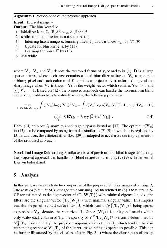
Algorithm 1 Pseudo-code of the propose approach

Input: Blurred image yOutput: The blur kernel k

1: Initialize: k,x,Jj ,B, δ2, γj,c, λ, β and d2: while stopping criterion is not satisfied do

3: Inferring latent image x, learning filters Jj and variances γj,c by (7)-(9)

4: Update for blur kernel k by (11)

5: Learning for noise δ2 by (10)

6: end while

where Vy, Vx and Vn denote the vectored forms of y, x and n in (1). D is a large

sparse matrix, where each row contains a local blur filter acting on Vx to generate

a blurry pixel and each column of E contains a projectively transformed copy of the

sharp image when Vx is known. Vk is the weight vector which satisfies Vkt ≥ 0 and∑t Vkt = 1. Based on (12), the proposed approach can handle the non-uniform blind

deblurring problem by alternatively solving the following problems:

maxq(Vx),D,Jj ,γj,c

∫q(Vx) log q(Vx)dVx −

∫q(Vx) log p(Vx,Vy|D,Jj , γj,c)dVx, (13)

minVk

‖∇EVk −V∇y‖22 + β‖Vk‖1. (14)

Here, (14) employs l1-norm to encourage a sparse kernel as [37]. The optimal q(Vx)in (13) can be computed by using formulas similar to (7)-(9) in which k is replaced by

D. In addition, the efficient filter flow [39] is adopted to accelerate the implementation

of the proposed approach.

Non-blind Image Deblurring Similar as most of previous non-blind image deblurring,

the proposed approach can handle non-blind image deblurring by (7)-(9) with the kernel

k given beforehand.

5 Analysis

In this part, we demonstrate two properties of the proposed SGF in image deblurring. 1)

The learned filters in SGF are sparse-promoting. As mentioned in (8), the filters in S-

GF are estimated as the eigenvector of 〈TxWjTTx 〉 with minimal eigenvalue, viz., the

filters are the singular vector 〈Tx(Wj)1

2 〉 with minimal singular value. This implies

that the proposed method seeks filters Jj which lead to VTJjTx(Wj)

1

2 being sparse

as possible. VJjdenotes the vectorized Jj . Since (Wj)

1

2 is a diagonal matrix which

only scales each column of Tx, the sparsity of VTJjTx(Wj)

1

2 is mainly determined by

VTJjTx. Consequently, the proposed approach seeks filters Jj which lead to the cor-

responding response VJjTx of the latent image being as sparse as possible. This can

be further illustrated by the visual results in Fig. 3(a) where the distribution of image


-1 0 1

log2

pro

babi

lity

dens

ity-20

-15

-10

-5

0

Output in our adaptive filter spacesOutput in the gradient spaces

-0.2 0 0.2-20

-15

-10

-5

0

-0.2 0 0.2-20

-15

-10

-5

0

-0.2 0 0.2

log2

pro

babi

lity

dens

ity

-20

-15

-10

-5

0

-0.1 0 0.1-20

-15

-10

-5

0

The corresponding filters

(a) Output (b) Results

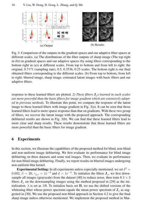
Fig. 3: Comparison of the outputs in the gradient spaces and our adaptive filter spaces at

different scales. (a) The distributions of the filter outputs of sharp image (The top right

in (b)) in gradient spaces and our adaptive spaces (by using filters corresponding to the

bottom right in (a)) at different scales. From top to bottom and from left to right: the

original, 0.7171 (sampling rate), 0.5, 0.3536, 0.25 scales. The bottom right is our final

obtained filters corresponding to the different scales. (b) From top to bottom, from left

to right: blurred image, sharp image, estimated latent images with basic filters and our

adaptive filters.

response to these learned filters are plotted. 2) These filters Jjs learned in each scales

are more powerful than the basic filters for image gradient which are extensively adopt-

ed in previous methods. To illustrate this point, we compare the response of the latent

image to these learned filters with image gradient in Fig. 3(a). It can be seen that those

learned filters lead to more sparse response than that on gradients. With these two group

of filters, we recover the latent image with the proposed approach. The corresponding

deblurred results are shown in Fig. 3(b). We can find that these learned filters lead to

more clear and sharp results. These results demonstrate that those learned filters are

more powerful than the basic filters for image gradient.

6 Experiments

In this section, we illustrate the capabilities of the proposed method for blind, non-blind

and non-uniform image deblurring. We first evaluate its performance for blind image

deblurring on three datasets and some real images. Then, we evaluate its performance

for non-blind image deblurring. Finally, we report results on blurred images undergoing

non-uniform blur kernel.

Experimental Setting: In all experiments unless especially mentioned, we set δ2 =0.002, β = 20, γj,c = 1e−3 and d = 1e−4. To initialize the filters Jj , we first down-

sample all images (grayscale) from the dataset [40] to reduce noise, then train 8 3 × 3filters Jj on the downsampling images using the method proposed in [29] as the ini-

tialization. λ is set as 1/8. To initialize basis set B, we use the shifted versions of the

whitening filter whose power spectrum equals the mean power spectrum of Jj as sug-

gested in [30]. We use the proposed non-blind approach in Section 4.2 to give the final

sharp image unless otherwise mentioned. We implement the proposed method in Mat-


Error ratios1.5 2 2.5 3 3.5 4

Su

cce

ss p

erce

nt

0.2

0.4

0.6

0.8

1

Ours

Babacan et al.

Levin et al.

Krishnan et al.

Xu et al.

Xu and Jia

Cho and Lee

Fergus et al.

Sun et al.

GSM-FoE

Ours w/o updating filters

Yan et al.

Pan et al.

(a)

Error ratios1 2 3 4 5

Suc

cess

per

cent

0

0.2

0.4

0.6

0.8

1

OursPan et al.Yan et al.Levin et al.Krishnan et al.Xu and JiaCho and LeeMichaeli and IraniSun et al.

(b)

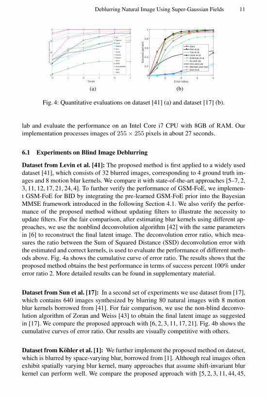
Fig. 4: Quantitative evaluations on dataset [41] (a) and dataset [17] (b).

lab and evaluate the performance on an Intel Core i7 CPU with 8GB of RAM. Our

implementation processes images of 255× 255 pixels in about 27 seconds.

6.1 Experiments on Blind Image Deblurring

Dataset from Levin et al. [41]: The proposed method is first applied to a widely used

dataset [41], which consists of 32 blurred images, corresponding to 4 ground truth im-

ages and 8 motion blur kernels. We compare it with state-of-the-art approaches [5–7, 2,

3, 11, 12, 17, 21, 24, 4]. To further verify the performance of GSM-FoE, we implemen-

t GSM-FoE for BID by integrating the pre-learned GSM-FoE prior into the Bayesian

MMSE framework introduced in the following Section 4.1. We also verify the perfor-

mance of the proposed method without updating filters to illustrate the necessity to

update filters. For the fair comparison, after estimating blur kernels using different ap-

proaches, we use the nonblind deconvolution algorithm [42] with the same parameters

in [6] to reconstruct the final latent image. The deconvolution error ratio, which mea-

sures the ratio between the Sum of Squared Distance (SSD) deconvolution error with

the estimated and correct kernels, is used to evaluate the performance of different meth-

ods above. Fig. 4a shows the cumulative curve of error ratio. The results shows that the

proposed method obtains the best performance in terms of success percent 100% under

error ratio 2. More detailed results can be found in supplementary material.

Dataset from Sun et al. [17]: In a second set of experiments we use dataset from [17],

which contains 640 images synthesized by blurring 80 natural images with 8 motion

blur kernels borrowed from [41]. For fair comparison, we use the non-blind deconvo-

lution algorithm of Zoran and Weiss [43] to obtain the final latent image as suggested

in [17]. We compare the proposed approach with [6, 2, 3, 11, 17, 21]. Fig. 4b shows the

cumulative curves of error ratio. Our results are visually competitive with others.

Dataset from Kohler et al. [1]: We further implement the proposed method on dateset,

which is blurred by space-varying blur, borrowed from [1]. Although real images often

exhibit spatially varying blur kernel, many approaches that assume shift-invariant blur

kernel can perform well. We compare the proposed approach with [5, 2, 3, 11, 44, 45,


Image1 Image2 Image3 Image4 Average

PS

NR

0

5

10

15

20

25

30

35

BlurredCho and LeeXu and JiaShan et al.Fergus et al.Krishnan et al.Whyte et al.Hirsch et al.Pan et al.Yan et al.Ours

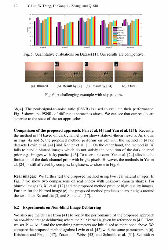
Fig. 5: Quantitative evaluations on Dataset [1]. Our results are competitive.

(a) Blurred (b) Result by [4] (c) Result by [24] (d) Ours

Fig. 6: A challenging example with sky patches.

38, 4]. The peak-signal-to-noise ratio (PSNR) is used to evaluate their performance.

Fig. 5 shows the PSNRs of different approaches above. We can see that our results are

superior to the state-of-the-art approaches.

Comparison of the proposed approach, Pan et al. [4] and Yan et al. [24]: Recently,

the method in [4] based on dark channel prior shows state-of-the-art results. As shown

in Figs. 4a and 5, the proposed method performs on par with the method in [4] on

datasets Levin et al. [41] and Kohler et al. [1]. On the other hand, the method in [4]

fails to handle blurred images which do not satisfy the condition of the dark channel

prior, e.g., images with sky patches [46]. To a certain extent, Yan et al. [24] alleviate the

limitation of the dark channel prior with bright pixels. However, the methods in Yan et

al. [24] is still affected by complex brightness, as shown in Fig. 6.

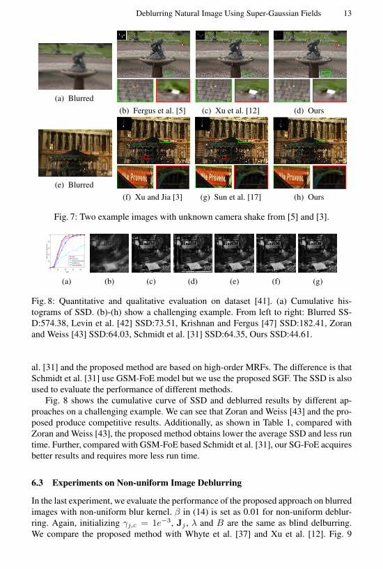
Real images: We further test the proposed method using two real natural images. In

Fig. 7 we show two comparisons on real photos with unknown camera shakes. For

blurred image (a), Xu et al. [12] and the proposed method produce high-quality images.

Further, for the blurred image (e), the proposed method produces sharper edges around

the texts than Xu and Jia [3] and Sun et al. [17].

6.2 Experiments on Non-blind Image Deblurring

We also use the dataset from [41] to verify the performance of the proposed approach

on non-blind image deblurring where the blur kernel is given by reference to [41]. Here,

we set δ2 = 1e−4 and the remaining parameters are initialized as mentioned above. We

compare the proposed method against Levin et al. [42] with the same parameters in [6],

Krishnan and Fergus [47], Zoran and Weiss [43] and Schmidt et al. [31]. Schmidt et


(a) Blurred

(b) Fergus et al. [5] (c) Xu et al. [12] (d) Ours

(e) Blurred

(f) Xu and Jia [3] (g) Sun et al. [17] (h) Ours

Fig. 7: Two example images with unknown camera shake from [5] and [3].

SSD0 20 40 60 80

Su

cce

ss p

erc

en

t

0

0.2

0.4

0.6

0.8

1

OursLevin et al.Krishnan and FergusSchmidt et al.Zoran and Weiss

(a) (b) (c) (d) (e) (f) (g)

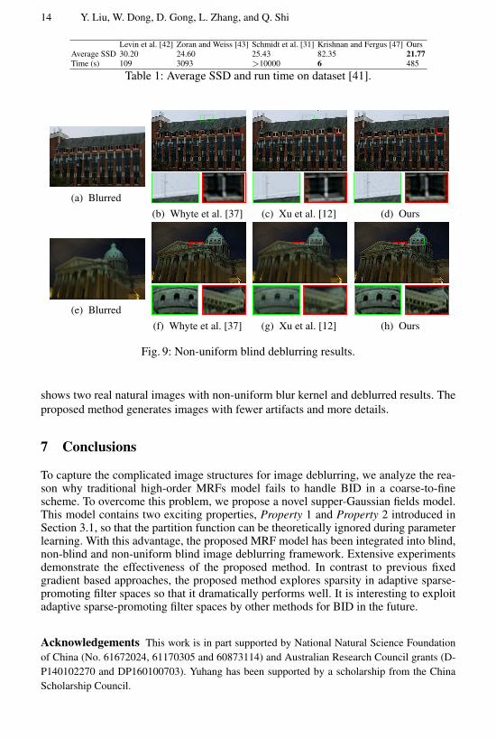
Fig. 8: Quantitative and qualitative evaluation on dataset [41]. (a) Cumulative his-

tograms of SSD. (b)-(h) show a challenging example. From left to right: Blurred SS-

D:574.38, Levin et al. [42] SSD:73.51, Krishnan and Fergus [47] SSD:182.41, Zoran

and Weiss [43] SSD:64.03, Schmidt et al. [31] SSD:64.35, Ours SSD:44.61.

al. [31] and the proposed method are based on high-order MRFs. The difference is that

Schmidt et al. [31] use GSM-FoE model but we use the proposed SGF. The SSD is also

used to evaluate the performance of different methods.

Fig. 8 shows the cumulative curve of SSD and deblurred results by different ap-

proaches on a challenging example. We can see that Zoran and Weiss [43] and the pro-

posed produce competitive results. Additionally, as shown in Table 1, compared with

Zoran and Weiss [43], the proposed method obtains lower the average SSD and less run

time. Further, compared with GSM-FoE based Schmidt et al. [31], our SG-FoE acquires

better results and requires more less run time.

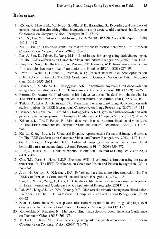
6.3 Experiments on Non-uniform Image Deblurring

In the last experiment, we evaluate the performance of the proposed approach on blurred

images with non-uniform blur kernel. β in (14) is set as 0.01 for non-uniform deblur-

ring. Again, initializing γj,c = 1e−3, Jj , λ and B are the same as blind delburring.

We compare the proposed method with Whyte et al. [37] and Xu et al. [12]. Fig. 9


Levin et al. [42] Zoran and Weiss [43] Schmidt et al. [31] Krishnan and Fergus [47] Ours

Average SSD 30.20 24.60 25.43 82.35 21.77

Time (s) 109 3093 >10000 6 485

Table 1: Average SSD and run time on dataset [41].

(a) Blurred

(b) Whyte et al. [37] (c) Xu et al. [12] (d) Ours

(e) Blurred

(f) Whyte et al. [37] (g) Xu et al. [12] (h) Ours

Fig. 9: Non-uniform blind deblurring results.

shows two real natural images with non-uniform blur kernel and deblurred results. The

proposed method generates images with fewer artifacts and more details.

7 Conclusions

To capture the complicated image structures for image deblurring, we analyze the rea-son why traditional high-order MRFs model fails to handle BID in a coarse-to-finescheme. To overcome this problem, we propose a novel supper-Gaussian fields model.This model contains two exciting properties, Property 1 and Property 2 introduced inSection 3.1, so that the partition function can be theoretically ignored during parameterlearning. With this advantage, the proposed MRF model has been integrated into blind,non-blind and non-uniform blind image deblurring framework. Extensive experimentsdemonstrate the effectiveness of the proposed method. In contrast to previous fixedgradient based approaches, the proposed method explores sparsity in adaptive sparse-promoting filter spaces so that it dramatically performs well. It is interesting to exploitadaptive sparse-promoting filter spaces by other methods for BID in the future.

Acknowledgements This work is in part supported by National Natural Science Foundation

of China (No. 61672024, 61170305 and 60873114) and Australian Research Council grants (D-

P140102270 and DP160100703). Yuhang has been supported by a scholarship from the China

Scholarship Council.


References

1. Kohler, R., Hirsch, M., Mohler, B., Scholkopf, B., Harmeling, S.: Recording and playback of

camera shake: Benchmarking blind deconvolution with a real-world database. In: European

Conference on Computer Vision. Springer (2012) 27–40

2. Cho, S., Lee, S.: Fast motion deblurring. In: ACM SIGGRAPH Asia 2009 Papers. (2009)

145:1–145:8

3. Xu, L., Jia, J.: Two-phase kernel estimation for robust motion deblurring. In: European

Conference on Computer Vision. (2010) 157–170

4. Pan, J., Sun, D., Pfister, H., Yang, M.H.: Blind image deblurring using dark channel prior.

In: The IEEE Conference on Computer Vision and Pattern Recognition. (2016) 1628–1636

5. Fergus, R., Singh, B., Hertzmann, A., Roweis, S.T., Freeman, W.T.: Removing camera shake

from a single photograph. Acm Transactions on Graphics 25(25) (2006) 787–794

6. Levin, A., Weiss, Y., Durand, F., Freeman, W.T.: Efficient marginal likelihood optimization

in blind deconvolution. In: The IEEE Conference on Computer Vision and Pattern Recogni-

tion. (2011) 2657–2664

7. Babacan, S.D., Molina, R., Katsaggelos, A.K.: Variational bayesian blind deconvolution

using a total variation prior. IEEE Transactions on Image processing 18(1) (2009) 12–26

8. Perrone, D., Favaro, P.: Total variation blind deconvolution: The devil is in the details. In:

The IEEE Conference on Computer Vision and Pattern Recognition. (2014) 2909–2916

9. Tzikas, D., Likas, A., Galatsanos, N.: Variational bayesian blind image deconvolution with

student-t priors. In: IEEE International Conference on Image Processing. (2007) 109–112

10. Babacan, S.D., Molina, R., Do, M.N., Katsaggelos, A.K.: Bayesian blind deconvolution with

general sparse image priors. In: European Conference on Computer Vision. (2012) 341–355

11. Krishnan, D., Tay, T., Fergus, R.: Blind deconvolution using a normalized sparsity measure.

In: The IEEE Conference on Computer Vision and Pattern Recognition, IEEE (2011) 233–

240

12. Xu, L., Zheng, S., Jia, J.: Unnatural l0 sparse representation for natural image deblurring.


13. Ge, D., Idier, J., Carpentier, E.L.: Enhanced sampling schemes for mcmc based blind

bernoulli gaussian deconvolution. Signal Processing 91(4) (2009) 759–772

14. Roth, S., Black, M.J.: Fields of experts. International Journal of Computer Vision 82(2)

(2009) 205

15. Cho, T.S., Paris, S., Horn, B.K.P., Freeman, W.T.: Blur kernel estimation using the radon

transform. In: The IEEE Conference on Computer Vision and Pattern Recognition. (2011)

241–248

16. Joshi, N., Szeliski, R., Kriegman, D.J.: Psf estimation using sharp edge prediction. In: The

IEEE Conference on Computer Vision and Pattern Recognition. (2008) 1–8

17. Sun, L., Cho, S., Wang, J., Hays, J.: Edge-based blur kernel estimation using patch priors.

In: IEEE International Conference on Computational Photography. (2013) 1–8

18. Lai, W.S., Ding, J.J., Lin, Y.Y., Chuang, Y.Y.: Blur kernel estimation using normalized color-

line priors. In: The IEEE Conference on Computer Vision and Pattern Recognition. (2015)

64–72

19. Zhou, Y., Komodakis, N.: A map-estimation framework for blind deblurring using high-level

edge priors. In: European Conference on Computer Vision. (2014) 142–157

20. Komodakis, N., Paragios, N.: Mrf-based blind image deconvolution. In: Asian Conference

on Computer Vision. (2013) 361–374

21. Michaeli, T., Irani, M.: Blind deblurring using internal patch recurrence. In: European

Conference on Computer Vision. (2014) 783–798


22. Gong, D., Tan, M., Zhang, Y., Hengel, A.V.D., Shi, Q.: Blind image deconvolution by auto-

matic gradient activation. In: The IEEE Conference on Computer Vision and Pattern Recog-

nition. (2016) 1827–1836

23. Gong, D., Tan, M., Zhang, Y., van den Hengel, A., Shi, Q.: Self-paced kernel estimation

for robust blind image deblurring. In: International Conference on Computer Vision. (2017)

1661–1670

24. Yan, Y., Ren, W., Guo, Y., Wang, R., Cao, X.: Image deblurring via extreme channels prior.


25. Nimisha, T., Singh, A.K., Rajagopalan, A.: Blur-invariant deep learning for blind-deblurring.

In: The IEEE International Conference on Computer Vision. Volume 2. (2017)

26. Xu, X., Pan, J., Zhang, Y.J., Yang, M.H.: Motion blur kernel estimation via deep learning.

IEEE Transactions on Image Processing 27(1) (2018) 194–205

27. Zhang, L., Wei, W., Zhang, Y., Shen, C., van den Hengel, A., Shi, Q.: Cluster sparsity

field: An internal hyperspectral imagery prior for reconstruction. International Journal of

Computer Vision (2018) 1–25

28. Besag, J.: Spatial interaction and the statistical analysis of lattice systems. Journal of the

Royal Statistical Society. Series B (Methodological) (1974) 192–236

29. Schmidt, U., Gao, Q., Roth, S.: A generative perspective on mrfs in low-level vision. In: The

IEEE Conference on Computer Vision and Pattern Recognition. (2010) 1751–1758

30. Weiss, Y., Freeman, W.T.: What makes a good model of natural images? In: The IEEE

Conference on Computer Vision and Pattern Recognition. (2007) 1–8

31. Schmidt, U., Schelten, K., Roth, S.: Bayesian deblurring with integrated noise estimation.


32. Zhang, H., Zhang, Y., Li, H., Huang, T.S.: Generative bayesian image super resolution with

natural image prior. IEEE Transactions on Image processing 21(9) (2012) 4054–4067

33. Palmer, J.A., Wipf, D.P., Kreutz-Delgado, K., Rao, B.D.: Variational em algorithms for non-

gaussian latent variable models. In: Advances in Neural Information Processing Systems.

(2005) 1059–1066

34. Levin, A., Weiss, Y., Durand, F., Freeman, W.T.: Understanding blind deconvolution algo-

rithms. IEEE transactions on pattern analysis and machine intelligence 33(12) (2011) 2354

35. Murphy, K.P.: Machine learning: a probabilistic perspective. MIT Press, Cambridge, MA

(2012)

36. Wipf, D., Zhang, H.: Revisiting bayesian blind deconvolution. The Journal of Machine

Learning Research 15(1) (2014) 3595–3634

37. Whyte, O., Sivic, J., Zisserman, A., Ponce, J.: Non-uniform deblurring for shaken images.

International journal of computer vision 98(2) (2012) 168–186

38. Hirsch, M., Schuler, C.J., Harmeling, S., Scholkopf, B.: Fast removal of non-uniform camera

shake. In: International Conference on Computer Vision. (2011) 463–470

39. Hirsch, M., Sra, S., Scholkopf, B., Harmeling, S.: Efficient filter flow for space-variant

multiframe blind deconvolution. In: The IEEE Conference on Computer Vision and Pattern

Recognition. (2010) 607–614

40. Martin, D.R., Fowlkes, C., Tal, D., Malik, J.: A database of human segmented natural images

and its application to. Proc.intl Conf.computer Vision 2(11) (2002) 416–423 vol.2

41. Levin, A., Weiss, Y., Durand, F., Freeman, W.T.: Understanding and evaluating blind decon-

volution algorithms. In: The IEEE Conference on Computer Vision and Pattern Recognition.

(2009) 1964–1971

42. Levin, A., Fergus, R., Durand, F., Freeman, W.T.: Image and depth from a conventional

camera with a coded aperture. Acm Transactions on Graphics 26(3) (2007) 70

43. Zoran, D., Weiss, Y.: From learning models of natural image patches to whole image restora-

tion. In: IEEE International Conference on Computer Vision. (2011) 479–486


44. Shan, Q., Jia, J., Agarwala, A.: High-quality motion deblurring from a single image. Acm

Transactions on Graphics 27(3) (2008) 15–19

45. Whyte, O., Sivic, J., Zisserman, A.: Deblurring shaken and partially saturated images. Inter-

national Journal of Computer Vision 110(2) (2014) 185–201

46. He, K., Sun, J., Tang, X.: Single image haze removal using dark channel prior. IEEE trans-

actions on pattern analysis and machine intelligence 33(12) (2011) 2341–2353

47. Krishnan, D., Fergus, R.: Fast image deconvolution using hyper-laplacian priors. In: Ad-

vances in Neural Information Processing Systems. (2009) 1033–1041

deblurring natural image using super-gaussian fieldsopenaccess.thecvf.com › ... ›...

Documents