ISSN 2385-2755 Working papers

(Dipartimento di scienze sociali ed economiche) [online]

SAPIENZA – UNIVERSITY OF ROME P.le Aldo Moro n.5 – 00185 Roma T (+39) 06 49910563 F (+39) 06 49910231 CF 80209930587 - P.IVA 02133771002

WORKING PAPERS SERIES

DIPARTIMENTO DI

SCIENZE SOCIALI ED ECONOMICHE

n. 9/2016

Debt Overhang and Sovereign Debt Restructuring

Author/s:

Mattia Osvaldo Picarelli

Debt Overhang and Sovereign Debt Restructuring∗

Mattia Osvaldo Picarelli

Sapienza University of Rome

November 21, 2016

Abstract

Debt overhang is dened as a situation where a large amount of debt distorts the

optimal investment decisions and discourages the government's eorts of the debtor

country to undertake the necessary "adjustment policies".

In this paper I study some dierent strategies that can be used to solve the sovereign

debt overhang problem. In particular, I consider two strategies based on a debt re-

structuring process, via haircut or rescheduling, and a third one based on conditional-

additional lending. This strategy relies on the idea that the debtor country can get

new lending from the existing creditors, in order to undertake investments that can

aect the productivity shock distribution in a positive way (or reduce the probability

of default).

The aim of this paper is to study the consequences, deriving from the three strategies

described, on the incentives to invest in a "troubled country". According to these con-

sequences and under some specic conditions, I rank the three strategies in order to see

which is the most eective one. In particular, I nd that if the change in investments

due to the conditional-additional lending makes the probability of default low in this

scenario, the conditional lending strategy will be the most eective one. Basically, this

paper might help the policy-makers to implement the right intervention according to

the specic scenarios considered.

JEL Codes: C78, F34, H63

Keywords: Debt Overhang, Debt Restructuring, Nash Bargaining, Haircut,

Rescheduling, Conditional Lending.

∗I would like to thank Nicola Borri, Salvatore Nisticó, Dario Briscolini and all members of the board of

PhD programme in Economics and Finance for their useful comments and suggestions. The research was

developed within the framework of the PhD programme in Economics and Finance of Sapienza University.

1

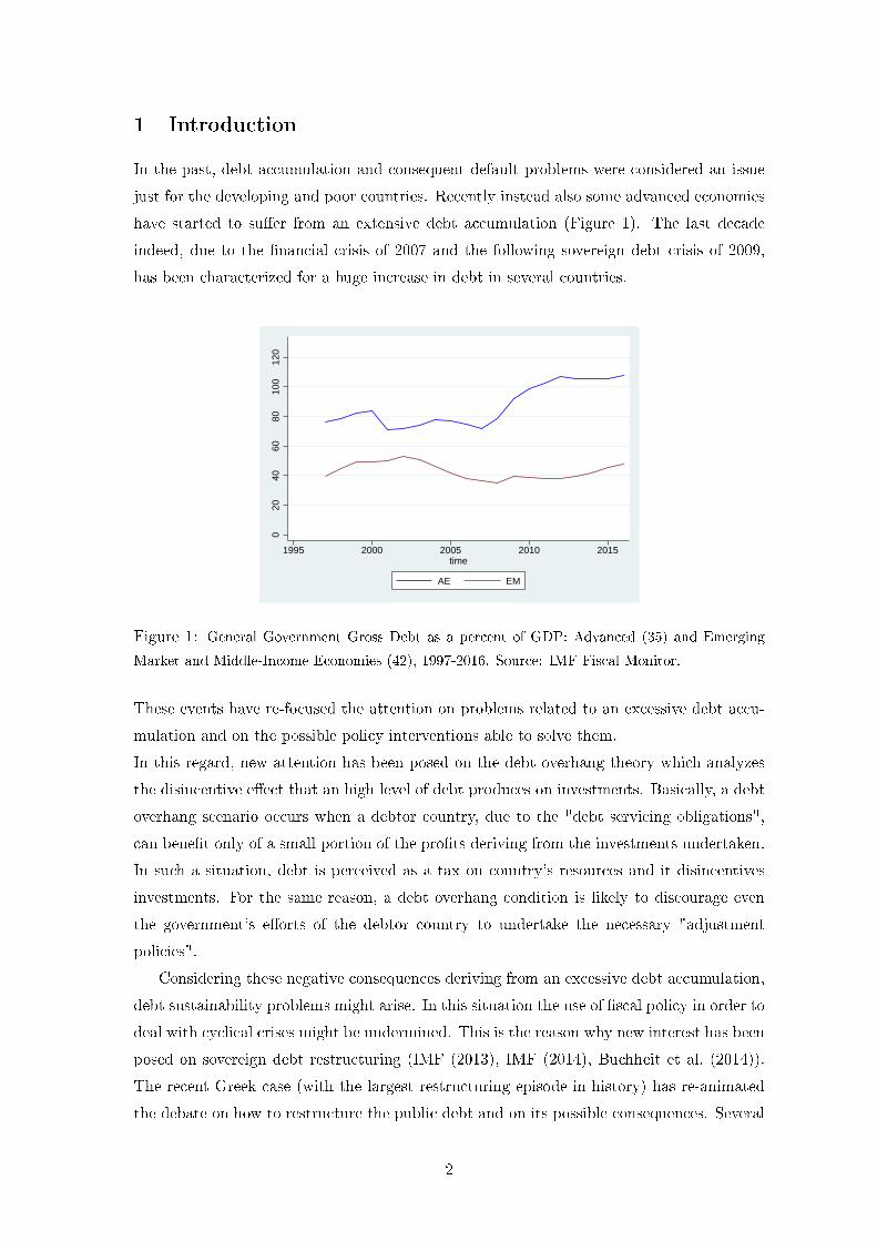
1 Introduction

In the past, debt accumulation and consequent default problems were considered an issue

just for the developing and poor countries. Recently instead also some advanced economies

have started to suer from an extensive debt accumulation (Figure 1). The last decade

indeed, due to the nancial crisis of 2007 and the following sovereign debt crisis of 2009,

has been characterized for a huge increase in debt in several countries.0

2040

6080

100

120

1995 2000 2005 2010 2015time

AE EM

Figure 1: General Government Gross Debt as a percent of GDP: Advanced (35) and Emerging

Market and Middle-Income Economies (42), 1997-2016. Source: IMF Fiscal Monitor.

These events have re-focused the attention on problems related to an excessive debt accu-

mulation and on the possible policy interventions able to solve them.

In this regard, new attention has been posed on the debt overhang theory which analyzes

the disincentive eect that an high level of debt produces on investments. Basically, a debt

overhang scenario occurs when a debtor country, due to the "debt servicing obligations",

can benet only of a small portion of the prots deriving from the investments undertaken.

In such a situation, debt is perceived as a tax on country's resources and it disincentives

investments. For the same reason, a debt overhang condition is likely to discourage even

the government's eorts of the debtor country to undertake the necessary "adjustment

policies".

Considering these negative consequences deriving from an excessive debt accumulation,

debt sustainability problems might arise. In this situation the use of scal policy in order to

deal with cyclical crises might be undermined. This is the reason why new interest has been

posed on sovereign debt restructuring (IMF (2013), IMF (2014), Buchheit et al. (2014)).

The recent Greek case (with the largest restructuring episode in history) has re-animated

the debate on how to restructure the public debt and on its possible consequences. Several

2

proposal for a dierent form of debt restructuring have been advanced in the last years

(Gianviti et al (2010), Paris and Wyplosz (2014)).

The aim of this paper is to build a two periods model with default risk that allows to

analyze the eects of three dierent strategies, able to solve a debt overhang problem and

to restore the incentives to invest in a highly indebted country, in order to nd out the

most eective one:

1. Sovereign debt restructuring: haircut

2. Sovereign debt restructuring: lenghtening of maturities

3. Conditional lending

With a large amount of outstanding debt, maintaining unchanged the nominal value of

the debtor's obligations can produce negative consequences for both creditors and debtor.

In such a situation and according to the debt overhang theory, a debt reduction could be

an ecient strategy for both creditors and debtor countries. It should restore incentives to

invest although it is not known which might be the most eective way to do that: haircut

or lengthening maturities. A priori, it would seem reasonable to assume that an haircut

can produce more eective results as it would deal with debt problems once and for all,

solving denitely the problem of uncertainty. A lengthening of maturities process instead

may just exacerbate the debt overhang condition by postponing the solution of the problem

and without eliminating the uncertainty related to the borrower's nancial conditions and

repayment capacity.

The third strategy here analyzed is the so called "conditional lending" that is based on an

additional nancing, from existing lenders, for the debtor country. These creditors may,

indeed, grant additional loans with the aim to protect the value of their claims toward the

debtor country.

Just to give an example, after the eruption of the sovereign debt crisis and the provision of

some additional lendings for Greece, debt restucturing interventions in the form of haircut

became necessary in order to recover from a dramatic situation and to calm down the

markets. This means that the strategy of providing new lending to the debtor country

might work just under some specic conditions. I assume such new lending "conditional"

because it is related to the debtor's commitment to make the necessary "adjustments"

(investments). Moreover, I assume this new lending constrained by a specic credit ceiling

and able to reduce the probability of default under specic conditions.

A comparison between these three strategies, with a focus on their consequences, might

be useful in order to see which is the best way to deal with a debt overhang problem. In

particular, given the current Greek crisis, such study might provide some useful information

for the policy makers who are trying to solve the situation.

3

The paper proceeds as follows: Section 2 makes a literature review; Section 3 develops

the theoretical model characterizing the restructuring through haircut, the restructuring

through rescheduling and the conditional lending strategy; Section 4 concludes.

2 Related Literature

The debt overhang theory has been introduced for the rst time by Myers (1977) in a

corporate context. He dened debt overhang as a situation where the high level of debt

distorts the possibilities for companies to make optimal future investment decisions. More

specically, a rm is less incentivated to invest because the benets (i.e. future cash ows)

deriving from the additional investment undertaken must be used largely to reimbourse

the existing debt holders (rather than to pay the shareholders). The larger is the prot

that goes to the creditors the lower is the incentive to invest and to suer the cost of

investment for the shareholders. Potential lenders might even decide to not nance the

rm because of its high debt. Otherwise, they might ask for an higher interest rate in order

to protect themselves. This reduces debtor's gain deriving from the investment undertaken

thus creating a disincentive eect in the rm's investments policy. This reduced incentive

to invest may then imply an underinvestment problem for rms with high levels of debt.

An example might be useful to clarify the debt overhang concept. Let's consider a rm

with a debt of $100, due the next year, and a future income of $80 (i.e. the company

will be in default the next year). Let's assume there is an investment opportunity that

costs $5 and produces $15 next year 1 and the rm needs to raise funds to nance it. If

the existing creditors are senior, then there will be no new investors willing to nance the

project because the benets will go just to the original creditors (who will increase their

payo to $95) whereas the new ones will get nothing. If, instead, the project gives $30 the

next year, new investors might be interested in funding the project because they can get

$10 next year in return for the $5 invested today. In conclusion, it is possible to nance

investment just if the NPV of investing is larger than the debt overhang (here dened as

the dierence between assets and liabilities).

This concept of debt overhang used in the nance literature is similar to the concept used

in the macro literature where the debt overhang has been analyzed mainly in the context of

sovereign-debt crises. Indeed, due to the debt crises in the 80s and 90s, this theory has been

extended in a sovereign context with the aim to explain the eects that the high debt had

produced on the level of investment in the "less developed countries" (LDCs)2. In those

1assume the interest rate is zero so the project has a NPV of $10.2Several papers have analyzed these eects in that period (Krugman (1988), Krugman (1989), Boren-

sztein (1990), Obstfeld and Rogo (1996) and Sachs (1989)).

4

years, the highly indebted countries' low investments level and the low growth rate were

often attributed, at least in part, to the high level of foreign debt. According to the debt

overhang assumption, the accumulated debt discourages private sector's investment and the

government's adjustment eorts because a possible improvement in the debtor country's

performances determines mainly an increase in creditors' repayment.

From an empirical point of view, several studies tried to quantify the negative eects

produced by an high level of debt. From on side, the literature focused on the eects on

investments (Deshpande (1997)); from the other side, it focused on the direct eect on

GDP growth rate. In this regard, some papers identied a non-linear relationship between

debt and growth (Pattillo et al (2011); Clements et al (2003) and Reinhart et al (2012))

showing that high debt can aect negatively growth just if some thresholds are reached.

Several papers showed how desirable a debt relief was in the 80s and 90s for the LDCs.

The debate was focused on the eects produced by the implemented restructuring programs.

In particular, part of the literature showed the benecial eects that some debt restructuring

plans (the Brady Plan over all) produced in some countries. Arslanalp and Henry (2004)

show the positive consequences that the Brady Plan had for both creditor and debtors

countries. Specically, they analyze these positive eects with respect to the stock prices

for the debtor countries involved and the US commercial banks (i.e. the largest creditors

at that time) with signicant loan exposure towards those countries.

See Arslanalp and Henry (2006) for a literature review on the debt overhang problem.

In order to study the dierent possibilities available to restructure sovereign debt, it is

useful to start from the survey of Das et al (2012a) and Das et al (2012b). In these papers,

some interesting "stlylized facts" are described such as the frequency of restructuring, the

number of London and Paris Club deals, the procedures used etc. regarding the several

restructuring episodes that occurred between 1950 and 2010. In particular, some dierences

between the restructuring processes implemented by haircut and processes implemented by

lengthening maturities are highlighted.

Even Reinhart and Trebesch (2015) analyze, but just from an empirical point of view,

the dierent consequences produced by restructuring processes implemented via haircut or

via lengthening maturities. In particular, they show that the debtor countries' conditions

(economic growth or credit ratings) improve signicantly just in case of debt write-os.

Dierent form of debt reliefs instead, such as lenghtening of maturities, are not generally

followed by such results.

Let's see now how the three strategies, described in the introduction, have been treated

so far.

In literature, a debt restructuring via haircut was initially analyzed by considering an

exogenous debt reduction. Examples are given by Marchesi and Thomas (1999), Froot

(1989) and Sachs (1989).

5

Literature has just recently started to consider an endogenous debt reduction, determined

in a renegotiation process between creditors and debtor country. In this regard, Yue (2010)

and Prokop (2012) are interesting papers because they consider a renegotiation between

creditors and debtor in the form of a Nash Bargaining.

To my knowledge, no theoretical model has been built to study the eects, in a debt

overhang context, of a debt restructuring via lengthening of maturities. However, the

three periods model presented in Fernandez and Martin (2015) oers interesting food for

thought for my goal especially in term of rollover risk. Bac (1999) instead considers an

extreme lenghtening of maturity in the form of grace periods deriving as a Nash equilibrium

creditors' strategy in a dynamic non cooperative game.

Finally, regarding the conditional lending (analyzed in particular by Obstfeld and Rogo

(1996), Sachs and Cohen (1982) and Krugman (1988)), most of the literature has argued

that the strategy of granting new loans to an indebted country appears to be eective.

Several studies have shown indeed that the liquidity constraints of debtor countries were just

the main reason of low investment (Sachs and Cohen (1982), Froot (1989) and Borensztein

(1988)). This may suggest that debt reduction operations should be accompanied by further

loans in order to be more eective.

3 The Model

Let's consider a two periods model (t = 1, 2) for a debtor country that can be described by

the following timeline:

At time t = 1 the country has an exogenous endowment Y1 and an investment opportunity.

The country then invests K2 at t = 1 and gets a prot AF (K2) at time 2 (capital is

assumed to depreciate at 100 %) with F ′′(K2) < 0. ”A” is the productivity shock and it

is represented by a random variable that belongs to [A, A], with E(A) = 1 and density

probability function π(A).

It is further assumed that the country has inherited debt D that expires in t = 2. It means

that AF (K2) will be used in t = 2 for both consumption and debt repayment.

Let's assume that the country is risk neutral with the following utility function:

U1 = C1 + E(C2) (1)

To simplify, it is assumed that the discount factor is β = 1 and that the world interest rate

6

is r = 0.

Moreover, I assume that ηAF (K2) represents the output reduction for the debtor country

in case of default (as a deadweight loss) 3 with 0 < η < 1.

At time t = 1, consumption is given by C1 = Y1−K2 whereas in t = 2 by C2 = AF (K2)−P .P represents the debtor's payment P = min[D, ηAF (K2)] which depends on the realizations

of A. From this expression it is possible to identify two intervals for the realizations of the

variable A:

• if A < DηF (K2)

default will be more convenient for the debtor country as the output

reduction in case of default is less than the cost of debt repayment;

• if A > DηF (K2)

the country repays its debt because it is more convenient compared to

the loss of output that it would suer in case of default.

To see the eect on the debt overhang problem of an haircut restructuring process, I assume

that in case of default in t = 2, there is a re-negotiation between creditors and debtor in

the form of Nash Bargaining. In this re-negotiation, an haircut on debt is determined in

an endogenous way.

Let's see in more details how this re-negotiation process works.

3.1 Restructuring via haircut

In the Nash Bargaining there are two dierent scenarios that must be taken into account:

1. Agreement: the creditors receive as payment the new level of debt determined in

the re-negotiation process whereas the debtor gets the dierence between the output

produced in the second period and what it must repay:

UC = D(1− h)

UD = AF (K2)−D(1− h)

2. No Agreement: to simplify I assume that the creditors gets nothing whereas the

debtor suers a reduction in its output because of the default:

UC = 0

UD = (1− η)AF (K2)

3ηAF (K2) in literature can be considered both as a fraction of output of the debtor country that can

be expropriated from creditors or just as an output reduction due to the default. In this paper I will

consider it as an output reduction. Several papers study the consequent output reduction for a country

in default deriving from trade sanctions (Rose (2005)), exclusion from nancial markets (Cruces and C.

(2013)), reduced credit to the private sector (Arteta and G. (2008))etc. The so called "issue linkages". For

a review see Sandleris (2012)

7

where UC and UD represent respectively creditors' and debtor's utility functions in case of

agreement (UC and UD in case of no agreement).

Thus, it is possible to build the creditors' (UC − UC) and debtor's surplus functions (UD−UD) that represent the utility gains of creditors and debtor country in case of agreement

in the Nash Bargaining. The resulting Nash product Ω must be maximized with respect

to h (i.e. the amount of haircut) considering θ as creditors' bargaining power and (1 − θ)as debtor's bargaining power. This is a maximization problem with creditors' and debtor's

surplus functions as constraints.

maxK2

Ω

s. t. UC − UC ≥ 0

s. t. UD − UD ≥ 0

The result of this maximization is:

h = 1− θηAF (K2)

D(2)

Computations are showed in Appendix A.

Thus, the amount of debt reduced that must be paid at the end of the Nash Bargaining

process is:

D(1− h) = θηAF (K2)

If θ = 0, there will be a 100% haircut: the debtor pays 0.

If θ = 1, there will be a 0% haircut: the debtor pays ηAF (K2).

If 0 < θ < 1, then 0 < h < 1 and the debtor pays an amount 0 < D(1− h) < ηAF (K2).

In conclusion, as we can see from equation (2), it is possible to claim that:

• an increase in creditors' bargaining power reduces the level of h;

• an higher output reduction in case of default negatively inuences the level of h (as

a sort of disincentive to default);

• an higher D implies the necessity of an higher haircut.

Thanks to the result of the restructuring process just found, consumption in the second

period can be re-written as:

C2 =

CR2 = AF (K2)−D(1− h)

CN2 = AF (K2)−D

8

With CR2 consumption in case of restructuring and CN2 consumption in case of no default.

Maximizing the (1) with respect to K2 and taking into account the result deriving from

the Nash bargaining produces the following result:

F ′(K2)

[1− θη

∫ DηF (K2)

A

Aπ(A)dA− π(

D

ηF (K2)

)D2

ηF (K2)2(1− θ)

]= 1 (3)

Computations are showed in Appendix A1.

θη∫ DηF (K2)

A Aπ(A)dA represents how the marginal change in K2 aects the payment in case

of haircut (if there is a change in the amount to be paid) and π(

DηF (K2)

)D2

ηF (K2)2 (1 − θ)

represents the dierence between the repayment change in case of no haircut and in case

of haircut due to a change in K2 (that aects the default probability).

Thus, it is possible to claim that the nal result, in terms of incentives to invest, de-

pends on the value of the parameter θ: the lower the value of this parameter, the higher

will be the incentives to invest. This is because the smaller the θ, the greater will be the

value assumed by h. In other words, the eectiveness of the haircut result depends on the

creditors' bargaining power.

In order to see how the creditors' bargaining power (θ) aects the relation between debt

and investment it is useful to compute the implicit dierentiation of (3).

dK2

dD=

[θD

ηF (K2)2F′(K2)π

(D

ηF (K2)

)+ F ′(K2)(1− θ) D

ηF (K2)2

(π′(

DηF (K2)

)D

ηF (K2) + 2π(

DηF (K2)

))]U ′′(K2)

that is negative if U ′′(K2) < 0.

Computations are showed in Appendix A2.

3.2 Restructuring via rescheduling

A second strategy here analyzed is related to a restructuring process via lengthening of

maturities. In order to model a rescheduling process, I add an intermediate period where

the debtor country has an exogenous endowment Y2 and it is due a debt payment D2. The

following timeline describes the current situation:

It is assumed that the debtor country doesn't have the necessary resources to repay this

amount of debt (Y2 < D2). Therefore, its only available strategy is to default on t = 2 and

it would imply an output loss for the debtor country both in t = 2 and t = 3.

9

From creditors' point of view, it is surely preferable to avoid a default as it would involve

a total loss of their claims. Thus, creditors give the opportunity to restructure the debt

through a lengthening of maturities. It means to postpone the payment of D2 from t = 2

to t = 3 through a debt rollover. Then, in the third period, since the debtor country gets

prots from investment and there is the realization of the productivity shock, creditors

might be fully repaid.

Since I am introducing the debt rollover's interest rate, it is necessary to consider a risk

free interest rate rF 6= 0 and a risky interest rate as a convex function of the level of debt

r = r(D). Thus, I assume that the debt is rolled over at the rate 1 + r. The interest rate

1 + r, dened in such a way, reects the riskiness of the debtor. If the debtor country has

a low level of debt, then the rollover implies a lower interest rate. Vice versa debt is rolled

over at an higher interest rate (because of the higher risk).

Thus, in t = 3 the debtor will pay the min[D∗, ηAF (K2)] with D∗ = D + D2(1 + r) that

represents the total debt that must be paid.

If A < D∗

ηF (K2) = A∗ default will be more convenient for the debtor country since the output

reduction in case of default would be less than the cost of paying o the debt.

The other way round, if A > D∗

ηF (K2) the country will pay back its debt because it will be

more convenient compared to the output loss that it would suer in case of default.Since now we are considering an interest rate dierent from zero, it is necessary to in-

troduce a discount factor β = 1/(1 + r(D)) that is dierent from 1.

The utility function is:

U = Y1 −K2 + βE(Y2) + β2

[∫ A∗

A

AF (K2)(1 − η)π(A)dA+

∫ A

A∗(AF (K2) −D∗)π(A)dA

]

I maximize this utility function with respect to K2 and the nal result is:

β2F ′(K2)

[1− η

∫ D+D2(1+r)ηF (K2)

AAπ(A)dA

]= 1

Computations are showed in Appendix B.

So far, I considered a general case of debt rollover without assuming any form of debt relief

related to the lengthening of maturities. Then, I can assume that in order to help the

debtor country, the debt rollover is made at the risk-free interest rate (1 + rF ) as a sort of

"concessional interest rate" and not at (1 + r).

Thus:

β2F ′(K2)

[1− η

∫ D+D2(1+rF )

ηF (K2)

AAπ(A)dA

]= 1 (4)

and according to this equation K2 will be greater than before.

10

Now, since I want to compare this result with that one obtained in the case of haircut

(3) (assuming three periods), I have that:

[1− θη

∫ D+D2(1+r)

ηF (K2)

A

Aπ(A)dA− π(D +D2(1 + r)

ηF (K2)

)(D +D2(1 + r))2

ηF (K2)2(1− θ)

]

≷

[1− η

∫ D+D2(1+rF )

ηF (K2)

A

Aπ(A)dA

]

on the left side we have the result in case of haircut (assuming three periods and debt

rollover), on the right that one for rescheduling. The higher one will imply higher incentive

to invest.

We can assume an equivalence for a given θ and after simplifying we get:

−θ∫ A2

A

Aπ(A)dA− π(A2)A22(1− θ) = −∫ A1

A

Aπ(A)dA

with A2 = D+D2(1+r)ηF (K2)

and A1 = D+D2(1+rF )ηF (K2)

and A2 > A1. Rearranging:

θ

[−∫ A2

A

Aπ(A)dA+ π(A2)A22

]=

[−∫ A1

A

Aπ(A)dA+ π(A2)A22

]

Since:∫ A∗

AAπ(A)dA > π(A∗)A∗2 as I proved in Appendix A1, then

∫ A2

AAπ(A)dA >

π(A2)A22 and the parts in the parenthesis are negative (because θ must be a positive

value). Moreover, we know that∫ A2

AAπ(A)dA >

∫ A1

AAπ(A)dA.

Thus, if θ < θ:

θ

[−∫ A2

A

Aπ(A)dA+ π(A2)A22

]>

[−∫ A1

A

Aπ(A)dA+ π(A2)A22

]

and haircut is better than lengthening of maturities in terms of incentive to invest.

θ can be then considered as a threshold for creditor's bargaining power:

• if θ < θ an haircut will be preferred.

• if θ > θ a lengthening process will be preferred.

3.3 Conditional-Additional Lending

An high debt can adversely aect investments in two ways: through the debt overhang

condition above examined and through the credit rationing.

The credit rationing derives from the presence of high interest rates that an highly indebted

country faces into the international nancial markets, because of its weak standing.

It should be veried if the main reason for the low level of investment are the liquidity

11

constraints or the debt overhang condition.

However it is possible to assume that, despite the dicult situation of the debtor country,

the existing creditors might be still willing to grant additional loans. In a defensive lending

perspective (Krugman (1989)) indeed, existing creditors may be willing to further nance

the debtor with the aim to protect the value of their claims. In others words, they hope

that in the future the debtor will become able of repay its debt.

There is also another reason why the existing creditors might be interested in providing

new lending to the debtor country. Indeed, they might believe that if the new additional

lending is used to undertake some productive investments (i.e. conditional lending) it could

reduce the debtor country's probability of default. If such consequence is proved to be true,

then it might be interesting from a creditor's point of view to compare two strategies:

haircut vs conditional-additional lending. In other words: is it better to allow an haircut

for a given probability of default or to lend new money (with an increase in credit exposure)

since this reduces the probability of default?

Thus, I assume a precommitment to invest for the debtor country (Obstfeld and Rogo

(1996)): rstly the debtor establishes the amount K2 to invest and secondly the creditors,

being able to observe the value of K2, decide the amount of new lending. Therefore, it is

possible to consider the new loans as a function of the level of investments undertaken by

the debtor country: D1(K2).

The new total debt that must be repaid at end of period 2 will be then D∗ = D1(K2) +D.

The following timeline describes the current situation:

Following this reasoning, creditors would be willing to lend more and more with the increase

in the amount invested by the debtor country. Actually it is reasonable to assume that there

is a maximum (credit ceiling) on the total amount of new loans that the creditors will be

willing to grant. Specically, creditors will provide new loans with the aim to not alter

debtor's repayment incentives. This corresponds to a situation where the nominal value

of debt that the debtor will have to repay will be equal or lower than the cost of default

(calculated according to the expectations of creditors). Then, the credit ceiling considered

will be given by:

D1(K2) +D ≤ ηE [A]F (K2)

According to the last expression, existing creditors will be willing to provide new loans up

to the point where the total debt accumulated by the debtor country, will be exactly equal

12

to the expected output reduction that the debtor country would suer in case of default

(this is the maximum amount of new loans).

Let's see now the eect of the additional lending and the consequent additional invest-

ment over the default probability. The probability of default in case of conditional lending

is given by: ∫ D+D1(K2)ηF (K2)

Aπ(A)dA

I compute the derivative of the default probability with respect to K2 and I nd that it is

negative if and only if:

δD1(K2)δK2

η< F ′(K2) (5)

Computations are showed in Appendix C.

If the (5) holds, it implies that the additional investment deriving from the additional lend-

ing will reduce the default probability notwithstanding the increase in debt.

This condition is a sort of restriction for the provision of new capital from the existing cred-

itors. It means that the creditors provide new lending for each additional unit of investment

undertaken by the debtor country but in a lesser extent with respect the productivity that

this additional unit of investment produces.

Let's consider the debtor country's utility function in the case of conditional lending.

I assume that the upper bound of the shock probability distribution is function of the

investment undertaken: A(K2). In this way, an increase in investments will produce an

expansion to the right of the productivity shock distribution (because of the increase in its

upper bound).

U = Y1 −K2 +D1(K2) +

∫ D∗ηF (K2)

A

[AF (K2)(1− η)]π(A)dA+

+

∫ A(K2)

D∗ηF (K2)

[AF (K2)− (D1(K2) +D)]π(A)dA

I maximize this utility function with respect to K2 assuming the credit ceiling as binding

and I get:

F ′(K2)

[E(A)− η

∫ A∗

A

Aπ(A)dA+ ηE(A)

∫ A∗

A

π(A)dA

]=

1− F (K2)π(A(K2))A′(K2)[A(K2)− ηE(A)

]I need now some assumptions for the productivity shock probability distribution.

To do that, I consider that the probability of default in case of conditional lending can be

13

written as:

∫ D+D1(K2)

ηF (K2)

A

π(A)dA

or

1−∫ A(K2)

D+D1(K2)

ηF (K2)

π(A)dA

and the derivative of these two expressions with respect to K2 must be the same. Thus, as

showed in Appendix C1, it must be that: π(A(K2)) = 0 and/or A′(K2) = 0.

According to these results, it might be useful to consider a Beta distribution B(α, β) be-

tween A and A with the parameter α considered as a concave function of investments

(α = f(K2)) and the parameter β as a convex function of debt (β = f(D)).

It means that the probability to get positive values of the productivity shock is bigger with

the increase in the investments undertaken.

The graph on the left shows the case of a Beta with α = β and expected value of 1. The

second graph shows the consequences of an increase in parameter α (i.e. increase in K2).

An increase in parameter β would instead produce an opposite result (movement to the

left).

According to this distribution for the productivity shock, it makes sense to increase in-

vestments, thanks to the conditional lending, because it would imply an increase in the

probability to get higher values for A.

If we consider the Beta distribution, then the result from the utility function maximiza-

tion with respect to K2 becomes:

F ′(K2)

[E[A]− η

∫ A∗

A

Aπ(A)dA+ ηE[A]

∫ A∗

A

π(A)dA

]= 1 (6)

Computations are showed in Appendix C1.

ηE[A]∫ A∗

Aπ(A)dA represents the extra benets deriving from the possibility to get the ad-

ditional lending of the existing creditors.

If the change in K2 (due to the additional lending) brings the default threshold A∗ below

1 (i.e. it makes the probability of default low), then the extra benet is surely bigger than

the cost of default and investments will be higher. Vice versa if the cost of default has a

14

larger eect, investments will decrease. In other words: if the investment is eective (i.e. it

makes the probability of default low) then the conditional lending strategy will an eective

strategy.

3.4 Creditors' Point of View

What is the best strategy from creditors' point of view when a risk of default for the debtor

country is appearing?

1) haircut taking D(1− h) with a given probability of default or

2) conditional lending (with an increase in exposure) that gives the possibility to be fully

repaid because of the higher investments (K∗ > K2).

What are the main determinants that can aect the choice between haircut and conditional

lending?

• creditors' impatience and their risk aversion;

• default probability: creditors would prefer an haircut if this probability is high (the

same for high level of debt). Otherwise, in case of high probability of default, the

debtor would need a huge eort/investment (K2) to bring this probability back to

normal level but it might not have the economic or political capability to do that;

• the possibility to reduce the default probability through conditional lending;

• the debtor country would need an investment/adjustment plan considered ecient

from creditors;

• the timing of intervention: if there is the possibility to intervene when the default

probability is still low, it could be useful a conditional lending strategy. On the other

hand, if it is too late and the default probability is already high it might be necessary

an haircut.

3.5 Ranking Strategies

Let's make a comparison between all the three strategies described (assuming the same

conditions) in order to see which is the best solution able to restore incentives to invest.

The optimal investment functions are:

Haircut

β2F ′(K2)

[1− θη

∫ D+D2(1+r)

ηF (K2)

A

Aπ(A)dA− π(D +D2(1 + r)

ηF (K2)

)(D +D2(1 + r))2

ηF (K2)2(1− θ)

]= 1

Rescheduling

15

β2F ′(K2)

[1− η

∫ D+D2(1+rF )

ηF (K2)

A

Aπ(A)dA

]= 1

Conditional Lending

β2F ′(K2)

E(A)− η∫ D+D1(K2)(1+r)2

ηF (K2)

A

Aπ(A)dA+ ηE(A)

∫ D+D1(K2)(1+r)2

ηF (K2)

A

π(A)dA

= 1

Let's study two dierent cases:

1. If ηE(A)∫ D+D1(K2)

ηF (K2)

A π(A)dA > η∫ D+D1(K2)

ηF (K2)

A Aπ(A)dA (i.e. if the change in K2 makes

the default threshold A∗ < 1), then the conditional lending will increase investments

more than haircut (with E(A) > 1):E(A)− η∫ D+D1(K2)(1+r)2

ηF (K2)

A

Aπ(A)dA+ ηE(A)

∫ D+D1(K2)(1+r)2

ηF (K2)

A

π(A)dA

>[

1− θη∫ D+D2(1+r)

ηF (K2)

A

Aπ(A)dA− π(D +D2(1 + r)

ηF (K2)

)(D +D2(1 + r)2

ηF (K2)2(1− θ)

]

and more than rescheduling:E(A)− η∫ D+D1(K2)(1+r)2

ηF (K2)

A

Aπ(A)dA+ ηE(A)

∫ D+D1(K2)(1+r)2

ηF (K2)

A

π(A)dA

>[

1− η∫ D+D2(1+rF )

ηF (K2)

A

Aπ(A)dA

]

Thus, conditional lending is the best strategy able to incentive investments.

Then in order to compare haircut and rescheduling I use the threshold for θ (as showed

in Paragraph 3.2):

• if θ < θ haircut is more eective.

• if θ < θ rescheduling is more eective.

2. Let's consider conditional lending and rescheduling (with E(A) > 1):E(A)− η∫ D+D1(K2)(1+r)2

ηF (K2)

A

Aπ(A)dA+ ηE(A)

∫ D+D1(K2)(1+r)2

ηF (K2)

A

π(A)dA

≷

[1− η

∫ D+D2(1+rF )

ηF (K2)

A

Aπ(A)dA

]

16

I compare the default threshold in case of conditional lending and rescheduling:

D +D1(K2)(1 + r)2

ηF (K2)≷D +D2(1 + rF )

ηF (K2)

rearranging:

D1(K2)(1 + r)2 ≷ D2(1 + rF )

I assume there is an equivalence for a given D2.

If D2 = D2 then the probability of default is the same in both cases.

If D2 > D2 then the probability of default is bigger in case of rescheduling.

If D2 < D2 then the probability of default is bigger in case of conditional lending.

• Let's assume D2 = D2.

The probabilities of default are the same and I get:

E(A) + ηE(A)

∫ D+D1(K2)(1+r)2

ηF (K2)

A

π(A)dA > 1

thus conditional lending is the best solution.

• Let's assume D2 > D2.

The probability of default is bigger in case of rescheduling.

If the change in K2 makes the default threshold A∗ < 1 then conditional lending is

the best solution. But even if the change in K2 makes the default threshold A∗ > 1

then conditional lending is the best solution (because the debt burden in case of

rescheduling is larger).

• Let's assume D2 < D2.

The probabilitiy of default is bigger in case of conditional lending.

If the change in K2 makes the default threshold A∗ < 1 then conditional lending is

the best solution. Conversely, if the change in K2 makes the default threshold A∗ > 1

then the result is uncertain (it depends on parameter's calibration).

4 Conclusion

This paper shows the eectiveness of three dierent strategies that can be used to solve the

debt overhang problem and to restore the incentives to invest in a troubled country.

Two strategies are based on debt relief interventions. The rst one is based on an haircut

(with the amount of debt that is reduced endogenously through a Nash Bargaining process)

17

whereas the second one consists in debt rescheduling (with the rollover interest rate that is

assumed risk free).

The third strategy is based on conditional-additional lending. It means that the existing

creditors provide new lending for the debtor country (the so called defensive lending).

One important result of this work is to show the optimal investment function for each

strategy analysed.

Then I make some comparisons between these strategies.

The rst result is that a restructuring process through haircut allows to restore the incen-

tives to invest in a stronger way compared to a restructuring through maturities extension.

This result depends on one important variable: the creditors' bargaining power in the

re-negotiation process with the debtor country. More specically, if creditors' bargaining

power is lower than a specic threshold (i.e. creditors are weak) then haircut will be better

o with respect to lengthening of maturities in terms of restoring incentives to invest.

Then, I compare haircut and rescheduling with conditional lending and I nd that if the

change in investment (due to the additional lending) makes the probability of default low

then conditional lending will imply higher investments with respect to both haircut and

rescheduling.

In conclusion, I am able to build a ranking for the described strategies that would be helpful

for the policy makers struggling to solve a debt crisis. In particular, if the extra benets

deriving from additional lending are greater than the cost of payment, then the conditional

lending strategy is the best intervention in order to restore incentive to invest. Then, if the

creditors' bargaining power is below the threshold identied in the paper, haircut will be

the second best solution and rescheduling the last one.

The other way round, if the extra benets deriving from additional lending are lower than

the cost of payment, conditional lending will be always the preferred solution except in the

case where the probability of default in case of conditional lending is bigger than in the

other cases. In such a situation the nal result is uncertain (it depends on parameter's

calibration).

Then, another interesting result of this paper is that conditional-additional lending

from existing creditors can reduce the probability of default under specic circumstances

(notwithstanding the increase in debt). Thus, it might be interesting from creditors' point

of view to ask themselves: is it better to give an haircut taking back a certain reduced

amount of debt or to increase lending since it gives the possibility to be fully repaid?

18

References

Arslanalp, S. and P. B. Henry (2004). Is debt relief ecient? Journal of Finance 60(2).

Arslanalp, S. and P. B. Henry (2006). Debt relief. Journal of Economic Perspectives 20

(1).

Arteta, C. and H. G. (2008). Sovereign debt crises and credit to the private sector. Journal

of International Economics 74(1), 5369.

Bac, M. (1999). Grace periods in sovereign debt. Review of International Economics 7(2),

322327.

Borensztein, E. (1988). Debt overhang, credit rationing and investment. IMF WP/89/74 .

Borensztein, E. (1990). Debt overhang, debt reduction and investments: The case of philip-

pine. IMF WP/90/77 .

Buchheit et al., L. (2014). Guest post: The case for sovereign reproÃling the imf way,

partone. Financial Times 11/7/2014 .

Clements et al, B. (2003). External debt, public investment, and growth in low-income

countries. IMF WP/03/249 .

Cruces, J. and T. C. (2013). Sovereign defaults: The price of haircuts. American Economic

Journal: Macroeconomics, American Economic Association 5(3).

Das et al, U. S. (2012a). Restructuring sovereign debt: Lessons from recent history. IMF

Working Paper .

Das et al, U. S. (2012b). Sovereign debt restructurings 1950-2010; literature survey, data,

and stylized facts. IMF Working Papers 12/203 .

Deshpande, A. (1997). The debt overhang and the disincentive to invest. Journal of

Development Economics 52, 169187.

Fernandez, R. and A. Martin (2015). The long and the short of it: Sovereign debt crises

and debt maturity. NBER Working Paper 20786 .

Froot, K. (1989). Buybacks, exit bonds, and the optimality of debt and liquidity relief.

International Economic Review 30, 4970.

Gianviti et al, F. (2010). A european mechanism for sovereign debt crisis resolution: a

proposal. BRUEGEL BLUEPRINT SERIES 10.

19

IMF (2013). Sovereign debt resturcturing - recent developments and implications for the

fund's legal and institutional framework. Technical report, The International Monetary

Fund .

IMF (2014). The fund's lending framework and sovereign debt - preliminary considerations.

Krugman, P. (1988). Financing vs forgiving a debt overhang. Journal of Development

Economics 29(3), 253268.

Krugman, P. (1989). Private capital ows to problem debtors. NBER Chapters in: Devel-

oping Country Debt and Economic Performance, The International Financial System 1,

299330.

Marchesi, S. and J. Thomas (1999). Imf conditionality as a screening device. Economic

Journal, Royal Economic Society 109(454), C11125.

Myers, S. C. (1977). Determinants of corporate borrowing. Journal of Financial Eco-

nomics 5, 147175.

Obstfeld, M. and K. Rogo (1996). Foundations of International Macroeconomics. Cam-

bridge, MA: MIT Press.

Paris, P. and C. Wyplosz (2014). Padre-politically acceptable debt restructuring in the

eurozone. Geneva Reports on the World Economy Special Report 3, International Center

for Monteray and Banking Studies.

Pattillo et al, C. (2011). External debt and growth. Review of Economics and Institu-

tions 2(3).

Prokop, J. (2012). Bargaining over debt rescheduling. MPRA Paper No. 44315 .

Reinhart, C. M. and C. Trebesch (2015). Sovereign debt relief and its aftermath. CESifo

Working Paper No. 5422 .

Reinhart et al, C. (2012). Public debt overhangs: Advanced economies episodes sice 1800.

Journal of Economic Perspectives 26(3), 69 86.

Rose, A. K. (2005). One reason countries pay their debts: Renegotiation and international

trade. Journal of Development Economics 77(1).

Sachs, J. (1989). Conditionality, debt relief, and the developing country debt crisis. Devel-

oping Country Debt and Economic Performance 1, 255 296.

Sachs, J. and D. Cohen (1982). Ldc borrowing with default risk. NBER Working Paper

925 .

20

Sandleris, G. (2012). The costs of sovereign defaults: Theory and empirical evidence.

Business School Working Papers, Universidad Torcuato Di Tella.

Yue, V. Z. (2010). Sovereign default and debt renegotiation. Journal of International

Economics 80(2), 176187.

21

Appendix A

This Appendix shows how to compute the haircut deriving from the Nash Bargaining.

The creditors' (UC − UC) and debtor's surplus functions (UD − UD) represent the utilitygains of creditors and debtor country in case of agreement in the Nash Bargaining.

The creditors' surplus deriving from the re-negotiation is then:

(UC − UC

)= D(1− h)

whereas debtor's surplus is:

(UD − UD

)= AF (K2)−D(1− h)− (1− η)AF (K2)

The Nash product is:

Ω =(UC − UC

)θ (UD − UD

)1−θthat must be maximized with respect to h considering θ as creditors' bargaining power and

(1− θ) as debtor's bargaining power. This is then a constrained maximization problem:

max Ω

s. t. UC − UC ≥ 0

s. t. UD − UD ≥ 0

The Lagrangian is:

L = [D(1− h)]θ

[AF (K2)−D(1− h)− (1− η)AF (K2)]1−θ−λ1(D(1−h))−λ2(−D(1−h)+ηAF (K2))

I compute the derivative of the Lagrangian with respect to h and I get:

δL

δh= θ(−D)[UC−UC ]θ−1[UD−UD]1−θ+[UC−UC ]θ(1−θ)D[UD−UD]−θ+λ1D−λ2D = 0

with the two constraints:

D(1− h) ≥ 0 ∧ λ1(D(1− h)) = 0

D(1− h) ≤ ηAF (K2) ∧ λ2[(−D(1− h) + ηAF (K2)] = 0

λ1 > 0 is not an acceptable solution because it would imply D(1 − h) = 0 that is a 100%

haicut. λ2 > 0 is not an acceptable solution because it would imply D(1− h) = ηAF (K2)

that is a situation in which the debtor would be indierent between payback and default.

Therefore, the only acceptable solutions are λ1 = 0 e λ2 = 0.

22

To simplify, I multiply both sides of the equation for(UD − UD

UC − UC

)θand I after some

computations I get:

h = 1− θηAF (K2)

D

Appendix A1

This Appendix shows how to get the result in the haircut case.

Taking into account the result of the Nash Bargaining, the utility function is:

U = Y1 −K2 +

∫ DηF (K2)

A

AF (K2)(1− θη)π(A)dA+

∫ A

DηF (K2)

(AF (K2)−D)π(A)dA

U = Y1 −K2 + F (K2)(1− θη)

∫ DηF (K2)

A

Aπ(A)dA+ F (K2)

∫ A

DηF (K2)

Aπ(A)dA−D∫ A

DηF (K2)

π(A)dA

I derive with respect to K2:

δU

δK2= −1 + F ′(K2)(1 − θη)

∫ A∗

A

Aπ(A)dA+ F (K2)(1 − θη)D

ηF (K2)π

(D

ηF (K2)

)(−DηF

′(K2)

η2F (K2)2

)+

+F ′(K2)

∫ A

A∗Aπ(A)dA+ F (K2)

(− D

ηF (K2)

)π

(D

ηF (K2)

)(−DηF

′(K2)

η2F (K2)2

)+

−D(−π(

D

ηF (K2)

))(−DηF

′(K2)

η2F (K2)2

)= 0

and after some computations I get:

F ′(K2)

[1 − θη

∫ A∗

A

Aπ(A)dA− π

(D

ηF (K2)

)D2

ηF (K2)2(1 − θ)

]= 1 (7)

Now I want to compare this result with OR(1996)'s original result:I want to show that the haircut's result implies higher incentives to invest.

[1 − θη

∫ A∗

A

Aπ(A)dA− π

(D

ηF (K2)

)D2

ηF (K2)2(1 − θ)

]≷

[1 − η

∫ A∗

A

Aπ(A)dA

]

The higher one will imply higher incentive to invest (in the right parenthesis there is theOR's result).Let's suppose the equivalence:

ηθ

∫ A∗

A

Aπ(A)dA+ π

(D

ηF (K2)

)D2

ηF (K2)2(1 − θ) = η

∫ A∗

A

Aπ(A)dA

23

If I consider this equivalence it means that I am indierent between the situation withhaircut and the situation without haircut: the payment would be the same in both cases.To have that haircut is benecial with respect to the normal situation, I must impose that:

+ηθ

∫ A∗

A

Aπ(A)dA+ π

(D

ηF (K2)

)D2

ηF (K2)2(1 − θ) < η

∫ A∗

A

Aπ(A)dA

θ

(η

∫ A∗

A

Aπ(A)dA− π

(D

ηF (K2)

)D2

ηF (K2)2

)<

(η

∫ A∗

A

Aπ(A)dA− π

(D

ηF (K2)

)D2

ηF (K2)2

)

This is always veried ∀θ < 1 if π(

DηF (K2)

)D2

ηF (K2)2< η

∫ A∗A Aπ(A)dA

Now I compute the second derivative to prove that equation (9) represents a maximum.

F ′′(K2) − F ′′(K2)θη

∫ DηF (K2)

A

Aπ(A)dA− F ′(K2)θηD

ηF (K2)π

(D

ηF (K2)

)(−DηF

′(K2)

η2F (K2)2

)+

−F ′′(K2)π

(D

ηF (K2)

)D2

ηF (K2)2(1 − θ) − F ′(K2)(1 − θ)

[π′(

D

ηF (K2)

)(−DηF

′(K2)

η2F (K2)2

)D2

ηF (K2)2+

+π

(D

ηF (K2)

)(−2D2ηF (K2)

η2F (K2)4

)= 0

F ′′(K2)

[1 − θη

∫ A∗

A

Aπ(A)dA− π

(D

ηF (K2)

)D2

ηF (K2)2(1 − θ)

]+

+F ′(K2)D2

ηF (K2)3

[θη

ηF ′(K2)π

(D

ηF (K2)

)+ (1 − θ)π′

(D

ηF (K2)

)DF ′(K2)

ηF (K2)+ 2(1 − θ)π

(D

ηF (K2)

)]= 0

F ′′(K2)

[1 − θη

∫ A∗

A

Aπ(A)dA− π

(D

ηF (K2)

)D2

ηF (K2)2(1 − θ)

]+

+F ′(K2)D2

ηF (K2)3

[θF ′(K2)π

(D

ηF (K2)

)+ (1 − θ)π′

(D

ηF (K2)

)DF ′(K2)

ηF (K2)+ 2(1 − θ)π

(D

ηF (K2)

)]< 0

This condition needs not hold for all K2 but it must hold at the optimal investment level.

It is negative since: F ′′(K2) < 0 and[1 − θη

∫ A∗

AAπ(A)dA− π

(D

ηF (K2)

)D2

ηF (K2)2(1 − θ)

]> 0 and

also the second term is positive.

24

Appendix A2

This Appendix shows how to compute the implicit dierentiation.Let's consider (3) as F.

dK2

dD= − δF/δD

δF/δK2=

=

−[−θη D

ηF (K2)π(

DηF (K2)

)F ′(K2)

1

ηF (K2)− F ′(K2)(1 − θ)

(π′(

DηF (K2)

)1

ηF (K2)D2

ηF (K2)2+ π

(D

ηF (K2)

)2D

ηF (K2)2

)]U ′′(K2)

=

[θD

ηF (K2)2F ′(K2)π

(D

ηF (K2)

)+ F ′(K2)(1 − θ) D

ηF (K2)2

(π′(

DηF (K2)

)D

ηF (K2)+ 2π

(D

ηF (K2)

))]U ′′(K2)

Appendix B

This appendix shows how to get the result in the lengthening of maturities case.The utility function is:

U = Y1 −K2 + βE(Y2) + β2

[∫ A∗

A

AF (K2)(1 − η)π(A)dA+

∫ A

A∗(AF (K2) −D∗)π(A)dA

]

I maximize this utility function with respect to K2:

δU

δK2= −1 + β2F ′(K2)(1 − η)

∫ A∗

A

Aπ(A)dA+ β2(1 − η)F (K2)D∗

ηF (K2)π

(D∗

ηF (K2)

)(−D

∗ηF ′(K2)

η2F (K2)2

)+

+β2F ′(K2)

∫ A

A∗Aπ(A)dA+ β2F (K2)

(− D∗

ηF (K2)

)π

(D∗

ηF (K2)

)(−D

∗ηF ′(K2)

η2F (K2)2

)+

+β2D∗π

(D∗

ηF (K2)

)(−D

∗ηF ′(K2)

η2F (K2)2

)= 0

and after simplifying:

β2F ′(K2)

[1− η

∫ D+D2(1+r)

ηF (K2)

A

Aπ(A)dA

]= 1

Appendix C

This Appendix shows that the probability of default is decreasing for an increase in K2.

25

The probability of default in case of conditional lending is given by:

∫ D+D1(K2)ηF (K2)

A

π(A)dA

The derivative with respect to K2 is:

δ

δK2= π

(D +D1(K2)

ηF (K2)

)δ(D+D1(K2)ηF (K2)

)δK2

That is negative if and only if :

δ(D+D1(K2)ηF (K2)

)δK2

< 0

It implies that:

δ(D+D1(K2)ηF (K2)

)δK2

=

δD1(K2)δK2

ηF (K2)− (D +D1(K2))ηF ′(K2)

η2F (K2)2< 0

It must be that:

δD1(K2)

δK2F (K2) < (D +D1(K2))F ′(K2)

Assuming that the credit ceiling is binding (and E(A) = 1), I get:

δD1(K2)δK2

η< F ′(K2)

Appendix C1

This Appendix shows how to get the result in the conditional lending case.

The utility function is:

U = Y1 −K2 +D1(K2) +

∫ D∗ηF (K2)

A

[AF (K2)(1− η)]π(A)dA+

26

+

∫ A(K∗)

D∗ηF (K2)

[AF (K2)− (D1(K2) +D)]π(A)dA

I maximize it with respect to K2:

δU

δK2= −1+ηE(A)F ′(K2)+(1−η)F ′(K2)

∫ A∗

A

Aπ(A)dA+(1−η)F (K2)D +D1(K2)

ηF (K2)π

(D +D1(K2)

ηF (K2)

)(...)+

+F ′(K2)

∫ A(K2)

A∗Aπ(A)dA+ F (K2)

[A(K2)π(A(K2))A′(K2) − D +D1(K2)

ηF (K2)π

(D +D1(K2)

ηF (K2)

)(...)

]+

−ηE(A)F ′(K2)

∫ A(K2)

A∗π(A)dA− ηE(A)F (K2)

[π(A(K2)A′(K2) − π

(D +D1(K2)

ηF (K2)

)(...)

]= 0

and rearranging I get:

F ′(K2)

[E(A) − η

∫ A∗

A

Aπ(A)dA+ ηE(A)

∫ A∗

A

π(A)dA

]= 1 − F (K2)π(A(K2))A′(K2)

[A(K2) − ηE(A)

]

It is necessary now to make some assumptions for the shock probability distribution.To do that, I consider that the probability of default in case of conditional lending can bewritten as:

∫ D+D1(K2)ηF (K2)

A

π(A)dA

or1 −

∫ A(K2)

D+D1(K2)ηF (K2)

π(A)dA

Thus, the derivative of these two expressions with respect to K2 is:

δ

δK2= π

(D +D1(K2)

ηF (K2)

) δD1(K2)δK2

ηF (K2) − (D +D1(K2))ηF ′(K2)

η2F (K2)2= 0

and

δ

δK2= −

(π(A(K2))A′(K2) − π

(D +D1(K2)

ηF (K2)

) δD1(K2)δK2

ηF (K2) − (D +D1(K2))ηF ′(K2)

η2F (K2)2

)= 0

that must be equal:

π

(D +D1(K2)

ηF (K2)

) δD1(K2)δK2

ηF (K2) − (D +D1(K2))ηF ′(K2)

η2F (K2)2= +

−

(π(A(K2))A′(K2) − π

(D +D1(K2)

ηF (K2)

) δD1(K2)δK2

ηF (K2) − (D +D1(K2))ηF ′(K2)

η2F (K2)2

)

27

Thus, it must be that: π(A(K2)) = 0 and/or A′(K2) = 0.Then, coming back to the conditional lending result found before it becomes:

F ′(K2)

[E(A) − η

∫ A∗

A

Aπ(A)dA+ ηE(A)

∫ A∗

A

π(A)dA

]= 1

28