debt service and private sector

7/28/2019 Debt Service and Private Sector

http://slidepdf.com/reader/full/debt-service-and-private-sector 1/15

BIS Quarterly Review, September 2012 21

Mathias Drehmann

[email protected]

Mikael Juselius

[email protected]

Do debt service costs affect macroeconomic and

financial stability?1

Excessive private sector debt can undermine economic stability. In this special feature,

we propose the debt service ratio (DSR) as a measure of the financial constraints

imposed by private sector indebtedness, and investigate its association with recessions

and financial crises. We find that the DSR prior to economic slumps is related to the

size of the subsequent output losses. Moreover, the DSR provides a very accurate

early warning signal of impending systemic banking crises at horizons of up to one to

two years in advance. We conclude that the DSR can serve as a useful supplementary

indicator for the build-up of vulnerabilities in the real economy and financial sector.

JEL classification: E37, E44, G01, G21.

The global financial crisis has underlined the destabilising effects of excessive

debt build-ups in the private sector. When households and firms are

overextended, even small income shortfalls prevent them from smoothing

consumption and making new investments. Larger shortfalls trigger a rise in

defaults and bankruptcies. As a consequence, output volatility increases,

thereby aggravating the repayment problems and increasing banks’

losses.2

When a large part of the private sector is overindebted, a full-scale

banking crisis may result. In this special feature, we propose the debt service

ratio (DSR) as a measure of the economic constraints imposed by private

sector indebtedness.

Defined as interest payments and debt repayments divided by income, the

DSR captures the burden imposed by debt more accurately than established

leverage measures, such as the debt-to-GDP ratio. That is because the DSR

explicitly accounts for factors such as changes in interest rates or maturities

that affect borrowers’ repayment capacity. This can easily be seen by

1We thank Claudio Borio, Stephen Cecchetti, Kostas Tsatsaronis and Christian Upper for

useful comments and Anamaria Illes for excellent research assistance. We are also grateful

for invaluable assistance in constructing debt service ratios from Christian Dembiermont,

Denis Marionnet and Siriporn Muksakunratana as well as representatives from national

central banks, specifically David Aikman, Luci Ellis, Jannick Damgaard, Robert Johnson, Esa

Jokivuolle, Alexander Schulz, Tatevik Sekhposyan, Haakon Solheim and Chris Steward. The

views expressed are those of the authors and do not necessarily reflect those of the BIS.

2This is consistent with Juselius and Kim (2011), who show that US banking sector credit

losses start to increase rapidly if private sector financial obligation ratios – a broader DSR

measure – are high and the business cycle deteriorates.



22 BIS Quarterly Review, September 2012

considering a borrower with monthly disposable income of CHF 2,500 who

takes out a 20-year mortgage of CHF 150,000 at a 2% variable annual interest

rate. Assuming that the loan is paid off in equal shares per month, the

borrower’s debt servicing costs are approximately CHF 760 at the initial

interest rate (see box) and his DSR is 30%. If the interest rate moves to 5%,the debt servicing costs rise to CHF 990 with a DSR of 40%. This clearly

reduces the borrower’s ability to consume and exposes him to possible future

income shortfalls. Yet these effects cannot be deduced from the borrower’s

(annualised) debt-to-income ratio, which is 500% regardless of the interest

rate. In fact, the DSR and the debt-to-income ratio will only provide identical

information if interest rates and maturities remain constant.

To explore the DSR’s properties, we construct it for the non-financial

private sector in several advanced and selected emerging market economies.

We find that the ratio’s level prior to economic downturns explains a significant

fraction of subsequent output losses. This finding is consistent with feedbackbetween debt servicing problems and reductions in aggregate income,

suggesting that economic policymakers should be mindful about rising DSRs.

We also find that the DSR produces a very reliable early warning signal

ahead of systemic banking crises. DSRs tend to peak just before these

materialise, reaching levels that are surprisingly similar across countries. At

horizons of around one year before crises, the quality of the early warning

signal issued by the DSR is even more accurate than that provided by the

credit-to-GDP gap. The latter has been previously identified as the single best

performing early warning indicator, which remains the case for horizons longer

than two years. As such, the DSR can prove useful to policymakers as asupplementary tool for monitoring the build-up of f inancial vulnerabilities.

The DSR’s explicit dependence on the interest rate establishes a direct

link between monetary policy and financial stability. We explore this link by

decomposing changes in the DSR around crisis dates into the interest rate-

related component and the one related to debt-to-income. We find that the

more volatile shifts in the DSR are driven primarily by changes in the short-

term money market rate. Hence, this monetary transmission channel may

represent an effective way of counteracting private sector debt problems,

provided that these are recognised at an early stage.

We also construct separate DSRs for the household and for the businesssectors, and find that vulnerabilities do not always build up simultaneously in

both. If anything, the business sector has a slight tendency to become

overindebted more regularly and more often than the household sector. This

suggests that business sector debt problems have a closer link to the business

cycle, whereas household indebtedness rises and falls over a longer cycle that

is more closely aligned with infrequently occurring banking crises.

This special feature consists of six sections. First, we discuss the

construction of DSRs and present the estimated series. In the following two

sections, we formally test their association with impending recessions and

systemic banking crises respectively. In the fourth section, we discuss the maindrivers for DSRs around crisis dates. In the fifth section, we present sector-

specific DSR estimates. The final section concludes.




Estimating the aggregate debt service ratio

Constructing DSRs at the aggregate level involves both estimation and calibration, as detailed loan-level

data are generally not available. This box discusses the necessary steps.

We make the basic assumption that the debt service costs – interest payments andamortisations – on an aggregate debt stock are, for a given interest rate, repaid in equal portions

over the maturity of the loan (instalment loans). The justification is that the differences between

the repayment structures of individual loans will tend to cancel out in the aggregate. For example,

consider 10 loans of equal size for which the entire principal is due at maturity (bullet loans), each

with 10 repayment periods and taken out in successive years over a decade. After 10 periods, when

the first loan falls due, the flow of repayments on these 10 loans will jointly be indistinguishable

from the repayment of a single instalment loan. Typically, a large share of private sector loans in

most countries will in any case be instalment loans, eg household sector mortgage credit.

By using the standard formula for calculating the fixed debt service costs (DSC) of an

instalment loan and dividing it by income – and interpreting terms as referring to aggregate

quantities – we can calculate the DSR (DSR) at time t as

(1)

where D t denotes an aggregate credit stock, i t denotes the average interest rate per quarter on the

stock, s t denotes the average remaining maturity in quarters in the stock (ie for a five-year average

maturity with quarterly down payments, s t = 20) and tY denotes quarterly aggregate income.

While quarterly time series on aggregate income and credit are available for a wide range of

countries, we have to estimate the average interest rate and remaining maturity in many countries.

National central banks in a number of advanced economies have calculated the average interest

rate on the stock of loans of monetary and financial institutions (MFIs) for the past decade or so.

We extend these series backwards to the beginning of 1980 using an estimated relationship of the

form

t

m

t

m

t

m

t

m

ttt iiiiii ε β β β β α µ ++++++=−−−− 123321101 (2)

where m

ti denotes the short-term interest rate and tε is an error term. This procedure yields fairly

accurate estimates to the extent that the proportions of various loan types, eg fixed or variable rate

loans, have remained approximately constant. For the remaining countries, we construct the

average lending rate as

))(1(1 µ α α +−+=−

m

ttt iii (3)

starting from the initial value µ +=mii 00 . We set 9.0=α and 8.0=α for advanced and emerging

economies respectively.

Obtaining accurate estimates of the average remaining maturity, in particular over time, is

more difficult due to data limitations. For this reason, we make the simplifying assumption that the

maturity structure is constant, ie we set sst = in (1), even though we allow s to differ across

countries. While this is the only practicable solution, this assumption is likely to be violated in our

sample. For instance, factors such as rising life expectancy and declining inflation rates would all

tend to raise the average remaining maturity. Hence, actual remaining maturities may have been

lower at the start of our sample, and therefore DSRs would have been higher, than our estimates

reveal. However, the effect of changes in the maturity parameter on the estimated DSRs is rather

small, suggesting that this problem is more acute for countries that have experienced rapid

economic development or hyperinflation in recent decades. Furthermore, by demeaning DSRs

with a 15-year rolling average, such slow changes should not affect our statistical results.

Our primary source for estimates of the maturity parameter is euro area data on MFI loans

classified into three maturity tranches. We supplement these data with similar OECD household

sector data, as well as national data. The estimated maturities are reported in Table A. We note thatestimates of household sector debt maturities tend to be higher and vary less across countries than

t

s

t

tt

t

tt

Yi

Di

Y

DSCDSR

t ))1(1(−

+−

==




Estimated average maturity of the credit stock

In years

Total privatesector(s)

Household sector Household realestate

Business sector

Australia … 13.50 … … Austria 10.50 12.25 13.75 9.25

Belgium … 13.75 … …

Canada … 10.75 … …

Denmark 13.00 14.00 14.75 11.00

Finland 12.25 13.25 14.50 10.50

France … 13.00 … …

Germany 12.25 13.25 14.50 10.25

Greece 8.50 11.50 14.75 5.50

Ireland … 13.00 … …

Italy 7.75 10.50 14.75 6.00

Netherlands 11.00 14.00 15.00 9.25

Norway 9.00 14.00 … …

Portugal 9.75 13.75 14.75 5.25

Spain 10.75 13.50 14.75 8.25

United Kingdom … 12.00 … …

United States … 10.75 19.00 …

Mean 10.50 12.75 15.00 8.50

Std 1.73 1.24 1.43 2.24

Table A

their business sector counterparts. This implies that the relative shares of credit held by these two

sectors will affect the average maturity in the total private sector credit stock. Hence, DSRs will

generally not be directly comparable in absolute terms across countries. For the countries with

missing entries in the first column, we used calibrated numbers from the household sector

estimates. For other advanced or emerging market economies countries, we set m = 40 (10 years)

and m = 30 (7.5 years) respectively.

__________________________________

In an instalment loan, debt servicing costs are regularly paid in a series of equal instalments over the lifetime of the loan. The Fed uses a similar approach to calculate debt service costs for the household sector (Dynan et al(2003)). This has the advantage that voluntary down payments on the principal will not affect the estimatedratios. For this reason, we focus mainly on advanced economies or highly developed emerging marketeconomies. We also exclude from the sample countries that have experienced hyperinflation. The tranches areloans with a remaining maturity of less than one, between one and five, and above five years. We assume that theaverage maturity within the tranches is 0.5, 3 and 15 years respectively, and take a weighted average.

Constructing the aggregate debt service ratio

Ideally, the build-up of potential financial vulnerabilities in the private sector

would be assessed by looking at the DSRs of households and firms that are

highly indebted relative to their disposable income. As such data are

unfortunately not publicly available, we have to rely on aggregated measures.

Aggregation always entails the loss of some information: for example, not all

households are indebted. However, as this article shows, even aggregated

DSRs can provide very useful information about impending downturns and

financial crises.




As discussed in detail in the box, the measurement of aggregated DSRs

requires a credit aggregate, together with an appropriate measure of income

and an associated average lending rate. In addition, we need at least some

information on the average repricing and maturity structure of the credit

aggregate.

3

We construct a quarterly time series of non-financial private sector DSRs

for 27 countries, starting from the early 1980s where possible. These cover

mainly advanced economies but also some emerging markets. We use total

credit to households and firms as the relevant credit aggregate and GDP as a

proxy of the combined income of these two groups. Average lending rate data

for the non-financial private sector are available only for 12 advanced countries

and relate only to the most recent decade.4

We construct estimates of these

series for the earlier years in our sample and for the remaining countries based

on the association between lending rates and the short-term money market

rate (see box).To highlight general patterns in the DSRs in our sample, Graph 1 depicts

the estimated DSRs for six representative countries. The vertical dark grey

bars indicate the period between peaks and troughs in real GDP, whereas the

red lines mark the initial dates of banking crises.5

Three important properties

stand out.

First, the DSRs have a tendency to rise prior to slumps and decline in their

aftermath. However, as several factors, such as foreign demand or government

spending, are relevant in shaping the business cycle, this relationship is clearly

less than perfect.

Second, a more definite pattern is that most major peaks in the DSRs areassociated with a crisis, suggesting that the ratio might serve as a reliable early

warning indicator. One exception is Australia, but this has more to do with the

rather stringent definition of systemic crises that we employ than the DSR’s

performance. In 1989, two banks experienced stress and received capital

injections from the government (Reinhart and Rogoff (2008)). And in late 2008,

the Australian authorities took action on several fronts to stabilise the banking

system.6

Third, the DSRs’ peak levels are surprisingly similar across countries and

time despite different levels of financial development. As a broad rule of thumb,

3In the final section, we show that our method of constructing DSRs with relatively little

information provides approximations that appear consistent when compared with IMF and Fed

estimates.

4The 12 countries for which average lending rates are available are Australia, Denmark,

Finland, Germany, Greece, Italy, Japan, Norway, Portugal, Spain, the United Kingdom and the

United States. The remaining countries are Belgium, Canada, the Czech Republic, France,

Hungary, Ireland, Korea, Malaysia, the Netherlands, New Zealand, Poland, South Africa,

Sweden, Switzerland and Thailand.

5Throughout the paper, crisis dates are based on Laeven and Valencia (2012). In addition, we

have used judgment and drawn on correspondence with central banks to determine some of

the crisis dates.

6In particular, the Australian authorities enhanced the deposit insurance scheme, introduced

debt guarantees and intervened in the capital markets to buy residential mortgage-backed

securities. These measures were framed as a response to international funding pressures.

To capture financial

constraints imposed

by private non-

financial sector

debt, we construct

DSRs …




DSRs and crisis dates

In percentage points

Australia Finland Italy

Korea United Kingdom United States

The red vertical lines indicate the initial date of a banking crisis. The shaded areas represent recession periods as identified by the

algorithm suggested by Harding and Pagan (2002), except for the United States, where NBER recession dates are used.

Sources: NBER; national data; authors’ calculations. Graph 1

the graph panels suggest that a DSR above 20–25% reliably signals the risk of

a banking crisis. However, for some countries, such as Korea, the DSR

typically exceeds this level without any crisis occurring. Equally, some

countries, like Germany or Greece (not shown), have much lower values. This

is likely to be driven by country-specific factors, such as the age distribution,

the rate of home ownership, industrial structure and income inequality. An

additional factor could be the assumptions that we have made in order to deal

with countries where data are partly missing. To take such country-specific

effects into account, we subtract 15-year rolling averages from the DSRs in

what follows.

The debt service ratio and the severity of recessions

The discussion in the introduction suggests that the effects of negative shocks

to income and rising interest rates are substantially amplified when the private

sector is overindebted relative to its income. High DSRs prevent borrowers

from smoothing consumption or undertaking profitable investments. If shocks

are significant, large-scale defaults may result. Both effects increase output

volatility.

… which worsen

economic

downturns when

they increase …




To explore this question, we conduct simple regressions to evaluate how

DSRs could affect the severity of recessions. A more complete assessment

would account for potential non-linear interactions between DSRs and output

volatility, but our analysis is intended as a first step towards illuminating the

link between overindebtedness and output losses. We implement a two-stageprocedure.

First, we identify the peaks and troughs of the real business cycle. Except

for the United States, consensus dates are not available. We therefore use the

computerised algorithm suggested by Harding and Pagan (2002). The

algorithm involves (i) the identification of local maxima and minima in real

GDP7

and (ii) the imposition of censoring rules to ensure that each cycle has a

minimum length of five quarters and that each phase (expansion or contraction)

is at least two quarters long. Once the peaks and troughs are identified, we

measure the severity of a recession by the relative fall in output from the peak

to the following trough.Second, we try to explain the severity of recessions by reference to the

DSR and also to the credit-to-GDP gap, a more established measure for

overindebtedness. The credit-to-GDP gap is the deviation of the (private

sector) credit-to-GDP ratio from its long-term trend and can be interpreted as a

rough measure of excessive private sector leverage (Borio and Lowe (2002)).

In contrast to earlier work, we use a measure of total credit from all sources

instead of bank credit when calculating the gaps, drawing on a new BIS

database.

This step of the analysis follows Cecchetti et al (2009), who explored a

broad range of explanatory variables, but found that only GDP growthpreceding the peak and crisis indicators can robustly explain the severity of

recessions. We therefore include these variables as controls.

Table 1 shows that higher DSRs significantly increase the severity of

recessions. This is also the case for the credit-to-GDP gap, even though these

effects disappear if the DSR is also included and they are economically much

less important. In contrast, the effects of the DSR on the subsequent recession

are economically important: if the DSR is 5 percentage points higher, the

7A local maximum (minimum) is defined at time t if the value of real GDP is the highest (lowest)

within the five-quarter window centred at t.

Impact of indebtedness on the severity of recessions

Reg 1 Reg 2 Reg 3 Reg 4 Reg 5

GDP growth –0.22** –0.20 –0.25** –0.24* –0.22*

DSR –0.29*** –0.22*** –0.17*

Credit-to-GDP gap –0.07*** –0.05** –0.02

Banking crises –1.29 –2.22*** –1.57*

Constant –2.26*** –2.45*** –2.04*** –1.88*** –1.88***

R2 0.19 0.16 0.22 0.26 0.28

Results are based on a panel regression using random effects. */**/*** indicates significance at the 10/5/1%

confidence level.

Sources: National data; authors’ calculations. Table 1

… thereby helping

to explain losses in

recessions




recession is about 25% more severe, as real output would on average drop by

5% rather than 4%. And, as seen from Graph 1, a 5 percentage point increase

in the DSR is not uncommon.

The debt service ratio as an early warning indicator for crises

In this section, we formally test our initial impression, derived from Graph 1,

that the DSR captures financial fragilities in the run-up to crises. We

benchmark its performance against the credit-to-GDP gap, which has been

identified from a wide range of alternatives as the best single early warning

indicator for systemic banking crises (Borio and Lowe (2002) or Drehmann et

al (2011)).8

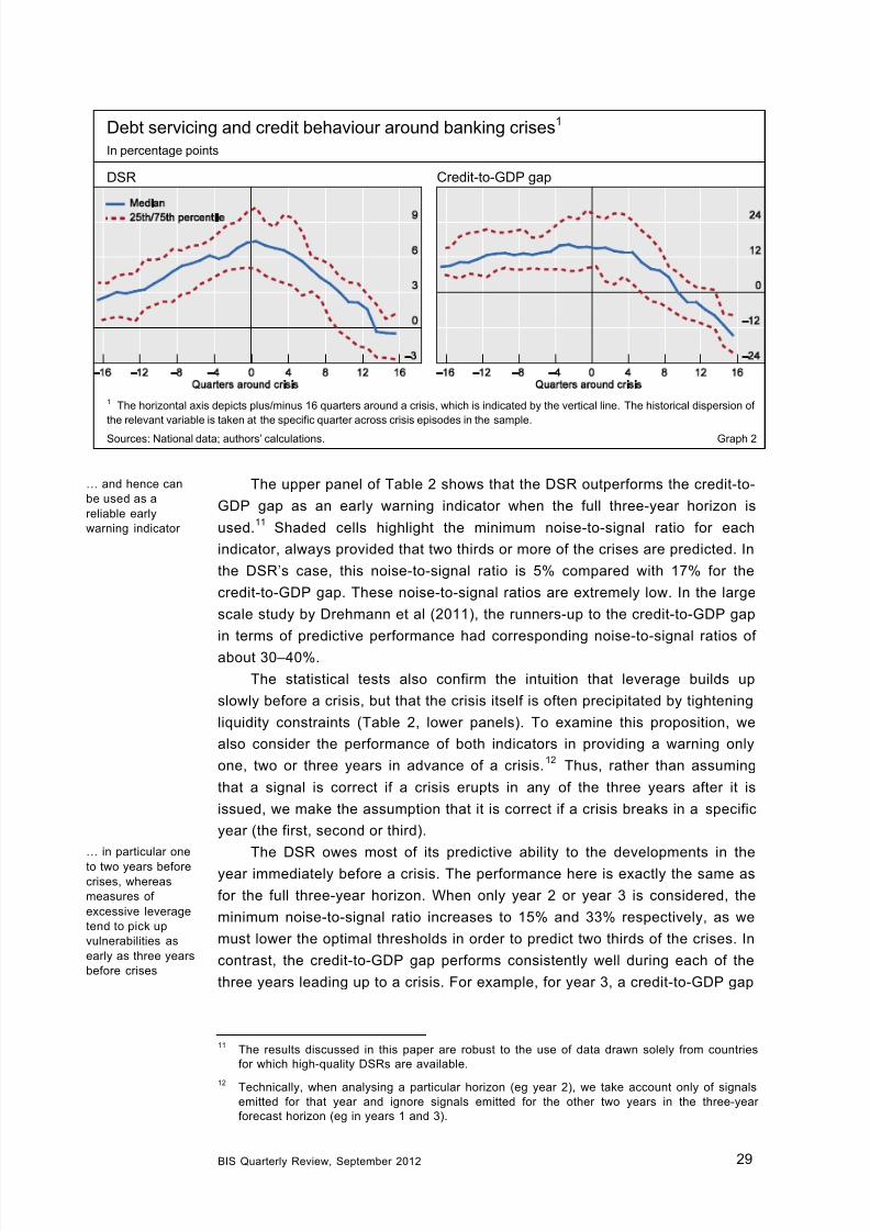
As a first step, we look at the time prof ile for both indicator variables

around systemic banking crises. Graph 2 summarises the behaviour of the

variables during a window of 16 quarters before and after the onset of a crisis(time 0 in the graphs). For each variable, we show the median (solid line) as

well as the 25th and 75th percentiles (dashed lines) of the distribution across

episodes. In both cases, a value of zero corresponds to the average conditions

outside the 33-quarter window.9

The graph shows that both the DSR and the credit-to-GDP gap are very

high in the run-up to crises, albeit with different time profiles. The median DSR

starts from a relatively low base and triples during the four years before a

crisis, at which point it peaks. The credit-to-GDP gap, on the other hand, is

already very high three to four years ahead of a crisis but rises much more

slowly. These developments can be interpreted in terms of the slow andcontinuous build-up of leverage before the crisis. Ultimately, though, crises

erupt when the incipient liquidity constraint captured by the DSR starts to bind.

For early warning purposes, Graph 2 suggests that both indicators should be

useful, but that the DSR may perform better over shorter horizons and the

credit-to-GDP gap over longer ones.

To assess the early warning performance of each indicator, we use a

signal extraction method as first proposed in this type of context by Kaminsky

and Reinhart (1999). The underlying idea is simple: a particular indicator will

give a signal if it breaches a predefined threshold. We consider a signal correct

if a crisis occurs at any point within the following three years. Otherwise, weconsider it incorrect (a false positive). The noise-to-signal ratio is the fraction of

false positives relative to the fraction of correct signals. The lower this ratio, the

better the signalling quality of the indicator. As the costs of false positives are

much lower than those of failing to predict a crisis, we search across a wide

range of thresholds to select the one that keeps the noise-to-signal ratio to a

minimum while predicting at least two thirds of the cr ises.10

8Combining the credit-to-GDP gap with indicators that capture accelerating asset price growth

such as the property price and equity price gaps can provide better early warning indicators

(Borio and Drehmann (2009)).

9

Outside the 33-quarter window, the DSR has a mean of –0.1 and the credit-to-GDP gap oneof 1.2.

10See Borio and Drehmann (2009) for a more detailed discussion of this issue.

DSRs tend to rise

sharply before

crises and decline

rapidly in their

aftermath …




Debt servicing and credit behaviour around banking crises1


DSR Credit-to-GDP gap

1 The horizontal axis depicts plus/minus 16 quarters around a crisis, which is indicated by the vertical line. The historical dispersion of

the relevant variable is taken at the specific quarter across crisis episodes in the sample.

Sources: National data; authors’ calculations. Graph 2

The upper panel of Table 2 shows that the DSR outperforms the credit-to-

GDP gap as an early warning indicator when the full three-year horizon is

used.11

Shaded cells highlight the minimum noise-to-signal ratio for each

indicator, always provided that two thirds or more of the crises are predicted. In

the DSR’s case, this noise-to-signal ratio is 5% compared with 17% for the

credit-to-GDP gap. These noise-to-signal ratios are extremely low. In the large

scale study by Drehmann et al (2011), the runners-up to the credit-to-GDP gap

in terms of predictive performance had corresponding noise-to-signal ratios of

about 30–40%.

The statistical tests also confirm the intuition that leverage builds up

slowly before a crisis, but that the crisis itself is often precipitated by tightening

liquidity constraints (Table 2, lower panels). To examine this proposition, we

also consider the performance of both indicators in providing a warning only

one, two or three years in advance of a crisis.12

Thus, rather than assuming

that a signal is correct if a crisis erupts in any of the three years after it is

issued, we make the assumption that it is correct if a crisis breaks in a specific

year (the first, second or third).

The DSR owes most of its predictive ability to the developments in the

year immediately before a crisis. The performance here is exactly the same as

for the full three-year horizon. When only year 2 or year 3 is considered, the

minimum noise-to-signal ratio increases to 15% and 33% respectively, as we

must lower the optimal thresholds in order to predict two thirds of the crises. In

contrast, the credit-to-GDP gap performs consistently well during each of the

three years leading up to a crisis. For example, for year 3, a credit-to-GDP gap

11The results discussed in this paper are robust to the use of data drawn solely from countries

for which high-quality DSRs are available.

12Technically, when analysing a particular horizon (eg year 2), we take account only of signals

emitted for that year and ignore signals emitted for the other two years in the three-year

forecast horizon (eg in years 1 and 3).

… and hence can

be used as a

reliable early

warning indicator

… in particular one

to two years before

crises, whereas

measures of

excessive leverage

tend to pick up

vulnerabilities as

early as three years

before crises




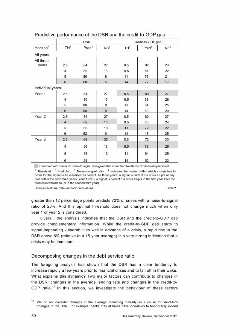
Predictive performance of the DSR and the credit-to-GDP gap

DSR Credit-to-GDP gap

Horizon4

TH1

Pred2 NS3 TH1 Pred2 NS3

All years

All three

years 2.5 84 27 8.5 92 23

4 80 13 9.5 84 22

5 80 8 11 76 21

6 68 5 14 72 17

Individual years

Year 1 2.5 84 27 8.5 80 27

4 80 13 9.5 68 28

5 80 8 11 64 25

6 68 5 14 60 20

Year 2 2.5 84 27 8.5 80 274 68 15 9.5 80 24

5 60 10 11 72 22

6 52 6 14 48 25

Year 3 2.5 68 33 8.5 72 30

4 56 18 9.5 72 26

5 48 13 11 64 25

6 28 11 14 52 23

Threshold with minimum noise-to-signal ratio given that more than two thirds of crises are predicted.

1Threshold.

2Predicted.

3Noise-to-signal ratio.

4Indicates the horizon within which a crisis has to

occur for the signal to be classified as correct. All three years: a signal is correct if a crisis erupts at anytime within the next three years. Year 1 (2/3): a signal is correct if a crisis erupts in the first year after the

prediction was made (or in the second/third year).

Sources: National data; authors’ calculations. Table 2

greater than 12 percentage points predicts 72% of crises with a noise-to-signal

ratio of 26%. And this optimal threshold does not change much when only

year 1 or year 2 is considered.

Overall, the analysis indicates that the DSR and the credit-to-GDP gap

provide complementary information. While the credit-to-GDP gap starts to

signal impending vulnerabilities well in advance of a crisis, a rapid rise in the

DSR above 6% (relative to a 15-year average) is a very strong indication that a

crisis may be imminent.

Decomposing changes in the debt service ratio

The foregoing analysis has shown that the DSR has a clear tendency to

increase rapidly a few years prior to financial crises and to fall off in their wake.

What explains this dynamic? Two major factors can contribute to changes in

the DSR: changes in the average lending rate and changes in the credit-to-

GDP ratio.13

In this section, we investigate the behaviour of these factors

13We do not consider changes in the average remaining maturity as a cause for short-term

changes in the DSR. For example, banks may at times have incentives to temporarily extend




before and after crises, and discuss their implications for the monetary

transmission channel.

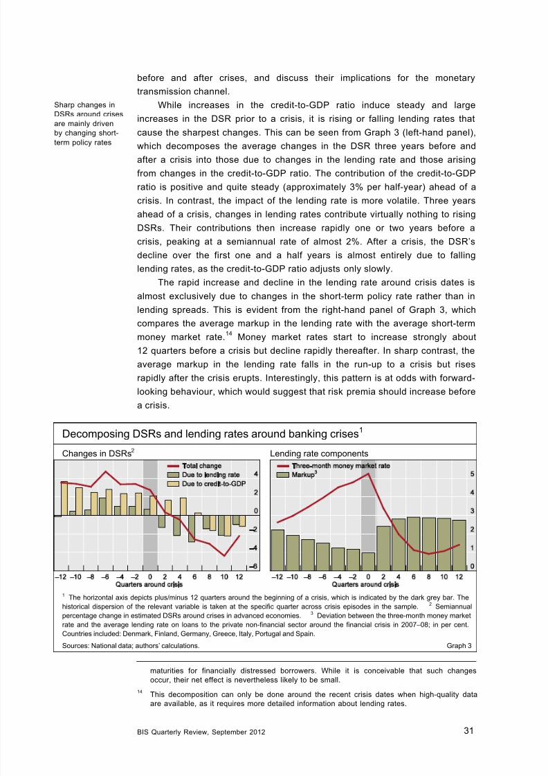
While increases in the credit-to-GDP ratio induce steady and large

increases in the DSR prior to a crisis, it is rising or falling lending rates that

cause the sharpest changes. This can be seen from Graph 3 (left-hand panel),which decomposes the average changes in the DSR three years before and

after a crisis into those due to changes in the lending rate and those arising

from changes in the credit-to-GDP ratio. The contribution of the credit-to-GDP

ratio is positive and quite steady (approximately 3% per half-year) ahead of a

crisis. In contrast, the impact of the lending rate is more volatile. Three years

ahead of a crisis, changes in lending rates contribute virtually nothing to rising

DSRs. Their contributions then increase rapidly one or two years before a

crisis, peaking at a semiannual rate of almost 2%. After a crisis, the DSR’s

decline over the first one and a half years is almost entirely due to falling

lending rates, as the credit-to-GDP ratio adjusts only slowly.The rapid increase and decline in the lending rate around crisis dates is

almost exclusively due to changes in the short-term policy rate rather than in

lending spreads. This is evident from the right-hand panel of Graph 3, which

compares the average markup in the lending rate with the average short-term

money market rate.14

Money market rates start to increase strongly about

12 quarters before a crisis but decline rapidly thereafter. In sharp contrast, the

average markup in the lending rate falls in the run-up to a crisis but rises

rapidly after the crisis erupts. Interestingly, this pattern is at odds with forward-

looking behaviour, which would suggest that risk premia should increase before

a crisis.

maturities for financially distressed borrowers. While it is conceivable that such changes

occur, their net effect is nevertheless likely to be small.14

This decomposition can only be done around the recent crisis dates when high-quality data

are available, as it requires more detailed information about lending rates.

Decomposing DSRs and lending rates around banking crises1

Changes in DSRs2

Lending rate components

1 The horizontal axis depicts plus/minus 12 quarters around the beginning of a crisis, which is indicated by the dark grey bar. The

historical dispersion of the relevant variable is taken at the specific quarter across crisis episodes in the sample.2

Semiannual

percentage change in estimated DSRs around crises in advanced economies. 3 Deviation between the three-month money market

rate and the average lending rate on loans to the private non-financial sector around the financial crisis in 2007–08; in per cent.

Countries included: Denmark, Finland, Germany, Greece, Italy, Portugal and Spain.

Sources: National data; authors’ calculations. Graph 3

Sharp changes in

DSRs around crises

are mainly driven

by changing short-term policy rates




These patterns suggest that the impact of interest rate changes on the

DSR constitute an important additional way in which monetary policy is

transmitted to the real economy. An increase (reduction) in nominal interest

rates leads to higher (lower) lending rates that raise (lower) DSRs. As we have

shown in the previous sections, high DSRs increase output volatility and canlead to a financial crisis. Of course, changing the policy stance may also

influence both credit and income via other channels.15

This will affect the DSR

to the extent that the credit-to-income ratio changes. Because an interest rate

change is only gradually transmitted to credit and income and tends to move

them in the same direction, however, it may take considerable time before

there is a notable impact on their ratio. This seems to be the case in Graph 3.

The left-hand panel shows that the change in the credit-to-GDP ratio remains

approximately constant until a crisis occurs (and a few quarters beyond) even

though money market rates are steadily increasing over the same period (right-

hand panel).

15Mishkin (1996) provides an overview of the various channels of monetary transmission. In

terms of Mishkin’s terminology, the “debt cost” channel that we discuss here seems to belong

under the more general “credit channel”.

Household and business sector DSRs


Australia Finland

Italy United States

The red vertical lines indicate the initial date of a banking crisis. The shaded areas represent recession periods as identified by the

algorithm suggested by Harding and Pagan (2002), except for the United States, where NBER recession dates are used.

Sources: NBER; authors’ calculations. Graph 4




DSRs for the household and the business sector

To assess whether increases in aggregate DSRs are driven by the debt

situation of households or businesses, this section derives separate DSRs for

each sector. The data required to do so, however, are only available for a

subset of countries.16 An additional complication arises from the question of

how to divide GDP between the two sectors. We sidestep this problem by using

disposable income for the household sector and the corporate operating

surplus for the business sector.

The sector-specific DSRs reveal that sectoral vulnerabilities may not

always build up at the same time. As examples, Graph 4 depicts these ratios

for Australia, Finland, Japan and the United States. The graph shows that the

DSRs in the two sectors can, at times, display significantly different patterns.

For instance, in the United States, the business sector DSR seems to be more

closely linked to the standard business cycle, whereas household sector DSRs

only peak ahead of a crisis. Also, the Australian business sector’s DSR did not

peak after the recent global crisis, in sharp contrast to the corresponding

household sector pattern.

16Sectoral DSRs can be constructed for Australia, Denmark, Finland, Italy, Japan, Norway,

Portugal, Spain, the United Kingdom and the United States.

Sectoral DSRs are

consistent with

existing estimates

and can reveal

differentvulnerabilities for

the household and

the business sector

Comparison of DSR estimates

Deviations from mean in percentage points

Australia Italy Norway

Portugal Spain United States

Sources: US Federal Reserve System; IMF; national data; authors’ calculations. Graph 5




The household sector DSRs confirm that our method of constructing DSRs

with relatively little information results in approximations that appear

remarkably consistent when compared with estimates by the IMF and the Fed.

In particular, the latter uses much more granular data (Dynan et al (2003)). The

average difference between our US estimates and those of the Fed and theIMF are –0.41% and 0.84% respectively. For the remaining countries, the

levels of DSR estimates provided by the IMF differ from ours. One likely

explanation is that the IMF approximates credit by different series. The cyclical

patterns, though, are exceptionally well aligned. This is clear from Graph 5,

which shows the deviations of different household sector DSR estimates from

their respective means in countries where such a comparison is possible.

Concluding remarks

In this special feature, we have discussed the DSR’s capabilities as anindicator for private sector indebtedness. We have found that its level is

associated with the loss of output in subsequent economic downturns and that

it provides a fairly accurate signal for an impending financial crisis, albeit at

shorter horizons than alternative measures.

This suggests the benefits of monitoring the debt service costs in the

economy. It also indicates that policymakers should act early when choosing to

lean against credit booms, before the DSR reaches critical levels.

Despite these promising results, several data-related issues need to be

resolved before more accurate DSR estimates can be produced. Data for the

average interest rate and remaining maturity of the outstanding credit stockwould be particularly useful. Currently, this type of data exists only for the most

recent decade and for a small set of industrialised countries. A broader

coverage would permit a deeper characterisation of the linkages between

short-run policy rates and the DSR. Such an analysis would potentially be

useful for policy.




References:

Borio, C and M Drehmann (2009): “Assessing the risk of banking crises –

revisited”, BIS Quarterly Review, March, pp 29–46.

Borio, C and P Lowe (2002): “Assessing the risk of banking crises”, BIS

Quarterly Review, December, pp 43–54.

Cecchetti, S, M Kohler and C Upper (2009): “Financial crises and economic

activity”, NBER Working Papers, no 15379.

Drehmann, M, C Borio and K Tsatsaronis (2011): “Anchoring countercyclical

capital buffers: the role of credit aggregates”, International Journal of Central

Banking, no 7.

Dynan, K, K Johnson and K Pence (2003): “Recent changes to a measure of

US household debt service”, Federal Reserve Bulletin, vol 89, pp 417–26.

Harding, D and A Pagan (2002): “Dissecting the cycle: a methodological

investigation”, Journal of Monetary Economics, vol 49, pp 365–81.

Juselius, M and M Kim (2011): “Sustainable financial obligations and crisis

cycles”, Helsinki Center of Economic Research Discussion Papers, no 313.

Kaminsky, G and C Reinhart (1999): “The twin crises: the causes of banking

and balance-of-payments problems”, Amer ican Economic Review , no 89,

pp 473–500.

Laeven, L and F Valencia (2012): “Systemic banking crises database: an

update”, IMF Working Papers, no WP/12/163.

Mishkin, F (1996): “The channels of monetary transmission: lessons for

monetary policy”, NBER Working Papers, no 5464.

Reinhart, C and K Rogoff (2008): “Banking crises: an equal opportunity

menace”, NBER Working Papers, no 14587.

debt service and private sector

Documents