1

Decentralized Civil Structural Control using Real-time Wireless Sensing and Embedded Computing

Yang Wang a, R. Andrew Swartz b, Jerome P. Lynch *b, Kincho H. Law a,

Kung-Chun Lu c, Chin-Hsiung Loh c

a Dept. of Civil and Environmental Engineering, Stanford Univ., Stanford, CA 94305, USA b Dept. of Civil and Environmental Engineering, Univ. of Michigan, Ann Arbor, MI 48109, USA

c Dept. of Civil Engineering, National Taiwan Univ., Taipei, Taiwan * Correspondence Author: Jerome P. Lynch Assistant Professor Department of Civil and Environmental Engineering The University of Michigan 2380 G. G. Brown Building Ann Arbor, MI 48109-2125 USA Email: jerlynch@umich.edu

Abstract Structural control technologies have attracted great interest from the earthquake engineering

community over the last few decades as an effective method of reducing undesired structural

responses. Traditional structural control systems employ large quantities of cables to connect

structural sensors, actuators, and controllers into one integrated system. To reduce the high-costs

associated with labor-intensive installations, wireless communication can serve as an alternative

real-time communication link between the nodes of a control system. A prototype wireless

structural sensing and control system has been physically implemented and its performance

verified in large-scale shake table tests. This paper introduces the design of this prototype system

and investigates the feasibility of employing decentralized and partially decentralized control

strategies to mitigate the challenge of communication latencies associated with wireless sensor

networks. Closed-loop feedback control algorithms are embedded within the wireless sensor

prototypes allowing them to serve as controllers in the control system. To validate the

embedment of control algorithms, a 3-story half-scale steel structure is employed with

magnetorheological (MR) dampers installed on each floor. Both numerical simulation and

experimental results show that decentralized control solutions can be very effective in attaining

the optimal performance of the wireless control system.

Key words: structural control, wireless communication, embedded computing, decentralized control, velocity feedback control

2

1. Introduction

As an effective method of reducing the dynamic response of structures during earthquakes or

typhoons, structural control technologies have attracted a great amount of interest from structural

engineering researchers and practitioners over the past few decades (Soong and Spencer, 2002).

About 50 buildings and towers were instrumented with various types of structural control systems

from 1989 to 2003 (Chu et al., 2005), with evident reduction in structural dynamic responses

being reported. Current structural control systems can be categorized into three major types: (a)

passive control (e.g. base isolation), (b) active control (e.g. active mass dampers), and (c) semi-

active control (e.g. semi-active variable dampers). Passive control has the advantage of power

efficiency, while active control has the advantage of being adaptable to real-time excitations. As

a hybrid between these two approaches to structural control (active and passive), semi-active

control effectively combines the advantages of both systems. Examples of semi-active actuators

include active variable stiffness (AVS) devices, semi-active hydraulic dampers (SHD),

electrorheological (ER) dampers, and magnetorheological (MR) dampers. Another attractive

feature of semi-active control systems is that they are inherently stable because their actuators do

not apply mechanical energy directly to the structure.

In both semi-active and active control systems, sensors are employed in the structure to collect

real-time structural response data during dynamic excitation (e.g. wind or earthquake). The

response data is then fed into a single or multiple control decision modules (controllers) in order

to determine control forces and apply commands to system actuators in real-time. According to

these command signals, the structural actuators generate control forces intended to reduce

unwanted structural vibrations. In traditional semi-active or active control systems, coaxial wires

are normally used to provide communication links between sensors, actuators and controllers.

For a typical low-rise building, the installation of a commercial wire-based data acquisition (DAQ)

system can cost upwards of a few thousand dollars per sensing channel (Celebi, 2002). As the

3

size of the control system grows (defined by the nodal density and inter-nodal spatial distances),

the additional cabling needed may result in increases in installation time and expense (Solomon et

al., 2000). To capitalize on future low-cost semi-active devices that are densely installed in a

structure, wireless communication technology can be adopted to eradicate the coaxial cables

associated with traditional control systems. Although wireless communication has been widely

explored for use in structural monitoring applications (Straser and Kiremidjian, 1998; Lynch and

Loh, 2006a; Wang et al., 2007), application to real-time feedback control in structural

engineering has been scarce (Lynch and Tilbury, 2005). Outside of structural engineering, a few

examples of wireless control systems have been reported (Eker et al., 2001; Ploplys et al., 2004).

When replacing wired communication channels with wireless ones for feedback structural control,

difficulties include coordination of the wireless nodes in a collaborative control network,

degradation of real-time performance, and higher probability of data loss during transmission.

The degradation of the control system’s real-time characteristics is a common problem faced by

distributed network control systems, regardless of using wired or wireless communication (Lian

et al., 2002). Among the different solutions proposed for this problem, one possible remedy is

the adoption of decentralized control strategies (Sandell et al., 1978; Lynch and Law, 2002). In a

decentralized control system, the sensing and control network is divided into multiple subsystems.

Controllers are assigned to each subsystem and require only subsystem sensor data to make

control decisions. Therefore, reduced use of the communication channel is offered by a

decentralized control architecture, which results in higher control sampling rates. Furthermore,

decentralized control requires relatively shorter communication ranges, enabling more reliable

wireless data transmissions. The drawback of decentralized control is that decentralized system

architectures may only achieve sub-optimal control performance compared with centralized

counterparts, because each subsystem only has its own state data from which it must calculate

4

control decisions. This work attempts to investigate the effectiveness of decentralized wireless

control in civil structures.

This paper first introduces a prototype wireless structural sensing and control system developed

by the authors (Wang et al., 2006). The system consists of multiple stand-alone wireless sensors

that form an integrated network through a common wireless communication channel. Each

wireless sensor can record response data from sensors, calculate control forces, communicate

state data, and command actuators. In order to investigate the effects of communication latencies

on centralized and decentralized wireless control strategies, centralized and decentralized output

feedback control algorithms are implemented. The decentralized control method is developed by

applying appropriate shape constraints to the gain matrix of a normal optimal output feedback

control problem. Numerical simulations show that the higher sampling rates achievable by

decentralized control may compensate for the disadvantage of incomplete sensor data from which

control decisions are made. Large-scale shake table experiments are conducted on a 3-story steel

frame structure installed with MR dampers to compare the performance of different decentralized

and centralized control schemes.

2. A Prototype Real-time Wireless Sensing and Control System

To illustrate the architecture of the prototype wireless sensing and control system, Fig. 1 shows a

3-story structure controlled by three actuators. Wireless sensors and controllers are mounted on

the structure for measuring structural response data and commanding actuators in real-time.

Besides the wireless sensing and control units that are necessary for data collection and the

operation of the actuators, a remote command server with a wireless transceiver is included in the

system to initiate the operation of the control system and to log the flow of wireless data. To

initiate the operation of the control system, the command server first broadcasts a start signal to

all of the wireless sensing and control units. Once the start command is received, the wireless

5

units that are responsible for collecting sensor data start acquiring and broadcasting data at a

preset time interval. Accordingly, the wireless units responsible for commanding the actuators

receive the sensor data, calculate desired control forces, and apply control commands within the

specified time interval allotted at each time step. The following describes in detail the design of

the wireless sensing and control units. Specific attention is paid to the control signal generation

and wireless communication modules of the wireless unit since both are integral to the

performance of the global control system.

2.1 Hardware Design for the Wireless Sensing and Control Unit

The wireless unit is designed in such a way that the unit can serve as either a sensing unit (i.e. a

unit that collects data from sensors and wirelessly transmits the data), a control unit (i.e. a unit

that calculates control forces and commands actuators), or a unit for both sensing and control.

This flexibility is supported by an integrated hardware design based upon a wireless sensing unit

previously proposed for wireless structural monitoring by Wang et al. (2007). Three basic

functional modules are included in the wireless sensing unit design: sensor signal digitizer,

computational core, and wireless transceiver. The wireless control unit contains the same three

modules as the wireless sensing unit, but also includes a supplementary control signal generation

module designed to reside off-board of the basic wireless sensor. The architectural design of the

wireless control unit is presented in Fig. 2(a). The architectural design of the wireless sensing

unit can be obtained by simply omitting the control signal generation module. A simple two-

layer printed circuit board (PCB) for the wireless sensing unit is designed and fabricated (Fig. 2b).

As shown in Fig. 2(c), the PCB, wireless transceiver, and batteries are stored within an off-the-

shelf weatherproof plastic container, which has the dimensions of 10.2cm by 6.5cm by 4.0cm.

The sensor signal digitization module of the wireless unit contains a 4-channel 16-bit Texas

Instrument ADS8341 analog-to-digital (A/D) converter. This module converts the 0 to 5V analog

6

output of up to four sensors (to date, different types of transducers have been successfully

interfaced including accelerometers, velocity meters, LVDTs and strain gages) into digital

formats usable by the wireless sensor’s computational core. The digitized sensor data is

transferred to the computational core through a high-speed serial peripheral interface (SPI) port.

The computational core consists of a low-power 8-bit Atmel ATmega128 microcontroller and an

external 128kB static random access memory (SRAM) chip for data storage. For wireless

communication among the sensing units, two types of wireless transceivers may be employed:

900MHz MaxStream 9XCite and 2.4GHz MaxStream 24XStream (MaxStream, 2005). Generally,

the 9XCite is used in the U.S. and other countries where 900MHz is open to unlicensed usage

while the 24XStream is used internationally on the 2.4GHz radio band. When a wireless unit is

designated as a sensing unit, its wireless transceiver is primarily used to send sensor data out to

the wireless network. In contrast, for a wireless control unit, its wireless transceiver receives

sensor data from the network. After receiving the sensor data, the ATmega128 microcontroller

embedded in the wireless control unit computes the desired control forces. Once the control force

calculation is completed, the wireless control unit issues commands (voltage signals) to the

actuator through the control signal generation module. All of the hardware components of the

wireless sensing unit, not including the wireless transceiver, consume about 32mA when active

and 80µA when in stand-by mode. The additional power consumption of the two wireless

transceivers (9XCite and 24XStream) will be presented in section 2.3.

2.2 Control Signal Generation Module

A separate hardware module is designed to be connected with the wireless sensing unit, which

permits the unit to generate analog voltage signals for commanding actuators. At the core of this

control signal generation module is the single-channel 16-bit digital-to-analog (D/A) converter,

the Analog Device AD5542. The AD5542 receives a 16-bit unsigned integer from the

ATmega128 and converts the integer value to an analog voltage output spanning from -5 to 5V.

7

Additional support electronics are included in the control signal generation module to offer stable

zero-order hold voltage outputs at high sampling rates (1 MHz maximum). The wide voltage

output range (-5 to 5V) of the control signal generation module, particularly the negative output

range, is one of the key features of the module’s design. With the wireless sensing unit designed

to operate on 5V, the Texas Instruments PT5022 switching regulator is integrated in the signal

generation module to convert the 5V regulated power supply into a stable -5V reference. Another

auxiliary component required for the AD5542 to generate a bipolar -5 to 5V output signal is a

rail-to-rail input and output operational amplifier, for which the National Semiconductor

LMC6484 operational amplifier is selected. The typical slew rate of the LMC6484 is about

1.3V/µs, which means that the output voltage can swing about 1.3V within 1µs. This output

gradient is compatible with the microsecond-level settling time of the AD5542 D/A converter.

When operational, the control signal generation module draws about 70mA from the 5V power

supply provided by the wireless sensing unit.

As shown in Fig. 3(a), a separate double-layer printed circuit board (PCB) is designed to

accommodate the D/A converter (AD5542) and its auxiliary electrical components. The control

signal board is attached via two multi-line wires to the wireless sensor. To reduce circuit noise,

two separate wires are used with one dedicated to analog signals and the other to digital signals.

The analog signal cable transfers an accurate +5V reference voltage from the existing wireless

sensing board to the signal generation module. The digital signal cable provides all of the

connections required to accommodate the serial peripheral interface (SPI) between the

ATmega128 microcontroller and the AD5542. To command an actuator, a third wire is needed to

connect the output of the control signal generation module with the structural actuator. The

control signal generation module connected to the wireless sensing unit is shown in Fig. 3(b).

2.3 Wireless Communication Module

8

A challenge associated with employing wireless sensors in a structural control system is the

performance of the wireless communication channel. When the wireless sensors are used within

a wireless structural monitoring system, robust send-acknowledgement communication protocols

are used to ensure that no data is lost (Lynch et al., 2006b). However, the real-time requirements

of the control system do not permit sufficient time for the use of send-acknowledgement

communication protocols that ensure channel reliability. Furthermore, stochastic delays in the

channel are probable; these delays cannot be deterministically accounted for a priori in the

control solution formulation (Seth et al., 2004). For these reasons, an appropriate wireless

transceiver that minimizes data loss without sacrificing communication speed must be judiciously

selected for use in the wireless control system.

The wireless sensing unit is designed to be operable with two different wireless transceivers:

900MHz MaxStream 9XCite and 2.4GHz MaxStream 24XStream. Pin-to-pin compatibility

between these two wireless transceivers makes it possible for them to share the same hardware

connections in the wireless unit. Because of the different data rates, embedded software for using

the two transceivers is slightly different. This dual-transceiver support offers the wireless sensing

and control unit more flexibility in terms of not only use in different geographical areas, but also

provides different data transfer rates, communication ranges, and power consumption

characteristics. Table 1 summarizes the key performance parameters of the two wireless

transceivers. As shown in the table, the data transfer rate of the 9XCite is twice that of the

24XStream, while the 24XStream provides a longer communication range but consumes more

battery power. The peer-to-peer communication capability of the two wireless transceivers

makes it possible for the wireless sensing and control units to communicate with each other, thus

supporting flexible information flow among multiple wireless units. In this study, validation tests

of the wireless sensing and control system are performed using a test structure at the National

Center for Research on Earthquake Engineering (NCREE) in Taipei, Taiwan. Because of the

9

local frequency band requirements in Taiwan, the MaxStream 24XStream wireless transceiver

operating on the 2.4GHz spectrum is employed for the experimental tests.

As previously discussed, one critical issue in applying wireless communication technology to

real-time feedback structural control problems is the communication latency encountered when

transmitting sensor data from the wireless sensing units to the wireless control units. The

anticipated transmission time of the 24XStream radio for a single data packet is illustrated in Fig.

4. The transmission time consists of the communication latency (TLatency) of the radios and the

time to transfer data between the microcontroller and the radio using the universal asynchronous

receiver and transmitter (UART) interface (TUART). Assume that the data packet to be transmitted

contains N bytes and the UART data rate is RUART bps (bits per second), which is equivalent to

RUART /10 bytes per second, or RUART /10000 bytes per millisecond. It should be noted that the

UART transmits 10 bits for every one byte (8-bits) of sensor data due to start and stop bits. The

communication latency in a single transmission of this data packet can be estimated as:

10000SingleTransm Latency

UART

NT TR

= + (ms) (1)

In the prototype wireless sensing and control system, the setup parameters of the 24XStream

transceiver are first tuned to minimize the transmission latency, TLatency. Then experiments are

conducted to measure the actual TLatency, which turns out to be 15±0.5ms. The UART data rate of

the 24XStream radio, RUART, can be selected among seven different options, ranging from 1200

bps to 57600 bps. After considering the UART performance of the ATmega128 microcontroller

operated at 8MHz, RUART is selected as 38400 bps in the implementation. If a data packet sent

from a sensing unit to a control unit contains 11 bytes, the total time delay for a single

transmission is estimated to be:

10

10000 1115 17.8638400SingleTransmT ×= + ≈ (ms) (2)

This single-transmission delay represents the communication constraint that needs to be

considered when calculating the upper bound for the maximum sampling rate for the control

system. Another deciding factor for the sampling rate is the number of wireless transmissions

needed at each control sampling step. A few milliseconds of safety cushion time at each

sampling step is a prudent addition that allows a certain amount of randomness in the wireless

transmission latency without undermining the reliability of the communication system. It should

be noted that the transmission latency, TLatency, for a MaxStream 9XCite transceiver can be as low

as 5ms. This lower latency makes the 9XCite transceiver more suitable for real-time feedback

control applications compared with the 24XStream transceiver. However, the 9XCite transceiver

may only be used in countries where the 900MHz band is for free public usage, such as the U.S.,

Canada, Mexico, South Korea, and Japan.

3. Centralized and Decentralized Time-delay Control Algorithms using Velocity Feedback

An optimal feedback control design normally requires adequate real-time structural response data

to compute optimal control forces. For example, if a multi-story building is modeled by a

lumped-mass structural system with actuators deployed among adjacent floors, real-time floor

displacements and velocities that constitute the state-space vector are needed for a typical linear

quadratic regulator (LQR) controller (Franklin et al., 2003). However, due to instrumentation

complexity and cost, not all structural response data may be available in practice. To address this

difficulty, output feedback control methods can be used to provide an optimal control strategy

under the constraint that only part of the state-space variables are measured in real-time. This

section first presents the basic formulation of an optimal centralized output feedback control

11

solution and then proposes a modified algorithm that allows the output feedback gain matrix to be

constrained. The output feedback gain matrix is then formulated for various decentralized control

architectures using the constrained gain matrix algorithm detailed herein.

3.1 Formulation for Centralized Linear Output Feedback Control

The output feedback digital-domain LQR control solution can be briefly summarized as follows.

For a lumped-mass structural model with n degrees-of-freedom (DOF) and m actuators, the

system state-space equation considering l time steps of delay can be stated as:

[ ] [ ] [ ]1k k k l+ = + −d d d d dz A z B p , where [ ] [ ][ ]k

kk

⎧ ⎫⎪ ⎪= ⎨ ⎬⎪ ⎪⎩ ⎭

dd

d

xz

x (3)

Here, [ ]kdz represents the 2n × 1 discrete-time state-space vector, [ ]kdx is the relative (to the

base) displacement of the structural degrees-of-freedom, [ ]k l−dp is the delayed m × 1 control

force vector, dA is the 2n × 2n system matrix (containing the information about structural mass,

stiffness and damping), and dB is the 2n × m actuator location matrix. The primary objective of

the time-delay LQR problem is to minimize a global cost function, J, by selecting an optimal

control force trajectory dp :

[ ] [ ] [ ] [ ]( ) 2 2, where 0 and 0T Tn n m m

k lJ k k k l k l

∞

× ×=

= + − − ≥ >∑dp d d d dz Qz p Rp Q R (4)

In an output feedback control design, when control decisions are computed, only data in the

system output vector [ ]kdy are available. The output vector is defined by a q × 2n linear

transformation, dD , to the state-space vector [ ]kdz :

12

[ ] [ ]k k=d d dy D z (5)

For example, if the relative velocities on all floors are measurable but no relative displacement is

measurable, dD can be defined as:

[ ]n n n n× ×=d_cenD 0 I (6)

In another example, if only inter-story velocities between adjacent floors are measurable, the

following output matrix dD can be used:

0 0 0 1 0 00 0 0 1 1 0 0 0 0 0 1 1

⎡ ⎤⎢ ⎥= −⎢ ⎥⎢ ⎥−⎣ ⎦

d_decD (7)

The m × q optimal gain matrix dG is required to provide a linear output feedback control:

[ ] [ ]k k=d d dp G y (8)

Chung et al. (1995) proposes a solution to the output feedback control problem with time delay

(say, l time steps) by introducing a modified first-order difference equation:

[ ] [ ] [ ]1k k k+ = +d d d d dz A z B p (9)

in which the augmented state [ ]kdz is assembled from the past l states as:

13

[ ]

[ ][ ]

[ ] ( )2 1 1

1

n l

kk

k

k l+ ×

⎡ ⎤⎢ ⎥−⎢ ⎥= ⎢ ⎥⎢ ⎥

−⎢ ⎥⎣ ⎦

d

dd

d

zz

z

z

(10)

This system is equivalent to the original system (Eq. 3) by proper definitions of the augmented

matrices and vectors: dA and dB are the augmented state-space system matrices, dD is the

augmented output matrix, Q is the augmented weighting matrix, and ldZ is the second statistical

moment of the augmented initial disturbance. As a result, the following nonlinearly coupled

matrix equations are simultaneously solved for an optimal output feedback gain matrix dG , the

Lagrangian matrix, L, and a constant matrix, H:

( ) ( ) ( )T T T+ + − + + =d d d d d d d d d d d dA B G D H A B G D H Q D G RG D 0 (11a)

( ) ( )T

l+ + − + =d d d d d d d d dA B G D L A B G D L Z 0 (11b)

( )2 2T T T+ + =d d d d d d d d dB H A B G D LD RG D LD 0 (11c)

Interested readers are referred to Chung et al. (1995), where the time-delay optimal control

solution is derived in detail.

3.2 Heuristic Solution for Centralized and Decentralized Output Feedback Gain Matrices

An iterative algorithm to solve the continuous-time feedback control problem has been presented

by Lunze (1990). The algorithm (Fig. 5) starts from an initial estimate for the gain matrix dG .

Within each iteration step i, the matrix Hi and Li are solved respectively using the current

estimate of the gain matrix idG . Based on the Hi and Li matrices computed, a searching gradient

14

i∆ is calculated and the new gain matrix 1i+dG is computed by traversing along a gradient from

idG . An adaptive multiplier, s, is used to dynamically control the search step size. At each

iteration step, two conditions are used to decide whether 1i+dG is an acceptable estimate. The first

condition is trace( 1i l+ dH Z ) < trace( i ldH Z ) which guarantees that 1i+dG is a better solution than

idG . The second condition is that the maximum magnitude of all the eigenvalues of the matrix

( )1i++d d d dA B G D is less than 1 which ensures the stability of the augmented system.

The iterative algorithm put forth by Lunze (1990) has an inherently powerful and attractive

feature; the algorithm can be used to formulate an optimal control solution for a decentralized

system simply by constraining the structure of dG to be consistent with the decentralized

architecture. The following equation presents the structure of two decentralized output feedback

gain matrices for a simple 3-story lumped-mass structure.

1 2

* 0 0 * * 00 * 0 , and 0 * *0 0 * 0 * *

⎡ ⎤ ⎡ ⎤⎢ ⎥ ⎢ ⎥= =⎢ ⎥ ⎢ ⎥⎢ ⎥ ⎢ ⎥⎣ ⎦ ⎣ ⎦

d_dec d_decG G (12)

The pattern in 1d_decG specifies that when computing control decisions, the actuator on each floor

only needs the entry in the output vector dy that corresponds to that floor. The pattern in 2d_decG

specifies that information from neighboring floors be considered in calculating control actions. In

order to find a decentralized gain matrix that satisfies desired architectural constraints, the

algorithm described in Fig. 5 is modified by zeroing out the entries in the gradient matrix i∆

corresponding to zero terms in the decentralized output feedback gain matrix. The next estimate

1i+dG is computed by traversing along this constrained gradient. Using the above decentralized

15

gain matrices and the output matrix d_decD defined in Eq. (7), inter-story velocities between

adjacent floors can be used for the calculation of control actions in a decentralized control system.

3.3 Simulation Results using Centralized and Decentralized Control Strategies

Numerical simulations have been conducted to assess the performance of decentralized and

centralized control strategies considering time delays due to communication latencies. A

numerical model for the 3-story half-scale laboratory structure illustrated in Fig. 1 is used for the

simulation. For simplicity, ideal structural actuators which are capable of producing any desired

force under the maximum limit of 20kN is deployed between each pair of adjacent floors using

the V-braces shown. Three control architectures are employed: (1) decentralized, (2) partially

decentralized, and (3) centralized. Different patterns of the gain matrices, dG , and the output

matrices, dD , for these three control architectures are summarized in Table 2. As defined by

these matrices, one centralized and two decentralized velocity feedback patterns are adopted. An

LQR weighting matrix Q minimizing inter-story drifts over time and a diagonal weighting matrix

R are used when designing the optimal gain matrices for all the simulations presented herein.

Various combinations of centralization degrees (1: fully decentralized; 2: partially decentralized;

3: centralized) and sampling time steps ranging from 0.005s to 0.1s (at a resolution of 0.005s) are

simulated.

To assess the performance of each control scheme, three ground motion records are used for the

simulation: 1940 El Centro NS (Imperial Valley Irrigation District Station), 1999 Chi-Chi NS

(TCU-076 Station), and 1995 Kobe NS (JMA Station) earthquake records. Performance indices

proposed by Spencer et al. (1998) are adopted. In particular, two representative performance

indices employed are:

16

( )( )

,1 El Centro

Kobe,Chichi

maxmax ˆmax

it i

it i

d tPI

d t

⎧ ⎫⎪ ⎪= ⎨ ⎬⎪ ⎪⎩ ⎭

, and 2 El CentroKobe

Chichi

max ˆLQR

LQR

JPI

J

⎧ ⎫⎪ ⎪= ⎨ ⎬⎪ ⎪⎩ ⎭

(13)

where 1PI and 2PI are the performance indices corresponding to inter-story drifts and LQR cost

indices, respectively. In Eq. (13), ( )id t represents the inter-story drift between floor i (i = 1, 2, 3)

and its lower floor at time t, and ( ),

max it id t is the maximum inter-story drift over the entire time

history and among all three floors. The maximum inter-story drift is normalized by its

counterpart ( ),

ˆmax it id t , the maximum response of the uncontrolled structure. The largest

normalized ratio among the simulations for the three different earthquake records is defined as the

performance index 1PI . Similarly, the performance index 2PI is defined for the LQR control

index LQRJ , as given in Eq. (4). When computing the LQR index over time, a uniform time step

of 0.005s is used to collect the structural response data points, regardless of the sampling time

step of the control scheme; this allows one control strategy to be compared to another without

concern for the different sampling time steps used in the control solution.

Values of the two control performance indices are plotted in Fig. 6 for different combinations of

centralization degrees and sampling time steps. The plots shown in Fig. 6(a) and 6(b) illustrate

that centralization degree and sampling step have significant impact on the performance of the

control system. Generally speaking, control performance is better for higher degrees of

centralization and shorter sampling times. To better review the simulation results, the

performance indices for the three different control schemes are re-plotted as a function of

sampling time in Fig. 6(c) and 6(d). As shown in Fig. 6(c), if a partially decentralized control

system can achieve 0.04s sampling step and a centralized system can only achieve 0.08s due to

additional communication latency, the partially decentralized system can result in lower

17

maximum inter-story drifts. Similar trends are observed in Fig. 6(d), although for a given

sampling time step, the performance index 2PI for the centralized case is always lower than the

indices for the two decentralized cases.

4. Validation Experiments using a 3-story Structure Instrumented with MR Dampers

To study the potential use of the wireless sensing and control system for decentralized structural

control, validation tests are conducted at the National Center for Research on Earthquake

Engineering (NCREE) in Taipei, Taiwan. The same test structure has been used in a previous

wireless control study in which one MR damper is installed for closed-loop control (Lynch et al.

2006c). Both a baseline wired control system and a wireless sensing and control system are

employed to implement the real-time feedback control of a 3-story steel frame instrumented with

three MR dampers.

4.1 Validation Test Setup

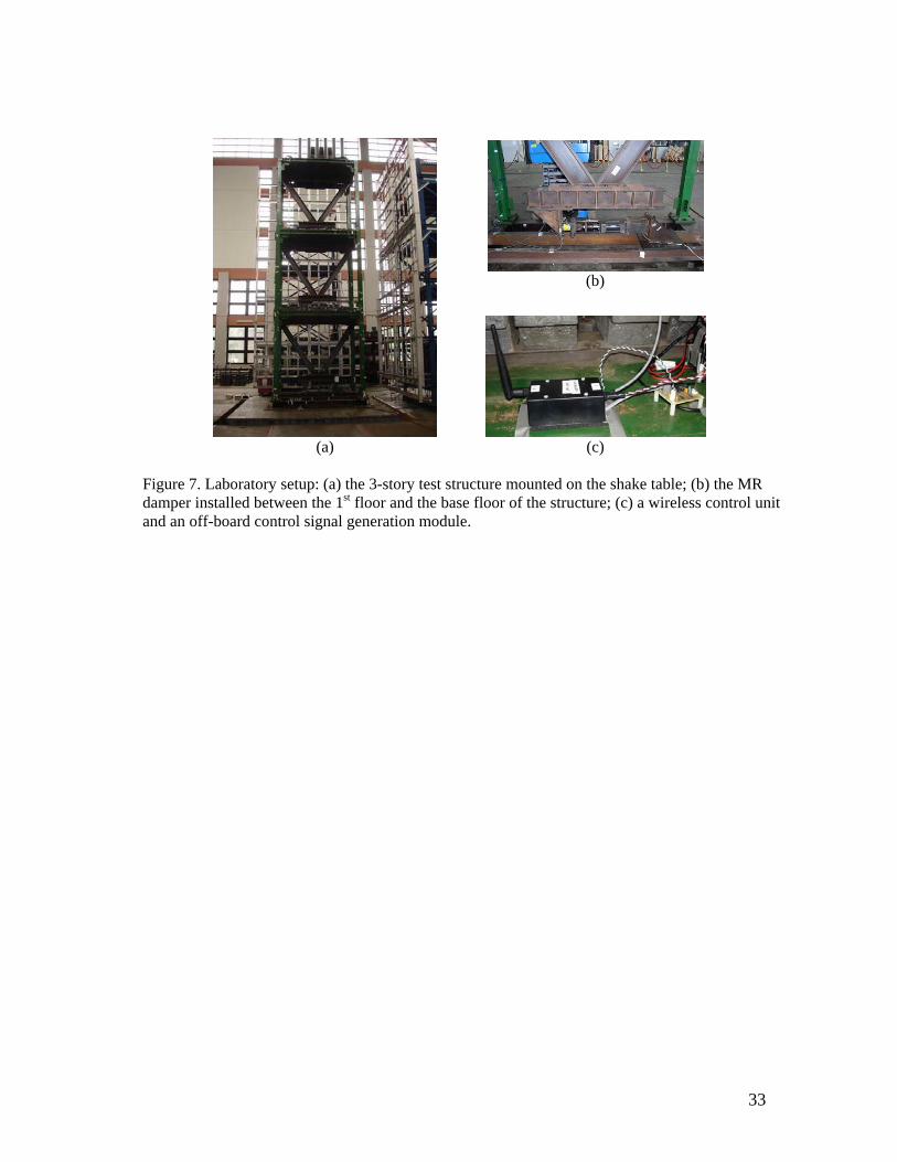
A three-story steel frame structure is designed and constructed by researchers affiliated with

NCREE (Fig. 7a). The dimensions of the structure are provided in Fig. 1. The three-story

structure is mounted on a 5m × 5m 6-DOF shake table. The shake table can generate ground

excitations with frequencies spanning from 0.1Hz to 50Hz. For this study, only longitudinal

excitations are used. Along this direction, the shake table can excite the structure with a

maximum acceleration of 9.8m/s2. The excitation has a maximum stroke and force of ±0.25m

and 220kN, respectively. The test structure and shake table are heavily instrumented with

accelerometers, velocity meters, and linear variable displacement transducers (LVDT) to measure

their dynamic response. These sensors are interfaced to a high-precision wire-based data

acquisition (DAQ) system permanently installed in the NCREE facility; the DAQ system is set to

a sampling rate of 200 Hz. A separate set of wireless sensors are installed as part of the wireless

control system.

18

For the wireless system, a total of four wireless sensors are installed following the deployment

strategy shown in Fig. 1. Each wireless sensor is interfaced to a Tokyo Sokushin VSE15-D

velocity meter to measure the absolute velocity response of each floor of the structure as well as

at the base (i.e. table top velocity). The sensitivity of the velocity meter is 10V/(m/s) with a

measurement limit of ±1 m/s. The three wireless sensors on the first three levels of the structure

(C0, C1, and C2) are also responsible for commanding the MR dampers. Besides the wireless

control system, a traditional wire-based control system is installed in the structure for

comparative analyses. Centralized and decentralized velocity feedback control schemes

described earlier (Table 2) are used for both the wired and the wireless control systems. As

shown in Table 3, different decentralization patterns and sampling steps are tested. For the test

structure, the wire-based system can achieve a sampling rate of 200Hz, or a time step of 0.005s.

Mostly decided by the communication latency of the 24XStream wireless transceivers, the

wireless system can achieve a sampling rate of 12.5Hz (or a time step of 0.08s) for the centralized

control scheme. This sampling rate is due to each wireless sensor waiting in turn to broadcast its

data to the network (about 0.02s for each transmission). An advantage of the decentralized

architecture is that fewer communication steps are needed, thereby reducing the time for wireless

communication. As shown in Table 3, the wireless system can achieve a sampling rate of

16.67Hz for partially decentralized control and 50Hz for fully decentralized control.

4.2 Magnetorheological (MR) Damper Hysteresis Model

For this experimental study, three 20 kN MR dampers are installed with V-braces on each story

of the steel structure (Fig. 7b). The damping coefficients of the MR dampers can be changed in

real-time by the wireless control units (Fig. 7(c)) simply by issuing a command voltage between 0

to 1.2V. A separate power module is needed to provide 24V of power to each MR damper. In

addition, this power module takes the command voltage as an input and converts this command

19

signal to a regulated current from 0 to 2A. The current is input to the internal electromagnetic

coil of the MR damper to generate a magnetic field that sets the viscous damping properties of the

MR fluid contained within the damper cylinder. Therefore, the axial force required to move the

damper piston against the cylinder is adjustable through the command voltage. Calibration tests

are first conducted on the MR dampers before mounting them to the structure so that modified

Bouc-Wen damper models can be formulated for each damper (Lin et al., 2005).

The nonlinear force-velocity relationship for this modified Bouc-Wen model is defined as:

( ) ( ) ( ) ( )F t C V x t z t= + (14)

where F(t) is the force provided by the MR damper, C(V) is the damping coefficient adjustable

through the damper command voltage V, ( )x t is the relative velocity of the damper piston against

the cylinder, and z(t) is the hysteresis restoring force of the damper. The hysteresis restoring

force, z(t), evolves according to the following differential equation (Lin et al., 2005):

( ) ( ) ( ) ( ) ( ) ( ) ( )1

1

N n nn

n

z t Ax t a x t z t z t x t z tβ γ−

=

⎡ ⎤= + +⎣ ⎦∑ (15)

where A, β , γ , an, and N are parametric constants of the Bouc-Wen model. The higher the order

N, the more accurate the model is in describing the complicated hysteresis behavior of the semi-

active damper. In this study, it was found that an order of N = 2 provides fairly accurate

modeling to the damper hysteresis forces. The hysteresis restoring force in discrete-time form at

step k is then rewritten as:

20

[ ] [ ] [ ] ( )1 1Tz k z k k V= − + −Φ Θ (16a)

( ) ( ) ( ) ( ) ( ) ( ){ }1 2 3 4 5T

V V V V V Vθ θ θ θ θ=Θ (16b)

[ ] [ ] [ ] [ ] [ ] [ ] [ ] [ ] [ ] [ ] [ ]{ }2 T

k t x k x k z k x k z k x k z k z k x k z k= ∆Φ (16c)

The five parameters in vector ( )VΘ are modeled as low-order polynomial functions of the

damper voltage V. Similarly, the damping coefficient, C(V), is modeled as a linear function of the

damper voltage V. For each MR damper, the constant coefficients in the polynomial functions

( )VΘ and C(V) are pre-determined and validated through a series of calibration experiments with

the damper (Lin et al., 2005). In these experiments, a displacement-controlled actuator is

employed to command displacements to the damper piston while the damper cylinder is fixed to a

reaction frame. A load cell is then used to measure the damper force, so that the force-

displacement time histories of the damper can be recorded. In order to compute the constant

coefficients in the modified Bouc-Wen model, sinusoidal and random displacement are first

applied to the damper with the damper command voltage fixed at multiple levels. Then the

model is validated through experiments when random displacement time histories are applied to

the damper with the command voltage randomly varied.

In the real-time feedback control tests, hysteresis status updating for the MR dampers is an

integral element in the calculation of damper actuation voltages. At each sampling time step, a

wireless control unit first decides the desired control force for the MR damper using the control

algorithms described in Section 3 (Eq. 8). Meanwhile, the unit calculates the damper hysteresis

status according to the modified Bouc-Wen model (Eq. 16). According to the hysteresis status,

the wireless control unit decides the appropriate command voltage needed to be applied to the

MR damper to attain a damping force closest to the desired control force. Fig. 8 illustrates the

comparison between the control force desired by the wireless control units and the actual force

21

(as measured by the load cells) achieved by the MR dampers on Floor-0 and Floor-1 during a

centralized control test. The ground excitation in this test is the 1940 El Centro NS earthquake

record scaled to a peak ground acceleration of 1m/s2. The strong similarity between the desired

and achieved control forces validates the damper hysteresis computation accomplished by the

wireless control units, and the effectiveness of the modified Bouc-Wen MR damper model.

4.3 Experimental Results

To ensure that appropriate control decisions are computed by the wireless control units, one

necessary condition is that the real-time velocity data used by the control units are reliable.

Rarely experiencing data losses during the experiments, our prototype wireless sensor network

proves to be robust (as reported by Lynch et al. (2006c), data losses less than 2% are experienced).

Should data loss be encountered, the wireless control unit is currently designed to simply use a

previous data sample. To illustrate the reliability of the velocity data collected and transmitted by

the wireless units, Fig. 9(a) presents the Floor-1 time history data during the same centralized

wireless control test as presented in Fig. 8. The data is collected separately by the cabled DAQ

system and recorded by the three wireless control units. During the test, unit C1 measures the

data from the associated velocity meter directly, stores the data in its own memory bank, and

transfers the data wirelessly to unit C0 and C2. After the test run is completed, data from all the

three control units are sequentially streamed to the experiment command server, where the results

are plotted as shown in Fig. 9(a). These plots illustrate strong agreements among data recorded

by the three wireless control units and by the cabled system using a separate set of velocity

meters and data acquisition system. This result shows that the velocity data is not only reliably

measured by unit C0, but also properly transmitted to the other wireless control units in real-time.

The time histories of the inter-story drifts from the same centralized wireless control test are

plotted in Fig. 9(b), together with the drifts of a centralized wired control test and a dynamic test

22

when the structure is not instrumented with any control system (i.e. the MR dampers are not yet

installed). The same ground excitations (e.g. the 1940 El Centro NS earthquake record scaled to

a peak ground acceleration of 1m/s2) are used for all the three cases shown in Fig. 9(b). The

results show that both the wireless and wired control systems achieve considerable gain in

limiting inter-story drifts. Running at a much shorter sampling time step, the wired centralized

control system achieves slightly better control performance than the wireless centralized system

in terms of mitigating inter-story drifts.

To further study different decentralized schemes with different communication latencies, Fig. 10

shows the peak inter-story drifts and floor accelerations for the original uncontrolled structure and

the structure controlled by the four different wireless and wired control schemes, as defined in

Table 3. Three earthquake records, the 1940 El Centro NS, 1999 Chi-Chi NS, and 1995 Kobe NS

records, are employed for the experimental tests, with their peak ground accelerations all scaled

to 1m/s2. Compared with the uncontrolled structure, all wireless and wired control schemes

achieve significant reduction with respect to maximum inter-story drifts and absolute

accelerations. Among the four control cases, the wired centralized control scheme shows good

performance in mitigating both peak drifts and peak accelerations. For example, when the 1940

El Centro NS earthquake is employed (Fig. 10a), the wired centralized control scheme achieves

the smallest peak drifts and second smallest overall peak accelerations. This result is expected

because the wired system has the advantages of lower communication latency and utilizes sensor

data from all floors (complete state data). The wireless schemes, although running at longer

sampling steps, achieve control performance comparable to the wired system. For all three

earthquake records, the fully decentralized wireless control scheme (case #1) results in low peak

inter-story drifts and the smallest peak floor accelerations at most of the floors. This result

illustrates that in the decentralized wireless control cases, the higher sampling rate (achieved due

23

to lower communication latency) potentially compensates for the lack of data available since

sensor data from faraway floors is ignored.

5. Summary and Conclusions

This paper investigates the feasibility and effectiveness of decentralized wireless control

strategies in civil structures. The adoption of wireless telemetry for structural control applications

is advantageous because it reduces the need for wiring between sensors, actuators and controllers

yet it offers flexible communication architectures with modifiable network topologies. A

prototype wireless structural sensing and control system designed for real-time civil structural

control is first introduced. We then present the theoretical background for an optimal output

feedback structural control design using centralized and decentralized communication patterns.

Both numerical simulations and experimental tests are performed to examine the tradeoff between

the “degree” of centralization and communication latencies. The simulated and experimental

results show that decentralized wireless control strategies may provide equivalent or even

superior control performance, given that their centralized counterparts suffer longer sampling

steps due to wireless communication latencies. Laboratory experiments also successfully validate

the reliability of the prototype wireless structural sensing and control system. With larger-scale

control systems (defined by higher nodal densities) encountering greater communication

complexities (i.e. communication delays, data loss, and limited communication range), more

work is needed to explore the tradeoffs between degree of decentralization, sample rate and

global control system performance.

Acknowledgments

This research is partially funded by the National Science Foundation under grants CMS-9988909

(Stanford University), CMS-0528867 (University of Michigan), and the Office of Naval Research

Young Investigator Program awarded to Prof. Lynch at the University of Michigan. Additional

24

support is provided by National Science Council in Taiwan under Grant No. NSC 94-2625-Z-

002-031. The authors wish to thank the two fellowship programs: the Office of Technology

Licensing Stanford Graduate Fellowship and the Rackham Grant and Fellowship Program at the

University of Michigan.

Reference Celebi, M. (2002), Seismic Instrumentation of Buildings (with Emphasis on Federal Buildings), Report No. 0-7460-68170, United States Geological Survey (USGS), Menlo Park, CA, USA.

Chu, S.Y., Soong, T.T. and Reinhorn, A.M. (2005), Active, Hybrid and Semi-active Structural Control, John Wiley & Sons Ltd, West Sussex, England.

Chung, L.L., Lin, C.C. and Lu, K.H. (1995), “Time-delay Control of Structures,” Earthquake Engineering & Structural Dynamics, 24(5), 687-701.

Eker, J., Cervin, A. and Hörjel, A. (2001), “Distributed Wireless Control Using Bluetooth,” Proc. of IFAC Conf. on New Technologies for Control System, Hong-Kong, China, November 19-22, 2001.

Franklin, G.F., Powell, J.D. and Workman, M. (2003), Digital Control of Dynamic Systems, Pearson Education, New Jersey.

Lian, F.-L., Moyne, J. and Tilbury, D. (2002), “Network Design Consideration for Distributed Control Systems,” IEEE Transactions on Control Systems Technology, 10(2), 297-307.

Lin, P.-Y., Roschke, P.N. and Loh, C.-H. (2005). “System Identification and Real Application of a Smart Magneto-Rheological Damper,” Proc. of the 2005 International Symposium on Intelligent Control, Limassol, Cyprus, June 27-29, 2005.

Lunze, J. (1992), Feedback Control of Large-scale Systems, Prentice Hall, Hertfordshire, UK.

Lynch, J.P. and Law, K.H. (2002). “Decentralized Control Techniques for Large-scale Civil Structural Systems,” Proc. of the 20th International Modal Analysis Conf., Los Angeles, CA, USA, February 4-7, 2002.

Lynch, J.P. and Tilbury, D. (2005), “Implementation of a Decentralized Control Algorithm Embedded within a Wireless Active Sensor,” Proc. of the 2nd Annual ANCRiSST Workshop, Gyeongju, Korea, July 21-24, 2005.

Lynch, J.P. and Loh, K. (2006a), “A Summary Review of Wireless Sensors and Sensor Networks for Structural Health Monitoring,” Shock and Vibration Digest, 38(2), 91-128.

Lynch, J.P., Wang, Y., Loh, K., Yi, J., and Yun, C.-B. (2006b), “Performance Monitoring of the Geumdang Bridge using a Dense Network of High-Resolution Wireless Sensors,” Smart Materials and Structures, IOP, 15(6), 1561-1575..

Lynch, J.P., Wang, Y., Swartz, R. A., Lu, K. C., and Loh, C. H. (2006c). “Implementation of a Closed-Loop Structural Control System using Wireless Sensor Networks,” Journal of Structural Control and Health Monitoring, Wiley, in review.

MaxStream, Inc. (2005). XStream™ OEM RF Module Product Manual, Lindon, UT, USA.

25

Ploplys, N.J., Kawka, P.A. and Alleyne, A.G. (2004), “Closed-loop Control over Wireless Networks,” IEEE Control Systems Magazine, 24(3), 58-71.

Sandell, N., Jr., Varaiya, P., Athans, M. and Safonov, M., “Survey of Decentralized Control Methods for Large Scale Systems”, IEEE Transactions on Automatic Control, 23(2), 108-128.

Seth, S., Lynch, J.P. and Tilbury, D., “Feasibility of Real-Time Distributed Structural Control upon a Wireless Sensor Network,” Proceedings of the 42nd Annual Allerton Conference on Communication, Control and Computing, Allerton, IL, USA, September 29 - October 1, 2004.

Solomon, I., Cunnane, J. and Stevenson, P. (2000). “Large-scale Structural Monitoring Systems,” Proc. of SPIE Non-destructive Evaluation of Highways, Utilities, and Pipelines IV, Newport Beach, CA, March 7-9, 2000.

Soong, T.T. and Spencer, B.F., Jr. (2002). “Supplemental Energy Dissipation: State-of-the-art and State-of-the-practice,” Engineering Structures, 24(3), 243-259.

Spencer, B.F., Jr., Christenson, R.E. and Dyke, S.J., (1998). "Next Generation Benchmark Control Problem for Seismically Excited Buildings." Proc. of 2nd World Conf. on Structural Control, Kyoto, Japan, June 29 -July 2, 1998.

Straser, E.G. and Kiremidjian, A.S. (1998), A Modular, Wireless Damage Monitoring System for Structures, Report No. 128, John A. Blume Earthquake Eng. Ctr., Stanford University, Stanford, CA, USA.

Wang, Y., Swartz, A., Lynch, J.P., Law, K.H., Lu, K.-C. and Loh, C.-H. (2006), “Wireless Feedback Structural Control with Embedded Computing,” Proc. of the SPIE 11th International Symposium on Nondestructive Evaluation for Health Monitoring and Diagnostics, San Diego, CA, USA, February 26 - March 2, 2006.

Wang, Y., Lynch, J.P. and Law, K.H. (2007), “A Wireless Structural Health Monitoring System with Multithreaded Sensing Devices: Design and Validation,” Structure and Infrastructure Engineering - Maintenance, Management and Life-Cycle Design & Performance, 3(2), 103-120.

26

Key words: structural control, wireless communication, embedded computing, decentralized control, velocity feedback control

List of Figures and Tables

Figure 1. Illustration of the prototype wireless sensing and control system using a 3-story structure controlled by three MR dampers.

Figure 2. Wireless sensing unit: (a) Functional diagram detailing the hardware design of the wireless sensing unit interfaced with the actuation signal generation module; (b) Printed circuit board for the wireless sensing unit (9.7 × 5.8 cm2); (c) Package of the wireless sensing unit (10.2 × 6.5 × 4.0 cm3).

Figure 3. Pictures of the control signal generation module: (a) PCB board (5.5 × 6.0 cm2); (b) Control signal generation module connected to wireless sensor.

Figure 4. Communication latency of a single wireless transmission.

Figure. 5. Heuristic algorithm solving the coupled nonlinear matrix equations (Eq. 9) for centralized optimal time-delay output feedback control (Lunze, 1990).

Figure 6. Simulation results illustrating control performance indexes for different sampling time steps and centralization degrees: (a) 3D plot for performance index PI1; (b) 3D plot for performance index PI2; (c) Condensed 2D plot for PI1; (d) Condensed 2D plot for PI2.

Figure 7. Laboratory setup: (a) the 3-story test structure mounted on the shake table; (b) the MR damper installed between the 1st floor and the base floor of the structure; (c) a wireless control unit and an off-board control signal generation module.

Figure 8. Damper forces desired by the control units and achieved by the MR dampers during an experiment run: (a) force provided by the MR damper under the 1st floor; (b) force provided by the MR damper under the 2nd floor.

Figure 9. Experimental time histories for: (a) Floor-1 absolute velocity data recorded by the cabled and wireless sensing systems; (b) inter-story drifts of the structure with and without control.

Figure 10. Experimental results of different control schemes under three earthquake excitations scaled to peak ground accelerations of 1m/s2: (a) 1940 El Centro NS; (b) 1999 Chi-Chi NS; (c) 1995 Kobe NS.

Table 1. Key performance parameters of the wireless transceivers.

Table 2. Different decentralization patterns for the control simulations and experiments.

Table 3. Different decentralization patterns and sampling steps for the wireless and wire-based control experiments (degrees of centralization are defined as shown in Table 2).

27

S3

C1

C0

T0Lab experiment command server D0

C2

D2

Floor-0

Floor-1

Floor-2

Floor-3

V0

V1

V2

V3

D1

3m

3m

3m

Floor plan: 3m x 2mFloor weight: 6,000kgSteel I-section beams and columns:

H150 x 150 x 7 x 10

Ci: Wireless control unit (with one wireless transceiver included)

Si: Wireless sensing unit (with one wireless transceiver included)

Ti: Wireless transceiver

Di: MR Damper

Vi: Velocity meter

Figure 1. Illustration of the prototype wireless sensing and control system using a 3-story structure controlled by three MR dampers.

28

Sensor Signal Digitization

4-channel 16-bit Analog-to-Digital

Converter ADS8341

Computational Core

Wireless Communication

Wireless Transceiver: 20kbps 2.4GHz

24XStream, or 40kbps 900MHz 9XCite

Control Signal Generation

16-bit Digital-to-Analog Converter AD5542

Structural Sensors

128kB External SRAM

CY62128B

8-bit Micro-controller

ATmega128

SPIPort

SPIPort

Parallel Port

UARTPort

StructuralActuator

Wireless Sensing Unit

(a)

ATmega128 Micro-controller

Connector to Wireless Transceiver

Sensor Connector

A2D Converter ADS8341

Octal D-type Latch AHC573

SRAM CY62128B

(b) (c) Figure 2. Wireless sensing unit: (a) functional diagram detailing the hardware design of the wireless sensing unit interfaced with the actuation signal generation module; (b) printed circuit board for the wireless sensing unit (9.7 × 5.8 cm2); (c) package of the wireless sensing unit (10.2 × 6.5 × 4.0 cm3).

29

Integrated Switching Regulator PT5022

Command Signal Output

Digital Connections to ATmega128 Micro-

controller

Analog Connections to ATmega128 Micro-

controller

Digital-to-Analog Converter AD5542

Operational Amplifier LMC6484

(a) (b) Figure 3. Pictures of the control signal module: (a) PCB board (5.5 × 6.0 cm2); (b) control signal module connected to wireless sensor.

30

time

time

Sending Unit

Receiving Unit

Data packet sent from ATmega128 to 24XStream

Data packet coming out of 24XStream and going into ATmega128

TLatancy TUART

Figure 4. Communication latency of a single wireless transmission.

31

[ ]1 = m q×dG 0 ;

s = 1; for i = 1,2,…

Solve equation (11a) for iH ; Solve equation (11b) for iL ; Find gradient using equation (11c): ( )( )2 2T T T

i = − + +d d d d d d d d d∆ B H A B G D LD RG D LD ; iterate {

1i i is+ = + ⋅d dG G ∆ ; Solve equation (11a) again for 1i+H using 1i+dG ; if 1( )i ltrace + dH Z < ( )i ltrace dH Z and ( )( )1max ieigen ++d d d dA B G D < 1 exit the iterate loop; else s = s / 2; If (s < machine precision), then exit the iterate loop; end

}; s = s × 2; If 1i i+ −d dG G < acceptable error, then exit the for loop;

end

Figure. 5. Heuristic algorithm solving the coupled nonlinear matrix equations (Eq. 11) for centralized optimal time-delay output feedback control (Lunze, 1990).

32

1

2

3

0

0.05

0.10.6

0.8

1

1.2

Degree of Centralization

Maximum Drift Among Three Stories

Sampling Time (s)

Per

form

ance

Inde

x PI

1

(a)

1

2

3

0

0.05

0.10

0.5

1

Degree of Centralization

LQR Index

Sampling Time (s)

Per

form

ance

Inde

x PI

2

(b)

0 0.02 0.04 0.06 0.08 0.1

0.7

0.8

0.9

1

1.1

1.2

1.3

Sampling Time (s)

Per

form

ance

Inde

x PI

1

Maximum Drift Among Three Stories

1 - Decentr.2 - Partially Decentr.3 - Centr.

(c)

0 0.02 0.04 0.06 0.08 0.10

0.2

0.4

0.6

0.8

1

1.2

1.4

Sampling Time (s)

Per

form

ance

Inde

x PI

2

LQR Index

1 - Decentr.2 - Partially Decentr.3 - Centr.

(d)

Figure 6. Simulation results illustrating control performance indexes for different sampling time steps and centralization degrees: (a) 3D plot for performance index PI1; (b) 3D plot for performance index PI2; (c) condensed 2D plot for PI1; (d) condensed 2D plot for PI2.

33

(b)

(a)

(c)

Figure 7. Laboratory setup: (a) the 3-story test structure mounted on the shake table; (b) the MR damper installed between the 1st floor and the base floor of the structure; (c) a wireless control unit and an off-board control signal generation module.

34

0 5 10 15 20 25 30 35 40

-1

0

1

x 104

Time (s)

Forc

e (N

)

Force Provided by the MR Damper on Floor-0

Desired by Unit C0

0 5 10 15 20 25 30 35 40

-1

0

1

x 104

Time (s)

Forc

e (N

) Measured

0 5 10 15 20 25 30 35 40

-1

0

1

x 104

Time (s)

Forc

e (N

)

Force Provided by the MR Damper on Floor-1

Desired by Unit C1

0 5 10 15 20 25 30 35 40

-1

0

1

x 104

Time (s)

Forc

e (N

) Measured

(a) (b)

Figure 8. Damper forces desired by the control units and achieved by the MR dampers during an experiment run: (a) force provided by the MR damper on Floor-0; (b) force provided by the MR damper on Floor-1.

35

0 5 10 15 20 25 30 35 40-0.1

0

0.1

Time (s)

Vel

ocity

(m/s

)

Floor-1 Absolute Velocity

Measured by Cabled System

0 5 10 15 20 25 30 35 40-0.1

0

0.1

Time (s)

Vel

ocity

(m/s

)

Recorded by Unit C0

0 5 10 15 20 25 30 35 40-0.1

0

0.1

Time (s)

Vel

ocity

(m/s

)

Recorded by Unit C1

0 5 10 15 20 25 30 35 40-0.1

0

0.1

Time (s)

Vel

ocity

(m/s

) Recorded by Unit C2

(a)

0 2 4 6 8 10-0.02

-0.01

0

0.01

0.02Floor 3/2 Inter-Story Drift under El Centro Excitation (Peak 1 m/s2)

Time (s)

Drif

t (m

)

Uncontrolled StructureWireless CentralizedCabled Control

0 2 4 6 8 10-0.02

-0.01

0

0.01

0.02Floor 2/1 Inter-Story Drift under El Centro Excitation (Peak 1 m/s2)

Time (s)

Drif

t (m

)

0 2 4 6 8 10-0.02

-0.01

0

0.01

0.02Floor 1/0 Inter-Story Drift under El Centro Excitation (Peak 1 m/s2)

Time (s)

Drif

t (m

)

(b)

Figure 9. Experimental time histories for: (a) Floor-1 absolute velocity data recorded by the cabled and wireless sensing systems; (b) inter-story drifts of the structure with and without control.

36

0 0.005 0.01 0.015 0.02 0.0251

2

3

Drift (m)

Sto

ry

Maximum Inter-story Drifts

No ControlWireless #1Wireless #2Wireless #3Wired

0 0.5 1 1.5 2 2.5 3 3.5

1

2

3

Acceleration (m/s2)

Floo

r

Maximum Absolute Accelerations

No ControlWireless #1Wireless #2Wireless #3Wired

(a)

0 0.005 0.01 0.015 0.02 0.0251

2

3

Drift (m)

Sto

ry

Maximum Inter-story Drifts

No ControlWireless #1Wireless #2Wireless #3Wired

0 0.5 1 1.5 2 2.5 3 3.5

1

2

3

Acceleration (m/s2)

Floo

r

Maximum Absolute Accelerations

No ControlWireless #1Wireless #2Wireless #3Wired

(b)

0 0.005 0.01 0.015 0.02 0.0251

2

3

Drift (m)

Sto

ry

Maximum Inter-story Drifts

No ControlWireless #1Wireless #2Wireless #3Wired

0 0.5 1 1.5 2 2.5 3 3.5

1

2

3

Acceleration (m/s2)

Floo

r

Maximum Absolute Accelerations

No ControlWireless #1Wireless #2Wireless #3Wired

(c)

Figure 10. Experimental results of different control schemes under three earthquake excitations scaled to peak ground accelerations of 1m/s2: (a) 1940 El Centro NS; (b) 1999 Chi-Chi NS; (c) 1995 Kobe NS.

37

Table 1. Key performance parameters of the wireless transceivers.

Specification 9XCite 24XStream Operating Frequency ISM 902-928 MHz ISM 2.4000 – 2.4835 GHz Channel Mode 7 frequency hopping channels, or 25

single frequency channels 7 frequency hopping channels

Data Transfer Rate 38.4 kbps 19.2 kbps Communication Range

Up to 300' (90m) indoor, 1000' (300m) at line-of-sight

Up to 600' (180m) indoor, 3 miles (5km) at line-of-sight

Supply Voltage 2.85VDC to 5.50VDC 5VDC (±0.25V) Power Consumption 55mA transmitting, 35mA receiving,

20µA standby 150mA transmitting, 80mA receiving, 26µA standby

Module Size 1.6" × 2.825" × 0.35" (4.06 × 7.17 × 0.89 cm3)

1.6" × 2.825" × 0.35" (4.06 × 7.17 × 0.89 cm3)

Network Topology Peer-to-peer, broadcasting Peer-to-peer, broadcasting * For details about the transceivers, see http://www.maxstream.net.

38

Table 2. Different decentralization patterns for the control simulations and experiments.

Degree of Centralization (1) Decentralized (2) Partially Decentralized (3) Centralized Gain Matrix Constraint 1d_decG in Eq. (12) 2d_decG in Eq. (12) N/A

Output Matrix d_decD in Eq. (7) d_decD in Eq. (7) d_cenD in Eq. (6)

39

Table 3. Different decentralization patterns and sampling steps for the wireless and wire-based control experiments (degrees of centralization are defined as shown in Table 2).

Wireless System Wired System Degree of Centralization 1 2 3 3

Sampling Step/Rate 0.02s / 50Hz 0.06s / 16.67Hz 0.08s / 12.5Hz 0.005s / 200Hz