decision tree learning - university of wisconsin madisonpage/decision-trees.pdf · goals for the...
TRANSCRIPT

Decision Tree Learning

Goals for the lecture you should understand the following concepts
• the decision tree representation • the standard top-down approach to learning a tree • Occam’s razor • entropy and information gain • types of decision-tree splits • test sets and unbiased estimates of accuracy • overfitting • early stopping and pruning • tuning (validation) sets • regression trees • m-of-n splits • using lookahead in decision tree search

A decision tree to predict heart disease thal
#_major_vessels > 0 present
normal fixed_defect
true false
1 2
present
reversible_defect
chest_pain_type absent
absent absent absent present
3 4
Each internal node tests one feature xi Each branch from an internal node represents one outcome of the test Each leaf predicts y or P(y | x)

Decision tree exercise Suppose x1 … x5 are Boolean features, and y is also Boolean How would you represent the following with decision trees?
y = x2x5 (i.e. y = x2 ∧ x5 )
y = x2 ∨ x5
y = x2x5 ∨ x3¬x1

History of decision tree learning
dates of seminal publications: work on these 2 was contemporaneous
many DT variants have been developed since CART and ID3
1963 1973 1980 1984 1986
AID
CH
AID
THA
ID
CA
RT
ID3
CART developed by Leo Breiman, Jerome Friedman, Charles Olshen, R.A. Stone
ID3, C4.5, C5.0 developed by Ross Quinlan

Top-down decision tree learning
MakeSubtree(set of training instances D)
C = DetermineCandidateSplits(D)
if stopping criteria met
make a leaf node N
determine class label/probabilities for N
else
make an internal node N
S = FindBestSplit(D, C)
for each outcome k of S
Dk = subset of instances that have outcome k
kth child of N = MakeSubtree(Dk)
return subtree rooted at N
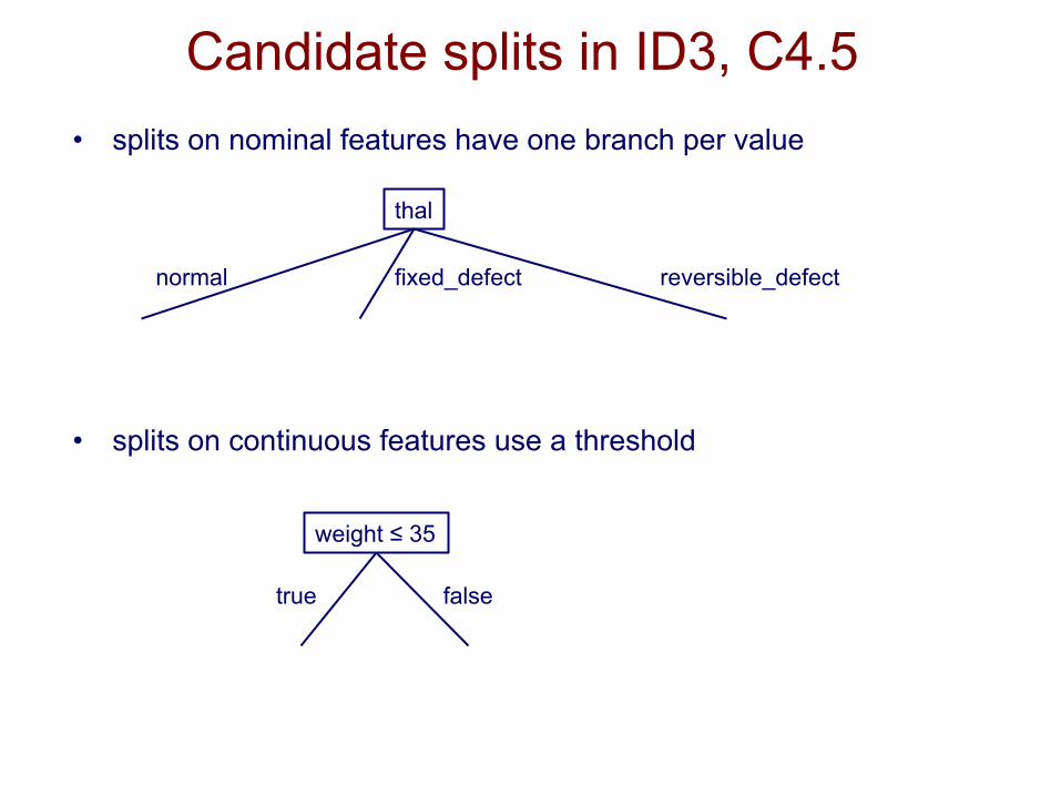
Candidate splits in ID3, C4.5 • splits on nominal features have one branch per value
• splits on continuous features use a threshold
thal
normal fixed_defect reversible_defect
weight ≤ 35
true false

Candidate splits on continuous features
weight ≤ 35
true false
weight
17 35
given a set of training instances D and a specific feature F • sort the values of F in D • evaluate split thresholds in intervals between instances of
different classes
• could use midpoint of each considered interval as the threshold • C4.5 instead picks the largest value of F in the entire training set that
does not exceed the midpoint

Candidate splits on a numeric feature
// Run this subroutine for each numeric feature at each node of DT induction
DetermineCandidateNumericSplits(set of training instances D, feature xi)
C = {} // initialize set of candidate splits for feature xi
S = partition instances in D into sets s1 … sV where the instances in each set have the same value for xi
let vj denote the value of xi for set sj
sort the sets in S using vj as the key for each sj
for each pair of adjacent sets sj, sj+1 in sorted S
if sj and sj+1 contain a pair of instances with different class labels // use midpoints for splits
add candidate split xi ≤ (vj + vj+1)/2 to C
return C

Candidate splits • instead of using k-way splits for k-valued features, could
require binary splits on all discrete features (CART does this)
• Breiman et al. proved for the 2-class case, the optimal binary partition can be found considered only O(k) possibilities instead of O(2k)
thal
normal reversible_defect ∨ fixed_defect
color
red ∨blue green ∨ yellow

Finding the best split
• How should we select the best feature to split on at each step?
• Key hypothesis: the simplest tree that classifies the training examples accurately will work well on previously unseen examples

Occam’s razor
• attributed to 14th century William of Ockham
• “Nunquam ponenda est pluralitis sin necesitate”
• “Entities should not be multiplied beyond necessity”
• “should proceed to simpler theories until simplicity can be traded for greater explanatory power”
• “when you have two competing theories that make exactly the same predictions, the simpler one is the better”

But a thousand years earlier, I said, “We consider it a good principle to explain the phenomena by the simplest hypothesis possible.”

Occam’s razor and decision trees
• there are fewer short models (i.e. small trees) than long ones
• a short model is unlikely to fit the training data well by chance
• a long model is more likely to fit the training data well coincidentally
Why is Occam’s razor a reasonable heuristic for decision tree learning?

Finding the best splits
• Can we return the smallest possible decision tree that accurately classifies the training set?
• Instead, we’ll use an information-theoretic heuristic to greedily choose splits
NO! This is an NP-hard problem [Hyafil & Rivest, Information Processing Letters, 1976]

Information theory background
• consider a problem in which you are using a code to communicate information to a receiver
• example: as bikes go past, you are communicating the manufacturer of each bike

Information theory background
• suppose there are only four types of bikes • we could use the following code
11
10
01
00
• expected number of bits we have to communicate: 2 bits/bike
Trek
Specialized
Cervelo
Serrota
type code

Information theory background • we can do better if the bike types aren’t equiprobable • optimal code uses bits for event with
probability
− log2 P(y)P(y)
1
€
P(Trek) = 0.5P(Specialized) = 0.25P(Cervelo) = 0.125P(Serrota) = 0.125
2 3
3
1
01
001
000
− P(y)log2 P(y)y∈values(Y )∑
Type/probability # bits code
• expected number of bits we have to communicate: 1.75 bits/bike

Entropy • entropy is a measure of uncertainty associated with a
random variable
• defined as the expected number of bits required to communicate the value of the variable
entropy function for binary variable
H (Y ) = − P(y)log2 P(y)
y∈values(Y )∑
P(Y = 1)
H (Y )

Conditional entropy
• What’s the entropy of Y if we condition on some other variable X?
H (Y | X) = P(X = x) H (Y | X = x)
x∈values(X )∑
H (Y | X = x) = − P(Y = y | X = x) log2P(Y = y | X = x)
y∈values(Y )∑
where

Information gain (a.k.a. mutual information)
• choosing splits in ID3: select the split S that most reduces the conditional entropy of Y for training set D
InfoGain(D,S) = HD (Y )− HD (Y | S)
D indicates that we’re calculating probabilities using the specific sample D

Information gain example

Information gain example
Humidity
high normal
D: [3+, 4-]
D: [9+, 5-]
D: [6+, 1-]
• What’s the information gain of splitting on Humidity?
HD (Y ) = −914log2
914"#$
%&'−514log2
514"#$
%&'= 0.940
HD (Y |high) = − 37
log237
"#$
%&'−
47
log247
"#$
%&'
= 0.985
HD (Y |normal) = − 67
log267
"#$
%&'−
17
log217
"#$
%&'
= 0.592
InfoGain(D,Humidity) = HD (Y )− HD (Y |Humidity)
= 0.940 − 714
(0.985)+ 714
0.592( )"#$
%&'
= 0.151

Information gain example
Humidity
high normal
D: [3+, 4-]
D: [9+, 5-]
D: [6+, 1-]
• Is it better to split on Humidity or Wind?
HD (Y |weak) = 0.811
InfoGain(D,Humidity) = 0.940 − 714
(0.985)+ 714
0.592( )"#$
%&'
= 0.151
Wind
weak strong
D: [6+, 2-]
D: [9+, 5-]
D: [3+, 3-]
HD (Y | strong) = 1.0
InfoGain(D,Wind) = 0.940 − 814
(0.811)+ 614
1.0( )"#$
%&'
= 0.048
✔
One limitation of information gain
• information gain is biased towards tests with many outcomes
• e.g. consider a feature that uniquely identifies each training instance – splitting on this feature would result in many
branches, each of which is “pure” (has instances of only one class)
– maximal information gain!

Gain ratio • To address this limitation, C4.5 uses a splitting criterion
called gain ratio
• consider the potential information generated by splitting on S
GainRatio(D,S) = InfoGain(D,S)
SplitInfo(D,S)
SplitInfo(D,S) = −Dk
Dk∈ outcomes(S )∑ log2
Dk
D$
%&
'
()
use this to normalize information gain

Stopping criteria We should form a leaf when
• all of the given subset of instances are of the same class • we’ve exhausted all of the candidate splits
Is there a reason to stop earlier, or to prune back the tree?
How can we assess the accuracy of a tree? • Can we just calculate the fraction of training examples
that are correctly classified?
• Consider a problem domain in which instances are assigned labels at random with P(Y = T) = 0.5
• How accurate would a learned decision tree be on previously unseen instances?
• How accurate would it be on its training set?
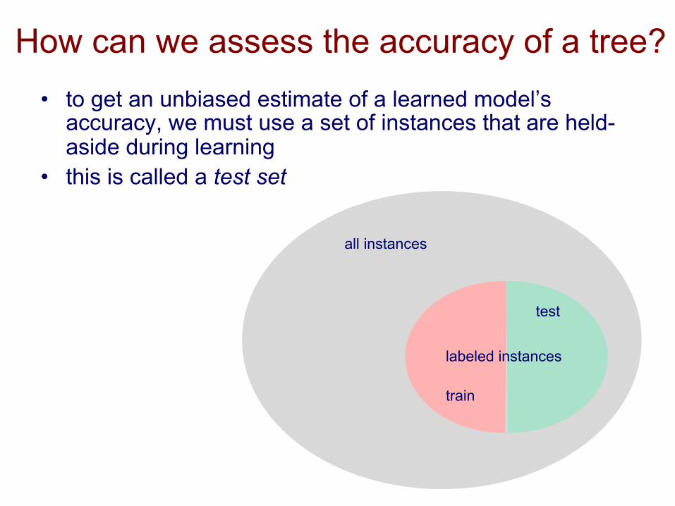
How can we assess the accuracy of a tree? • to get an unbiased estimate of a learned model’s
accuracy, we must use a set of instances that are held-aside during learning
• this is called a test set
all instances
labeled instances
test
train

Overfitting • consider error of model h over
• training data: • entire distribution of data:
• model overfits the training data if there is an
alternative model such that
errorD (h)error(h)
h∈Hh '∈H
error(h) > error(h ')
errorD (h) < errorD (h ')

Overfitting with noisy data suppose
• the target concept is • there is noise in some feature values • we’re given the following training set
Y = X1 ∧ X2
X1 X2 X3 X4 X5 … Y T T T T T … T T T F F T … T T F T T F … T T F F T F … F T F T F F … F F T T F T … F
noisy value
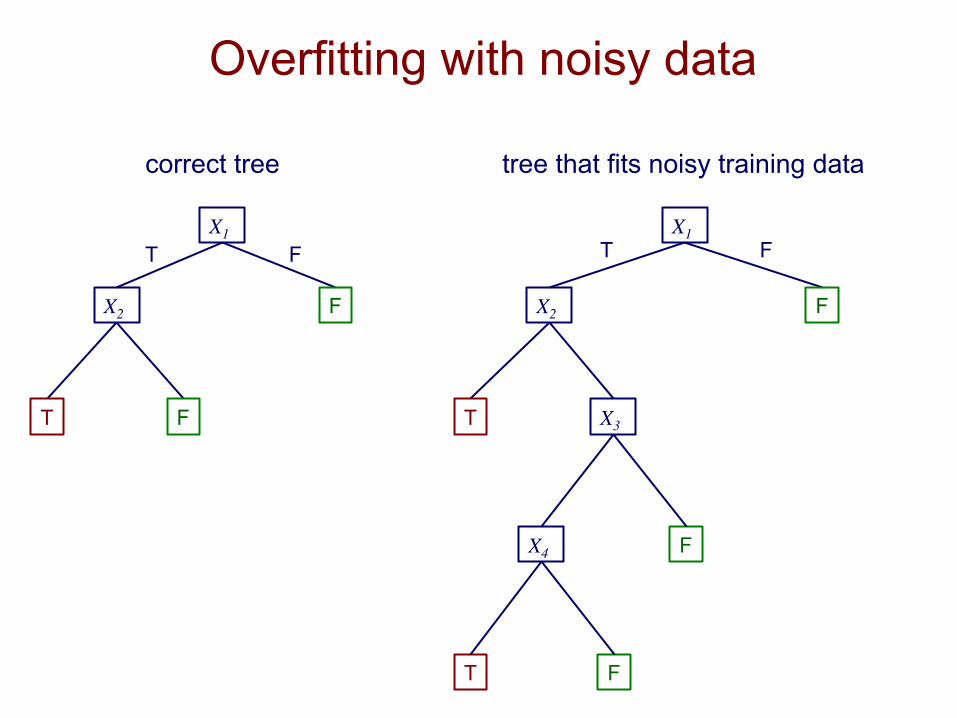
Overfitting with noisy data
X1
X2
T F
X3 T
F
F
F
X4
T
X1
X2
T F
T F
F
correct tree tree that fits noisy training data
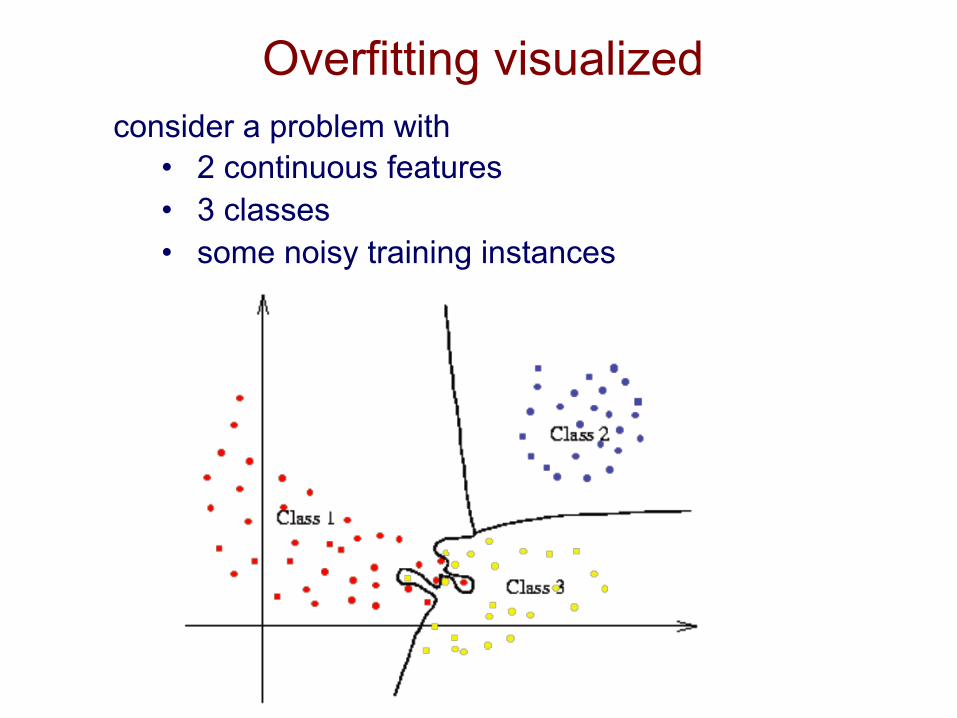
Overfitting visualized consider a problem with
• 2 continuous features • 3 classes • some noisy training instances

Overfitting with noise-free data suppose
• the target concept is • P(X3 = T) = 0.5 for both classes • P(Y = T) = 0.67 • we’re given the following training set
Y = X1 ∧ X2
X1 X2 X3 X4 X5 … Y T T T T T … T T T T F T … T T T T T F … T T F F T F … F F T F F T … F

Overfitting with noise-free data
X3
T F
T F
T
training set accuracy
test set accuracy
100%
66% 66%
50%
• because the training set is a limited sample, there might be (combinations of) features that are correlated with the target concept by chance

Overfitting in decision trees

Avoiding overfitting in DT learning
two general strategies to avoid overfitting 1. early stopping: stop if further splitting not justified by
a statistical test • Quinlan’s original approach in ID3
2. post-pruning: grow a large tree, then prune back some nodes • more robust to myopia of greedy tree learning

Pruning in ID3, C4.5
1. split given data into training and tuning (validation) sets
2. grow a complete tree 3. do until further pruning is harmful
• evaluate impact on tuning-set accuracy of pruning each node
• greedily remove the one that most improves tuning-set accuracy

Tuning sets • a tuning set (a.k.a. validation set) is a subset of the training set
that is held aside • not used for primary training process (e.g. tree growing) • but used to select among models (e.g. trees pruned to
varying degrees)
all instances
labeled instances
test train
tuning

Regression trees
X5 > 10
X3
X2 > 2.1 Y=5
Y=24 Y=3.5
Y=3.2
• in a regression tree, leaves have functions that predict numeric values instead of class labels
• the form of these functions depends on the method • CART uses constants: regression trees • some methods use linear functions: model trees
X5 > 10
X3
X2 > 2.1 Y=2X4+5
Y=3X4+X6
Y=3.2
Y=1

Regression trees in CART
• CART does least squares regression which tries to minimize
= yi − yi( )2
i∈L∑
L∈leaves∑
yi − yi( )2i=1
D
∑
target value for ith training instance
value predicted by tree for ith training instance (average valueof y for training instances reaching the leaf)
• at each internal node, CART chooses the split that most reduces this quantity

m-of-n splits • a few DT algorithms have used m-of-n splits [Murphy & Pazzani ‘91] • each split is constructed using a heuristic search process • this can result in smaller, easier to comprehend trees
test is satisfied if 5 of 10 conditions are true
tree for exchange rate prediction [Craven & Shavlik, 1997]

Searching for m-of-n splits m-of-n splits are found via a hill-climbing search
• initial state: best 1-of-1 (ordinary) binary split
• evaluation function: information gain
• operators:
m-of-n è m-of-(n+1)
m-of-n è (m+1)-of-(n+1)
1 of { X1=T, X3=F } è 1 of { X1=T, X3=F, X7=T }
1 of { X1=T, X3=F } è 2 of { X1=T, X3=F, X7=T }

Lookahead
• most DT learning methods use a hill-climbing search • a limitation of this approach is myopia: an important feature may
not appear to be informative until used in conjunction with other features
• can potentially alleviate this limitation by using a lookahead search [Norton ‘89; Murphy & Salzberg ‘95]
• empirically, often doesn’t improve accuracy or tree size

Choosing best split in ordinary DT learning
OrdinaryFindBestSplit(set of training instances D, set of candidate splits C)
maxgain = -∞
for each split S in C
gain = InfoGain(D, S)
if gain > maxgain
maxgain = gain
Sbest = S
return Sbest

Choosing best split with lookahead (part 1)
LookaheadFindBestSplit(set of training instances D, set of candidate splits C)
maxgain = -∞
for each split S in C
gain = EvaluateSplit(D, C, S)
if gain > maxgain
maxgain = gain
Sbest = S
return Sbest

Choosing best split with lookahead (part 2)
EvaluateSplit(D, C, S)
if a split on S separates instances by class (i.e. )
// no need to split further
return
else
for outcomes of S // let’s assume binary splits
// see what the splits at the next level would be
Dk = subset of instances that have outcome k
Sk = OrdinaryFindBestSplit(Dk, C – S)
// return information gain that would result from this 2-level subtree
return
HD (Y | S) = 0
k ∈ 1, 2{ }
HD (Y )− HD (Y | S,S1,S2 )
HD (Y )− HD (Y | S)

Calculating information gain with lookahead
Humidity
Wind Temperature
D: [12-, 11+]
D: [6-, 8+] D: [6-, 3+]
D: [2-, 3+] D: [4-, 5+] D: [2-, 2+] D: [4-, 1+]
Suppose that when considering Humidity as a split, we find that Wind and Temperature are the best features to split on at the next level
high normal
strong weak high low
We can assess value of choosing Humidity as our split by HD(Y) - HD(Y | Humidity, Wind, Temperature)

Calculating information gain with lookahead
HD (Y | Humidity,Wind,Temperature) = 523HD (Y | Humidity = high,Wind = strong)+
923HD (Y | Humidity = high,Wind = weak)+
423HD (Y | Humidity = low,Temperature = high)+
523HD (Y | Humidity = low,Temperature = low)
HD (Y | Humidity = high,Wind = strong) = − 25
log 25
"#$
%&'−
35
log 35
"#$
%&'
Using the tree from the previous slide:

Comments on decision tree learning
• widely used approach • many variations • fast in practice • provides humanly comprehensible models when
trees not too big • insensitive to monotone transformations of numeric
features • standard methods learn axis-parallel hypotheses* • standard methods not suited to on-line setting* • usually not among most accurate learning methods
* although variants exist that are exceptions to this