1

Decoding EEG Signals Using Deep Neural Networks:

A Basis for Sleep Analysis

Alana Jaskir, ‘17, Department of Computer Science

Fall Junior Independent Project 2015

Advisor: Ken Norman, Professor of Psychology and the Princeton Neuroscience

Institute

Introduction

This work falls under the larger study of sleep’s role in determining the fate of individual

memories currently being conducted by Professor Norman, graduate student Luis

Piloto, and other researchers. The goal of this independent work is to investigate deep

neural network (DNN) designs and understand their effectiveness in decoding

electroencephalography (EEG) signals for cognitive categorical information.

Related Work

Many invasive electrode rodent studies have helped to illuminate elements of the

phenomenon of replay, or the reactivation of previously stored information, during sleep

that aids in memory consolidation1,2. In humans, the benefits of sleep have been shown

on a behavioral level and the analysis of neural mechanics in healthy subjects are

limited to noninvasive forms of measurement such as functional magnetic resonance

imaging (fMRI) and EEG3,4. Identifying the exact temporal moments of these replayed

1 Ego-Stengel, V. & Wilson, M. A. Disruption of ripple-associated hippocampal activity during rest impairs spatial learning in the rat. Hippocampus 20, 1–10 (2010). 2 Pavlides, C. & Winson, J. Influences of hippocampal place cell firing in the awake state on the activity of these cells during subsequent sleep episodes. J. Neurosci. 9, 2907–18 (1989). 3 Rauchs, G., Feyers, D., Landeau, B., Bastin, C., Luxen, A., Maquet, P., Collette, F. Sleep contributes to the strengthening of some memories over others, depending on hippocampal activity at learning. J. Neurosci. 31, 2563–8 (2011).

2

memories and relevant features of the signal is difficult. A previous study successfully

identified spontaneous stimulus-specific intrasubject replay neural activity using fMRI

analysis using multivariate pattern classification analysis (MVPA). However, fMRI has a

lower temporal resolution than that of electrode as well as EEG studies and it is an

indirect measurement of neural activity, a critique the researchers themselves specify5.

Study Background

In the study whose data analysis appears in this paper, subjects were first exposed to

images of faces, places, objects, scrambled faces, and scrambled places. For each

image they then learned an associated unique tone and later location on the screen.

During the nap, the researchers played half the sounds, a technique called Targeted

Memory Reactivation, to encourage replay of the associated face or scene during

stages of slow-wave sleep. EEG signals were recorded during the training and nap

stages of the experiment. The played sounds offer a benchmark for when these replays

occur during sleep, but do not offer concrete evidence for the occurrence of replay. For

this preliminary study, the lab has previously analyzed the sleep data for replay and

classified some sleep data significantly above chance using multi-voxel pattern analysis

(MVPA) 6. The effectiveness of DNNs in this sleep analysis, as well as understanding

replay through the lens of DNNs, is the larger objective of this project.

4 Cox, R., Hofman, W. F. & Talamini, L. M. Involvement of spindles in memory consolidation is slow wave sleep-specific. Learn. Mem. 19, 264–7 (2012). 5 Deuker, L., Olligs, J., Fell, J., Kranz, T. A., Mormann, F., Montag, C., Reuter, M., Elger, C. E., Axmacher, N. Memory consolidation by replay of stimulus-specific neural activity. J. Neurosci. 33, 19373–83 (2013). 6 Antony, J. W., Piloto, L. R., Paller, K. A., & Norman, K. A. (2014). Using multivariate pattern analysis to investigate memory reactivation during sleep. Poster presented at the Society for Neuroscience Annual Meeting, Washington, DC.

3

Approach

Deep neural networks have applications in a wealth of fields, including natural language

processing7, computer vision8, and speech recognition9. Their power of classification,

ability to compute high-level abstractions of data, and insight into hidden relationship

among inputs make it an ideal tool for analyzing and identifying moments of replay. In

the field of neuroscience, DNNs have been recently used for fMRI analysis10. For EEG

analysis, DNNs have been used in identifying epileptic seizures11 as well as in Brain

Computer Interaction for emotion detection12 and brain state classification13. A study

by Stober et al. offer a useful technique to identify stable features across subject trials to

aid networks and help autoencoders feature select14. In sleep studies, DNNs have been

applied to EEG to identify different sleep stages15, which involves changes in holistic

neuron firing rates rather than specific patterns, and as of now the use of DNNs to

extract categorical cognitive sleep information is as of now a novel approach. For this

semester, the focus has been to classify categorical data - a face versus a place - in the 7 Collobert, R. & Weston, J. A unified architecture for natural language processing: deep neural networks with multitask learning. Proc. Twenty-fifth Int. Conf. Mach. Learn. 20, 160–7 (2008). 8 Krizhevsky, A., Sutskever, I. & Hinton, G. E. ImageNet classification with deep convolutional neural networks. Adv. Neural Inf. Process. Syst. 1–9 (2012). 9 Graves, A., Mohamed, A. & Hinton, G. Speech recognition with deep recurrent neural networks. IEEE Int. Conf. Acoust. Speech Signal Process. (2013). doi:10.1109/ICASSP.2013.6638947 10 Plis, S. M., Hjelm, D. R., Salakhutdinov, R., Allen, E. A., Bockholt, H. J., Long, J. D., Johnson, H., Paulsen, J., Turner, J., Calhoun, V. D. Deep learning for neuroimaging: A validation study. Front. Neurosci. 8, 229 (2014). 11 Srinivasan, V.; Eswaran, C.; Sriraam, N., Approximate Entropy-Based Epileptic EEG Detection Using Artificial Neural Networks, in Information Technology in Biomedicine, IEEE Transactions on , 11.3, 288-295, 2007 doi: 10.1109/TITB.2006.884369 12 Jirayucharoensak, S., Pan-Ngum, S., and Israsena, P. EEG-Based Emotion Recognition Using Deep Learning Network with Principal Component Based Covariate Shift Adaptation. The Scientific World Journal, 2014. 13 Cecotti, H. and Graser, A. Convolutional Neural Network with embedded Fourier Transform for ̈EEG classification. In 19th International Conference on Pattern Recognition (ICPR), pp. 1–4, 2008. 14 Stober, S., Sternin, A., Owen, A. M., & Grahn, J. A. Deep Feature Learning for EEG Recordings. Under review for International Conference on Learning Representations. (2016) 15 Längkvist, M., Karlsson, L. & Loutfi, A. Sleep stage classification using unsupervised feature learning. Adv. Artif. Neural Syst. 2012, 1–9 (2012).

4

awake initial exposure phase of the previously described experiment to understand the

performance of DNNs on decoding EEG data as a baseline for future applications to

sleep analysis.

Implementation

Tools

The two major tools used for this project’s implementation are Torch and MATLAB.

Torch, the computing framework and machine learning library built on Lua, is used by

Google Deepmind16, Facebook’s AI research group17, and other companies. Its use in

this project involves: categorizing, restructuring, and dividing data into three data sets -

training, validation, and testing; network development through creation, training, and

validation; and logging progress. MATLAB uses the data logged to analyze and

visualize network performance.

Dataset

The data analyzed comes from the initial exposure phase of the above-mentioned

experiment from 7633 trials across 33 subjects. The ERP (event-related potential) from

the EEG cap was measured from stimulus onset to 250 time-steps post-stimulus. The

interval before time steps is four milliseconds. The EEG cap consisted of 64 channels.

16 Braun, Mikio L. "What Is Going on with DeepMind and Google?" Marginally Interesting. N.p., 28 Jan. 2014. Web. 17 Piatetsky, Gregory. "Interview with Yann LeCun, Deep Learning Expert, Director of Facebook AI Lab." KDnuggets Analytics Big Data Data Mining and Data Science. N.p., 20 Feb. 2014. Web.

5

Process Overview

Below is a general overview of the logic flow of the code followed by more in depth

details.

• Data Processing

o Time Bin separation

o Category Separation

o Normalization

• Network creation

o Network Design

o Parameters

• Training

o Mini-batch training

o Validation analysis

o Log progress

Data Processing

Initially, it was attempted to train a classifier over all time points over all trials. However,

the process quickly reached the allowed limit on the cluster. This prompted both a

revision of a significant portion of the code to make it more memory efficient and the

need to divide data into time bins. Therefore classifiers were trained on sections of fifty

time steps, with Classifier 1 being trained on time steps 1 to 50 (4-200ms), Classifier 2

on time steps 51 to 100 (204-400ms), Classifier 3 on time steps 101 to 150 (404-

6

600ms), Classifier 4 on time steps 151 to 200 (604-800ms), and finally Classifier 5 on

time steps 201 to 250 (804-1000ms).

Each classifier was trained across all subjects. 75% of the data was used for the

training data set, 15% was used for the validation test during testing, and the remaining

10% is reserved as the test set to be used for final evaluation of a network. All data was

separated into respective categories - faces, places, objects, scrambled faces, and

scrambled places - and then randomly divided into three groups with sizes proportioned

75%, 15%, and 10% to the number of trials in that category and placed in the respective

dataset.

All data was normalized with the mean and standard deviation of the training set.

Network Creation

For simplicity, this project used feed-forward networks with hidden layers of equal

number of hidden units. The three major parameters modified were the number of

hidden layers, number of hidden units, and learning rate of the network. See Figure 1

for a diagram of the network layout.

The network, as seen in Figure 1, fluctuates the three major architecture parameters in

addition to the optimizer. In later networks, the optimizer Adam18 was used

experimentally to test its benefits. Stochastic gradient descent was the main optimizer

18 Kingma, D. P. & Ba, J. L. Adam: A Method for Stochastic Optimization. International Conference on Learning Representations. (2015)

7

used in this study and is commonly used in neural network training. The full list of

parameter combinations can be found in Table 1.

FIGURE 1: Network Diagram

Stable aspects of the network design include the activation functions and loss function.

The value of each node input node is multiplied by the respective parameter weight, w,

that connects it to a node in the next layer. All such products are linearly combined for

each node and then an activation function is applied to this sum. The two activation

functions used are the rectifier and log softmax which have the following definitions:

Rectifier Function: 𝑓(𝑖𝑛𝑝𝑢𝑡)  =  𝑚𝑎𝑥(0, 𝑖𝑛𝑝𝑢𝑡)

Log Softmax Function: 𝑓!(𝑥)  =  𝑙𝑜𝑔 !"#(!!)!

    ,𝑤ℎ𝑒𝑟𝑒  𝑎 = 𝑒𝑥𝑝(𝑥!)!"!#$%!!!    

8

Rectified linear units (ReLU), as well as tanh and sigmoid functions, are common

activation functions. ReLU tend to be faster and do not suffer from the vanishing

gradient problem as the other functions do. Log Softmax is a way to enforce outputs of

the network to lie between zero and one and sum to one, producing a measure of

probability of a given input belonging to a category. The Class Negative Log Likelihood

takes the negative of these log probabilities of each class for the loss, which is then

backpropagated. This creates a five-way classifier network.

As the number of input features going into the system is equivalent to the number of

time steps in each bin times the number of EEG channels (for a total of 3200 features)

and the number of trials is 7633, it is important to limit the complexity of the network (the

number of parameter weights being learned) to avoid overfitting relative to these

dimensions. Overfitting occurs when the network becomes too specialized to the

training set and Is unable to accurately generalize to novel cases. This can happen

when the network is too complex and attempts to describe the data using too

complicated of a function, when it is too simple of a network, or from excessive

overtraining of the network. The sweeping parameters tested in the first set of networks

unfortunately started with a larger range of parameters that led quickly to overfitting.

Rather than starting with complexity and then decreasing the complexity with time as

originally done here, it is better to instead start with simple networks and increase

complexity as needed.

9

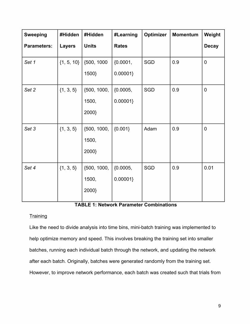
Sweeping

Parameters:

#Hidden

Layers

#Hidden

Units

#Learning

Rates

Optimizer Momentum Weight

Decay

Set 1 {1, 5, 10} {500, 1000

1500}

{0.0001,

0.00001}

SGD 0.9 0

Set 2 {1, 3, 5} {500, 1000,

1500,

2000}

{0.0005,

0.00001}

SGD 0.9 0

Set 3 {1, 3, 5} {500, 1000,

1500,

2000}

{0.001} Adam 0.9 0

Set 4 {1, 3, 5} {500, 1000,

1500,

2000}

{0.0005,

0.00001}

SGD 0.9 0.01

TABLE 1: Network Parameter Combinations

Training

Like the need to divide analysis into time bins, mini-batch training was implemented to

help optimize memory and speed. This involves breaking the training set into smaller

batches, running each individual batch through the network, and updating the network

after each batch. Originally, batches were generated randomly from the training set.

However, to improve network performance, each batch was created such that trials from

10

the same category were equally distributed among each batch. This project used 500

trials for each mini-batch.

Once all batches went through the network, the validation set then was ran through the

network without backpropagating its errors. This is used as a benchmark for network

generalization to novel trials.

This process - mini-batch training and validation set verification - constitutes one

iteration of training. Networks were run for a maximum of 10,000 such iterations. At

each iteration step, the network loss, the confusion matrix of what each trial the network

classified in comparison to its true label, the precision of each category, and the

average precision of both the training and validation trials were tracked and logged.

Results

The specific categories of interest are the classification abilities of the face and place

trials, though overall network performance is necessary to assess network abilities.

Initially the validation accuracy, or the percent of correct classification, had been used

as a measurement of network performance. However, this can be misleading and hide

inherent biases of the network, for example a network can score quite well in one

category but only because it always chooses that category with a high probability.

11

For this project, the following calculation was used as a measure of performance for a

given category, c.

true positivesc Performancec = .

#trialsc + false positivesc

This measurement has some resistance to network biases and the average

performance over classes is resistant to large differences in number of trials amongst

categories.

Another form of performance measurement is the area under the receiver operating

characteristic (ROC) curve, which is a plot of true positive rate against false positive rate

with varying threshold values. While this performance measurement is preferred, time

restraints hindered the completion of this analysis code. As the above performance

calculation had been built into Torch’s Confusion Matrix data structure, it was used as a

benchmark for analysis within this project. ROC will be implemented for further studies.

While the Set 2 parameters were run on all time bins, the variations of other parameters

was run solely on Classifier 2 for time steps 51 thorough 200. This was because signal

is not expected within the first 150 seconds or so and also to narrow the focus of

experimentation. For the purpose of this project report, only data from Classifier 2 will

be discussed.

12

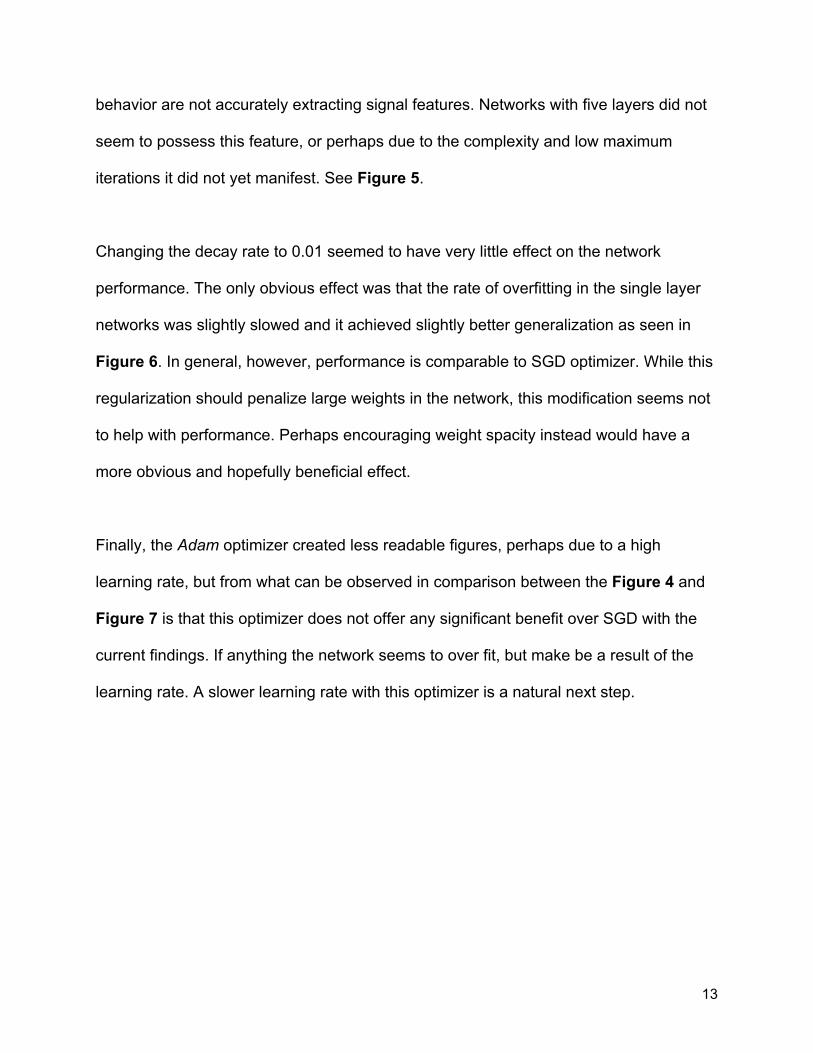
As previously mentioned, the extremely complicated networks of Set 1, that is networks

with 10 hidden layers, led to dramatic overfitting and poor performance as seen in

Figure 2. These graphs use percent correct, which is not sensitive to network biases

but had previously been used before code modification. However, upon analyzing the

respective confusion matrix, the network had a strong internal bias of choosing only one

category regardless of input. The train loss (not shown) with this networks also

surprisingly increased over time while the valid had a U shape as the network most

likely was using too sophisticated of a measurement to differentiate between categories.

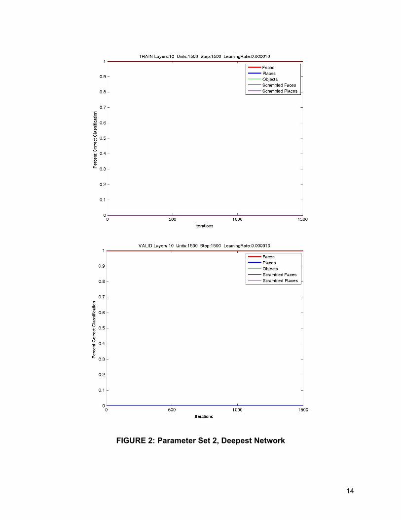
After eliminating the larger networks, Set 2 parameters were ran on the partition of

second time steps. Networks with more moderate depth (with 3-5 hidden layers) and

smaller height (500 or 1000 units per layer) had better performance than the single layer

that often lead to overfitting of the training data as evident by Figure 3. That being said,

the precision for the face and place categories, which are the ones of interest, still did

not perform well though it avoided the overfitting issue of the single layer. See Figure

4.

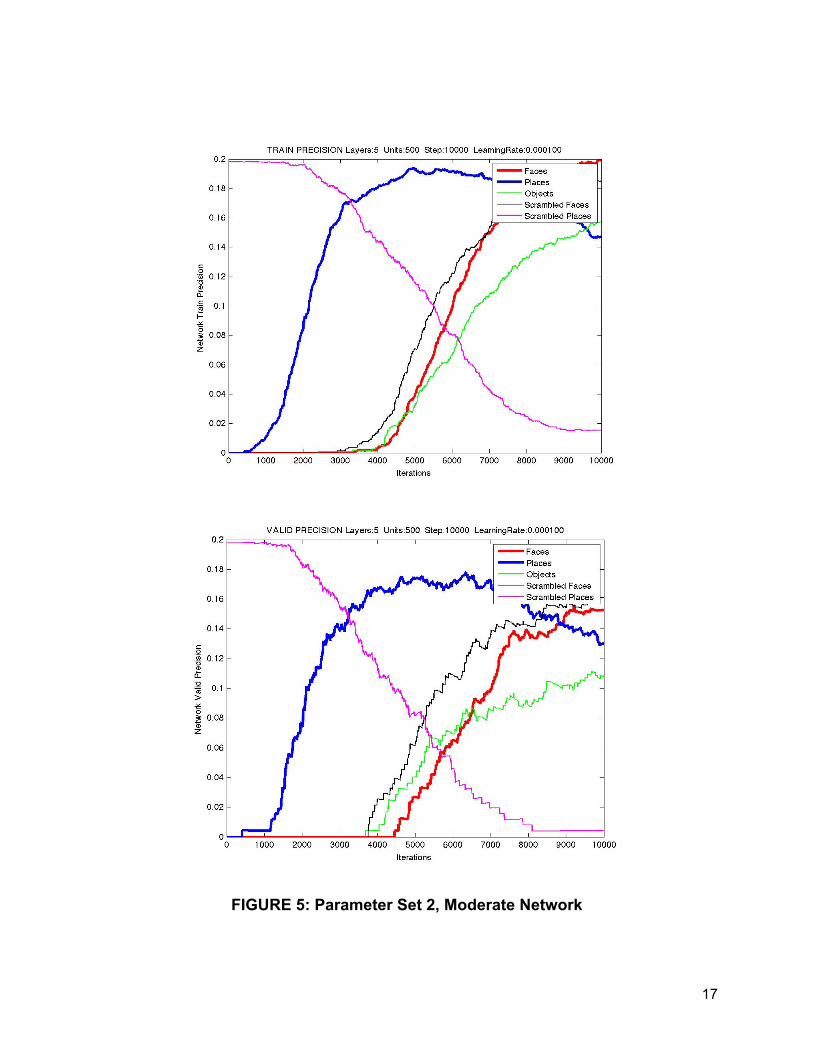
An interesting trend appeared during this set of parameters with 3 layers where often

the scrambled faces and scrambled places yielded better training and validation

precision than the desired faces and places category. According to the confusion

matrices (data not shown), the network categorized a disproportionate amount of trials

as either of the scrambled categories. Since these theoretically should not have any

distinguishable pattern or noise, this may mean that those networks that exhibit such a

13

behavior are not accurately extracting signal features. Networks with five layers did not

seem to possess this feature, or perhaps due to the complexity and low maximum

iterations it did not yet manifest. See Figure 5.

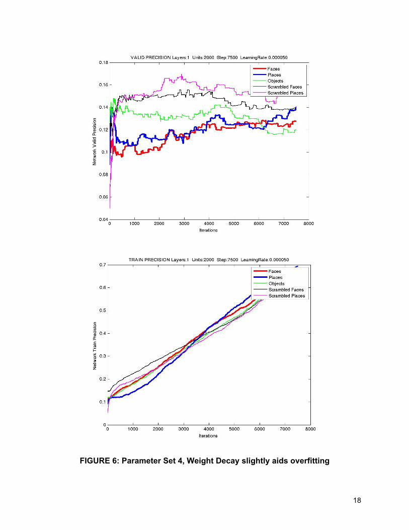
Changing the decay rate to 0.01 seemed to have very little effect on the network

performance. The only obvious effect was that the rate of overfitting in the single layer

networks was slightly slowed and it achieved slightly better generalization as seen in

Figure 6. In general, however, performance is comparable to SGD optimizer. While this

regularization should penalize large weights in the network, this modification seems not

to help with performance. Perhaps encouraging weight spacity instead would have a

more obvious and hopefully beneficial effect.

Finally, the Adam optimizer created less readable figures, perhaps due to a high

learning rate, but from what can be observed in comparison between the Figure 4 and

Figure 7 is that this optimizer does not offer any significant benefit over SGD with the

current findings. If anything the network seems to over fit, but make be a result of the

learning rate. A slower learning rate with this optimizer is a natural next step.

14

FIGURE 2: Parameter Set 2, Deepest Network

15

FIGURE 3: Parameter Set 2, Deepest Network

16

FIGURE 4: Parameter Set 2, Moderate Network

17

FIGURE 5: Parameter Set 2, Moderate Network

18

FIGURE 6: Parameter Set 4, Weight Decay slightly aids overfitting

19

FIGURE 7: Parameter Set 3, Adam optimizer

20

Conclusions, Further Steps, and Commentary

While no final network achieved a satisfactory level of categorization, the current work

sets a strong foundation for future steps in the coming semester as well as offers insight

into the capabilities and limitations of deep neural networks in decoding EEG data. This

insight is necessary to understand before sleep analysis, where greater uncertainty

exists in the data.

Further Steps

These are the current proposed steps of exploration for the coming semester:

Simulated Data on network

As what classifies as a “face” trial and a “place” trial is not distinguishable by humans by

looking at raw EEG data, it is difficult to verify if the network is performing accurate

feature extraction. A good test is to simulate mock data whose characteristics are

known and use this to understand the networks performance.

Implementing ROC analysis

As discussed before, this is a more conventional measurement of network performance

and should be implemented for evaluating future networks.

Other Classifier Time Bins

These analyses only focused on Classifier 2. Exploration for the other classifier time

bins that may also hold signal is another area to expand.

21

Intrasubject analysis

While it would be preferable to create a classifier that not only applies to novel trials but

also novel subjects, the type of across-subject classification in this paper comes with

added difficulties of encoding variations between subjects and other subject-specific

characteristics. An easier classifier may be one trained internally for a subject.

Alternatively, the previously mentioned paper by Stober et al. may offer insight in how to

aid the network with feature extraction.

Architecture

Rather than having hidden layers with uniform height, trickling down the height may

simplify the network and assist with classification. Alternatively, other types of neural

networks may offer better performance, such as convolutional neural networks.

However, for the moment, focus should remain on the above few goals.

Setbacks, Resolutions, and Lessons

Technical Issues

As specified earlier, memory limitations caused a large number of implementation

changes about halfway through the project’s duration. The described modifications had

been made to training and time-bin division to solve this issue, as well as other coding

inefficiencies.

Other technical limitations and issues also arose during the project’s progress. Some of

the later networks started producing unusable data due to some form of file corruption,

22

which was not realized until several days of running the network. The issue had thought

to have been resolved, another long training session ran, and the data again had been

unusable. This unfortunately caused a major setback in network analysis and

generation. After tracing through the code, and modifying some of the new mini-batch

implementation, the networks began producing useable data again though the exact

issue is still not known.

Establishing a Foundation

A large portion of time had been spent in the initial research phase of this project as well

as learning the unfamiliar Torch framework and Lua syntax. It was difficult to

educationally approach the network design without having a strong prior conceptual

understanding of the mathematical background, which meant time was spent analyzing

and implementing smaller toy projects to consolidate ideas. The learning process also

did not stop once the main project implementation began, as it opened new questions

and educational opportunities that, while took time, aided to my overall conception and

understanding of neural networks and intuition. These include things such as basic

syntactical questions, lessons in avoiding overfitting, and proper analysis methods.

Thankfully the bulk of the initial learning hump has been climbed, so while progress

moved much more slowly than anticipated this semester a stronger foundation exists for

future studies.

23

Acknowledgments

An enormous thank you to both Professor Norman and Luis Piloto for their guidance

and support during this project.

Honor Code

I pledge my honor that this project represents my own work in accordance with

University regulations.

Alana Jaskir