dedicated to - eprintseprints.kfupm.edu.sa/136296/1/design_of_an_lte_antenna_for_mobile... · 4.4...
TRANSCRIPT


Dedicated to
My Parents
Whose Prayers and Perseverance led to this accomplishment

ii
ACKNOWLEDGEMENTS
In the name of Allah, the Most Gracious and the Most Merciful
All praises and glory be to Allah (SWT) for blessing me with opportunities abound and
showering upon me his mercy and guidance all through the life. I pray that He continues the
same the rest of my life. And may his peace and blessings of Allah be upon Prophet Muhammad,
a guidance and inspiration to our lives.
I would like to thank my supervisors, Dr. Sheikh Sharif Iqbal and Dr. Mohammad S.
Sharawi for their guidance and expertise throughout this thesis. There were always there when I
needed them, and even with their tight schedule, they have always found time for me. I am
extremely grateful to them for their prompt replies and their numerous proofreads. I am also very
grateful to my thesis committee members, Dr. Mahmoud M. Dawoud, Dr. Husain M. Masoudi
and Dr. Mohammad A. Alsunaidi, for their care, cooperation and constructive advice.
Special thanks to my colleagues and friends for their encouragements and various help
that they provided throughout my graduate studies at KFUPM. I would like to give my special
thanks to my parents, brother and my sister for their support, patience and love. Without their
encouragement, motivation and understanding it would have been impossible for me to complete
this work.

iii
Table of Contents
ACKNOWLEDGEMENTS ............................................................................................................ ii
LIST OF TABLES ......................................................................................................................... vi
LIST OF FIGURES ...................................................................................................................... vii
THESIS ABSTRACT .................................................................................................................... xi
THESIS ABSTRACT (ARABIC) ............................................................................................... xiii
CHAPTER 1 ................................................................................................................................... 1
INTRODUCTION .......................................................................................................................... 1
1.1 Review of Mobile Communication Standard ................................................................... 1
1.1.1 Introduction ............................................................................................................... 2
1.1.2 The first mobile generations (1G to 2.5G) ................................................................ 3
1.1.3 Third mobile generation networks (3G) ................................................................... 3
1.1.4 Future mobile generation networks (4G) .................................................................. 6
1.2 Long Term Evolution (LTE) ............................................................................................ 7
1.2.1 What is LTE? .................................................................................................................. 8
1.2.2 LTE Bands ...................................................................................................................... 9
1.2.4 Performance Goals for LTE ......................................................................................... 11
1.2.5 Enabling Technologies in LTE ............................................................................... 13
1.2.6 LTE Antennas ............................................................................................................... 19

iv
1.3 Thesis Motivation ........................................................................................................... 21
1.4 Thesis Objectives ........................................................................................................... 22
1.5 Thesis Overview ............................................................................................................. 23
CHAPTER 2 ................................................................................................................................. 24
LITERATURE REVIEW ............................................................................................................. 24
2.1 Introduction ......................................................................................................................... 24
2.2 Printed Antenna for Mobile Devices ................................................................................... 27
2.2.1 Antenna Basics ............................................................................................................. 28
2.2.2 Printed Antennas........................................................................................................... 35
2.3 Electrically Small Antenna.................................................................................................. 41
2.3.1 Fundamental Limitations .............................................................................................. 41
2.3.2 Limit on Radiation Efficiency ...................................................................................... 42
2.4 MIMO Antenna ................................................................................................................... 44
2.4.1 Multiple Antennas ........................................................................................................ 45
2.4.2 Antenna Array .............................................................................................................. 52
CHAPTER 3 ................................................................................................................................. 56
Design of an Electrically Small Antenna ...................................................................................... 56
3.1 Empirical Design of a Meander Line Antenna.................................................................... 56
3.2 Design of an Electrical Small Antenna .......................................................................... 60
3.3 Parameters Variation ...................................................................................................... 68

v
3.3.1 Dielectric Permittivity (𝜺𝒓) ..................................................................................... 68
3.3.2 Spacing Between MLA Arms ................................................................................. 69
3.3.3 Width of the Meander Line Antenna ............................................................................ 71
3.3.4 Length of the Meander Line Antenna ........................................................................... 73
3.3.5 Width of the Matching Line ......................................................................................... 75
3.3.6 Length of the Ground Plane .......................................................................................... 77
3.4 Planar Inverted F Antenna (PIFA) ................................................................................. 79
3.5 Conclusion ...................................................................................................................... 82
CHAPTER 4 ................................................................................................................................. 83
Design of a MIMO Antenna System ............................................................................................ 83
4.1 Design of a 2 Element MIMO Antenna System ................................................................. 83
4.2 Improving Isolation between Antenna Elements ................................................................ 89
4.3 Design of Array Feeder ..................................................................................................... 100
4.4 Design of a Two-Element MIMO Antenna Array ............................................................ 101
4.5 Conclusion ......................................................................................................................... 103
CHAPTER 5 ............................................................................................................................... 104
EXPERIMENTAL RESULTS.................................................................................................... 104
5.1 Experimental Setup ........................................................................................................... 104
5.2 Single LTE Antenna .......................................................................................................... 105
5.3 MIMO Antenna System .................................................................................................... 112

vi
5.4 Conclusion ......................................................................................................................... 120
CHAPTER 6 ............................................................................................................................... 121
CONCLUSION ........................................................................................................................... 121
6.1 Contribution ...................................................................................................................... 121
6.2 Future Work ...................................................................................................................... 122
Appendix A ................................................................................................................................. 123
Experimental Process .............................................................................................................. 123
Network Analyzer Calibration ............................................................................................. 123
Appendix B ................................................................................................................................. 126
Simulator Software Used ........................................................................................................ 126
B.1 What is HFSS? .............................................................................................................. 126
B.2 Error Analysis ............................................................................................................... 127
B.3 Ansoft HFSS Tutorial: Dipole Antenna ........................................................................ 128
Bibliography ............................................................................................................................... 140
Vitae ............................................................................................................................................ 150
LIST OF TABLES
Table 1: Transport Technologies [4], [5] ....................................................................................................................... 4
Table 2: LTE FDD Frequency Bands and Channel Numbers [5] ................................................................................ 10

vii
Table 3: LTE Performance Requirements [9].............................................................................................................. 11
Table 5: Dielectric Permittivity Effect on the Design ................................................................................................. 68
Table 6: PIFA Specifications ....................................................................................................................................... 80
Table 7: Differences between MLA & PIFA............................................................................................................... 82
Table 8: Summary for the Four Cases of MIMO Antenna .......................................................................................... 86
Table 9: Specification for the Two Element MIMO Antenna ..................................................................................... 97
Table 10: Dimensions of the two way Power Divider of figure 4.5 (a) ..................................................................... 101
Table 11: Simulated and Experimental Results for Single MLA Antenna ................................................................ 107
LIST OF FIGURES
Figure 1: The Evolution of Wireless Communication Standards [7] ............................................................................. 7
Figure 2: MIMO System Diagram ............................................................................................................................... 18
Figure 3: LTE Frequency Spectrum Auctions [7] ....................................................................................................... 20
Figure 4: Basic rectangular microstrip patch antenna construction ............................................................................. 37
Figure 5: The Fundamental Section of the Meander Line Antenna ............................................................................. 39
Figure 6: Planar Inverted F Antenna ........................................................................................................................... 40
Figure 7: Equivalent circuits of a magnetic and electric dipole ................................................................................... 44
Figure 8: HFSS Model for a MLA Based on Empirical Equations ............................................................................. 58
Figure 9: Reflection Coefficient of the Empirical Design ........................................................................................... 59
Figure 10: Sphere enclosing an electrically small radiating element ........................................................................... 60
Figure 11: Schematic Diagram of the Proposed Design .............................................................................................. 62
Figure 12: Reflection Coefficient for the Designed MLA ........................................................................................... 63
Figure 13: MLA (a) 3D Radiation Pattern (b) Azimuth (theta=900) Plane Pattern and (c) Elevation (phi=90
0) ......... 64
Figure 14: MLA HFSS Model ..................................................................................................................................... 65

viii
Figure 15: Effect of Spacing on Center Frequency ..................................................................................................... 70
Figure 16: Effect of Spacing on Reflection Coefficient .............................................................................................. 70
Figure 17: Effect of Spacing on Bandwidth ................................................................................................................ 71
Figure 18: The effect of Varying the MLA Width on Frequency ................................................................................ 72
Figure 19: The effect of Varying the MLA Width on Reflection Coefficient ............................................................. 72
Figure 20: The effect of Varying the MLA Width on Bandwidth ............................................................................... 73
Figure 21: The effect of Varying the MLA Length on Frequency .............................................................................. 74
Figure 22: The effect of Varying the MLA Length on Reflection Coefficient ............................................................ 74
Figure 23: The effect of Varying the MLA Length on Bandwidth .............................................................................. 75
Figure 24: The effect of varying the Matching Line Width on Frequency .................................................................. 76
Figure 25: The effect of varying the Matching Line Width on Reflection Coefficient ............................................... 76
Figure 26: The effect of varying the Matching Line Width on Bandwidth ................................................................. 77
Figure 27: The effect of Varying the Ground Plane Length Width on Frequency ...................................................... 78
Figure 28: The effect of Varying the Ground Plane Length Width on Reflection Coefficient .................................... 78
Figure 29: The effect of Varying the Ground Plane Length Width on Bandwidth ...................................................... 79
Figure 30: HFSS Model for the PIFA Antenna ........................................................................................................... 80
Figure 31: Reflection Coefficient for the PIFA Antenna............................................................................................. 81
Figure 32: 3D Radiation Pattern for the PIFA Antenna .............................................................................................. 81
Figure 33: (a) MIMO antenna configuration-#1 (b) S-parameter Responses .............................................................. 84
Figure 34: (a) MIMO antenna configuration-#2 (b) S-parameter Responses .............................................................. 85
Figure 35: (a) MIMO antenna configuration-#3 (b) S-parameter Responses .............................................................. 87
Figure 36: (a) MIMO antenna configuration-#4 (b) S-parameter Responses .............................................................. 88
Figure 37: 4x8cm with Antenna being in the middle of each Half .............................................................................. 90
Figure 38: Isolation Reduction by Separation ............................................................................................................. 90
Figure 39: Isolation Reduction by Separation with the Distance between the Antennas and the Edge Being Fixed .. 91
Figure 40: Isolation Reduction by Inserting a Ground Strip (a) 3D view and (b) Top view ....................................... 92
Figure 41: S-Parameter Responses of the MIMO Antenna with Ground Strip ........................................................... 92
Figure 42: Isolation verses width and Length of the Ground Strip .............................................................................. 93

ix
Figure 43: Isolation Reduction by Inserting a Parasitic Element ................................................................................ 94
Figure 44: S-Parameter Responses of the MIMO Antenna with Parasitic Element .................................................... 94
Figure 45: Antenna elements separated by segmented metal grounded and parasitic strips ....................................... 95
Figure 46: S-parameter responses of the MIMO antenna of figure 45. ....................................................................... 96
Figure 47: HFSS Model for MIMO Antenna with Two L Shaped Ground Plane ....................................................... 97
Figure 48: S Parameters for the MIMO Antenna with Two L Shaped Ground Plane ................................................. 97
Figure 49: Radiation pattern of the antenna shown in figure 4.14 (a) 3D plot ............................................................ 98
Figure 50: Correlation Coefficient .............................................................................................................................. 99
Figure 51: Schematic diagram of corporate feeder (a) 4-way (b) 2-way ................................................................... 100
Figure 52: S Parameters for the Two Port Power Divider ......................................................................................... 101
Figure 53: HFSS Model for MIMO Antenna System ................................................................................................ 102
Figure 54: Reflection Coefficient for the MIMO Antenna ........................................................................................ 103
Figure 55: Experimental Set-up of ATMS ................................................................................................................ 105
Figure 56: The Fabricated Sample, (a) Front View (b) Back View ........................................................................... 106
Figure 57: Experimental Reflection Coefficient for the Single Antenna ................................................................... 107
Figure 58: Simulation and Experimental Reflection Coefficient for the Single Antenna.......................................... 108
Figure 59: Comparison between the E-Plane of the Reference Antenna and Sample 1 Operating at 1 GHz ............ 109
Figure 60: Comparison between the H-Plane of Reference Antenna and Sample 1 Operating at 1 GHz ................. 109
Figure 61: Comparison between the E-Plane of Reference Antenna and Sample 2 Operating at 1 GHz .................. 110
Figure 62: Comparison between the H-Plane of Reference Antenna and Sample 2 Operating at 1 GHz ................. 110
Figure 63: Comparison between the E-Plane of Sample 1 and Sample 2 Operating at 800MHz .............................. 111
Figure 64: Comparison between the H-Plane of Sample 1 and Sample 2 Operating at 800MHz ............................. 111
Figure 65: A prototype of the MIMO Antenna (a) Front View (b) Back View ......................................................... 113
Figure 66: Simulated and Measured S11 for MIMO Antenna .................................................................................... 113
Figure 67: Simulated and Measured S22 for MIMO Antenna .................................................................................... 114
Figure 68: Simulated and Measured S21 for MIMO Antenna .................................................................................... 114
Figure 69: Comparison between the Elevation Plane (phi=00) of Antenna 1 and Antenna 2 for MIMO System
Operating at 1 GHz .................................................................................................................................................... 116

x
Figure 70: Comparison between the Azimuth Plane (theta=900) of Antenna 1 and Antenna 2 for MIMO System
Operating at 1 GHz .................................................................................................................................................... 116
Figure 71: Comparison between the E-Plane of Antenna 1 and Antenna 2 for MIMO System at 800MHz ............. 117
Figure 72: Comparison between the H-Plane of Antenna 1 and Antenna 2 for MIMO System at 800MHz ............. 117
Figure 73: Comparison between the E-Plane of Antenna 1 for MIMO System and Sample 1 for the Single Antenna
Operating at 1 GHz .................................................................................................................................................... 118
Figure 74: Comparison between the E-Plane of Antenna 2 for MIMO System and Sample 1 for the Single Antenna
Operating at 1 GHz .................................................................................................................................................... 118
Figure 75: Comparison between the E-Plane of Antenna 1 for MIMO System and Sample 2 for the Single Antenna
................................................................................................................................................................................... 119
Figure 76: Comparison between the E-Plane of Antenna 2 for MIMO System and Sample 2 for the Single Antenna
................................................................................................................................................................................... 119
Figure 77: Microstrip patch antenna: Model versus Reality [77] .............................................................................. 127
Figure 78: Return loss of the microstrip patch antenna [77] ..................................................................................... 128
Figure 79: Main screen of HFSS. .............................................................................................................................. 130
Figure 80: 3D Modeler Window, which consists of the model view area and the history tree ................................. 131
Figure 81: Project Manager Window illustrating the boundary conditions, excitation, etc. of the current model .... 133
xi
THESIS ABSTRACT
Name: Yanal Shaher A. AlFaouri
Title: DESIGN OF an LTE Antenna for Mobile Communications
Major Field: ELECTRICAL ENGINEERING
Date of Degree: June 2010
The fourth generation of cellular networks will use a new high performance air interface
for cellular mobile communication systems called Long Term Evolution (LTE). LTE is the
evolution of Mobile Telecommunication System and will considerably increase the capacity and
speed of mobile telephone networks by employing several enabling technologies including
multiple-input-multiple-output (MIMO) systems.
In any wireless device, the performance of radio communications depends on the
design of the efficient antennas. The objective of this research work is to design printed antennas
suitable for use within LTE mobile terminals. To satisfy the antenna size of LTE devices,
meander line technology is used to reduce the resonant length of the antenna. Design equations
and professional software (HFSS) are used to design and optimize a 780 MHz single element
meander line antenna (MLA) before designing a 2-element MLA for MIMO applications. Novel
technique is used to reduce the mutual coupling of the MLA elements to an acceptable level (in
xii
excess of -15 dB at 870 MHz). MATLAB codes are written to investigate the frequency
dependency of the correlation coefficient of the MIMO antenna.
In house printed facility is used to fabricate the prototypes of the single and the two
element meander line antennas. A Network analyser and an antenna measurement trainer are
used to measure the S-parameters and radiation patterns of both the antenna. Due to inaccuracy
in the fabrication process, a precent error of 13.09% and 19.17% are observed in the reflection
responses of the single element and MIMO antenna.

xiii
THESIS ABSTRACT (ARABIC)
مهخص انرسانت
ينال شاهر عبدانفتاح انفاعوري م:ــــــــــــــــاالس
تصميم هوائي متطور طويم األمد ألجهزة انهواتف اننقانت عنوان انرسانت:
انهندست انكهربائيت ص:ـــــــــانتخص
0202حزيران رج:ــخ انتخـتاري
ألظح االتصاالخ انجم انشاتغ ي انشثكاخ انخهح سف ستخذو تقح جذذج ػانح األداء ف األساط انائح
انخهح انتقهح ذػ انتطس ػه انذ انطم )انتطس طم األيذ(. انتطس طم األيذ سخح يطسج ي ظاو
( سشكض تشكم كثش ػه صادج قذسج سشػح شثكاخ اناتف انقال ي خالل تظف انتقاخ UMTSاالتصاالخ انتقهح )
( انخ. MIMOخشجاخ انتؼذدج )انحذخح يخم انذخالخ ان
التصاالخ انالسهكح ف أ جاص السهك ؼتذ ػه تصى ائاخ راخ كفاءج. انذف ي زا انثحج اأداء
ياسة نالستخذاو ف األجضج انقانح انت ستؼم ػه ز انتقح انجذذج. ي أجم ؼم ػه تصى ظاو ائ يطثعان
ع يؼ ي انائاخ انطثػح نتقهم حجى سف قو تاستخذاوانحصل ػه حجى انائ اناسة نزا انظاو انجذذ
نهؼم حاكاج نتحس تصى انائانتشايج ستى االستؼاح تانقا أحذ انائ نك يالئا نالستخذاو يغ ز انتقح.
ظاو حائ انائ ألغشاض انذخالخ تتصى يجاشتض انتأكذ ي كفائت قثم انثذء 087ػه انتشدد انطهب
دسثم. 11-ز انائ ألقم ي استخذاو انطشق انشائؼح ي أجم تقهم انتأحش ت . سف تى انخشجاخ انتؼذدج
ي خالل االستفادج انفشد انائا انائ كم ي تاءستى ستى كتاتح تشايج نذساسح تأحش ػالقح زا انؼايم تانتشدد.

xiv
خصصح أداخ يقاط ظاو االثؼاث ي خالل ي األجضج انجدج ف انجايؼح اختثاسا تاستخذاو يحهم شثكح اناقم
تسثة ػذو انذقح ف تاء ز انائاخ فقذ نحع جد سثح خطأ ت اناقغ انصى تاستخذاو .نهتؼايم يغ ز انائاخ
ف حانح انائا انخائا. %11.10ف حانح انائ األحاد %10.71انثشايج تقذس ب
CHAPTER 1
INTRODUCTION
1.1 Review of Mobile Communication Standard
The mobile communication technology has experienced a significant growth from
first-generation (1G) analogue voice-only communication to second-generation (2G)
digital voice communication. These 2G technologies became popular worldwide
including GSM (Global System for Mobile Communications) in Europe, IS-136 (also
known as US-TDMA and Digital AMPS) in the U.S., and PDC (Personal Digital
Communications) in Japan. Currently, the third generation (3G) mobile communication
technology not only provides digital voice services, also provides video telephony,
internet access and video/music download services. Further, the forthcoming fourth-
generation (4G) mobile telephone technology aims to provide on-demand high quality
video and audio services. [1]
This section will address the evolution of mobile communication standards, from
its first generation, 1G, to the latest 3G and give a look of on the future of 4G.

2
1.1.1 Introduction
New mobile generations do not pretend to improve the voice communication
experience but try to give the user access to a new global communication reality. The aim
is to reach communication ubiquity (every time, everywhere) and to provide users with a
new set of services. The growth of the number of mobile subscribers over the last years
led to a saturation of voice-oriented wireless telephony. From 214 million subscribers in
1997 to 1162 million in 2002 [2], it is predicted that by 2010 there will be 1700 million
subscribers worldwide [3]. It is now time to explore new demands and to find new ways
to extend the mobile concept. The first steps have already been taken by the 2.5G, which
gave users access to data networks (e.g. Internet access and MMS - Multimedia Message
Service). However, users and applications demanded more communication data rates. In
response to this demand a new generation with new standards has been developed - 3G.
In the last years, benefiting from 3G constant delays, many new mobile
technologies were deployed with great success e.g. Wi-Fi (Wireless Fidelity). Now, all
this new technologies (e.g. UMTS, Wi-Fi, Bluetooth) claim for a convergence that can
only be achieved by a new mobile generation. This new mobile generation to be deployed
must work with many mobile technologies while being transparent to the final user.
3
1.1.2 The first mobile generations (1G to 2.5G)
In 1G, a narrow band analogue wireless network is used, with this we can have
the voice calls and can send text messages. These services are provided with circuit
switching. The 2G narrow band wireless network also uses the circuit switching model
but provides more voice clarity as compared to 1G.
Both 1G and 2G deals with voice calls and sending messages i.e. SMS (Short
Message Service). The latest technologies such as GPRS (General Packet Radio Service),
is not available in these generations. But the greatest disadvantage to 1G is that it can be
used only within a particular nation, where in the case of 2G, the roaming facility is a
semi-global one.
In between 2G and 3G there is another generation called 2.5G. Initially, this mid
generation was introduced mainly for involving latest bandwidth technology with
addition to the existing 2G generation. To be frank but this had not brought out any new
evolution and so had not clicked to as much to that extend.
1.1.3 Third mobile generation networks (3G)
To overcome the limitations of 2G and 2.5G, 3G was introduced. In 3G a Wide
Band Wireless Network is utilized with which the clarity increases and gives the
perfection as like that of a real conversation. The data are sent through a technology
called Packet Switching .Voice calls are interpreted through Circuit Switching.
4
With the help of 3G, we can access many new services too. One such service is
global roaming. In 3G we can also have several entertainments services such as Fast
Communication, Internet, Mobile T.V, Video Conferencing, Video Calls, Multi Media
Messaging Service (MMS), 3D gaming, Multi-Gaming etc.
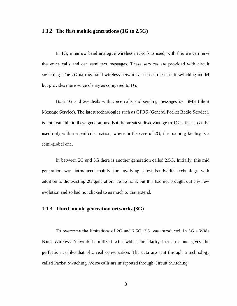
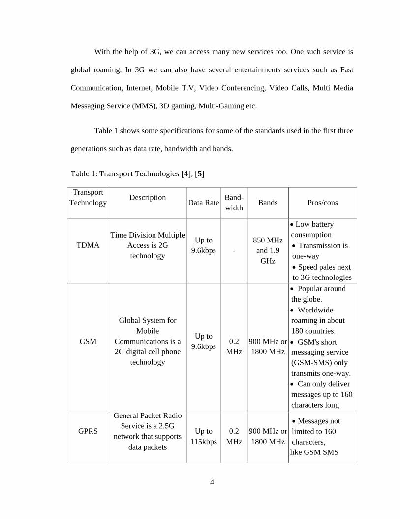
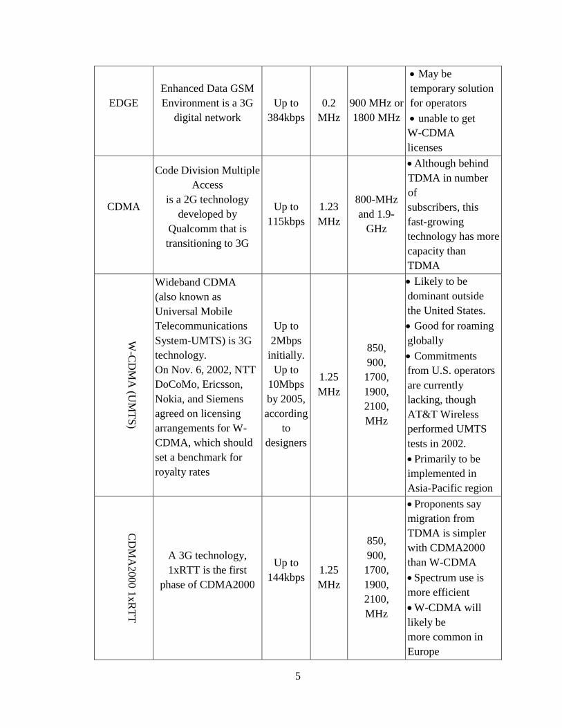
Table 1 shows some specifications for some of the standards used in the first three
generations such as data rate, bandwidth and bands.
Table 1: Transport Technologies [4], [5]
Transport
Technology
Description
Data Rate
Band-
width Bands Pros/cons
TDMA
Time Division Multiple
Access is 2G
technology
Up to
9.6kbps
-
850 MHz
and 1.9
GHz
Low battery
consumption
Transmission is
one-way
Speed pales next
to 3G technologies
GSM
Global System for
Mobile
Communications is a
2G digital cell phone
technology
Up to
9.6kbps
0.2
MHz
900 MHz or
1800 MHz
Popular around
the globe.
Worldwide
roaming in about
180 countries.
GSM's short
messaging service
(GSM-SMS) only
transmits one-way.
Can only deliver
messages up to 160
characters long
GPRS
General Packet Radio
Service is a 2.5G
network that supports
data packets
Up to
115kbps
0.2
MHz
900 MHz or
1800 MHz
Messages not
limited to 160
characters,
like GSM SMS
5
EDGE
Enhanced Data GSM
Environment is a 3G
digital network
Up to
384kbps
0.2
MHz
900 MHz or
1800 MHz
May be
temporary solution
for operators
unable to get
W-CDMA
licenses
CDMA
Code Division Multiple
Access
is a 2G technology
developed by
Qualcomm that is
transitioning to 3G
Up to
115kbps
1.23
MHz
800-MHz
and 1.9-
GHz
Although behind
TDMA in number
of
subscribers, this
fast-growing
technology has more
capacity than
TDMA
W-C
DM
A (U
MT
S)
Wideband CDMA
(also known as
Universal Mobile
Telecommunications
System-UMTS) is 3G
technology.
On Nov. 6, 2002, NTT
DoCoMo, Ericsson,
Nokia, and Siemens
agreed on licensing
arrangements for W-
CDMA, which should
set a benchmark for
royalty rates
Up to
2Mbps
initially.
Up to
10Mbps
by 2005,
according
to
designers
1.25
MHz
850,
900,
1700,
1900,
2100,
MHz
Likely to be
dominant outside
the United States.
Good for roaming
globally
Commitments
from U.S. operators
are currently
lacking, though
AT&T Wireless
performed UMTS
tests in 2002.
Primarily to be
implemented in
Asia-Pacific region
CD
MA
2000 1
xR
TT
A 3G technology,
1xRTT is the first
phase of CDMA2000
Up to
144kbps
1.25
MHz
850,
900,
1700,
1900,
2100,
MHz
Proponents say
migration from
TDMA is simpler
with CDMA2000
than W-CDMA
Spectrum use is
more efficient
W-CDMA will
likely be
more common in
Europe
6
CDMA
2000
1xEV-DO
Delivers data on a
separate channel
Up to
2.4Mbps
1.25
MHz
850,
900,
1700,
1900,
2100,
MHz
(see CDMA2000
1xRTT above)
CDMA
2000
1xEV-DV
Integrates voice and
data on the same
channel
Up to
2.4Mbps
1.25,
3.75
MHz
(see CDMA2000
1xRTT above)
1.1.4 Future mobile generation networks (4G)
The objective of 3G was to develop a new protocol and new technologies to
further enhance the mobile experience. In contrast, the new 4G framework to be
established will try to accomplish new levels of user experience and multi-service
capacity by also integrating all the mobile technologies that exist (e.g. GSM - Global
System for Mobile Communications, GPRS, IMT-2000 - International Mobile
Communications, Wi-Fi, and Bluetooth). [6]
In addition to the services of 3G, 4 G will have some additional features such as
Multi-Media Newspapers and T.V programs with the clarity as to that of an ordinary T.V.
In addition, we can send Data much faster than that of the previous generations. Due to
some key enabling technologies 4G systems are given the standard name Long Term
Evolution (LTE)
7
1.2 Long Term Evolution (LTE)
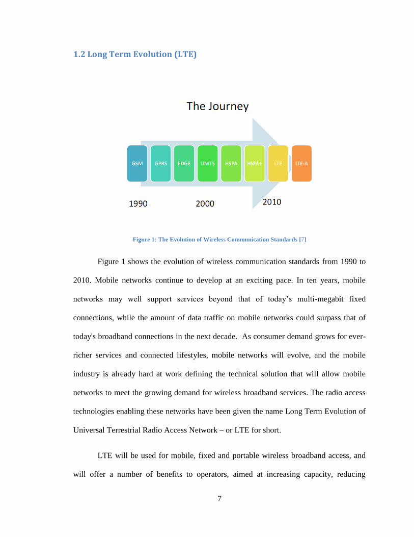
Figure 1: The Evolution of Wireless Communication Standards [7]
Figure 1 shows the evolution of wireless communication standards from 1990 to
2010. Mobile networks continue to develop at an exciting pace. In ten years, mobile
networks may well support services beyond that of today’s multi-megabit fixed
connections, while the amount of data traffic on mobile networks could surpass that of
today's broadband connections in the next decade. As consumer demand grows for ever-
richer services and connected lifestyles, mobile networks will evolve, and the mobile
industry is already hard at work defining the technical solution that will allow mobile
networks to meet the growing demand for wireless broadband services. The radio access
technologies enabling these networks have been given the name Long Term Evolution of
Universal Terrestrial Radio Access Network – or LTE for short.
LTE will be used for mobile, fixed and portable wireless broadband access, and
will offer a number of benefits to operators, aimed at increasing capacity, reducing

8
network complexity and thus lowering deployment and operational costs. It will enable
operators to meet the growing demand for mobile data solutions, making it possible for
richer services to be delivered to consumers more cost effectively. [8]
1.2.1 What is LTE?
LTE (Long Term Evolution) is the trademarked project name of a high
performance air interface for cellular mobile telephony. It is a project of the 3rd
Generation Partnership Project (3GPP), operating under a named trademarked by one of
the associations within the partnership, the European Telecommunications Standards
Institute
The recent increase of mobile data usage and emergence of new applications such
as mobile TV, MMOG (Multimedia Online Gaming) and streaming contents have
motivated the use of (LTE) standards. LTE is the latest in the mobile network technology
that ensures competitive edge over its existing standards: GSM/EDGE and
UMTS/HSxPA [9], where HSPA means High Speed Packet Access is a collection of two
mobile telephony protocols, High Speed Downlink Packet Access (HSDPA) and High
Speed Uplink Packet Access (HSUPA), that extends and improves the performance of
existing WCDMA protocols.
LTE, whose radio access is called "Evolved UMTS Terrestrial Radio Access
Network (E-UTRAN)", is expected to substantially improve end-user throughputs, sector
capacity and reduce user plane latency, bringing significantly improved user experience
9
with full mobility. With the emergence of Internet Protocol (IP) for carrying all types of
traffic, LTE is scheduled to provide support for IP-based traffic with end-to-end Quality
of service (QoS). Voice traffic will be supported mainly as Voice over IP (VoIP)
enabling better integration with other multimedia services. Initial deployments of LTE
are expected by 2010 and commercial availability on a larger scale are expected 1-2 years
later [9].
LTE uses Evolved Packet Core (EPC) network architecture to support the E-
UTRAN which reduces the number of network elements, simplifies functionality,
improves redundancy, but most importantly allows for connections and hand-over to
other fixed line and wireless access technologies in a flawless manner. The aggressive
performance of LTE rely on physical layer technologies, such as, Orthogonal Frequency
Division Multiplexing (OFDM), Multiple-Input Multiple-Output (MIMO) systems and
Smart Antennas to achieve these targets. The main objective of LTE is to minimize the
system and user-equipment complexities for high data throughput and reduced latency.
1.2.2 LTE Bands
There are a large number of allocations or radio spectrum that has been reserved
for FDD (Frequency Division Duplex) LTE use. Table 2 shows the 14 E-UTRAN band
used by the LTE standard for each downlink and uplink for both UE (User Equipment)
and eNB (evolved NodeB) with the minimum and maximum frequencies for downlink
and uplink for every band. Also it shows more than 18000 channels divided to these
bands.
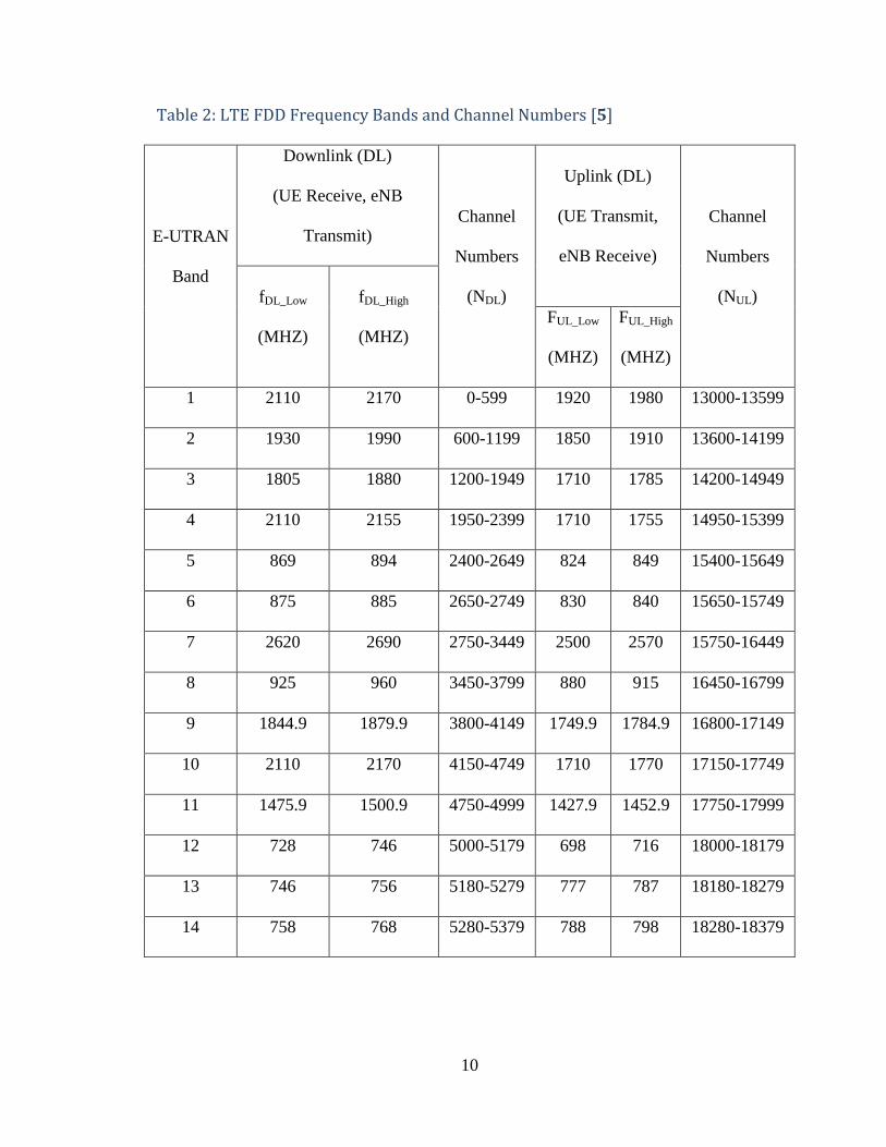
10
Table 2: LTE FDD Frequency Bands and Channel Numbers [5]
E-UTRAN
Band
Downlink (DL)
(UE Receive, eNB
Transmit) Channel
Numbers
(NDL)
Uplink (DL)
(UE Transmit,
eNB Receive)
Channel
Numbers
(NUL) fDL_Low
(MHZ)
fDL_High
(MHZ) FUL_Low
(MHZ)
FUL_High
(MHZ)
1 2110 2170 0-599 1920 1980 13000-13599
2 1930 1990 600-1199 1850 1910 13600-14199
3 1805 1880 1200-1949 1710 1785 14200-14949
4 2110 2155 1950-2399 1710 1755 14950-15399
5 869 894 2400-2649 824 849 15400-15649
6 875 885 2650-2749 830 840 15650-15749
7 2620 2690 2750-3449 2500 2570 15750-16449
8 925 960 3450-3799 880 915 16450-16799
9 1844.9 1879.9 3800-4149 1749.9 1784.9 16800-17149
10 2110 2170 4150-4749 1710 1770 17150-17749
11 1475.9 1500.9 4750-4999 1427.9 1452.9 17750-17999
12 728 746 5000-5179 698 716 18000-18179
13 746 756 5180-5279 777 787 18180-18279
14 758 768 5280-5379 788 798 18280-18379
11
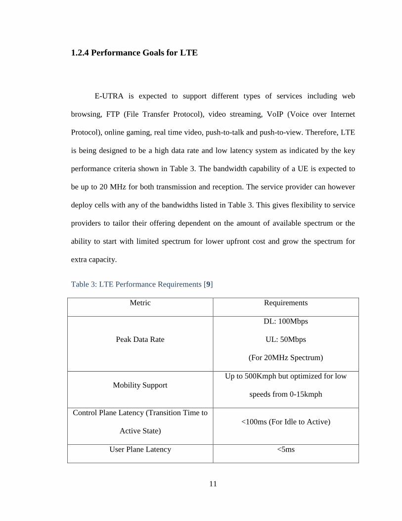
1.2.4 Performance Goals for LTE
E-UTRA is expected to support different types of services including web
browsing, FTP (File Transfer Protocol), video streaming, VoIP (Voice over Internet
Protocol), online gaming, real time video, push-to-talk and push-to-view. Therefore, LTE
is being designed to be a high data rate and low latency system as indicated by the key
performance criteria shown in Table 3. The bandwidth capability of a UE is expected to
be up to 20 MHz for both transmission and reception. The service provider can however
deploy cells with any of the bandwidths listed in Table 3. This gives flexibility to service
providers to tailor their offering dependent on the amount of available spectrum or the
ability to start with limited spectrum for lower upfront cost and grow the spectrum for
extra capacity.
Table 3: LTE Performance Requirements [9]
Metric Requirements
Peak Data Rate
DL: 100Mbps
UL: 50Mbps
(For 20MHz Spectrum)
Mobility Support
Up to 500Kmph but optimized for low
speeds from 0-15kmph
Control Plane Latency (Transition Time to
Active State)
<100ms (For Idle to Active)
User Plane Latency <5ms
12
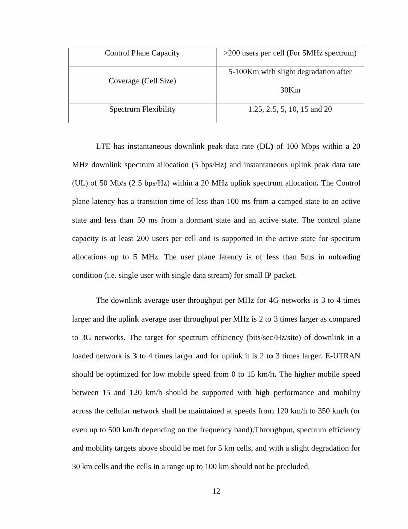
Control Plane Capacity >200 users per cell (For 5MHz spectrum)
Coverage (Cell Size)
5-100Km with slight degradation after
30Km
Spectrum Flexibility 1.25, 2.5, 5, 10, 15 and 20
LTE has instantaneous downlink peak data rate (DL) of 100 Mbps within a 20
MHz downlink spectrum allocation (5 bps/Hz) and instantaneous uplink peak data rate
(UL) of 50 Mb/s (2.5 bps/Hz) within a 20 MHz uplink spectrum allocation. The Control
plane latency has a transition time of less than 100 ms from a camped state to an active
state and less than 50 ms from a dormant state and an active state. The control plane
capacity is at least 200 users per cell and is supported in the active state for spectrum
allocations up to 5 MHz. The user plane latency is of less than 5ms in unloading
condition (i.e. single user with single data stream) for small IP packet.
The downlink average user throughput per MHz for 4G networks is 3 to 4 times
larger and the uplink average user throughput per MHz is 2 to 3 times larger as compared
to 3G networks. The target for spectrum efficiency (bits/sec/Hz/site) of downlink in a
loaded network is 3 to 4 times larger and for uplink it is 2 to 3 times larger. E-UTRAN
should be optimized for low mobile speed from 0 to 15 km/h. The higher mobile speed
between 15 and 120 km/h should be supported with high performance and mobility
across the cellular network shall be maintained at speeds from 120 km/h to 350 km/h (or
even up to 500 km/h depending on the frequency band).Throughput, spectrum efficiency
and mobility targets above should be met for 5 km cells, and with a slight degradation for
30 km cells and the cells in a range up to 100 km should not be precluded.
13
Co-existence in the same geographical area and co-location with
GERAN/UTRAN on adjacent channels is also accounted for. GERAN is an abbreviation
for GSMEDGE Radio Access Network. The standards for GERAN are maintained by the
3GPP (Third Generation Partnership Project). GERAN is a key part of GSM, and also of
combined UMTS/GSM networks. GERAN is the radio part of GSM/EDGE together with
the network that joins the base stations and the base station controllers. The network
represents the core of a GSM network, through which phone calls and packet data are
routed from and to the PSTN and Internet to and from subscriber handsets. A mobile
phone operator's network comprises one or more GERANs, coupled with UTRANs in the
case of a UMTS/GSM network.
A GERAN network without EDGE is a GRAN, but is otherwise identical in concept.
A GERAN network without GSM is an ERAN
1.2.5 Enabling Technologies in LTE
A) MIMO
The Shannon-Hartley capacity theorem predicts that the capacity of the error free
channel for a single-input-single-output (SISO) system is given by:
SNRBC 1log2 (1.1)
where, C is the capacity in bits/second, B is the channel bandwidth and SNR is the linear
signal-to-noise ratio value. In a MIMO system, the cross-coupling between the signals
14
from the transmit antennas to the receive antennas introduces a path dependency through
the radio channel. This will impact the overall capacity of the system as [10]:
SNRk
BCR
I 2log (1.2)
where, C is the channel capacity in bit/second, I is the identity matrix, R is the channel
and antenna correlation matrix, k is rank of R (i.e. number of transmit antennas).
Equation (1.2) can also be written as
2log 1 * * (1.3)T RC B M N SNR
where, MT is the number of transmit antennas, NR is the number of receive antennas.
For diversity and MIMO applications, the correlation between signals received by
the involved antennas at the same side of a wireless link is an important figure of merit of
the whole system. Usually, the envelope correlation is presented to evaluate the diversity
capabilities of a multi-antenna system [11]. It can be measured directly in a representative
scattering environment, or calculated from the full-sphere radiation patterns. Both
methods require special measurement equipment and are time-consuming. [12]
For isotropic signal environments the received signal correlation can be found
from a simpler and faster method than the one previously described. The method derives
the correlation coefficient from the S-parameters of the antennas, i.e., the port reflection
coefficients S11 and S22 of the two antennas, and the coupling S21=S12. Several
publications present the relation between the S-parameters and the correlation coefficient
15
[13] [14] [15]. What are missing in these relations are the radiation efficiencies of the two
antennas.
This parameter (Correlation Coefficient) should be preferably computed from 3D
radiation patterns but this method requires a lot of work [13] and may suffer from errors
if no sufficient pattern cuts are taken into account in the computation.
The Total radiated powers for the two antennas can be expressed as;
2 2
1 11 21 1
2 2
2 22 12 2
1 (1.4)
1 (1.5)
rad
rad
P S S
P S S
from which the definition of radiation efficiencies 1 and 2 are clear, and the internal
losses for the two antennas are given by
2 2
1 11 21 1
2 2
2 22 12 2
1 1 (1.6)
1 1 (1.7)
loss
loss
P S S
P S S
The relation for the correlation coefficient is derived on the basis of orthogonality
between two signals of separate independent sources. This is the fundamental principle
and is described in most microwave books as a requirement of zero correlation between
two columns in an S-matrix [16]. Generalized S-parameters should be used when ports
have different impedances [17], which means that S-parameters are adjusted so that each
signal’s amplitude is proportional to the square root of the corresponding power. The
requirement of zero correlation is valid for lossless S-matrices, but internal losses are
easily incorporated by treating the losses as additional ports where power is terminated.
16
Generally, the S-matrix is an applicable tool to model the signal flow of any
device. To derive a general relation for orthogonality, assume that the amplitudes of the
complex signals from two sources are denoted by E1 and E2, respectively, both being
functions over volume. These functions E1 and E2 are vectors of S-parameters according
to eq. 1.8
1 Nk ... S (1.8)T
k kE S
where N is the number of ports. The impedance function Z is also introduced for the
purpose of making E1 and E2 correspond to generalize S-parameters. The orthogonality
between the signals is then simply
*
1 2
Ptot
E1(1,2) (1.9)
tot
Eort dP
P Z
where Ptot is the total power. The amplitudes E1 and E2 should be normalized so that
dividing by Ptot results in an orthogonality with a magnitude between zero and unity.
Using the analogy in (1.8) in conjunction with the requirement of orthogonality between
two columns of the S-matrix renders the conclusion that ort(1,2) should be zero.
Now consider a pair of antennas, and let E1 and E2 be the signals scattered at the
ports and over the sphere. The total S-matrix can be divided into one S-matrix for the
antenna ports and one for the radiation functions, after which orthogonality is applied to
the sum of the two [13]. A third S-matrix is introduced to account for the losses, and
orthogonality then applies to the sum of all three. With the antennas described by their S-
parameters and relative powers according to (1.4)–(1.7), the requirement for
orthogonality takes the form
17
* *
11 12 21 22 rec rad1 rad2 loss loss1 loss2S S +S S + P P + P P =0 (1.10)
where rec and loss are the normalized complex correlation coefficients of the radiation
patterns and the internal losses, respectively. Multiplying by the square root of the
powers in the two last terms in (1.10) is done for the purpose of making the terms
correspond to generalize S-parameters. The first two terms also need such normalization,
but because all powers (Prad and Ploss) are relative to these powers, they are in effect unity.
Substituting (1.4)–(1.7) into (1.10) gives the expression relating correlation
coefficients to S-parameters and radiation efficiencies
* *
11 12 21 22rec 1 2 loss 1 2
2 2 2 2
11 21 22 12
S S +S S+ + (1- )(1- )=0 (1.11)
1 1S S S S
Since the expression on the left-hand side in (1.11) is zero, one unknown term can
be calculated if the other terms are known. The principle of calculating received signal
correlation from S-parameters is to measure the first term and take the second term to be
the negative of this value. The last term in (1.11) is then omitted or assumed to be zero.
Assuming that the antennas will operate in a uniform multi-path environment, an
alternative consists in computing this parameter from its scattering parameters definition
[13]. The envelope correlation of two antennas is given by Eq. 1.12
* *
11 12 21 2212 max 2 2 2 2
1 211 21 22 12 1 2
1 11 1
1 1
S S S S
S S S S
(1.12)
18
Where,12 max : is the upper bound of the signal correlation coefficient between antenna 1
and antenna 2, S11is is the reflection coefficient of the antenna number 1, S22 is the
reflection coefficient of the antenna number 2, S21, S12: are the transmission parameters
between the two antennas, *
.
means the conjugate complex value, 1 2, are the
radiation efficiencies of antennas 1 and 2, respectively.
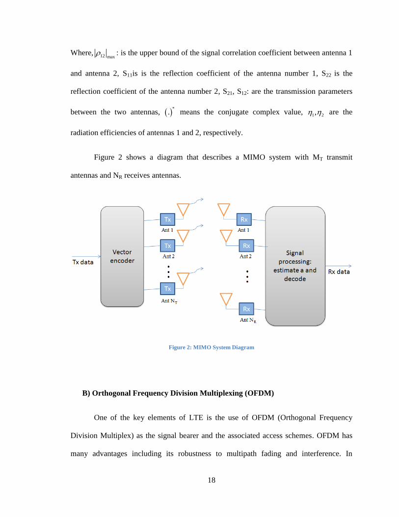
Figure 2 shows a diagram that describes a MIMO system with MT transmit
antennas and NR receives antennas.
Figure 2: MIMO System Diagram
B) Orthogonal Frequency Division Multiplexing (OFDM)
One of the key elements of LTE is the use of OFDM (Orthogonal Frequency
Division Multiplex) as the signal bearer and the associated access schemes. OFDM has
many advantages including its robustness to multipath fading and interference. In
19
addition to this, even though, it may appear to be a particularly complicated form of
modulation, it lends itself to digital signal processing techniques.
One of the key parameters associated with the use of OFDM within LTE is the
choice of bandwidth. The available bandwidth influences a variety of decisions including
the number of carriers that can be accommodated in the OFDM signal and in turn this
influences elements including the symbol length and so forth.
LTE defines a number of channel bandwidths. Obviously the greater the
bandwidth, the greater the channel capacity.
1.2.6 LTE Antennas
Small and conformal antennas are fundamental to the development of mobile
communication devices. Printed antennas are always used in mobile terminals, but for
780 MHz it will be a challenge using conventional ways. Recently, meander line
technology is adopted to design small but wideband antennas, were size of the radiating
element at a given frequency is reduced by a factor that is proportional to the number of
turns. Due to the small size of printed meander line antenna (MLA), they are directly
embedded within the mobile handsets. In addition, they feature an improvement in
efficiency, resulting in longer battery life than other handsets currently available on the
market today. Furthermore, MLA technology allows engineers to design ultra-broadband
antennas capable of operating at multiple frequencies and in a variety of modes.
20
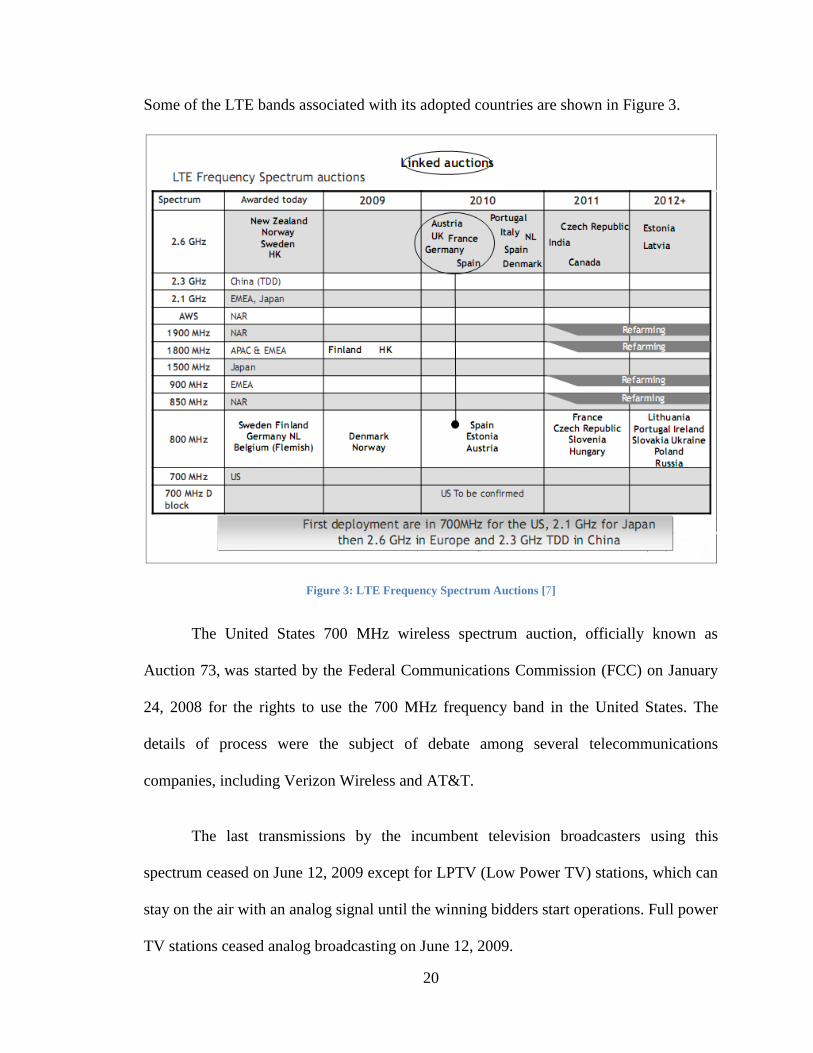
Some of the LTE bands associated with its adopted countries are shown in Figure 3.
Figure 3: LTE Frequency Spectrum Auctions [7]
The United States 700 MHz wireless spectrum auction, officially known as
Auction 73, was started by the Federal Communications Commission (FCC) on January
24, 2008 for the rights to use the 700 MHz frequency band in the United States. The
details of process were the subject of debate among several telecommunications
companies, including Verizon Wireless and AT&T.
The last transmissions by the incumbent television broadcasters using this
spectrum ceased on June 12, 2009 except for LPTV (Low Power TV) stations, which can
stay on the air with an analog signal until the winning bidders start operations. Full power
TV stations ceased analog broadcasting on June 12, 2009.
21
The 700 MHz spectrum was previously used for analog television broadcasting.
The FCC has ruled that the switch to digital television has made these frequencies no
longer necessary for broadcasters, due to the improved spectral efficiency of digital
broadcasts. Thus, all broadcasters will be required to move to newer channels as part of
the digital TV transition. Some of the 700 MHz spectrum was already in some areas are
already being used for broadcasting and Internet access. For example Qualcomm
MediaFLO in 2007 started using Channel 55 for broadcasting TV to cell phones in New
York City, San Diego and elsewhere. [18]
1.3 Thesis Motivation
In the recent years, there has been rapid growth in wireless communication. With
the increasing number of users and limited bandwidth available, operators are trying hard
to optimize the network for larger capacity and improved quality coverage. This has led
to the field of antenna engineering to constantly evolve and accommodate the need for
wideband, low-cost, miniaturized and easily integrated antennas [19].
Since LTE will be the technology used for the next generation of mobile
communication which will be implemented by the end of this year and will be
commercialized by the coming years, there will be a huge demand for it. Because of these
reasons, mobile phones should be compatible with the technology mentioned above and
in order to achieve this, mobile antennas should be properly designed according to the
new LTE standards.
22
In this thesis, we propose a 2 element MIMO antenna system operating in 700
MHz band which is one of the newest and the most challenging bands for designing an
antenna within the LTE specifications.
1.4 Thesis Objectives
The objectives for this work are the following:
1. Design and optimize a single element and a 2-element (MIMO) meander line antenna
system for LTE standards. The design should fit within a cellular phone handset size and
satisfy the following requirements.
(a) Operating frequency of 780 MHz with a bandwidth greater than 40 MHz
(b) Isolation between the two elements MIMO antenna should be less than -15 dB
(c) Size of the 2-element MIMO antenna should fit with an area of 40x50 mm2
2. To study the correlation coefficient for the 2-element MIMO antenna for this band and
come up with a novel technique to reduce it to a value less than 0.3
4. Fabricate a single and 2-element Meander line antenna and experimentally observe
their characteristics using a ―network analyzer‖ and the ―Antenna Test and Measurement
System‖.
5. Compare and comment on the simulated and experimentally obtained reflection and
radiation responses of the single and 2 element MIMO antennas.
23
1.5 Thesis Overview
The thesis is organized in six chapters as follows:
Chapter 2 of this thesis starts with an introduction of the types of mobile printed
antennas and electrically small antennas and it summarizes the reviewed literature. In
Chapter 3, the design of electrically small antenna (ESA) is described, where the first part
describes the designing of a Meander Line Antenna (MLA), second part is dedicated to
introduce PIFA antenna and to compare between these two designs, the simulation results
of the two proposed antennas will be discussed as well. Chapter 4 discusses all the design
of a dual element MIMO antenna system using ESA then study the correlation coefficient
that will arise from this system then modify the design to reduce its effect. The simulated
(HFSS) radiation characteristics associated with the designed antenna will be discussed in
this chapter also. In Chapter 5, the experimentally observed results for single antenna and
2-element MIMO antenna are then presented and analyzed. Comparisons between the
experimental and simulated results for both single and dual element MIMO antenna are
also tabulated in this chapter. Finally chapter 6 describes the conclusions drawn from this
research work and recommendations on future work to be carried on this subject.
24
CHAPTER 2
LITERATURE REVIEW
2.1 Introduction
The development of small integrated printed antennas plays a significant role in
the progress of rapidly expanding wireless communication applications. They are
increasingly used in wireless communication systems due to advantages of being
lightweight, compact and conformal. Recent evolution of mobile phones and
RF/microwave networks demanded miniaturized version of printed antennas, which often
employs: (i) High permittivity substrate. (ii) Shorting pins. (iii) Meandering or
combination of these and other approaches. [20]
In mobile communication, Meander line antennas are recently favored over other
printed antennas due to its simplicity and ease in integration. The following sections
briefly discuss the evolution and characteristics of Meander line antennas (MLA).
The design process of 1.025 GHz meander line antenna, described in the literature
[21], a design a meander line antenna operating at 1025MHz using empirical equations is
discussed that give a certain dimensions for the width, length, number of turns and
25
spacing at a certain frequency, and then they test their design to check the validity of
these equations. The value so obtained by two methods one by empirical relation and
other by design equation are compared. It is found that the dimension obtained by both
methods matched. Thus one can use these empirical relations for designing the meander
line antenna, but the problem of this design that the dimensions of this antenna is too big
(as will be shown in results section) but it give us an idea how the meander works and
how it resonate at that frequency.
A more compact design of a meander line antenna, available in the literature [22],
was designed to operate at 2.4-GHz for WLAN application. The paper described two
different designs of meander line antenna with and without conductor line. The designed
antennas were fabricated on a double-sided FR-4 printed circuit board using standard
PCB technique and tested with a Network Analyzer. A bandwidth of 152MHz and return
loss of -37.7dB were obtained at the operating center frequency of 2.4GHz. The effect on
the antenna radiation and reflection properties with varying the MLA length, width,
number of turns and conductor dimensions are also discussed in this paper.
In reference [23], a meander line antenna with smaller dimensions (40 by 40 cm)
are presented. The designed antenna exhibited a bandwidth of 274 MHz and return loss
of -25 dB at a center frequency of 1.575 GHz. This design is of importance to this
research work due to the similarity of the antenna dimensions and will be carefully
investigated.
Reference [24], discusses the design process of two electrically small printed
antennas, suitable for mobile communication handsets. In this design, the resonant
frequency of the antenna is significantly reduced by employing shorted patches, which
26
maximizes the length of the current path for a given area. In the literature, reductions in
operating frequencies are also achieved using different methods, such as; shorting posts
[25], high dielectric constant material [26], resistive loads [27], and deformation of the
conductor shape (in addition to using a shorting post) [28], each with their relative merits
and disadvantages.
It is evident from the literature review that most of the designed antenna with
reduced element size have the trend to use higher frequency bands (i.e. 2.4 GHz and 5.5
GHz) [25], [27]- [29]. But little references are available for designing low frequency
antennas with limited size. This is particularly important for the most recent initiative to
adopt the 700 MHz band for 4th generation (LTE) of cellular phones by AT&T, Verizon
and other world leaders in wireless technologies. In this research work, a 700 MHz
antenna with limited dimensions will be designed for LTE applications. Although similar
antenna is available in the literature [30], but needs to be improved in terms of antenna
efficiency and cost-effectiveness.
Reference [31] describes the design process of a PIFA antenna with two separate
patches of different sizes for operating in two different bands. The larger and smaller
patches have separate shorting points and are operated, respectively, in the 900 and 1800
MHz bands as quarter-wavelength resonant structures. A dual feed (feed point 1 for the
larger patch and feed point 2 for the smaller patch) is also utilized in the design, which
can find application where mobile phones have receivers with dual front ends. In
addition, to achieve a compact antenna size, a portion of the larger patch is removed to
accommodate the smaller patch. A compact 900/1800 MHz dual-frequency PIFA with an
area of 25x26 mm2 and a height of 4 mm has been presented in [32], This design has a
27
capacitive load, fed by a capacitive feed and uses a substrate with a relative permittivity
of 2.1 between the two top patches and the ground plane.
Instead of using a simple flat ground plane, a PIFA with an L-shaped ground
plane has also been studied in literature. It has been found that such a PIFA can have
decreased backward radiation and enhanced antenna gain. A related study is reported in
Reference [33]. An additional vertical ground is added to the edge of the horizontal
ground plane in the proposed design to enhance the antenna performance. This shape will
be thoroughly studied in this research work to fabricate a similar 700 MHz PIFA antenna.
The radiation and reflection performances of the PIFA and meander-line antenna will
then be compared.
2.2 Printed Antenna for Mobile Devices
Planner antennas are low profile, cost-effective and flat in appearance which
makes them suitable for recent communication systems, such as the Global System for
Mobile (GSM; 890-960 MHz), the Digital Communication System (DCS; 1710-1880
MHz), the Personal Communication System (PCS; 1850-1990 MHz), the Universal
Mobile Telecommunication System (UMTS; 1920-2170), the Wireless Local Area
Networks (WLANs) in the 2.4 GHz (2400-2484 MHz) and 5.2 GHz (5150-5350 MHz)
bands [30] and Long Term Evolution (LTE) in the 700 MHz (758-798 MHz). LTE is a
new standard for wireless communication that FCC has recently agreed to adopt for the
4th
generation cellular phones. Before LTE antennas can be designed with confidence,
basic characteristics of antennas in general needs to be understood.
28
2.2.1 Antenna Basics
According to the IEEE Standard Definitions, the antenna or aerial is defined as ―a
means of radiating or receiving radio waves" [19]. In other words, antennas act as an
interface for electromagnetic energy, propagating between free space and guided
medium. Amongst the various types of antennas that include wire antennas, aperture
antennas, reflector antennas, lens antennas etc., microstrip patches are one of the most
versatile, conformal and easy to fabricate antennas.
Good antenna design is a critical factor in obtaining good range and stable
throughput in a wireless application. This is especially true in low power and compact
designs where antenna space is less than optimal. To obtain the desired performance, it is
required that users have at least a basic knowledge about how antennas function and the
design parameters involved. These parameters include selecting the correct antenna,
antenna tuning, matching, gain/loss, and knowing the required radiation pattern.
2.2.1.1 Basic Antenna Parameters: Some of the basic antenna characteristics that a
designer should be familiar with before starting the design process are briefly described
below:
Antenna gain
Relates the intensity of an antenna in a given direction to the intensity that would
be produced by a hypothetical ideal antenna that radiates equally in all directions
(isotropically) and has no losses.
29
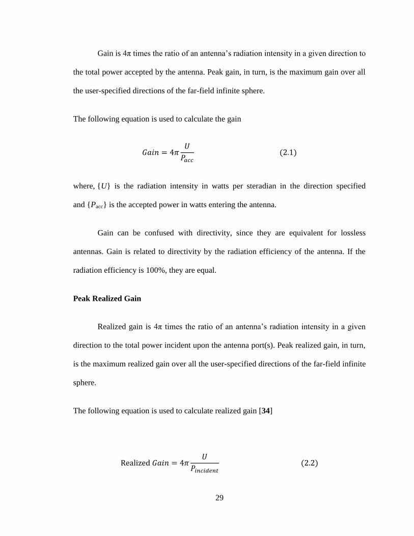
Gain is 4π times the ratio of an antenna’s radiation intensity in a given direction to
the total power accepted by the antenna. Peak gain, in turn, is the maximum gain over all
the user-specified directions of the far-field infinite sphere.
The following equation is used to calculate the gain
where, U is the radiation intensity in watts per steradian in the direction specified
and Pacc is the accepted power in watts entering the antenna.
Gain can be confused with directivity, since they are equivalent for lossless
antennas. Gain is related to directivity by the radiation efficiency of the antenna. If the
radiation efficiency is 100%, they are equal.
Peak Realized Gain
Realized gain is 4π times the ratio of an antenna’s radiation intensity in a given
direction to the total power incident upon the antenna port(s). Peak realized gain, in turn,
is the maximum realized gain over all the user-specified directions of the far-field infinite
sphere.
The following equation is used to calculate realized gain [34]
30
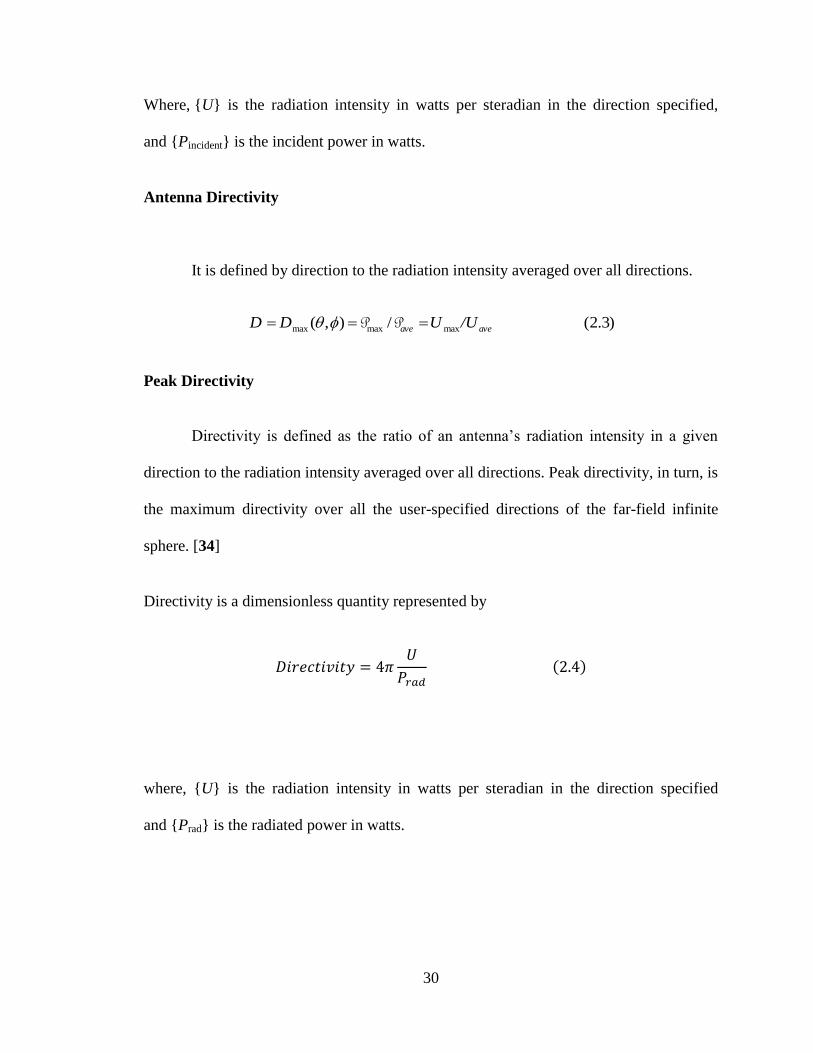
Where, U is the radiation intensity in watts per steradian in the direction specified,
and Pincident is the incident power in watts.
Antenna Directivity
It is defined by direction to the radiation intensity averaged over all directions.
Peak Directivity
Directivity is defined as the ratio of an antenna’s radiation intensity in a given
direction to the radiation intensity averaged over all directions. Peak directivity, in turn, is
the maximum directivity over all the user-specified directions of the far-field infinite
sphere. [34]
Directivity is a dimensionless quantity represented by
where, U is the radiation intensity in watts per steradian in the direction specified
and Prad is the radiated power in watts.
max max max( , ) / (2.3)ave aveD D U /U P P

31
• For a lossless antenna, the directivity will be equal to the gain. However, if the antenna
has inherent losses, the directivity is related to the gain by the radiation efficiency of the
antenna.
Antenna Bandwidth
It is defined as the range of frequencies within which the performance of the
antenna, with respect to some characteristics, conforms to a specified standard [19].
Antenna Radiation Patterns
An antenna radiation pattern is a 3-D plot of its radiation far from the source.
Antenna radiation patterns usually take two forms, the elevation pattern and the azimuth
pattern. The elevation pattern is a graph of the energy radiated from the antenna looking
at it from the side (E-Plane). The azimuth pattern is a graph of the energy radiated from
the antenna as if you were looking at it from directly above the antenna (H-Plane).
Maximum intensity (Max U)
The radiation intensity U is the power radiated from an antenna per unit solid
angle. The maximum intensity of the radiation is measured in watts per steradian and is
calculated by [34]
| |

32
where, U (,) is the radiation intensity in watts per steradian, |E| is the magnitude of
the E-field, 0 is the intrinsic impedance of free space and it is equal to 376.7
ohms, r is the distance from the antenna, in meters.
Radiated Power
Radiated power is the amount of time-averaged power (in watts) exiting a
radiating antenna structure through a radiation boundary.
For a general radiating structure, radiated power is computed as [34]
∫
where, Prad is the radiated power in watts; Re is the real part of a complex
number, s represents the radiation boundary surfaces, E is the radiated electric
field, H* is the conjugate of H and ds is the local radiation-boundary unit normal
directed out of the 3D model.
Accepted Power
The accepted power is the amount of time-averaged power (in watts) entering a
radiating antenna structure through one or more ports. For antennas with a single port,
accepted power is a measure of the incident power reduced by the mismatch loss at the
port plane. [34]
For a general radiating structure, accepted power is computed as
33
∫
where, Pacc is the accepted power in watts, Re is the real part of a complex number,
A is the union of all port boundaries in the model, E is the radiated electric
field, H* is the conjugate of H and ds is the local port-boundary unit normal directed
into the model.
For the simple case of an antenna with one lossless port containing a single
propagating mode, the above expression reduces to [34]
| | | |
where, a is the complex modal excitation specified, s11 is the reflection coefficient of
the antenna.
Incident Power
Incident power is the total amount of time-averaged power (in watts) incident
upon all port boundaries of an antenna structure.
For the simple case of an antenna with one lossless port containing a single
propagating mode, the incident power Pincident is given by [34]
| |
where, a is the complex modal excitation specified.
34
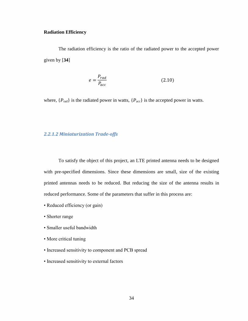
Radiation Efficiency
The radiation efficiency is the ratio of the radiated power to the accepted power
given by [34]
where, Prad is the radiated power in watts, Pacc is the accepted power in watts.
2.2.1.2 Miniaturization Trade-offs
To satisfy the object of this project, an LTE printed antenna needs to be designed
with pre-specified dimensions. Since these dimensions are small, size of the existing
printed antennas needs to be reduced. But reducing the size of the antenna results in
reduced performance. Some of the parameters that suffer in this process are:
• Reduced efficiency (or gain)
• Shorter range
• Smaller useful bandwidth
• More critical tuning
• Increased sensitivity to component and PCB spread
• Increased sensitivity to external factors
35
Several performance factors deteriorate with miniaturization, but some antenna
types tolerate miniaturization better than others. How much a given antenna can be
reduced in size depends on the actual requirements for range, bandwidth, and
repeatability. In general, an antenna can be reduced to half its natural size with moderate
impact on performance. However, after a 1/2 reduction, performance becomes
progressively worse as the radiation resistance drops off rapidly. As loading and antenna
losses often increase with reduced size, it is clear that efficiency drops off quite rapidly
[35].
2.2.2 Printed Antennas
The leading printed antennas commonly used in embedded applications are:
Microstrip Lines/Patch, Planar Inverted 'F' (PIFA), Meander Line (MLA) etc. Microstrip
lines are an extension of the monopole. They can be easily fabricated by etching a copper
strip of the radio circuit board. While very inexpensive to make, its performance is
limited by surrounding electronics on the circuit board. Microstrip monopole is also only
a single-frequency solution. Patch antennas are a good choice for a system that requires a
beam pattern focused in a certain direction. Patches are fabricated out of square or round
copper clad on the top surface of a circuit board. Their radiation beam is normal to the
surface of the board. One antenna type becoming increasingly popular is planar inverted-
F antenna (PIFA). The PIFA antenna literally looks like the letter 'F' lying on its side with
the two shorter sections providing feed and ground points and the 'tail' providing the
36
radiating surface. PIFAs make good embedded antennas in that they exhibit a somewhat
omnidirectional pattern and can be made to radiate in more than one frequency band.
PIFA has a low profile, and it can easily be incorporated into wireless handsets. PIFA
antennas are generally used with a ground plane, which is generally the cellular phone
circuit board ground plane. The Meander Line Antenna (MLA) is a new type of radiating
element, made from a combination of a loop antenna and frequency tuning meander lines.
The electrical length of the MLA is made up mostly by the delay characteristic of the
meander line rather than the length of the radiating structure itself. MLAs can be
designed to exhibit broadband capabilities that allow operation on several frequency
bands. For the base stations classical dipoles are very common. The common dipole has
long been recognized as an efficient radiator when cut to the appropriate frequency
length. It is made from bending the end of an open circuit two-wire transmission line into
a 'T' shape, where the top of the 'T' is the radiating section of the antenna. The length of
the top is lambda, the wavelength of the signal. In some applications also monopole
antennas with /2 or /4 length mounted over ground plane are used. There are also
special antenna constructions for special applications. When you need to flood a wide but
defined area with RF energy, such as for perimeter security systems, tunnels, and
cellular- or 802.11-system interior zones, one approach is to use an RF-leaky feeder cable
to provide controlled radiation.

37
2.2.2.1 Microstrip Patch Antenna
In its simplest form a microstrip antenna consists of a dielectric substrate
sandwiched between two conducting surfaces: the antenna plane and the ground plane.
The simplified microstrip patch antenna is shown in Figure 4.
Figure 4: Basic rectangular microstrip patch antenna construction
Microstrip patch antennas radiate primarily because of the fringing fields between
the patch edge and the ground plane. Since the propagating EM fields lay, both in the
substrate and in free space, a quasi-TEM mode is generated. The length and width of the
patch are given by (a) and (b) respectively. The substrate thickness is given by h.
Microstrip antennas are often feed using; Microstrip Line feed [36], Coaxial feed [37],
Proximity coupled [38] and Aperture coupled [38] techniques, each with their own
advantages and disadvantages [19]. The substrate thickness is given by h.
Along with a number of advantages [39] microstrip antennas also suffer from
some disadvantages [36] [37] like narrow bandwidth, low efficiency, low Gain, spurious

38
radiation and surface wave excitation. While spurious radiation and surface waves can be
eliminated by using the right feed mechanisms and substrate thickness [36], the issues of
major concern are poor bandwidth and low radiation efficiency. Microstrip antennas
inherently suffer from Ohmic losses and dielectric losses making it a high Q device [36].
In order to achieve greater bandwidth and gain we must increase substrate thickness but
this could result in surface waves [37].
2.2.2.2 Meander Line Antenna
Meander Line Antenna is a type of printed antenna that achieves miniaturization
in size by embedding the wire structure on a dielectric substrate. MLA technology was
originally developed by BAE SYSTEMS (a former Lockheed Martin Company) [40], for
the Information and Electronic Warfare Systems (IEWS), which require high
performance antennas for both satellite and terrestrial communications. Recently, this
class of antennas are found to be suitable for application mobile handsets; wireless data
networking for laptops, PC cards and access points. In basic form meander line antenna is
a combination of conventional wire and planer strip line. Benefits include configuration
simplicity, easy integration to a wireless device, inexpensive and potential for low
Specific Absorption Rate (SAR) features. SAR is a measure of the rate at which energy is
absorbed by the body when exposed to a radio frequency (RF) electromagnetic field. It is
defined as the power absorbed per mass of tissue and has units of watts per kilogram.
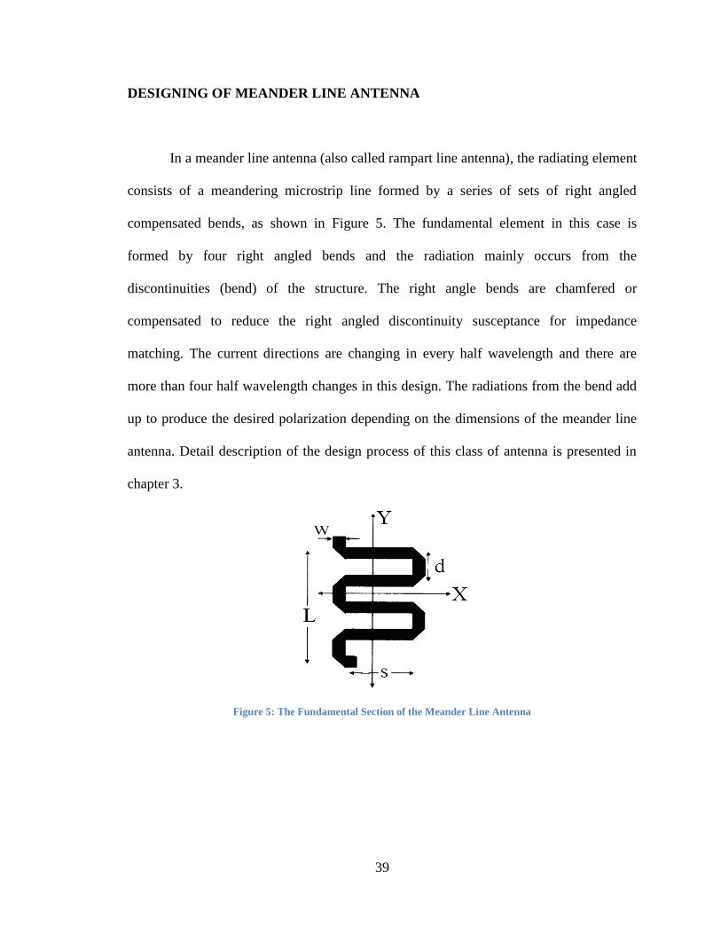
39
DESIGNING OF MEANDER LINE ANTENNA
In a meander line antenna (also called rampart line antenna), the radiating element
consists of a meandering microstrip line formed by a series of sets of right angled
compensated bends, as shown in Figure 5. The fundamental element in this case is
formed by four right angled bends and the radiation mainly occurs from the
discontinuities (bend) of the structure. The right angle bends are chamfered or
compensated to reduce the right angled discontinuity susceptance for impedance
matching. The current directions are changing in every half wavelength and there are
more than four half wavelength changes in this design. The radiations from the bend add
up to produce the desired polarization depending on the dimensions of the meander line
antenna. Detail description of the design process of this class of antenna is presented in
chapter 3.
Figure 5: The Fundamental Section of the Meander Line Antenna
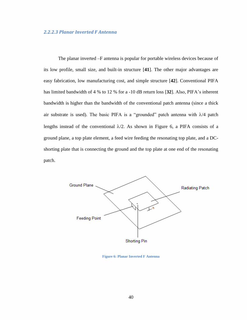
40
2.2.2.3 Planar Inverted F Antenna
The planar inverted –F antenna is popular for portable wireless devices because of
its low profile, small size, and built-in structure [41]. The other major advantages are
easy fabrication, low manufacturing cost, and simple structure [42]. Conventional PIFA
has limited bandwidth of 4 % to 12 % for a -10 dB return loss [32]. Also, PIFA’s inherent
bandwidth is higher than the bandwidth of the conventional patch antenna (since a thick
air substrate is used). The basic PIFA is a ―grounded‖ patch antenna with /4 patch
lengths instead of the conventional /2. As shown in Figure 6, a PIFA consists of a
ground plane, a top plate element, a feed wire feeding the resonating top plate, and a DC-
shorting plate that is connecting the ground and the top plate at one end of the resonating
patch.
Figure 6: Planar Inverted F Antenna
41
PIFA creates an exceptionally uniform 3D signal sphere through its inverted-F
design, which generates an Omni-directional signal field. In comparison to other popular
two-dimensional antenna types, such as IFA (Inverted-F Antenna) and MLA (Meander
Line Antenna), the 3D signal generated by the cubic structure of PIFA-type antennae
offers double the surface area of other antennas guaranteeing the highest levels of
antenna efficiency for enhanced transmission and reception. In this research the antenna
properties of the proposed MLA LTE antenna will be compared with a 2nd
design of
PIFA configuration.
2.3 Electrically Small Antenna
2.3.1 Fundamental Limitations
The fundamental limits on small antenna performance are available in the
literature. In 1947 [43], Wheeler investigated the effects of antenna effective volume on
radiation efficiency and bandwidth. Wheeler described an electrically small antenna as
one with a maximum geometrical dimension much less than the radian length. The radian
length is a distance measurement equal to2
. This is a convenient definition because a
sphere with diameter equal to the radian length contains most of the stored near-field
energy of the electrically small antenna. A year later, Chu derived an approximate lower
limit for the radiation Q of an electrically small antenna [44] Recently, McLean derived
an exact lower limit and corrected apparent errors in the derivation of Q. [45]. In 1987 the
42
monograph Small Antennas by Fujimoto, Henderson, Hirasawa and James summarized
the approaches used to design electrically small antennas (ESA) [46].
Since an ESA is contained within a given volume it has an inherent minimum
value of Q thus there exists a limit on the attainable maximum impedance bandwidth of
an ESA [23]. Note that antennas operating at frequencies outside their normal operating
range of Q-factor (also called Quality Factor) are of little practical utility. Electrically
small and low-profile antennas are both subject to performance limitations due to size
reduction. These classes of antennas have low efficiencies, and are difficult to match to a
transmission line due to low input resistance and high input reactance. In addition, ESAs
typically exhibit narrow impedance bandwidth, which is an important parameter in the
antenna design process.
2.3.2 Limit on Radiation Efficiency
Generally Q is defined in terms of the ratio of the energy stored in the resonator to
the energy being lost in one cycle:
2 (2.11)
Enrgy Dissipated Per Cycle
Energy StoredQ
The Q factor is commonly used to describe the ratio of the reactance to the
resistance in a device. So equation (2.11) can be written as
2 (2.12)
XQ
R
43
where X is the reactance or stored energy, and R is the ohmic resistance. Analogously,
Chu defines the radiation Q for an antenna as
2 (2.13)
rad
WQ
P
where is the radian frequency, Prad is the radiated power, and W is the time-averaged,
non-propagating, stored electric or magnetic energy, whichever is greater [47]
Electrically small antennas have high input reactance and low input resistance.
Therefore, they have high Q and low frequency bandwidth. ESAs also have low radiation
efficiency. The radiation efficiency of an antenna is defined by
(2.14)ra
r m
R
R R
Where Rr is the radiation resistance of the antenna and Rm refers to the ohmic
losses in the antenna structure and any matching device. The radiation efficiency (a ) of
a receiving antenna is the fraction of energy delivered by the antenna from free space to a
load representing the receiver [48]. Every small antenna can be made to perform like a
lumped reactance, specifically, a capacitor, inductor, or some combination of the two. An
electric dipole, or dipole antenna, behaves like a capacitor. A magnetic dipole, or loop
antenna, behaves like an inductor. Either antenna can be represented by some
combination of a reactive and a resistive lumped element. The reactance in the equivalent
circuit describes the portion of the input energy that is stored in the near-field of the
antenna. The resistive element represents the radiation resistance of the antenna. Wheeler
models the magnetic dipole as a series inductance and resistance and the electric dipole as
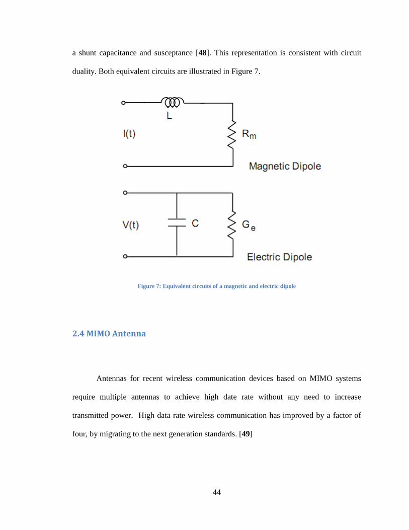
44
a shunt capacitance and susceptance [48]. This representation is consistent with circuit
duality. Both equivalent circuits are illustrated in Figure 7.
Figure 7: Equivalent circuits of a magnetic and electric dipole
2.4 MIMO Antenna
Antennas for recent wireless communication devices based on MIMO systems
require multiple antennas to achieve high date rate without any need to increase
transmitted power. High data rate wireless communication has improved by a factor of
four, by migrating to the next generation standards. [49]
45
2.4.1 Multiple Antennas
Recent research on wireless communication systems has shown that using
multiple antennas at both the transmitter and the receiver offers the possibility of higher
data rates compared to single antenna-systems. The information-theoretic capacity of
MIMO channels was shown to grow linearly with the minimum number of transmits and
receives antennas in rich scattering environments and at sufficiently high signal-to-noise
(SNR) ratios [50]. However, for single-input single-output (SISO) channels, the capacity
increases logarithmically with SNR. Thus, a significant capacity increase can be achieved
using MIMO systems without any increase in transmit power or expansion in the
bandwidth [51]. The earliest ideas in this field go back to work by A.R. Kaye and D.A.
George (1970) and W. van Etten (1975, 1976). Jack Winters and Jack Salz at Bell
Laboratories published several papers on beamforming related applications in 1984 and
1986 [52].
MIMO Techniques
1. Beamforming
2. Diversity
3. Multiplexing

46
The important techniques used in MIMO technology to enhance the data transfer
process are: Beamforming, Diversity and Multiplexing. Brief description of each
technique is as follows:
1. Beamforming
It is an effective technique for reducing the multiple-access interference,
where the antenna gain is increased in the direction of the desired user, whilst
reducing the gain towards the interfering users [53]. If the directions of the
different propagation paths are known at the transmitter or the receiver, then
beamforming techniques can be employed in order to direct the received beam
pattern in the direction of the specified antenna or user [54] [55]. Hence,
significant SNR gains can be achieved in comparison to a single-antenna
system. On the transmitter side, when the direction of arrival (DOA) of the
dominant paths at the receiver is known for the transmitter, then the transmit
power is concentrated in the direction of the target user, and less power is
wasted in the other directions. On the other hand, beamforming can be used in
order to reduce the co-channel interference or multi-user interference [53].
When using beamforming, each user adjusts their beam pattern to ensure that
there are nulls in the directions of the other users, while there is a high
directivity in the direction of the desired receiver. Hence, the system attains an
SNR gain.
There are many methods to achieve beamforming, such of these methods are:
47
a) Phased Array Antenna
A phased array antenna is composed of many radiating elements each with a
phase shifter. Beams are formed by shifting the phase of the signal emitted from each
radiating element, to provide constructive/destructive interference so as to steer the
beams in the desired direction. [56]
The main beam always points in the direction of the increasing phase shift. Well,
the beam direction can be electronically adjusted if the signal to be radiated is delivered
through an electronic phase shifter giving a continuous phase shift. However, this cannot
be extended unlimitedly. The highest value, which can be achieved for the Field of View
(FOV) of a phased array antenna is 120° (60° left and 60° right). With the sine theorem
the necessary phase moving can be calculated. [56]
Frequency Scanning Array
Frequency scanning is a special case of the phased array antenna where the main
beam steering occurs by the frequency scanning of the exciter. The beam steering is a
function of the transmitted frequency. This type of antenna is called a frequency scanning
array. The normal arrangement is to feed the different radiating elements from one folded
waveguide. The frequency scanning array is a special case of serial feeding type of a
phased array antenna and is based on a particular property of wave propagation in
waveguides. The phase difference between two radiating elements is n·360° at the normal
frequency. [56]

48
By varying the frequency, the angle between the axis of the main beam and the
normal on the array antenna changes. Height information is generated using the following
philosophy:
If the transmitted frequency rises then the beam travels up the face of the antenna;
If the transmitted frequency falls then the beam travels down the face of the
antenna.
b) Adaptive Antennas
In adaptive antenna systems multiple antennas are used to receive (or transmit)
the same information. Instead of using only one antenna to receive (or transmit) the radio
signal, combinations of multiple antennas output (or input) are used to focus the energy
towards one direction. The adequate combination of the signals received by the different
antennas results in a better link quality for a given transmitted power, or a lower
transmitted power required for a given link quality [57]. The same concept of adaptive
antennas can be found under different names such as smart antennas, or adaptive
beamforming [58]. The basic concept behind adaptive antennas is to change the standard
antenna that has an omnidirectional radiation pattern for a new one with a directive
radiation pattern that is continuously adapted to the environment [57], by changing the
amplitudes and phases from different array elements according to a real time criteria to
focus the beam towards a specific spatial direction.
49
c) Null Steering Techniques
The objective of steering nulls in the antenna array pattern in a particular direction
is to reduce the interference arriving in that direction. This can be achieved by controlling
the amplitude and/or phase of the current induced on the elements of the array or by
controlling the position of the elements of the array such that the array factor in that
direction is zero (practically to a required depth e.g. -60 dB with respect to the
normalized maximum array factor of 0 dB). This reduction is necessary in today's mobile
communication environment in order to face the various sources of interferences like Co-
Channel interference, Adjacent channel interference etc. Null steering involving the
above mentioned controllable variables is briefed below.
i) Element positive perturbation method
This technique was developed by Ismail and Dawoud [59], where null steering is
carried out by controlling the positions of the antenna array elements. This avoids the
complicated use of amplitude and/or phase control systems and frees the phase shifters
merely for steering the main beam towards the direction of the desired signal. An
experimental verification was done in [60] wherein, null steering was achieved for an
eight-element monopole over a ground plane. Single and double nulls were realized in the
side lobe region. Dawoud et al [61] applied genetic algorithm and compared the results
with analytical solution for array pattern nulling by element position perturbation. Null
steering in scanned arrays by using position perturbations was carried out in [62].
50
ii) Amplitude Only Control Method
In this method the amplitude of the induced currents are controlled to achieve
Null Steering. Mismer and Ismail [63] employed the method of amplitude only control to
perform null steering by a linear programming technique using minmax approximation.
Liao and Chu [64] investigated the technique to steer the array nulls for planar arrays by
controlling only the excitation current amplitudes based on genetic algorithms.
Implementation was done in rectangular and circular planar mays.
iii) Phase only control method
In this method, only the phases of the currents induced on the elements are varied.
Liao and Chu [65] used phase only null steering in hear arrays using a modified genetic
algorithm to speed up the convergence rate. Numerical results for 20-element linear array
with one to four imposed interferences were demonstrated. Ismail and Mismer [66]
presented a new antenna configuration of dual phase shifters to steer multiple nulls by
controlling the arbitrary phase perturbations. Steyskal demonstrated pattern nulling by
phase perturbations in [67]. Complex weight control method. Here pattern synthesis is
carried out by perturbing both phase and amplitude of the array elements. This is much
efficient technique. The number of degrees of freedom in this case is twice the number of
array elements resulting in better control of null steering. Mitchell et al [58] carried out
array pattern synthesis with performance constraints in complex plane where genetic
51
algorithm was applied on the roots of the array polynomial. Also, Compton et a1 [55]
presented a numerical technique to arrive at the complex weights, which gives a desired
side lobe level in linear arrays.
2. Diversity Coding
Techniques are used when there is no channel knowledge at the transmitter. In
diversity methods a single stream is transmitted, but the signal is coded using
techniques called space-time coding. The signal is emitted from each of the
transmit antennas with full or near orthogonal coding. Diversity coding
exploits the independent fading in the multiple antenna links to enhance signal
diversity. Because there is no channel knowledge, there is no beamforming or
array gain from diversity coding.
3. Spatial multiplexing
Spatial multiplexing requires MIMO antenna configuration. In spatial
multiplexing, a high rate signal is split into multiple lower rate streams and
each stream is transmitted from a different transmit antenna in the same
frequency channel. If these signals arrive at the receiver antenna array with
sufficiently different spatial signatures, the receiver can separate these
streams, re-creating parallel channels. Spatial multiplexing is a very powerful
technique for increasing channel capacity at higher signal-to-noise ratios
52
(SNR). The maximum number of spatial streams is limited by the number of
antennas at the transmitter or receiver. Spatial multiplexing can be used with
or without transmit channel knowledge.
Diversity MIMO vs. Multiplexing MIMO
The spatial freedom introduced by a MIMO system can be used in two distinct
ways [68] [69], i.e., either to improve link quality (diversity MIMO) or to enhance
throughput (multiplexing MIMO). Diversity MIMO schemes in general can increase the
performance by exploit array gain and/or diversity gain, but it will have the same data
rate as the SISO system, e.g. Space-time coding. On the other hand, multiplexing MIMO
can increase the symbol data rate at no cost of extra spectrum. So, there are two methods
widely used for transmitting MIMO data. If the channel has a negligible error rate, we
can send several data simultaneously over multiple antennas. This is known as spatial
multiplexing, which utilizes the spectrum very efficiently. In contrast, if the environment
has high error rate, we transmit the same data over multiple antennas. This is called as
space-time coding. The purpose of this approach is to increase the diversity of MIMO to
combat signal fading.
2.4.2 Antenna Array
Often in wireless devices with single element antennas are unable to meet the gain
or radiation pattern requirements. Combining several single antenna elements in an array
can be a possible solution.
53
Definition
An array of antenna elements is a spatially extended collection of N similar
radiators or elements, where N is a countable number bigger than 1, and the term "similar
radiators" means that all the elements have the same polar radiation patterns, orientated in
the same direction in 3-d space. Typically, the elements are spaced on a regular grid and
fed with the same frequency and same or progressed amplitude and phase angle.
Types of Antenna Arrays
There are a few different general types of antenna arrays. When the array is
arranged in a straight line this is called a linear array. Antennas are arranged in parallel
lines on one plane has a plane array in two dimensions. Many planes in a group of arrays
or antennas results in a three dimensional array. An antenna array may consist of a
group of Omni-directional radiators. Or, the array may have a group of radiators that are
identical. In a group of identical radiators all the antennas must be share the same
orientation in space. The same orientation results in the desired effect of reinforcement or
cancellation of the electric field intensity. The same orientation ensures polarization in
the same direction in space. [70]
54
Antenna arrays, radiation pattern and array factor
The antenna elements can be arranged to form a 1 or 2 dimensional antenna array.
A number of antenna array specific aspects will be outlined; We used 1dimensional
arrays for simplicity reasons. Antennas exhibit a specific radiation pattern. The overall
radiation pattern changes when several antenna elements are combined in an array. This
is due to the so called array factor: this factor quantifies the effect of combining radiating
elements in an array without the element specific radiation pattern taken into account.
The overall radiation pattern of an array is determined by this array factor combined with
the radiation pattern of the antenna element. The overall radiation pattern results in a
certain directivity and thus gain linked through the efficiency with the directivity.
Directivity and gain are equal if the efficiency is 100%.
Broadside vs. end fire arrays
Arrays can be designed to radiate in either Broadside i.e. Radiation perpendicular
to array orientation or End Fire i.e. Radiation in the same direction as the array
orientation. The array factor depends on the number of elements, the element spacing,
amplitude and phase of the applied signal to each element. The number of elements and
the element spacing determine the surface area of the overall radiating structure. This
55
surface area is called aperture. A larger aperture results in a higher gain. The aperture
efficiency quantifies how efficient the aperture is used.
Feed network of the array
The individual antenna elements in an array are fed using a feed network. The
complexity of the feed network depends on the number of elements, the amplitude and/or
phase distribution between the elements, the ability to do beam steering. It is important to
realize that the feed network is the most complex part of the array. A detailed design
process of a linear 2-element array for MIMO application is described in chapter 4.

56
CHAPTER 3
Design of an Electrically Small Antenna
As previously mentioned, meander line technology is adopted for the single
element antenna because this type of antennas could have much smaller area than other
types of antennas listed in Table 4. In this section we will present the design of an
antenna element that will fit a size of 20x40 mm2 with a resonant frequency of 780 MHz,
and at least 40 MHz of bandwidth and 0 dB of gain with a radiation pattern that covers
around a cell phone.
3.1 Empirical Design of a Meander Line Antenna
One way of designing a meander line antenna is by using the empirical equation
mentioned in [21], which represents every dimension needed in the design in term of the
wavelength and actually the effective wavelength
The design procedure of a meander antenna using empirical formulas can be summarized
as:

57
1. First determine the type and dielectric constant of the substrate and the operating
frequency that you want your antenna to work on.
2. Find the dimensions of your MLA using these equations, see Figure 8:
eff
eff
eff
eff
0.16* (3.1)
s=0.42* (3.2)
l=0.70* (3.3)
w=0.05* (3.4)
d
where, d is the width of the meander line arm, s is the length of the meander line arm, l
is the length of the meander line, w is the width of the meander line, eff is the effective
wavelength of the substrate and is given by
0eff (3.5)
reff
Where, 0 is the free space wavelength and is the effective dielectric constant
3. Find reff using:
1
21 11 10 (3.6)
2 2
r r
reff
h
w
Where, h is the height of substrate, r is the dielectric constant of given material, w is the
width of meander line antenna.
Applying 3.1-3.6, and using a resonant frequency of 780 MHz, FR-4 material ( 4.4r )
and substrate thickness of 1.6 mm, we get
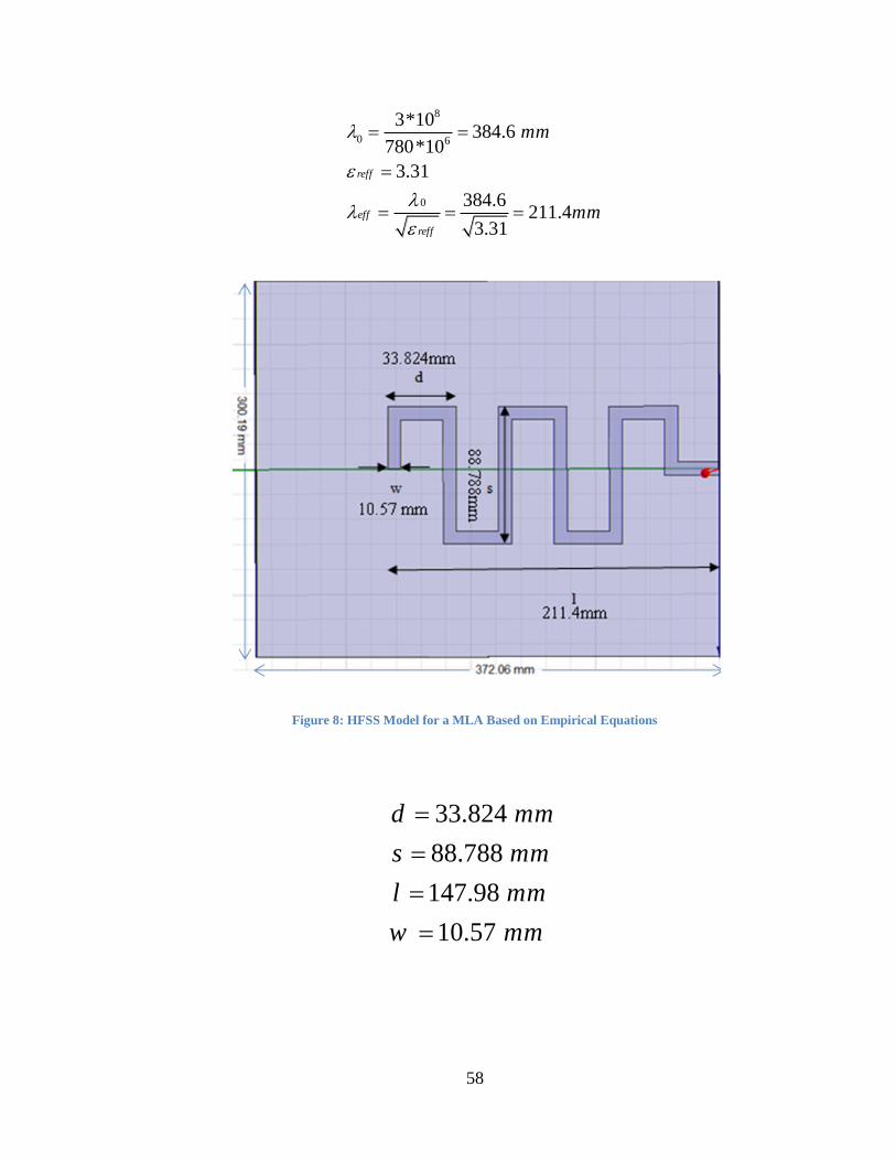
58
8
0 6
0
3*10384.6
780*10
3.31
384.6211.4
3.31
reff
eff
reff
mm
mm
Figure 8: HFSS Model for a MLA Based on Empirical Equations
33.824
88.788
147.98
10.57
d mm
s mm
l mm
w mm
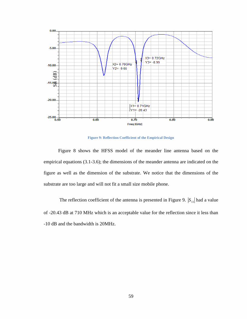
59
Figure 9: Reflection Coefficient of the Empirical Design
Figure 8 shows the HFSS model of the meander line antenna based on the
empirical equations (3.1-3.6); the dimensions of the meander antenna are indicated on the
figure as well as the dimension of the substrate. We notice that the dimensions of the
substrate are too large and will not fit a small size mobile phone.
The reflection coefficient of the antenna is presented in Figure 9. 11S had a value
of -20.43 dB at 710 MHz which is an acceptable value for the reflection since it less than
-10 dB and the bandwidth is 20MHz.
S11
(d
B)
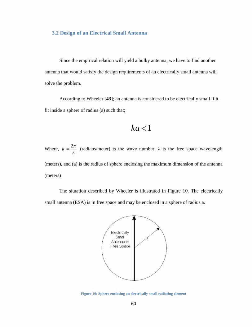
60
3.2 Design of an Electrical Small Antenna
Since the empirical relation will yield a bulky antenna, we have to find another
antenna that would satisfy the design requirements of an electrically small antenna will
solve the problem.
According to Wheeler [43]; an antenna is considered to be electrically small if it
fit inside a sphere of radius (a) such that;
1ka
Where, 2
k
(radians/meter) is the wave number, λ is the free space wavelength
(meters), and (a) is the radius of sphere enclosing the maximum dimension of the antenna
(meters)
The situation described by Wheeler is illustrated in Figure 10. The electrically
small antenna (ESA) is in free space and may be enclosed in a sphere of radius a.
Figure 10: Sphere enclosing an electrically small radiating element

61
There are several types of ESA. In this work we use a meander line ESA. This
design is based on that presented in [23] but that design has an operating frequency of
1.575 GHz which is almost double the operating frequency that we need, so we need to
re-design the antenna to operate at 780 MHz with a size that satisfies the dimension
constraints of our design.
Since MLAs do not have a specific design procedure, a study on the variation of
the parameters is conducted to determine the antenna dimensions. First we determine the
size of the substrate we need, then we model the meander line antenna on the top of the
substrate with the ground plane on the bottom face of it and start vary the parameters to
know its effect on the operating frequency, these parameters are thickness of the
substrate, dielectric constant, width and length of the meander antenna arms, spacing
between these arms, number of turns, width of the matching line, length of the ground
plane, width of the meander line and the distance between the last arm and the edge of the
substrate and section 3.3 investigate some of these parameters with more details.
Figure 11 shows the schematic diagram of the designed meander line ESA with
parameter values given in the Table 4.
Table 4: Specifications of our Designed Antenna
Frequency
Dielectric
Constant
NO. of
Turns
Substrate
Thickness
Substrate
Length
Substrate
Width
780 MHz 4.4 4 1.6 mm 40 mm 20 mm
W2 W3 W4 W5 Lg L1 L2 S
1.651 mm 1 mm 1 mm 1 mm 16.4 mm 12.27 mm 5.925 mm 15.5 mm
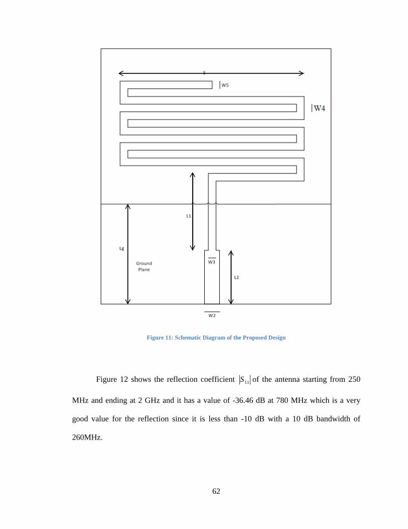
62
Figure 11: Schematic Diagram of the Proposed Design
Figure 12 shows the reflection coefficient 11S of the antenna starting from 250
MHz and ending at 2 GHz and it has a value of -36.46 dB at 780 MHz which is a very
good value for the reflection since it is less than -10 dB with a 10 dB bandwidth of
260MHz.
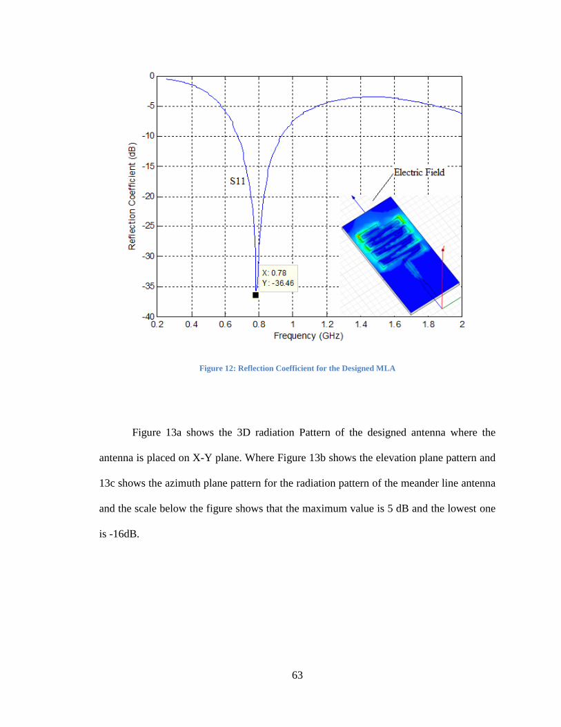
63
Figure 12: Reflection Coefficient for the Designed MLA
Figure 13a shows the 3D radiation Pattern of the designed antenna where the
antenna is placed on X-Y plane. Where Figure 13b shows the elevation plane pattern and
13c shows the azimuth plane pattern for the radiation pattern of the meander line antenna
and the scale below the figure shows that the maximum value is 5 dB and the lowest one
is -16dB.
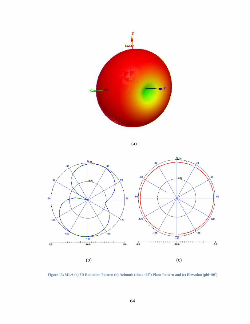
64
(a)
(b) (c)
Figure 13: MLA (a) 3D Radiation Pattern (b) Azimuth (theta=900) Plane Pattern and (c) Elevation (phi=900)
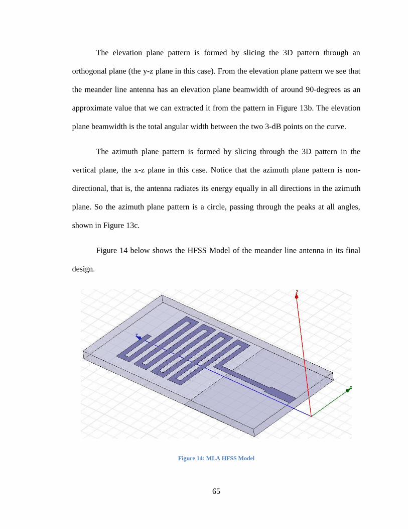
65
The elevation plane pattern is formed by slicing the 3D pattern through an
orthogonal plane (the y-z plane in this case). From the elevation plane pattern we see that
the meander line antenna has an elevation plane beamwidth of around 90-degrees as an
approximate value that we can extracted it from the pattern in Figure 13b. The elevation
plane beamwidth is the total angular width between the two 3-dB points on the curve.
The azimuth plane pattern is formed by slicing through the 3D pattern in the
vertical plane, the x-z plane in this case. Notice that the azimuth plane pattern is non-
directional, that is, the antenna radiates its energy equally in all directions in the azimuth
plane. So the azimuth plane pattern is a circle, passing through the peaks at all angles,
shown in Figure 13c.
Figure 14 below shows the HFSS Model of the meander line antenna in its final
design.
Figure 14: MLA HFSS Model

66
Now we need to prove that our antenna is indeed an electrically small antenna.
First condition for antenna to be considered as ESA is (ka<1)
1
211.4
20.0297 /
133.645
ka
mm
k rad mm
a mmk
According to our antenna it can be fit inside a sphere of radius 22.36 a mm
0.0297*22.36 0.665ka
We can see that (ka) is less than one and this 0.78 GHz meander line antenna is by
definition an electrically small antenna. This antenna is known to be linear and polarized
vertical to the ground plane so we easily calculate the radiation Q [71]
31 1
4.91125 (3.7)LQka ka
The actual value of the bandwidth is
33.33%c
BWBW
f
The approximate bandwidth for an RLC type circuit in terms of Q is:
1 (3.8)
*
SBW
Q S
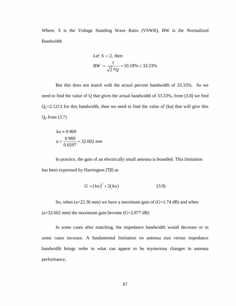
67
Where, S is the Voltage Standing Wave Ratio (VSWR), BW is the Normalized
Bandwidth
2,
110.18% 33.33%
2 *
Let S then
BWQ
But this does not match with the actual percent bandwidth of 33.33%. So we
need to find the value of Q that gives the actual bandwidth of 33.33%, from (3.8) we find
QL=2.1213 for this bandwidth, then we need to find the value of (ka) that will give this
QL from (3.7)
0.969
0.96932.602
0.0297
ka
a mm
In practice, the gain of an electrically small antenna is bounded. This limitation
has been expressed by Harrington [72] as
2
2 (3.9)G ka ka
So, when (a=22.36 mm) we have a maximum gain of (G=1.74 dB) and when
(a=32.602 mm) the maximum gain become (G=2.877 dB)
In some cases after matching, the impedance bandwidth would decrease or in
some cases increase. A fundamental limitation on antenna size versus impedance
bandwidth brings order to what can appear to be mysterious changes in antenna
performance.
68
3.3 Parameters Variation
There are many parameters that need to be investigated in order to have a general
view of the effect of every parameter and these parameters are:
3.3.1 Dielectric Permittivity (𝜺𝒓)
FR-4 glass epoxy is a popular and versatile high pressure thermoset plastic
laminate grade with good strength to weight ratios. With near zero water absorption FR-4
is most commonly used as an electrical insulator possessing considerable mechanical
strength. The material is known to retain its high mechanical values and electrical
insulating qualities in both dry and humid conditions. These attributes, along with good
fabrication characteristics, lend utility to this grade for a wide variety of electrical and
mechanical applications.
Dielectric constant or permittivity 𝜺𝒓 for this material has a minimum value of
(4.0) and a maximum value of (4.8). [73]
Table 5: Dielectric Permittivity Effect on the Design
4 0.78 -32.52 240
4.4 0.78 -30.9 260
4.8 0.77 -31.68 260

69
In Table 5 above, it shows different dielectric constant values for the same FR-4
material and the corresponding center frequency, reflection coefficient and bandwidth.
We notice that the resonant frequency decreases as the dielectric constant increase.
3.3.2 Spacing Between MLA Arms
The spacing (W4 in figure 11) between two bends is very critical, where if the
bends are too close to each other, then cross coupling will be more, which affects the
polarization purity of the resultant radiation pattern.
In other case the spacing is limited due to the available array grid space and also
the polarization of the radiated field will vary with the spacing between the bends, and
the spacing between the microstrip lines. The present meander line structure is designed
with liner polarization with less cross coupling between the bends, to fit within the
available array grid size.
The following three figures show the effect of spacing on frequency, reflection
coefficient and on bandwidth. We notice from figure 15 that as the spacing between
meander line arms increased the center frequency will reduce, while figure 16 shows the
effect of spacing on the reflection coefficient and we can see that as the spacing increased
until a certain value the reflection coefficient will be further improved and if it is
increased more than that the reflection will reduce but it is still gives a good reflection.
Figure 17 shows the relationship between the spacing and bandwidth and it is obvious to
notice that as the spacing increased the bandwidth will reduce, which is almost same
relation as with the frequency.

70
Figure 15: Effect of Spacing on Center Frequency
Figure 16: Effect of Spacing on Reflection Coefficient
0.5 0.6 0.7 0.8 0.9 1 1.1 1.2 1.3 1.4 1.50.5
0.55
0.6
0.65
0.7
0.75
0.8
0.85
0.9
0.95
1
Spacing (mm)
Fre
quency (
GH
z)
0.5 0.6 0.7 0.8 0.9 1 1.1 1.2 1.3 1.4 1.5-50
-45
-40
-35
-30
-25
-20
-15
Spacing (mm)
Reflection C
oeff
icie
nt
(dB
)
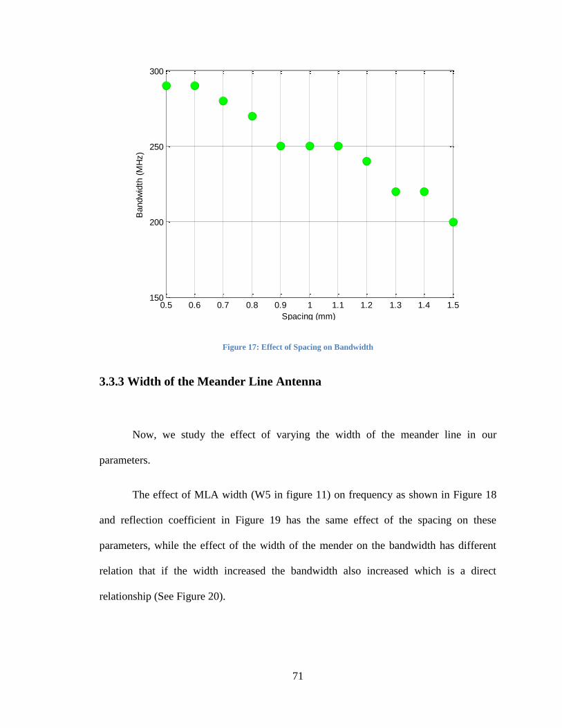
71
Figure 17: Effect of Spacing on Bandwidth
3.3.3 Width of the Meander Line Antenna
Now, we study the effect of varying the width of the meander line in our
parameters.
The effect of MLA width (W5 in figure 11) on frequency as shown in Figure 18
and reflection coefficient in Figure 19 has the same effect of the spacing on these
parameters, while the effect of the width of the mender on the bandwidth has different
relation that if the width increased the bandwidth also increased which is a direct
relationship (See Figure 20).
0.5 0.6 0.7 0.8 0.9 1 1.1 1.2 1.3 1.4 1.5150
200
250
300
Spacing (mm)
Bandw
idth
(M
Hz)

72
Figure 18: The effect of Varying the MLA Width on Frequency
Figure 19: The effect of Varying the MLA Width on Reflection Coefficient
0.5 0.6 0.7 0.8 0.9 1 1.1 1.2 1.3 1.4 1.50.5
0.55
0.6
0.65
0.7
0.75
0.8
0.85
0.9
0.95
1
MLA Width (mm)
Fre
quency (
GH
z)
0.5 0.6 0.7 0.8 0.9 1 1.1 1.2 1.3 1.4 1.5-50
-45
-40
-35
-30
-25
-20
-15
MLA Width (mm)
Reflection C
oeff
icie
nt
(dB
)
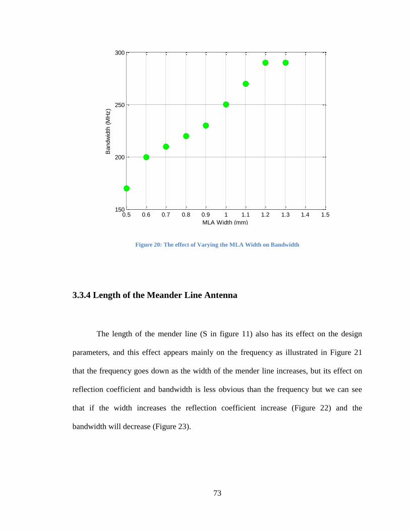
73
Figure 20: The effect of Varying the MLA Width on Bandwidth
3.3.4 Length of the Meander Line Antenna
The length of the mender line (S in figure 11) also has its effect on the design
parameters, and this effect appears mainly on the frequency as illustrated in Figure 21
that the frequency goes down as the width of the mender line increases, but its effect on
reflection coefficient and bandwidth is less obvious than the frequency but we can see
that if the width increases the reflection coefficient increase (Figure 22) and the
bandwidth will decrease (Figure 23).
0.5 0.6 0.7 0.8 0.9 1 1.1 1.2 1.3 1.4 1.5150
200
250
300
MLA Width (mm)
Bandw
idth
(M
Hz)
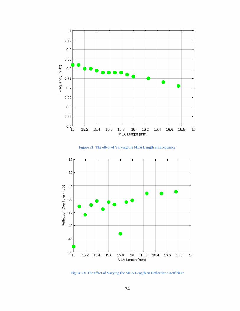
74
Figure 21: The effect of Varying the MLA Length on Frequency
Figure 22: The effect of Varying the MLA Length on Reflection Coefficient
15 15.2 15.4 15.6 15.8 16 16.2 16.4 16.6 16.8 170.5
0.55
0.6
0.65
0.7
0.75
0.8
0.85
0.9
0.95
1
MLA Length (mm)
Fre
quency (
GH
z)
15 15.2 15.4 15.6 15.8 16 16.2 16.4 16.6 16.8 17-50
-45
-40
-35
-30
-25
-20
-15
MLA Length (mm)
Reflection C
oeff
icie
nt
(dB
)
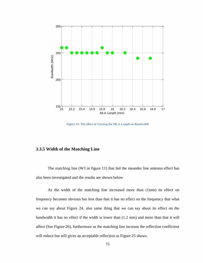
75
Figure 23: The effect of Varying the MLA Length on Bandwidth
3.3.5 Width of the Matching Line
The matching line (W3 in figure 11) that fed the meander line antenna effect has
also been investigated and the results are shown below
As the width of the matching line increased more than (1mm) its effect on
frequency becomes obvious but less than that it has no effect on the frequency that what
we can say about Figure 24, also same thing that we can say about its effect on the
bandwidth it has no effect if the width is lower than (1.2 mm) and more than that it will
affect (See Figure 26), furthermore as the matching line increase the reflection coefficient
will reduce but still gives an acceptable reflection as Figure 25 shows.
15 15.2 15.4 15.6 15.8 16 16.2 16.4 16.6 16.8 17150
200
250
300
MLA Length (mm)
Bandw
idth
(M
Hz)
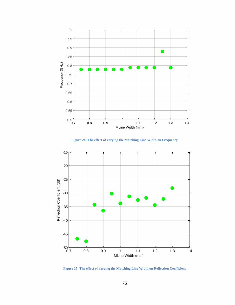
76
Figure 24: The effect of varying the Matching Line Width on Frequency
Figure 25: The effect of varying the Matching Line Width on Reflection Coefficient
0.7 0.8 0.9 1 1.1 1.2 1.3 1.40.5
0.55
0.6
0.65
0.7
0.75
0.8
0.85
0.9
0.95
1
MLine Width (mm)
Fre
quency (
GH
z)
0.7 0.8 0.9 1 1.1 1.2 1.3 1.4-50
-45
-40
-35
-30
-25
-20
-15
MLine Width (mm)
Reflection C
oeff
icie
nt
(dB
)
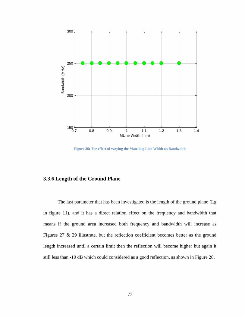
77
Figure 26: The effect of varying the Matching Line Width on Bandwidth
3.3.6 Length of the Ground Plane
The last parameter that has been investigated is the length of the ground plane (Lg
in figure 11), and it has a direct relation effect on the frequency and bandwidth that
means if the ground area increased both frequency and bandwidth will increase as
Figures 27 & 29 illustrate, but the reflection coefficient becomes better as the ground
length increased until a certain limit then the reflection will become higher but again it
still less than -10 dB which could considered as a good reflection, as shown in Figure 28.
0.7 0.8 0.9 1 1.1 1.2 1.3 1.4150
200
250
300
MLine Width (mm)
Bandw
idth
(M
Hz)
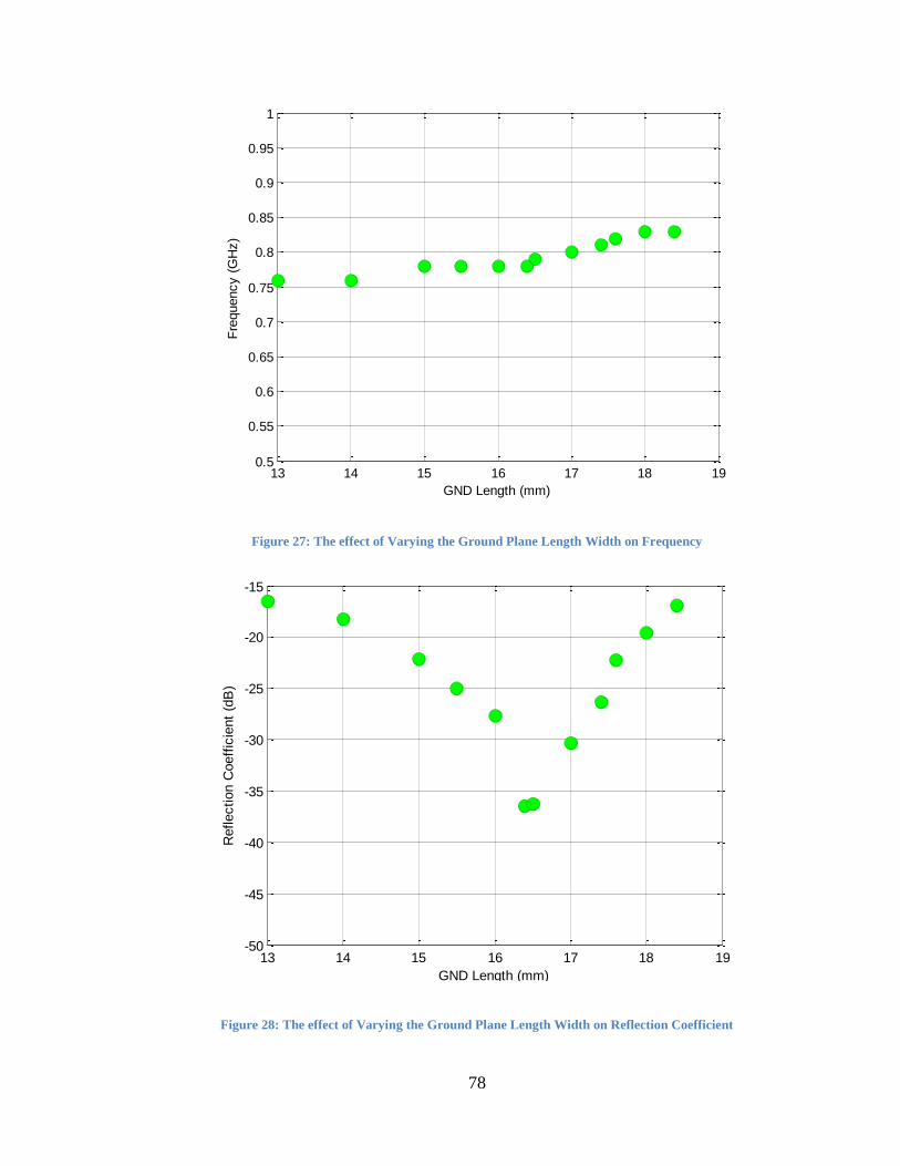
78
Figure 27: The effect of Varying the Ground Plane Length Width on Frequency
Figure 28: The effect of Varying the Ground Plane Length Width on Reflection Coefficient
13 14 15 16 17 18 190.5
0.55
0.6
0.65
0.7
0.75
0.8
0.85
0.9
0.95
1
GND Length (mm)
Fre
quency (
GH
z)
13 14 15 16 17 18 19-50
-45
-40
-35
-30
-25
-20
-15
GND Length (mm)
Reflection C
oeff
icie
nt
(dB
)
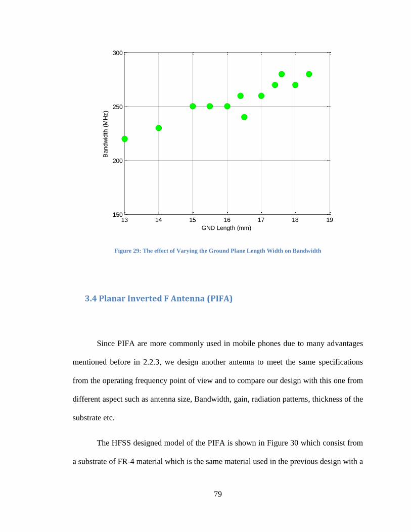
79
Figure 29: The effect of Varying the Ground Plane Length Width on Bandwidth
3.4 Planar Inverted F Antenna (PIFA)
Since PIFA are more commonly used in mobile phones due to many advantages
mentioned before in 2.2.3, we design another antenna to meet the same specifications
from the operating frequency point of view and to compare our design with this one from
different aspect such as antenna size, Bandwidth, gain, radiation patterns, thickness of the
substrate etc.
The HFSS designed model of the PIFA is shown in Figure 30 which consist from
a substrate of FR-4 material which is the same material used in the previous design with a
13 14 15 16 17 18 19150
200
250
300
GND Length (mm)
Bandw
idth
(M
Hz)

80
dielectric constant of 4.4 and large ground plane with area of 30x80mm2 and a patch
antenna with area of 30x22mm2 and a shorting pin and feeding point as shown in the
figure. Table 6 summarizes the specifications for this antenna.
Figure 31 shows the reflection coefficient of this antenna that operates at our
required frequency with a value of -22.59 dB and has a band width of 20 MHz, and the
3D radiation pattern is shown in Figure 32.
Figure 30: HFSS Model for the PIFA Antenna
Table 6: PIFA Specifications
Frequency S11 Bandwidth Width Length Thickness
780 MHz -22.59 dB 20 MHz 30 mm 80 mm 10 mm
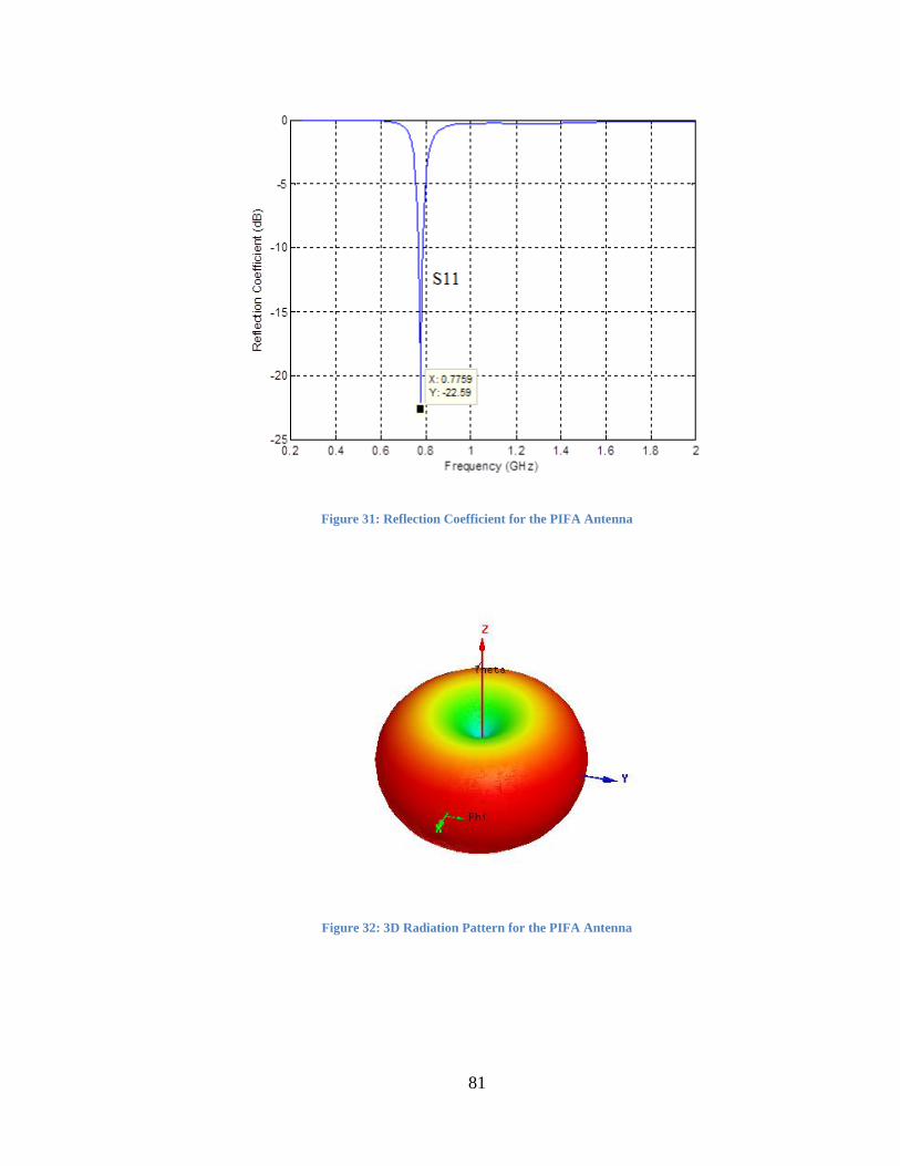
81
Figure 31: Reflection Coefficient for the PIFA Antenna
Figure 32: 3D Radiation Pattern for the PIFA Antenna
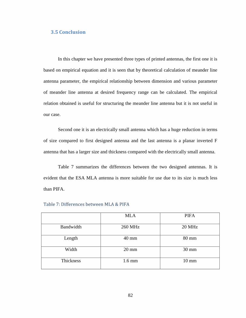
82
3.5 Conclusion
In this chapter we have presented three types of printed antennas, the first one it is
based on empirical equation and it is seen that by theoretical calculation of meander line
antenna parameter, the empirical relationship between dimension and various parameter
of meander line antenna at desired frequency range can be calculated. The empirical
relation obtained is useful for structuring the meander line antenna but it is not useful in
our case.
Second one it is an electrically small antenna which has a huge reduction in terms
of size compared to first designed antenna and the last antenna is a planar inverted F
antenna that has a larger size and thickness compared with the electrically small antenna.
Table 7 summarizes the differences between the two designed antennas. It is
evident that the ESA MLA antenna is more suitable for use due to its size is much less
than PIFA.
Table 7: Differences between MLA & PIFA
MLA PIFA
Bandwidth 260 MHz 20 MHz
Length 40 mm 80 mm
Width 20 mm 30 mm
Thickness 1.6 mm 10 mm

83
CHAPTER 4
Design of a MIMO Antenna System
The design of a multiple input and multiple output (MIMO) antenna for LTE
systems is presented here. The MIMO antenna comprises of a two element meander line
linear array. The designed antenna is optimized using HFSS simulator and the mutual
coupling between the antennas elements are improved using a novel technique. A
detailed overview of a MIMO and array antenna is presented in section 2.4.
4.1 Design of a 2 Element MIMO Antenna System
The design procedure of a MIMO antenna is presented in this section. The
designing consist of the 2 element meander line antenna (MLA), positioned reasonably
apart to satisfy the limitation related to antenna size and mutual coupling between
elements. The configurations of MIMO antennas investigated with four different
arrangements of the meander line elements are shown in Figures 33(a) to 36(a). The
reflection and isolation responses (S11, S22 and S21) of these configurations are plotted in
Figures 33(b) to 36(b), respectively. Note that in Figure 33(b), the reflection responses
(S11 and S22) of the MIMO configuration #1 demonstrate an impedance bandwidth of

84
25% with mutual isolation -7.10dB. Although the reflection response is acceptable, but
the isolation needed improvement.
(a)
Figure 33: (a) MIMO antenna configuration-#1 (b) S-parameter Responses
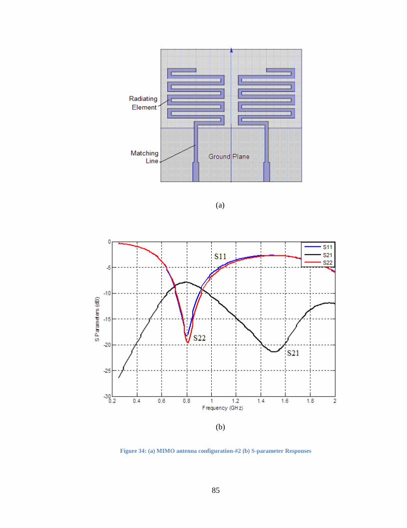
85
(a)
(b)
Figure 34: (a) MIMO antenna configuration-#2 (b) S-parameter Responses
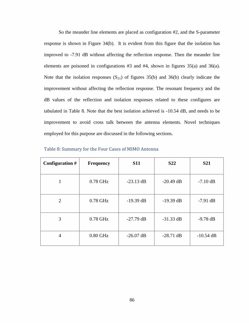
86
So the meander line elements are placed as configuration #2, and the S-parameter
response is shown in Figure 34(b). It is evident from this figure that the isolation has
improved to -7.91 dB without affecting the reflection response. Then the meander line
elements are poisoned in configurations #3 and #4, shown in figures 35(a) and 36(a).
Note that the isolation responses (S21) of figures 35(b) and 36(b) clearly indicate the
improvement without affecting the reflection response. The resonant frequency and the
dB values of the reflection and isolation responses related to these configures are
tabulated in Table 8. Note that the best isolation achieved is -10.54 dB, and needs to be
improvement to avoid cross talk between the antenna elements. Novel techniques
employed for this purpose are discussed in the following sections.
Table 8: Summary for the Four Cases of MIMO Antenna
Configuration # Frequency S11 S22 S21
1 0.78 GHz -23.13 dB -20.49 dB -7.10 dB
2 0.78 GHz -19.39 dB -19.39 dB -7.91 dB
3 0.78 GHz -27.79 dB -31.33 dB -9.78 dB
4 0.80 GHz -26.07 dB -28.71 dB -10.54 dB
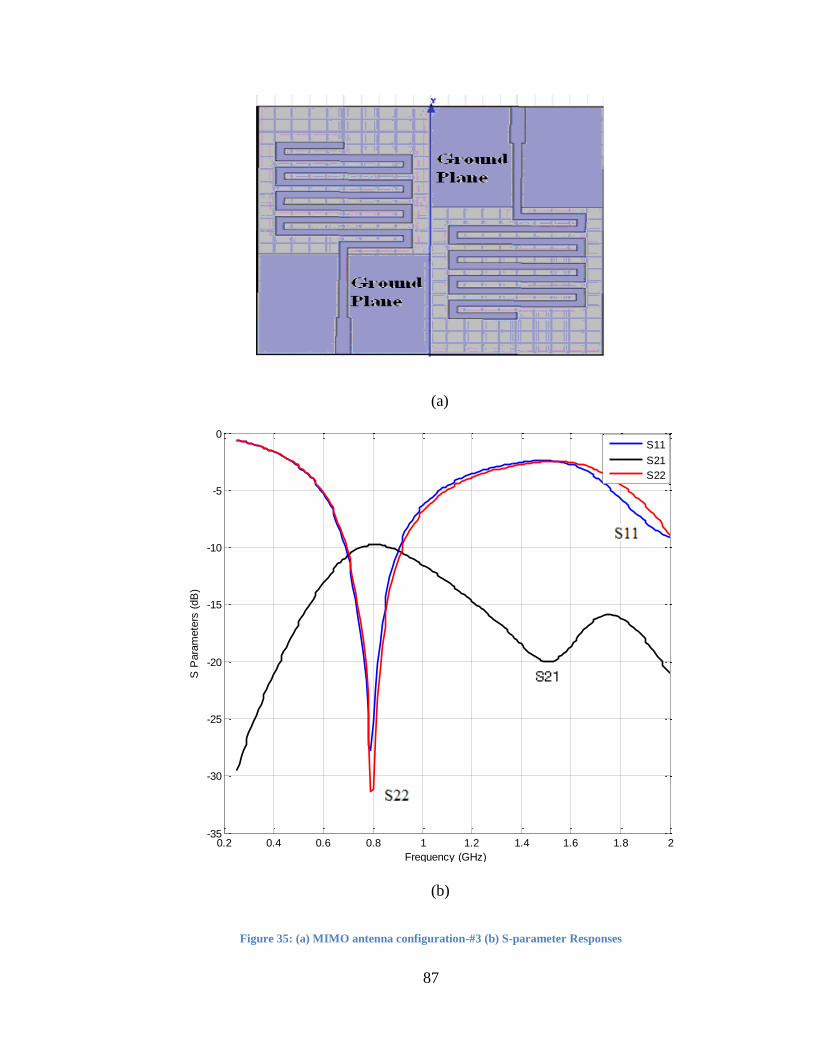
87
(a)
(b)
Figure 35: (a) MIMO antenna configuration-#3 (b) S-parameter Responses
0.2 0.4 0.6 0.8 1 1.2 1.4 1.6 1.8 2-35
-30
-25
-20
-15
-10
-5
0
Frequency (GHz)
S P
ara
mete
rs (
dB
)
S11
S21
S22
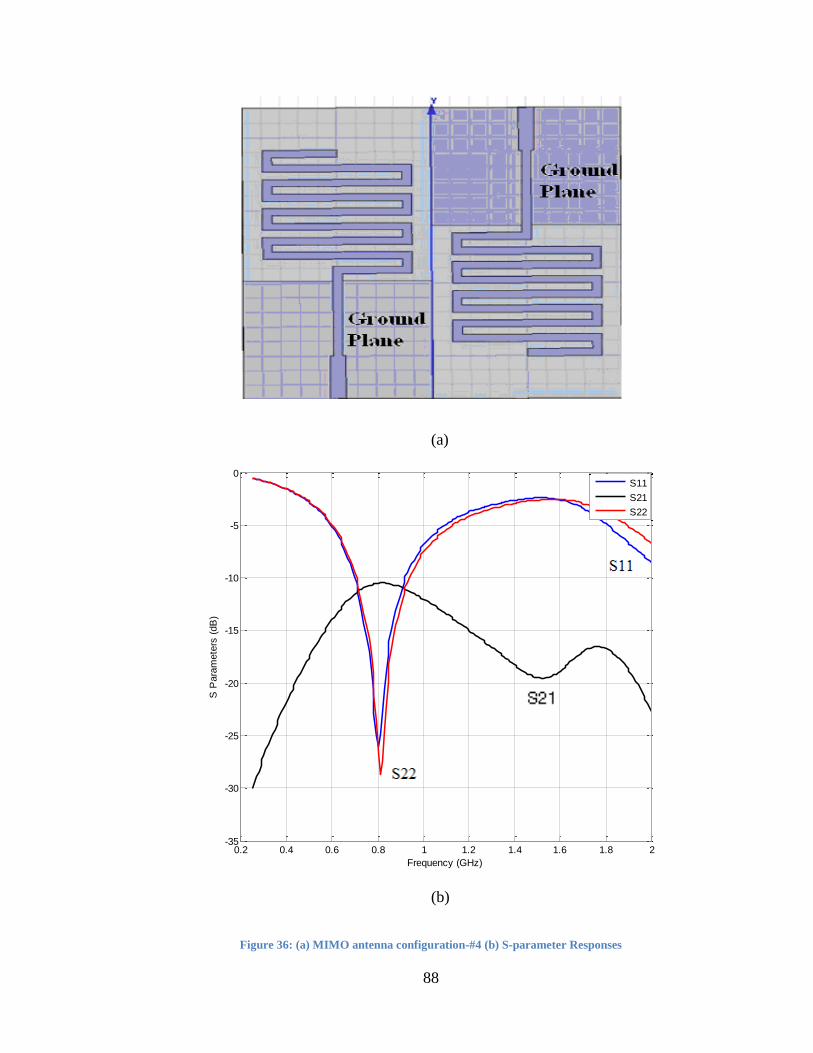
88
(a)
(b)
Figure 36: (a) MIMO antenna configuration-#4 (b) S-parameter Responses
0.2 0.4 0.6 0.8 1 1.2 1.4 1.6 1.8 2-35
-30
-25
-20
-15
-10
-5
0
Frequency (GHz)
S P
ara
mete
rs (
dB
)
S11
S21
S22

89
4.2 Improving Isolation between Antenna Elements
Novel techniques are discussed here section to improve the isolation or
correlation coefficient between the adjacent elements of the MIMO antenna. The first
method adopted here to improve the mutual coupling increases the separation between
the antenna elements. Figure 37 shows a MIMO antenna with antenna elements placed
apart from each other to reduce the isolation or mutual coupling. Figure 38 plots the
isolation with increasing substrate width, while the antenna elements are always placed at
the center of each side of the substrate. Note that this technique allows us to improve the
isolation up to -14.2dB. The improvement of isolation can be further improved by
increasing the substrate, while keeping the distant between the antenna and the substrate
edge constant. The isolation response for this case is shown in figure 39, where best
possible isolation is -22dB. Note that in both above cases, the isolation is improved at the
cost of the total size of the MIMO antenna, although they were kept within the limit of
LTE specifications.
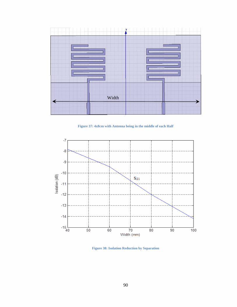
90
Figure 37: 4x8cm with Antenna being in the middle of each Half
Figure 38: Isolation Reduction by Separation
Width
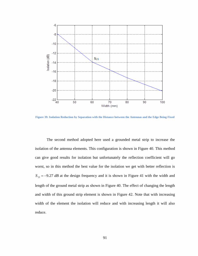
91
Figure 39: Isolation Reduction by Separation with the Distance between the Antennas and the Edge Being Fixed
The second method adopted here used a grounded metal strip to increase the
isolation of the antenna elements. This configuration is shown in Figure 40. This method
can give good results for isolation but unfortunately the reflection coefficient will go
worst, so in this method the best value for the isolation we get with better reflection is
21 9.27 S dB at the design frequency and it is shown in Figure 41 with the width and
length of the ground metal strip as shown in Figure 40. The effect of changing the length
and width of this ground strip element is shown in Figure 42. Note that with increasing
width of the element the isolation will reduce and with increasing length it will also
reduce.
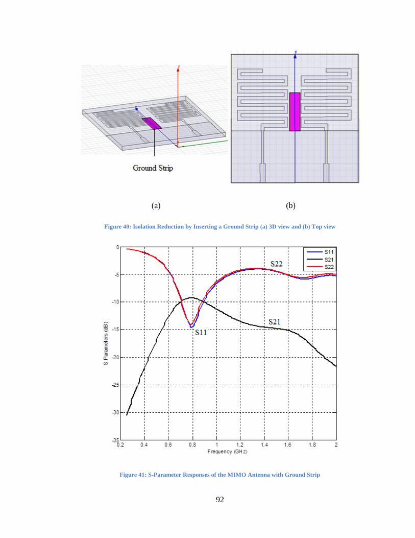
92
Figure 40: Isolation Reduction by Inserting a Ground Strip (a) 3D view and (b) Top view
Figure 41: S-Parameter Responses of the MIMO Antenna with Ground Strip
(a) (b)

93
Figure 42: Isolation verses width and Length of the Ground Strip
The third method to reduce isolation combined the first and second method. In
this method the separation between the edges of the antenna elements are varied in
addition to introducing a parasitic element between them. This antenna is shown in
Figure 43. The simulated reflection (S11, S22) and isolation (S21) responses are plotted in
Figure 44. Note that the isolation demonstrate by this configuration is -11.14 dB with an
impedance bandwidth of 27.71%.
0 0.5 1 1.5 2 2.5 3 3.5-18
-16
-14
-12
-10
-8
-6
Width of the Ground Strip (mm)
Isola
tion (
dB
)
L=23.805 mm
L=11.9025 mm
L=5.95125 mm
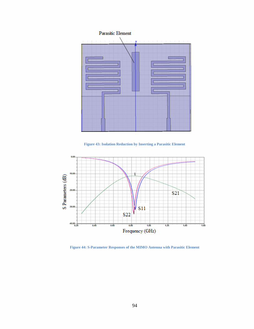
94
Figure 43: Isolation Reduction by Inserting a Parasitic Element
Figure 44: S-Parameter Responses of the MIMO Antenna with Parasitic Element
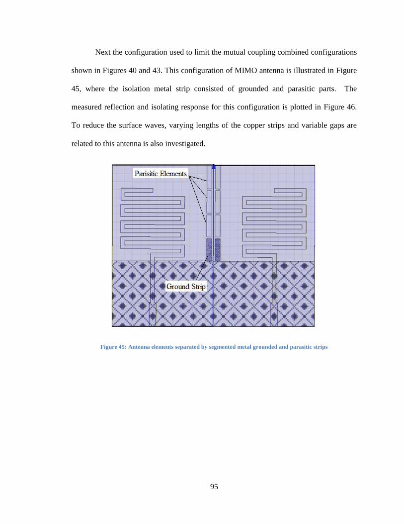
95
Next the configuration used to limit the mutual coupling combined configurations
shown in Figures 40 and 43. This configuration of MIMO antenna is illustrated in Figure
45, where the isolation metal strip consisted of grounded and parasitic parts. The
measured reflection and isolating response for this configuration is plotted in Figure 46.
To reduce the surface waves, varying lengths of the copper strips and variable gaps are
related to this antenna is also investigated.
Figure 45: Antenna elements separated by segmented metal grounded and parasitic strips

96
Figure 46: S-parameter responses of the MIMO antenna of figure 45.
The final novel method investigated here to reduce the isolation evolved from
above investigation and employed an L-shaped ground conductor for each meander line
antenna element. This configuration is shown in Figure 47 and demonstrates the expected
isolation between the antenna elements. The simulated s-parameters of this configuration
are plotted in Figure 48. Note that the isolation exhibited by this MIMO antenna is -20
dB and with impedance bandwidth of 23%. The radiation response of this antenna is also
simulated and plotted in Figure 49. Note that the 3D radiation plot in Figure 49(a) clearly
illustrates the doughnut shaped radiation pattern, as expected from this class of antenna.
The elevation and azimuth plane plots of this antenna are also shown in this figure. Note
that isolation between the antennas elements can further improved by superimposing the
separation technique illustrated in Figure 40 with the allowable antenna size of 40x100
mm2. The s-parameters of the design are tabulated in Table 9.

97
Table 9: Specification for the Two Element MIMO Antenna
Frequency S11 S22 S21
0.78 GHz -16.02 dB -16.11 dB -19.89 dB
Figure 47: HFSS Model for MIMO Antenna with Two L Shaped Ground Plane
Figure 48: S Parameters for the MIMO Antenna with Two L Shaped Ground Plane
0.2 0.4 0.6 0.8 1 1.2 1.4 1.6-45
-40
-35
-30
-25
-20
-15
-10
-5
0
Frequency (GHz)
S P
ara
mete
rs (
dB
)
S11
S21
S22
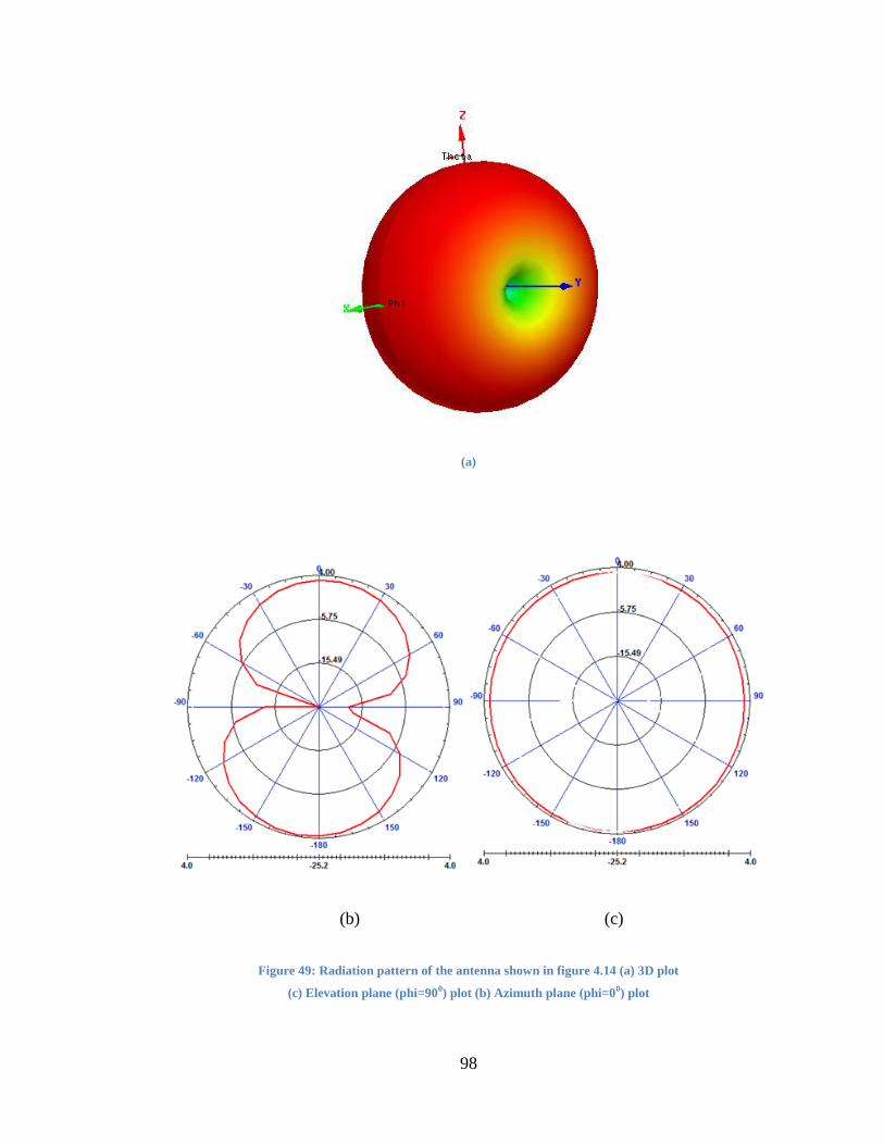
98
(a)
(b) (c)
Figure 49: Radiation pattern of the antenna shown in figure 4.14 (a) 3D plot
(c) Elevation plane (phi=900) plot (b) Azimuth plane (phi=00) plot
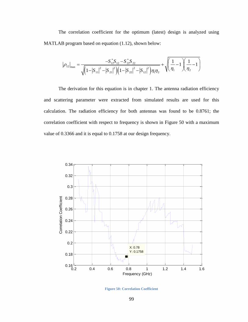
99
The correlation coefficient for the optimum (latest) design is analyzed using
MATLAB program based on equation (1.12), shown below:
* *
11 12 21 2212 max 2 2 2 2
1 211 21 22 12 1 2
1 11 1
1 1
S S S S
S S S S
The derivation for this equation is in chapter 1. The antenna radiation efficiency
and scattering parameter were extracted from simulated results are used for this
calculation. The radiation efficiency for both antennas was found to be 0.8761; the
correlation coefficient with respect to frequency is shown in Figure 50 with a maximum
value of 0.3366 and it is equal to 0.1758 at our design frequency.
Figure 50: Correlation Coefficient
0.2 0.4 0.6 0.8 1 1.2 1.4 1.60.16
0.18
0.2
0.22
0.24
0.26
0.28
0.3
0.32
0.34
X: 0.78
Y: 0.1758
Frequency (GHz)
Corr
ela
tion C
oeff
icie
nt
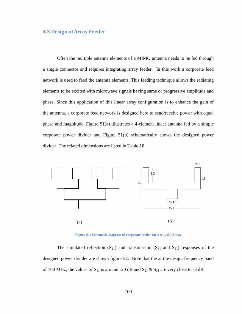
100
4.3 Design of Array Feeder
Often the multiple antenna elements of a MIMO antenna needs to be fed through
a single connector and requires integrating array feeder. In this work a corporate feed
network is used to feed the antenna elements. This feeding technique allows the radiating
elements to be excited with microwave signals having same or progressive amplitude and
phase. Since this application of this linear array configuration is to enhance the gain of
the antenna, a corporate feed network is designed here to send/receive power with equal
phase and magnitude. Figure 51(a) illustrates a 4-element linear antenna fed by a simple
corporate power divider and Figure 51(b) schematically shows the designed power
divider. The related dimensions are listed in Table 10.
Figure 51: Schematic diagram of corporate feeder (a) 4-way (b) 2-way
The simulated reflection (S11) and transmission (S31 and S21) responses of the
designed power divider are shown figure 52. Note that the at the design frequency band
of 700 MHz, the values of S11 is around -20 dB and S21 & S31 are very close to -3 dB.
(a) (b)

101
Table 10: Dimensions of the two way Power Divider of figure 4.5 (a)
W1 W2 W3 L1 L2 L3
5.36 mm 1.651 mm 21.651 mm 6 mm 4.349 mm 10 mm
Figure 52: S Parameters for the Two Port Power Divider
4.4 Design of a Two-Element MIMO Antenna Array
To reducing the multiple-access interference, MIMO antennas often employ
beam-forming technique. Using this technique the antenna gain can be increased in the
direction of the desired user, whilst reducing the gain towards the interfering users.
Although investigating this technique is not the objective of this research work, a simple
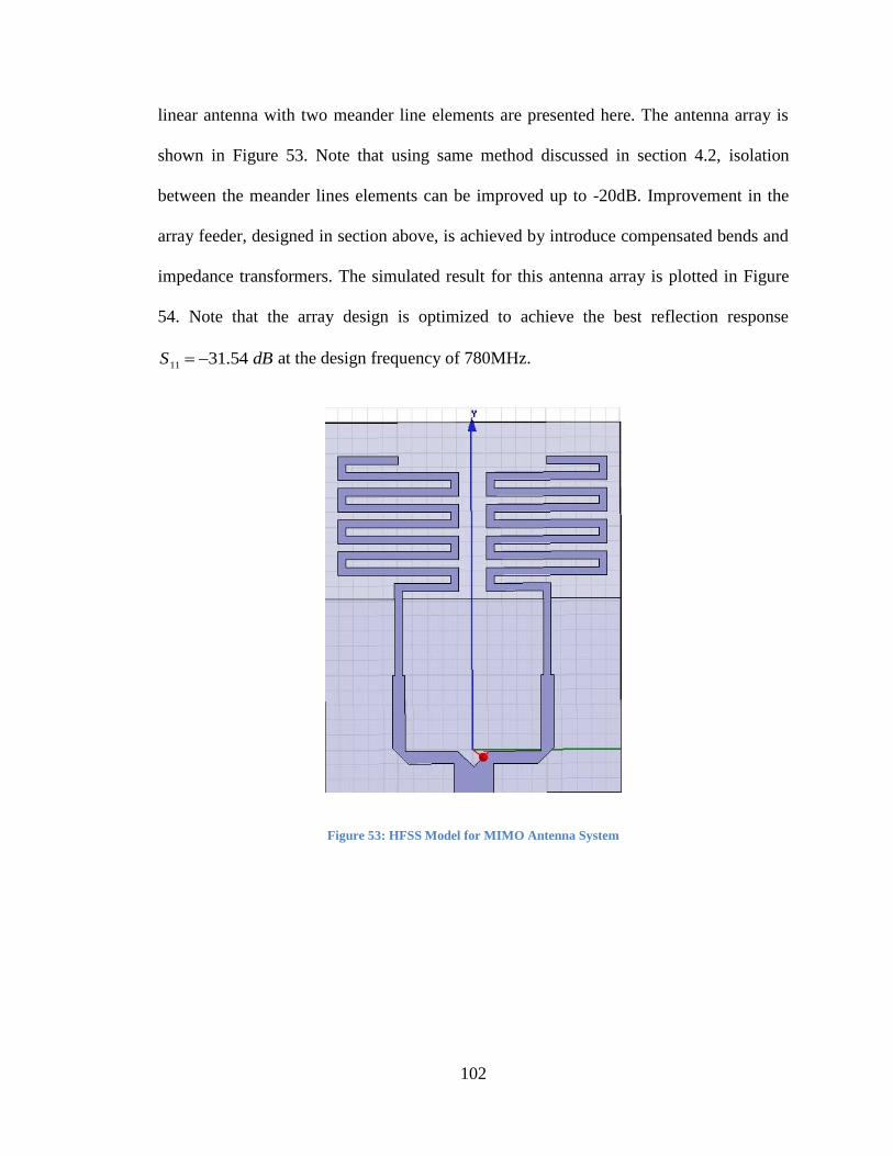
102
linear antenna with two meander line elements are presented here. The antenna array is
shown in Figure 53. Note that using same method discussed in section 4.2, isolation
between the meander lines elements can be improved up to -20dB. Improvement in the
array feeder, designed in section above, is achieved by introduce compensated bends and
impedance transformers. The simulated result for this antenna array is plotted in Figure
54. Note that the array design is optimized to achieve the best reflection response
11 31.54 S dB at the design frequency of 780MHz.
Figure 53: HFSS Model for MIMO Antenna System
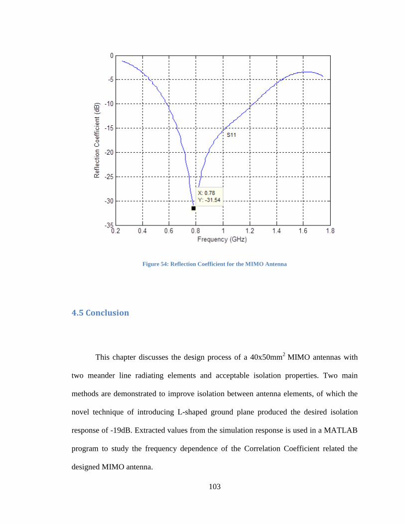
103
Figure 54: Reflection Coefficient for the MIMO Antenna
4.5 Conclusion
This chapter discusses the design process of a 40x50mm2
MIMO antennas with
two meander line radiating elements and acceptable isolation properties. Two main
methods are demonstrated to improve isolation between antenna elements, of which the
novel technique of introducing L-shaped ground plane produced the desired isolation
response of -19dB. Extracted values from the simulation response is used in a MATLAB
program to study the frequency dependence of the Correlation Coefficient related the
designed MIMO antenna.
104
CHAPTER 5
EXPERIMENTAL RESULTS
This chapter describes the fabrication and experimental results for the single and
dual element antenna for LTE handsets.
5.1 Experimental Setup
S-parameter measurements:
Since HP 8510 Vector Network Analyzer allows the measurement of reflection
and transmission relate S-parameter, it a very popular tool in measuring active and
passive microwave devices [74]. A network analyzer is used in this study to measure the
scattering parameters of the designed antennas.
Radiation measurements:
The radiation characteristics of the antennas were measured using the antenna
training and measurement system (ATMS) available at the KFUPM laboratory. Figure
55 shows the setup used for this purpose. The distance d was about 1.5 m.
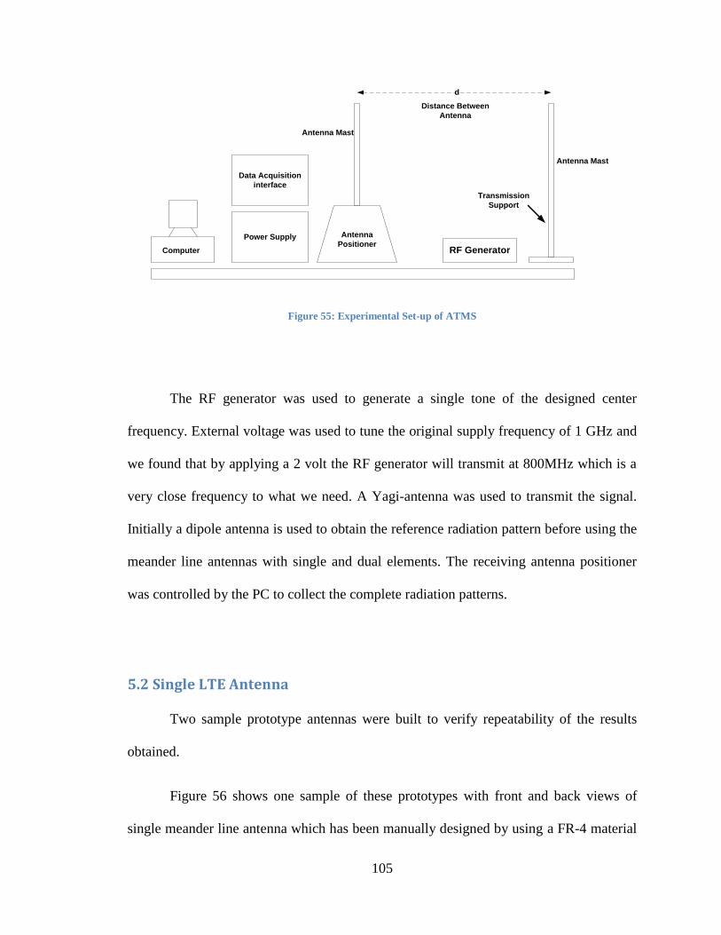
105
Data Acquisition
interface
Power Supply
RF GeneratorComputer
Antenna
Positioner
Antenna Mast
Antenna Mast
Transmission
Support
Distance Between
Antenna
d
Figure 55: Experimental Set-up of ATMS
The RF generator was used to generate a single tone of the designed center
frequency. External voltage was used to tune the original supply frequency of 1 GHz and
we found that by applying a 2 volt the RF generator will transmit at 800MHz which is a
very close frequency to what we need. A Yagi-antenna was used to transmit the signal.
Initially a dipole antenna is used to obtain the reference radiation pattern before using the
meander line antennas with single and dual elements. The receiving antenna positioner
was controlled by the PC to collect the complete radiation patterns.
5.2 Single LTE Antenna
Two sample prototype antennas were built to verify repeatability of the results
obtained.
Figure 56 shows one sample of these prototypes with front and back views of
single meander line antenna which has been manually designed by using a FR-4 material
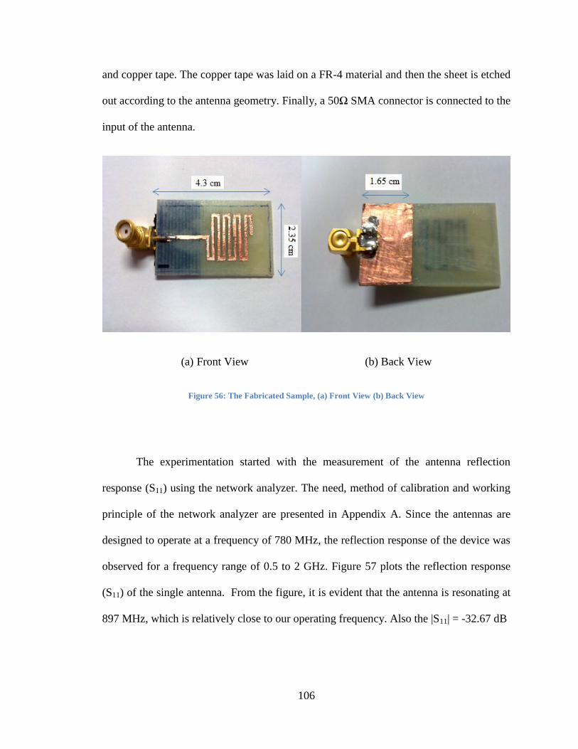
106
and copper tape. The copper tape was laid on a FR-4 material and then the sheet is etched
out according to the antenna geometry. Finally, a 50Ω SMA connector is connected to the
input of the antenna.
(a) Front View (b) Back View
Figure 56: The Fabricated Sample, (a) Front View (b) Back View
The experimentation started with the measurement of the antenna reflection
response (S11) using the network analyzer. The need, method of calibration and working
principle of the network analyzer are presented in Appendix A. Since the antennas are
designed to operate at a frequency of 780 MHz, the reflection response of the device was
observed for a frequency range of 0.5 to 2 GHz. Figure 57 plots the reflection response
(S11) of the single antenna. From the figure, it is evident that the antenna is resonating at
897 MHz, which is relatively close to our operating frequency. Also the |S11| = -32.67 dB

107
Figure 57: Experimental Reflection Coefficient for the Single Antenna
Figure 58 shows the reflection coefficient of the simulated and measured single
meander line antenna for an LTE handset. The behavior of both curves is in agreement. A
slight shift in the result frequency and measurement bandwidth was obtained from
measurement due to imperfect fabrication process. Table 11 summarizes the result of
Figure 58.
Table 11: Simulated and Experimental Results for Single MLA Antenna
Frequency Reflection Coefficient Bandwidth
Theoretical 780 MHz -30.9 260
Experimental 897.5 MHz -32.67 185.4
0.5 1 1.5 2-35
-30
-25
-20
-15
-10
-5
0
Frequency (GHz)
S p
ara
mete
rs
(d
B)
S11 for Single Antenna
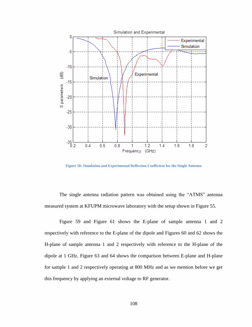
108
Figure 58: Simulation and Experimental Reflection Coefficient for the Single Antenna
The single antenna radiation pattern was obtained using the ―ATMS‖ antenna
measured system at KFUPM microwave laboratory with the setup shown in Figure 55.
Figure 59 and Figure 61 shows the E-plane of sample antenna 1 and 2
respectively with reference to the E-plane of the dipole and Figures 60 and 62 shows the
H-plane of sample antenna 1 and 2 respectively with reference to the H-plane of the
dipole at 1 GHz. Figure 63 and 64 shows the comparison between E-plane and H-plane
for sample 1 and 2 respectively operating at 800 MHz and as we mention before we get
this frequency by applying an external voltage to RF generator.
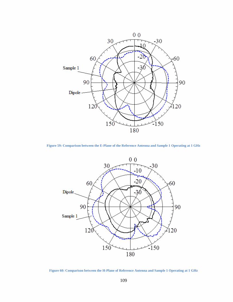
109
Figure 59: Comparison between the E-Plane of the Reference Antenna and Sample 1 Operating at 1 GHz
Figure 60: Comparison between the H-Plane of Reference Antenna and Sample 1 Operating at 1 GHz
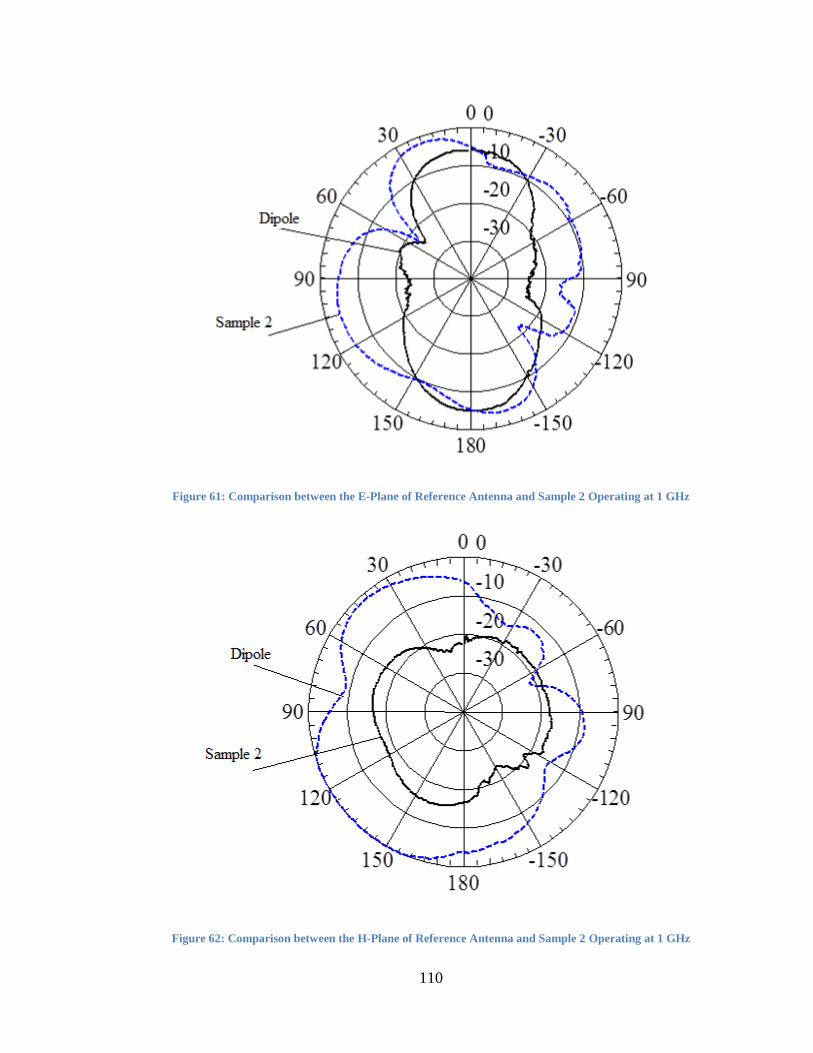
110
Figure 61: Comparison between the E-Plane of Reference Antenna and Sample 2 Operating at 1 GHz
Figure 62: Comparison between the H-Plane of Reference Antenna and Sample 2 Operating at 1 GHz
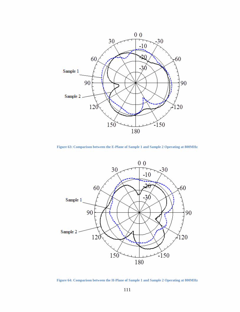
111
Figure 63: Comparison between the E-Plane of Sample 1 and Sample 2 Operating at 800MHz
Figure 64: Comparison between the H-Plane of Sample 1 and Sample 2 Operating at 800MHz
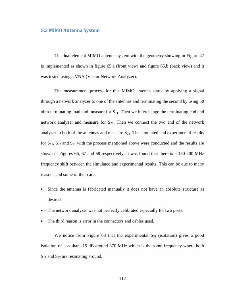
112
5.3 MIMO Antenna System
The dual element MIMO antenna system with the geometry showing in Figure 47
is implemented as shown in figure 65.a (front view) and figure 65.b (back view) and it
was tested using a VNA (Vector Network Analyzer).
The measurement process for this MIMO antenna starts by applying a signal
through a network analyzer to one of the antennas and terminating the second by using 50
ohm terminating load and measure for S11. Then we interchange the terminating end and
network analyzer and measure for S22. Then we connect the two end of the network
analyzer to both of the antennas and measure S21. The simulated and experimental results
for S11, S22 and S21 with the process mentioned above were conducted and the results are
shown in Figures 66, 67 and 68 respectively. It was found that there is a 150-200 MHz
frequency shift between the simulated and experimental results. This can be due to many
reasons and some of them are:
Since the antenna is fabricated manually it does not have an absolute structure as
desired.
The network analyzer was not perfectly calibrated especially for two ports.
The third reason is error in the connectors and cables used.
We notice from Figure 68 that the experimental S21 (isolation) gives a good
isolation of less than -15 dB around 870 MHz which is the same frequency where both
S11 and S22 are resonating around.
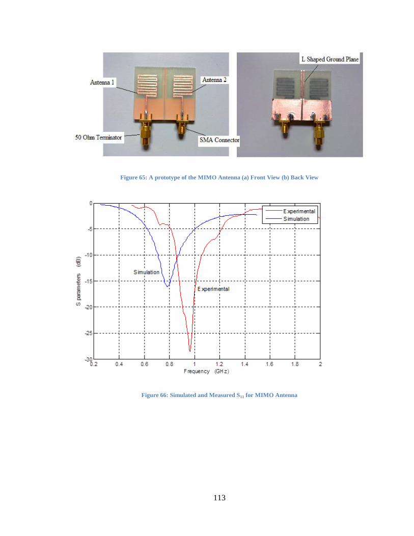
113
Figure 65: A prototype of the MIMO Antenna (a) Front View (b) Back View
Figure 66: Simulated and Measured S11 for MIMO Antenna
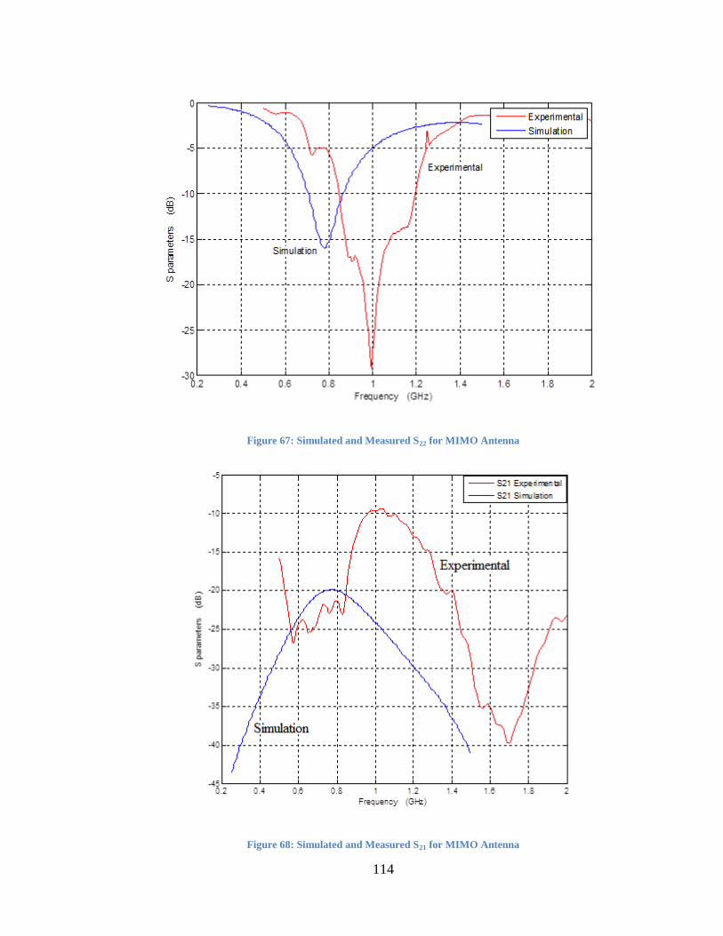
114
Figure 67: Simulated and Measured S22 for MIMO Antenna
Figure 68: Simulated and Measured S21 for MIMO Antenna
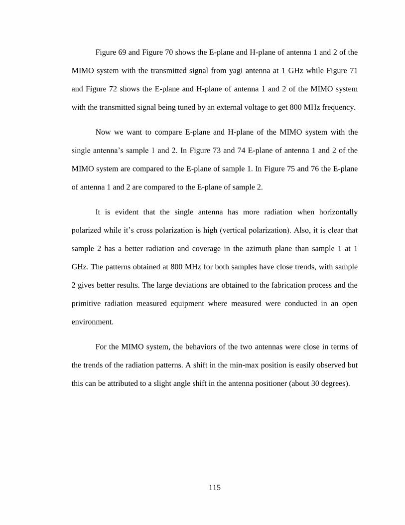
115
Figure 69 and Figure 70 shows the E-plane and H-plane of antenna 1 and 2 of the
MIMO system with the transmitted signal from yagi antenna at 1 GHz while Figure 71
and Figure 72 shows the E-plane and H-plane of antenna 1 and 2 of the MIMO system
with the transmitted signal being tuned by an external voltage to get 800 MHz frequency.
Now we want to compare E-plane and H-plane of the MIMO system with the
single antenna’s sample 1 and 2. In Figure 73 and 74 E-plane of antenna 1 and 2 of the
MIMO system are compared to the E-plane of sample 1. In Figure 75 and 76 the E-plane
of antenna 1 and 2 are compared to the E-plane of sample 2.
It is evident that the single antenna has more radiation when horizontally
polarized while it’s cross polarization is high (vertical polarization). Also, it is clear that
sample 2 has a better radiation and coverage in the azimuth plane than sample 1 at 1
GHz. The patterns obtained at 800 MHz for both samples have close trends, with sample
2 gives better results. The large deviations are obtained to the fabrication process and the
primitive radiation measured equipment where measured were conducted in an open
environment.
For the MIMO system, the behaviors of the two antennas were close in terms of
the trends of the radiation patterns. A shift in the min-max position is easily observed but
this can be attributed to a slight angle shift in the antenna positioner (about 30 degrees).
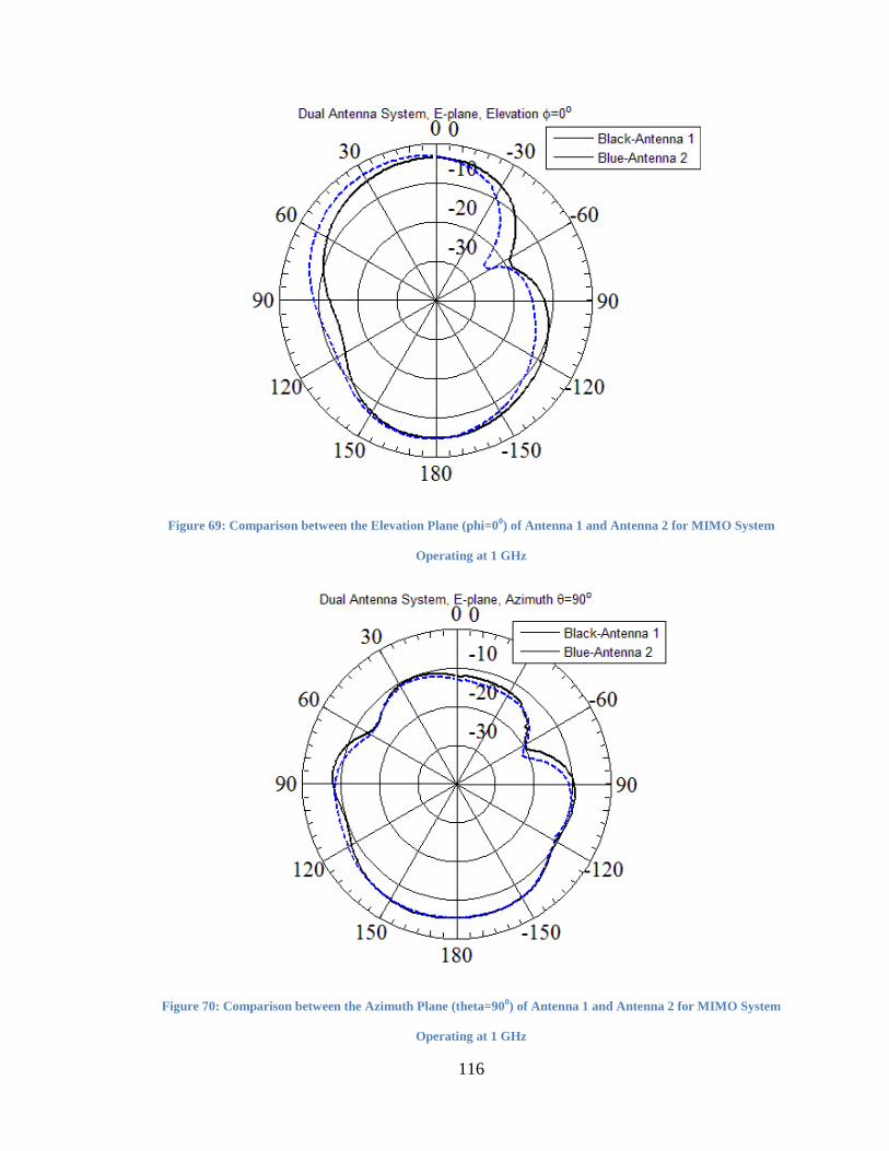
116
Figure 69: Comparison between the Elevation Plane (phi=00) of Antenna 1 and Antenna 2 for MIMO System
Operating at 1 GHz
Figure 70: Comparison between the Azimuth Plane (theta=900) of Antenna 1 and Antenna 2 for MIMO System
Operating at 1 GHz

117
Figure 71: Comparison between the E-Plane of Antenna 1 and Antenna 2 for MIMO System at 800MHz
Figure 72: Comparison between the H-Plane of Antenna 1 and Antenna 2 for MIMO System at 800MHz
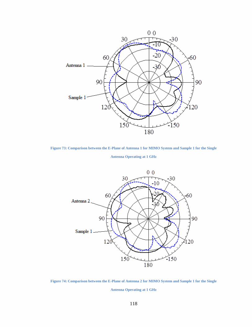
118
Figure 73: Comparison between the E-Plane of Antenna 1 for MIMO System and Sample 1 for the Single
Antenna Operating at 1 GHz
Figure 74: Comparison between the E-Plane of Antenna 2 for MIMO System and Sample 1 for the Single
Antenna Operating at 1 GHz
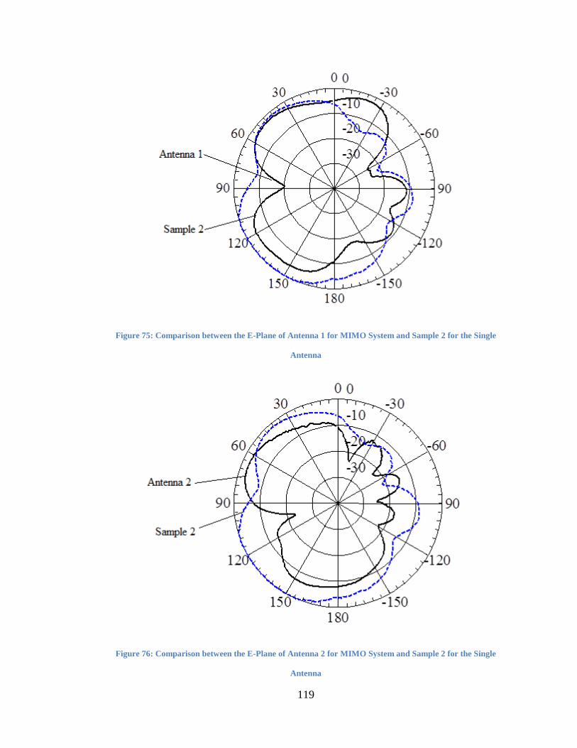
119
Figure 75: Comparison between the E-Plane of Antenna 1 for MIMO System and Sample 2 for the Single
Antenna
Figure 76: Comparison between the E-Plane of Antenna 2 for MIMO System and Sample 2 for the Single
Antenna

120
5.4 Conclusion
In this chapter we had an overview of the fabrication and experimental process for
both single element and MIMO antenna system. We have compared between simulated
and experimental results for each of these antennas and found that there are some
variations since we are dealing with antenna with many bends. The percentage of error in
the resonant frequency was 19.17% in the dual antenna and 13.09% in the single antenna.
Also, the radiation patterns were examined. A noticeable variation was observed between
the two samples, but general trends look alike. The antennas fabricated worked around 1
GHz.
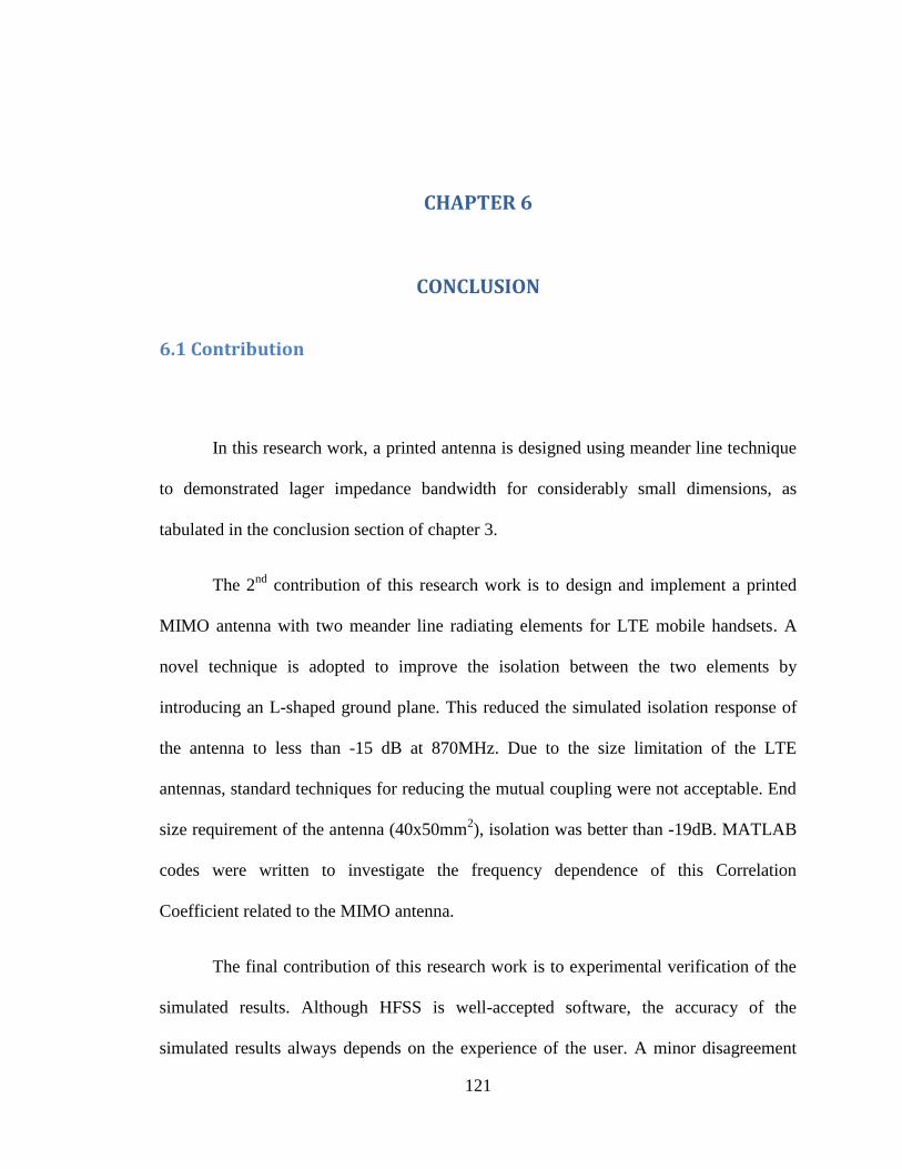
121
CHAPTER 6
CONCLUSION
6.1 Contribution
In this research work, a printed antenna is designed using meander line technique
to demonstrated lager impedance bandwidth for considerably small dimensions, as
tabulated in the conclusion section of chapter 3.
The 2nd
contribution of this research work is to design and implement a printed
MIMO antenna with two meander line radiating elements for LTE mobile handsets. A
novel technique is adopted to improve the isolation between the two elements by
introducing an L-shaped ground plane. This reduced the simulated isolation response of
the antenna to less than -15 dB at 870MHz. Due to the size limitation of the LTE
antennas, standard techniques for reducing the mutual coupling were not acceptable. End
size requirement of the antenna (40x50mm2), isolation was better than -19dB. MATLAB
codes were written to investigate the frequency dependence of this Correlation
Coefficient related to the MIMO antenna.
The final contribution of this research work is to experimental verification of the
simulated results. Although HFSS is well-accepted software, the accuracy of the
simulated results always depends on the experience of the user. A minor disagreement
122
between the simulated and experimental results (see conclusion of chapter 5) were due to
the inaccuracy of the in house fabrication process.
6.2 Future Work
Use Meta-material based substrates to further reduce the antenna size and
introduce external control.
Design and implement 4x4 MIMO antenna systems for LTE standards of mobile
phones with reduced correlation coefficient. This is particularly challenging due
to the size limitations and usage of 700 MHz band for this system.
123
Appendix A
Experimental Process
After we fabricate the antennas we need to test it in order to verify the simulation
results, we start by testing the operating frequency of the antenna and the reflection
coefficient and the bandwidth using network analyzer but before using it we need to
calibrate it and test that calibration in order to eliminate any errors my caused by
calibration, cables and connectors and the following topic is how to calibrate the network
analyzer.
Network Analyzer Calibration
1. Turn on the power. You will turn on four "Line/Power" buttons.
2. Attach connectors and extra cables to the network analyzer as needed. Be careful
with the network analyzer cables. Do not over bend them.
Calibrate the network analyzer (S11 or S22 Reflection Measurements only).
a. Choose a calibration kit for the type of connector you are using.
b. Set your frequency range. Press start and type the frequency you want to start. Do
the same for the stop frequency.
124
c. On the MENUS control, press CAL. Delete a calibration set to make empty slot
for yours. Do these by pressing MORE on the soft menu on the screen, then
DELETE CAL SET, then choose a number.
d. Select a calibration type. Generally this is the type of cable connected to the
network analyzer.
e. Choose S11-1 port or S22- 1 port (depending on which cable you want to use).
f. You will be prompted to put calibration standards on the end of your cable. They
are in the wooden box.
1. Start with the short (it is labeled). Connect the short, press the soft key
SHORT, and when it is done measuring (quickly) it will underline the
SHORT. Take it off, put the plastic cover back on the standard, and find
the open.
2. Open. It is the same length as the short, but with a smaller radius and a
hole in the end. Press OPEN, wait until open is underlined, remove the
open and replace the plastic cover.
3. Find the load standard. They are the long, sliding cylinders in the box.
Connect it, and press LOAD. Then BROADBAND. Then DONE LOADS.
We are assuming our load is accurate over the whole frequency range of
calibration and is therefore "broadband." Replace the plastic cover; put all
the standards back in the box.
a. Press SAVE 1-port CAL. Press the number where you want to save the calibration
settings. It should say "Correction ON"

125
b. Test your calibration. The worst is usually the open. Test the short and load the
same way. IF these are not "clean", redo the calibration. Factors that can affect
your calibration: tightness of cables and connectors, between elements and to the
network analyzer.
c. If your calibration is good. PUT THE BOX of standards back in the closet. [75]
After the calibration is ready we can now take the results.

126
Appendix B
Simulator Software Used
B.1 What is HFSS?
HFSS is a commercial finite element method solver for electromagnetic structures
from Ansoft Corporation. The acronym originally stood for high frequency structural
simulator. It is one of the most popular and powerful applications used for antenna design
and the design of complex RF electronic circuit elements including filters, transmission
lines, and packaging. It was originally developed by Professor Zoltan Cendes and his
students at Carnegie Mellon University. Prof. Cendes and his brother Nicholas Cendes
founded Ansoft and sold HFSS stand-alone under a 1989 marketing relationship with
Hewlett-Packard, and bundled into Ansoft products. [76]
The power of HFSS (Version 12 the one we have) software comes from many
research and development innovations, which have made i t the most widely used
software for solving 3-D full-wave electromagnetic field simulations. The invention of
tangential vector basis functions enabled the highly accurate finite element method for
electromagnetic field solution. The transfinite element method allowed the 3-D finite
element solution to couple to port solutions for fast and accurate multi-mode s-parameter
extractions. Finally, the development of automatic mesh generation and adaptive
refinement was a key innovation for reliable, repeatable and efficient results. [77]
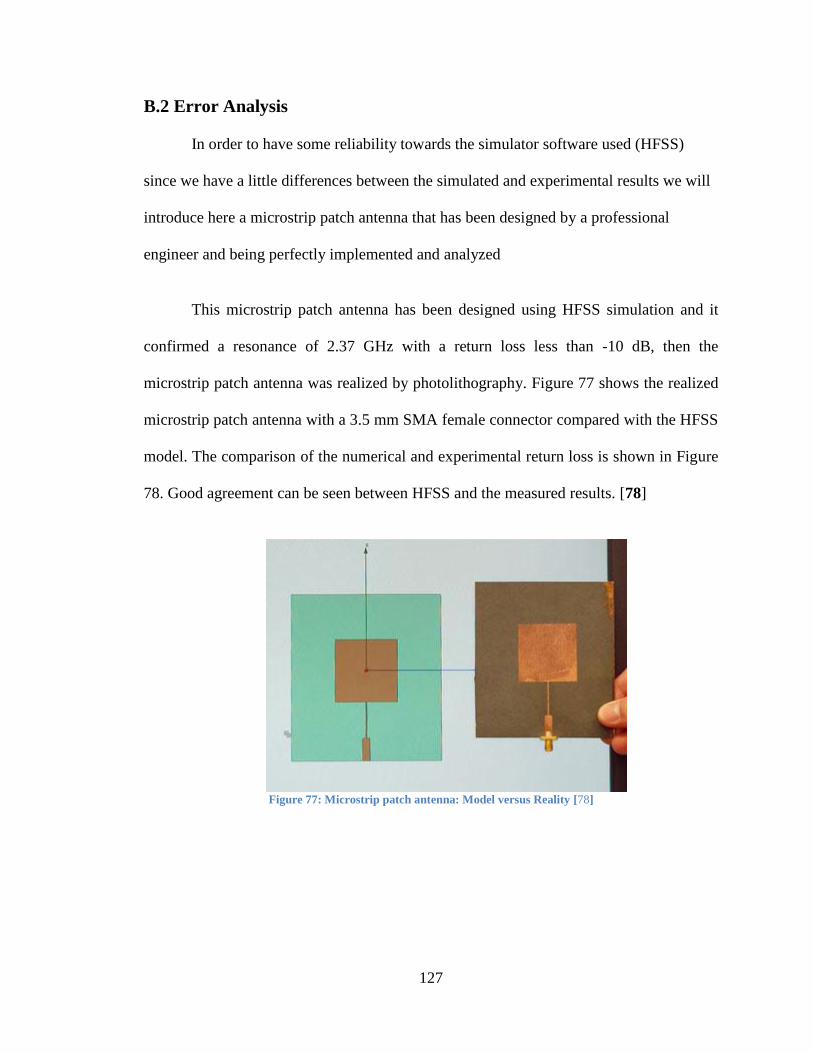
127
B.2 Error Analysis
In order to have some reliability towards the simulator software used (HFSS)
since we have a little differences between the simulated and experimental results we will
introduce here a microstrip patch antenna that has been designed by a professional
engineer and being perfectly implemented and analyzed
This microstrip patch antenna has been designed using HFSS simulation and it
confirmed a resonance of 2.37 GHz with a return loss less than -10 dB, then the
microstrip patch antenna was realized by photolithography. Figure 77 shows the realized
microstrip patch antenna with a 3.5 mm SMA female connector compared with the HFSS
model. The comparison of the numerical and experimental return loss is shown in Figure
78. Good agreement can be seen between HFSS and the measured results. [78]
Figure 77: Microstrip patch antenna: Model versus Reality [78]

128
Figure 78: Return loss of the microstrip patch antenna [78]
B.3 Ansoft HFSS Tutorial: Dipole Antenna
This tutorial introduces the interface of Ansoft’s HFSS, and walks the student
through an example problem of creating, simulating and evaluating the response of a
standard stripline structure. [79]
1. HFSS Interface
The main HFSS interface is shown in Figure 79, which illustrates the main
components of the GUI (Graphical User Interface). They are summarized as follows:
• 3D Modeler Window This is the area where you create the model geometry. This
window consists of the model view area (or grid) and the history tree as shown in Figure

129
80. The history tree documents the actions that have been taken in the model view area,
and provides an alternative way to select objects in the model view area.
• Project Manager with Project Tree The project manager window displays details
about all open HFSS projects. Each project ultimately includes a geometric model, its
boundary conditions and material assignments, and field solution and post processing
information. An expanded view of the project manager is shown in Figure 81.
• Properties Window The properties window consists of two tabs. The command tab
displays information about an action selected in the history tree that was performed to
either create an object or modify an object. The attribute tab displays information about
the material and display properties of a selected object.
• Progress Window This window is used when a simulation is running to monitor the
solution’s progress.
• Message Manager This window displays messages associated with a project’s
development (such as error messages about the design’s setup)
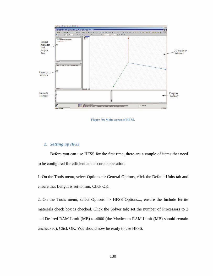
130
Figure 79: Main screen of HFSS.
2. Setting up HFSS
Before you can use HFSS for the first time, there are a couple of items that need
to be configured for efficient and accurate operation.
1. On the Tools menu, select Options => General Options, click the Default Units tab and
ensure that Length is set to mm. Click OK.
2. On the Tools menu, select Options => HFSS Options..., ensure the Include ferrite
materials check box is checked. Click the Solver tab; set the number of Processors to 2
and Desired RAM Limit (MB) to 4000 (the Maximum RAM Limit (MB) should remain
unchecked). Click OK. You should now be ready to use HFSS.

131
3. Example: Dipole Antenna
To begin to appreciate the functionality of this simulation tool, we will create and
simulate a simple loop antenna. Before we can begin to work through the simulation
though, we need to design the antenna on paper. This design will consist of a half-wave
dipole antenna with center frequency of 300MHz. At this frequency, the wavelength in
free-space is
8
6
3*101
300*10
cm
f
Figure 80: 3D Modeler Window, which consists of the model view area and the history tree
So, the total antenna length should be ℓ = λ/2 = 0.5 m. Now, the only items remaining are
the radius of the wires and the gap between the wires at the feed point. These items are
difficult to determine analytically, so we will simply define them to be (r = 0.1 mm), and
(g = 20 mm). With these choices, we expect to have an omnidirectional pattern in the far
field.

132
3.1 Creating the Antenna
Now it’s time to build this model in HFSS. We’ll begin with the radiating
structure itself. To do so, we’ll create a series of cylindrical shapes by selecting Draw =>
cylinder in the file menu. To make the cylinder the correct size, you can either
1. Input the x, y, z coordinates of the center point, radius and height of the cylinder into
the appropriate fields at the bottom of the 3D model window, or
2. Click randomly in the 3D model window three times to create a cylinder and edit the
size in the properties box. To do this, click the command tab in the properties box and
input the correct center point, radius and height for our cylinder.
For this design, we’ll choose the center point to be placed at the location 0,0,10
mm, the radius should equal 0.1mm and the height should be 240mm. Next, we’ll create
the other half of the radiating element. This will be another cylinder with center point at
0,0,-10 mm, radius 0.1mm and height of -0.240mm.
Next we need to create the feed structure. To do so, we need to create two more
cylinders, and two spheres. The cylinders will occur in the zx–plane, so we need to
change the desired plane accordingly in the pull-down menu. Then, we create two
cylinders,

133
Figure 81: Project Manager Window illustrating the boundary conditions, excitation, etc. of the current model
• The first with center at 0,0,10 mm, radius = 0.1mm, and height = 250mm
• The second with center at 0,0,-10 mm, radius = 0.1mm, and height = 250mm
Now, we have an incomplete connection between the feed wires and the radiating
wires. To complete this connection, we’ll add two spheres at the junction.
• The first with center at 0,0,10 mm, and radius = 0.1mm
• The second with center at 0,0,-10 mm, and radius = 0.1mm
Now select all items that you have drawn so far and select Modeler => Boolean => Unite.

134
Finally we will identify the resulting geometry as a perfect electric conductor (PEC) by
right clicking in the geometry window and selecting Assign Material. In the resulting
window, select PEC and click OK.
3.2 Creating the radiation box
Now, we need to establish a box around the antenna in which we will compute the
fields, and from which we will calculate the far-field response. To assure good far-field
calculations, the box should extend at least λ/4 away from all radiating surfaces. We will
choose the box to be centered on the antenna and λ/2 wide, so that all surfaces are at an
adequate distance from the antenna.
To draw the radiation box, select Draw => box and input the following parameters for the
box:
• Beginning point: -250mm, -250mm, -510mm
• The Cartesian sizes are: X size = 500mm, Y size = 500mm, and Z size = 1020mm
Now select the attribute tab and do the following:
• Ensure that the material is vacuum. If it is not, click the button next to material and
select vacuum as the material.
• Click the button next to transparent and set the transparency to 0.95.
Now, the model is complete.

135
3.3 Boundary Conditions
The following items need to be setup to assure a good simulation:
1. Mesh Operations: To ensure we receive a good quality far field calculation, we need
to ensure that the mesh is generated with sufficient accuracy on the outer boundary of the
domain. According to Ansoft, we can achieve sufficient accuracy if the following rules of
thumb are followed:
(a) The outer boundary must be at least λ/4 away from every radiating surface
(b) The mesh length must be constrained to be no greater than λ/6 on the boundary
The wavelength at 300 MHz in free space is λ = 1m, so the maximum length of elements
on the boundary is ℓmax = 0.16m.
To limit the mesh to this value, perform the following steps:
(a) Highlight the vacuum box
(b) Right click in the 3D modeler window and select Assign Mesh Operation => On
Selection => Length Based
(c) Set the maximum length of elements to 160mm
(d) Click OK
2. Radiation Boundary: To compute the radiated fields, we need to establish a radiation
boundary on all surfaces of the vacuum box. Do this, we right click in the drawing
window and click select faces. Then, click on each face of the vacuum box while holding

136
the control key. Once all faces are selected, right click again in the drawing window and
click assign boundary => Radiation.... Use all defaults on this boundary.
3. Far Field Calculation: To compute the radiated fields in the far-field, we need to tell
HFSS what level of granularity we want on the far-field sphere. To do so, right-click
radiation in the project tree and select Insert Far Field Setup => infinite sphere; use the
defaults for this sphere.
3.4 Excitations
We will create a ―WavePort‖ excitation at the feed lines of the antenna. To do so,
we perform the following steps:
1. Create a rectangle in the zx-plane with first point (-25mm, 250mm, -24.85mm) and
axis = Y, X size = 50mm, Z size = 50mm
2. Select the resulting rectangle
3. Right-click in the 3D modeler window and select Assign Excitation => Wave Port.
4. Click Next
5. Under ―Integration Line,‖ click the word None, and select New Line...
6. In the 3D modeler window, click the center of the bottom wire
7. Click the center of the top wire
8. Click Next
9. Click Finish

137
3.5 Analysis
Perform the following steps to set up the analysis options:
1. Right click on Analysis in the Project Tree, and select ―Add Solution Setup‖
2. Under the General tab:
(a) Set the solution frequency to 300 MHz
(b) Set the maximum number of passes to 30
(c) Set maximum Delta S to 0.01
3. Under the Options tab:
(a) Set the Maximum Refinement per pass to 20 %
(b) Set the Order of Basis Functions to First Order
4. Under the Advanced Tab, check the box titled Use Radiation Boundary on Ports
5. Click OK
Perform the following steps to set up a frequency sweep (if desired):
1. Under the Analysis item in the Project Tree, right-click on Setup1
2. Select Add Frequency Sweep...3. Set start frequency to 20 MHz
4. Set stop frequency to 300 MHz
5. Set step size to 20 MHz

138
6. Click OK
3.6 Final Checks and Running the Simulation
Select HFSS => Validation Check... to ensure the project is prepared for simulation (click
close).
Save the project by clicking on the save icon at the top of the screen. Right-click
setup1 under Analysis in the project tree, select Analyze to begin the simulation. At this
point the progress window should show the progress of the simulation, beginning with
the mesh generation.
3.7 Simulation Results
To view the far-field results of the simulation, perform the following steps:
1. Right click on the results item in the Project Tree
2. Click Create Far-Fields Report => 3D Polar Plot
3. Under the trace tab, select Gain
4. Add trace by clicking the Add Trace button
5. Click Close
To view the impedance results of the simulation, perform the following steps:
1. Right click on the results item in the Project Tree
2. Click Create Modal Solution Data Report => Rectangular Plot

139
3. Under the trace tab, select Z-Parameter, Z(1,1), highlight re and im with the control
key
4. Add traces by clicking the Add Trace button
5. Click Close

140
Bibliography
[1] Kevin Peter. Analysis and Comparison of 1G , 2G , 3G ,4G and 5G Telecom
Services. [Online]. http://hubpages.com/hub/3G-and-4G-Mobile-Services
[2] ITU. (2002) Mobile cellular, subscribers per 100 people. [Online].
http://www.itu.int/ITU-D/ict/statistics/at_glance/cellular02.pdf
[3] Y., Jeong, B.J., Chung, J., Hwang, C., Ryu, J.S., Kim, K., Kim, Y.K. Kim, "Beyond
3G: Vision, Requirements, and Enabling Technologies," pp. 120-124, March 2003.
[4] 2G – 3G Cellular Wireless data transport terminology. [Online].
www.arcelect.com/2G-3G_Cellular_Wireless.htm
[5] Mohammad S. Sharawi, "RF Planning and Optimization for LTE Networks," in
Evolved Cellular Network Planning and Optimization for UMTS and LTE, Lingyang
Song Jia Shen, Ed.: CRC Press, To appear 2010, ch. 11, pp. 399-432.
[6] Vasco Pereira and Tiago Sousa, "Evolution of Mobile Communications: from 1G to
4G," Department of Informatics Engineering of the University of Coimbra,.
[7] Christian Papassarandis, "Introduction to LTE," in LTE Workshop, KFUPM,
Dhahran, 2010.
[8] NOKIA. LTE - Delivering the optimal upgrade path for 3G networks. [Online].
http://www.nokia.com/NOKIA_COM_1/Press/Press_Events/Nokia_Technology_M
edia_Briefing/LTE_Press_Backgrounder.pdf

141
[9] Motorola. TECHNICAL WHITE PAPER: Long Term Evolution (LTE): A
Technical Overview. [Online]. www.motorola.com/lte
[10] J. B. Andersen, J. P. Kermoal and P. Mogensen K. I. Pedersen, "A Stochastic
Multiple-Input-Multiple-Output Radio Channel Model for Evaluation of Space-
Time Coding Algorithms," Proceedings of IEEE Vehicular Technology Conference,
pp. 893-897, 2000.
[11] Ko S. C. K. and Murch D., "Compact Integrated Diversity Antenna for Wireless
Communications," IEEE Transaction on Antennas and Propagation Letters, vol. 9,
pp. 954-960, June 2001.
[12] Paul Hallbjörner, "Antennas, The Significance of Radiation Efficiencies When
Using S-Parameters to Calculate the Received Signal Correlation From Two," IEEE
ANTENNAS AND WIRELESS PROPAGATION LETTERS, vol. 4, pp. 97-99, 2005.
[13] Salonen I. and Vainikainen P., "Estimation of Signal Correlation in Antenna
Arrays," Proc. JINA Int. Symp. Antennas, vol. 2, pp. 383-386, Nov 2002.
[14] J. Romeu, and I. Corbella S. Blanch, "Exact representation of antenna system
diversity performance from input parameter description," IEE Electron. Lett, vol. 39,
no. 9, pp. 705–707, May 1 2003.
[15] V. Plicanic, T. Bolin, G. Kristensson, and A. Derneryd Z. Ying, "Characterization of
multi-channel antenna performance for mobile terminal by using near field and far
field parameters," presented at the COST 273 TD(04)(095), June 7–9 2004.

142
[16] D. M. Pozar, "Microwave Engineering," Addison Wesley, pp. 220-226, 1990.
[17] D. M. Pozar, "Microwave Engineering," Addison Wesley, pp. 228-230, 1990.
[18] Wikipedia. [Online].
http://en.wikipedia.org/wiki/700_MHz_wireless_spectrum_auction
[19] Constantine A Balanis, Antenna theory-Analysis and Design, 2nd ed.: John Wiley &
Sons Ltd, 1997.
[20] S Taylor., J Simkin, J M Oakley., C Emson and M J Lancaster H Y Wang,
"SIMULATION OF MICROSTRIP SMALL ANTENNAS ," Vector Fields Limited.
[21] Alok Singh, Amit Kumar Singh, Sandeep Kumar, Triloki Kumar O P N Calla,
"Empirical Relation for Designing the Meander Line Antenna," in International
Centre for Radio Science, Jodhpur-342003, Shobhit Institute of Engg & Technology,
Meerut, 2008.
[22] I. A. Salamat, M. F. Abdul Kadir, M. R. Che Rose, M. S. R. Mohd Shah, D.
Misman, "The Effect of Conductor Line to Meander Line Antenna Design," in
ASIA-Pacific Conference on Applied Electromagnetic Proceedings, 2007.
[23] Randy Bancroft, "Fundamental Dimension Limits of Antennas," Westminster,
Colorado, White paper, Centurion Wireless Technologies.
[24] Hing Kiu Kan and Rod B. Waterhouse, "Shorted Spiral-Like Printed Antennas,"
IEEE TRANSACTIONS ON ANTENNAS AND PROPAGATION, vol. 50, no. 3,

143
March 2002.
[25] Rod B. Waterhouse, "Small microstrip patch antenna," Electron. Lett., vol. 31, pp.
604-605, April 1995.
[26] Y. Hwang, E. K. W. Lam, and B. Lee T. K. Lo, "Miniature aperture coupled
microstrip antenna of very high permittivity," Electron. Lett., vol. 33, pp. 9-10, Jan
1997.
[27] K.-L. Wong and Y. F. Lin, "Small broadband rectangular microstrip antenna with
chip-resistor loading," Electron. Lett., vol. 33, pp. 1593–1594, Sept 1997.
[28] H. K. Kan and R. B. Waterhouse, "Size reduction technique for shorted patches,"
Electron. Lett., vol. 35, pp. 948–949, June 1999.
[29] D. J. Kim and Y. M. Moon K. S. Min, "Improved MIMO Antenna by Mutual
Coupling Suppression between Elements," Proceedings of the IEEE European
Conference on Wireless Technology, pp. 125-128, 2005.
[30] K. L. Wong, Planar Antennas for Wireless Communications.: Wiley, 2003.
[31] P. S. Hall, and D. Wake Z. D. Liu, "Dual-frequency planar inverted F antenna,"
IEEE Trans. Antennas Propagat, vol. 45, pp. 1451-1458, Oct 1997.
[32] C. R. Rowell and R. D. Murch, "A compact PIFA suitable for dual-frequency
900/1800-MHz operation," IEEE Trans. Antennas Propagation, vol. 46, pp. 596-
598, April 1998.

144
[33] F. R. Hsiao and K. L. Wong, "A shorted patch antenna with an L-shaped ground
plane for internal mobile handset antenna," Microwave Opt. Technol. Lett., vol. 33,
pp. 314-316, May 2002.
[34] Ansoft Corporation, "HFSS Online Help," V. 9.2,.
[35] Freescale Semiconductor. (2006, July) Compact Integrated Antennas Application
Note.
[36] R., Bhartia, P., Bahl, I. Garg, Microstrip Antenna Design Handbook.: Artech House,
Inc, 2001.
[37] G., and Ray, K.P. Kumar, Broadband Microstrip Antennas.: Artech House, Inc,
2003.
[38] B. R. Waterhouse, Microstrip Patch Antennas: A Designer’s Guide.: Kluwer
Academic Publishers, 2003.
[39] P. S. Nakar, Design of a compact Microstrip Patch Antenna for use in
Wireless/Cellular Devices.: Masters Thesis report, 2004.
[40] Frank M. Caimi. (2002) SkyCross, Inc.
[41] Z. Du, Q. Wang and K. Gong F. Wang, "Enhanced-bandwidth PIFA with T-shaped
ground plane," Electronic Letters, vol. 40, no. 23, pp. 1504 – 1505, Nov 2004.
[42] J. Hoon and H. Choi B. Kim, "Small wideband PIFA for mobile phones at 1800

145
MHz," , vol. 1, May 2004, pp. 27-29.
[43] H.A. Wheeler, "Fundamental Limits of Small Antennas," Proceedings of The I.R.E.
(IEEE), pp. 1479-1484, Dec. 1947.
[44] L. J. Chu, "Physical Limitations of Omni-Directional Antennas," Journal of Applied
Physics, vol. 19, pp. 1163-1175, Dec. 1948.
[45] R.C. Hansen, "Fundamental Limitations in Antennas," Proceedings of the IEEE, vol.
69, no. 2, pp. 170-182, Feb 1982.
[46] A. Henderson, K. Hirasawa and J.R. James K. Fujimoto, Small Antennas.: John
Wiley & Sons Inc., 1987.
[47] J. McLean, "A Re-Examination of the Fundamental Limits on the Radiation Q of
Electrically Small Antennas," IEEE Transactions on Antennas and Propagation,
vol. 44, no. 5, pp. 672-675, May 1996.
[48] H. Wheeler, "Small Antennas," in Antenna Engineering Handbook, R. Johnson, Ed.,
1993, ch. 6.
[49] Sumeet Sandhu. [Online]. http://www.comsoc.org/oeb/Past Presentations/Sumeet
June04.pdf
[50] I. E. Telatar, "Capacity of Multi-Antenna Gaussian Channels," European
Transactions on Telecommunications, vol. 10, pp. 585–595, 1999.

146
[51] S. Al-Ghadhban, "Multi-Layered Space Frequency Time Codes," Virginia
Polytechnic Institute and State University, Virginia, USA, PhD thesis Nov. 2005.
[52] J. Salz, "Digital transmission over cross-coupled linear channels," At&T Technical
Journal, vol. 64, no. 6, pp. 1147-1159, July-August 1985.
[53] O. Alamri,M. El-Hajjar, andN.Wu L.Hanzo, Near-CapacityMulti-Functional MIMO
Systems. UK: Wiley Press, 2009.
[54] "Applications of Antenna Arrays to Mobile Communications Part I: Performance
Improvement, Feasibility, and System Considerations," Proceedings of the IEEE,
vol. 85, pp. 1029–1030, July 1997.
[55] L. Godara, "Application of Antenna Arrays toMobile Communications. Part II.
Beam-Forming and Direction-of-Arrival Considerations," Proceedings of the IEEE,
vol. 85, pp. 1195–1245, Aug 1997.
[56] Christian Wolff. Phased Array Antenna. [Online].
http://www.radartutorial.eu/06.antennas/an14.en.html#this
[57] J. Litva and T. K. Lo, Digital Beamforming in Wireless Communications. Boston,
London: Artech House Publishers, 1996.
[58] T. Haynes, "A Primer on Digital Beamforming," Spectrum Signal Processing,
March 1998.
[59] T. H. Ismail and M. M. Dawoud, "Null Steering in Phased Arrays by Controlling the

147
Element Positions," lEEE Transactions on Antenna and Propagation, vol. AP-39,
no. 11, pp. 1561-1566, Nov 1991.
[60] M. M. Dawoud T. H. Ismail, ""Experimental Verificatoin of Null Steering by
Element Position Perturbations," IEEE Transactions on Antennas and Propagation,
vol. AP40, no. 11, pp. 1431-1434, Nov 1992.
[61] M. M. Dawoud, A. P. Anderson A. Tennant, "Array Pattem Nulling by Element
Position Perturbation using a Genetic Algorithm," Electronic Letters, vol. 30, no. 3,
pp. 174-176, February 1994.
[62] M. M. Dawoud, "Null Steering in Scanned Linear Arrays by Element Position
Perturbations," International Journal of Electronics, vol. 78, no. 4, pp. 743-757,
1995.
[63] M. J. Mismar and T. H. Ismail, "Null Steering using Minimax Approximation by
controlling only the Current Amplitudes," International Journal of Electronics, vol.
78, no. 2, pp. 409-415, February 1995.
[64] W. P. Liao and F. L. Chu, "Null Steering in Planar Arrays by controliing only
Current Amplitudes using Genetic Algorithms," Microwave and Optical Technology
Letters, pp. 97-103, 1997.
[65] W. P. Liao and F. L. Chu, "Application of Genetic Algorithms to Phase only Null
Steering of Linear Arrays," Electromagnetics, pp. 171-183, 1997.

148
[66] T. H. lsmail and M. J. Mismer, "Null Steering with Arbitmy Phase Perturbations
using Dual Phase Shiffers," Journal of EIectromagnetic Woes and Applications, vol.
13, no. 8, pp. 1021-1029, 1999.
[67] H. Steyskal, "Simple Method for Pattern Nulling by Phase Perturbations," IEEE
Transactions on Antennas and Propagation, vol. AP-31, pp. 163-166, January 1983.
[68] L. Zheng and D. N. C. Tse., "Diversity and multiplexing: A fundamental tradeoff in
multiple antenna channels," IEEE Transactions on Information Theory, vol. 49, pp.
1073–1096, May 2003.
[69] V. Erceg, D. Gesbert, and R. W. Heath Jr. S. Catreux, "Adaptive modulation and
MIMO coding for broadband wireless data networks," IEEE Communications
Magazine, vol. 40, no. 6, pp. 108-115, June 2002.
[70] V.V. Swarte,. Dehli: New Age International Limited, 1993, Reprint-2006, pp. 396,
397.
[71] Arto Hujanen, and Paivi K. Koivisto Johan C.—E. Sten, "Quality Factor of an
Electrically Small Antenna Radiating Close to a Conducting Plane," IEEE
Transactions on Antennas and Propagation, vol. 49, no. 5, p. 829—837, May 2001.
[72] Roger F. Harrington, "Effect of Antenna Size on Gain, Bandwidth, and Efficiency,"
Journal of Research of the National Bureau of Standards—D, Radio Propagation,
vol. 64D, no. 1, p. 1—12, January-February 1960.

149
[73] TACONIC. FR4 Processing Guide, Synthane-Taylor Laminates.
[74] N. Hercovici, "CAD of aperture coupled microstrip transmission lines and antennas:
software and user’s manual," Artech House, 1996.
[75] COE Department in UTAH University. Calibration and S-parameter Measurements
with the Network Analyzer. [Online].
http://www.coe.utah.edu/~cfurse/Tutorials/hp8510c/network%20analyzer.html
[76] Q&A With Zoltan Cendes, Founder, Chairman, And CTO Of Ansoft Corporation,
By Jim Pomager, Editor in Chief, RF Global Net.
[77] Director, Ansoft Product Management, ANSYS, Inc. By Larry Williams. (2009)
ANSYS Advantage. [Online]. http://www.ansys.com/magazine/issues/vol4-iss1-
2010/hfss.pdf
[78] EM Talk. [Online]. http://www.emtalk.com/mwt_mpa.htm
[79] Dr. Ryan S. Adams. (2009, September 8) Ansoft HFSS Tutorial: Dipole Antenna.

150
Vitae
NAME: Yanal Shaher Al-Faouri
BIRTH: 13th
July, Amman, JORDAN
EDUCATION: BACHELOR OF ENGINEERING (BSc)
Electrical Engineering,
University of Jordan,
Amman, JORDAN.
MASTER OF SCIENCE IN ELECTRICAL ENGINEERING
Department of Electrical Engineering
King Fahd University of Petroleum & Minerals
Dhahran, K.S.A.
CONTACT: [email protected]