deep learning early work why deep learning stacked auto encoders deep belief networks cs 678 –...
Post on 19-Dec-2015
241 views
TRANSCRIPT
Deep Learning
Early Work Why Deep Learning Stacked Auto Encoders Deep Belief Networks
CS 678 ndash Deep Learning 1
Deep Learning Overview
Train networks with many layers (vs shallow nets with just a couple of layers)
Multiple layers work to build an improved feature spacendash First layer learns 1st order features (eg edgeshellip)ndash 2nd layer learns higher order features (combinations of first layer
features combinations of edges etc)ndash In current models layers often learn in an unsupervised mode and
discover general features of the input space ndash serving multiple tasks related to the unsupervised instances (image recognition etc)
ndash Then final layer features are fed into supervised layer(s) And entire network is often subsequently tuned using supervised
training of the entire net using the initial weightings learned in the unsupervised phase
ndash Could also do fully supervised versions etc (early BP attempts)
CS 678 ndash Deep Learning 2
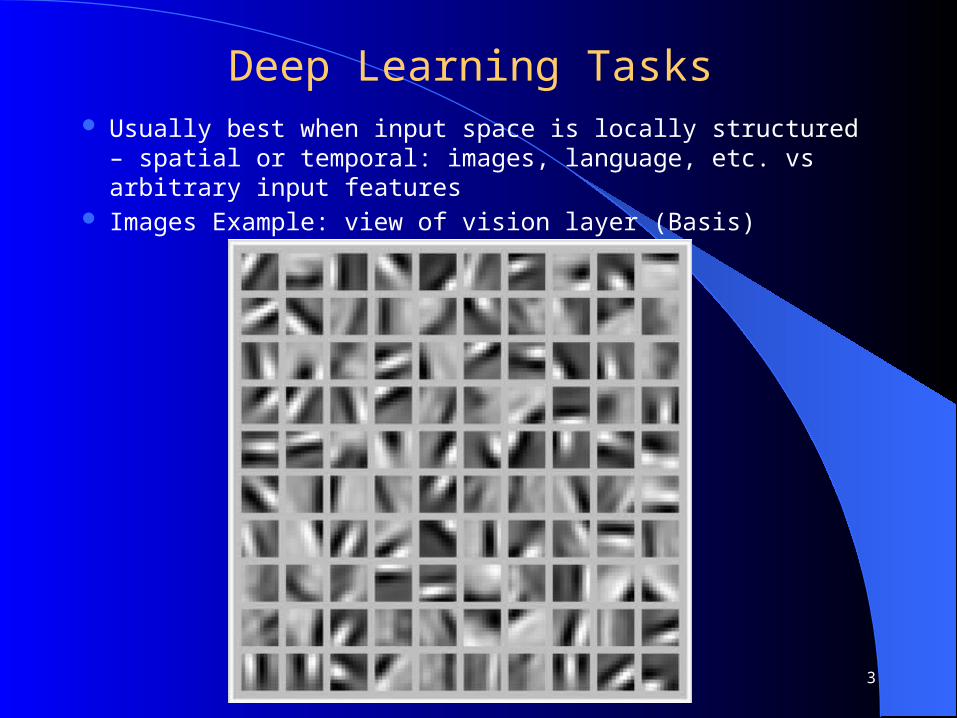
Deep Learning Tasks Usually best when input space is locally structured ndash spatial
or temporal images language etc vs arbitrary input features Images Example view of vision layer (Basis)
CS 678 ndash Deep Learning 3
Why Deep Learning
Biological Plausibility ndash eg Visual Cortex Hastad proof - Problems which can be represented with a
polynomial number of nodes with k layers may require an exponential number of nodes with k-1 layers (eg parity)
Highly varying functions can be efficiently represented with deep architecturesndash Less weightsparameters to update than a less efficient shallow
representation
Sub-features created in deep architecture can potentially be shared between multiple tasksndash Type of TransferMulti-task learning
CS 678 ndash Deep Learning 4
Early Work
Fukushima (1980) ndash Neo-Cognitron LeCun (1998) ndash Convolutional Neural Networks
ndash Similarities to Neo-Cognitron
Many layered MLP with backpropagationndash Tried early but without much success
Very slow Diffusion of gradient
ndash Very recent work has shown significant accuracy improvements by patiently training deeper MLPs with BP using fast machines (GPUs)
ndash We will focus on deep networks with unsupervised early layers
CS 678 ndash Deep Learning 5
Adobe ndash Deep Learning and Active Learning 6
BP Training Problems
hellip
bull Error attenuation long fruitless trainingbull Recent ndash Long patient training with GPUs and special hardwarebull However usually too time intensive for large networks
Convolutional Neural Networks Convolution Example Each layer combines (merges smoothes) patches from previous layers
ndash Typically tries to compress large data (images) into a smaller set of robust features based on local variations
ndash Basic convolution can still create many features Pooling ndash Pooling Example
ndash This step compresses and smoothes the datandash Make data invariant to small translational changesndash Usually takes the average or max value across disjoint patches
Often convolution filters and pooling are hand crafted ndash not learned though tuning can occur
After this hand-craftednon-trainedpartial-trained convolving the new set of features are used to train a supervised model
Requires neighborhood regularities in the input space (eg images stationary property)ndash Natural images have the property of being stationary meaning that the statistics of
one part of the image are the same as any other partCS 678 ndash Deep Learning 7
Convolutional Neural Network Examples
8
C layers are convolutions S layers poolsample
Training Deep Networks
Build a feature spacendash Note that this is what we do with SVM kernels or trained hidden
layers in BP etc but now we will build the feature space using deep architectures
ndash Unsupervised training between layers can decompose the problem into distributed sub-problems (with higher levels of abstraction) to be further decomposed at subsequent layers
CS 678 ndash Deep Learning 9
Training Deep Networks
Difficulties of supervised training of deep networksndash Early layers of MLP do not get trained well
Diffusion of Gradient ndash error attenuates as it propagates to earlier layers Leads to very slow training Exacerbated since top couple layers can usually learn any task pretty
well and thus the error to earlier layers drops quickly as the top layers mostly solve the taskndash lower layers never get the opportunity to use their capacity to improve results they just do a random feature map
Need a way for early layers to do effective workndash Often not enough labeled data available while there may be lots of
unlabeled data Can we use unsupervisedsemi-supervised approaches to take advantage
of the unlabeled datandash Deep networks tend to have more local minima problems than
shallow networks during supervised training
CS 678 ndash Deep Learning 10
Greedy Layer-Wise Training
One answer is greedy layer-wise training
1 Train first layer using your data without the labels (unsupervised)ndash Since there are no targets at this level labels dont help Could also use the
more abundant unlabeled data which is not part of the training set (ie self-taught learning)
2 Then freeze the first layer parameters and start training the second layer using the output of the first layer as the unsupervised input to the second layer
3 Repeat this for as many layers as desiredndash This builds our set of robust features
4 Use the outputs of the final layer as inputs to a supervised layermodel and train the last supervised layer(s) (leave early weights frozen)
5 Unfreeze all weights and fine tune the full network by training with a supervised approach given the pre-processed weight settings
CS 678 ndash Deep Learning 11
Deep Net with Greedy Layer Wise Training
Adobe ndash Deep Learning and Active Learning 12
ML Model
New Feature Space
Original Inputs
SupervisedLearning
UnsupervisedLearning
Greedy Layer-Wise Training
Greedy layer-wise training avoids many of the problems of trying to train a deep net in a supervised fashionndash Each layer gets full learning focus in its turn since it is the only
current top layerndash Can take advantage of unlabeled datandash When you finally tune the entire network with supervised training
the network weights have already been adjusted so that you are in a good error basin and just need fine tuning This helps with problems of
Ineffective early layer learning Deep network local minima
We will discuss the two most common approachesndash Stacked Auto-Encodersndash Deep Belief Networks
CS 678 ndash Deep Learning 13
Self Taught vs Unsupervised Learning
When using Unsupervised Learning as a pre-processor to supervised learning you are typically given examples from the same distribution as the later supervised instances will come fromndash Assume the distribution comes from a set containing just examples from a
defined set up possible output classes but the label is not available (eg images of car vs trains vs motorcycles)
In Self-Taught Learning we do not require that the later supervised instances come from the same distributionndash eg Do self-taught learning with any images even though later you will do
supervised learning with just cars trains and motorcyclesndash These types of distributions are more readily available than ones which just have
the classes of interestndash However if distributions are very differenthellip
New tasks share conceptsfeatures from existing data and statistical regularities in the input distribution that many tasks can benefit fromndash Note similarities to supervised multi-task and transfer learning
Both approaches reasonable in deep learning modelsCS 678 ndash Deep Learning 14
Auto-Encoders A type of unsupervised learning which tries to discover generic
features of the datandash Learn identity function by learning important sub-features (not by just passing
through data)ndash Compression etcndash Can use just new features in the new training set or concatenate both
15
Stacked Auto-Encoders Bengio (2007) ndash After Deep Belief Networks (2006) Stack many (sparse) auto-encoders in succession and train them using
greedy layer-wise training Drop the decode output layer each time
CS 678 ndash Deep Learning 16
Stacked Auto-Encoders Do supervised training on the last layer using final features Then do supervised training on the entire network to fine-
tune all weights
17
Sparse Encoders Auto encoders will often do a dimensionality reduction
ndash PCA-like or non-linear dimensionality reduction This leads to a dense representation which is nice in terms of
parsimonyndash All features typically have non-zero values for any input and the
combination of values contains the compressed information However this distributed and entangled representation can often
make it more difficult for successive layers to pick out the salient features
A sparse representation uses more features where at any given time a significant number of the features will have a 0 valuendash This leads to more localist variable length encodings where a particular
node (or small group of nodes) with value 1 signifies the presence of a feature (small set of bases)
ndash A type of simplicity bottleneck (regularizer)ndash This is easier for subsequent layers to use for learning
CS 678 ndash Deep Learning 18
How do we implement a sparse Auto-Encoder
Use more hidden nodes in the encoder Use regularization techniques which encourage sparseness
(eg a significant portion of nodes have 0 output for any given input)ndash Penalty in the learning function for non-zero nodesndash Weight decayndash etc
De-noising Auto-Encoderndash Stochastically corrupt training instance each time but still train
auto-encoder to decode the uncorrupted instance forcing it to learn conditional dependencies within the instance
ndash Better empirical results handles missing values well
CS 678 ndash Deep Learning 19
Sparse Representation For bases below which is easier to see intuition for current
pattern - if a few of these are on and the rest 0 or if all have some non-zero value
Easier to learn if sparse
CS 678 ndash Deep Learning 20
Stacked Auto-Encoders
Concatenation approach (ie using both hidden features and original features in final (or other) layers) can be better if not doing fine tuning If fine tuning the pure replacement approach can work well
Always fine tune if there is a sufficient amount of labeled data For real valued inputs MLP training is like regression and thus
could use linear output node activations still sigmoid at hidden
Stacked Auto-Encoders empirically not quite as accurate as DBNs (Deep Belief Networks)ndash (with De-noising auto-encoders stacked auto-encoders competitive
with DBNs)ndash Not generative like DBNs though recent work with de-noising auto-
encoders may allow generative capacity
CS 678 ndash Deep Learning 21
Deep Belief Networks (DBN)
Geoff Hinton (2006) Uses Greedy layer-wise training but each layer is an RBM
(Restricted Boltzmann Machine) RBM is a constrained
Boltzmann machine withndash No lateral connections between
hidden (h) and visible (x) nodesndash Symmetric weightsndash Does not use annealingtemperature but that is all right since each
RBM not seeking a global minima but rather an incremental transformation of the feature space
ndash Typically uses probabilistic logistic node but other activations possible
CS 678 ndash Deep Learning 22
RBM Sampling and Training
Initial state typically set to a training
example x (can be real valued) Sampling is an iterative back and forth process
ndash P(hi = 1|x) = sigmoid(Wix + ci) = 1(1+e-net(hi)) ci is hidden node bias
ndash P(xi = 1|h) = sigmoid(Wih + bi) = 1(1+e-net(xi)) bi is visible node bias
Contrastive Divergence (CD-k) How much contrast (in the statistical distribution) is there in the divergence from the original training example to the relaxed version after k relaxation steps
Then update weights to decrease the divergence as in Boltzmann Typically just do CD-1 (Good empirical results)
ndash Since small learning rate doing many of these is similar to doing fewer versions of CD-k with k gt 1
ndash Note CD-1 just needs to get the gradient direction right which it usually does and then change weights in that direction according to the learning rate
CS 678 ndash Deep Learning 23
24
RBM Update Notes and Variations
Binomial unit means the standard MLP sigmoid unit Q and P are probability distribution vectors for hidden (h)
and visibleinput (x) vectors respectively During relaxationweight update can alternatively do
updates based on the real valued probabilities (sigmoid(net)) rather than the 10 sampled logistic statesndash Always use actualbinary values from initial x -gt h
Doing this makes the hidden nodes a sparser bottleneck and is a regularizer helping to avoid overfit
ndash Could use probabilities on the h -gt x andor final x -gt h in CD-k the final update of the hidden nodes usually use the
probability value to decrease the final arbitrary sampling variation (sampling noise)
Lateral restrictions of RBM allow this fast samplingCS 678 ndash Deep Learning 25
RBM Update Variations and Notes
Initial weights small random 0 mean sd ~ 01ndash Dont want hidden node probabilities early on to be close to 0 or 1
else slows learning since less early randomnessmixing Note that this is a bit like annealingtemperature in Boltzmann
Set initial x bias values as a function of how often node is on in the training data and h biases to 0 or negative to encourage sparsity
Better speed when using momentum (~5) Weight decay good for smoothing and also encouraging
more mixing (hidden nodes more stochastic when they do not have large net magnitudes)ndash Also a reason to increase k over time in CD-k as mixing decreases
as weight magnitudes increase
CS 678 ndash Deep Learning 26
Deep Belief Network Training
Same greedy layer-wise approach First train lowest RBM (h0 ndash h1) using
RBM update algorithm (note h0 is x) Freeze weights and train subsequent
RBM layers Then connect final outputs to a
supervised model and train that model
Finally unfreeze all weights and train full DBN with supervised model to fine-tune weights
CS 678 ndash Deep Learning 27
During execution typically iterate multiple times at the top RBM layer
Can use DBN as a Generative model to create sample x vectors1 Initialize top layer to an arbitrary vector
Gibbs sample (relaxation) between the top two layers m times If we initialize top layer with values obtained from a training example then
need less Gibbs samples
2 Pass the vector down through the network sampling with the calculated probabilities at each layer
3 Last sample at bottom is the generated x value (can be real valued if we use the probability vector rather than sample)
Alternatively can start with an x at the bottom relax to a top value then start from that vector when generating a new x which is the dotted lines version More like standard Boltzmann machine processing
28
29
DBN Execution
After all layers have learned then the output of the last layer can be input to a supervised learning model
Note that at this point we could potentially throw away all the downward weights in the network as they will not actually be used during the normal feedforward execution process (as we did with the Stacked Auto Encoder)ndash Note that except for the downward bias weights b they are the same
symmetric weights anywaysndash If we are relaxing M times in the top layer then we would still need
the downward weights for that layerndash Also if we are generating x values we would need all of them
The final weight tuning is usually done with backpropagation which only updates the feedforward weights ignoring any downward weights
CS 678 ndash Deep Learning 30
DBN Learning Notes RBM stopping criteria still in issue One common approach is
reconstruction error which is the probability that the final x after CD-k is the initial x (ie P(1113088x|E[h|x1113088]) The other most common approach is AIC (Annealed Importance Sampling) Both have been shown to be problematic
Each layer updates weights so as to make training sample patterns more likely (lower energy) in the free state (and non-training sample patterns less likely)
This unsupervised approach learns broad features (in the hiddensubsequent layers of RBMs) which can aid in the process of making the types of patterns found in the training set more likely This discovers features which can be associated across training patterns and thus potentially helpful for other goals with the training set (classification compression etc)
Note still pairwise weights in RBMs but because we can pick the number of hidden units and layers we can represent any arbitrary distribution
CS 678 ndash Deep Learning 31
MNIST
CS 678 ndash Deep Learning 32
DBN Project Notes To be consistent just use 28times28 (764) data set of gray scale
values (0-255)ndash Normalize to 0-1ndash Could try better preprocessing if want and helps in published
accuracies but startstay with thisndash Small random initial weights
Parametersndash Hinton Paper others ndash do a little searching and e-mail me a
reference for extra credit pointsndash httpyannlecuncomexdbmnist for sample approaches
Straight 200 hidden node MLP does quite good 98-982 Best class deep net results ~985 - which is competitive
ndash About half students never beat MLP baselinendash Can you beat the 985
CS 678 ndash Deep Learning 33
Deep Learning Project Past Experience Structure ~3 hidden layers ~500ish nodeslayer more nodes
better but training is longer Training time
ndash DBN At least 10 epochs with the 60K setndash Can go longer does not seem to overfit with the large data setndash SAE Can overfit 3 epochs good but will be a function of your de-
noising approach which is essential for sparsity
Sampling vs using real probability value in DBNndash Best results found when using real values vs samplingndash Some found sampling on the back-step of learning helpsndash When using sampling probably requires longer training but could
actually lead to bigger improvements in the long runndash Typical forward flow real during execution but could do some sampling
on the m iterations at the top layer Some success with back-step at the top layer iteration (most dont do this at all)
ndash We need to trydiscover better variations
CS 678 ndash Deep Learning 34
Deep Learning Project Past Experience
Note If we held out 50K of the dataset as unsupervised then deep nets would more readily show noticeable improvement over BP
A final full network fine tune with BP always helpsndash But can take 20+ hours
Key take away ndash Most actual time spent training with different parameters Thus start early and then you will have time to try multiple long runs to see which variations work This does not take that much personal time as you simply start it with some different parameters and go away for a day If you wait until the last few days there is no time to do these experiments
CS 678 ndash Deep Learning 35
DBN Notes
Can use lateral connections in RBM (no longer RBM) but sampling becomes more difficult ndash ala standard Boltzmann requiring longer sampling chainsndash Lateral connections can capture pairwise dependencies allowing the hidden
nodes to focus on higher order issues Can get better results
Deep Boltzmann machine ndash Allow continual relaxation across the full networkndash Receive input from above and below rather than sequence through RBM
layersndash Typically for successful training first initialize weights using the standard
greedy DBN training with RBM layersndash Requires longer sampling chains ala Boltzmann
Conditional and Temporal RBMs ndash allow node probabilities to be conditioned by some other inputs ndash context recurrence (time series changes in input and internal state) etc
CS 678 ndash Deep Learning 36
Discrimination with Deep Networks Discrimination approaches with DBNs (Deep Belief Net)
ndash Use outputs of DBNs as inputs to supervised model (ie just an unsupervised preprocessor for feature extraction)
Basic approach we have been discussingndash Train a DBN for each class For each clamp the unknown x and
iterate m times The DBN that ends with the lowest normalized free energy (softmax variation) is the winner
ndash Train just one DBN for all classes but with an additional visible unit for each class For each output class
Clamp the unknown x relax and then see which final state has lowest free energy ndash no need to normalize since all energies come from the same network
See httpdeeplearningnetdemos
CS 678 ndash Deep Learning 37
Conclusion
Much recent excitement still much to be discovered Google-Brain Sum of Products Nets Biological Plausibility Potential for significant improvements Good in structuredMarkovian spaces
ndash Important research question To what extent can we use Deep Learning in more arbitrary feature spaces
ndash Recent deep training of MLPs with BP shows potential in this area
CS 678 ndash Deep Learning 38
- Deep Learning
- Deep Learning Overview
- Deep Learning Tasks
- Why Deep Learning
- Early Work
- BP Training Problems
- Convolutional Neural Networks
- Convolutional Neural Network Examples
- Training Deep Networks
- Training Deep Networks (2)
- Greedy Layer-Wise Training
- Deep Net with Greedy Layer Wise Training
- Greedy Layer-Wise Training (2)
- Self Taught vs Unsupervised Learning
- Auto-Encoders
- Stacked Auto-Encoders
- Stacked Auto-Encoders (2)
- Sparse Encoders
- How do we implement a sparse Auto-Encoder
- Sparse Representation
- Stacked Auto-Encoders (3)
- Deep Belief Networks (DBN)
- RBM Sampling and Training
- Slide 24
- RBM Update Notes and Variations
- RBM Update Variations and Notes
- Deep Belief Network Training
- Slide 28
- Slide 29
- DBN Execution
- DBN Learning Notes
- MNIST
- DBN Project Notes
- Deep Learning Project Past Experience
- Deep Learning Project Past Experience (2)
- DBN Notes
- Discrimination with Deep Networks
- Conclusion
-
Deep Learning Overview
Train networks with many layers (vs shallow nets with just a couple of layers)
Multiple layers work to build an improved feature spacendash First layer learns 1st order features (eg edgeshellip)ndash 2nd layer learns higher order features (combinations of first layer
features combinations of edges etc)ndash In current models layers often learn in an unsupervised mode and
discover general features of the input space ndash serving multiple tasks related to the unsupervised instances (image recognition etc)
ndash Then final layer features are fed into supervised layer(s) And entire network is often subsequently tuned using supervised
training of the entire net using the initial weightings learned in the unsupervised phase
ndash Could also do fully supervised versions etc (early BP attempts)
CS 678 ndash Deep Learning 2
Deep Learning Tasks Usually best when input space is locally structured ndash spatial
or temporal images language etc vs arbitrary input features Images Example view of vision layer (Basis)
CS 678 ndash Deep Learning 3
Why Deep Learning
Biological Plausibility ndash eg Visual Cortex Hastad proof - Problems which can be represented with a
polynomial number of nodes with k layers may require an exponential number of nodes with k-1 layers (eg parity)
Highly varying functions can be efficiently represented with deep architecturesndash Less weightsparameters to update than a less efficient shallow
representation
Sub-features created in deep architecture can potentially be shared between multiple tasksndash Type of TransferMulti-task learning
CS 678 ndash Deep Learning 4
Early Work
Fukushima (1980) ndash Neo-Cognitron LeCun (1998) ndash Convolutional Neural Networks
ndash Similarities to Neo-Cognitron
Many layered MLP with backpropagationndash Tried early but without much success
Very slow Diffusion of gradient
ndash Very recent work has shown significant accuracy improvements by patiently training deeper MLPs with BP using fast machines (GPUs)
ndash We will focus on deep networks with unsupervised early layers
CS 678 ndash Deep Learning 5
Adobe ndash Deep Learning and Active Learning 6
BP Training Problems
hellip
bull Error attenuation long fruitless trainingbull Recent ndash Long patient training with GPUs and special hardwarebull However usually too time intensive for large networks
Convolutional Neural Networks Convolution Example Each layer combines (merges smoothes) patches from previous layers
ndash Typically tries to compress large data (images) into a smaller set of robust features based on local variations
ndash Basic convolution can still create many features Pooling ndash Pooling Example
ndash This step compresses and smoothes the datandash Make data invariant to small translational changesndash Usually takes the average or max value across disjoint patches
Often convolution filters and pooling are hand crafted ndash not learned though tuning can occur
After this hand-craftednon-trainedpartial-trained convolving the new set of features are used to train a supervised model
Requires neighborhood regularities in the input space (eg images stationary property)ndash Natural images have the property of being stationary meaning that the statistics of
one part of the image are the same as any other partCS 678 ndash Deep Learning 7
Convolutional Neural Network Examples
8
C layers are convolutions S layers poolsample
Training Deep Networks
Build a feature spacendash Note that this is what we do with SVM kernels or trained hidden
layers in BP etc but now we will build the feature space using deep architectures
ndash Unsupervised training between layers can decompose the problem into distributed sub-problems (with higher levels of abstraction) to be further decomposed at subsequent layers
CS 678 ndash Deep Learning 9
Training Deep Networks
Difficulties of supervised training of deep networksndash Early layers of MLP do not get trained well
Diffusion of Gradient ndash error attenuates as it propagates to earlier layers Leads to very slow training Exacerbated since top couple layers can usually learn any task pretty
well and thus the error to earlier layers drops quickly as the top layers mostly solve the taskndash lower layers never get the opportunity to use their capacity to improve results they just do a random feature map
Need a way for early layers to do effective workndash Often not enough labeled data available while there may be lots of
unlabeled data Can we use unsupervisedsemi-supervised approaches to take advantage
of the unlabeled datandash Deep networks tend to have more local minima problems than
shallow networks during supervised training
CS 678 ndash Deep Learning 10
Greedy Layer-Wise Training
One answer is greedy layer-wise training
1 Train first layer using your data without the labels (unsupervised)ndash Since there are no targets at this level labels dont help Could also use the
more abundant unlabeled data which is not part of the training set (ie self-taught learning)
2 Then freeze the first layer parameters and start training the second layer using the output of the first layer as the unsupervised input to the second layer
3 Repeat this for as many layers as desiredndash This builds our set of robust features
4 Use the outputs of the final layer as inputs to a supervised layermodel and train the last supervised layer(s) (leave early weights frozen)
5 Unfreeze all weights and fine tune the full network by training with a supervised approach given the pre-processed weight settings
CS 678 ndash Deep Learning 11
Deep Net with Greedy Layer Wise Training
Adobe ndash Deep Learning and Active Learning 12
ML Model
New Feature Space
Original Inputs
SupervisedLearning
UnsupervisedLearning
Greedy Layer-Wise Training
Greedy layer-wise training avoids many of the problems of trying to train a deep net in a supervised fashionndash Each layer gets full learning focus in its turn since it is the only
current top layerndash Can take advantage of unlabeled datandash When you finally tune the entire network with supervised training
the network weights have already been adjusted so that you are in a good error basin and just need fine tuning This helps with problems of
Ineffective early layer learning Deep network local minima
We will discuss the two most common approachesndash Stacked Auto-Encodersndash Deep Belief Networks
CS 678 ndash Deep Learning 13
Self Taught vs Unsupervised Learning
When using Unsupervised Learning as a pre-processor to supervised learning you are typically given examples from the same distribution as the later supervised instances will come fromndash Assume the distribution comes from a set containing just examples from a
defined set up possible output classes but the label is not available (eg images of car vs trains vs motorcycles)
In Self-Taught Learning we do not require that the later supervised instances come from the same distributionndash eg Do self-taught learning with any images even though later you will do
supervised learning with just cars trains and motorcyclesndash These types of distributions are more readily available than ones which just have
the classes of interestndash However if distributions are very differenthellip
New tasks share conceptsfeatures from existing data and statistical regularities in the input distribution that many tasks can benefit fromndash Note similarities to supervised multi-task and transfer learning
Both approaches reasonable in deep learning modelsCS 678 ndash Deep Learning 14
Auto-Encoders A type of unsupervised learning which tries to discover generic
features of the datandash Learn identity function by learning important sub-features (not by just passing
through data)ndash Compression etcndash Can use just new features in the new training set or concatenate both
15
Stacked Auto-Encoders Bengio (2007) ndash After Deep Belief Networks (2006) Stack many (sparse) auto-encoders in succession and train them using
greedy layer-wise training Drop the decode output layer each time
CS 678 ndash Deep Learning 16
Stacked Auto-Encoders Do supervised training on the last layer using final features Then do supervised training on the entire network to fine-
tune all weights
17
Sparse Encoders Auto encoders will often do a dimensionality reduction
ndash PCA-like or non-linear dimensionality reduction This leads to a dense representation which is nice in terms of
parsimonyndash All features typically have non-zero values for any input and the
combination of values contains the compressed information However this distributed and entangled representation can often
make it more difficult for successive layers to pick out the salient features
A sparse representation uses more features where at any given time a significant number of the features will have a 0 valuendash This leads to more localist variable length encodings where a particular
node (or small group of nodes) with value 1 signifies the presence of a feature (small set of bases)
ndash A type of simplicity bottleneck (regularizer)ndash This is easier for subsequent layers to use for learning
CS 678 ndash Deep Learning 18
How do we implement a sparse Auto-Encoder
Use more hidden nodes in the encoder Use regularization techniques which encourage sparseness
(eg a significant portion of nodes have 0 output for any given input)ndash Penalty in the learning function for non-zero nodesndash Weight decayndash etc
De-noising Auto-Encoderndash Stochastically corrupt training instance each time but still train
auto-encoder to decode the uncorrupted instance forcing it to learn conditional dependencies within the instance
ndash Better empirical results handles missing values well
CS 678 ndash Deep Learning 19
Sparse Representation For bases below which is easier to see intuition for current
pattern - if a few of these are on and the rest 0 or if all have some non-zero value
Easier to learn if sparse
CS 678 ndash Deep Learning 20
Stacked Auto-Encoders
Concatenation approach (ie using both hidden features and original features in final (or other) layers) can be better if not doing fine tuning If fine tuning the pure replacement approach can work well
Always fine tune if there is a sufficient amount of labeled data For real valued inputs MLP training is like regression and thus
could use linear output node activations still sigmoid at hidden
Stacked Auto-Encoders empirically not quite as accurate as DBNs (Deep Belief Networks)ndash (with De-noising auto-encoders stacked auto-encoders competitive
with DBNs)ndash Not generative like DBNs though recent work with de-noising auto-
encoders may allow generative capacity
CS 678 ndash Deep Learning 21
Deep Belief Networks (DBN)
Geoff Hinton (2006) Uses Greedy layer-wise training but each layer is an RBM
(Restricted Boltzmann Machine) RBM is a constrained
Boltzmann machine withndash No lateral connections between
hidden (h) and visible (x) nodesndash Symmetric weightsndash Does not use annealingtemperature but that is all right since each
RBM not seeking a global minima but rather an incremental transformation of the feature space
ndash Typically uses probabilistic logistic node but other activations possible
CS 678 ndash Deep Learning 22
RBM Sampling and Training
Initial state typically set to a training
example x (can be real valued) Sampling is an iterative back and forth process
ndash P(hi = 1|x) = sigmoid(Wix + ci) = 1(1+e-net(hi)) ci is hidden node bias
ndash P(xi = 1|h) = sigmoid(Wih + bi) = 1(1+e-net(xi)) bi is visible node bias
Contrastive Divergence (CD-k) How much contrast (in the statistical distribution) is there in the divergence from the original training example to the relaxed version after k relaxation steps
Then update weights to decrease the divergence as in Boltzmann Typically just do CD-1 (Good empirical results)
ndash Since small learning rate doing many of these is similar to doing fewer versions of CD-k with k gt 1
ndash Note CD-1 just needs to get the gradient direction right which it usually does and then change weights in that direction according to the learning rate
CS 678 ndash Deep Learning 23
24
RBM Update Notes and Variations
Binomial unit means the standard MLP sigmoid unit Q and P are probability distribution vectors for hidden (h)
and visibleinput (x) vectors respectively During relaxationweight update can alternatively do
updates based on the real valued probabilities (sigmoid(net)) rather than the 10 sampled logistic statesndash Always use actualbinary values from initial x -gt h
Doing this makes the hidden nodes a sparser bottleneck and is a regularizer helping to avoid overfit
ndash Could use probabilities on the h -gt x andor final x -gt h in CD-k the final update of the hidden nodes usually use the
probability value to decrease the final arbitrary sampling variation (sampling noise)
Lateral restrictions of RBM allow this fast samplingCS 678 ndash Deep Learning 25
RBM Update Variations and Notes
Initial weights small random 0 mean sd ~ 01ndash Dont want hidden node probabilities early on to be close to 0 or 1
else slows learning since less early randomnessmixing Note that this is a bit like annealingtemperature in Boltzmann
Set initial x bias values as a function of how often node is on in the training data and h biases to 0 or negative to encourage sparsity
Better speed when using momentum (~5) Weight decay good for smoothing and also encouraging
more mixing (hidden nodes more stochastic when they do not have large net magnitudes)ndash Also a reason to increase k over time in CD-k as mixing decreases
as weight magnitudes increase
CS 678 ndash Deep Learning 26
Deep Belief Network Training
Same greedy layer-wise approach First train lowest RBM (h0 ndash h1) using
RBM update algorithm (note h0 is x) Freeze weights and train subsequent
RBM layers Then connect final outputs to a
supervised model and train that model
Finally unfreeze all weights and train full DBN with supervised model to fine-tune weights
CS 678 ndash Deep Learning 27
During execution typically iterate multiple times at the top RBM layer
Can use DBN as a Generative model to create sample x vectors1 Initialize top layer to an arbitrary vector
Gibbs sample (relaxation) between the top two layers m times If we initialize top layer with values obtained from a training example then
need less Gibbs samples
2 Pass the vector down through the network sampling with the calculated probabilities at each layer
3 Last sample at bottom is the generated x value (can be real valued if we use the probability vector rather than sample)
Alternatively can start with an x at the bottom relax to a top value then start from that vector when generating a new x which is the dotted lines version More like standard Boltzmann machine processing
28
29
DBN Execution
After all layers have learned then the output of the last layer can be input to a supervised learning model
Note that at this point we could potentially throw away all the downward weights in the network as they will not actually be used during the normal feedforward execution process (as we did with the Stacked Auto Encoder)ndash Note that except for the downward bias weights b they are the same
symmetric weights anywaysndash If we are relaxing M times in the top layer then we would still need
the downward weights for that layerndash Also if we are generating x values we would need all of them
The final weight tuning is usually done with backpropagation which only updates the feedforward weights ignoring any downward weights
CS 678 ndash Deep Learning 30
DBN Learning Notes RBM stopping criteria still in issue One common approach is
reconstruction error which is the probability that the final x after CD-k is the initial x (ie P(1113088x|E[h|x1113088]) The other most common approach is AIC (Annealed Importance Sampling) Both have been shown to be problematic
Each layer updates weights so as to make training sample patterns more likely (lower energy) in the free state (and non-training sample patterns less likely)
This unsupervised approach learns broad features (in the hiddensubsequent layers of RBMs) which can aid in the process of making the types of patterns found in the training set more likely This discovers features which can be associated across training patterns and thus potentially helpful for other goals with the training set (classification compression etc)
Note still pairwise weights in RBMs but because we can pick the number of hidden units and layers we can represent any arbitrary distribution
CS 678 ndash Deep Learning 31
MNIST
CS 678 ndash Deep Learning 32
DBN Project Notes To be consistent just use 28times28 (764) data set of gray scale
values (0-255)ndash Normalize to 0-1ndash Could try better preprocessing if want and helps in published
accuracies but startstay with thisndash Small random initial weights
Parametersndash Hinton Paper others ndash do a little searching and e-mail me a
reference for extra credit pointsndash httpyannlecuncomexdbmnist for sample approaches
Straight 200 hidden node MLP does quite good 98-982 Best class deep net results ~985 - which is competitive
ndash About half students never beat MLP baselinendash Can you beat the 985
CS 678 ndash Deep Learning 33
Deep Learning Project Past Experience Structure ~3 hidden layers ~500ish nodeslayer more nodes
better but training is longer Training time
ndash DBN At least 10 epochs with the 60K setndash Can go longer does not seem to overfit with the large data setndash SAE Can overfit 3 epochs good but will be a function of your de-
noising approach which is essential for sparsity
Sampling vs using real probability value in DBNndash Best results found when using real values vs samplingndash Some found sampling on the back-step of learning helpsndash When using sampling probably requires longer training but could
actually lead to bigger improvements in the long runndash Typical forward flow real during execution but could do some sampling
on the m iterations at the top layer Some success with back-step at the top layer iteration (most dont do this at all)
ndash We need to trydiscover better variations
CS 678 ndash Deep Learning 34
Deep Learning Project Past Experience
Note If we held out 50K of the dataset as unsupervised then deep nets would more readily show noticeable improvement over BP
A final full network fine tune with BP always helpsndash But can take 20+ hours
Key take away ndash Most actual time spent training with different parameters Thus start early and then you will have time to try multiple long runs to see which variations work This does not take that much personal time as you simply start it with some different parameters and go away for a day If you wait until the last few days there is no time to do these experiments
CS 678 ndash Deep Learning 35
DBN Notes
Can use lateral connections in RBM (no longer RBM) but sampling becomes more difficult ndash ala standard Boltzmann requiring longer sampling chainsndash Lateral connections can capture pairwise dependencies allowing the hidden
nodes to focus on higher order issues Can get better results
Deep Boltzmann machine ndash Allow continual relaxation across the full networkndash Receive input from above and below rather than sequence through RBM
layersndash Typically for successful training first initialize weights using the standard
greedy DBN training with RBM layersndash Requires longer sampling chains ala Boltzmann
Conditional and Temporal RBMs ndash allow node probabilities to be conditioned by some other inputs ndash context recurrence (time series changes in input and internal state) etc
CS 678 ndash Deep Learning 36
Discrimination with Deep Networks Discrimination approaches with DBNs (Deep Belief Net)
ndash Use outputs of DBNs as inputs to supervised model (ie just an unsupervised preprocessor for feature extraction)
Basic approach we have been discussingndash Train a DBN for each class For each clamp the unknown x and
iterate m times The DBN that ends with the lowest normalized free energy (softmax variation) is the winner
ndash Train just one DBN for all classes but with an additional visible unit for each class For each output class
Clamp the unknown x relax and then see which final state has lowest free energy ndash no need to normalize since all energies come from the same network
See httpdeeplearningnetdemos
CS 678 ndash Deep Learning 37
Conclusion
Much recent excitement still much to be discovered Google-Brain Sum of Products Nets Biological Plausibility Potential for significant improvements Good in structuredMarkovian spaces
ndash Important research question To what extent can we use Deep Learning in more arbitrary feature spaces
ndash Recent deep training of MLPs with BP shows potential in this area
CS 678 ndash Deep Learning 38
- Deep Learning
- Deep Learning Overview
- Deep Learning Tasks
- Why Deep Learning
- Early Work
- BP Training Problems
- Convolutional Neural Networks
- Convolutional Neural Network Examples
- Training Deep Networks
- Training Deep Networks (2)
- Greedy Layer-Wise Training
- Deep Net with Greedy Layer Wise Training
- Greedy Layer-Wise Training (2)
- Self Taught vs Unsupervised Learning
- Auto-Encoders
- Stacked Auto-Encoders
- Stacked Auto-Encoders (2)
- Sparse Encoders
- How do we implement a sparse Auto-Encoder
- Sparse Representation
- Stacked Auto-Encoders (3)
- Deep Belief Networks (DBN)
- RBM Sampling and Training
- Slide 24
- RBM Update Notes and Variations
- RBM Update Variations and Notes
- Deep Belief Network Training
- Slide 28
- Slide 29
- DBN Execution
- DBN Learning Notes
- MNIST
- DBN Project Notes
- Deep Learning Project Past Experience
- Deep Learning Project Past Experience (2)
- DBN Notes
- Discrimination with Deep Networks
- Conclusion
-
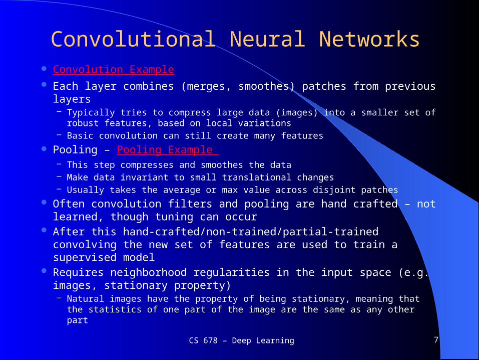
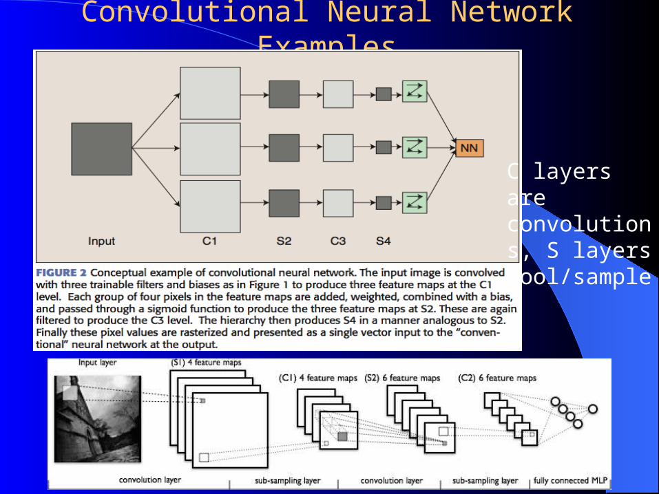
Training Deep Networks
Build a feature spacendash Note that this is what we do with SVM kernels or trained hidden
layers in BP etc but now we will build the feature space using deep architectures
ndash Unsupervised training between layers can decompose the problem into distributed sub-problems (with higher levels of abstraction) to be further decomposed at subsequent layers
CS 678 ndash Deep Learning 9
Training Deep Networks
Difficulties of supervised training of deep networksndash Early layers of MLP do not get trained well
Diffusion of Gradient ndash error attenuates as it propagates to earlier layers Leads to very slow training Exacerbated since top couple layers can usually learn any task pretty
well and thus the error to earlier layers drops quickly as the top layers mostly solve the taskndash lower layers never get the opportunity to use their capacity to improve results they just do a random feature map
Need a way for early layers to do effective workndash Often not enough labeled data available while there may be lots of
unlabeled data Can we use unsupervisedsemi-supervised approaches to take advantage
of the unlabeled datandash Deep networks tend to have more local minima problems than
shallow networks during supervised training
CS 678 ndash Deep Learning 10
Greedy Layer-Wise Training
One answer is greedy layer-wise training
1 Train first layer using your data without the labels (unsupervised)ndash Since there are no targets at this level labels dont help Could also use the
more abundant unlabeled data which is not part of the training set (ie self-taught learning)
2 Then freeze the first layer parameters and start training the second layer using the output of the first layer as the unsupervised input to the second layer
3 Repeat this for as many layers as desiredndash This builds our set of robust features
4 Use the outputs of the final layer as inputs to a supervised layermodel and train the last supervised layer(s) (leave early weights frozen)
5 Unfreeze all weights and fine tune the full network by training with a supervised approach given the pre-processed weight settings
CS 678 ndash Deep Learning 11
Deep Net with Greedy Layer Wise Training
Adobe ndash Deep Learning and Active Learning 12
ML Model
New Feature Space
Original Inputs
SupervisedLearning
UnsupervisedLearning
Greedy Layer-Wise Training
Greedy layer-wise training avoids many of the problems of trying to train a deep net in a supervised fashionndash Each layer gets full learning focus in its turn since it is the only
current top layerndash Can take advantage of unlabeled datandash When you finally tune the entire network with supervised training
the network weights have already been adjusted so that you are in a good error basin and just need fine tuning This helps with problems of
Ineffective early layer learning Deep network local minima
We will discuss the two most common approachesndash Stacked Auto-Encodersndash Deep Belief Networks
CS 678 ndash Deep Learning 13
Self Taught vs Unsupervised Learning
When using Unsupervised Learning as a pre-processor to supervised learning you are typically given examples from the same distribution as the later supervised instances will come fromndash Assume the distribution comes from a set containing just examples from a
defined set up possible output classes but the label is not available (eg images of car vs trains vs motorcycles)
In Self-Taught Learning we do not require that the later supervised instances come from the same distributionndash eg Do self-taught learning with any images even though later you will do
supervised learning with just cars trains and motorcyclesndash These types of distributions are more readily available than ones which just have
the classes of interestndash However if distributions are very differenthellip
New tasks share conceptsfeatures from existing data and statistical regularities in the input distribution that many tasks can benefit fromndash Note similarities to supervised multi-task and transfer learning
Both approaches reasonable in deep learning modelsCS 678 ndash Deep Learning 14
Auto-Encoders A type of unsupervised learning which tries to discover generic
features of the datandash Learn identity function by learning important sub-features (not by just passing
through data)ndash Compression etcndash Can use just new features in the new training set or concatenate both
15
Stacked Auto-Encoders Bengio (2007) ndash After Deep Belief Networks (2006) Stack many (sparse) auto-encoders in succession and train them using
greedy layer-wise training Drop the decode output layer each time
CS 678 ndash Deep Learning 16
Stacked Auto-Encoders Do supervised training on the last layer using final features Then do supervised training on the entire network to fine-
tune all weights
17
Sparse Encoders Auto encoders will often do a dimensionality reduction
ndash PCA-like or non-linear dimensionality reduction This leads to a dense representation which is nice in terms of
parsimonyndash All features typically have non-zero values for any input and the
combination of values contains the compressed information However this distributed and entangled representation can often
make it more difficult for successive layers to pick out the salient features
A sparse representation uses more features where at any given time a significant number of the features will have a 0 valuendash This leads to more localist variable length encodings where a particular
node (or small group of nodes) with value 1 signifies the presence of a feature (small set of bases)
ndash A type of simplicity bottleneck (regularizer)ndash This is easier for subsequent layers to use for learning
CS 678 ndash Deep Learning 18
How do we implement a sparse Auto-Encoder
Use more hidden nodes in the encoder Use regularization techniques which encourage sparseness
(eg a significant portion of nodes have 0 output for any given input)ndash Penalty in the learning function for non-zero nodesndash Weight decayndash etc
De-noising Auto-Encoderndash Stochastically corrupt training instance each time but still train
auto-encoder to decode the uncorrupted instance forcing it to learn conditional dependencies within the instance
ndash Better empirical results handles missing values well
CS 678 ndash Deep Learning 19
Sparse Representation For bases below which is easier to see intuition for current
pattern - if a few of these are on and the rest 0 or if all have some non-zero value
Easier to learn if sparse
CS 678 ndash Deep Learning 20
Stacked Auto-Encoders
Concatenation approach (ie using both hidden features and original features in final (or other) layers) can be better if not doing fine tuning If fine tuning the pure replacement approach can work well
Always fine tune if there is a sufficient amount of labeled data For real valued inputs MLP training is like regression and thus
could use linear output node activations still sigmoid at hidden
Stacked Auto-Encoders empirically not quite as accurate as DBNs (Deep Belief Networks)ndash (with De-noising auto-encoders stacked auto-encoders competitive
with DBNs)ndash Not generative like DBNs though recent work with de-noising auto-
encoders may allow generative capacity
CS 678 ndash Deep Learning 21
Deep Belief Networks (DBN)
Geoff Hinton (2006) Uses Greedy layer-wise training but each layer is an RBM
(Restricted Boltzmann Machine) RBM is a constrained
Boltzmann machine withndash No lateral connections between
hidden (h) and visible (x) nodesndash Symmetric weightsndash Does not use annealingtemperature but that is all right since each
RBM not seeking a global minima but rather an incremental transformation of the feature space
ndash Typically uses probabilistic logistic node but other activations possible
CS 678 ndash Deep Learning 22
RBM Sampling and Training
Initial state typically set to a training
example x (can be real valued) Sampling is an iterative back and forth process
ndash P(hi = 1|x) = sigmoid(Wix + ci) = 1(1+e-net(hi)) ci is hidden node bias
ndash P(xi = 1|h) = sigmoid(Wih + bi) = 1(1+e-net(xi)) bi is visible node bias
Contrastive Divergence (CD-k) How much contrast (in the statistical distribution) is there in the divergence from the original training example to the relaxed version after k relaxation steps
Then update weights to decrease the divergence as in Boltzmann Typically just do CD-1 (Good empirical results)
ndash Since small learning rate doing many of these is similar to doing fewer versions of CD-k with k gt 1
ndash Note CD-1 just needs to get the gradient direction right which it usually does and then change weights in that direction according to the learning rate
CS 678 ndash Deep Learning 23
24
RBM Update Notes and Variations
Binomial unit means the standard MLP sigmoid unit Q and P are probability distribution vectors for hidden (h)
and visibleinput (x) vectors respectively During relaxationweight update can alternatively do
updates based on the real valued probabilities (sigmoid(net)) rather than the 10 sampled logistic statesndash Always use actualbinary values from initial x -gt h
Doing this makes the hidden nodes a sparser bottleneck and is a regularizer helping to avoid overfit
ndash Could use probabilities on the h -gt x andor final x -gt h in CD-k the final update of the hidden nodes usually use the
probability value to decrease the final arbitrary sampling variation (sampling noise)
Lateral restrictions of RBM allow this fast samplingCS 678 ndash Deep Learning 25
RBM Update Variations and Notes
Initial weights small random 0 mean sd ~ 01ndash Dont want hidden node probabilities early on to be close to 0 or 1
else slows learning since less early randomnessmixing Note that this is a bit like annealingtemperature in Boltzmann
Set initial x bias values as a function of how often node is on in the training data and h biases to 0 or negative to encourage sparsity
Better speed when using momentum (~5) Weight decay good for smoothing and also encouraging
more mixing (hidden nodes more stochastic when they do not have large net magnitudes)ndash Also a reason to increase k over time in CD-k as mixing decreases
as weight magnitudes increase
CS 678 ndash Deep Learning 26
Deep Belief Network Training
Same greedy layer-wise approach First train lowest RBM (h0 ndash h1) using
RBM update algorithm (note h0 is x) Freeze weights and train subsequent
RBM layers Then connect final outputs to a
supervised model and train that model
Finally unfreeze all weights and train full DBN with supervised model to fine-tune weights
CS 678 ndash Deep Learning 27
During execution typically iterate multiple times at the top RBM layer
Can use DBN as a Generative model to create sample x vectors1 Initialize top layer to an arbitrary vector
Gibbs sample (relaxation) between the top two layers m times If we initialize top layer with values obtained from a training example then
need less Gibbs samples
2 Pass the vector down through the network sampling with the calculated probabilities at each layer
3 Last sample at bottom is the generated x value (can be real valued if we use the probability vector rather than sample)
Alternatively can start with an x at the bottom relax to a top value then start from that vector when generating a new x which is the dotted lines version More like standard Boltzmann machine processing
28
29
DBN Execution
After all layers have learned then the output of the last layer can be input to a supervised learning model
Note that at this point we could potentially throw away all the downward weights in the network as they will not actually be used during the normal feedforward execution process (as we did with the Stacked Auto Encoder)ndash Note that except for the downward bias weights b they are the same
symmetric weights anywaysndash If we are relaxing M times in the top layer then we would still need
the downward weights for that layerndash Also if we are generating x values we would need all of them
The final weight tuning is usually done with backpropagation which only updates the feedforward weights ignoring any downward weights
CS 678 ndash Deep Learning 30
DBN Learning Notes RBM stopping criteria still in issue One common approach is
reconstruction error which is the probability that the final x after CD-k is the initial x (ie P(1113088x|E[h|x1113088]) The other most common approach is AIC (Annealed Importance Sampling) Both have been shown to be problematic
Each layer updates weights so as to make training sample patterns more likely (lower energy) in the free state (and non-training sample patterns less likely)
This unsupervised approach learns broad features (in the hiddensubsequent layers of RBMs) which can aid in the process of making the types of patterns found in the training set more likely This discovers features which can be associated across training patterns and thus potentially helpful for other goals with the training set (classification compression etc)
Note still pairwise weights in RBMs but because we can pick the number of hidden units and layers we can represent any arbitrary distribution
CS 678 ndash Deep Learning 31
MNIST
CS 678 ndash Deep Learning 32
DBN Project Notes To be consistent just use 28times28 (764) data set of gray scale
values (0-255)ndash Normalize to 0-1ndash Could try better preprocessing if want and helps in published
accuracies but startstay with thisndash Small random initial weights
Parametersndash Hinton Paper others ndash do a little searching and e-mail me a
reference for extra credit pointsndash httpyannlecuncomexdbmnist for sample approaches
Straight 200 hidden node MLP does quite good 98-982 Best class deep net results ~985 - which is competitive
ndash About half students never beat MLP baselinendash Can you beat the 985
CS 678 ndash Deep Learning 33
Deep Learning Project Past Experience Structure ~3 hidden layers ~500ish nodeslayer more nodes
better but training is longer Training time
ndash DBN At least 10 epochs with the 60K setndash Can go longer does not seem to overfit with the large data setndash SAE Can overfit 3 epochs good but will be a function of your de-
noising approach which is essential for sparsity
Sampling vs using real probability value in DBNndash Best results found when using real values vs samplingndash Some found sampling on the back-step of learning helpsndash When using sampling probably requires longer training but could
actually lead to bigger improvements in the long runndash Typical forward flow real during execution but could do some sampling
on the m iterations at the top layer Some success with back-step at the top layer iteration (most dont do this at all)
ndash We need to trydiscover better variations
CS 678 ndash Deep Learning 34
Deep Learning Project Past Experience
Note If we held out 50K of the dataset as unsupervised then deep nets would more readily show noticeable improvement over BP
A final full network fine tune with BP always helpsndash But can take 20+ hours
Key take away ndash Most actual time spent training with different parameters Thus start early and then you will have time to try multiple long runs to see which variations work This does not take that much personal time as you simply start it with some different parameters and go away for a day If you wait until the last few days there is no time to do these experiments
CS 678 ndash Deep Learning 35
DBN Notes
Can use lateral connections in RBM (no longer RBM) but sampling becomes more difficult ndash ala standard Boltzmann requiring longer sampling chainsndash Lateral connections can capture pairwise dependencies allowing the hidden
nodes to focus on higher order issues Can get better results
Deep Boltzmann machine ndash Allow continual relaxation across the full networkndash Receive input from above and below rather than sequence through RBM
layersndash Typically for successful training first initialize weights using the standard
greedy DBN training with RBM layersndash Requires longer sampling chains ala Boltzmann
Conditional and Temporal RBMs ndash allow node probabilities to be conditioned by some other inputs ndash context recurrence (time series changes in input and internal state) etc
CS 678 ndash Deep Learning 36
Discrimination with Deep Networks Discrimination approaches with DBNs (Deep Belief Net)
ndash Use outputs of DBNs as inputs to supervised model (ie just an unsupervised preprocessor for feature extraction)
Basic approach we have been discussingndash Train a DBN for each class For each clamp the unknown x and
iterate m times The DBN that ends with the lowest normalized free energy (softmax variation) is the winner
ndash Train just one DBN for all classes but with an additional visible unit for each class For each output class
Clamp the unknown x relax and then see which final state has lowest free energy ndash no need to normalize since all energies come from the same network
See httpdeeplearningnetdemos
CS 678 ndash Deep Learning 37
Conclusion
Much recent excitement still much to be discovered Google-Brain Sum of Products Nets Biological Plausibility Potential for significant improvements Good in structuredMarkovian spaces
ndash Important research question To what extent can we use Deep Learning in more arbitrary feature spaces
ndash Recent deep training of MLPs with BP shows potential in this area
CS 678 ndash Deep Learning 38
- Deep Learning
- Deep Learning Overview
- Deep Learning Tasks
- Why Deep Learning
- Early Work
- BP Training Problems
- Convolutional Neural Networks
- Convolutional Neural Network Examples
- Training Deep Networks
- Training Deep Networks (2)
- Greedy Layer-Wise Training
- Deep Net with Greedy Layer Wise Training
- Greedy Layer-Wise Training (2)
- Self Taught vs Unsupervised Learning
- Auto-Encoders
- Stacked Auto-Encoders
- Stacked Auto-Encoders (2)
- Sparse Encoders
- How do we implement a sparse Auto-Encoder
- Sparse Representation
- Stacked Auto-Encoders (3)
- Deep Belief Networks (DBN)
- RBM Sampling and Training
- Slide 24
- RBM Update Notes and Variations
- RBM Update Variations and Notes
- Deep Belief Network Training
- Slide 28
- Slide 29
- DBN Execution
- DBN Learning Notes
- MNIST
- DBN Project Notes
- Deep Learning Project Past Experience
- Deep Learning Project Past Experience (2)
- DBN Notes
- Discrimination with Deep Networks
- Conclusion
-
Greedy Layer-Wise Training
One answer is greedy layer-wise training
1 Train first layer using your data without the labels (unsupervised)ndash Since there are no targets at this level labels dont help Could also use the
more abundant unlabeled data which is not part of the training set (ie self-taught learning)
2 Then freeze the first layer parameters and start training the second layer using the output of the first layer as the unsupervised input to the second layer
3 Repeat this for as many layers as desiredndash This builds our set of robust features
4 Use the outputs of the final layer as inputs to a supervised layermodel and train the last supervised layer(s) (leave early weights frozen)
5 Unfreeze all weights and fine tune the full network by training with a supervised approach given the pre-processed weight settings
CS 678 ndash Deep Learning 11
Deep Net with Greedy Layer Wise Training
Adobe ndash Deep Learning and Active Learning 12
ML Model
New Feature Space
Original Inputs
SupervisedLearning
UnsupervisedLearning
Greedy Layer-Wise Training
Greedy layer-wise training avoids many of the problems of trying to train a deep net in a supervised fashionndash Each layer gets full learning focus in its turn since it is the only
current top layerndash Can take advantage of unlabeled datandash When you finally tune the entire network with supervised training
the network weights have already been adjusted so that you are in a good error basin and just need fine tuning This helps with problems of
Ineffective early layer learning Deep network local minima
We will discuss the two most common approachesndash Stacked Auto-Encodersndash Deep Belief Networks
CS 678 ndash Deep Learning 13
Self Taught vs Unsupervised Learning
When using Unsupervised Learning as a pre-processor to supervised learning you are typically given examples from the same distribution as the later supervised instances will come fromndash Assume the distribution comes from a set containing just examples from a
defined set up possible output classes but the label is not available (eg images of car vs trains vs motorcycles)
In Self-Taught Learning we do not require that the later supervised instances come from the same distributionndash eg Do self-taught learning with any images even though later you will do
supervised learning with just cars trains and motorcyclesndash These types of distributions are more readily available than ones which just have
the classes of interestndash However if distributions are very differenthellip
New tasks share conceptsfeatures from existing data and statistical regularities in the input distribution that many tasks can benefit fromndash Note similarities to supervised multi-task and transfer learning
Both approaches reasonable in deep learning modelsCS 678 ndash Deep Learning 14
Auto-Encoders A type of unsupervised learning which tries to discover generic
features of the datandash Learn identity function by learning important sub-features (not by just passing
through data)ndash Compression etcndash Can use just new features in the new training set or concatenate both
15
Stacked Auto-Encoders Bengio (2007) ndash After Deep Belief Networks (2006) Stack many (sparse) auto-encoders in succession and train them using
greedy layer-wise training Drop the decode output layer each time
CS 678 ndash Deep Learning 16
Stacked Auto-Encoders Do supervised training on the last layer using final features Then do supervised training on the entire network to fine-
tune all weights
17
Sparse Encoders Auto encoders will often do a dimensionality reduction
ndash PCA-like or non-linear dimensionality reduction This leads to a dense representation which is nice in terms of
parsimonyndash All features typically have non-zero values for any input and the
combination of values contains the compressed information However this distributed and entangled representation can often
make it more difficult for successive layers to pick out the salient features
A sparse representation uses more features where at any given time a significant number of the features will have a 0 valuendash This leads to more localist variable length encodings where a particular
node (or small group of nodes) with value 1 signifies the presence of a feature (small set of bases)
ndash A type of simplicity bottleneck (regularizer)ndash This is easier for subsequent layers to use for learning
CS 678 ndash Deep Learning 18
How do we implement a sparse Auto-Encoder
Use more hidden nodes in the encoder Use regularization techniques which encourage sparseness
(eg a significant portion of nodes have 0 output for any given input)ndash Penalty in the learning function for non-zero nodesndash Weight decayndash etc
De-noising Auto-Encoderndash Stochastically corrupt training instance each time but still train
auto-encoder to decode the uncorrupted instance forcing it to learn conditional dependencies within the instance
ndash Better empirical results handles missing values well
CS 678 ndash Deep Learning 19
Sparse Representation For bases below which is easier to see intuition for current
pattern - if a few of these are on and the rest 0 or if all have some non-zero value
Easier to learn if sparse
CS 678 ndash Deep Learning 20
Stacked Auto-Encoders
Concatenation approach (ie using both hidden features and original features in final (or other) layers) can be better if not doing fine tuning If fine tuning the pure replacement approach can work well
Always fine tune if there is a sufficient amount of labeled data For real valued inputs MLP training is like regression and thus
could use linear output node activations still sigmoid at hidden
Stacked Auto-Encoders empirically not quite as accurate as DBNs (Deep Belief Networks)ndash (with De-noising auto-encoders stacked auto-encoders competitive
with DBNs)ndash Not generative like DBNs though recent work with de-noising auto-
encoders may allow generative capacity
CS 678 ndash Deep Learning 21
Deep Belief Networks (DBN)
Geoff Hinton (2006) Uses Greedy layer-wise training but each layer is an RBM
(Restricted Boltzmann Machine) RBM is a constrained
Boltzmann machine withndash No lateral connections between
hidden (h) and visible (x) nodesndash Symmetric weightsndash Does not use annealingtemperature but that is all right since each
RBM not seeking a global minima but rather an incremental transformation of the feature space
ndash Typically uses probabilistic logistic node but other activations possible
CS 678 ndash Deep Learning 22
RBM Sampling and Training
Initial state typically set to a training
example x (can be real valued) Sampling is an iterative back and forth process
ndash P(hi = 1|x) = sigmoid(Wix + ci) = 1(1+e-net(hi)) ci is hidden node bias
ndash P(xi = 1|h) = sigmoid(Wih + bi) = 1(1+e-net(xi)) bi is visible node bias
Contrastive Divergence (CD-k) How much contrast (in the statistical distribution) is there in the divergence from the original training example to the relaxed version after k relaxation steps
Then update weights to decrease the divergence as in Boltzmann Typically just do CD-1 (Good empirical results)
ndash Since small learning rate doing many of these is similar to doing fewer versions of CD-k with k gt 1
ndash Note CD-1 just needs to get the gradient direction right which it usually does and then change weights in that direction according to the learning rate
CS 678 ndash Deep Learning 23
24
RBM Update Notes and Variations
Binomial unit means the standard MLP sigmoid unit Q and P are probability distribution vectors for hidden (h)
and visibleinput (x) vectors respectively During relaxationweight update can alternatively do
updates based on the real valued probabilities (sigmoid(net)) rather than the 10 sampled logistic statesndash Always use actualbinary values from initial x -gt h
Doing this makes the hidden nodes a sparser bottleneck and is a regularizer helping to avoid overfit
ndash Could use probabilities on the h -gt x andor final x -gt h in CD-k the final update of the hidden nodes usually use the
probability value to decrease the final arbitrary sampling variation (sampling noise)
Lateral restrictions of RBM allow this fast samplingCS 678 ndash Deep Learning 25
RBM Update Variations and Notes
Initial weights small random 0 mean sd ~ 01ndash Dont want hidden node probabilities early on to be close to 0 or 1
else slows learning since less early randomnessmixing Note that this is a bit like annealingtemperature in Boltzmann
Set initial x bias values as a function of how often node is on in the training data and h biases to 0 or negative to encourage sparsity
Better speed when using momentum (~5) Weight decay good for smoothing and also encouraging
more mixing (hidden nodes more stochastic when they do not have large net magnitudes)ndash Also a reason to increase k over time in CD-k as mixing decreases
as weight magnitudes increase
CS 678 ndash Deep Learning 26
Deep Belief Network Training
Same greedy layer-wise approach First train lowest RBM (h0 ndash h1) using
RBM update algorithm (note h0 is x) Freeze weights and train subsequent
RBM layers Then connect final outputs to a
supervised model and train that model
Finally unfreeze all weights and train full DBN with supervised model to fine-tune weights
CS 678 ndash Deep Learning 27
During execution typically iterate multiple times at the top RBM layer
Can use DBN as a Generative model to create sample x vectors1 Initialize top layer to an arbitrary vector
Gibbs sample (relaxation) between the top two layers m times If we initialize top layer with values obtained from a training example then
need less Gibbs samples
2 Pass the vector down through the network sampling with the calculated probabilities at each layer
3 Last sample at bottom is the generated x value (can be real valued if we use the probability vector rather than sample)
Alternatively can start with an x at the bottom relax to a top value then start from that vector when generating a new x which is the dotted lines version More like standard Boltzmann machine processing
28
29
DBN Execution
After all layers have learned then the output of the last layer can be input to a supervised learning model
Note that at this point we could potentially throw away all the downward weights in the network as they will not actually be used during the normal feedforward execution process (as we did with the Stacked Auto Encoder)ndash Note that except for the downward bias weights b they are the same
symmetric weights anywaysndash If we are relaxing M times in the top layer then we would still need
the downward weights for that layerndash Also if we are generating x values we would need all of them
The final weight tuning is usually done with backpropagation which only updates the feedforward weights ignoring any downward weights
CS 678 ndash Deep Learning 30
DBN Learning Notes RBM stopping criteria still in issue One common approach is
reconstruction error which is the probability that the final x after CD-k is the initial x (ie P(1113088x|E[h|x1113088]) The other most common approach is AIC (Annealed Importance Sampling) Both have been shown to be problematic
Each layer updates weights so as to make training sample patterns more likely (lower energy) in the free state (and non-training sample patterns less likely)
This unsupervised approach learns broad features (in the hiddensubsequent layers of RBMs) which can aid in the process of making the types of patterns found in the training set more likely This discovers features which can be associated across training patterns and thus potentially helpful for other goals with the training set (classification compression etc)
Note still pairwise weights in RBMs but because we can pick the number of hidden units and layers we can represent any arbitrary distribution
CS 678 ndash Deep Learning 31
MNIST
CS 678 ndash Deep Learning 32
DBN Project Notes To be consistent just use 28times28 (764) data set of gray scale
values (0-255)ndash Normalize to 0-1ndash Could try better preprocessing if want and helps in published
accuracies but startstay with thisndash Small random initial weights
Parametersndash Hinton Paper others ndash do a little searching and e-mail me a
reference for extra credit pointsndash httpyannlecuncomexdbmnist for sample approaches
Straight 200 hidden node MLP does quite good 98-982 Best class deep net results ~985 - which is competitive
ndash About half students never beat MLP baselinendash Can you beat the 985
CS 678 ndash Deep Learning 33
Deep Learning Project Past Experience Structure ~3 hidden layers ~500ish nodeslayer more nodes
better but training is longer Training time
ndash DBN At least 10 epochs with the 60K setndash Can go longer does not seem to overfit with the large data setndash SAE Can overfit 3 epochs good but will be a function of your de-
noising approach which is essential for sparsity
Sampling vs using real probability value in DBNndash Best results found when using real values vs samplingndash Some found sampling on the back-step of learning helpsndash When using sampling probably requires longer training but could
actually lead to bigger improvements in the long runndash Typical forward flow real during execution but could do some sampling
on the m iterations at the top layer Some success with back-step at the top layer iteration (most dont do this at all)
ndash We need to trydiscover better variations
CS 678 ndash Deep Learning 34
Deep Learning Project Past Experience
Note If we held out 50K of the dataset as unsupervised then deep nets would more readily show noticeable improvement over BP
A final full network fine tune with BP always helpsndash But can take 20+ hours
Key take away ndash Most actual time spent training with different parameters Thus start early and then you will have time to try multiple long runs to see which variations work This does not take that much personal time as you simply start it with some different parameters and go away for a day If you wait until the last few days there is no time to do these experiments
CS 678 ndash Deep Learning 35
DBN Notes
Can use lateral connections in RBM (no longer RBM) but sampling becomes more difficult ndash ala standard Boltzmann requiring longer sampling chainsndash Lateral connections can capture pairwise dependencies allowing the hidden
nodes to focus on higher order issues Can get better results
Deep Boltzmann machine ndash Allow continual relaxation across the full networkndash Receive input from above and below rather than sequence through RBM
layersndash Typically for successful training first initialize weights using the standard
greedy DBN training with RBM layersndash Requires longer sampling chains ala Boltzmann
Conditional and Temporal RBMs ndash allow node probabilities to be conditioned by some other inputs ndash context recurrence (time series changes in input and internal state) etc
CS 678 ndash Deep Learning 36
Discrimination with Deep Networks Discrimination approaches with DBNs (Deep Belief Net)
ndash Use outputs of DBNs as inputs to supervised model (ie just an unsupervised preprocessor for feature extraction)
Basic approach we have been discussingndash Train a DBN for each class For each clamp the unknown x and
iterate m times The DBN that ends with the lowest normalized free energy (softmax variation) is the winner
ndash Train just one DBN for all classes but with an additional visible unit for each class For each output class
Clamp the unknown x relax and then see which final state has lowest free energy ndash no need to normalize since all energies come from the same network
See httpdeeplearningnetdemos
CS 678 ndash Deep Learning 37
Conclusion
Much recent excitement still much to be discovered Google-Brain Sum of Products Nets Biological Plausibility Potential for significant improvements Good in structuredMarkovian spaces
ndash Important research question To what extent can we use Deep Learning in more arbitrary feature spaces
ndash Recent deep training of MLPs with BP shows potential in this area
CS 678 ndash Deep Learning 38
- Deep Learning
- Deep Learning Overview
- Deep Learning Tasks
- Why Deep Learning
- Early Work
- BP Training Problems
- Convolutional Neural Networks
- Convolutional Neural Network Examples
- Training Deep Networks
- Training Deep Networks (2)
- Greedy Layer-Wise Training
- Deep Net with Greedy Layer Wise Training
- Greedy Layer-Wise Training (2)
- Self Taught vs Unsupervised Learning
- Auto-Encoders
- Stacked Auto-Encoders
- Stacked Auto-Encoders (2)
- Sparse Encoders
- How do we implement a sparse Auto-Encoder
- Sparse Representation
- Stacked Auto-Encoders (3)
- Deep Belief Networks (DBN)
- RBM Sampling and Training
- Slide 24
- RBM Update Notes and Variations
- RBM Update Variations and Notes
- Deep Belief Network Training
- Slide 28
- Slide 29
- DBN Execution
- DBN Learning Notes
- MNIST
- DBN Project Notes
- Deep Learning Project Past Experience
- Deep Learning Project Past Experience (2)
- DBN Notes
- Discrimination with Deep Networks
- Conclusion
-
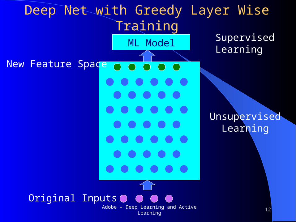
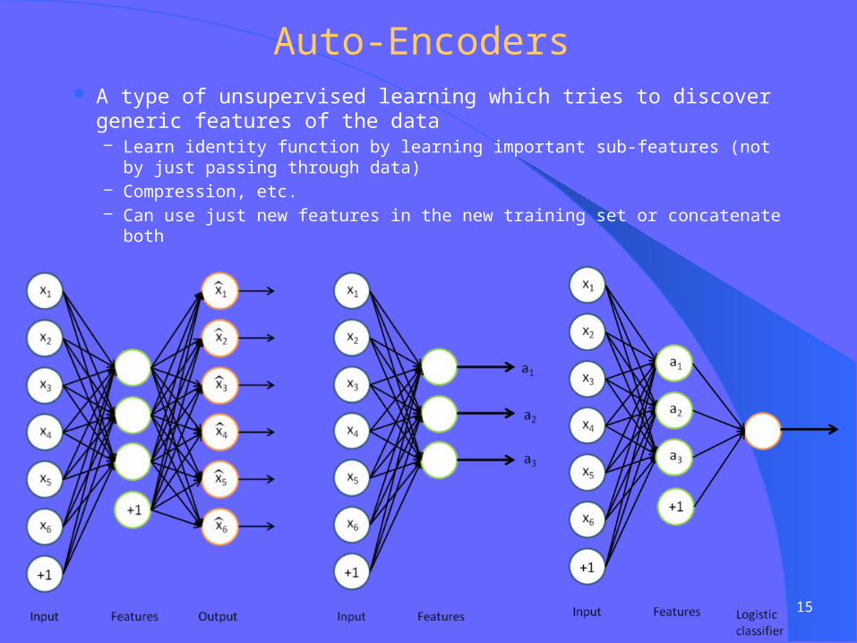
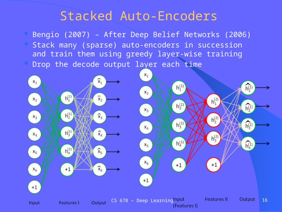
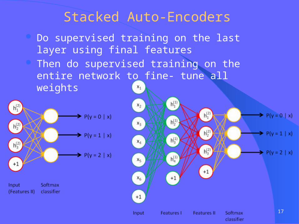
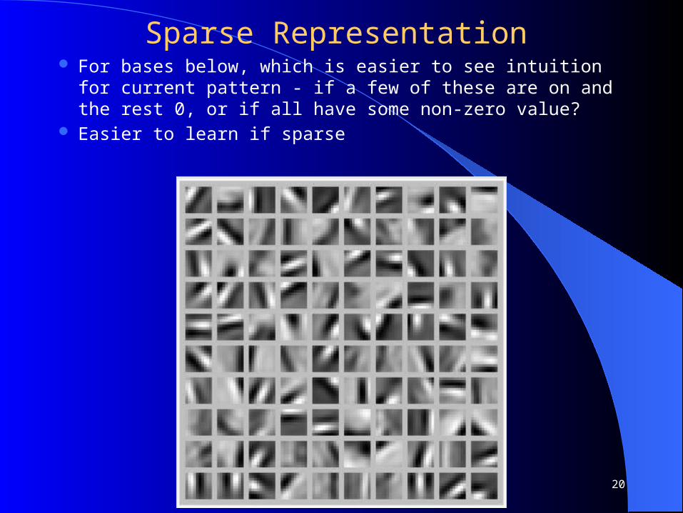
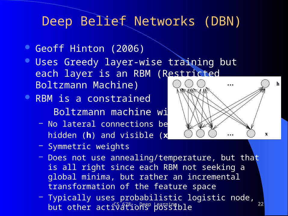
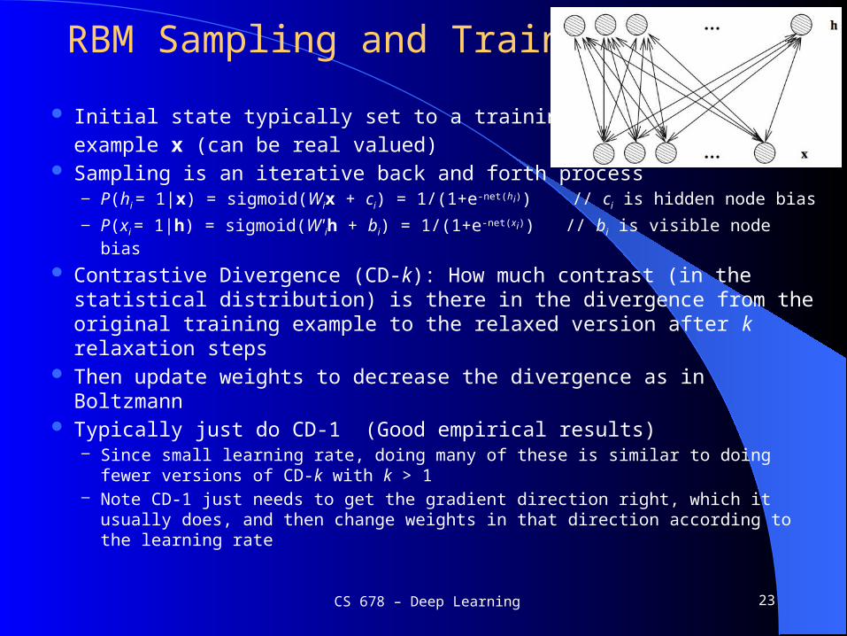
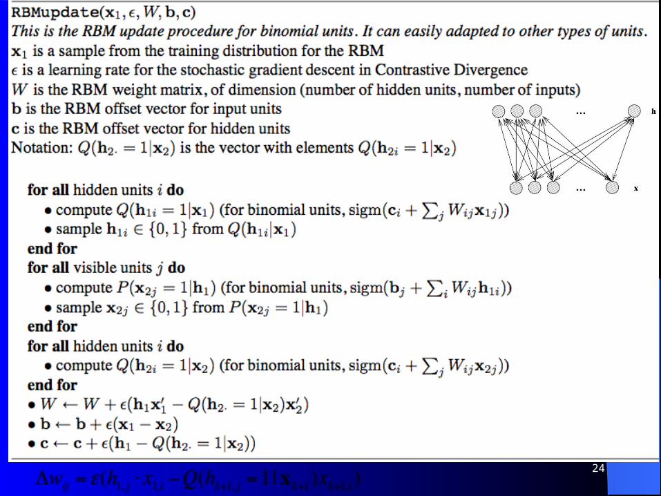
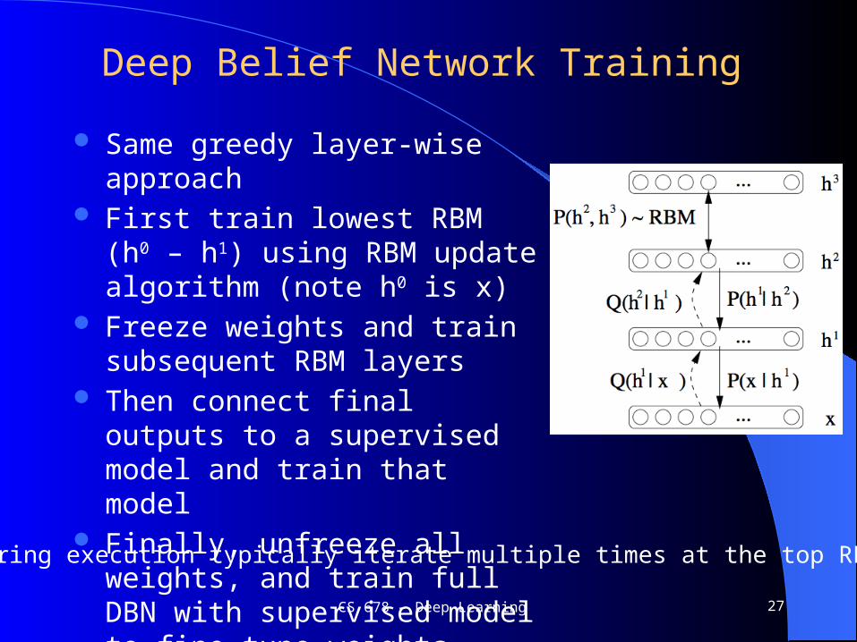
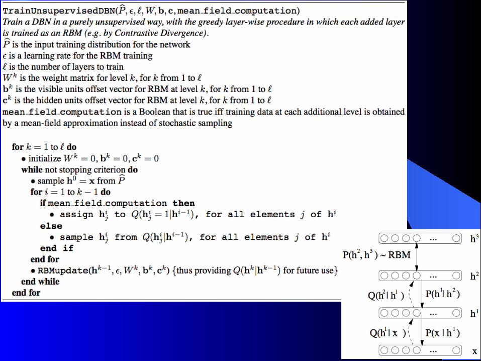
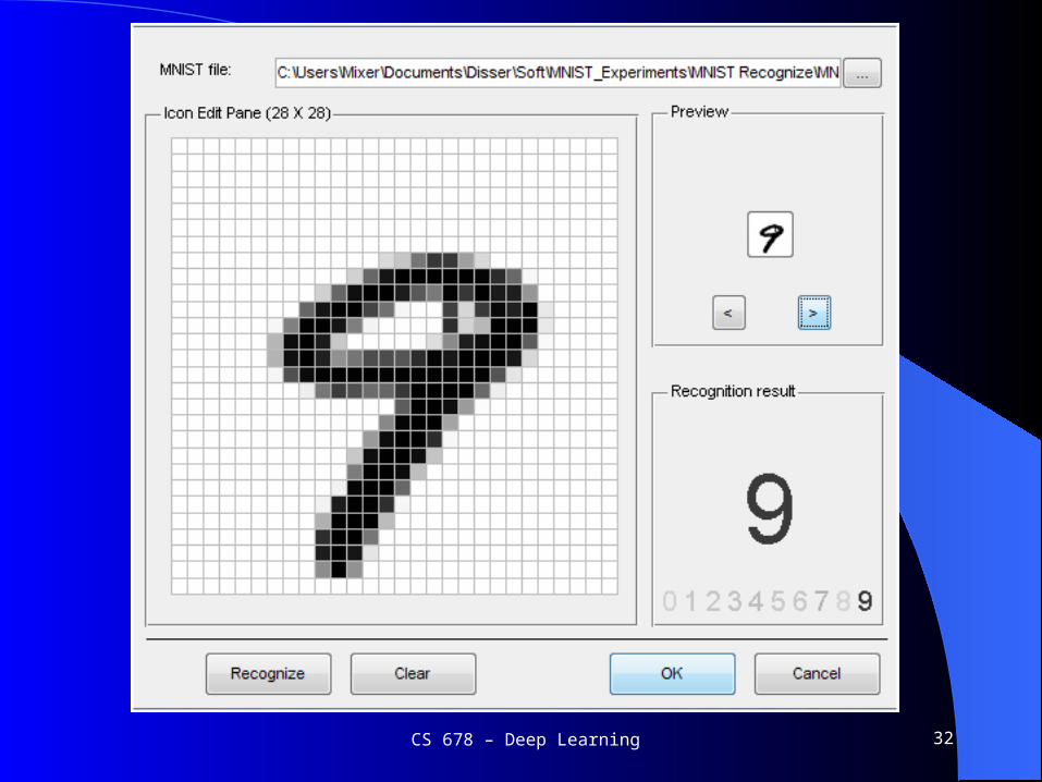
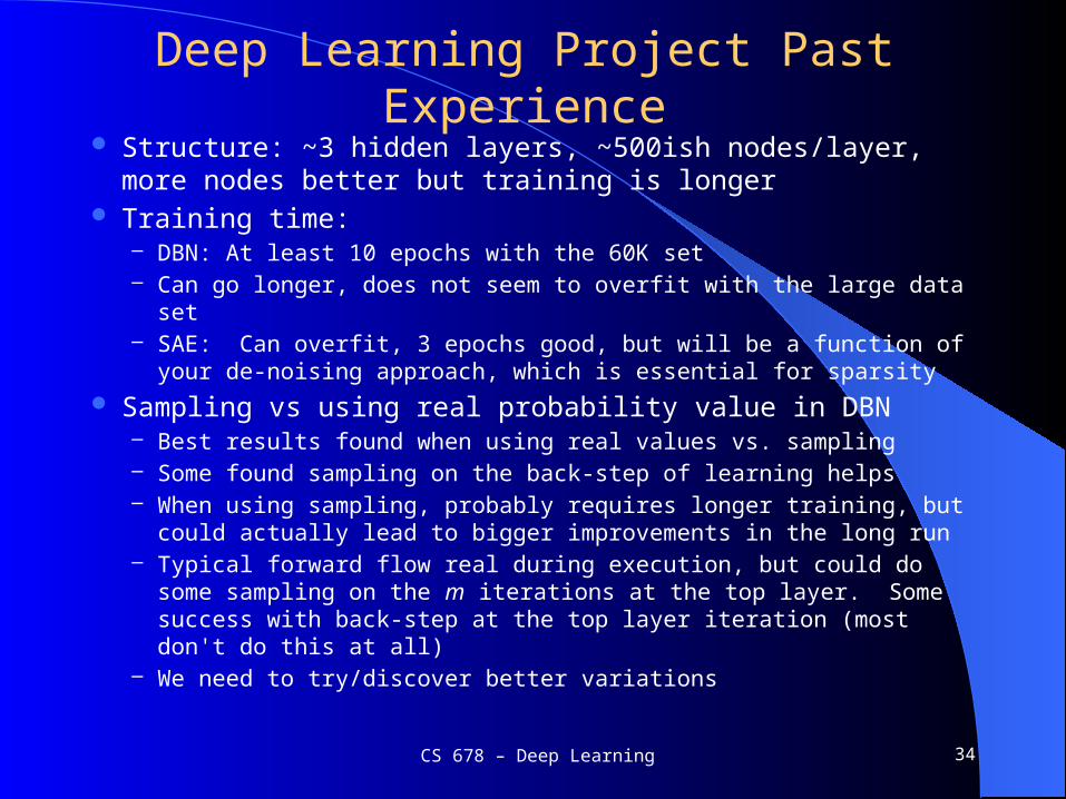