Research ArticleDeep Learning Enabled Fault Diagnosis Using Time-FrequencyImage Analysis of Rolling Element Bearings

David Verstraete1 Andreacutes Ferrada2 Enrique Loacutepez Droguett13

Viviana Meruane3 andMohammadModarres1

1Department of Mechanical Engineering University of Maryland College Park MD USA2Computer Science Department University of Chile Santiago Chile3Mechanical Engineering Department University of Chile Santiago Chile

Correspondence should be addressed to David Verstraete dbverstrterpmailumdedu

Received 13 May 2017 Accepted 14 August 2017 Published 9 October 2017

Academic Editor Matthew J Whelan

Copyright copy 2017 David Verstraete et al This is an open access article distributed under the Creative Commons AttributionLicense which permits unrestricted use distribution and reproduction in any medium provided the original work is properlycited

Traditional feature extraction and selection is a labor-intensive process requiring expert knowledge of the relevant features pertinentto the system This knowledge is sometimes a luxury and could introduce added uncertainty and bias to the results To addressthis problem a deep learning enabled featureless methodology is proposed to automatically learn the features of the data Time-frequency representations of the raw data are used to generate image representations of the raw signal which are then fed intoa deep convolutional neural network (CNN) architecture for classification and fault diagnosis This methodology was appliedto two public data sets of rolling element bearing vibration signals Three time-frequency analysis methods (short-time Fouriertransform wavelet transform and Hilbert-Huang transform) were explored for their representation effectiveness The proposedCNN architecture achieves better results with less learnable parameters than similar architectures used for fault detection includingcases with experimental noise

1 Introduction

With the proliferation of inexpensive sensing technology andthe advances in prognostics and health management (PHM)research customers are no longer requiring that their newasset investment be highly reliable instead they are requiringthat their assets possess the capability to diagnose faultsand provide alerts when components need to be replacedThese assets often have substantial sensor systems capableof generating millions of data points a minute Handlingthis amount of data often involves careful construction andextraction of features from the data to input into a predictivemodel Feature extraction relies on some prior knowledgeof the data Choosing which features to include or excludewithin the model is a continuous area of research without aset methodology to follow

Feature extraction and selection has opened a host ofopportunities for fault diagnosisThe transformation of a raw

signal into a feature vector allows the learning method toseparate classes and identify previously unknown patternswithin the dataThis has had wide ranging economic benefitsfor the owners of the assets and has opened new possibilitiesof revenue by allowing original equipment manufacturers(OEMs) to contract in maintainability and availability valueHowever the state of current diagnostics involves a laboriousprocess of creating a feature vector from the raw signal viafeature extraction [1ndash3] For example Seera proposes a Fuzzy-Min-Max Classification and Regression Tree (FMM-CART)model for diagnostics on Case Westernrsquos bearing data [4]Traditional feature extraction was completed within bothtime and frequency domains An important predictor-basedfeature selection measure was used to enhance the CARTmodel multilayer perceptron (MLP) was then applied to thefeatures for prediction accuracies

Once features are extracted traditional learning methodsare then applied to separate classify and predict faults from

HindawiShock and VibrationVolume 2017 Article ID 5067651 17 pageshttpsdoiorg10115520175067651

2 Shock and Vibration

learned patterns present within the layers of the featurevector [5 6] These layers of features are constructed byhuman engineers therefore they are subject to uncertaintyand biases of the domain experts creating these vectors Itis becoming more common that this process is performedon a set of massive multidimensional data Having priorknowledge of the features and representations within such adata set relevant to the patterns of interest is a challenge andis often only one layer deep

It is in this context that deep learning comes to playIndeed deep learning encompasses a set of representationlearning methods with multiple layers The primary benefitis the ability of the deep learning method to learn nonlin-ear representations of the raw signal to a higher level ofabstraction and complexity isolated from the touch of humanengineers directing the learning [7] For example to handlethe complexity of image classification convolutional neuralnetworks (ConvNets or CNNs) are the dominant method [8ndash13] In fact they are so dominant today that they rival humanaccuracies for the same tasks [14 15]

This is important from an engineering context becausecovariates often do not have a linear effect on the outcomeof the fault diagnosis Additionally there are situationswhere a covariate is not directly measured confounding whatcould be a direct effect on the asset The ability of deeplearning basedmethods to automatically construct nonlinearrepresentations given these situations is of great value to theengineering and fault diagnosis communities

Since 2015 deep learning methodologies have beenapplied with success to diagnostics or classification tasks ofrolling element signals [2 16ndash26] Wang et al [2] proposedthe use of wavelet scalogram images as an input into a CNNto detect faults within a set of vibration data A series of 32 times32 images is used Lee et al [20] explored a corrupted rawsignal and the effects of noise on the training of a CNNWhile not explicitly stated it appears that minimal dataconditioning bymeans of a short-time Fourier transformwascompleted and either images or a vector of these outputsindependent of time was used as the input layer to the CNNGuo et al [17] used Case Westernrsquos bearing data set [4] andan adaptive deep CNN to accomplish fault diagnosis andseverity Abdeljaber et al [19] used a CNN for structuraldamage detection on a grandstand simulator Janssens et al[21] incorporated shallow CNNs with the amplitudes of thediscrete Fourier transformvector of the raw signal as an inputPooling or subsampling layers were not used Chen et al [16]used traditional feature construction as a vector input to aCNN architecture consisting of one convolutional layer andone pooling layer for gearbox vibration data Although notdealing with rolling elements Zhang [22] used a deep learn-ing multiobjective deep belief network ensemble methodto estimate the remaining useful life of NASArsquos C-MAPSSdata set Liao et al [23] used restricted Boltzmann machines(RBMs) as a feature extraction method otherwise knownas transfer learning Feature selection was completed fromthe RBM output followed by a health assessment via self-organizingmaps (SOMs) the remaining useful life (RUL)wasthen estimated on run-to-failure data sets Babu [24] usedimages of two PHM competition data sets (C-MAPSS and

PHM 2008) as an input to a CNN architecture While thesedata sets did not involve rolling elements the feature mapswere time-based therefore allowing the piecewise remaininguseful life estimation Guo et al [18] incorporated traditionalfeature construction and extraction techniques to feed astacked autoencoder (SAE) deep neural network SAEs donot utilize convolutional and pooling layers Zhou et al [25]used fast Fourier transform on the CaseWestern bearing dataset for a vector input into a deep neural network (DNN)using 3 4 and 5 hidden layers DNNs do not incorporateconvolutional and pooling layers only hidden layers Liu etal [26] used spectrograms as input vectors into sparse andstacked autoencoders with two hidden layers Liursquos resultsindicate there was difficulty classifying outer race faultsversus the baseline Previous deep learning based modelsand applications to fault diagnostics are usually limited bytheir sensitivity to experimental noise or their reliance ontraditional feature extraction

In this paper we propose an improved CNN basedmodel architecture for time-frequency image analysis forfault diagnosis of rolling element bearings Its main elementconsists of a double layer CNN that is two consecutiveconvolutional layers without a pooling layer between themFurthermore two linear time-frequency transformations areused as image input to the CNN architecture short-timeFourier transform spectrogram and wavelet transform (WT)scalogram One nonlinear nonparametric time-frequencytransformation is also examined Hilbert-Huang transforma-tion (HHT) HHT is chosen to compliment the traditionaltime-frequency analysis of STFT and WT due to its benefitof not requiring the construction of a basis to match theraw signal components These three methods were chosenbecause they give suitable outputs for the discovery ofcomplex and high-dimensional representations without theneed for additional feature extraction Additionally HHTimages have not been used as a basis for fault diagnostics

Beyond the CNN architecture and three time-frequencyanalysis methods this paper also examines the loss ofinformation due to the scaling of images from 96 times 96to 32 times 32 pixels Image size has significant impact onthe CNNrsquos quantity of learnable parameters Training timeis less if the image size can be reduced but classificationaccuracy is negatively impacted The methodology is appliedto two public data sets (1) the Machinery Failure PreventionTechnology (MFPT) society rolling element vibrational dataset and (2) Case Western Reserve Universityrsquos Bearing dataset [4]

The rest of this paper is organized as follows Section 2provides an overview of deep learning and CNNs Section 3gives a brief overview of the time-frequency domain analysisincorporated into the image structures for the deep learningalgorithm to train Section 4 outlines the proposed CNNarchitecture constructed to accomplish the diagnostic taskof fault detection Sections 5 and 6 apply the methodol-ogy to two experimental data sets Comparisons of theproposed CNN architecture against MLP linear supportvector machine (SVM) and Gaussian SVM for both the rawdata and principal component mapping data are presentedAdditionally comparisons with Wang et al [2] proposed

Shock and Vibration 3

Input layer

Feature mapsFeature maps

Hidden layer

Output layer

Convolutional layer Pooling layer Fully connected layer

Figure 1 Generic CNN architecture

CNN architecture is presented Section 7 examines the dataset with traditional feature learning Section 8 explores theaddition of Gaussian noise to the signals Section 9 concludeswith discussion of the results

2 Deep Learning and CNN Background

Deep learning is representation learning however not allrepresentation learning is deep learning The most commonform of deep learning is supervised learningThat is the datais labeled prior to input into the algorithm Classificationor regression can be run against these labels and thuspredictions can be made from unlabeled inputs

Within the computer vision community there is one clearfavorite type of deep feedforward network that outperformedothers in generalizing and training networks consisting of fullconnectivity across adjacent layers the convolutional neuralnetwork (CNN) A CNNrsquos architecture is constructed as aseries of stages Each stage has a different role Each role iscompleted automatically within the algorithm Each architec-ture within the CNN construct consists of four propertiesmultiple layers poolingsubsampling shared weights andlocal connections

As shown in Figure 1 the first stage of a CNN is madeof two types of layers convolutional layers which organizethe units in feature maps and pooling layers which mergesimilar features into one feature Within the convolutionallayerrsquos featuremap each unit is connected to a previous layerrsquosfeature maps through a filter bank This filter consists of aset of weights and a corresponding local weighted sum Theweighted sum passed through a nonlinear function such as arectified linear unit (ReLU) This is shown in (1) ReLU is ahalf-wave rectifier 119891(119909) = max(119909 0) and is like the Softplusactivation function that is Softplus(119909) = ln(1 + 119890119909) ReLUactivation trains faster than the previously used sigmoidtanhfunctions [7]

X(119898)119896

= ReLU( 119862sum119888=1

W(119888119898)119896

lowast X(119888)119896minus1

+ B(119898)119896) (1)

where lowast represents the convolutional operator X(119888)119896minus1

is inputof convolutional channel 119888W(119888119898)

119896is filter weight matrixB(119898)

119896

is bias weight matrix ReLU is rectified linear unit

An important aspect of the convolutional layers for imageanalysis is that units within the same feature map share thesame filter bank However to handle the possibility thata feature maprsquos location is not the same for every imagedifferent feature maps use different filter banks [7] For imagerepresentations of vibration data this is important As featuresare extracted to characterize a given type of fault representedon the image it may be in different locations on subsequentimages It is worth noting that feature construction happensautomatically within the convolutional layer independent ofthe engineer constructing or selecting them which gives riseto the term featureless learning To be consistent with theterminology of the fault diagnosis community one couldliken the convolutional layer to a feature construction orextraction layer If a convolutional layer is similar in respectto feature construction the pooling layer in a CNN could berelated to a feature selection layer

The second stage of a CNN consists of a pooling layerto merge similar features into one This pooling or subsam-pling effectively reduces the dimensions of the representa-tion Mathematically the subsampling function 119891 is [27]

X(119898)119896

= 119891 (120573(119898)119896

down (X(119898minus1)119896

) + 119887(119898)119896

) (2)

where down (∙) represents the subsampling function 120573(119898)119896

ismultiplicative bias 119887(119898)

119896is additive bias

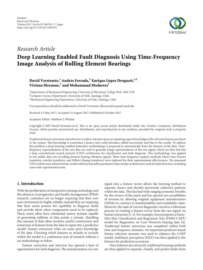
After multiple stacks of these layers are completed theoutput can be fed into the final stage of the CNN amultilayer perceptron (MLP) fully connected layer An MLPis a classification feedforward neural networkThe outputs ofthe final pooling layer are used as an input to map to labelsprovided for the data Therefore the analysis and predictionof vibration images are a series of representations of theraw signal For example the raw signal can be representedin a sinusoidal form via STFT STFT is then representedgraphically via a spectrogram and finally a CNN learns andclassifies the spectrogram image features and representationsthat best predict a classification based on a label Figure 2outlines how deep learning enabled feature learning differsfrom traditional feature learning

Traditional feature learning involves a process of con-structing features from the existing signal feature searching

4 Shock and Vibration

Feature construction

Feature selection (optional) Diagnostic model

Raw signal

Traditional feature learning

MeanStandard deviation

KurtosisSkewness

CrestRMS

Evaluation metrics

Filter methods

OptimumHeuristic

Wrapper method

Multilayer perceptronSupport vector machines

Neural networksDecision trees

Random forests

AccuracyConfusion matrix

PrecisionSpecificityF-measureSensitivity

Diagnostic model

Raw signal

Deep learning enabled feature learning

Evaluation metrics

STFTWavelets

HHTCNN

AccuracyPrecisionSpecificityF-measureSensitivity

Representation construction

SpectrogramsScalogramsHHT Plots

Figure 2 Process of representations for time-frequency analysis

via optimum or heuristic methods feature selection ofrelevant and important features via filter orwrappermethodsand feeding the resulting selected features into a classificationalgorithm Deep learning enabled feature learning has theadvantage of not requiring a feature construction searchand selection sequenceThis is done automatically within theframework of the CNN The strength of a CNN in its imageanalysis capabilities Therefore an image representation ofthe data as an input into the framework is ideal A vector inputof constructed features misses the intent and power of theCNN Given that the CNN searches spatially for features thesequence of the vector input can affect the resultsWithin thispaper spectrograms scalograms and HHT plots are used asthe image input to leverage the strengths of a CNN as shownin Figure 2

3 Time-Frequency MethodsDefinition and Discussion

Time frequency represents a signal in both the time andfrequency domains simultaneouslyThemost common time-frequency representations are spectrograms and scalogramsA spectrogram is a visual representation in the time-frequency domain of a signal using the STFT and a scalogramuses theWTThemain difference with both techniques is thatspectrograms have a fixed frequency resolution that dependson the windows size whereas scalograms have a frequency-dependent frequency resolution For low frequencies a longwindow is used to observe enough of the slow alternations inthe signal and at higher frequency values a shorter window is

used which results in a higher time resolution and a poorerfrequency resolution On the other hand the HHT doesnot divide the signal at fixed frequency components butthe frequency of the different components (IMFs) adapts tothe signal Therefore there is no reduction of the frequencyresolution by dividing the data into sections which givesHHT a higher time-frequency resolution than spectrogramsand scalograms In this paper we examine the representationeffectiveness of the following three methods STFT WT andHHT These representations will be graphically representedas an image and fed into the proposed CNN architecture inSection 4

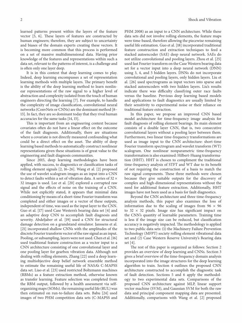
31 Spectrograms Short-Time Fourier Transform (STFT)Spectrograms are a visual representation of the STFT wherethe 119909- and 119910-axis are time and frequency respectively andthe color scale of the image indicates the amplitude of thefrequency The basis for the STFT representation is a seriesof sinusoids STFT is the most straightforward frequencydomain analysis However it cannot adequately model time-variant and transient signal Spectrograms add time to theanalysis of FFT allowing the localization of both time andfrequency Figure 3 illustrates a spectrogram for the baselinecondition of a rolling element bearing vibrational response

32 Scalograms Wavelet Transform Scalograms are a graph-ical image of the wavelet transform (WT) WTs are a lineartime-frequency representation with a wavelet basis insteadof sinusoidal functions Due to the addition of a scalevariable along with the time variable the WT is effective fornonstationary and transient signals

Shock and Vibration 5

minus120

minus100

minus80

minus60

minus40

minus20

1 15 205Time times10

5

0

01

02

03

04

05

06

07

08

09

1

Nor

mal

ized

freq

uenc

y (k

Hz)

Pow

erfr

eque

ncy

(dB

rad

sam

ple)

Figure 3 STFT spectrogram of baseline raw signal

times104

times10minus3

05

1

15

2

25

3

35

4

45

Freq

uenc

y (k

Hz)

05

1

15

2

Mag

nitu

de

002 004 006 008 01 0120Time (s)

Figure 4 Wavelet transform scalogram of baseline raw signal

For a wavelet transform WT119909(119887 119886) of a signal which isenergy limited 119909(119905) isin 1198712(119877) the basis for the transform canbe set as

WT119909 (119887 119886) = 1radic119886 int+infin

minusinfin

119909 (119905) 120595(119905 minus 119887119886 )119889119905 (3)

where 119886 is scale parameter 119887 is time parameter120595 is analyzingwavelet

Figure 4 illustrates a scalogram with a Morlet waveletbasis for the baseline condition of a rolling element bearingvibrational response There have been many studies onthe effectiveness of individual wavelets and their ability tomatch a signal One could choose between the GaussianMorlet Shannon Meyer Laplace Hermit or the MexicanHat wavelets in both simple and complex functions To datethere is not a defined methodology for identifying the properwavelet to be used and this remains an open question within

Signal

Empirical mode decomposition

Instantaneous amplitudes

Instantaneous frequencies

Intrinsic mode

functions

Hilbert transform

Hilbert-Huang

transform

Figure 5 Overview of HHT adapted fromWang (2010)

the research community [28] For the purposes of this paperthe Morlet wavelet Ψ120590(119905) is chosen because of its similarityto the impulse component of symptomatic faults of manymechanical systems [29] and is defined as

Ψ120590 (119905) = 119888120590120587minus(14)119890minus(12)1199052 (119890119894120590119905 minus 119870120590) (4)

where 119888 is normalization constant 119870120590 is admissibility crite-rion

Wavelets have been extensively used for machinery faultdiagnosis For the sake of brevity those interested can referto Peng and Chu [30] for a comprehensive review of thewavelet transformrsquos use within condition monitoring andfault diagnosis

33 Hilbert-Huang Transform Feng et al [28] refer to thetime-frequency analysis method Hilbert-Huang transform(HHT) as an adaptive nonparametric approach STFT andWT are limited in the sense that they are a representation ofthe raw signal on a predefined set of basis function HHTdoes not make predefined assumptions on the basis of thedata but employs the empirical mode decomposition (EMD)to decompose the signal into a set of elemental signals calledintrinsic mode functions (IMFs) The HHT methodology isdepicted in Figure 5

The HHT is useful for nonlinear and nonstationarytime series analysis which involves two steps EMD of thetime series signal and Hilbert spectrum construction It is

6 Shock and Vibration

005

01

015

02

025

03

0

1000

2000

3000

4000

5000

6000

Insta

ntan

eous

freq

uenc

y

5 10 15 200Time (seconds)

Figure 6 HHT image of baseline raw signal

an iterative numerical algorithm which approximates andextracts IMFs from the signal HHTs are particularly usefulfor localizing the properties of arbitrary signals For details ofthe complete HHT algorithm the reader is directed towardsHuang [31]

Figure 6 shows an HHT image of the raw baseline signalused in Figures 3 and 4 It is not uncommon for the HHTinstantaneous frequencies to return negative values Thisis because the HHT derives the instantaneous frequenciesfrom the local derivatives of the IMF phases The phase isnot restricted to monotonically increasing and can thereforedecrease for a timeThis results in a negative local derivativeFor further information regarding this property of HHT thereader is directed to read Meeson [32]

The EMD portion of the HHT algorithm suffers frompossible mode mixing Intermittences in signal can causethis Mode mixing within signals containing instantaneousfrequency trajectory crossings is inevitable The results ofmode mixing can result in erratic or negative instantaneousfrequencies [33] This means for such signals HHT doesnot outperform traditional time-frequency analysis methodssuch as STFT

4 Proposed CNN Architecture for FaultClassification Based on Vibration Signals

The primary element of the proposed architecture consists ofa double layer CNN that is two consecutive convolutionallayers without a pooling layer between themThe absence of apooling layer reduces the learnable parameters and increasesthe expressivity of the features via an additional nonlinearityHowever a pooling layer is inserted between two stackeddouble convolutional layers This part of the architecturemakes up the automatic feature extraction process that isthen followed by a fully connected layer to accomplish rollingelement fault detection

The first convolutional layer consists of 32 feature mapsof 3 times 3 size followed by second convolutional layer of 32feature maps of 3 times 3 size After this double convolutionallayer there is a pooling layer of 32 feature maps of 2 times 2size This makes up the first stage The second stage consists

of two convolutional layers of 64 feature maps each of 3times 3 size followed by subsampling layer of 64 feature mapsof 2 times 2 size The third stage consists of two convolutionallayers of 128 feature maps each of 3 times 3 size followed bysubsampling layer of 128 feature maps of 2 times 2 size Thelast two layers are fully connected layers of 100 featuresFigure 7 depicts this architecture The intent of two stackedconvolutional layers before a pooling layer is to get thebenefit of a large feature space via smaller features Thisconvolutional layer stacking has two advantages (1) reducingthe number of parameters the training stage must learn and(2) increasing the expressivity of the feature by adding anadditional nonlinearity

Table 1 provides an overview of CNN architectures thathave been used for fault diagnosis where Crsquos are convo-lutional layers Prsquos are pooling layers and FCs are fullyconnected layers The number preceding the C P and FCindicates the number of feature maps used The dimensions[3 times 3] and [2 times 2] indicate the pixel size of the features

Training the CNN involves the learning of all of theweights and biases present within the architectures Theseweights andbiases are referred to as learnable parametersThequantity of learnable parameters for a CNN architecture canradically improve or degrade the time to train of the modelTherefore it is important to optimize the learnable param-eters by balancing training time versus prediction accuracyTable 2 outlines the quantity of learnable parameters forthe proposed CNN architecture as well as a comparison toarchitectures 1 and 2 presented in Table 1

Beyond the learnable parameters the CNN requiresthe specification and optimization of the hyperparametersdropout and learning rate Dropout is an essential propertyof CNNs Dropout helps to prevent overfitting and reducetraining error and effectively thins the network (Srivastava2015) The remaining connections are comprised of all theunits that survive the dropout For this architecture dropoutis set to 05 For the other hyperparameter learning rate theadaptedmoment estimation (ADAM) algorithmwas used foroptimization It has had success in the optimizing the learningrate for CNNs faster than similar algorithms Instead of handpicking learning rates like similar algorithms the ADAMlearning rate scale adapts through different layers [34]

Part of the reason for deep learningrsquos recent success hasbeen the use of graphics processing unit (GPU) computing[7] GPU computing was used for this paper to increase thespeed and decrease the training time More specifically theprocessing system used for the analysis is as follows CPUCore i7-6700K 42GHz with 32GB ram and GPU Tesla K20

5 Case Study 1 Machinery FailurePrevention Technology

This data set was provided by the Machinery Failure Preven-tion Technology (MFPT) Society [35] A test rig with a NICEbearing gathered acceleration data for baseline conditionsat 270 lbs of load and a sampling rate of 97656Hz for sixseconds In total ten outer-raceway and seven inner-racewayfault conditionswere trackedThree outer race faults included270 lbs of load and a sampling rate of 97656Hz for six

Shock and Vibration 7

Convolution (C)

Maxpooling

C

32 feature maps (FMs)

Fully connected

(FC)

C C Maxpooling

Maxpooling

100 100

C C

Classification

96 times 96 image

32 FMs 64 FMs 64 FMs 128 FMs 128 FMs

Figure 7 Proposed CNN architecture

Table 1 Overview of CNN architectures used for fault diagnosis

Proposed model CNN architecture

Architecture 1 [2] Input[32 times 32]minus64C[3 times 3]minus64P[2 times 2]minus64C[4 times 4]minus64P[2 times 2]minus128C[3 times3]minus128P[2 times 2]minusFC[512]

Architecture 2 Chen et al [16] Input[32 times 32]-16C[3 times 3]-16P[2 times 2]-FC[10]Proposed architecture Input[32 times 32]-32C[3 times 3]-32C[3 times 3]-32P[2 times 2]-64C[3 times 3]-64C[3 times 3]-64P[2 times

2]-128C[3 times 3]-128C[3 times 3]-128P[2 times 2]-FC[100]-FC[100]Proposed architecture Input[96 times 96]- 32C[3 times 3]-32C[3 times 3]- 32P[2 times 2]-64C[3 times 3]-64C[3 times 3]- 64P[2 times

2]-128C[3 times 3]-128C[3 times 3]-128P[2 times 2]-FC[100]-FC[100]Guo et al [17 18] Input[32 times 32]minus5C[5 times 5]minus5P[2 times 2]minus10C[5 times 5]minus10P[2 times 2]minus10C[2 times 2]minus10P[2 times

2]minusFC[100]minusFC[50]Abdeljaber et al [19] Input[128]minus64C[41]minus64P[2]minus32C[41]minus32P[2]minusFC[10minus10]

Table 2 Overview of learnable parameters for the CNN architectures

CNN model 32 times 32 image 96 times 96 imageArchitecture 2 41163 368854Proposed CNN 501836 2140236Architecture 1 1190723 9579331

seconds Seven additional outer race faults were assessed atvarying loads 25 50 100 150 200 250 and 300 lbs Thesample rate for the faults was 48828Hz for three secondsSeven inner race faults were analyzed with varying loadsof 0 50 100 150 200 250 and 300 lbs The sample ratefor the inner race faults was 48848Hz for three secondsSpectrogram scalogram and HHT images were generatedfrom this data set with the following classes normal baseline(N) inner race fault (IR) and outer race fault (OR) The rawdata consisted of the following data points N with 1757808data points IR with 1025388 data points and OR with2782196 data points The total images produced from thedata set are as follows N with 3423 IR with 1981 and ORwith 5404

From MFPT there was more data and information onthe outer race fault conditions therefore more images weregenerated This was decided due to the similarities betweenthe baseline images and the outer race fault images as shownin Tables 5 and 7 It is important to note that functionally theCNN looks at each pixelrsquos intensity value to learn the features

Therefore based on size and quantity the 96 times 96-pixel and32 times 32-pixel images result in 99606528 and 11067392 datapoints respectively

Once the data images were generated bilinear interpola-tion [36] was used to scale the image down to the appropriatesize for training the CNN model From this image data a7030 split was used for the training and test sets Theseimages are outlined in Tables 3 4 and 5

Within the MFPT image data set a few things standout Although the scalogram images of the outer race faultsversus the baseline are similar the scalogram images had thehighest prediction accuracy from all themodeling techniquesemployed in Tables 6 and 7The information loss of the HHTimages when reducing the resolution from 96 times 96 to 32 times32 pixels could be relevant because of the graphical techniqueused to generate the images

Depending upon the modeling technique used the pre-diction accuracies are higher or lower in Tables 6 and 7The CNN modeling had a significant shift between 96 and32 image resolutions Support vector machines (SVM) had a

8 Shock and Vibration

Table 3 MFPT baseline images

Image size (pixels) Spectrogram Scalogram HHT

32 times 32

96 times 96

Table 4 MFPT inner race images

Image size (pixels) Spectrogram Scalogram HHT

32 times 32

96 times 96

Table 5 MFPT outer race images

Image size (pixels) Spectrogram Scalogram HHT

32 times 32

96 times 96

Table 6 Prediction accuracies for 32 times 32-pixel image inputs

Model Spectrogram Scalogram HHTMLP flat 703 940 492LSVM flat 636 918 500SVM flat 739 927 585MLP PCA 623 953 567LSVM PCA 488 899 458SVM PCA 513 925 564Architecture 2 773 924 689Architecture 1 806 998 745Proposed CNN architecture 814 997 757

Shock and Vibration 9

Table 7 Prediction accuracies for 96 times 96-pixel image inputs

Model Spectrogram Scalogram HHTMLP flat 801 813 568LSVM flat 771 919 528SVM flat 851 933 578MLP PCA 815 964 692LSVM PCA 741 920 514SVM PCA 496 700 688Architecture 2 815 970 742Architecture 1 862 999 918Proposed CNN architecture 917 999 955

Table 8 MFPT paired two-tailed 119905-test 119901 values

Image type Architecture 1 Architecture 1 Architecture 2 Architecture 232 times 32 96 times 96 32 times 32 96 times 96

Scalogram 0080 0344 0049 0108Spectrogram 0011 0037 0058 0001HHT 0031 0410 0000 0000

difficult time predicting the faults for both the raw data (flatpixel intensities) and principal component analysis (PCA)

Flat pixel data versus PCA of the pixel intensities variedacross different modeling and image selection Scalogramsoutperformed spectrograms and HHT However the optimalmodeling method using traditional techniques varied Forboth the HHT and spectrogram images SVM on the flatdata was optimal For scalograms MLP on the PCA data wasoptimal

Resolution loss from the reduction in image from 96 times96 to 32 times 32 influenced the fault diagnosis accuracies Therewas a slight drop in the scalogram accuracies between the twoimages sizes except for SVM PCA modeling Spectrogramssuffered a little from the resolution drop however HHT wasmost affected This is due to the image creation methodScatter plots were used due to the point estimates of theinstantaneous frequencies and amplitudes

With regard to the CNN architectures the proposeddeep architecture outperformed the shallow oneThe shallowCNN architecture outperformed the traditional classificationmethodologies in the 96 times 96 image sizes except for spec-trograms With a 32 times 32 image size the shallow CNN out-performed the traditional methods except for the scalogramimages The proposed CNN architecture performed betteroverall for the four different image techniques and resolutionsizes except for 32 times 32 scalograms

To measure the similarity between the results of theproposed CNN architecture versus architectures 1 and 2 themodel accuracies were compared with a paired two tail 119905-test Table 8 outlines the 119901 values with a null hypothesis ofzero difference between the accuracies A 119901 value above 005means the results are statistically the same A119901 value less than005 indicates the models are statistically distinct

From the results in Table 8 one can see that the pro-posed architecture has the advantage of outperforming orachieving statistically identical accuracies with less than half

Table 9 Confusion matrices for MFPT (a) 96 times 96 and (b) 32 times 32scalograms for the proposed architecture

(a)

N IR ORN 999 00 01IR 00 100 00OR 01 00 999

(b)

N IR ORN 996 01 03IR 00 100 00OR 05 00 995

the amount of the learnable parameters Table 9 outlinesthe confusion matrices results for the MFPT data set on 96times 96 and 32 times 32 scalograms The values are horizontallynormalized by class From this the following 4 metrics werederived precision sensitivity specificity and 119865-measure (see[37] for details on these metrics)

From the results shown in Tables 10ndash13 the precisionsensitivity specificity and 119891-measures of the proposed archi-tecture outperform the other two CNN architectures whendealing with spectrograms and HHT images of both 96times 96 and 32 times 32 sizes and are statistically identical toarchitecture 1 in case of scalograms Precision assessmentis beneficial for diagnostics systems as it emphasizes falsepositives thus evaluating the modelrsquos ability to predict actualfaults To measure the precision for the model one mustlook at each class used in the model For the MFPT data setthree classeswere used Table 10 outlines the average precisionof the three classes for the three architectures Sensitivity isanother effective measure for a diagnostic systemrsquos ability to

10 Shock and Vibration

Table 10 Precision for MFPT data set

Model Proposed CNN architecture Architecture 1 Architecture 2Scalogram 32 times 32 997 998 919Scalogram 96 times 96 999 999 958Spectrogram 32 times 32 820 814 788Spectrogram 96 times 96 913 850 817HHT 32 times 32 759 746 710HHT 96 times 96 929 897 741

Table 11 Sensitivity for MFPT data set

Model Proposed CNN architecture Architecture 1 Architecture 2Scalogram 32 times 32 997 998 896Scalogram 96 times 96 999 1000 965Spectrogram 32 times 32 797 778 736Spectrogram 96 times 96 908 821 748HHT 32 times 32 762 744 680HHT 96 times 96 953 923 677

Table 12 Specificity for MFPT data set

Model Proposed CNN architecture Architecture 1 Architecture 2Scalogram 32 times 32 998 999 949Scalogram 96 times 96 957 896 853Spectrogram 32 times 32 898 890 870Spectrogram 96 times 96 1000 1000 976HHT 32 times 32 893 883 851HHT 96 times 96 979 966 835

Table 13 119865-measure for MFPT data set

Model Proposed CNN architecture Architecture 1 Architecture 2Scalogram 32 times 32 998 998 902Scalogram 96 times 96 999 999 961Spectrogram 32 times 32 803 785 742Spectrogram 96 times 96 909 815 739HHT 32 times 32 740 719 654HHT 96 times 96 939 901 626

classify actual faults However sensitivity emphasizes truenegatives Table 11 outlines the average sensitivity of the threeclasses Specificity or true negative rate emphasizes falsepositives and is therefore effective for examining false alarmrates Table 12 outlines the average specificityThe 119891-measuremetric assesses the balance between precision and sensitivityIt does not take true negatives into account and illustratesa diagnostic systemrsquos ability to accurately predict true faultsTable 13 outlines the average 119891-measure for the three classes

Overall the proposed architecture outperforms or isstatistically identical to the other CNN architectures for diag-nostic classification tasks with far fewer learnable parametersAs shown from the images the MFPT data set appears likeit has more noise in the measurements from the baselineand outer race fault conditions Under these conditions theproposed architecture outperforms the other architectures

due to the two convolutional layers creating amore expressivenonlinear relationship from the images Additionally theproposed CNN can better classify outer race faults versus thebaseline (normal) condition even with very similar images

6 Case Study 2 Case Western ReserveUniversity Bearing Data Center

The second experimental data set used in this paper was pro-vided by Case Western Reserve (CWR) University BearingData Center [4] A two-horsepower reliance electric motorwas used in experiments for the acquisition of accelerometerdata on both the drive end and fan end bearings as shown inFigure 8 The bearings support the motor shaft Single pointartificial faults were seeded in the bearingrsquos inner raceway(IR) outer raceway (OR) and rolling element (ball) (BF)

Shock and Vibration 11

Figure 8 Test stand for roller bearing accelerometer data

Table 14 CWR baseline images

Image size Spectrogram Scalogram HHT

32 times 32

96 times 96

with an electrodischarge machining (EDM) operationThesefaults ranged in diameter and location of the outer racewayThe data includes a motor load of 0 to 3 horsepower Theaccelerometers were magnetically attached to the housing atthe 12 orsquoclock position

For the purposes of this paper the speed and load on themotor were not included as a classifier Additionally the faultsizes were grouped together as predicting the size of the faultwas beyond the scope of this paper A 7030 split was usedfor the training and test data Spectrogram scalogram andHHT images were generated from this data The raw dataconsisted of the following data points N had 1691648 BFhad 1441792 IR had 1440768 and OR had 1443328 datapoints The total images produced from the data set are asfollowsN 3304 BF 2816 IR 2814 andOR2819 FromCWRthere was more balanced set of data between the baseline andfaults Again based on size and quantity the 96 times 96 and 32times 32 images result in 108315648 and 12035072 data pointsrespectivelyThis data is used by theCNN to learn the featuresof the data

Deep learning algorithms hold promise to unlock previ-ously unforeseen relationship within explanatory variableshowever it is important to keep this in context The valueof these algorithms is as much as they can outperform muchsimpler fault diagnosis techniques If envelope analysis MLPSVM or other traditional approaches can achieve the sameresults then there is no value in spending the extra time andresources to develop a deep learning algorithm to performthe analysis Smith and Randall [38] outline this benchmarkstudy for the Case Western Reserve data set for envelopeanalysis Appendix B within that paper outlines the potential

areas within the data set where a more sophisticated analysismust be used to diagnose certain faults From these resultsanalysis including the ball faults within the fault diagnosisrequires more sophisticated techniques These include datasets 118 to 121 185 to 188 222 224 and 225 These data setsare used within this paper therefore there is potential valueof the computational expense of the methodology proposedwithin this paper These data sets incorporated the smallinjected faults at 000710158401015840 (data sets 118 to 121) to the largerinjected faults of 002810158401015840 (data sets 3001 to 3004)

To be more explicit the following data sets were usedwithin the analysis for the baseline data sets 97 to 100 forthe inner race 105 to 108 169 to 172 209 to 212 and 3001 to3004 for the ball faults 118 to 121 185 to 188 222 to 225 and3005 to 3008 for the outer race faults 130 to 133 197 to 200234 to 237 and 144 to 147

Bilinear interpolation [36] was used to scale the imagedown to the appropriate size for training the CNN modelA 7030 split was used for the training and test sets Theseimages are outlined in Tables 14 15 16 and 17

The CWR image data set is different than the MFPTimages Even though the scalogram images of the ball faultsversus the inner race faults are similar all four image setslook easier to classify The scalogram images had the highestprediction accuracy for modeling techniques employed inTables 18 and 19 The information loss of the HHT imageswhen reducing the resolution from 96 times 96 to 32 times 32 did notaffect the predictions asmuch as theMFPT data had possiblydue to the lower noise levels in the case of the CWR data set

Overall spectrograms performed much better on theCWR data set than the MFPT data set Flat pixel data versus

12 Shock and Vibration

Table 15 CWR inner race images

Image size Spectrogram Scalogram HHT

32 times 32

96 times 96

Table 16 CWR ball fault images

Image size Spectrogram Scalogram HHT

32 times 32

96 times 96

Table 17 CWR outer race images

Image size Spectrogram Scalogram HHT

32 times 32

96 times 96

Table 18 Prediction accuracies for 32 times 32 image inputs

Model Spectrogram Scalogram HHTMLP flat 927 836 596LSVM flat 886 808 597SVM flat 973 893 725MLP PCA 894 947 760LSVM PCA 779 693 597SVM PCA 744 900 800Architecture 2 959 926 780Architecture 1 984 992 889Proposed CNN architecture 981 988 865

Shock and Vibration 13

Table 19 Prediction accuracies for 96 times 96 image inputs

Model Spectrogram Scalogram HHTMLP flat 967 917 680LSVM flat 954 844 714SVM flat 987 921 690MLP PCA 963 976 850LSVM PCA 871 745 654SVM PCA 286 844 931Architecture 2 960 960 795Architecture 1 997 998 974Proposed CNN architecture 995 995 976

Table 20 CWR paired two-tailed 119905-test 119901 values

Image type Architecture 1 Architecture 1 Architecture 2 Architecture 232 times 32 96 times 96 32 times 32 96 times 96

Scalogram 0001 0004 0040 0221Spectrogram 0022 0000 0000 0211HHT 0005 0784 0000 0000

PCA of the pixel intensities varied across different modelingand image selection Spectrograms outperformed scalogramsexcept for SVM PCA The optimal modeling method usingtraditional techniques varied HHTrsquos optimum was SVMPCA spectrograms were SVM flat and for scalograms MLPPCA was optimal

Like theMFPT results resolution loss from the reductionin image from 96 times 96 to 32 times 32 influenced the classificationaccuracies Like the MFPT results there was a slight drop inthe scalogram accuracies between the two images sizes exceptfor SVMPCAmodeling Allmethods suffered a little from theresolution drop however HHT again was the most affected

The proposed architecture either outperformed or hadstatistically identical results with the other architecturesTable 20 outlines the results of the 119905-test values for the CWRdataThe same hypothesis test as theMFPT data set was usedfor comparison

Table 21 outlines the confusion matrix results for theCWR data set on 96 times 96 scalograms The values arehorizontally normalized by class From this the followingfour tables of metrics were derived

From the results for accuracy (Tables 18 and 19) and pre-cision sensitivity specificity and 119865-measure (Tables 22ndash25resp) one can say that overall the proposed architecture out-performs or is compatible with the other CNN architecturesfor diagnostic classification tasks with far fewer learnableparameters The benefits of the additional nonlinear expres-sivity provided by the double layer approach in the proposedarchitecture are still present but the images show the CWRdata set has an overall better quality of measurement with farless noise

7 Scalograms with Noise

To evaluate the robustness of the CNN architectures whiteGaussian noise was injected into the signals to evaluate how

Table 21 Confusion matrix for CWR (a) 96 times 96 and (b) 32 times 32scalograms for the proposed architecture

(a)

N BF IR ORN 984 06 00 10BF 00 998 00 02IR 00 00 100 00OR 02 00 00 997

(b)

N BF IR ORN 970 20 00 10BF 05 991 00 03IR 00 00 100 00OR 06 06 00 988

the deep learning framework handles the noise within ascalogram Five and ten percent (20 and 10 signal to noiseratio (SNR) resp) Gaussian noise was used via the wgnfunction on the raw signal within Matlab Additionally thenoisy images were randomly sampled without replacementto generate a 50 50 mix with images of the raw signal (zeronoise) The MFPT data set was chosen for this analysis as ithad a higher amount of noise in the baseline and outer raceimages Examples of those images can be seen in Table 26

From these images the models were trained and assessedThose results can be found in Table 27 Both architectures1 and 2rsquos prediction accuracy suffered from the injection ofnoise This is due in part to only having one convolutionallayer before pooling therefore limiting the richness of thefeatures for the final predictions The inclusion of an addi-tional convolutional layer within the proposed architectureprior to the pooling layer results in a much richer feature and

14 Shock and Vibration

Table 22 Precision for CWR data set

Model Proposed CNNarchitecture Architecture 1 Architecture 2

Scalogram 32 times 32 986 992 930Scalogram 96 times 96 994 998 967Spectrogram 32 times 32 980 984 958Spectrogram 96 times 96 995 997 967HHT 32 times 32 841 854 745HHT 96 times 96 970 972 825

Table 23 Sensitivity for CWR data set

Model Proposed CNN architecture Architecture 1 Architecture 2Scalogram 32 times 32 987 992 927Scalogram 96 times 96 995 998 962Spectrogram 32 times 32 980 983 958Spectrogram 96 times 96 995 997 962HHT 32 times 32 842 855 744HHT 96 times 96 971 973 820

Table 24 Specificity for CWR data set

Model Proposed CNN architecture Architecture 1 Architecture 2Scalogram 32 times 32 996 997 974Scalogram 96 times 96 998 999 987Spectrogram 32 times 32 993 994 986Spectrogram 96 times 96 998 999 987HHT 32 times 32 942 947 901HHT 96 times 96 990 990 934

Table 25 119865-measure for CWR data set

Image type Proposed CNN architecture Architecture 1 Architecture 2Scalogram 32 times 32 987 992 928Scalogram 96 times 96 995 998 964Spectrogram 32 times 32 980 984 958Spectrogram 96 times 96 995 997 964HHT 32 times 32 840 854 744HHT 96 times 96 970 972 821

the increased nonlinearity helps the architecture handle noisebetter than the other architectures here examined

8 Traditional Feature Extraction

To have a direct comparison with the standard fault diagnos-tic approach that relies on manually extracted features wenow examine the use of extracted features as an input to theCNN architectures discussed in this paper The architectureswere modified slightly to accommodate the vector inputshowever the double convolutional layer followed by a poolinglayer architecture was kept intact

81 Description of Features The vibration signals weredivided into bins of 1024 samples each with an overlappingof 512 samples Each of these bins was further processed toextract the following features from the original derivativeand integral signals [39 40] maximum amplitude rootmeansquare (RMS) peak-to-peak amplitude crest factor arith-metic mean variance (1205902) skewness (normalized 3rd centralmoment) kurtosis (normalized 4th central moment) andfifth to eleventh normalized central moments Additionallythe arithmetic mean of the Fourier spectrum [41] dividedinto 25 frequency bands along with the RMS of the first fiveIMFs (empiricalmode decomposition) were used as features

Shock and Vibration 15

Table 26 MFPT 96 times 96 scalogram images with noise injected

Data set Baseline 5 noise 10 noise

Normal

Inner race

Outer race

Table 27 Prediction accuracies for MFPT scalograms with injected noise

Noisy image set Architecture 2 Architecture 1 Proposed CNN architecture96 times 96 w5 noise 966 999 99996 times 96 w10 noise 886 918 999

Table 28 Prediction accuracies for CWR

Model 20 epochs withearly stopping

30 Epochs with noearly stopping No overlap

Architecture 2 752 867 672Architecture 1 904 957 872Proposed CNNarchitecture 831 985 936

Table 29 Prediction accuracies for MFPT

Model 20 epochs withearly stopping

30 epochs with no earlystopping No overlap

Architecture 2 791 809 752Architecture 1 829 751 751Proposed CNN architecture 964 938 873

In total seventy-five features per binwere computed and eachof the features was normalized using the mean and standarddeviation of the first baseline condition

82 Application to CNN Architecture To evaluate the full setof features the architecture of the CNN was changed slightlyto incorporate all the features The following iteration of theproposed architecture was used Input[75times 15] - 32C[75times 3] -32C[1 times 3] - 32P[2 times 2] - 64C[1 times 3] - 64C[1 times 3] - 64P[2 times 2] -FC[100]Three different scenarios were examined (1) twenty

epochs with early stopping and a stride of fifteen time stepswith an overlap of eight times steps (2) thirty epochs with noearly stopping and stride of fifteen time steps with an overlapof eight times steps and (3) twenty epochs with a stride offifteen time steps with no overlap

Tables 28 and 29 illustrate the difficulties the CNN archi-tectures had when dealing with the manually constructedfeatures the prediction accuracies considerably dropped forall the CNN architectures for both MFPT and CWR datasets Additional epochs without early stopping improved the

16 Shock and Vibration

results however they are still well below the results of theimage representations For theMFPTdata early stopping anddata overlap helped the accuracies For the CWR data theopposite is true for early stopping The CWR data benefitedfrom more epochs however the MFPT data suffered slightlyfrom increased epochs

The CNN strength is images and it has spatial awarenesstherefore the ordering of the features within the vector couldinfluence the output predictions It should be said that thesizes of the vectors and filters were chosen on the input andconvolutional layers to minimize this effect

CNNs are very good when the data passed through themis as close to the raw signal as possible as the strength ofthe convolutional and pooling layers is their ability to learnfeatures which are inherent representation of the data Ifone manipulates the data too much by engineering featuresin the traditional sense the CNNs do not perform as wellAs illustrated from the results in Tables 28 and 29 theCNN architectures had difficulties in all scenarios Moreovereven in this unfavorable scenario the proposed architectureoutperformed the others The stacked convolutional layersas in the case with infused noise result in more expressivefeatures to better capture the nonlinearity of the data Thusone can argue that for CNNs it is optimal to use animage representation of the raw signal instead of a vector ofextracted features

9 Concluding Remarks

Fault diagnosis of rolling element bearing is a significant issuein industry Detecting faults early to plan maintenance isof great economic value Prior applications of deep learningbased models tended to be limited by their sensitivity toexperimental noise or their reliance on traditional featureextraction In this paper a novel CNN architecture wasapplied to the time-frequency and image representations ofraw vibration signals for use in rolling element bearing faultclassification and diagnosis This was done without the needfor traditional feature extraction and selection and to exploitthe deep CNNs strength for fault diagnosis automatic featureextraction

To determine the ability for the proposed CNN modelto accurately diagnose a fault three time-frequency analysismethods (STFT WT and HHT) were compared Their effec-tiveness as representations of the raw signal were assessedAdditionally information loss due to image scaling wasanalyzed which had little effect on the scalogram images aslight effect on the spectrograms and larger effect on theHHT images In total 189406 images were analyzed

The proposed CNN architecture showed it is robustagainst experimental noise Additionally it showed feature-less learning and automatic learning of the data representa-tions were effective The proposed architecture delivers thesame accuracies for scalogram images with lower computa-tional costs by reducing the number of learnable parametersThe architecture outperforms similar architectures for bothspectrograms and HHT images The manual process of fea-ture extraction and the delicate methods of feature selection

can be substituted with a deep learning framework allowingautomated feature learning therefore removing any confir-mation biases surrounding onersquos prior experience Overallthe CNN transformed images with minimal manipulation ofthe signal and automatically completed the feature extractionand learning resulting in a much-improved performance

Fault diagnosis is a continually evolving field that hasvast economic potential for automotive industrial aerospaceand infrastructure assets One way to eliminate the bias andrequirement of expert knowledge for feature extraction andselection is to implement deep learningmethodologies whichlearn these features automatically Industries could benefitfrom this approach on projects with limited knowledge likeinnovative new systems

Conflicts of Interest

The authors declare that there are no conflicts of interestregarding the publication of this paper

Acknowledgments

The authors acknowledge the partial financial support ofthe Chilean National Fund for Scientific and TechnologicalDevelopment (Fondecyt) under Grant no 1160494

References

[1] Z Huo Y Zhang P Francq L Shu and J Huang Incipient FaultDiagnosis of Roller Bearing Using Optimized Wavelet TransformBased Multi-Speed Vibration Signatures IEEE Access 2017

[2] J Wang J Zhuang L Duan and W Cheng ldquoA multi-scaleconvolution neural network for featureless fault diagnosisrdquo inProceedings of the International Symposium on Flexible Automa-tion (ISFA rsquo16) pp 1ndash3 Cleveland OH USA August 2016

[3] M Seera and C P Lim ldquoOnline motor fault detection and diag-nosis using a hybrid FMM-CARTmodelrdquo IEEE Transactions onNeural Networks and Learning Systems vol 25 no 4 pp 806ndash812 2014

[4] K A Loparo Loparo K A Bearing Data Center CaseWesternReserveUniversity httpcsegroupscaseedubearingdatacenterpageswelcome-case-western-reserve-university-bearing-data-center-website 2013

[5] A Sharma M Amarnath and P Kankar ldquoFeature extractionand fault severity classification in ball bearingsrdquo Journal ofVibration and Control 2014

[6] P KWong J Zhong Z Yang andCMVong ldquoSparse Bayesianextreme learning committee machine for engine simultaneousfault diagnosisrdquo Neurocomputing vol 174 pp 331ndash343 2016

[7] Y LeCun Y Bengio and G Hinton ldquoDeep learningrdquo Naturevol 521 no 7553 pp 436ndash444 2015

[8] C Szegedy W Liu Y Jia et al ldquoGoing deeper with convolu-tionsrdquo inProceedings of the IEEEConference onComputer Visionand Pattern Recognition (CVPR rsquo15) pp 1ndash9 BostonMass USAJune 2015

[9] J Tompson R Goroshin A Jain Y LeCun and C BreglerldquoEfficient object localization using Convolutional Networksrdquo inProceedings of the 2015 IEEEConference onComputer Vision andPattern Recognition (CVPR) pp 648ndash656 IEEE Boston MAUSA June 2015

Shock and Vibration 3

Input layer

Feature mapsFeature maps

Hidden layer

Output layer

Convolutional layer Pooling layer Fully connected layer

Figure 1 Generic CNN architecture

CNN architecture is presented Section 7 examines the dataset with traditional feature learning Section 8 explores theaddition of Gaussian noise to the signals Section 9 concludeswith discussion of the results

2 Deep Learning and CNN Background

Deep learning is representation learning however not allrepresentation learning is deep learning The most commonform of deep learning is supervised learningThat is the datais labeled prior to input into the algorithm Classificationor regression can be run against these labels and thuspredictions can be made from unlabeled inputs

Within the computer vision community there is one clearfavorite type of deep feedforward network that outperformedothers in generalizing and training networks consisting of fullconnectivity across adjacent layers the convolutional neuralnetwork (CNN) A CNNrsquos architecture is constructed as aseries of stages Each stage has a different role Each role iscompleted automatically within the algorithm Each architec-ture within the CNN construct consists of four propertiesmultiple layers poolingsubsampling shared weights andlocal connections

As shown in Figure 1 the first stage of a CNN is madeof two types of layers convolutional layers which organizethe units in feature maps and pooling layers which mergesimilar features into one feature Within the convolutionallayerrsquos featuremap each unit is connected to a previous layerrsquosfeature maps through a filter bank This filter consists of aset of weights and a corresponding local weighted sum Theweighted sum passed through a nonlinear function such as arectified linear unit (ReLU) This is shown in (1) ReLU is ahalf-wave rectifier 119891(119909) = max(119909 0) and is like the Softplusactivation function that is Softplus(119909) = ln(1 + 119890119909) ReLUactivation trains faster than the previously used sigmoidtanhfunctions [7]

X(119898)119896

= ReLU( 119862sum119888=1

W(119888119898)119896

lowast X(119888)119896minus1

+ B(119898)119896) (1)

where lowast represents the convolutional operator X(119888)119896minus1

is inputof convolutional channel 119888W(119888119898)

119896is filter weight matrixB(119898)

119896

is bias weight matrix ReLU is rectified linear unit

An important aspect of the convolutional layers for imageanalysis is that units within the same feature map share thesame filter bank However to handle the possibility thata feature maprsquos location is not the same for every imagedifferent feature maps use different filter banks [7] For imagerepresentations of vibration data this is important As featuresare extracted to characterize a given type of fault representedon the image it may be in different locations on subsequentimages It is worth noting that feature construction happensautomatically within the convolutional layer independent ofthe engineer constructing or selecting them which gives riseto the term featureless learning To be consistent with theterminology of the fault diagnosis community one couldliken the convolutional layer to a feature construction orextraction layer If a convolutional layer is similar in respectto feature construction the pooling layer in a CNN could berelated to a feature selection layer

The second stage of a CNN consists of a pooling layerto merge similar features into one This pooling or subsam-pling effectively reduces the dimensions of the representa-tion Mathematically the subsampling function 119891 is [27]

X(119898)119896

= 119891 (120573(119898)119896

down (X(119898minus1)119896

) + 119887(119898)119896

) (2)

where down (∙) represents the subsampling function 120573(119898)119896

ismultiplicative bias 119887(119898)

119896is additive bias

After multiple stacks of these layers are completed theoutput can be fed into the final stage of the CNN amultilayer perceptron (MLP) fully connected layer An MLPis a classification feedforward neural networkThe outputs ofthe final pooling layer are used as an input to map to labelsprovided for the data Therefore the analysis and predictionof vibration images are a series of representations of theraw signal For example the raw signal can be representedin a sinusoidal form via STFT STFT is then representedgraphically via a spectrogram and finally a CNN learns andclassifies the spectrogram image features and representationsthat best predict a classification based on a label Figure 2outlines how deep learning enabled feature learning differsfrom traditional feature learning

Traditional feature learning involves a process of con-structing features from the existing signal feature searching

4 Shock and Vibration

Feature construction

Feature selection (optional) Diagnostic model

Raw signal

Traditional feature learning

MeanStandard deviation

KurtosisSkewness

CrestRMS

Evaluation metrics

Filter methods

OptimumHeuristic

Wrapper method

Multilayer perceptronSupport vector machines

Neural networksDecision trees

Random forests

AccuracyConfusion matrix

PrecisionSpecificityF-measureSensitivity

Diagnostic model

Raw signal

Deep learning enabled feature learning

Evaluation metrics

STFTWavelets

HHTCNN

AccuracyPrecisionSpecificityF-measureSensitivity

Representation construction

SpectrogramsScalogramsHHT Plots

Figure 2 Process of representations for time-frequency analysis

via optimum or heuristic methods feature selection ofrelevant and important features via filter orwrappermethodsand feeding the resulting selected features into a classificationalgorithm Deep learning enabled feature learning has theadvantage of not requiring a feature construction searchand selection sequenceThis is done automatically within theframework of the CNN The strength of a CNN in its imageanalysis capabilities Therefore an image representation ofthe data as an input into the framework is ideal A vector inputof constructed features misses the intent and power of theCNN Given that the CNN searches spatially for features thesequence of the vector input can affect the resultsWithin thispaper spectrograms scalograms and HHT plots are used asthe image input to leverage the strengths of a CNN as shownin Figure 2

3 Time-Frequency MethodsDefinition and Discussion

Time frequency represents a signal in both the time andfrequency domains simultaneouslyThemost common time-frequency representations are spectrograms and scalogramsA spectrogram is a visual representation in the time-frequency domain of a signal using the STFT and a scalogramuses theWTThemain difference with both techniques is thatspectrograms have a fixed frequency resolution that dependson the windows size whereas scalograms have a frequency-dependent frequency resolution For low frequencies a longwindow is used to observe enough of the slow alternations inthe signal and at higher frequency values a shorter window is

used which results in a higher time resolution and a poorerfrequency resolution On the other hand the HHT doesnot divide the signal at fixed frequency components butthe frequency of the different components (IMFs) adapts tothe signal Therefore there is no reduction of the frequencyresolution by dividing the data into sections which givesHHT a higher time-frequency resolution than spectrogramsand scalograms In this paper we examine the representationeffectiveness of the following three methods STFT WT andHHT These representations will be graphically representedas an image and fed into the proposed CNN architecture inSection 4

31 Spectrograms Short-Time Fourier Transform (STFT)Spectrograms are a visual representation of the STFT wherethe 119909- and 119910-axis are time and frequency respectively andthe color scale of the image indicates the amplitude of thefrequency The basis for the STFT representation is a seriesof sinusoids STFT is the most straightforward frequencydomain analysis However it cannot adequately model time-variant and transient signal Spectrograms add time to theanalysis of FFT allowing the localization of both time andfrequency Figure 3 illustrates a spectrogram for the baselinecondition of a rolling element bearing vibrational response

32 Scalograms Wavelet Transform Scalograms are a graph-ical image of the wavelet transform (WT) WTs are a lineartime-frequency representation with a wavelet basis insteadof sinusoidal functions Due to the addition of a scalevariable along with the time variable the WT is effective fornonstationary and transient signals

Shock and Vibration 5

minus120

minus100

minus80

minus60

minus40

minus20

1 15 205Time times10

5

0

01

02

03

04

05

06

07

08

09

1

Nor

mal

ized

freq

uenc

y (k

Hz)

Pow

erfr

eque

ncy

(dB

rad

sam

ple)

Figure 3 STFT spectrogram of baseline raw signal

times104

times10minus3

05

1

15

2

25

3

35

4

45

Freq

uenc

y (k

Hz)

05

1

15

2

Mag

nitu

de

002 004 006 008 01 0120Time (s)

Figure 4 Wavelet transform scalogram of baseline raw signal

For a wavelet transform WT119909(119887 119886) of a signal which isenergy limited 119909(119905) isin 1198712(119877) the basis for the transform canbe set as

WT119909 (119887 119886) = 1radic119886 int+infin

minusinfin

119909 (119905) 120595(119905 minus 119887119886 )119889119905 (3)

where 119886 is scale parameter 119887 is time parameter120595 is analyzingwavelet

Figure 4 illustrates a scalogram with a Morlet waveletbasis for the baseline condition of a rolling element bearingvibrational response There have been many studies onthe effectiveness of individual wavelets and their ability tomatch a signal One could choose between the GaussianMorlet Shannon Meyer Laplace Hermit or the MexicanHat wavelets in both simple and complex functions To datethere is not a defined methodology for identifying the properwavelet to be used and this remains an open question within

Signal

Empirical mode decomposition

Instantaneous amplitudes

Instantaneous frequencies

Intrinsic mode

functions

Hilbert transform

Hilbert-Huang

transform

Figure 5 Overview of HHT adapted fromWang (2010)

the research community [28] For the purposes of this paperthe Morlet wavelet Ψ120590(119905) is chosen because of its similarityto the impulse component of symptomatic faults of manymechanical systems [29] and is defined as

Ψ120590 (119905) = 119888120590120587minus(14)119890minus(12)1199052 (119890119894120590119905 minus 119870120590) (4)

where 119888 is normalization constant 119870120590 is admissibility crite-rion

Wavelets have been extensively used for machinery faultdiagnosis For the sake of brevity those interested can referto Peng and Chu [30] for a comprehensive review of thewavelet transformrsquos use within condition monitoring andfault diagnosis

33 Hilbert-Huang Transform Feng et al [28] refer to thetime-frequency analysis method Hilbert-Huang transform(HHT) as an adaptive nonparametric approach STFT andWT are limited in the sense that they are a representation ofthe raw signal on a predefined set of basis function HHTdoes not make predefined assumptions on the basis of thedata but employs the empirical mode decomposition (EMD)to decompose the signal into a set of elemental signals calledintrinsic mode functions (IMFs) The HHT methodology isdepicted in Figure 5

The HHT is useful for nonlinear and nonstationarytime series analysis which involves two steps EMD of thetime series signal and Hilbert spectrum construction It is

6 Shock and Vibration

005

01

015

02

025

03

0

1000

2000

3000

4000

5000

6000

Insta

ntan

eous

freq

uenc

y

5 10 15 200Time (seconds)

Figure 6 HHT image of baseline raw signal

an iterative numerical algorithm which approximates andextracts IMFs from the signal HHTs are particularly usefulfor localizing the properties of arbitrary signals For details ofthe complete HHT algorithm the reader is directed towardsHuang [31]

Figure 6 shows an HHT image of the raw baseline signalused in Figures 3 and 4 It is not uncommon for the HHTinstantaneous frequencies to return negative values Thisis because the HHT derives the instantaneous frequenciesfrom the local derivatives of the IMF phases The phase isnot restricted to monotonically increasing and can thereforedecrease for a timeThis results in a negative local derivativeFor further information regarding this property of HHT thereader is directed to read Meeson [32]

The EMD portion of the HHT algorithm suffers frompossible mode mixing Intermittences in signal can causethis Mode mixing within signals containing instantaneousfrequency trajectory crossings is inevitable The results ofmode mixing can result in erratic or negative instantaneousfrequencies [33] This means for such signals HHT doesnot outperform traditional time-frequency analysis methodssuch as STFT

4 Proposed CNN Architecture for FaultClassification Based on Vibration Signals

The primary element of the proposed architecture consists ofa double layer CNN that is two consecutive convolutionallayers without a pooling layer between themThe absence of apooling layer reduces the learnable parameters and increasesthe expressivity of the features via an additional nonlinearityHowever a pooling layer is inserted between two stackeddouble convolutional layers This part of the architecturemakes up the automatic feature extraction process that isthen followed by a fully connected layer to accomplish rollingelement fault detection

The first convolutional layer consists of 32 feature mapsof 3 times 3 size followed by second convolutional layer of 32feature maps of 3 times 3 size After this double convolutionallayer there is a pooling layer of 32 feature maps of 2 times 2size This makes up the first stage The second stage consists

of two convolutional layers of 64 feature maps each of 3times 3 size followed by subsampling layer of 64 feature mapsof 2 times 2 size The third stage consists of two convolutionallayers of 128 feature maps each of 3 times 3 size followed bysubsampling layer of 128 feature maps of 2 times 2 size Thelast two layers are fully connected layers of 100 featuresFigure 7 depicts this architecture The intent of two stackedconvolutional layers before a pooling layer is to get thebenefit of a large feature space via smaller features Thisconvolutional layer stacking has two advantages (1) reducingthe number of parameters the training stage must learn and(2) increasing the expressivity of the feature by adding anadditional nonlinearity

Table 1 provides an overview of CNN architectures thathave been used for fault diagnosis where Crsquos are convo-lutional layers Prsquos are pooling layers and FCs are fullyconnected layers The number preceding the C P and FCindicates the number of feature maps used The dimensions[3 times 3] and [2 times 2] indicate the pixel size of the features

Training the CNN involves the learning of all of theweights and biases present within the architectures Theseweights andbiases are referred to as learnable parametersThequantity of learnable parameters for a CNN architecture canradically improve or degrade the time to train of the modelTherefore it is important to optimize the learnable param-eters by balancing training time versus prediction accuracyTable 2 outlines the quantity of learnable parameters forthe proposed CNN architecture as well as a comparison toarchitectures 1 and 2 presented in Table 1

Beyond the learnable parameters the CNN requiresthe specification and optimization of the hyperparametersdropout and learning rate Dropout is an essential propertyof CNNs Dropout helps to prevent overfitting and reducetraining error and effectively thins the network (Srivastava2015) The remaining connections are comprised of all theunits that survive the dropout For this architecture dropoutis set to 05 For the other hyperparameter learning rate theadaptedmoment estimation (ADAM) algorithmwas used foroptimization It has had success in the optimizing the learningrate for CNNs faster than similar algorithms Instead of handpicking learning rates like similar algorithms the ADAMlearning rate scale adapts through different layers [34]

Part of the reason for deep learningrsquos recent success hasbeen the use of graphics processing unit (GPU) computing[7] GPU computing was used for this paper to increase thespeed and decrease the training time More specifically theprocessing system used for the analysis is as follows CPUCore i7-6700K 42GHz with 32GB ram and GPU Tesla K20

5 Case Study 1 Machinery FailurePrevention Technology

This data set was provided by the Machinery Failure Preven-tion Technology (MFPT) Society [35] A test rig with a NICEbearing gathered acceleration data for baseline conditionsat 270 lbs of load and a sampling rate of 97656Hz for sixseconds In total ten outer-raceway and seven inner-racewayfault conditionswere trackedThree outer race faults included270 lbs of load and a sampling rate of 97656Hz for six

Shock and Vibration 7

Convolution (C)

Maxpooling

C

32 feature maps (FMs)

Fully connected

(FC)

C C Maxpooling

Maxpooling

100 100

C C

Classification

96 times 96 image

32 FMs 64 FMs 64 FMs 128 FMs 128 FMs

Figure 7 Proposed CNN architecture

Table 1 Overview of CNN architectures used for fault diagnosis

Proposed model CNN architecture

Architecture 1 [2] Input[32 times 32]minus64C[3 times 3]minus64P[2 times 2]minus64C[4 times 4]minus64P[2 times 2]minus128C[3 times3]minus128P[2 times 2]minusFC[512]

Architecture 2 Chen et al [16] Input[32 times 32]-16C[3 times 3]-16P[2 times 2]-FC[10]Proposed architecture Input[32 times 32]-32C[3 times 3]-32C[3 times 3]-32P[2 times 2]-64C[3 times 3]-64C[3 times 3]-64P[2 times

2]-128C[3 times 3]-128C[3 times 3]-128P[2 times 2]-FC[100]-FC[100]Proposed architecture Input[96 times 96]- 32C[3 times 3]-32C[3 times 3]- 32P[2 times 2]-64C[3 times 3]-64C[3 times 3]- 64P[2 times

2]-128C[3 times 3]-128C[3 times 3]-128P[2 times 2]-FC[100]-FC[100]Guo et al [17 18] Input[32 times 32]minus5C[5 times 5]minus5P[2 times 2]minus10C[5 times 5]minus10P[2 times 2]minus10C[2 times 2]minus10P[2 times

2]minusFC[100]minusFC[50]Abdeljaber et al [19] Input[128]minus64C[41]minus64P[2]minus32C[41]minus32P[2]minusFC[10minus10]

Table 2 Overview of learnable parameters for the CNN architectures

CNN model 32 times 32 image 96 times 96 imageArchitecture 2 41163 368854Proposed CNN 501836 2140236Architecture 1 1190723 9579331

seconds Seven additional outer race faults were assessed atvarying loads 25 50 100 150 200 250 and 300 lbs Thesample rate for the faults was 48828Hz for three secondsSeven inner race faults were analyzed with varying loadsof 0 50 100 150 200 250 and 300 lbs The sample ratefor the inner race faults was 48848Hz for three secondsSpectrogram scalogram and HHT images were generatedfrom this data set with the following classes normal baseline(N) inner race fault (IR) and outer race fault (OR) The rawdata consisted of the following data points N with 1757808data points IR with 1025388 data points and OR with2782196 data points The total images produced from thedata set are as follows N with 3423 IR with 1981 and ORwith 5404

From MFPT there was more data and information onthe outer race fault conditions therefore more images weregenerated This was decided due to the similarities betweenthe baseline images and the outer race fault images as shownin Tables 5 and 7 It is important to note that functionally theCNN looks at each pixelrsquos intensity value to learn the features

Therefore based on size and quantity the 96 times 96-pixel and32 times 32-pixel images result in 99606528 and 11067392 datapoints respectively

Once the data images were generated bilinear interpola-tion [36] was used to scale the image down to the appropriatesize for training the CNN model From this image data a7030 split was used for the training and test sets Theseimages are outlined in Tables 3 4 and 5

Within the MFPT image data set a few things standout Although the scalogram images of the outer race faultsversus the baseline are similar the scalogram images had thehighest prediction accuracy from all themodeling techniquesemployed in Tables 6 and 7The information loss of the HHTimages when reducing the resolution from 96 times 96 to 32 times32 pixels could be relevant because of the graphical techniqueused to generate the images

Depending upon the modeling technique used the pre-diction accuracies are higher or lower in Tables 6 and 7The CNN modeling had a significant shift between 96 and32 image resolutions Support vector machines (SVM) had a

8 Shock and Vibration

Table 3 MFPT baseline images

Image size (pixels) Spectrogram Scalogram HHT

32 times 32

96 times 96

Table 4 MFPT inner race images

Image size (pixels) Spectrogram Scalogram HHT

32 times 32

96 times 96

Table 5 MFPT outer race images

Image size (pixels) Spectrogram Scalogram HHT

32 times 32

96 times 96

Table 6 Prediction accuracies for 32 times 32-pixel image inputs

Model Spectrogram Scalogram HHTMLP flat 703 940 492LSVM flat 636 918 500SVM flat 739 927 585MLP PCA 623 953 567LSVM PCA 488 899 458SVM PCA 513 925 564Architecture 2 773 924 689Architecture 1 806 998 745Proposed CNN architecture 814 997 757

Shock and Vibration 9

Table 7 Prediction accuracies for 96 times 96-pixel image inputs

Model Spectrogram Scalogram HHTMLP flat 801 813 568LSVM flat 771 919 528SVM flat 851 933 578MLP PCA 815 964 692LSVM PCA 741 920 514SVM PCA 496 700 688Architecture 2 815 970 742Architecture 1 862 999 918Proposed CNN architecture 917 999 955

Table 8 MFPT paired two-tailed 119905-test 119901 values

Image type Architecture 1 Architecture 1 Architecture 2 Architecture 232 times 32 96 times 96 32 times 32 96 times 96

Scalogram 0080 0344 0049 0108Spectrogram 0011 0037 0058 0001HHT 0031 0410 0000 0000

difficult time predicting the faults for both the raw data (flatpixel intensities) and principal component analysis (PCA)

Flat pixel data versus PCA of the pixel intensities variedacross different modeling and image selection Scalogramsoutperformed spectrograms and HHT However the optimalmodeling method using traditional techniques varied Forboth the HHT and spectrogram images SVM on the flatdata was optimal For scalograms MLP on the PCA data wasoptimal

Resolution loss from the reduction in image from 96 times96 to 32 times 32 influenced the fault diagnosis accuracies Therewas a slight drop in the scalogram accuracies between the twoimages sizes except for SVM PCA modeling Spectrogramssuffered a little from the resolution drop however HHT wasmost affected This is due to the image creation methodScatter plots were used due to the point estimates of theinstantaneous frequencies and amplitudes

With regard to the CNN architectures the proposeddeep architecture outperformed the shallow oneThe shallowCNN architecture outperformed the traditional classificationmethodologies in the 96 times 96 image sizes except for spec-trograms With a 32 times 32 image size the shallow CNN out-performed the traditional methods except for the scalogramimages The proposed CNN architecture performed betteroverall for the four different image techniques and resolutionsizes except for 32 times 32 scalograms

To measure the similarity between the results of theproposed CNN architecture versus architectures 1 and 2 themodel accuracies were compared with a paired two tail 119905-test Table 8 outlines the 119901 values with a null hypothesis ofzero difference between the accuracies A 119901 value above 005means the results are statistically the same A119901 value less than005 indicates the models are statistically distinct

From the results in Table 8 one can see that the pro-posed architecture has the advantage of outperforming orachieving statistically identical accuracies with less than half

Table 9 Confusion matrices for MFPT (a) 96 times 96 and (b) 32 times 32scalograms for the proposed architecture

(a)

N IR ORN 999 00 01IR 00 100 00OR 01 00 999

(b)

N IR ORN 996 01 03IR 00 100 00OR 05 00 995

the amount of the learnable parameters Table 9 outlinesthe confusion matrices results for the MFPT data set on 96times 96 and 32 times 32 scalograms The values are horizontallynormalized by class From this the following 4 metrics werederived precision sensitivity specificity and 119865-measure (see[37] for details on these metrics)

From the results shown in Tables 10ndash13 the precisionsensitivity specificity and 119891-measures of the proposed archi-tecture outperform the other two CNN architectures whendealing with spectrograms and HHT images of both 96times 96 and 32 times 32 sizes and are statistically identical toarchitecture 1 in case of scalograms Precision assessmentis beneficial for diagnostics systems as it emphasizes falsepositives thus evaluating the modelrsquos ability to predict actualfaults To measure the precision for the model one mustlook at each class used in the model For the MFPT data setthree classeswere used Table 10 outlines the average precisionof the three classes for the three architectures Sensitivity isanother effective measure for a diagnostic systemrsquos ability to

10 Shock and Vibration

Table 10 Precision for MFPT data set

Model Proposed CNN architecture Architecture 1 Architecture 2Scalogram 32 times 32 997 998 919Scalogram 96 times 96 999 999 958Spectrogram 32 times 32 820 814 788Spectrogram 96 times 96 913 850 817HHT 32 times 32 759 746 710HHT 96 times 96 929 897 741

Table 11 Sensitivity for MFPT data set

Model Proposed CNN architecture Architecture 1 Architecture 2Scalogram 32 times 32 997 998 896Scalogram 96 times 96 999 1000 965Spectrogram 32 times 32 797 778 736Spectrogram 96 times 96 908 821 748HHT 32 times 32 762 744 680HHT 96 times 96 953 923 677

Table 12 Specificity for MFPT data set

Model Proposed CNN architecture Architecture 1 Architecture 2Scalogram 32 times 32 998 999 949Scalogram 96 times 96 957 896 853Spectrogram 32 times 32 898 890 870Spectrogram 96 times 96 1000 1000 976HHT 32 times 32 893 883 851HHT 96 times 96 979 966 835

Table 13 119865-measure for MFPT data set

Model Proposed CNN architecture Architecture 1 Architecture 2Scalogram 32 times 32 998 998 902Scalogram 96 times 96 999 999 961Spectrogram 32 times 32 803 785 742Spectrogram 96 times 96 909 815 739HHT 32 times 32 740 719 654HHT 96 times 96 939 901 626

classify actual faults However sensitivity emphasizes truenegatives Table 11 outlines the average sensitivity of the threeclasses Specificity or true negative rate emphasizes falsepositives and is therefore effective for examining false alarmrates Table 12 outlines the average specificityThe 119891-measuremetric assesses the balance between precision and sensitivityIt does not take true negatives into account and illustratesa diagnostic systemrsquos ability to accurately predict true faultsTable 13 outlines the average 119891-measure for the three classes

Overall the proposed architecture outperforms or isstatistically identical to the other CNN architectures for diag-nostic classification tasks with far fewer learnable parametersAs shown from the images the MFPT data set appears likeit has more noise in the measurements from the baselineand outer race fault conditions Under these conditions theproposed architecture outperforms the other architectures

due to the two convolutional layers creating amore expressivenonlinear relationship from the images Additionally theproposed CNN can better classify outer race faults versus thebaseline (normal) condition even with very similar images

6 Case Study 2 Case Western ReserveUniversity Bearing Data Center

The second experimental data set used in this paper was pro-vided by Case Western Reserve (CWR) University BearingData Center [4] A two-horsepower reliance electric motorwas used in experiments for the acquisition of accelerometerdata on both the drive end and fan end bearings as shown inFigure 8 The bearings support the motor shaft Single pointartificial faults were seeded in the bearingrsquos inner raceway(IR) outer raceway (OR) and rolling element (ball) (BF)

Shock and Vibration 11

Figure 8 Test stand for roller bearing accelerometer data

Table 14 CWR baseline images

Image size Spectrogram Scalogram HHT

32 times 32

96 times 96

with an electrodischarge machining (EDM) operationThesefaults ranged in diameter and location of the outer racewayThe data includes a motor load of 0 to 3 horsepower Theaccelerometers were magnetically attached to the housing atthe 12 orsquoclock position

For the purposes of this paper the speed and load on themotor were not included as a classifier Additionally the faultsizes were grouped together as predicting the size of the faultwas beyond the scope of this paper A 7030 split was usedfor the training and test data Spectrogram scalogram andHHT images were generated from this data The raw dataconsisted of the following data points N had 1691648 BFhad 1441792 IR had 1440768 and OR had 1443328 datapoints The total images produced from the data set are asfollowsN 3304 BF 2816 IR 2814 andOR2819 FromCWRthere was more balanced set of data between the baseline andfaults Again based on size and quantity the 96 times 96 and 32times 32 images result in 108315648 and 12035072 data pointsrespectivelyThis data is used by theCNN to learn the featuresof the data

Deep learning algorithms hold promise to unlock previ-ously unforeseen relationship within explanatory variableshowever it is important to keep this in context The valueof these algorithms is as much as they can outperform muchsimpler fault diagnosis techniques If envelope analysis MLPSVM or other traditional approaches can achieve the sameresults then there is no value in spending the extra time andresources to develop a deep learning algorithm to performthe analysis Smith and Randall [38] outline this benchmarkstudy for the Case Western Reserve data set for envelopeanalysis Appendix B within that paper outlines the potential

areas within the data set where a more sophisticated analysismust be used to diagnose certain faults From these resultsanalysis including the ball faults within the fault diagnosisrequires more sophisticated techniques These include datasets 118 to 121 185 to 188 222 224 and 225 These data setsare used within this paper therefore there is potential valueof the computational expense of the methodology proposedwithin this paper These data sets incorporated the smallinjected faults at 000710158401015840 (data sets 118 to 121) to the largerinjected faults of 002810158401015840 (data sets 3001 to 3004)

To be more explicit the following data sets were usedwithin the analysis for the baseline data sets 97 to 100 forthe inner race 105 to 108 169 to 172 209 to 212 and 3001 to3004 for the ball faults 118 to 121 185 to 188 222 to 225 and3005 to 3008 for the outer race faults 130 to 133 197 to 200234 to 237 and 144 to 147

Bilinear interpolation [36] was used to scale the imagedown to the appropriate size for training the CNN modelA 7030 split was used for the training and test sets Theseimages are outlined in Tables 14 15 16 and 17

The CWR image data set is different than the MFPTimages Even though the scalogram images of the ball faultsversus the inner race faults are similar all four image setslook easier to classify The scalogram images had the highestprediction accuracy for modeling techniques employed inTables 18 and 19 The information loss of the HHT imageswhen reducing the resolution from 96 times 96 to 32 times 32 did notaffect the predictions asmuch as theMFPT data had possiblydue to the lower noise levels in the case of the CWR data set

Overall spectrograms performed much better on theCWR data set than the MFPT data set Flat pixel data versus

12 Shock and Vibration

Table 15 CWR inner race images

Image size Spectrogram Scalogram HHT

32 times 32

96 times 96

Table 16 CWR ball fault images

Image size Spectrogram Scalogram HHT

32 times 32

96 times 96

Table 17 CWR outer race images

Image size Spectrogram Scalogram HHT

32 times 32

96 times 96

Table 18 Prediction accuracies for 32 times 32 image inputs

Model Spectrogram Scalogram HHTMLP flat 927 836 596LSVM flat 886 808 597SVM flat 973 893 725MLP PCA 894 947 760LSVM PCA 779 693 597SVM PCA 744 900 800Architecture 2 959 926 780Architecture 1 984 992 889Proposed CNN architecture 981 988 865

Shock and Vibration 13

Table 19 Prediction accuracies for 96 times 96 image inputs

Model Spectrogram Scalogram HHTMLP flat 967 917 680LSVM flat 954 844 714SVM flat 987 921 690MLP PCA 963 976 850LSVM PCA 871 745 654SVM PCA 286 844 931Architecture 2 960 960 795Architecture 1 997 998 974Proposed CNN architecture 995 995 976

Table 20 CWR paired two-tailed 119905-test 119901 values

Image type Architecture 1 Architecture 1 Architecture 2 Architecture 232 times 32 96 times 96 32 times 32 96 times 96

Scalogram 0001 0004 0040 0221Spectrogram 0022 0000 0000 0211HHT 0005 0784 0000 0000

PCA of the pixel intensities varied across different modelingand image selection Spectrograms outperformed scalogramsexcept for SVM PCA The optimal modeling method usingtraditional techniques varied HHTrsquos optimum was SVMPCA spectrograms were SVM flat and for scalograms MLPPCA was optimal

Like theMFPT results resolution loss from the reductionin image from 96 times 96 to 32 times 32 influenced the classificationaccuracies Like the MFPT results there was a slight drop inthe scalogram accuracies between the two images sizes exceptfor SVMPCAmodeling Allmethods suffered a little from theresolution drop however HHT again was the most affected

The proposed architecture either outperformed or hadstatistically identical results with the other architecturesTable 20 outlines the results of the 119905-test values for the CWRdataThe same hypothesis test as theMFPT data set was usedfor comparison

Table 21 outlines the confusion matrix results for theCWR data set on 96 times 96 scalograms The values arehorizontally normalized by class From this the followingfour tables of metrics were derived

From the results for accuracy (Tables 18 and 19) and pre-cision sensitivity specificity and 119865-measure (Tables 22ndash25resp) one can say that overall the proposed architecture out-performs or is compatible with the other CNN architecturesfor diagnostic classification tasks with far fewer learnableparameters The benefits of the additional nonlinear expres-sivity provided by the double layer approach in the proposedarchitecture are still present but the images show the CWRdata set has an overall better quality of measurement with farless noise

7 Scalograms with Noise

To evaluate the robustness of the CNN architectures whiteGaussian noise was injected into the signals to evaluate how

Table 21 Confusion matrix for CWR (a) 96 times 96 and (b) 32 times 32scalograms for the proposed architecture

(a)

N BF IR ORN 984 06 00 10BF 00 998 00 02IR 00 00 100 00OR 02 00 00 997

(b)

N BF IR ORN 970 20 00 10BF 05 991 00 03IR 00 00 100 00OR 06 06 00 988

the deep learning framework handles the noise within ascalogram Five and ten percent (20 and 10 signal to noiseratio (SNR) resp) Gaussian noise was used via the wgnfunction on the raw signal within Matlab Additionally thenoisy images were randomly sampled without replacementto generate a 50 50 mix with images of the raw signal (zeronoise) The MFPT data set was chosen for this analysis as ithad a higher amount of noise in the baseline and outer raceimages Examples of those images can be seen in Table 26

From these images the models were trained and assessedThose results can be found in Table 27 Both architectures1 and 2rsquos prediction accuracy suffered from the injection ofnoise This is due in part to only having one convolutionallayer before pooling therefore limiting the richness of thefeatures for the final predictions The inclusion of an addi-tional convolutional layer within the proposed architectureprior to the pooling layer results in a much richer feature and

14 Shock and Vibration

Table 22 Precision for CWR data set

Model Proposed CNNarchitecture Architecture 1 Architecture 2

Scalogram 32 times 32 986 992 930Scalogram 96 times 96 994 998 967Spectrogram 32 times 32 980 984 958Spectrogram 96 times 96 995 997 967HHT 32 times 32 841 854 745HHT 96 times 96 970 972 825

Table 23 Sensitivity for CWR data set

Model Proposed CNN architecture Architecture 1 Architecture 2Scalogram 32 times 32 987 992 927Scalogram 96 times 96 995 998 962Spectrogram 32 times 32 980 983 958Spectrogram 96 times 96 995 997 962HHT 32 times 32 842 855 744HHT 96 times 96 971 973 820

Table 24 Specificity for CWR data set

Model Proposed CNN architecture Architecture 1 Architecture 2Scalogram 32 times 32 996 997 974Scalogram 96 times 96 998 999 987Spectrogram 32 times 32 993 994 986Spectrogram 96 times 96 998 999 987HHT 32 times 32 942 947 901HHT 96 times 96 990 990 934

Table 25 119865-measure for CWR data set

Image type Proposed CNN architecture Architecture 1 Architecture 2Scalogram 32 times 32 987 992 928Scalogram 96 times 96 995 998 964Spectrogram 32 times 32 980 984 958Spectrogram 96 times 96 995 997 964HHT 32 times 32 840 854 744HHT 96 times 96 970 972 821

the increased nonlinearity helps the architecture handle noisebetter than the other architectures here examined

8 Traditional Feature Extraction

To have a direct comparison with the standard fault diagnos-tic approach that relies on manually extracted features wenow examine the use of extracted features as an input to theCNN architectures discussed in this paper The architectureswere modified slightly to accommodate the vector inputshowever the double convolutional layer followed by a poolinglayer architecture was kept intact

81 Description of Features The vibration signals weredivided into bins of 1024 samples each with an overlappingof 512 samples Each of these bins was further processed toextract the following features from the original derivativeand integral signals [39 40] maximum amplitude rootmeansquare (RMS) peak-to-peak amplitude crest factor arith-metic mean variance (1205902) skewness (normalized 3rd centralmoment) kurtosis (normalized 4th central moment) andfifth to eleventh normalized central moments Additionallythe arithmetic mean of the Fourier spectrum [41] dividedinto 25 frequency bands along with the RMS of the first fiveIMFs (empiricalmode decomposition) were used as features

Shock and Vibration 15

Table 26 MFPT 96 times 96 scalogram images with noise injected

Data set Baseline 5 noise 10 noise

Normal

Inner race

Outer race

Table 27 Prediction accuracies for MFPT scalograms with injected noise

Noisy image set Architecture 2 Architecture 1 Proposed CNN architecture96 times 96 w5 noise 966 999 99996 times 96 w10 noise 886 918 999

Table 28 Prediction accuracies for CWR

Model 20 epochs withearly stopping

30 Epochs with noearly stopping No overlap

Architecture 2 752 867 672Architecture 1 904 957 872Proposed CNNarchitecture 831 985 936

Table 29 Prediction accuracies for MFPT

Model 20 epochs withearly stopping

30 epochs with no earlystopping No overlap

Architecture 2 791 809 752Architecture 1 829 751 751Proposed CNN architecture 964 938 873

In total seventy-five features per binwere computed and eachof the features was normalized using the mean and standarddeviation of the first baseline condition

82 Application to CNN Architecture To evaluate the full setof features the architecture of the CNN was changed slightlyto incorporate all the features The following iteration of theproposed architecture was used Input[75times 15] - 32C[75times 3] -32C[1 times 3] - 32P[2 times 2] - 64C[1 times 3] - 64C[1 times 3] - 64P[2 times 2] -FC[100]Three different scenarios were examined (1) twenty

epochs with early stopping and a stride of fifteen time stepswith an overlap of eight times steps (2) thirty epochs with noearly stopping and stride of fifteen time steps with an overlapof eight times steps and (3) twenty epochs with a stride offifteen time steps with no overlap

Tables 28 and 29 illustrate the difficulties the CNN archi-tectures had when dealing with the manually constructedfeatures the prediction accuracies considerably dropped forall the CNN architectures for both MFPT and CWR datasets Additional epochs without early stopping improved the

16 Shock and Vibration

results however they are still well below the results of theimage representations For theMFPTdata early stopping anddata overlap helped the accuracies For the CWR data theopposite is true for early stopping The CWR data benefitedfrom more epochs however the MFPT data suffered slightlyfrom increased epochs

The CNN strength is images and it has spatial awarenesstherefore the ordering of the features within the vector couldinfluence the output predictions It should be said that thesizes of the vectors and filters were chosen on the input andconvolutional layers to minimize this effect

CNNs are very good when the data passed through themis as close to the raw signal as possible as the strength ofthe convolutional and pooling layers is their ability to learnfeatures which are inherent representation of the data Ifone manipulates the data too much by engineering featuresin the traditional sense the CNNs do not perform as wellAs illustrated from the results in Tables 28 and 29 theCNN architectures had difficulties in all scenarios Moreovereven in this unfavorable scenario the proposed architectureoutperformed the others The stacked convolutional layersas in the case with infused noise result in more expressivefeatures to better capture the nonlinearity of the data Thusone can argue that for CNNs it is optimal to use animage representation of the raw signal instead of a vector ofextracted features

9 Concluding Remarks

Fault diagnosis of rolling element bearing is a significant issuein industry Detecting faults early to plan maintenance isof great economic value Prior applications of deep learningbased models tended to be limited by their sensitivity toexperimental noise or their reliance on traditional featureextraction In this paper a novel CNN architecture wasapplied to the time-frequency and image representations ofraw vibration signals for use in rolling element bearing faultclassification and diagnosis This was done without the needfor traditional feature extraction and selection and to exploitthe deep CNNs strength for fault diagnosis automatic featureextraction

To determine the ability for the proposed CNN modelto accurately diagnose a fault three time-frequency analysismethods (STFT WT and HHT) were compared Their effec-tiveness as representations of the raw signal were assessedAdditionally information loss due to image scaling wasanalyzed which had little effect on the scalogram images aslight effect on the spectrograms and larger effect on theHHT images In total 189406 images were analyzed

The proposed CNN architecture showed it is robustagainst experimental noise Additionally it showed feature-less learning and automatic learning of the data representa-tions were effective The proposed architecture delivers thesame accuracies for scalogram images with lower computa-tional costs by reducing the number of learnable parametersThe architecture outperforms similar architectures for bothspectrograms and HHT images The manual process of fea-ture extraction and the delicate methods of feature selection

can be substituted with a deep learning framework allowingautomated feature learning therefore removing any confir-mation biases surrounding onersquos prior experience Overallthe CNN transformed images with minimal manipulation ofthe signal and automatically completed the feature extractionand learning resulting in a much-improved performance

Fault diagnosis is a continually evolving field that hasvast economic potential for automotive industrial aerospaceand infrastructure assets One way to eliminate the bias andrequirement of expert knowledge for feature extraction andselection is to implement deep learningmethodologies whichlearn these features automatically Industries could benefitfrom this approach on projects with limited knowledge likeinnovative new systems

Conflicts of Interest

The authors declare that there are no conflicts of interestregarding the publication of this paper

Acknowledgments

The authors acknowledge the partial financial support ofthe Chilean National Fund for Scientific and TechnologicalDevelopment (Fondecyt) under Grant no 1160494

References

[1] Z Huo Y Zhang P Francq L Shu and J Huang Incipient FaultDiagnosis of Roller Bearing Using Optimized Wavelet TransformBased Multi-Speed Vibration Signatures IEEE Access 2017

[2] J Wang J Zhuang L Duan and W Cheng ldquoA multi-scaleconvolution neural network for featureless fault diagnosisrdquo inProceedings of the International Symposium on Flexible Automa-tion (ISFA rsquo16) pp 1ndash3 Cleveland OH USA August 2016

[3] M Seera and C P Lim ldquoOnline motor fault detection and diag-nosis using a hybrid FMM-CARTmodelrdquo IEEE Transactions onNeural Networks and Learning Systems vol 25 no 4 pp 806ndash812 2014

[4] K A Loparo Loparo K A Bearing Data Center CaseWesternReserveUniversity httpcsegroupscaseedubearingdatacenterpageswelcome-case-western-reserve-university-bearing-data-center-website 2013

[5] A Sharma M Amarnath and P Kankar ldquoFeature extractionand fault severity classification in ball bearingsrdquo Journal ofVibration and Control 2014

[6] P KWong J Zhong Z Yang andCMVong ldquoSparse Bayesianextreme learning committee machine for engine simultaneousfault diagnosisrdquo Neurocomputing vol 174 pp 331ndash343 2016

[7] Y LeCun Y Bengio and G Hinton ldquoDeep learningrdquo Naturevol 521 no 7553 pp 436ndash444 2015

[8] C Szegedy W Liu Y Jia et al ldquoGoing deeper with convolu-tionsrdquo inProceedings of the IEEEConference onComputer Visionand Pattern Recognition (CVPR rsquo15) pp 1ndash9 BostonMass USAJune 2015

[9] J Tompson R Goroshin A Jain Y LeCun and C BreglerldquoEfficient object localization using Convolutional Networksrdquo inProceedings of the 2015 IEEEConference onComputer Vision andPattern Recognition (CVPR) pp 648ndash656 IEEE Boston MAUSA June 2015

4 Shock and Vibration

Feature construction

Feature selection (optional) Diagnostic model

Raw signal

Traditional feature learning

MeanStandard deviation

KurtosisSkewness

CrestRMS

Evaluation metrics

Filter methods

OptimumHeuristic

Wrapper method

Multilayer perceptronSupport vector machines

Neural networksDecision trees

Random forests

AccuracyConfusion matrix

PrecisionSpecificityF-measureSensitivity

Diagnostic model

Raw signal

Deep learning enabled feature learning

Evaluation metrics

STFTWavelets

HHTCNN

AccuracyPrecisionSpecificityF-measureSensitivity

Representation construction

SpectrogramsScalogramsHHT Plots

Figure 2 Process of representations for time-frequency analysis

via optimum or heuristic methods feature selection ofrelevant and important features via filter orwrappermethodsand feeding the resulting selected features into a classificationalgorithm Deep learning enabled feature learning has theadvantage of not requiring a feature construction searchand selection sequenceThis is done automatically within theframework of the CNN The strength of a CNN in its imageanalysis capabilities Therefore an image representation ofthe data as an input into the framework is ideal A vector inputof constructed features misses the intent and power of theCNN Given that the CNN searches spatially for features thesequence of the vector input can affect the resultsWithin thispaper spectrograms scalograms and HHT plots are used asthe image input to leverage the strengths of a CNN as shownin Figure 2

3 Time-Frequency MethodsDefinition and Discussion

Time frequency represents a signal in both the time andfrequency domains simultaneouslyThemost common time-frequency representations are spectrograms and scalogramsA spectrogram is a visual representation in the time-frequency domain of a signal using the STFT and a scalogramuses theWTThemain difference with both techniques is thatspectrograms have a fixed frequency resolution that dependson the windows size whereas scalograms have a frequency-dependent frequency resolution For low frequencies a longwindow is used to observe enough of the slow alternations inthe signal and at higher frequency values a shorter window is

used which results in a higher time resolution and a poorerfrequency resolution On the other hand the HHT doesnot divide the signal at fixed frequency components butthe frequency of the different components (IMFs) adapts tothe signal Therefore there is no reduction of the frequencyresolution by dividing the data into sections which givesHHT a higher time-frequency resolution than spectrogramsand scalograms In this paper we examine the representationeffectiveness of the following three methods STFT WT andHHT These representations will be graphically representedas an image and fed into the proposed CNN architecture inSection 4

31 Spectrograms Short-Time Fourier Transform (STFT)Spectrograms are a visual representation of the STFT wherethe 119909- and 119910-axis are time and frequency respectively andthe color scale of the image indicates the amplitude of thefrequency The basis for the STFT representation is a seriesof sinusoids STFT is the most straightforward frequencydomain analysis However it cannot adequately model time-variant and transient signal Spectrograms add time to theanalysis of FFT allowing the localization of both time andfrequency Figure 3 illustrates a spectrogram for the baselinecondition of a rolling element bearing vibrational response

32 Scalograms Wavelet Transform Scalograms are a graph-ical image of the wavelet transform (WT) WTs are a lineartime-frequency representation with a wavelet basis insteadof sinusoidal functions Due to the addition of a scalevariable along with the time variable the WT is effective fornonstationary and transient signals

Shock and Vibration 5

minus120

minus100

minus80

minus60

minus40

minus20

1 15 205Time times10

5

0

01

02

03

04

05

06

07

08

09

1

Nor

mal

ized

freq

uenc

y (k

Hz)

Pow

erfr

eque

ncy

(dB

rad

sam

ple)

Figure 3 STFT spectrogram of baseline raw signal

times104

times10minus3

05

1

15

2

25

3

35

4

45

Freq

uenc

y (k

Hz)

05

1

15

2

Mag

nitu

de

002 004 006 008 01 0120Time (s)

Figure 4 Wavelet transform scalogram of baseline raw signal

For a wavelet transform WT119909(119887 119886) of a signal which isenergy limited 119909(119905) isin 1198712(119877) the basis for the transform canbe set as

WT119909 (119887 119886) = 1radic119886 int+infin

minusinfin

119909 (119905) 120595(119905 minus 119887119886 )119889119905 (3)

where 119886 is scale parameter 119887 is time parameter120595 is analyzingwavelet

Figure 4 illustrates a scalogram with a Morlet waveletbasis for the baseline condition of a rolling element bearingvibrational response There have been many studies onthe effectiveness of individual wavelets and their ability tomatch a signal One could choose between the GaussianMorlet Shannon Meyer Laplace Hermit or the MexicanHat wavelets in both simple and complex functions To datethere is not a defined methodology for identifying the properwavelet to be used and this remains an open question within

Signal

Empirical mode decomposition

Instantaneous amplitudes

Instantaneous frequencies

Intrinsic mode

functions

Hilbert transform

Hilbert-Huang

transform

Figure 5 Overview of HHT adapted fromWang (2010)

the research community [28] For the purposes of this paperthe Morlet wavelet Ψ120590(119905) is chosen because of its similarityto the impulse component of symptomatic faults of manymechanical systems [29] and is defined as

Ψ120590 (119905) = 119888120590120587minus(14)119890minus(12)1199052 (119890119894120590119905 minus 119870120590) (4)

where 119888 is normalization constant 119870120590 is admissibility crite-rion

Wavelets have been extensively used for machinery faultdiagnosis For the sake of brevity those interested can referto Peng and Chu [30] for a comprehensive review of thewavelet transformrsquos use within condition monitoring andfault diagnosis

33 Hilbert-Huang Transform Feng et al [28] refer to thetime-frequency analysis method Hilbert-Huang transform(HHT) as an adaptive nonparametric approach STFT andWT are limited in the sense that they are a representation ofthe raw signal on a predefined set of basis function HHTdoes not make predefined assumptions on the basis of thedata but employs the empirical mode decomposition (EMD)to decompose the signal into a set of elemental signals calledintrinsic mode functions (IMFs) The HHT methodology isdepicted in Figure 5

The HHT is useful for nonlinear and nonstationarytime series analysis which involves two steps EMD of thetime series signal and Hilbert spectrum construction It is

6 Shock and Vibration

005

01

015

02

025

03

0

1000

2000

3000

4000

5000

6000

Insta

ntan

eous

freq

uenc

y

5 10 15 200Time (seconds)

Figure 6 HHT image of baseline raw signal

an iterative numerical algorithm which approximates andextracts IMFs from the signal HHTs are particularly usefulfor localizing the properties of arbitrary signals For details ofthe complete HHT algorithm the reader is directed towardsHuang [31]

Figure 6 shows an HHT image of the raw baseline signalused in Figures 3 and 4 It is not uncommon for the HHTinstantaneous frequencies to return negative values Thisis because the HHT derives the instantaneous frequenciesfrom the local derivatives of the IMF phases The phase isnot restricted to monotonically increasing and can thereforedecrease for a timeThis results in a negative local derivativeFor further information regarding this property of HHT thereader is directed to read Meeson [32]

The EMD portion of the HHT algorithm suffers frompossible mode mixing Intermittences in signal can causethis Mode mixing within signals containing instantaneousfrequency trajectory crossings is inevitable The results ofmode mixing can result in erratic or negative instantaneousfrequencies [33] This means for such signals HHT doesnot outperform traditional time-frequency analysis methodssuch as STFT

4 Proposed CNN Architecture for FaultClassification Based on Vibration Signals

The primary element of the proposed architecture consists ofa double layer CNN that is two consecutive convolutionallayers without a pooling layer between themThe absence of apooling layer reduces the learnable parameters and increasesthe expressivity of the features via an additional nonlinearityHowever a pooling layer is inserted between two stackeddouble convolutional layers This part of the architecturemakes up the automatic feature extraction process that isthen followed by a fully connected layer to accomplish rollingelement fault detection

The first convolutional layer consists of 32 feature mapsof 3 times 3 size followed by second convolutional layer of 32feature maps of 3 times 3 size After this double convolutionallayer there is a pooling layer of 32 feature maps of 2 times 2size This makes up the first stage The second stage consists

of two convolutional layers of 64 feature maps each of 3times 3 size followed by subsampling layer of 64 feature mapsof 2 times 2 size The third stage consists of two convolutionallayers of 128 feature maps each of 3 times 3 size followed bysubsampling layer of 128 feature maps of 2 times 2 size Thelast two layers are fully connected layers of 100 featuresFigure 7 depicts this architecture The intent of two stackedconvolutional layers before a pooling layer is to get thebenefit of a large feature space via smaller features Thisconvolutional layer stacking has two advantages (1) reducingthe number of parameters the training stage must learn and(2) increasing the expressivity of the feature by adding anadditional nonlinearity

Table 1 provides an overview of CNN architectures thathave been used for fault diagnosis where Crsquos are convo-lutional layers Prsquos are pooling layers and FCs are fullyconnected layers The number preceding the C P and FCindicates the number of feature maps used The dimensions[3 times 3] and [2 times 2] indicate the pixel size of the features

Training the CNN involves the learning of all of theweights and biases present within the architectures Theseweights andbiases are referred to as learnable parametersThequantity of learnable parameters for a CNN architecture canradically improve or degrade the time to train of the modelTherefore it is important to optimize the learnable param-eters by balancing training time versus prediction accuracyTable 2 outlines the quantity of learnable parameters forthe proposed CNN architecture as well as a comparison toarchitectures 1 and 2 presented in Table 1

Beyond the learnable parameters the CNN requiresthe specification and optimization of the hyperparametersdropout and learning rate Dropout is an essential propertyof CNNs Dropout helps to prevent overfitting and reducetraining error and effectively thins the network (Srivastava2015) The remaining connections are comprised of all theunits that survive the dropout For this architecture dropoutis set to 05 For the other hyperparameter learning rate theadaptedmoment estimation (ADAM) algorithmwas used foroptimization It has had success in the optimizing the learningrate for CNNs faster than similar algorithms Instead of handpicking learning rates like similar algorithms the ADAMlearning rate scale adapts through different layers [34]

Part of the reason for deep learningrsquos recent success hasbeen the use of graphics processing unit (GPU) computing[7] GPU computing was used for this paper to increase thespeed and decrease the training time More specifically theprocessing system used for the analysis is as follows CPUCore i7-6700K 42GHz with 32GB ram and GPU Tesla K20

5 Case Study 1 Machinery FailurePrevention Technology

This data set was provided by the Machinery Failure Preven-tion Technology (MFPT) Society [35] A test rig with a NICEbearing gathered acceleration data for baseline conditionsat 270 lbs of load and a sampling rate of 97656Hz for sixseconds In total ten outer-raceway and seven inner-racewayfault conditionswere trackedThree outer race faults included270 lbs of load and a sampling rate of 97656Hz for six

Shock and Vibration 7

Convolution (C)

Maxpooling

C

32 feature maps (FMs)

Fully connected

(FC)

C C Maxpooling

Maxpooling

100 100

C C

Classification

96 times 96 image

32 FMs 64 FMs 64 FMs 128 FMs 128 FMs

Figure 7 Proposed CNN architecture

Table 1 Overview of CNN architectures used for fault diagnosis

Proposed model CNN architecture

Architecture 1 [2] Input[32 times 32]minus64C[3 times 3]minus64P[2 times 2]minus64C[4 times 4]minus64P[2 times 2]minus128C[3 times3]minus128P[2 times 2]minusFC[512]

Architecture 2 Chen et al [16] Input[32 times 32]-16C[3 times 3]-16P[2 times 2]-FC[10]Proposed architecture Input[32 times 32]-32C[3 times 3]-32C[3 times 3]-32P[2 times 2]-64C[3 times 3]-64C[3 times 3]-64P[2 times

2]-128C[3 times 3]-128C[3 times 3]-128P[2 times 2]-FC[100]-FC[100]Proposed architecture Input[96 times 96]- 32C[3 times 3]-32C[3 times 3]- 32P[2 times 2]-64C[3 times 3]-64C[3 times 3]- 64P[2 times

2]-128C[3 times 3]-128C[3 times 3]-128P[2 times 2]-FC[100]-FC[100]Guo et al [17 18] Input[32 times 32]minus5C[5 times 5]minus5P[2 times 2]minus10C[5 times 5]minus10P[2 times 2]minus10C[2 times 2]minus10P[2 times

2]minusFC[100]minusFC[50]Abdeljaber et al [19] Input[128]minus64C[41]minus64P[2]minus32C[41]minus32P[2]minusFC[10minus10]

Table 2 Overview of learnable parameters for the CNN architectures

CNN model 32 times 32 image 96 times 96 imageArchitecture 2 41163 368854Proposed CNN 501836 2140236Architecture 1 1190723 9579331

seconds Seven additional outer race faults were assessed atvarying loads 25 50 100 150 200 250 and 300 lbs Thesample rate for the faults was 48828Hz for three secondsSeven inner race faults were analyzed with varying loadsof 0 50 100 150 200 250 and 300 lbs The sample ratefor the inner race faults was 48848Hz for three secondsSpectrogram scalogram and HHT images were generatedfrom this data set with the following classes normal baseline(N) inner race fault (IR) and outer race fault (OR) The rawdata consisted of the following data points N with 1757808data points IR with 1025388 data points and OR with2782196 data points The total images produced from thedata set are as follows N with 3423 IR with 1981 and ORwith 5404

From MFPT there was more data and information onthe outer race fault conditions therefore more images weregenerated This was decided due to the similarities betweenthe baseline images and the outer race fault images as shownin Tables 5 and 7 It is important to note that functionally theCNN looks at each pixelrsquos intensity value to learn the features

Therefore based on size and quantity the 96 times 96-pixel and32 times 32-pixel images result in 99606528 and 11067392 datapoints respectively

Once the data images were generated bilinear interpola-tion [36] was used to scale the image down to the appropriatesize for training the CNN model From this image data a7030 split was used for the training and test sets Theseimages are outlined in Tables 3 4 and 5

Within the MFPT image data set a few things standout Although the scalogram images of the outer race faultsversus the baseline are similar the scalogram images had thehighest prediction accuracy from all themodeling techniquesemployed in Tables 6 and 7The information loss of the HHTimages when reducing the resolution from 96 times 96 to 32 times32 pixels could be relevant because of the graphical techniqueused to generate the images

Depending upon the modeling technique used the pre-diction accuracies are higher or lower in Tables 6 and 7The CNN modeling had a significant shift between 96 and32 image resolutions Support vector machines (SVM) had a

8 Shock and Vibration

Table 3 MFPT baseline images

Image size (pixels) Spectrogram Scalogram HHT

32 times 32

96 times 96

Table 4 MFPT inner race images

Image size (pixels) Spectrogram Scalogram HHT

32 times 32

96 times 96

Table 5 MFPT outer race images

Image size (pixels) Spectrogram Scalogram HHT

32 times 32

96 times 96

Table 6 Prediction accuracies for 32 times 32-pixel image inputs

Model Spectrogram Scalogram HHTMLP flat 703 940 492LSVM flat 636 918 500SVM flat 739 927 585MLP PCA 623 953 567LSVM PCA 488 899 458SVM PCA 513 925 564Architecture 2 773 924 689Architecture 1 806 998 745Proposed CNN architecture 814 997 757

Shock and Vibration 9

Table 7 Prediction accuracies for 96 times 96-pixel image inputs

Model Spectrogram Scalogram HHTMLP flat 801 813 568LSVM flat 771 919 528SVM flat 851 933 578MLP PCA 815 964 692LSVM PCA 741 920 514SVM PCA 496 700 688Architecture 2 815 970 742Architecture 1 862 999 918Proposed CNN architecture 917 999 955

Table 8 MFPT paired two-tailed 119905-test 119901 values

Image type Architecture 1 Architecture 1 Architecture 2 Architecture 232 times 32 96 times 96 32 times 32 96 times 96

Scalogram 0080 0344 0049 0108Spectrogram 0011 0037 0058 0001HHT 0031 0410 0000 0000

difficult time predicting the faults for both the raw data (flatpixel intensities) and principal component analysis (PCA)

Flat pixel data versus PCA of the pixel intensities variedacross different modeling and image selection Scalogramsoutperformed spectrograms and HHT However the optimalmodeling method using traditional techniques varied Forboth the HHT and spectrogram images SVM on the flatdata was optimal For scalograms MLP on the PCA data wasoptimal

Resolution loss from the reduction in image from 96 times96 to 32 times 32 influenced the fault diagnosis accuracies Therewas a slight drop in the scalogram accuracies between the twoimages sizes except for SVM PCA modeling Spectrogramssuffered a little from the resolution drop however HHT wasmost affected This is due to the image creation methodScatter plots were used due to the point estimates of theinstantaneous frequencies and amplitudes

With regard to the CNN architectures the proposeddeep architecture outperformed the shallow oneThe shallowCNN architecture outperformed the traditional classificationmethodologies in the 96 times 96 image sizes except for spec-trograms With a 32 times 32 image size the shallow CNN out-performed the traditional methods except for the scalogramimages The proposed CNN architecture performed betteroverall for the four different image techniques and resolutionsizes except for 32 times 32 scalograms

To measure the similarity between the results of theproposed CNN architecture versus architectures 1 and 2 themodel accuracies were compared with a paired two tail 119905-test Table 8 outlines the 119901 values with a null hypothesis ofzero difference between the accuracies A 119901 value above 005means the results are statistically the same A119901 value less than005 indicates the models are statistically distinct

From the results in Table 8 one can see that the pro-posed architecture has the advantage of outperforming orachieving statistically identical accuracies with less than half

Table 9 Confusion matrices for MFPT (a) 96 times 96 and (b) 32 times 32scalograms for the proposed architecture

(a)

N IR ORN 999 00 01IR 00 100 00OR 01 00 999

(b)

N IR ORN 996 01 03IR 00 100 00OR 05 00 995

the amount of the learnable parameters Table 9 outlinesthe confusion matrices results for the MFPT data set on 96times 96 and 32 times 32 scalograms The values are horizontallynormalized by class From this the following 4 metrics werederived precision sensitivity specificity and 119865-measure (see[37] for details on these metrics)

From the results shown in Tables 10ndash13 the precisionsensitivity specificity and 119891-measures of the proposed archi-tecture outperform the other two CNN architectures whendealing with spectrograms and HHT images of both 96times 96 and 32 times 32 sizes and are statistically identical toarchitecture 1 in case of scalograms Precision assessmentis beneficial for diagnostics systems as it emphasizes falsepositives thus evaluating the modelrsquos ability to predict actualfaults To measure the precision for the model one mustlook at each class used in the model For the MFPT data setthree classeswere used Table 10 outlines the average precisionof the three classes for the three architectures Sensitivity isanother effective measure for a diagnostic systemrsquos ability to

10 Shock and Vibration

Table 10 Precision for MFPT data set

Model Proposed CNN architecture Architecture 1 Architecture 2Scalogram 32 times 32 997 998 919Scalogram 96 times 96 999 999 958Spectrogram 32 times 32 820 814 788Spectrogram 96 times 96 913 850 817HHT 32 times 32 759 746 710HHT 96 times 96 929 897 741

Table 11 Sensitivity for MFPT data set

Model Proposed CNN architecture Architecture 1 Architecture 2Scalogram 32 times 32 997 998 896Scalogram 96 times 96 999 1000 965Spectrogram 32 times 32 797 778 736Spectrogram 96 times 96 908 821 748HHT 32 times 32 762 744 680HHT 96 times 96 953 923 677

Table 12 Specificity for MFPT data set

Model Proposed CNN architecture Architecture 1 Architecture 2Scalogram 32 times 32 998 999 949Scalogram 96 times 96 957 896 853Spectrogram 32 times 32 898 890 870Spectrogram 96 times 96 1000 1000 976HHT 32 times 32 893 883 851HHT 96 times 96 979 966 835

Table 13 119865-measure for MFPT data set

Model Proposed CNN architecture Architecture 1 Architecture 2Scalogram 32 times 32 998 998 902Scalogram 96 times 96 999 999 961Spectrogram 32 times 32 803 785 742Spectrogram 96 times 96 909 815 739HHT 32 times 32 740 719 654HHT 96 times 96 939 901 626

classify actual faults However sensitivity emphasizes truenegatives Table 11 outlines the average sensitivity of the threeclasses Specificity or true negative rate emphasizes falsepositives and is therefore effective for examining false alarmrates Table 12 outlines the average specificityThe 119891-measuremetric assesses the balance between precision and sensitivityIt does not take true negatives into account and illustratesa diagnostic systemrsquos ability to accurately predict true faultsTable 13 outlines the average 119891-measure for the three classes

Overall the proposed architecture outperforms or isstatistically identical to the other CNN architectures for diag-nostic classification tasks with far fewer learnable parametersAs shown from the images the MFPT data set appears likeit has more noise in the measurements from the baselineand outer race fault conditions Under these conditions theproposed architecture outperforms the other architectures

due to the two convolutional layers creating amore expressivenonlinear relationship from the images Additionally theproposed CNN can better classify outer race faults versus thebaseline (normal) condition even with very similar images

6 Case Study 2 Case Western ReserveUniversity Bearing Data Center

The second experimental data set used in this paper was pro-vided by Case Western Reserve (CWR) University BearingData Center [4] A two-horsepower reliance electric motorwas used in experiments for the acquisition of accelerometerdata on both the drive end and fan end bearings as shown inFigure 8 The bearings support the motor shaft Single pointartificial faults were seeded in the bearingrsquos inner raceway(IR) outer raceway (OR) and rolling element (ball) (BF)

Shock and Vibration 11

Figure 8 Test stand for roller bearing accelerometer data

Table 14 CWR baseline images

Image size Spectrogram Scalogram HHT

32 times 32

96 times 96

with an electrodischarge machining (EDM) operationThesefaults ranged in diameter and location of the outer racewayThe data includes a motor load of 0 to 3 horsepower Theaccelerometers were magnetically attached to the housing atthe 12 orsquoclock position

For the purposes of this paper the speed and load on themotor were not included as a classifier Additionally the faultsizes were grouped together as predicting the size of the faultwas beyond the scope of this paper A 7030 split was usedfor the training and test data Spectrogram scalogram andHHT images were generated from this data The raw dataconsisted of the following data points N had 1691648 BFhad 1441792 IR had 1440768 and OR had 1443328 datapoints The total images produced from the data set are asfollowsN 3304 BF 2816 IR 2814 andOR2819 FromCWRthere was more balanced set of data between the baseline andfaults Again based on size and quantity the 96 times 96 and 32times 32 images result in 108315648 and 12035072 data pointsrespectivelyThis data is used by theCNN to learn the featuresof the data

Deep learning algorithms hold promise to unlock previ-ously unforeseen relationship within explanatory variableshowever it is important to keep this in context The valueof these algorithms is as much as they can outperform muchsimpler fault diagnosis techniques If envelope analysis MLPSVM or other traditional approaches can achieve the sameresults then there is no value in spending the extra time andresources to develop a deep learning algorithm to performthe analysis Smith and Randall [38] outline this benchmarkstudy for the Case Western Reserve data set for envelopeanalysis Appendix B within that paper outlines the potential

areas within the data set where a more sophisticated analysismust be used to diagnose certain faults From these resultsanalysis including the ball faults within the fault diagnosisrequires more sophisticated techniques These include datasets 118 to 121 185 to 188 222 224 and 225 These data setsare used within this paper therefore there is potential valueof the computational expense of the methodology proposedwithin this paper These data sets incorporated the smallinjected faults at 000710158401015840 (data sets 118 to 121) to the largerinjected faults of 002810158401015840 (data sets 3001 to 3004)

To be more explicit the following data sets were usedwithin the analysis for the baseline data sets 97 to 100 forthe inner race 105 to 108 169 to 172 209 to 212 and 3001 to3004 for the ball faults 118 to 121 185 to 188 222 to 225 and3005 to 3008 for the outer race faults 130 to 133 197 to 200234 to 237 and 144 to 147

Bilinear interpolation [36] was used to scale the imagedown to the appropriate size for training the CNN modelA 7030 split was used for the training and test sets Theseimages are outlined in Tables 14 15 16 and 17

The CWR image data set is different than the MFPTimages Even though the scalogram images of the ball faultsversus the inner race faults are similar all four image setslook easier to classify The scalogram images had the highestprediction accuracy for modeling techniques employed inTables 18 and 19 The information loss of the HHT imageswhen reducing the resolution from 96 times 96 to 32 times 32 did notaffect the predictions asmuch as theMFPT data had possiblydue to the lower noise levels in the case of the CWR data set

Overall spectrograms performed much better on theCWR data set than the MFPT data set Flat pixel data versus

12 Shock and Vibration

Table 15 CWR inner race images

Image size Spectrogram Scalogram HHT

32 times 32

96 times 96

Table 16 CWR ball fault images

Image size Spectrogram Scalogram HHT

32 times 32

96 times 96

Table 17 CWR outer race images

Image size Spectrogram Scalogram HHT

32 times 32

96 times 96

Table 18 Prediction accuracies for 32 times 32 image inputs

Model Spectrogram Scalogram HHTMLP flat 927 836 596LSVM flat 886 808 597SVM flat 973 893 725MLP PCA 894 947 760LSVM PCA 779 693 597SVM PCA 744 900 800Architecture 2 959 926 780Architecture 1 984 992 889Proposed CNN architecture 981 988 865

Shock and Vibration 13

Table 19 Prediction accuracies for 96 times 96 image inputs

Model Spectrogram Scalogram HHTMLP flat 967 917 680LSVM flat 954 844 714SVM flat 987 921 690MLP PCA 963 976 850LSVM PCA 871 745 654SVM PCA 286 844 931Architecture 2 960 960 795Architecture 1 997 998 974Proposed CNN architecture 995 995 976

Table 20 CWR paired two-tailed 119905-test 119901 values

Image type Architecture 1 Architecture 1 Architecture 2 Architecture 232 times 32 96 times 96 32 times 32 96 times 96

Scalogram 0001 0004 0040 0221Spectrogram 0022 0000 0000 0211HHT 0005 0784 0000 0000

PCA of the pixel intensities varied across different modelingand image selection Spectrograms outperformed scalogramsexcept for SVM PCA The optimal modeling method usingtraditional techniques varied HHTrsquos optimum was SVMPCA spectrograms were SVM flat and for scalograms MLPPCA was optimal

Like theMFPT results resolution loss from the reductionin image from 96 times 96 to 32 times 32 influenced the classificationaccuracies Like the MFPT results there was a slight drop inthe scalogram accuracies between the two images sizes exceptfor SVMPCAmodeling Allmethods suffered a little from theresolution drop however HHT again was the most affected

The proposed architecture either outperformed or hadstatistically identical results with the other architecturesTable 20 outlines the results of the 119905-test values for the CWRdataThe same hypothesis test as theMFPT data set was usedfor comparison

Table 21 outlines the confusion matrix results for theCWR data set on 96 times 96 scalograms The values arehorizontally normalized by class From this the followingfour tables of metrics were derived

From the results for accuracy (Tables 18 and 19) and pre-cision sensitivity specificity and 119865-measure (Tables 22ndash25resp) one can say that overall the proposed architecture out-performs or is compatible with the other CNN architecturesfor diagnostic classification tasks with far fewer learnableparameters The benefits of the additional nonlinear expres-sivity provided by the double layer approach in the proposedarchitecture are still present but the images show the CWRdata set has an overall better quality of measurement with farless noise

7 Scalograms with Noise

To evaluate the robustness of the CNN architectures whiteGaussian noise was injected into the signals to evaluate how

Table 21 Confusion matrix for CWR (a) 96 times 96 and (b) 32 times 32scalograms for the proposed architecture

(a)

N BF IR ORN 984 06 00 10BF 00 998 00 02IR 00 00 100 00OR 02 00 00 997

(b)

N BF IR ORN 970 20 00 10BF 05 991 00 03IR 00 00 100 00OR 06 06 00 988

the deep learning framework handles the noise within ascalogram Five and ten percent (20 and 10 signal to noiseratio (SNR) resp) Gaussian noise was used via the wgnfunction on the raw signal within Matlab Additionally thenoisy images were randomly sampled without replacementto generate a 50 50 mix with images of the raw signal (zeronoise) The MFPT data set was chosen for this analysis as ithad a higher amount of noise in the baseline and outer raceimages Examples of those images can be seen in Table 26

From these images the models were trained and assessedThose results can be found in Table 27 Both architectures1 and 2rsquos prediction accuracy suffered from the injection ofnoise This is due in part to only having one convolutionallayer before pooling therefore limiting the richness of thefeatures for the final predictions The inclusion of an addi-tional convolutional layer within the proposed architectureprior to the pooling layer results in a much richer feature and

14 Shock and Vibration

Table 22 Precision for CWR data set

Model Proposed CNNarchitecture Architecture 1 Architecture 2

Scalogram 32 times 32 986 992 930Scalogram 96 times 96 994 998 967Spectrogram 32 times 32 980 984 958Spectrogram 96 times 96 995 997 967HHT 32 times 32 841 854 745HHT 96 times 96 970 972 825

Table 23 Sensitivity for CWR data set

Model Proposed CNN architecture Architecture 1 Architecture 2Scalogram 32 times 32 987 992 927Scalogram 96 times 96 995 998 962Spectrogram 32 times 32 980 983 958Spectrogram 96 times 96 995 997 962HHT 32 times 32 842 855 744HHT 96 times 96 971 973 820

Table 24 Specificity for CWR data set

Model Proposed CNN architecture Architecture 1 Architecture 2Scalogram 32 times 32 996 997 974Scalogram 96 times 96 998 999 987Spectrogram 32 times 32 993 994 986Spectrogram 96 times 96 998 999 987HHT 32 times 32 942 947 901HHT 96 times 96 990 990 934

Table 25 119865-measure for CWR data set

Image type Proposed CNN architecture Architecture 1 Architecture 2Scalogram 32 times 32 987 992 928Scalogram 96 times 96 995 998 964Spectrogram 32 times 32 980 984 958Spectrogram 96 times 96 995 997 964HHT 32 times 32 840 854 744HHT 96 times 96 970 972 821

the increased nonlinearity helps the architecture handle noisebetter than the other architectures here examined

8 Traditional Feature Extraction

To have a direct comparison with the standard fault diagnos-tic approach that relies on manually extracted features wenow examine the use of extracted features as an input to theCNN architectures discussed in this paper The architectureswere modified slightly to accommodate the vector inputshowever the double convolutional layer followed by a poolinglayer architecture was kept intact

81 Description of Features The vibration signals weredivided into bins of 1024 samples each with an overlappingof 512 samples Each of these bins was further processed toextract the following features from the original derivativeand integral signals [39 40] maximum amplitude rootmeansquare (RMS) peak-to-peak amplitude crest factor arith-metic mean variance (1205902) skewness (normalized 3rd centralmoment) kurtosis (normalized 4th central moment) andfifth to eleventh normalized central moments Additionallythe arithmetic mean of the Fourier spectrum [41] dividedinto 25 frequency bands along with the RMS of the first fiveIMFs (empiricalmode decomposition) were used as features

Shock and Vibration 15

Table 26 MFPT 96 times 96 scalogram images with noise injected

Data set Baseline 5 noise 10 noise

Normal

Inner race

Outer race

Table 27 Prediction accuracies for MFPT scalograms with injected noise

Noisy image set Architecture 2 Architecture 1 Proposed CNN architecture96 times 96 w5 noise 966 999 99996 times 96 w10 noise 886 918 999

Table 28 Prediction accuracies for CWR

Model 20 epochs withearly stopping

30 Epochs with noearly stopping No overlap

Architecture 2 752 867 672Architecture 1 904 957 872Proposed CNNarchitecture 831 985 936

Table 29 Prediction accuracies for MFPT

Model 20 epochs withearly stopping

30 epochs with no earlystopping No overlap

Architecture 2 791 809 752Architecture 1 829 751 751Proposed CNN architecture 964 938 873

In total seventy-five features per binwere computed and eachof the features was normalized using the mean and standarddeviation of the first baseline condition

82 Application to CNN Architecture To evaluate the full setof features the architecture of the CNN was changed slightlyto incorporate all the features The following iteration of theproposed architecture was used Input[75times 15] - 32C[75times 3] -32C[1 times 3] - 32P[2 times 2] - 64C[1 times 3] - 64C[1 times 3] - 64P[2 times 2] -FC[100]Three different scenarios were examined (1) twenty

epochs with early stopping and a stride of fifteen time stepswith an overlap of eight times steps (2) thirty epochs with noearly stopping and stride of fifteen time steps with an overlapof eight times steps and (3) twenty epochs with a stride offifteen time steps with no overlap

Tables 28 and 29 illustrate the difficulties the CNN archi-tectures had when dealing with the manually constructedfeatures the prediction accuracies considerably dropped forall the CNN architectures for both MFPT and CWR datasets Additional epochs without early stopping improved the

16 Shock and Vibration

results however they are still well below the results of theimage representations For theMFPTdata early stopping anddata overlap helped the accuracies For the CWR data theopposite is true for early stopping The CWR data benefitedfrom more epochs however the MFPT data suffered slightlyfrom increased epochs

The CNN strength is images and it has spatial awarenesstherefore the ordering of the features within the vector couldinfluence the output predictions It should be said that thesizes of the vectors and filters were chosen on the input andconvolutional layers to minimize this effect

CNNs are very good when the data passed through themis as close to the raw signal as possible as the strength ofthe convolutional and pooling layers is their ability to learnfeatures which are inherent representation of the data Ifone manipulates the data too much by engineering featuresin the traditional sense the CNNs do not perform as wellAs illustrated from the results in Tables 28 and 29 theCNN architectures had difficulties in all scenarios Moreovereven in this unfavorable scenario the proposed architectureoutperformed the others The stacked convolutional layersas in the case with infused noise result in more expressivefeatures to better capture the nonlinearity of the data Thusone can argue that for CNNs it is optimal to use animage representation of the raw signal instead of a vector ofextracted features

9 Concluding Remarks

Fault diagnosis of rolling element bearing is a significant issuein industry Detecting faults early to plan maintenance isof great economic value Prior applications of deep learningbased models tended to be limited by their sensitivity toexperimental noise or their reliance on traditional featureextraction In this paper a novel CNN architecture wasapplied to the time-frequency and image representations ofraw vibration signals for use in rolling element bearing faultclassification and diagnosis This was done without the needfor traditional feature extraction and selection and to exploitthe deep CNNs strength for fault diagnosis automatic featureextraction

To determine the ability for the proposed CNN modelto accurately diagnose a fault three time-frequency analysismethods (STFT WT and HHT) were compared Their effec-tiveness as representations of the raw signal were assessedAdditionally information loss due to image scaling wasanalyzed which had little effect on the scalogram images aslight effect on the spectrograms and larger effect on theHHT images In total 189406 images were analyzed

The proposed CNN architecture showed it is robustagainst experimental noise Additionally it showed feature-less learning and automatic learning of the data representa-tions were effective The proposed architecture delivers thesame accuracies for scalogram images with lower computa-tional costs by reducing the number of learnable parametersThe architecture outperforms similar architectures for bothspectrograms and HHT images The manual process of fea-ture extraction and the delicate methods of feature selection

can be substituted with a deep learning framework allowingautomated feature learning therefore removing any confir-mation biases surrounding onersquos prior experience Overallthe CNN transformed images with minimal manipulation ofthe signal and automatically completed the feature extractionand learning resulting in a much-improved performance

Fault diagnosis is a continually evolving field that hasvast economic potential for automotive industrial aerospaceand infrastructure assets One way to eliminate the bias andrequirement of expert knowledge for feature extraction andselection is to implement deep learningmethodologies whichlearn these features automatically Industries could benefitfrom this approach on projects with limited knowledge likeinnovative new systems

Conflicts of Interest

The authors declare that there are no conflicts of interestregarding the publication of this paper

Acknowledgments

The authors acknowledge the partial financial support ofthe Chilean National Fund for Scientific and TechnologicalDevelopment (Fondecyt) under Grant no 1160494

References

[1] Z Huo Y Zhang P Francq L Shu and J Huang Incipient FaultDiagnosis of Roller Bearing Using Optimized Wavelet TransformBased Multi-Speed Vibration Signatures IEEE Access 2017

[2] J Wang J Zhuang L Duan and W Cheng ldquoA multi-scaleconvolution neural network for featureless fault diagnosisrdquo inProceedings of the International Symposium on Flexible Automa-tion (ISFA rsquo16) pp 1ndash3 Cleveland OH USA August 2016

[3] M Seera and C P Lim ldquoOnline motor fault detection and diag-nosis using a hybrid FMM-CARTmodelrdquo IEEE Transactions onNeural Networks and Learning Systems vol 25 no 4 pp 806ndash812 2014

[4] K A Loparo Loparo K A Bearing Data Center CaseWesternReserveUniversity httpcsegroupscaseedubearingdatacenterpageswelcome-case-western-reserve-university-bearing-data-center-website 2013

[5] A Sharma M Amarnath and P Kankar ldquoFeature extractionand fault severity classification in ball bearingsrdquo Journal ofVibration and Control 2014

[6] P KWong J Zhong Z Yang andCMVong ldquoSparse Bayesianextreme learning committee machine for engine simultaneousfault diagnosisrdquo Neurocomputing vol 174 pp 331ndash343 2016

[7] Y LeCun Y Bengio and G Hinton ldquoDeep learningrdquo Naturevol 521 no 7553 pp 436ndash444 2015

[8] C Szegedy W Liu Y Jia et al ldquoGoing deeper with convolu-tionsrdquo inProceedings of the IEEEConference onComputer Visionand Pattern Recognition (CVPR rsquo15) pp 1ndash9 BostonMass USAJune 2015

[9] J Tompson R Goroshin A Jain Y LeCun and C BreglerldquoEfficient object localization using Convolutional Networksrdquo inProceedings of the 2015 IEEEConference onComputer Vision andPattern Recognition (CVPR) pp 648ndash656 IEEE Boston MAUSA June 2015

Shock and Vibration 5

minus120

minus100

minus80

minus60

minus40

minus20

1 15 205Time times10

5

0

01

02

03

04

05

06

07

08

09

1

Nor

mal

ized

freq

uenc

y (k

Hz)

Pow

erfr

eque

ncy

(dB

rad

sam

ple)

Figure 3 STFT spectrogram of baseline raw signal

times104

times10minus3

05

1

15

2

25

3

35

4

45

Freq

uenc

y (k

Hz)

05

1

15

2

Mag

nitu

de

002 004 006 008 01 0120Time (s)

Figure 4 Wavelet transform scalogram of baseline raw signal

For a wavelet transform WT119909(119887 119886) of a signal which isenergy limited 119909(119905) isin 1198712(119877) the basis for the transform canbe set as

WT119909 (119887 119886) = 1radic119886 int+infin

minusinfin

119909 (119905) 120595(119905 minus 119887119886 )119889119905 (3)

where 119886 is scale parameter 119887 is time parameter120595 is analyzingwavelet

Figure 4 illustrates a scalogram with a Morlet waveletbasis for the baseline condition of a rolling element bearingvibrational response There have been many studies onthe effectiveness of individual wavelets and their ability tomatch a signal One could choose between the GaussianMorlet Shannon Meyer Laplace Hermit or the MexicanHat wavelets in both simple and complex functions To datethere is not a defined methodology for identifying the properwavelet to be used and this remains an open question within

Signal

Empirical mode decomposition

Instantaneous amplitudes

Instantaneous frequencies

Intrinsic mode

functions

Hilbert transform

Hilbert-Huang

transform

Figure 5 Overview of HHT adapted fromWang (2010)

the research community [28] For the purposes of this paperthe Morlet wavelet Ψ120590(119905) is chosen because of its similarityto the impulse component of symptomatic faults of manymechanical systems [29] and is defined as

Ψ120590 (119905) = 119888120590120587minus(14)119890minus(12)1199052 (119890119894120590119905 minus 119870120590) (4)

where 119888 is normalization constant 119870120590 is admissibility crite-rion

Wavelets have been extensively used for machinery faultdiagnosis For the sake of brevity those interested can referto Peng and Chu [30] for a comprehensive review of thewavelet transformrsquos use within condition monitoring andfault diagnosis

33 Hilbert-Huang Transform Feng et al [28] refer to thetime-frequency analysis method Hilbert-Huang transform(HHT) as an adaptive nonparametric approach STFT andWT are limited in the sense that they are a representation ofthe raw signal on a predefined set of basis function HHTdoes not make predefined assumptions on the basis of thedata but employs the empirical mode decomposition (EMD)to decompose the signal into a set of elemental signals calledintrinsic mode functions (IMFs) The HHT methodology isdepicted in Figure 5

The HHT is useful for nonlinear and nonstationarytime series analysis which involves two steps EMD of thetime series signal and Hilbert spectrum construction It is

6 Shock and Vibration

005

01

015

02

025

03

0

1000

2000

3000

4000

5000

6000

Insta

ntan

eous

freq

uenc

y

5 10 15 200Time (seconds)

Figure 6 HHT image of baseline raw signal

an iterative numerical algorithm which approximates andextracts IMFs from the signal HHTs are particularly usefulfor localizing the properties of arbitrary signals For details ofthe complete HHT algorithm the reader is directed towardsHuang [31]

Figure 6 shows an HHT image of the raw baseline signalused in Figures 3 and 4 It is not uncommon for the HHTinstantaneous frequencies to return negative values Thisis because the HHT derives the instantaneous frequenciesfrom the local derivatives of the IMF phases The phase isnot restricted to monotonically increasing and can thereforedecrease for a timeThis results in a negative local derivativeFor further information regarding this property of HHT thereader is directed to read Meeson [32]

The EMD portion of the HHT algorithm suffers frompossible mode mixing Intermittences in signal can causethis Mode mixing within signals containing instantaneousfrequency trajectory crossings is inevitable The results ofmode mixing can result in erratic or negative instantaneousfrequencies [33] This means for such signals HHT doesnot outperform traditional time-frequency analysis methodssuch as STFT

4 Proposed CNN Architecture for FaultClassification Based on Vibration Signals

The primary element of the proposed architecture consists ofa double layer CNN that is two consecutive convolutionallayers without a pooling layer between themThe absence of apooling layer reduces the learnable parameters and increasesthe expressivity of the features via an additional nonlinearityHowever a pooling layer is inserted between two stackeddouble convolutional layers This part of the architecturemakes up the automatic feature extraction process that isthen followed by a fully connected layer to accomplish rollingelement fault detection

The first convolutional layer consists of 32 feature mapsof 3 times 3 size followed by second convolutional layer of 32feature maps of 3 times 3 size After this double convolutionallayer there is a pooling layer of 32 feature maps of 2 times 2size This makes up the first stage The second stage consists

of two convolutional layers of 64 feature maps each of 3times 3 size followed by subsampling layer of 64 feature mapsof 2 times 2 size The third stage consists of two convolutionallayers of 128 feature maps each of 3 times 3 size followed bysubsampling layer of 128 feature maps of 2 times 2 size Thelast two layers are fully connected layers of 100 featuresFigure 7 depicts this architecture The intent of two stackedconvolutional layers before a pooling layer is to get thebenefit of a large feature space via smaller features Thisconvolutional layer stacking has two advantages (1) reducingthe number of parameters the training stage must learn and(2) increasing the expressivity of the feature by adding anadditional nonlinearity

Table 1 provides an overview of CNN architectures thathave been used for fault diagnosis where Crsquos are convo-lutional layers Prsquos are pooling layers and FCs are fullyconnected layers The number preceding the C P and FCindicates the number of feature maps used The dimensions[3 times 3] and [2 times 2] indicate the pixel size of the features

Training the CNN involves the learning of all of theweights and biases present within the architectures Theseweights andbiases are referred to as learnable parametersThequantity of learnable parameters for a CNN architecture canradically improve or degrade the time to train of the modelTherefore it is important to optimize the learnable param-eters by balancing training time versus prediction accuracyTable 2 outlines the quantity of learnable parameters forthe proposed CNN architecture as well as a comparison toarchitectures 1 and 2 presented in Table 1

Beyond the learnable parameters the CNN requiresthe specification and optimization of the hyperparametersdropout and learning rate Dropout is an essential propertyof CNNs Dropout helps to prevent overfitting and reducetraining error and effectively thins the network (Srivastava2015) The remaining connections are comprised of all theunits that survive the dropout For this architecture dropoutis set to 05 For the other hyperparameter learning rate theadaptedmoment estimation (ADAM) algorithmwas used foroptimization It has had success in the optimizing the learningrate for CNNs faster than similar algorithms Instead of handpicking learning rates like similar algorithms the ADAMlearning rate scale adapts through different layers [34]

Part of the reason for deep learningrsquos recent success hasbeen the use of graphics processing unit (GPU) computing[7] GPU computing was used for this paper to increase thespeed and decrease the training time More specifically theprocessing system used for the analysis is as follows CPUCore i7-6700K 42GHz with 32GB ram and GPU Tesla K20

5 Case Study 1 Machinery FailurePrevention Technology

This data set was provided by the Machinery Failure Preven-tion Technology (MFPT) Society [35] A test rig with a NICEbearing gathered acceleration data for baseline conditionsat 270 lbs of load and a sampling rate of 97656Hz for sixseconds In total ten outer-raceway and seven inner-racewayfault conditionswere trackedThree outer race faults included270 lbs of load and a sampling rate of 97656Hz for six

Shock and Vibration 7

Convolution (C)

Maxpooling

C

32 feature maps (FMs)

Fully connected

(FC)

C C Maxpooling

Maxpooling

100 100

C C

Classification

96 times 96 image

32 FMs 64 FMs 64 FMs 128 FMs 128 FMs

Figure 7 Proposed CNN architecture

Table 1 Overview of CNN architectures used for fault diagnosis

Proposed model CNN architecture

Architecture 1 [2] Input[32 times 32]minus64C[3 times 3]minus64P[2 times 2]minus64C[4 times 4]minus64P[2 times 2]minus128C[3 times3]minus128P[2 times 2]minusFC[512]

Architecture 2 Chen et al [16] Input[32 times 32]-16C[3 times 3]-16P[2 times 2]-FC[10]Proposed architecture Input[32 times 32]-32C[3 times 3]-32C[3 times 3]-32P[2 times 2]-64C[3 times 3]-64C[3 times 3]-64P[2 times

2]-128C[3 times 3]-128C[3 times 3]-128P[2 times 2]-FC[100]-FC[100]Proposed architecture Input[96 times 96]- 32C[3 times 3]-32C[3 times 3]- 32P[2 times 2]-64C[3 times 3]-64C[3 times 3]- 64P[2 times

2]-128C[3 times 3]-128C[3 times 3]-128P[2 times 2]-FC[100]-FC[100]Guo et al [17 18] Input[32 times 32]minus5C[5 times 5]minus5P[2 times 2]minus10C[5 times 5]minus10P[2 times 2]minus10C[2 times 2]minus10P[2 times

2]minusFC[100]minusFC[50]Abdeljaber et al [19] Input[128]minus64C[41]minus64P[2]minus32C[41]minus32P[2]minusFC[10minus10]

Table 2 Overview of learnable parameters for the CNN architectures

CNN model 32 times 32 image 96 times 96 imageArchitecture 2 41163 368854Proposed CNN 501836 2140236Architecture 1 1190723 9579331

seconds Seven additional outer race faults were assessed atvarying loads 25 50 100 150 200 250 and 300 lbs Thesample rate for the faults was 48828Hz for three secondsSeven inner race faults were analyzed with varying loadsof 0 50 100 150 200 250 and 300 lbs The sample ratefor the inner race faults was 48848Hz for three secondsSpectrogram scalogram and HHT images were generatedfrom this data set with the following classes normal baseline(N) inner race fault (IR) and outer race fault (OR) The rawdata consisted of the following data points N with 1757808data points IR with 1025388 data points and OR with2782196 data points The total images produced from thedata set are as follows N with 3423 IR with 1981 and ORwith 5404

From MFPT there was more data and information onthe outer race fault conditions therefore more images weregenerated This was decided due to the similarities betweenthe baseline images and the outer race fault images as shownin Tables 5 and 7 It is important to note that functionally theCNN looks at each pixelrsquos intensity value to learn the features

Therefore based on size and quantity the 96 times 96-pixel and32 times 32-pixel images result in 99606528 and 11067392 datapoints respectively

Once the data images were generated bilinear interpola-tion [36] was used to scale the image down to the appropriatesize for training the CNN model From this image data a7030 split was used for the training and test sets Theseimages are outlined in Tables 3 4 and 5

Within the MFPT image data set a few things standout Although the scalogram images of the outer race faultsversus the baseline are similar the scalogram images had thehighest prediction accuracy from all themodeling techniquesemployed in Tables 6 and 7The information loss of the HHTimages when reducing the resolution from 96 times 96 to 32 times32 pixels could be relevant because of the graphical techniqueused to generate the images

Depending upon the modeling technique used the pre-diction accuracies are higher or lower in Tables 6 and 7The CNN modeling had a significant shift between 96 and32 image resolutions Support vector machines (SVM) had a

8 Shock and Vibration

Table 3 MFPT baseline images

Image size (pixels) Spectrogram Scalogram HHT

32 times 32

96 times 96

Table 4 MFPT inner race images

Image size (pixels) Spectrogram Scalogram HHT

32 times 32

96 times 96

Table 5 MFPT outer race images

Image size (pixels) Spectrogram Scalogram HHT

32 times 32

96 times 96

Table 6 Prediction accuracies for 32 times 32-pixel image inputs

Model Spectrogram Scalogram HHTMLP flat 703 940 492LSVM flat 636 918 500SVM flat 739 927 585MLP PCA 623 953 567LSVM PCA 488 899 458SVM PCA 513 925 564Architecture 2 773 924 689Architecture 1 806 998 745Proposed CNN architecture 814 997 757

Shock and Vibration 9

Table 7 Prediction accuracies for 96 times 96-pixel image inputs

Model Spectrogram Scalogram HHTMLP flat 801 813 568LSVM flat 771 919 528SVM flat 851 933 578MLP PCA 815 964 692LSVM PCA 741 920 514SVM PCA 496 700 688Architecture 2 815 970 742Architecture 1 862 999 918Proposed CNN architecture 917 999 955

Table 8 MFPT paired two-tailed 119905-test 119901 values

Image type Architecture 1 Architecture 1 Architecture 2 Architecture 232 times 32 96 times 96 32 times 32 96 times 96

Scalogram 0080 0344 0049 0108Spectrogram 0011 0037 0058 0001HHT 0031 0410 0000 0000

difficult time predicting the faults for both the raw data (flatpixel intensities) and principal component analysis (PCA)

Flat pixel data versus PCA of the pixel intensities variedacross different modeling and image selection Scalogramsoutperformed spectrograms and HHT However the optimalmodeling method using traditional techniques varied Forboth the HHT and spectrogram images SVM on the flatdata was optimal For scalograms MLP on the PCA data wasoptimal

Resolution loss from the reduction in image from 96 times96 to 32 times 32 influenced the fault diagnosis accuracies Therewas a slight drop in the scalogram accuracies between the twoimages sizes except for SVM PCA modeling Spectrogramssuffered a little from the resolution drop however HHT wasmost affected This is due to the image creation methodScatter plots were used due to the point estimates of theinstantaneous frequencies and amplitudes

With regard to the CNN architectures the proposeddeep architecture outperformed the shallow oneThe shallowCNN architecture outperformed the traditional classificationmethodologies in the 96 times 96 image sizes except for spec-trograms With a 32 times 32 image size the shallow CNN out-performed the traditional methods except for the scalogramimages The proposed CNN architecture performed betteroverall for the four different image techniques and resolutionsizes except for 32 times 32 scalograms

To measure the similarity between the results of theproposed CNN architecture versus architectures 1 and 2 themodel accuracies were compared with a paired two tail 119905-test Table 8 outlines the 119901 values with a null hypothesis ofzero difference between the accuracies A 119901 value above 005means the results are statistically the same A119901 value less than005 indicates the models are statistically distinct

From the results in Table 8 one can see that the pro-posed architecture has the advantage of outperforming orachieving statistically identical accuracies with less than half

Table 9 Confusion matrices for MFPT (a) 96 times 96 and (b) 32 times 32scalograms for the proposed architecture

(a)

N IR ORN 999 00 01IR 00 100 00OR 01 00 999

(b)

N IR ORN 996 01 03IR 00 100 00OR 05 00 995

the amount of the learnable parameters Table 9 outlinesthe confusion matrices results for the MFPT data set on 96times 96 and 32 times 32 scalograms The values are horizontallynormalized by class From this the following 4 metrics werederived precision sensitivity specificity and 119865-measure (see[37] for details on these metrics)

From the results shown in Tables 10ndash13 the precisionsensitivity specificity and 119891-measures of the proposed archi-tecture outperform the other two CNN architectures whendealing with spectrograms and HHT images of both 96times 96 and 32 times 32 sizes and are statistically identical toarchitecture 1 in case of scalograms Precision assessmentis beneficial for diagnostics systems as it emphasizes falsepositives thus evaluating the modelrsquos ability to predict actualfaults To measure the precision for the model one mustlook at each class used in the model For the MFPT data setthree classeswere used Table 10 outlines the average precisionof the three classes for the three architectures Sensitivity isanother effective measure for a diagnostic systemrsquos ability to

10 Shock and Vibration

Table 10 Precision for MFPT data set

Model Proposed CNN architecture Architecture 1 Architecture 2Scalogram 32 times 32 997 998 919Scalogram 96 times 96 999 999 958Spectrogram 32 times 32 820 814 788Spectrogram 96 times 96 913 850 817HHT 32 times 32 759 746 710HHT 96 times 96 929 897 741

Table 11 Sensitivity for MFPT data set

Model Proposed CNN architecture Architecture 1 Architecture 2Scalogram 32 times 32 997 998 896Scalogram 96 times 96 999 1000 965Spectrogram 32 times 32 797 778 736Spectrogram 96 times 96 908 821 748HHT 32 times 32 762 744 680HHT 96 times 96 953 923 677

Table 12 Specificity for MFPT data set

Model Proposed CNN architecture Architecture 1 Architecture 2Scalogram 32 times 32 998 999 949Scalogram 96 times 96 957 896 853Spectrogram 32 times 32 898 890 870Spectrogram 96 times 96 1000 1000 976HHT 32 times 32 893 883 851HHT 96 times 96 979 966 835

Table 13 119865-measure for MFPT data set

Model Proposed CNN architecture Architecture 1 Architecture 2Scalogram 32 times 32 998 998 902Scalogram 96 times 96 999 999 961Spectrogram 32 times 32 803 785 742Spectrogram 96 times 96 909 815 739HHT 32 times 32 740 719 654HHT 96 times 96 939 901 626

classify actual faults However sensitivity emphasizes truenegatives Table 11 outlines the average sensitivity of the threeclasses Specificity or true negative rate emphasizes falsepositives and is therefore effective for examining false alarmrates Table 12 outlines the average specificityThe 119891-measuremetric assesses the balance between precision and sensitivityIt does not take true negatives into account and illustratesa diagnostic systemrsquos ability to accurately predict true faultsTable 13 outlines the average 119891-measure for the three classes

Overall the proposed architecture outperforms or isstatistically identical to the other CNN architectures for diag-nostic classification tasks with far fewer learnable parametersAs shown from the images the MFPT data set appears likeit has more noise in the measurements from the baselineand outer race fault conditions Under these conditions theproposed architecture outperforms the other architectures

due to the two convolutional layers creating amore expressivenonlinear relationship from the images Additionally theproposed CNN can better classify outer race faults versus thebaseline (normal) condition even with very similar images

6 Case Study 2 Case Western ReserveUniversity Bearing Data Center

The second experimental data set used in this paper was pro-vided by Case Western Reserve (CWR) University BearingData Center [4] A two-horsepower reliance electric motorwas used in experiments for the acquisition of accelerometerdata on both the drive end and fan end bearings as shown inFigure 8 The bearings support the motor shaft Single pointartificial faults were seeded in the bearingrsquos inner raceway(IR) outer raceway (OR) and rolling element (ball) (BF)

Shock and Vibration 11

Figure 8 Test stand for roller bearing accelerometer data

Table 14 CWR baseline images

Image size Spectrogram Scalogram HHT

32 times 32

96 times 96

with an electrodischarge machining (EDM) operationThesefaults ranged in diameter and location of the outer racewayThe data includes a motor load of 0 to 3 horsepower Theaccelerometers were magnetically attached to the housing atthe 12 orsquoclock position

For the purposes of this paper the speed and load on themotor were not included as a classifier Additionally the faultsizes were grouped together as predicting the size of the faultwas beyond the scope of this paper A 7030 split was usedfor the training and test data Spectrogram scalogram andHHT images were generated from this data The raw dataconsisted of the following data points N had 1691648 BFhad 1441792 IR had 1440768 and OR had 1443328 datapoints The total images produced from the data set are asfollowsN 3304 BF 2816 IR 2814 andOR2819 FromCWRthere was more balanced set of data between the baseline andfaults Again based on size and quantity the 96 times 96 and 32times 32 images result in 108315648 and 12035072 data pointsrespectivelyThis data is used by theCNN to learn the featuresof the data

Deep learning algorithms hold promise to unlock previ-ously unforeseen relationship within explanatory variableshowever it is important to keep this in context The valueof these algorithms is as much as they can outperform muchsimpler fault diagnosis techniques If envelope analysis MLPSVM or other traditional approaches can achieve the sameresults then there is no value in spending the extra time andresources to develop a deep learning algorithm to performthe analysis Smith and Randall [38] outline this benchmarkstudy for the Case Western Reserve data set for envelopeanalysis Appendix B within that paper outlines the potential

areas within the data set where a more sophisticated analysismust be used to diagnose certain faults From these resultsanalysis including the ball faults within the fault diagnosisrequires more sophisticated techniques These include datasets 118 to 121 185 to 188 222 224 and 225 These data setsare used within this paper therefore there is potential valueof the computational expense of the methodology proposedwithin this paper These data sets incorporated the smallinjected faults at 000710158401015840 (data sets 118 to 121) to the largerinjected faults of 002810158401015840 (data sets 3001 to 3004)

To be more explicit the following data sets were usedwithin the analysis for the baseline data sets 97 to 100 forthe inner race 105 to 108 169 to 172 209 to 212 and 3001 to3004 for the ball faults 118 to 121 185 to 188 222 to 225 and3005 to 3008 for the outer race faults 130 to 133 197 to 200234 to 237 and 144 to 147

Bilinear interpolation [36] was used to scale the imagedown to the appropriate size for training the CNN modelA 7030 split was used for the training and test sets Theseimages are outlined in Tables 14 15 16 and 17

The CWR image data set is different than the MFPTimages Even though the scalogram images of the ball faultsversus the inner race faults are similar all four image setslook easier to classify The scalogram images had the highestprediction accuracy for modeling techniques employed inTables 18 and 19 The information loss of the HHT imageswhen reducing the resolution from 96 times 96 to 32 times 32 did notaffect the predictions asmuch as theMFPT data had possiblydue to the lower noise levels in the case of the CWR data set

Overall spectrograms performed much better on theCWR data set than the MFPT data set Flat pixel data versus

12 Shock and Vibration

Table 15 CWR inner race images

Image size Spectrogram Scalogram HHT

32 times 32

96 times 96

Table 16 CWR ball fault images

Image size Spectrogram Scalogram HHT

32 times 32

96 times 96

Table 17 CWR outer race images

Image size Spectrogram Scalogram HHT

32 times 32

96 times 96

Table 18 Prediction accuracies for 32 times 32 image inputs

Model Spectrogram Scalogram HHTMLP flat 927 836 596LSVM flat 886 808 597SVM flat 973 893 725MLP PCA 894 947 760LSVM PCA 779 693 597SVM PCA 744 900 800Architecture 2 959 926 780Architecture 1 984 992 889Proposed CNN architecture 981 988 865

Shock and Vibration 13

Table 19 Prediction accuracies for 96 times 96 image inputs

Model Spectrogram Scalogram HHTMLP flat 967 917 680LSVM flat 954 844 714SVM flat 987 921 690MLP PCA 963 976 850LSVM PCA 871 745 654SVM PCA 286 844 931Architecture 2 960 960 795Architecture 1 997 998 974Proposed CNN architecture 995 995 976

Table 20 CWR paired two-tailed 119905-test 119901 values

Image type Architecture 1 Architecture 1 Architecture 2 Architecture 232 times 32 96 times 96 32 times 32 96 times 96

Scalogram 0001 0004 0040 0221Spectrogram 0022 0000 0000 0211HHT 0005 0784 0000 0000

PCA of the pixel intensities varied across different modelingand image selection Spectrograms outperformed scalogramsexcept for SVM PCA The optimal modeling method usingtraditional techniques varied HHTrsquos optimum was SVMPCA spectrograms were SVM flat and for scalograms MLPPCA was optimal

Like theMFPT results resolution loss from the reductionin image from 96 times 96 to 32 times 32 influenced the classificationaccuracies Like the MFPT results there was a slight drop inthe scalogram accuracies between the two images sizes exceptfor SVMPCAmodeling Allmethods suffered a little from theresolution drop however HHT again was the most affected

The proposed architecture either outperformed or hadstatistically identical results with the other architecturesTable 20 outlines the results of the 119905-test values for the CWRdataThe same hypothesis test as theMFPT data set was usedfor comparison

Table 21 outlines the confusion matrix results for theCWR data set on 96 times 96 scalograms The values arehorizontally normalized by class From this the followingfour tables of metrics were derived

From the results for accuracy (Tables 18 and 19) and pre-cision sensitivity specificity and 119865-measure (Tables 22ndash25resp) one can say that overall the proposed architecture out-performs or is compatible with the other CNN architecturesfor diagnostic classification tasks with far fewer learnableparameters The benefits of the additional nonlinear expres-sivity provided by the double layer approach in the proposedarchitecture are still present but the images show the CWRdata set has an overall better quality of measurement with farless noise

7 Scalograms with Noise

To evaluate the robustness of the CNN architectures whiteGaussian noise was injected into the signals to evaluate how

Table 21 Confusion matrix for CWR (a) 96 times 96 and (b) 32 times 32scalograms for the proposed architecture

(a)

N BF IR ORN 984 06 00 10BF 00 998 00 02IR 00 00 100 00OR 02 00 00 997

(b)

N BF IR ORN 970 20 00 10BF 05 991 00 03IR 00 00 100 00OR 06 06 00 988

the deep learning framework handles the noise within ascalogram Five and ten percent (20 and 10 signal to noiseratio (SNR) resp) Gaussian noise was used via the wgnfunction on the raw signal within Matlab Additionally thenoisy images were randomly sampled without replacementto generate a 50 50 mix with images of the raw signal (zeronoise) The MFPT data set was chosen for this analysis as ithad a higher amount of noise in the baseline and outer raceimages Examples of those images can be seen in Table 26

From these images the models were trained and assessedThose results can be found in Table 27 Both architectures1 and 2rsquos prediction accuracy suffered from the injection ofnoise This is due in part to only having one convolutionallayer before pooling therefore limiting the richness of thefeatures for the final predictions The inclusion of an addi-tional convolutional layer within the proposed architectureprior to the pooling layer results in a much richer feature and

14 Shock and Vibration

Table 22 Precision for CWR data set

Model Proposed CNNarchitecture Architecture 1 Architecture 2

Scalogram 32 times 32 986 992 930Scalogram 96 times 96 994 998 967Spectrogram 32 times 32 980 984 958Spectrogram 96 times 96 995 997 967HHT 32 times 32 841 854 745HHT 96 times 96 970 972 825

Table 23 Sensitivity for CWR data set

Model Proposed CNN architecture Architecture 1 Architecture 2Scalogram 32 times 32 987 992 927Scalogram 96 times 96 995 998 962Spectrogram 32 times 32 980 983 958Spectrogram 96 times 96 995 997 962HHT 32 times 32 842 855 744HHT 96 times 96 971 973 820

Table 24 Specificity for CWR data set

Model Proposed CNN architecture Architecture 1 Architecture 2Scalogram 32 times 32 996 997 974Scalogram 96 times 96 998 999 987Spectrogram 32 times 32 993 994 986Spectrogram 96 times 96 998 999 987HHT 32 times 32 942 947 901HHT 96 times 96 990 990 934

Table 25 119865-measure for CWR data set

Image type Proposed CNN architecture Architecture 1 Architecture 2Scalogram 32 times 32 987 992 928Scalogram 96 times 96 995 998 964Spectrogram 32 times 32 980 984 958Spectrogram 96 times 96 995 997 964HHT 32 times 32 840 854 744HHT 96 times 96 970 972 821

the increased nonlinearity helps the architecture handle noisebetter than the other architectures here examined

8 Traditional Feature Extraction

To have a direct comparison with the standard fault diagnos-tic approach that relies on manually extracted features wenow examine the use of extracted features as an input to theCNN architectures discussed in this paper The architectureswere modified slightly to accommodate the vector inputshowever the double convolutional layer followed by a poolinglayer architecture was kept intact

81 Description of Features The vibration signals weredivided into bins of 1024 samples each with an overlappingof 512 samples Each of these bins was further processed toextract the following features from the original derivativeand integral signals [39 40] maximum amplitude rootmeansquare (RMS) peak-to-peak amplitude crest factor arith-metic mean variance (1205902) skewness (normalized 3rd centralmoment) kurtosis (normalized 4th central moment) andfifth to eleventh normalized central moments Additionallythe arithmetic mean of the Fourier spectrum [41] dividedinto 25 frequency bands along with the RMS of the first fiveIMFs (empiricalmode decomposition) were used as features

Shock and Vibration 15

Table 26 MFPT 96 times 96 scalogram images with noise injected

Data set Baseline 5 noise 10 noise

Normal

Inner race

Outer race

Table 27 Prediction accuracies for MFPT scalograms with injected noise

Noisy image set Architecture 2 Architecture 1 Proposed CNN architecture96 times 96 w5 noise 966 999 99996 times 96 w10 noise 886 918 999

Table 28 Prediction accuracies for CWR

Model 20 epochs withearly stopping

30 Epochs with noearly stopping No overlap

Architecture 2 752 867 672Architecture 1 904 957 872Proposed CNNarchitecture 831 985 936

Table 29 Prediction accuracies for MFPT

Model 20 epochs withearly stopping

30 epochs with no earlystopping No overlap

Architecture 2 791 809 752Architecture 1 829 751 751Proposed CNN architecture 964 938 873

In total seventy-five features per binwere computed and eachof the features was normalized using the mean and standarddeviation of the first baseline condition

82 Application to CNN Architecture To evaluate the full setof features the architecture of the CNN was changed slightlyto incorporate all the features The following iteration of theproposed architecture was used Input[75times 15] - 32C[75times 3] -32C[1 times 3] - 32P[2 times 2] - 64C[1 times 3] - 64C[1 times 3] - 64P[2 times 2] -FC[100]Three different scenarios were examined (1) twenty

epochs with early stopping and a stride of fifteen time stepswith an overlap of eight times steps (2) thirty epochs with noearly stopping and stride of fifteen time steps with an overlapof eight times steps and (3) twenty epochs with a stride offifteen time steps with no overlap

Tables 28 and 29 illustrate the difficulties the CNN archi-tectures had when dealing with the manually constructedfeatures the prediction accuracies considerably dropped forall the CNN architectures for both MFPT and CWR datasets Additional epochs without early stopping improved the

16 Shock and Vibration

results however they are still well below the results of theimage representations For theMFPTdata early stopping anddata overlap helped the accuracies For the CWR data theopposite is true for early stopping The CWR data benefitedfrom more epochs however the MFPT data suffered slightlyfrom increased epochs

The CNN strength is images and it has spatial awarenesstherefore the ordering of the features within the vector couldinfluence the output predictions It should be said that thesizes of the vectors and filters were chosen on the input andconvolutional layers to minimize this effect

CNNs are very good when the data passed through themis as close to the raw signal as possible as the strength ofthe convolutional and pooling layers is their ability to learnfeatures which are inherent representation of the data Ifone manipulates the data too much by engineering featuresin the traditional sense the CNNs do not perform as wellAs illustrated from the results in Tables 28 and 29 theCNN architectures had difficulties in all scenarios Moreovereven in this unfavorable scenario the proposed architectureoutperformed the others The stacked convolutional layersas in the case with infused noise result in more expressivefeatures to better capture the nonlinearity of the data Thusone can argue that for CNNs it is optimal to use animage representation of the raw signal instead of a vector ofextracted features

9 Concluding Remarks

Fault diagnosis of rolling element bearing is a significant issuein industry Detecting faults early to plan maintenance isof great economic value Prior applications of deep learningbased models tended to be limited by their sensitivity toexperimental noise or their reliance on traditional featureextraction In this paper a novel CNN architecture wasapplied to the time-frequency and image representations ofraw vibration signals for use in rolling element bearing faultclassification and diagnosis This was done without the needfor traditional feature extraction and selection and to exploitthe deep CNNs strength for fault diagnosis automatic featureextraction

To determine the ability for the proposed CNN modelto accurately diagnose a fault three time-frequency analysismethods (STFT WT and HHT) were compared Their effec-tiveness as representations of the raw signal were assessedAdditionally information loss due to image scaling wasanalyzed which had little effect on the scalogram images aslight effect on the spectrograms and larger effect on theHHT images In total 189406 images were analyzed

The proposed CNN architecture showed it is robustagainst experimental noise Additionally it showed feature-less learning and automatic learning of the data representa-tions were effective The proposed architecture delivers thesame accuracies for scalogram images with lower computa-tional costs by reducing the number of learnable parametersThe architecture outperforms similar architectures for bothspectrograms and HHT images The manual process of fea-ture extraction and the delicate methods of feature selection

can be substituted with a deep learning framework allowingautomated feature learning therefore removing any confir-mation biases surrounding onersquos prior experience Overallthe CNN transformed images with minimal manipulation ofthe signal and automatically completed the feature extractionand learning resulting in a much-improved performance

Fault diagnosis is a continually evolving field that hasvast economic potential for automotive industrial aerospaceand infrastructure assets One way to eliminate the bias andrequirement of expert knowledge for feature extraction andselection is to implement deep learningmethodologies whichlearn these features automatically Industries could benefitfrom this approach on projects with limited knowledge likeinnovative new systems

Conflicts of Interest

The authors declare that there are no conflicts of interestregarding the publication of this paper

Acknowledgments

The authors acknowledge the partial financial support ofthe Chilean National Fund for Scientific and TechnologicalDevelopment (Fondecyt) under Grant no 1160494

References

[1] Z Huo Y Zhang P Francq L Shu and J Huang Incipient FaultDiagnosis of Roller Bearing Using Optimized Wavelet TransformBased Multi-Speed Vibration Signatures IEEE Access 2017

[2] J Wang J Zhuang L Duan and W Cheng ldquoA multi-scaleconvolution neural network for featureless fault diagnosisrdquo inProceedings of the International Symposium on Flexible Automa-tion (ISFA rsquo16) pp 1ndash3 Cleveland OH USA August 2016

[3] M Seera and C P Lim ldquoOnline motor fault detection and diag-nosis using a hybrid FMM-CARTmodelrdquo IEEE Transactions onNeural Networks and Learning Systems vol 25 no 4 pp 806ndash812 2014

[4] K A Loparo Loparo K A Bearing Data Center CaseWesternReserveUniversity httpcsegroupscaseedubearingdatacenterpageswelcome-case-western-reserve-university-bearing-data-center-website 2013

[5] A Sharma M Amarnath and P Kankar ldquoFeature extractionand fault severity classification in ball bearingsrdquo Journal ofVibration and Control 2014

[6] P KWong J Zhong Z Yang andCMVong ldquoSparse Bayesianextreme learning committee machine for engine simultaneousfault diagnosisrdquo Neurocomputing vol 174 pp 331ndash343 2016

[7] Y LeCun Y Bengio and G Hinton ldquoDeep learningrdquo Naturevol 521 no 7553 pp 436ndash444 2015

[8] C Szegedy W Liu Y Jia et al ldquoGoing deeper with convolu-tionsrdquo inProceedings of the IEEEConference onComputer Visionand Pattern Recognition (CVPR rsquo15) pp 1ndash9 BostonMass USAJune 2015

[9] J Tompson R Goroshin A Jain Y LeCun and C BreglerldquoEfficient object localization using Convolutional Networksrdquo inProceedings of the 2015 IEEEConference onComputer Vision andPattern Recognition (CVPR) pp 648ndash656 IEEE Boston MAUSA June 2015

6 Shock and Vibration

005

01

015

02

025

03

0

1000

2000

3000

4000

5000

6000

Insta

ntan

eous

freq

uenc

y

5 10 15 200Time (seconds)

Figure 6 HHT image of baseline raw signal

an iterative numerical algorithm which approximates andextracts IMFs from the signal HHTs are particularly usefulfor localizing the properties of arbitrary signals For details ofthe complete HHT algorithm the reader is directed towardsHuang [31]

Figure 6 shows an HHT image of the raw baseline signalused in Figures 3 and 4 It is not uncommon for the HHTinstantaneous frequencies to return negative values Thisis because the HHT derives the instantaneous frequenciesfrom the local derivatives of the IMF phases The phase isnot restricted to monotonically increasing and can thereforedecrease for a timeThis results in a negative local derivativeFor further information regarding this property of HHT thereader is directed to read Meeson [32]

The EMD portion of the HHT algorithm suffers frompossible mode mixing Intermittences in signal can causethis Mode mixing within signals containing instantaneousfrequency trajectory crossings is inevitable The results ofmode mixing can result in erratic or negative instantaneousfrequencies [33] This means for such signals HHT doesnot outperform traditional time-frequency analysis methodssuch as STFT

4 Proposed CNN Architecture for FaultClassification Based on Vibration Signals

The primary element of the proposed architecture consists ofa double layer CNN that is two consecutive convolutionallayers without a pooling layer between themThe absence of apooling layer reduces the learnable parameters and increasesthe expressivity of the features via an additional nonlinearityHowever a pooling layer is inserted between two stackeddouble convolutional layers This part of the architecturemakes up the automatic feature extraction process that isthen followed by a fully connected layer to accomplish rollingelement fault detection

The first convolutional layer consists of 32 feature mapsof 3 times 3 size followed by second convolutional layer of 32feature maps of 3 times 3 size After this double convolutionallayer there is a pooling layer of 32 feature maps of 2 times 2size This makes up the first stage The second stage consists

of two convolutional layers of 64 feature maps each of 3times 3 size followed by subsampling layer of 64 feature mapsof 2 times 2 size The third stage consists of two convolutionallayers of 128 feature maps each of 3 times 3 size followed bysubsampling layer of 128 feature maps of 2 times 2 size Thelast two layers are fully connected layers of 100 featuresFigure 7 depicts this architecture The intent of two stackedconvolutional layers before a pooling layer is to get thebenefit of a large feature space via smaller features Thisconvolutional layer stacking has two advantages (1) reducingthe number of parameters the training stage must learn and(2) increasing the expressivity of the feature by adding anadditional nonlinearity

Table 1 provides an overview of CNN architectures thathave been used for fault diagnosis where Crsquos are convo-lutional layers Prsquos are pooling layers and FCs are fullyconnected layers The number preceding the C P and FCindicates the number of feature maps used The dimensions[3 times 3] and [2 times 2] indicate the pixel size of the features

Training the CNN involves the learning of all of theweights and biases present within the architectures Theseweights andbiases are referred to as learnable parametersThequantity of learnable parameters for a CNN architecture canradically improve or degrade the time to train of the modelTherefore it is important to optimize the learnable param-eters by balancing training time versus prediction accuracyTable 2 outlines the quantity of learnable parameters forthe proposed CNN architecture as well as a comparison toarchitectures 1 and 2 presented in Table 1

Beyond the learnable parameters the CNN requiresthe specification and optimization of the hyperparametersdropout and learning rate Dropout is an essential propertyof CNNs Dropout helps to prevent overfitting and reducetraining error and effectively thins the network (Srivastava2015) The remaining connections are comprised of all theunits that survive the dropout For this architecture dropoutis set to 05 For the other hyperparameter learning rate theadaptedmoment estimation (ADAM) algorithmwas used foroptimization It has had success in the optimizing the learningrate for CNNs faster than similar algorithms Instead of handpicking learning rates like similar algorithms the ADAMlearning rate scale adapts through different layers [34]

Part of the reason for deep learningrsquos recent success hasbeen the use of graphics processing unit (GPU) computing[7] GPU computing was used for this paper to increase thespeed and decrease the training time More specifically theprocessing system used for the analysis is as follows CPUCore i7-6700K 42GHz with 32GB ram and GPU Tesla K20

5 Case Study 1 Machinery FailurePrevention Technology

This data set was provided by the Machinery Failure Preven-tion Technology (MFPT) Society [35] A test rig with a NICEbearing gathered acceleration data for baseline conditionsat 270 lbs of load and a sampling rate of 97656Hz for sixseconds In total ten outer-raceway and seven inner-racewayfault conditionswere trackedThree outer race faults included270 lbs of load and a sampling rate of 97656Hz for six

Shock and Vibration 7

Convolution (C)

Maxpooling

C

32 feature maps (FMs)

Fully connected

(FC)

C C Maxpooling

Maxpooling

100 100

C C

Classification

96 times 96 image

32 FMs 64 FMs 64 FMs 128 FMs 128 FMs

Figure 7 Proposed CNN architecture

Table 1 Overview of CNN architectures used for fault diagnosis

Proposed model CNN architecture

Architecture 1 [2] Input[32 times 32]minus64C[3 times 3]minus64P[2 times 2]minus64C[4 times 4]minus64P[2 times 2]minus128C[3 times3]minus128P[2 times 2]minusFC[512]

Architecture 2 Chen et al [16] Input[32 times 32]-16C[3 times 3]-16P[2 times 2]-FC[10]Proposed architecture Input[32 times 32]-32C[3 times 3]-32C[3 times 3]-32P[2 times 2]-64C[3 times 3]-64C[3 times 3]-64P[2 times

2]-128C[3 times 3]-128C[3 times 3]-128P[2 times 2]-FC[100]-FC[100]Proposed architecture Input[96 times 96]- 32C[3 times 3]-32C[3 times 3]- 32P[2 times 2]-64C[3 times 3]-64C[3 times 3]- 64P[2 times

2]-128C[3 times 3]-128C[3 times 3]-128P[2 times 2]-FC[100]-FC[100]Guo et al [17 18] Input[32 times 32]minus5C[5 times 5]minus5P[2 times 2]minus10C[5 times 5]minus10P[2 times 2]minus10C[2 times 2]minus10P[2 times

2]minusFC[100]minusFC[50]Abdeljaber et al [19] Input[128]minus64C[41]minus64P[2]minus32C[41]minus32P[2]minusFC[10minus10]

Table 2 Overview of learnable parameters for the CNN architectures

CNN model 32 times 32 image 96 times 96 imageArchitecture 2 41163 368854Proposed CNN 501836 2140236Architecture 1 1190723 9579331

seconds Seven additional outer race faults were assessed atvarying loads 25 50 100 150 200 250 and 300 lbs Thesample rate for the faults was 48828Hz for three secondsSeven inner race faults were analyzed with varying loadsof 0 50 100 150 200 250 and 300 lbs The sample ratefor the inner race faults was 48848Hz for three secondsSpectrogram scalogram and HHT images were generatedfrom this data set with the following classes normal baseline(N) inner race fault (IR) and outer race fault (OR) The rawdata consisted of the following data points N with 1757808data points IR with 1025388 data points and OR with2782196 data points The total images produced from thedata set are as follows N with 3423 IR with 1981 and ORwith 5404

From MFPT there was more data and information onthe outer race fault conditions therefore more images weregenerated This was decided due to the similarities betweenthe baseline images and the outer race fault images as shownin Tables 5 and 7 It is important to note that functionally theCNN looks at each pixelrsquos intensity value to learn the features

Therefore based on size and quantity the 96 times 96-pixel and32 times 32-pixel images result in 99606528 and 11067392 datapoints respectively

Once the data images were generated bilinear interpola-tion [36] was used to scale the image down to the appropriatesize for training the CNN model From this image data a7030 split was used for the training and test sets Theseimages are outlined in Tables 3 4 and 5

Within the MFPT image data set a few things standout Although the scalogram images of the outer race faultsversus the baseline are similar the scalogram images had thehighest prediction accuracy from all themodeling techniquesemployed in Tables 6 and 7The information loss of the HHTimages when reducing the resolution from 96 times 96 to 32 times32 pixels could be relevant because of the graphical techniqueused to generate the images

Depending upon the modeling technique used the pre-diction accuracies are higher or lower in Tables 6 and 7The CNN modeling had a significant shift between 96 and32 image resolutions Support vector machines (SVM) had a

8 Shock and Vibration

Table 3 MFPT baseline images

Image size (pixels) Spectrogram Scalogram HHT

32 times 32

96 times 96

Table 4 MFPT inner race images

Image size (pixels) Spectrogram Scalogram HHT

32 times 32

96 times 96

Table 5 MFPT outer race images

Image size (pixels) Spectrogram Scalogram HHT

32 times 32

96 times 96

Table 6 Prediction accuracies for 32 times 32-pixel image inputs

Model Spectrogram Scalogram HHTMLP flat 703 940 492LSVM flat 636 918 500SVM flat 739 927 585MLP PCA 623 953 567LSVM PCA 488 899 458SVM PCA 513 925 564Architecture 2 773 924 689Architecture 1 806 998 745Proposed CNN architecture 814 997 757

Shock and Vibration 9

Table 7 Prediction accuracies for 96 times 96-pixel image inputs

Model Spectrogram Scalogram HHTMLP flat 801 813 568LSVM flat 771 919 528SVM flat 851 933 578MLP PCA 815 964 692LSVM PCA 741 920 514SVM PCA 496 700 688Architecture 2 815 970 742Architecture 1 862 999 918Proposed CNN architecture 917 999 955

Table 8 MFPT paired two-tailed 119905-test 119901 values

Image type Architecture 1 Architecture 1 Architecture 2 Architecture 232 times 32 96 times 96 32 times 32 96 times 96

Scalogram 0080 0344 0049 0108Spectrogram 0011 0037 0058 0001HHT 0031 0410 0000 0000

difficult time predicting the faults for both the raw data (flatpixel intensities) and principal component analysis (PCA)

Flat pixel data versus PCA of the pixel intensities variedacross different modeling and image selection Scalogramsoutperformed spectrograms and HHT However the optimalmodeling method using traditional techniques varied Forboth the HHT and spectrogram images SVM on the flatdata was optimal For scalograms MLP on the PCA data wasoptimal

Resolution loss from the reduction in image from 96 times96 to 32 times 32 influenced the fault diagnosis accuracies Therewas a slight drop in the scalogram accuracies between the twoimages sizes except for SVM PCA modeling Spectrogramssuffered a little from the resolution drop however HHT wasmost affected This is due to the image creation methodScatter plots were used due to the point estimates of theinstantaneous frequencies and amplitudes

With regard to the CNN architectures the proposeddeep architecture outperformed the shallow oneThe shallowCNN architecture outperformed the traditional classificationmethodologies in the 96 times 96 image sizes except for spec-trograms With a 32 times 32 image size the shallow CNN out-performed the traditional methods except for the scalogramimages The proposed CNN architecture performed betteroverall for the four different image techniques and resolutionsizes except for 32 times 32 scalograms

To measure the similarity between the results of theproposed CNN architecture versus architectures 1 and 2 themodel accuracies were compared with a paired two tail 119905-test Table 8 outlines the 119901 values with a null hypothesis ofzero difference between the accuracies A 119901 value above 005means the results are statistically the same A119901 value less than005 indicates the models are statistically distinct

From the results in Table 8 one can see that the pro-posed architecture has the advantage of outperforming orachieving statistically identical accuracies with less than half

Table 9 Confusion matrices for MFPT (a) 96 times 96 and (b) 32 times 32scalograms for the proposed architecture

(a)

N IR ORN 999 00 01IR 00 100 00OR 01 00 999

(b)

N IR ORN 996 01 03IR 00 100 00OR 05 00 995

the amount of the learnable parameters Table 9 outlinesthe confusion matrices results for the MFPT data set on 96times 96 and 32 times 32 scalograms The values are horizontallynormalized by class From this the following 4 metrics werederived precision sensitivity specificity and 119865-measure (see[37] for details on these metrics)

From the results shown in Tables 10ndash13 the precisionsensitivity specificity and 119891-measures of the proposed archi-tecture outperform the other two CNN architectures whendealing with spectrograms and HHT images of both 96times 96 and 32 times 32 sizes and are statistically identical toarchitecture 1 in case of scalograms Precision assessmentis beneficial for diagnostics systems as it emphasizes falsepositives thus evaluating the modelrsquos ability to predict actualfaults To measure the precision for the model one mustlook at each class used in the model For the MFPT data setthree classeswere used Table 10 outlines the average precisionof the three classes for the three architectures Sensitivity isanother effective measure for a diagnostic systemrsquos ability to

10 Shock and Vibration

Table 10 Precision for MFPT data set

Model Proposed CNN architecture Architecture 1 Architecture 2Scalogram 32 times 32 997 998 919Scalogram 96 times 96 999 999 958Spectrogram 32 times 32 820 814 788Spectrogram 96 times 96 913 850 817HHT 32 times 32 759 746 710HHT 96 times 96 929 897 741

Table 11 Sensitivity for MFPT data set

Model Proposed CNN architecture Architecture 1 Architecture 2Scalogram 32 times 32 997 998 896Scalogram 96 times 96 999 1000 965Spectrogram 32 times 32 797 778 736Spectrogram 96 times 96 908 821 748HHT 32 times 32 762 744 680HHT 96 times 96 953 923 677

Table 12 Specificity for MFPT data set

Model Proposed CNN architecture Architecture 1 Architecture 2Scalogram 32 times 32 998 999 949Scalogram 96 times 96 957 896 853Spectrogram 32 times 32 898 890 870Spectrogram 96 times 96 1000 1000 976HHT 32 times 32 893 883 851HHT 96 times 96 979 966 835

Table 13 119865-measure for MFPT data set

Model Proposed CNN architecture Architecture 1 Architecture 2Scalogram 32 times 32 998 998 902Scalogram 96 times 96 999 999 961Spectrogram 32 times 32 803 785 742Spectrogram 96 times 96 909 815 739HHT 32 times 32 740 719 654HHT 96 times 96 939 901 626

classify actual faults However sensitivity emphasizes truenegatives Table 11 outlines the average sensitivity of the threeclasses Specificity or true negative rate emphasizes falsepositives and is therefore effective for examining false alarmrates Table 12 outlines the average specificityThe 119891-measuremetric assesses the balance between precision and sensitivityIt does not take true negatives into account and illustratesa diagnostic systemrsquos ability to accurately predict true faultsTable 13 outlines the average 119891-measure for the three classes

Overall the proposed architecture outperforms or isstatistically identical to the other CNN architectures for diag-nostic classification tasks with far fewer learnable parametersAs shown from the images the MFPT data set appears likeit has more noise in the measurements from the baselineand outer race fault conditions Under these conditions theproposed architecture outperforms the other architectures

due to the two convolutional layers creating amore expressivenonlinear relationship from the images Additionally theproposed CNN can better classify outer race faults versus thebaseline (normal) condition even with very similar images

6 Case Study 2 Case Western ReserveUniversity Bearing Data Center

The second experimental data set used in this paper was pro-vided by Case Western Reserve (CWR) University BearingData Center [4] A two-horsepower reliance electric motorwas used in experiments for the acquisition of accelerometerdata on both the drive end and fan end bearings as shown inFigure 8 The bearings support the motor shaft Single pointartificial faults were seeded in the bearingrsquos inner raceway(IR) outer raceway (OR) and rolling element (ball) (BF)

Shock and Vibration 11

Figure 8 Test stand for roller bearing accelerometer data

Table 14 CWR baseline images

Image size Spectrogram Scalogram HHT

32 times 32

96 times 96

with an electrodischarge machining (EDM) operationThesefaults ranged in diameter and location of the outer racewayThe data includes a motor load of 0 to 3 horsepower Theaccelerometers were magnetically attached to the housing atthe 12 orsquoclock position

For the purposes of this paper the speed and load on themotor were not included as a classifier Additionally the faultsizes were grouped together as predicting the size of the faultwas beyond the scope of this paper A 7030 split was usedfor the training and test data Spectrogram scalogram andHHT images were generated from this data The raw dataconsisted of the following data points N had 1691648 BFhad 1441792 IR had 1440768 and OR had 1443328 datapoints The total images produced from the data set are asfollowsN 3304 BF 2816 IR 2814 andOR2819 FromCWRthere was more balanced set of data between the baseline andfaults Again based on size and quantity the 96 times 96 and 32times 32 images result in 108315648 and 12035072 data pointsrespectivelyThis data is used by theCNN to learn the featuresof the data

Deep learning algorithms hold promise to unlock previ-ously unforeseen relationship within explanatory variableshowever it is important to keep this in context The valueof these algorithms is as much as they can outperform muchsimpler fault diagnosis techniques If envelope analysis MLPSVM or other traditional approaches can achieve the sameresults then there is no value in spending the extra time andresources to develop a deep learning algorithm to performthe analysis Smith and Randall [38] outline this benchmarkstudy for the Case Western Reserve data set for envelopeanalysis Appendix B within that paper outlines the potential

areas within the data set where a more sophisticated analysismust be used to diagnose certain faults From these resultsanalysis including the ball faults within the fault diagnosisrequires more sophisticated techniques These include datasets 118 to 121 185 to 188 222 224 and 225 These data setsare used within this paper therefore there is potential valueof the computational expense of the methodology proposedwithin this paper These data sets incorporated the smallinjected faults at 000710158401015840 (data sets 118 to 121) to the largerinjected faults of 002810158401015840 (data sets 3001 to 3004)

To be more explicit the following data sets were usedwithin the analysis for the baseline data sets 97 to 100 forthe inner race 105 to 108 169 to 172 209 to 212 and 3001 to3004 for the ball faults 118 to 121 185 to 188 222 to 225 and3005 to 3008 for the outer race faults 130 to 133 197 to 200234 to 237 and 144 to 147

Bilinear interpolation [36] was used to scale the imagedown to the appropriate size for training the CNN modelA 7030 split was used for the training and test sets Theseimages are outlined in Tables 14 15 16 and 17

The CWR image data set is different than the MFPTimages Even though the scalogram images of the ball faultsversus the inner race faults are similar all four image setslook easier to classify The scalogram images had the highestprediction accuracy for modeling techniques employed inTables 18 and 19 The information loss of the HHT imageswhen reducing the resolution from 96 times 96 to 32 times 32 did notaffect the predictions asmuch as theMFPT data had possiblydue to the lower noise levels in the case of the CWR data set

Overall spectrograms performed much better on theCWR data set than the MFPT data set Flat pixel data versus

12 Shock and Vibration

Table 15 CWR inner race images

Image size Spectrogram Scalogram HHT

32 times 32

96 times 96

Table 16 CWR ball fault images

Image size Spectrogram Scalogram HHT

32 times 32

96 times 96

Table 17 CWR outer race images

Image size Spectrogram Scalogram HHT

32 times 32

96 times 96

Table 18 Prediction accuracies for 32 times 32 image inputs

Model Spectrogram Scalogram HHTMLP flat 927 836 596LSVM flat 886 808 597SVM flat 973 893 725MLP PCA 894 947 760LSVM PCA 779 693 597SVM PCA 744 900 800Architecture 2 959 926 780Architecture 1 984 992 889Proposed CNN architecture 981 988 865

Shock and Vibration 13

Table 19 Prediction accuracies for 96 times 96 image inputs

Model Spectrogram Scalogram HHTMLP flat 967 917 680LSVM flat 954 844 714SVM flat 987 921 690MLP PCA 963 976 850LSVM PCA 871 745 654SVM PCA 286 844 931Architecture 2 960 960 795Architecture 1 997 998 974Proposed CNN architecture 995 995 976

Table 20 CWR paired two-tailed 119905-test 119901 values

Image type Architecture 1 Architecture 1 Architecture 2 Architecture 232 times 32 96 times 96 32 times 32 96 times 96

Scalogram 0001 0004 0040 0221Spectrogram 0022 0000 0000 0211HHT 0005 0784 0000 0000

PCA of the pixel intensities varied across different modelingand image selection Spectrograms outperformed scalogramsexcept for SVM PCA The optimal modeling method usingtraditional techniques varied HHTrsquos optimum was SVMPCA spectrograms were SVM flat and for scalograms MLPPCA was optimal

Like theMFPT results resolution loss from the reductionin image from 96 times 96 to 32 times 32 influenced the classificationaccuracies Like the MFPT results there was a slight drop inthe scalogram accuracies between the two images sizes exceptfor SVMPCAmodeling Allmethods suffered a little from theresolution drop however HHT again was the most affected

The proposed architecture either outperformed or hadstatistically identical results with the other architecturesTable 20 outlines the results of the 119905-test values for the CWRdataThe same hypothesis test as theMFPT data set was usedfor comparison

Table 21 outlines the confusion matrix results for theCWR data set on 96 times 96 scalograms The values arehorizontally normalized by class From this the followingfour tables of metrics were derived

From the results for accuracy (Tables 18 and 19) and pre-cision sensitivity specificity and 119865-measure (Tables 22ndash25resp) one can say that overall the proposed architecture out-performs or is compatible with the other CNN architecturesfor diagnostic classification tasks with far fewer learnableparameters The benefits of the additional nonlinear expres-sivity provided by the double layer approach in the proposedarchitecture are still present but the images show the CWRdata set has an overall better quality of measurement with farless noise

7 Scalograms with Noise

To evaluate the robustness of the CNN architectures whiteGaussian noise was injected into the signals to evaluate how

Table 21 Confusion matrix for CWR (a) 96 times 96 and (b) 32 times 32scalograms for the proposed architecture

(a)

N BF IR ORN 984 06 00 10BF 00 998 00 02IR 00 00 100 00OR 02 00 00 997

(b)

N BF IR ORN 970 20 00 10BF 05 991 00 03IR 00 00 100 00OR 06 06 00 988

the deep learning framework handles the noise within ascalogram Five and ten percent (20 and 10 signal to noiseratio (SNR) resp) Gaussian noise was used via the wgnfunction on the raw signal within Matlab Additionally thenoisy images were randomly sampled without replacementto generate a 50 50 mix with images of the raw signal (zeronoise) The MFPT data set was chosen for this analysis as ithad a higher amount of noise in the baseline and outer raceimages Examples of those images can be seen in Table 26

From these images the models were trained and assessedThose results can be found in Table 27 Both architectures1 and 2rsquos prediction accuracy suffered from the injection ofnoise This is due in part to only having one convolutionallayer before pooling therefore limiting the richness of thefeatures for the final predictions The inclusion of an addi-tional convolutional layer within the proposed architectureprior to the pooling layer results in a much richer feature and

14 Shock and Vibration

Table 22 Precision for CWR data set

Model Proposed CNNarchitecture Architecture 1 Architecture 2

Scalogram 32 times 32 986 992 930Scalogram 96 times 96 994 998 967Spectrogram 32 times 32 980 984 958Spectrogram 96 times 96 995 997 967HHT 32 times 32 841 854 745HHT 96 times 96 970 972 825

Table 23 Sensitivity for CWR data set

Model Proposed CNN architecture Architecture 1 Architecture 2Scalogram 32 times 32 987 992 927Scalogram 96 times 96 995 998 962Spectrogram 32 times 32 980 983 958Spectrogram 96 times 96 995 997 962HHT 32 times 32 842 855 744HHT 96 times 96 971 973 820

Table 24 Specificity for CWR data set

Model Proposed CNN architecture Architecture 1 Architecture 2Scalogram 32 times 32 996 997 974Scalogram 96 times 96 998 999 987Spectrogram 32 times 32 993 994 986Spectrogram 96 times 96 998 999 987HHT 32 times 32 942 947 901HHT 96 times 96 990 990 934

Table 25 119865-measure for CWR data set

Image type Proposed CNN architecture Architecture 1 Architecture 2Scalogram 32 times 32 987 992 928Scalogram 96 times 96 995 998 964Spectrogram 32 times 32 980 984 958Spectrogram 96 times 96 995 997 964HHT 32 times 32 840 854 744HHT 96 times 96 970 972 821

the increased nonlinearity helps the architecture handle noisebetter than the other architectures here examined

8 Traditional Feature Extraction

To have a direct comparison with the standard fault diagnos-tic approach that relies on manually extracted features wenow examine the use of extracted features as an input to theCNN architectures discussed in this paper The architectureswere modified slightly to accommodate the vector inputshowever the double convolutional layer followed by a poolinglayer architecture was kept intact

81 Description of Features The vibration signals weredivided into bins of 1024 samples each with an overlappingof 512 samples Each of these bins was further processed toextract the following features from the original derivativeand integral signals [39 40] maximum amplitude rootmeansquare (RMS) peak-to-peak amplitude crest factor arith-metic mean variance (1205902) skewness (normalized 3rd centralmoment) kurtosis (normalized 4th central moment) andfifth to eleventh normalized central moments Additionallythe arithmetic mean of the Fourier spectrum [41] dividedinto 25 frequency bands along with the RMS of the first fiveIMFs (empiricalmode decomposition) were used as features

Shock and Vibration 15

Table 26 MFPT 96 times 96 scalogram images with noise injected

Data set Baseline 5 noise 10 noise

Normal

Inner race

Outer race

Table 27 Prediction accuracies for MFPT scalograms with injected noise

Noisy image set Architecture 2 Architecture 1 Proposed CNN architecture96 times 96 w5 noise 966 999 99996 times 96 w10 noise 886 918 999

Table 28 Prediction accuracies for CWR

Model 20 epochs withearly stopping

30 Epochs with noearly stopping No overlap

Architecture 2 752 867 672Architecture 1 904 957 872Proposed CNNarchitecture 831 985 936

Table 29 Prediction accuracies for MFPT

Model 20 epochs withearly stopping

30 epochs with no earlystopping No overlap

Architecture 2 791 809 752Architecture 1 829 751 751Proposed CNN architecture 964 938 873

In total seventy-five features per binwere computed and eachof the features was normalized using the mean and standarddeviation of the first baseline condition

82 Application to CNN Architecture To evaluate the full setof features the architecture of the CNN was changed slightlyto incorporate all the features The following iteration of theproposed architecture was used Input[75times 15] - 32C[75times 3] -32C[1 times 3] - 32P[2 times 2] - 64C[1 times 3] - 64C[1 times 3] - 64P[2 times 2] -FC[100]Three different scenarios were examined (1) twenty

epochs with early stopping and a stride of fifteen time stepswith an overlap of eight times steps (2) thirty epochs with noearly stopping and stride of fifteen time steps with an overlapof eight times steps and (3) twenty epochs with a stride offifteen time steps with no overlap

Tables 28 and 29 illustrate the difficulties the CNN archi-tectures had when dealing with the manually constructedfeatures the prediction accuracies considerably dropped forall the CNN architectures for both MFPT and CWR datasets Additional epochs without early stopping improved the

16 Shock and Vibration

results however they are still well below the results of theimage representations For theMFPTdata early stopping anddata overlap helped the accuracies For the CWR data theopposite is true for early stopping The CWR data benefitedfrom more epochs however the MFPT data suffered slightlyfrom increased epochs

The CNN strength is images and it has spatial awarenesstherefore the ordering of the features within the vector couldinfluence the output predictions It should be said that thesizes of the vectors and filters were chosen on the input andconvolutional layers to minimize this effect

CNNs are very good when the data passed through themis as close to the raw signal as possible as the strength ofthe convolutional and pooling layers is their ability to learnfeatures which are inherent representation of the data Ifone manipulates the data too much by engineering featuresin the traditional sense the CNNs do not perform as wellAs illustrated from the results in Tables 28 and 29 theCNN architectures had difficulties in all scenarios Moreovereven in this unfavorable scenario the proposed architectureoutperformed the others The stacked convolutional layersas in the case with infused noise result in more expressivefeatures to better capture the nonlinearity of the data Thusone can argue that for CNNs it is optimal to use animage representation of the raw signal instead of a vector ofextracted features

9 Concluding Remarks

Fault diagnosis of rolling element bearing is a significant issuein industry Detecting faults early to plan maintenance isof great economic value Prior applications of deep learningbased models tended to be limited by their sensitivity toexperimental noise or their reliance on traditional featureextraction In this paper a novel CNN architecture wasapplied to the time-frequency and image representations ofraw vibration signals for use in rolling element bearing faultclassification and diagnosis This was done without the needfor traditional feature extraction and selection and to exploitthe deep CNNs strength for fault diagnosis automatic featureextraction

To determine the ability for the proposed CNN modelto accurately diagnose a fault three time-frequency analysismethods (STFT WT and HHT) were compared Their effec-tiveness as representations of the raw signal were assessedAdditionally information loss due to image scaling wasanalyzed which had little effect on the scalogram images aslight effect on the spectrograms and larger effect on theHHT images In total 189406 images were analyzed

The proposed CNN architecture showed it is robustagainst experimental noise Additionally it showed feature-less learning and automatic learning of the data representa-tions were effective The proposed architecture delivers thesame accuracies for scalogram images with lower computa-tional costs by reducing the number of learnable parametersThe architecture outperforms similar architectures for bothspectrograms and HHT images The manual process of fea-ture extraction and the delicate methods of feature selection

can be substituted with a deep learning framework allowingautomated feature learning therefore removing any confir-mation biases surrounding onersquos prior experience Overallthe CNN transformed images with minimal manipulation ofthe signal and automatically completed the feature extractionand learning resulting in a much-improved performance

Fault diagnosis is a continually evolving field that hasvast economic potential for automotive industrial aerospaceand infrastructure assets One way to eliminate the bias andrequirement of expert knowledge for feature extraction andselection is to implement deep learningmethodologies whichlearn these features automatically Industries could benefitfrom this approach on projects with limited knowledge likeinnovative new systems

Conflicts of Interest

The authors declare that there are no conflicts of interestregarding the publication of this paper

Acknowledgments

The authors acknowledge the partial financial support ofthe Chilean National Fund for Scientific and TechnologicalDevelopment (Fondecyt) under Grant no 1160494

References

[1] Z Huo Y Zhang P Francq L Shu and J Huang Incipient FaultDiagnosis of Roller Bearing Using Optimized Wavelet TransformBased Multi-Speed Vibration Signatures IEEE Access 2017

[2] J Wang J Zhuang L Duan and W Cheng ldquoA multi-scaleconvolution neural network for featureless fault diagnosisrdquo inProceedings of the International Symposium on Flexible Automa-tion (ISFA rsquo16) pp 1ndash3 Cleveland OH USA August 2016

[3] M Seera and C P Lim ldquoOnline motor fault detection and diag-nosis using a hybrid FMM-CARTmodelrdquo IEEE Transactions onNeural Networks and Learning Systems vol 25 no 4 pp 806ndash812 2014

[4] K A Loparo Loparo K A Bearing Data Center CaseWesternReserveUniversity httpcsegroupscaseedubearingdatacenterpageswelcome-case-western-reserve-university-bearing-data-center-website 2013

[5] A Sharma M Amarnath and P Kankar ldquoFeature extractionand fault severity classification in ball bearingsrdquo Journal ofVibration and Control 2014

[6] P KWong J Zhong Z Yang andCMVong ldquoSparse Bayesianextreme learning committee machine for engine simultaneousfault diagnosisrdquo Neurocomputing vol 174 pp 331ndash343 2016

[7] Y LeCun Y Bengio and G Hinton ldquoDeep learningrdquo Naturevol 521 no 7553 pp 436ndash444 2015

[8] C Szegedy W Liu Y Jia et al ldquoGoing deeper with convolu-tionsrdquo inProceedings of the IEEEConference onComputer Visionand Pattern Recognition (CVPR rsquo15) pp 1ndash9 BostonMass USAJune 2015

[9] J Tompson R Goroshin A Jain Y LeCun and C BreglerldquoEfficient object localization using Convolutional Networksrdquo inProceedings of the 2015 IEEEConference onComputer Vision andPattern Recognition (CVPR) pp 648ndash656 IEEE Boston MAUSA June 2015

Shock and Vibration 7

Convolution (C)

Maxpooling

C

32 feature maps (FMs)

Fully connected

(FC)

C C Maxpooling

Maxpooling

100 100

C C

Classification

96 times 96 image

32 FMs 64 FMs 64 FMs 128 FMs 128 FMs

Figure 7 Proposed CNN architecture

Table 1 Overview of CNN architectures used for fault diagnosis

Proposed model CNN architecture

Architecture 1 [2] Input[32 times 32]minus64C[3 times 3]minus64P[2 times 2]minus64C[4 times 4]minus64P[2 times 2]minus128C[3 times3]minus128P[2 times 2]minusFC[512]

Architecture 2 Chen et al [16] Input[32 times 32]-16C[3 times 3]-16P[2 times 2]-FC[10]Proposed architecture Input[32 times 32]-32C[3 times 3]-32C[3 times 3]-32P[2 times 2]-64C[3 times 3]-64C[3 times 3]-64P[2 times

2]-128C[3 times 3]-128C[3 times 3]-128P[2 times 2]-FC[100]-FC[100]Proposed architecture Input[96 times 96]- 32C[3 times 3]-32C[3 times 3]- 32P[2 times 2]-64C[3 times 3]-64C[3 times 3]- 64P[2 times

2]-128C[3 times 3]-128C[3 times 3]-128P[2 times 2]-FC[100]-FC[100]Guo et al [17 18] Input[32 times 32]minus5C[5 times 5]minus5P[2 times 2]minus10C[5 times 5]minus10P[2 times 2]minus10C[2 times 2]minus10P[2 times

2]minusFC[100]minusFC[50]Abdeljaber et al [19] Input[128]minus64C[41]minus64P[2]minus32C[41]minus32P[2]minusFC[10minus10]

Table 2 Overview of learnable parameters for the CNN architectures

CNN model 32 times 32 image 96 times 96 imageArchitecture 2 41163 368854Proposed CNN 501836 2140236Architecture 1 1190723 9579331

seconds Seven additional outer race faults were assessed atvarying loads 25 50 100 150 200 250 and 300 lbs Thesample rate for the faults was 48828Hz for three secondsSeven inner race faults were analyzed with varying loadsof 0 50 100 150 200 250 and 300 lbs The sample ratefor the inner race faults was 48848Hz for three secondsSpectrogram scalogram and HHT images were generatedfrom this data set with the following classes normal baseline(N) inner race fault (IR) and outer race fault (OR) The rawdata consisted of the following data points N with 1757808data points IR with 1025388 data points and OR with2782196 data points The total images produced from thedata set are as follows N with 3423 IR with 1981 and ORwith 5404

From MFPT there was more data and information onthe outer race fault conditions therefore more images weregenerated This was decided due to the similarities betweenthe baseline images and the outer race fault images as shownin Tables 5 and 7 It is important to note that functionally theCNN looks at each pixelrsquos intensity value to learn the features

Therefore based on size and quantity the 96 times 96-pixel and32 times 32-pixel images result in 99606528 and 11067392 datapoints respectively

Once the data images were generated bilinear interpola-tion [36] was used to scale the image down to the appropriatesize for training the CNN model From this image data a7030 split was used for the training and test sets Theseimages are outlined in Tables 3 4 and 5

Within the MFPT image data set a few things standout Although the scalogram images of the outer race faultsversus the baseline are similar the scalogram images had thehighest prediction accuracy from all themodeling techniquesemployed in Tables 6 and 7The information loss of the HHTimages when reducing the resolution from 96 times 96 to 32 times32 pixels could be relevant because of the graphical techniqueused to generate the images

Depending upon the modeling technique used the pre-diction accuracies are higher or lower in Tables 6 and 7The CNN modeling had a significant shift between 96 and32 image resolutions Support vector machines (SVM) had a

8 Shock and Vibration

Table 3 MFPT baseline images

Image size (pixels) Spectrogram Scalogram HHT

32 times 32

96 times 96

Table 4 MFPT inner race images

Image size (pixels) Spectrogram Scalogram HHT

32 times 32

96 times 96

Table 5 MFPT outer race images

Image size (pixels) Spectrogram Scalogram HHT

32 times 32

96 times 96

Table 6 Prediction accuracies for 32 times 32-pixel image inputs

Model Spectrogram Scalogram HHTMLP flat 703 940 492LSVM flat 636 918 500SVM flat 739 927 585MLP PCA 623 953 567LSVM PCA 488 899 458SVM PCA 513 925 564Architecture 2 773 924 689Architecture 1 806 998 745Proposed CNN architecture 814 997 757

Shock and Vibration 9

Table 7 Prediction accuracies for 96 times 96-pixel image inputs

Model Spectrogram Scalogram HHTMLP flat 801 813 568LSVM flat 771 919 528SVM flat 851 933 578MLP PCA 815 964 692LSVM PCA 741 920 514SVM PCA 496 700 688Architecture 2 815 970 742Architecture 1 862 999 918Proposed CNN architecture 917 999 955

Table 8 MFPT paired two-tailed 119905-test 119901 values

Image type Architecture 1 Architecture 1 Architecture 2 Architecture 232 times 32 96 times 96 32 times 32 96 times 96

Scalogram 0080 0344 0049 0108Spectrogram 0011 0037 0058 0001HHT 0031 0410 0000 0000

difficult time predicting the faults for both the raw data (flatpixel intensities) and principal component analysis (PCA)

Flat pixel data versus PCA of the pixel intensities variedacross different modeling and image selection Scalogramsoutperformed spectrograms and HHT However the optimalmodeling method using traditional techniques varied Forboth the HHT and spectrogram images SVM on the flatdata was optimal For scalograms MLP on the PCA data wasoptimal

Resolution loss from the reduction in image from 96 times96 to 32 times 32 influenced the fault diagnosis accuracies Therewas a slight drop in the scalogram accuracies between the twoimages sizes except for SVM PCA modeling Spectrogramssuffered a little from the resolution drop however HHT wasmost affected This is due to the image creation methodScatter plots were used due to the point estimates of theinstantaneous frequencies and amplitudes

With regard to the CNN architectures the proposeddeep architecture outperformed the shallow oneThe shallowCNN architecture outperformed the traditional classificationmethodologies in the 96 times 96 image sizes except for spec-trograms With a 32 times 32 image size the shallow CNN out-performed the traditional methods except for the scalogramimages The proposed CNN architecture performed betteroverall for the four different image techniques and resolutionsizes except for 32 times 32 scalograms

To measure the similarity between the results of theproposed CNN architecture versus architectures 1 and 2 themodel accuracies were compared with a paired two tail 119905-test Table 8 outlines the 119901 values with a null hypothesis ofzero difference between the accuracies A 119901 value above 005means the results are statistically the same A119901 value less than005 indicates the models are statistically distinct

From the results in Table 8 one can see that the pro-posed architecture has the advantage of outperforming orachieving statistically identical accuracies with less than half

Table 9 Confusion matrices for MFPT (a) 96 times 96 and (b) 32 times 32scalograms for the proposed architecture

(a)

N IR ORN 999 00 01IR 00 100 00OR 01 00 999

(b)

N IR ORN 996 01 03IR 00 100 00OR 05 00 995

the amount of the learnable parameters Table 9 outlinesthe confusion matrices results for the MFPT data set on 96times 96 and 32 times 32 scalograms The values are horizontallynormalized by class From this the following 4 metrics werederived precision sensitivity specificity and 119865-measure (see[37] for details on these metrics)

From the results shown in Tables 10ndash13 the precisionsensitivity specificity and 119891-measures of the proposed archi-tecture outperform the other two CNN architectures whendealing with spectrograms and HHT images of both 96times 96 and 32 times 32 sizes and are statistically identical toarchitecture 1 in case of scalograms Precision assessmentis beneficial for diagnostics systems as it emphasizes falsepositives thus evaluating the modelrsquos ability to predict actualfaults To measure the precision for the model one mustlook at each class used in the model For the MFPT data setthree classeswere used Table 10 outlines the average precisionof the three classes for the three architectures Sensitivity isanother effective measure for a diagnostic systemrsquos ability to

10 Shock and Vibration

Table 10 Precision for MFPT data set

Model Proposed CNN architecture Architecture 1 Architecture 2Scalogram 32 times 32 997 998 919Scalogram 96 times 96 999 999 958Spectrogram 32 times 32 820 814 788Spectrogram 96 times 96 913 850 817HHT 32 times 32 759 746 710HHT 96 times 96 929 897 741

Table 11 Sensitivity for MFPT data set

Model Proposed CNN architecture Architecture 1 Architecture 2Scalogram 32 times 32 997 998 896Scalogram 96 times 96 999 1000 965Spectrogram 32 times 32 797 778 736Spectrogram 96 times 96 908 821 748HHT 32 times 32 762 744 680HHT 96 times 96 953 923 677

Table 12 Specificity for MFPT data set

Model Proposed CNN architecture Architecture 1 Architecture 2Scalogram 32 times 32 998 999 949Scalogram 96 times 96 957 896 853Spectrogram 32 times 32 898 890 870Spectrogram 96 times 96 1000 1000 976HHT 32 times 32 893 883 851HHT 96 times 96 979 966 835

Table 13 119865-measure for MFPT data set

Model Proposed CNN architecture Architecture 1 Architecture 2Scalogram 32 times 32 998 998 902Scalogram 96 times 96 999 999 961Spectrogram 32 times 32 803 785 742Spectrogram 96 times 96 909 815 739HHT 32 times 32 740 719 654HHT 96 times 96 939 901 626

classify actual faults However sensitivity emphasizes truenegatives Table 11 outlines the average sensitivity of the threeclasses Specificity or true negative rate emphasizes falsepositives and is therefore effective for examining false alarmrates Table 12 outlines the average specificityThe 119891-measuremetric assesses the balance between precision and sensitivityIt does not take true negatives into account and illustratesa diagnostic systemrsquos ability to accurately predict true faultsTable 13 outlines the average 119891-measure for the three classes

Overall the proposed architecture outperforms or isstatistically identical to the other CNN architectures for diag-nostic classification tasks with far fewer learnable parametersAs shown from the images the MFPT data set appears likeit has more noise in the measurements from the baselineand outer race fault conditions Under these conditions theproposed architecture outperforms the other architectures

due to the two convolutional layers creating amore expressivenonlinear relationship from the images Additionally theproposed CNN can better classify outer race faults versus thebaseline (normal) condition even with very similar images

6 Case Study 2 Case Western ReserveUniversity Bearing Data Center

The second experimental data set used in this paper was pro-vided by Case Western Reserve (CWR) University BearingData Center [4] A two-horsepower reliance electric motorwas used in experiments for the acquisition of accelerometerdata on both the drive end and fan end bearings as shown inFigure 8 The bearings support the motor shaft Single pointartificial faults were seeded in the bearingrsquos inner raceway(IR) outer raceway (OR) and rolling element (ball) (BF)

Shock and Vibration 11

Figure 8 Test stand for roller bearing accelerometer data

Table 14 CWR baseline images

Image size Spectrogram Scalogram HHT

32 times 32

96 times 96

with an electrodischarge machining (EDM) operationThesefaults ranged in diameter and location of the outer racewayThe data includes a motor load of 0 to 3 horsepower Theaccelerometers were magnetically attached to the housing atthe 12 orsquoclock position

For the purposes of this paper the speed and load on themotor were not included as a classifier Additionally the faultsizes were grouped together as predicting the size of the faultwas beyond the scope of this paper A 7030 split was usedfor the training and test data Spectrogram scalogram andHHT images were generated from this data The raw dataconsisted of the following data points N had 1691648 BFhad 1441792 IR had 1440768 and OR had 1443328 datapoints The total images produced from the data set are asfollowsN 3304 BF 2816 IR 2814 andOR2819 FromCWRthere was more balanced set of data between the baseline andfaults Again based on size and quantity the 96 times 96 and 32times 32 images result in 108315648 and 12035072 data pointsrespectivelyThis data is used by theCNN to learn the featuresof the data

Deep learning algorithms hold promise to unlock previ-ously unforeseen relationship within explanatory variableshowever it is important to keep this in context The valueof these algorithms is as much as they can outperform muchsimpler fault diagnosis techniques If envelope analysis MLPSVM or other traditional approaches can achieve the sameresults then there is no value in spending the extra time andresources to develop a deep learning algorithm to performthe analysis Smith and Randall [38] outline this benchmarkstudy for the Case Western Reserve data set for envelopeanalysis Appendix B within that paper outlines the potential

areas within the data set where a more sophisticated analysismust be used to diagnose certain faults From these resultsanalysis including the ball faults within the fault diagnosisrequires more sophisticated techniques These include datasets 118 to 121 185 to 188 222 224 and 225 These data setsare used within this paper therefore there is potential valueof the computational expense of the methodology proposedwithin this paper These data sets incorporated the smallinjected faults at 000710158401015840 (data sets 118 to 121) to the largerinjected faults of 002810158401015840 (data sets 3001 to 3004)

To be more explicit the following data sets were usedwithin the analysis for the baseline data sets 97 to 100 forthe inner race 105 to 108 169 to 172 209 to 212 and 3001 to3004 for the ball faults 118 to 121 185 to 188 222 to 225 and3005 to 3008 for the outer race faults 130 to 133 197 to 200234 to 237 and 144 to 147

Bilinear interpolation [36] was used to scale the imagedown to the appropriate size for training the CNN modelA 7030 split was used for the training and test sets Theseimages are outlined in Tables 14 15 16 and 17

The CWR image data set is different than the MFPTimages Even though the scalogram images of the ball faultsversus the inner race faults are similar all four image setslook easier to classify The scalogram images had the highestprediction accuracy for modeling techniques employed inTables 18 and 19 The information loss of the HHT imageswhen reducing the resolution from 96 times 96 to 32 times 32 did notaffect the predictions asmuch as theMFPT data had possiblydue to the lower noise levels in the case of the CWR data set

Overall spectrograms performed much better on theCWR data set than the MFPT data set Flat pixel data versus

12 Shock and Vibration

Table 15 CWR inner race images

Image size Spectrogram Scalogram HHT

32 times 32

96 times 96

Table 16 CWR ball fault images

Image size Spectrogram Scalogram HHT

32 times 32

96 times 96

Table 17 CWR outer race images

Image size Spectrogram Scalogram HHT

32 times 32

96 times 96

Table 18 Prediction accuracies for 32 times 32 image inputs

Model Spectrogram Scalogram HHTMLP flat 927 836 596LSVM flat 886 808 597SVM flat 973 893 725MLP PCA 894 947 760LSVM PCA 779 693 597SVM PCA 744 900 800Architecture 2 959 926 780Architecture 1 984 992 889Proposed CNN architecture 981 988 865

Shock and Vibration 13

Table 19 Prediction accuracies for 96 times 96 image inputs

Model Spectrogram Scalogram HHTMLP flat 967 917 680LSVM flat 954 844 714SVM flat 987 921 690MLP PCA 963 976 850LSVM PCA 871 745 654SVM PCA 286 844 931Architecture 2 960 960 795Architecture 1 997 998 974Proposed CNN architecture 995 995 976

Table 20 CWR paired two-tailed 119905-test 119901 values

Image type Architecture 1 Architecture 1 Architecture 2 Architecture 232 times 32 96 times 96 32 times 32 96 times 96

Scalogram 0001 0004 0040 0221Spectrogram 0022 0000 0000 0211HHT 0005 0784 0000 0000

PCA of the pixel intensities varied across different modelingand image selection Spectrograms outperformed scalogramsexcept for SVM PCA The optimal modeling method usingtraditional techniques varied HHTrsquos optimum was SVMPCA spectrograms were SVM flat and for scalograms MLPPCA was optimal

Like theMFPT results resolution loss from the reductionin image from 96 times 96 to 32 times 32 influenced the classificationaccuracies Like the MFPT results there was a slight drop inthe scalogram accuracies between the two images sizes exceptfor SVMPCAmodeling Allmethods suffered a little from theresolution drop however HHT again was the most affected

The proposed architecture either outperformed or hadstatistically identical results with the other architecturesTable 20 outlines the results of the 119905-test values for the CWRdataThe same hypothesis test as theMFPT data set was usedfor comparison

Table 21 outlines the confusion matrix results for theCWR data set on 96 times 96 scalograms The values arehorizontally normalized by class From this the followingfour tables of metrics were derived

From the results for accuracy (Tables 18 and 19) and pre-cision sensitivity specificity and 119865-measure (Tables 22ndash25resp) one can say that overall the proposed architecture out-performs or is compatible with the other CNN architecturesfor diagnostic classification tasks with far fewer learnableparameters The benefits of the additional nonlinear expres-sivity provided by the double layer approach in the proposedarchitecture are still present but the images show the CWRdata set has an overall better quality of measurement with farless noise

7 Scalograms with Noise

To evaluate the robustness of the CNN architectures whiteGaussian noise was injected into the signals to evaluate how

Table 21 Confusion matrix for CWR (a) 96 times 96 and (b) 32 times 32scalograms for the proposed architecture

(a)

N BF IR ORN 984 06 00 10BF 00 998 00 02IR 00 00 100 00OR 02 00 00 997

(b)

N BF IR ORN 970 20 00 10BF 05 991 00 03IR 00 00 100 00OR 06 06 00 988

the deep learning framework handles the noise within ascalogram Five and ten percent (20 and 10 signal to noiseratio (SNR) resp) Gaussian noise was used via the wgnfunction on the raw signal within Matlab Additionally thenoisy images were randomly sampled without replacementto generate a 50 50 mix with images of the raw signal (zeronoise) The MFPT data set was chosen for this analysis as ithad a higher amount of noise in the baseline and outer raceimages Examples of those images can be seen in Table 26

From these images the models were trained and assessedThose results can be found in Table 27 Both architectures1 and 2rsquos prediction accuracy suffered from the injection ofnoise This is due in part to only having one convolutionallayer before pooling therefore limiting the richness of thefeatures for the final predictions The inclusion of an addi-tional convolutional layer within the proposed architectureprior to the pooling layer results in a much richer feature and

14 Shock and Vibration

Table 22 Precision for CWR data set

Model Proposed CNNarchitecture Architecture 1 Architecture 2

Scalogram 32 times 32 986 992 930Scalogram 96 times 96 994 998 967Spectrogram 32 times 32 980 984 958Spectrogram 96 times 96 995 997 967HHT 32 times 32 841 854 745HHT 96 times 96 970 972 825

Table 23 Sensitivity for CWR data set

Model Proposed CNN architecture Architecture 1 Architecture 2Scalogram 32 times 32 987 992 927Scalogram 96 times 96 995 998 962Spectrogram 32 times 32 980 983 958Spectrogram 96 times 96 995 997 962HHT 32 times 32 842 855 744HHT 96 times 96 971 973 820

Table 24 Specificity for CWR data set

Model Proposed CNN architecture Architecture 1 Architecture 2Scalogram 32 times 32 996 997 974Scalogram 96 times 96 998 999 987Spectrogram 32 times 32 993 994 986Spectrogram 96 times 96 998 999 987HHT 32 times 32 942 947 901HHT 96 times 96 990 990 934

Table 25 119865-measure for CWR data set

Image type Proposed CNN architecture Architecture 1 Architecture 2Scalogram 32 times 32 987 992 928Scalogram 96 times 96 995 998 964Spectrogram 32 times 32 980 984 958Spectrogram 96 times 96 995 997 964HHT 32 times 32 840 854 744HHT 96 times 96 970 972 821

the increased nonlinearity helps the architecture handle noisebetter than the other architectures here examined

8 Traditional Feature Extraction

To have a direct comparison with the standard fault diagnos-tic approach that relies on manually extracted features wenow examine the use of extracted features as an input to theCNN architectures discussed in this paper The architectureswere modified slightly to accommodate the vector inputshowever the double convolutional layer followed by a poolinglayer architecture was kept intact

81 Description of Features The vibration signals weredivided into bins of 1024 samples each with an overlappingof 512 samples Each of these bins was further processed toextract the following features from the original derivativeand integral signals [39 40] maximum amplitude rootmeansquare (RMS) peak-to-peak amplitude crest factor arith-metic mean variance (1205902) skewness (normalized 3rd centralmoment) kurtosis (normalized 4th central moment) andfifth to eleventh normalized central moments Additionallythe arithmetic mean of the Fourier spectrum [41] dividedinto 25 frequency bands along with the RMS of the first fiveIMFs (empiricalmode decomposition) were used as features

Shock and Vibration 15

Table 26 MFPT 96 times 96 scalogram images with noise injected

Data set Baseline 5 noise 10 noise

Normal

Inner race

Outer race

Table 27 Prediction accuracies for MFPT scalograms with injected noise

Noisy image set Architecture 2 Architecture 1 Proposed CNN architecture96 times 96 w5 noise 966 999 99996 times 96 w10 noise 886 918 999

Table 28 Prediction accuracies for CWR

Model 20 epochs withearly stopping

30 Epochs with noearly stopping No overlap

Architecture 2 752 867 672Architecture 1 904 957 872Proposed CNNarchitecture 831 985 936

Table 29 Prediction accuracies for MFPT

Model 20 epochs withearly stopping

30 epochs with no earlystopping No overlap

Architecture 2 791 809 752Architecture 1 829 751 751Proposed CNN architecture 964 938 873

In total seventy-five features per binwere computed and eachof the features was normalized using the mean and standarddeviation of the first baseline condition

82 Application to CNN Architecture To evaluate the full setof features the architecture of the CNN was changed slightlyto incorporate all the features The following iteration of theproposed architecture was used Input[75times 15] - 32C[75times 3] -32C[1 times 3] - 32P[2 times 2] - 64C[1 times 3] - 64C[1 times 3] - 64P[2 times 2] -FC[100]Three different scenarios were examined (1) twenty

epochs with early stopping and a stride of fifteen time stepswith an overlap of eight times steps (2) thirty epochs with noearly stopping and stride of fifteen time steps with an overlapof eight times steps and (3) twenty epochs with a stride offifteen time steps with no overlap

Tables 28 and 29 illustrate the difficulties the CNN archi-tectures had when dealing with the manually constructedfeatures the prediction accuracies considerably dropped forall the CNN architectures for both MFPT and CWR datasets Additional epochs without early stopping improved the

16 Shock and Vibration

results however they are still well below the results of theimage representations For theMFPTdata early stopping anddata overlap helped the accuracies For the CWR data theopposite is true for early stopping The CWR data benefitedfrom more epochs however the MFPT data suffered slightlyfrom increased epochs

The CNN strength is images and it has spatial awarenesstherefore the ordering of the features within the vector couldinfluence the output predictions It should be said that thesizes of the vectors and filters were chosen on the input andconvolutional layers to minimize this effect

CNNs are very good when the data passed through themis as close to the raw signal as possible as the strength ofthe convolutional and pooling layers is their ability to learnfeatures which are inherent representation of the data Ifone manipulates the data too much by engineering featuresin the traditional sense the CNNs do not perform as wellAs illustrated from the results in Tables 28 and 29 theCNN architectures had difficulties in all scenarios Moreovereven in this unfavorable scenario the proposed architectureoutperformed the others The stacked convolutional layersas in the case with infused noise result in more expressivefeatures to better capture the nonlinearity of the data Thusone can argue that for CNNs it is optimal to use animage representation of the raw signal instead of a vector ofextracted features

9 Concluding Remarks

Fault diagnosis of rolling element bearing is a significant issuein industry Detecting faults early to plan maintenance isof great economic value Prior applications of deep learningbased models tended to be limited by their sensitivity toexperimental noise or their reliance on traditional featureextraction In this paper a novel CNN architecture wasapplied to the time-frequency and image representations ofraw vibration signals for use in rolling element bearing faultclassification and diagnosis This was done without the needfor traditional feature extraction and selection and to exploitthe deep CNNs strength for fault diagnosis automatic featureextraction

To determine the ability for the proposed CNN modelto accurately diagnose a fault three time-frequency analysismethods (STFT WT and HHT) were compared Their effec-tiveness as representations of the raw signal were assessedAdditionally information loss due to image scaling wasanalyzed which had little effect on the scalogram images aslight effect on the spectrograms and larger effect on theHHT images In total 189406 images were analyzed

The proposed CNN architecture showed it is robustagainst experimental noise Additionally it showed feature-less learning and automatic learning of the data representa-tions were effective The proposed architecture delivers thesame accuracies for scalogram images with lower computa-tional costs by reducing the number of learnable parametersThe architecture outperforms similar architectures for bothspectrograms and HHT images The manual process of fea-ture extraction and the delicate methods of feature selection

can be substituted with a deep learning framework allowingautomated feature learning therefore removing any confir-mation biases surrounding onersquos prior experience Overallthe CNN transformed images with minimal manipulation ofthe signal and automatically completed the feature extractionand learning resulting in a much-improved performance

Fault diagnosis is a continually evolving field that hasvast economic potential for automotive industrial aerospaceand infrastructure assets One way to eliminate the bias andrequirement of expert knowledge for feature extraction andselection is to implement deep learningmethodologies whichlearn these features automatically Industries could benefitfrom this approach on projects with limited knowledge likeinnovative new systems

Conflicts of Interest

The authors declare that there are no conflicts of interestregarding the publication of this paper

Acknowledgments

The authors acknowledge the partial financial support ofthe Chilean National Fund for Scientific and TechnologicalDevelopment (Fondecyt) under Grant no 1160494

References

[1] Z Huo Y Zhang P Francq L Shu and J Huang Incipient FaultDiagnosis of Roller Bearing Using Optimized Wavelet TransformBased Multi-Speed Vibration Signatures IEEE Access 2017

[2] J Wang J Zhuang L Duan and W Cheng ldquoA multi-scaleconvolution neural network for featureless fault diagnosisrdquo inProceedings of the International Symposium on Flexible Automa-tion (ISFA rsquo16) pp 1ndash3 Cleveland OH USA August 2016

[3] M Seera and C P Lim ldquoOnline motor fault detection and diag-nosis using a hybrid FMM-CARTmodelrdquo IEEE Transactions onNeural Networks and Learning Systems vol 25 no 4 pp 806ndash812 2014

[4] K A Loparo Loparo K A Bearing Data Center CaseWesternReserveUniversity httpcsegroupscaseedubearingdatacenterpageswelcome-case-western-reserve-university-bearing-data-center-website 2013

[5] A Sharma M Amarnath and P Kankar ldquoFeature extractionand fault severity classification in ball bearingsrdquo Journal ofVibration and Control 2014

[6] P KWong J Zhong Z Yang andCMVong ldquoSparse Bayesianextreme learning committee machine for engine simultaneousfault diagnosisrdquo Neurocomputing vol 174 pp 331ndash343 2016

[7] Y LeCun Y Bengio and G Hinton ldquoDeep learningrdquo Naturevol 521 no 7553 pp 436ndash444 2015

[8] C Szegedy W Liu Y Jia et al ldquoGoing deeper with convolu-tionsrdquo inProceedings of the IEEEConference onComputer Visionand Pattern Recognition (CVPR rsquo15) pp 1ndash9 BostonMass USAJune 2015

[9] J Tompson R Goroshin A Jain Y LeCun and C BreglerldquoEfficient object localization using Convolutional Networksrdquo inProceedings of the 2015 IEEEConference onComputer Vision andPattern Recognition (CVPR) pp 648ndash656 IEEE Boston MAUSA June 2015

8 Shock and Vibration

Table 3 MFPT baseline images

Image size (pixels) Spectrogram Scalogram HHT

32 times 32

96 times 96

Table 4 MFPT inner race images

Image size (pixels) Spectrogram Scalogram HHT

32 times 32

96 times 96

Table 5 MFPT outer race images

Image size (pixels) Spectrogram Scalogram HHT

32 times 32

96 times 96

Table 6 Prediction accuracies for 32 times 32-pixel image inputs

Model Spectrogram Scalogram HHTMLP flat 703 940 492LSVM flat 636 918 500SVM flat 739 927 585MLP PCA 623 953 567LSVM PCA 488 899 458SVM PCA 513 925 564Architecture 2 773 924 689Architecture 1 806 998 745Proposed CNN architecture 814 997 757

Shock and Vibration 9

Table 7 Prediction accuracies for 96 times 96-pixel image inputs

Model Spectrogram Scalogram HHTMLP flat 801 813 568LSVM flat 771 919 528SVM flat 851 933 578MLP PCA 815 964 692LSVM PCA 741 920 514SVM PCA 496 700 688Architecture 2 815 970 742Architecture 1 862 999 918Proposed CNN architecture 917 999 955

Table 8 MFPT paired two-tailed 119905-test 119901 values

Image type Architecture 1 Architecture 1 Architecture 2 Architecture 232 times 32 96 times 96 32 times 32 96 times 96

Scalogram 0080 0344 0049 0108Spectrogram 0011 0037 0058 0001HHT 0031 0410 0000 0000

difficult time predicting the faults for both the raw data (flatpixel intensities) and principal component analysis (PCA)

Flat pixel data versus PCA of the pixel intensities variedacross different modeling and image selection Scalogramsoutperformed spectrograms and HHT However the optimalmodeling method using traditional techniques varied Forboth the HHT and spectrogram images SVM on the flatdata was optimal For scalograms MLP on the PCA data wasoptimal

Resolution loss from the reduction in image from 96 times96 to 32 times 32 influenced the fault diagnosis accuracies Therewas a slight drop in the scalogram accuracies between the twoimages sizes except for SVM PCA modeling Spectrogramssuffered a little from the resolution drop however HHT wasmost affected This is due to the image creation methodScatter plots were used due to the point estimates of theinstantaneous frequencies and amplitudes

With regard to the CNN architectures the proposeddeep architecture outperformed the shallow oneThe shallowCNN architecture outperformed the traditional classificationmethodologies in the 96 times 96 image sizes except for spec-trograms With a 32 times 32 image size the shallow CNN out-performed the traditional methods except for the scalogramimages The proposed CNN architecture performed betteroverall for the four different image techniques and resolutionsizes except for 32 times 32 scalograms

To measure the similarity between the results of theproposed CNN architecture versus architectures 1 and 2 themodel accuracies were compared with a paired two tail 119905-test Table 8 outlines the 119901 values with a null hypothesis ofzero difference between the accuracies A 119901 value above 005means the results are statistically the same A119901 value less than005 indicates the models are statistically distinct

From the results in Table 8 one can see that the pro-posed architecture has the advantage of outperforming orachieving statistically identical accuracies with less than half

Table 9 Confusion matrices for MFPT (a) 96 times 96 and (b) 32 times 32scalograms for the proposed architecture

(a)

N IR ORN 999 00 01IR 00 100 00OR 01 00 999

(b)

N IR ORN 996 01 03IR 00 100 00OR 05 00 995

the amount of the learnable parameters Table 9 outlinesthe confusion matrices results for the MFPT data set on 96times 96 and 32 times 32 scalograms The values are horizontallynormalized by class From this the following 4 metrics werederived precision sensitivity specificity and 119865-measure (see[37] for details on these metrics)

From the results shown in Tables 10ndash13 the precisionsensitivity specificity and 119891-measures of the proposed archi-tecture outperform the other two CNN architectures whendealing with spectrograms and HHT images of both 96times 96 and 32 times 32 sizes and are statistically identical toarchitecture 1 in case of scalograms Precision assessmentis beneficial for diagnostics systems as it emphasizes falsepositives thus evaluating the modelrsquos ability to predict actualfaults To measure the precision for the model one mustlook at each class used in the model For the MFPT data setthree classeswere used Table 10 outlines the average precisionof the three classes for the three architectures Sensitivity isanother effective measure for a diagnostic systemrsquos ability to

10 Shock and Vibration

Table 10 Precision for MFPT data set

Model Proposed CNN architecture Architecture 1 Architecture 2Scalogram 32 times 32 997 998 919Scalogram 96 times 96 999 999 958Spectrogram 32 times 32 820 814 788Spectrogram 96 times 96 913 850 817HHT 32 times 32 759 746 710HHT 96 times 96 929 897 741

Table 11 Sensitivity for MFPT data set

Model Proposed CNN architecture Architecture 1 Architecture 2Scalogram 32 times 32 997 998 896Scalogram 96 times 96 999 1000 965Spectrogram 32 times 32 797 778 736Spectrogram 96 times 96 908 821 748HHT 32 times 32 762 744 680HHT 96 times 96 953 923 677

Table 12 Specificity for MFPT data set

Model Proposed CNN architecture Architecture 1 Architecture 2Scalogram 32 times 32 998 999 949Scalogram 96 times 96 957 896 853Spectrogram 32 times 32 898 890 870Spectrogram 96 times 96 1000 1000 976HHT 32 times 32 893 883 851HHT 96 times 96 979 966 835

Table 13 119865-measure for MFPT data set

Model Proposed CNN architecture Architecture 1 Architecture 2Scalogram 32 times 32 998 998 902Scalogram 96 times 96 999 999 961Spectrogram 32 times 32 803 785 742Spectrogram 96 times 96 909 815 739HHT 32 times 32 740 719 654HHT 96 times 96 939 901 626

classify actual faults However sensitivity emphasizes truenegatives Table 11 outlines the average sensitivity of the threeclasses Specificity or true negative rate emphasizes falsepositives and is therefore effective for examining false alarmrates Table 12 outlines the average specificityThe 119891-measuremetric assesses the balance between precision and sensitivityIt does not take true negatives into account and illustratesa diagnostic systemrsquos ability to accurately predict true faultsTable 13 outlines the average 119891-measure for the three classes

Overall the proposed architecture outperforms or isstatistically identical to the other CNN architectures for diag-nostic classification tasks with far fewer learnable parametersAs shown from the images the MFPT data set appears likeit has more noise in the measurements from the baselineand outer race fault conditions Under these conditions theproposed architecture outperforms the other architectures

due to the two convolutional layers creating amore expressivenonlinear relationship from the images Additionally theproposed CNN can better classify outer race faults versus thebaseline (normal) condition even with very similar images

6 Case Study 2 Case Western ReserveUniversity Bearing Data Center

The second experimental data set used in this paper was pro-vided by Case Western Reserve (CWR) University BearingData Center [4] A two-horsepower reliance electric motorwas used in experiments for the acquisition of accelerometerdata on both the drive end and fan end bearings as shown inFigure 8 The bearings support the motor shaft Single pointartificial faults were seeded in the bearingrsquos inner raceway(IR) outer raceway (OR) and rolling element (ball) (BF)

Shock and Vibration 11

Figure 8 Test stand for roller bearing accelerometer data

Table 14 CWR baseline images

Image size Spectrogram Scalogram HHT

32 times 32

96 times 96

with an electrodischarge machining (EDM) operationThesefaults ranged in diameter and location of the outer racewayThe data includes a motor load of 0 to 3 horsepower Theaccelerometers were magnetically attached to the housing atthe 12 orsquoclock position

For the purposes of this paper the speed and load on themotor were not included as a classifier Additionally the faultsizes were grouped together as predicting the size of the faultwas beyond the scope of this paper A 7030 split was usedfor the training and test data Spectrogram scalogram andHHT images were generated from this data The raw dataconsisted of the following data points N had 1691648 BFhad 1441792 IR had 1440768 and OR had 1443328 datapoints The total images produced from the data set are asfollowsN 3304 BF 2816 IR 2814 andOR2819 FromCWRthere was more balanced set of data between the baseline andfaults Again based on size and quantity the 96 times 96 and 32times 32 images result in 108315648 and 12035072 data pointsrespectivelyThis data is used by theCNN to learn the featuresof the data

Deep learning algorithms hold promise to unlock previ-ously unforeseen relationship within explanatory variableshowever it is important to keep this in context The valueof these algorithms is as much as they can outperform muchsimpler fault diagnosis techniques If envelope analysis MLPSVM or other traditional approaches can achieve the sameresults then there is no value in spending the extra time andresources to develop a deep learning algorithm to performthe analysis Smith and Randall [38] outline this benchmarkstudy for the Case Western Reserve data set for envelopeanalysis Appendix B within that paper outlines the potential

areas within the data set where a more sophisticated analysismust be used to diagnose certain faults From these resultsanalysis including the ball faults within the fault diagnosisrequires more sophisticated techniques These include datasets 118 to 121 185 to 188 222 224 and 225 These data setsare used within this paper therefore there is potential valueof the computational expense of the methodology proposedwithin this paper These data sets incorporated the smallinjected faults at 000710158401015840 (data sets 118 to 121) to the largerinjected faults of 002810158401015840 (data sets 3001 to 3004)

To be more explicit the following data sets were usedwithin the analysis for the baseline data sets 97 to 100 forthe inner race 105 to 108 169 to 172 209 to 212 and 3001 to3004 for the ball faults 118 to 121 185 to 188 222 to 225 and3005 to 3008 for the outer race faults 130 to 133 197 to 200234 to 237 and 144 to 147

Bilinear interpolation [36] was used to scale the imagedown to the appropriate size for training the CNN modelA 7030 split was used for the training and test sets Theseimages are outlined in Tables 14 15 16 and 17

The CWR image data set is different than the MFPTimages Even though the scalogram images of the ball faultsversus the inner race faults are similar all four image setslook easier to classify The scalogram images had the highestprediction accuracy for modeling techniques employed inTables 18 and 19 The information loss of the HHT imageswhen reducing the resolution from 96 times 96 to 32 times 32 did notaffect the predictions asmuch as theMFPT data had possiblydue to the lower noise levels in the case of the CWR data set

Overall spectrograms performed much better on theCWR data set than the MFPT data set Flat pixel data versus

12 Shock and Vibration

Table 15 CWR inner race images

Image size Spectrogram Scalogram HHT

32 times 32

96 times 96

Table 16 CWR ball fault images

Image size Spectrogram Scalogram HHT

32 times 32

96 times 96

Table 17 CWR outer race images

Image size Spectrogram Scalogram HHT

32 times 32

96 times 96

Table 18 Prediction accuracies for 32 times 32 image inputs

Model Spectrogram Scalogram HHTMLP flat 927 836 596LSVM flat 886 808 597SVM flat 973 893 725MLP PCA 894 947 760LSVM PCA 779 693 597SVM PCA 744 900 800Architecture 2 959 926 780Architecture 1 984 992 889Proposed CNN architecture 981 988 865

Shock and Vibration 13

Table 19 Prediction accuracies for 96 times 96 image inputs

Model Spectrogram Scalogram HHTMLP flat 967 917 680LSVM flat 954 844 714SVM flat 987 921 690MLP PCA 963 976 850LSVM PCA 871 745 654SVM PCA 286 844 931Architecture 2 960 960 795Architecture 1 997 998 974Proposed CNN architecture 995 995 976

Table 20 CWR paired two-tailed 119905-test 119901 values

Image type Architecture 1 Architecture 1 Architecture 2 Architecture 232 times 32 96 times 96 32 times 32 96 times 96

Scalogram 0001 0004 0040 0221Spectrogram 0022 0000 0000 0211HHT 0005 0784 0000 0000

PCA of the pixel intensities varied across different modelingand image selection Spectrograms outperformed scalogramsexcept for SVM PCA The optimal modeling method usingtraditional techniques varied HHTrsquos optimum was SVMPCA spectrograms were SVM flat and for scalograms MLPPCA was optimal

Like theMFPT results resolution loss from the reductionin image from 96 times 96 to 32 times 32 influenced the classificationaccuracies Like the MFPT results there was a slight drop inthe scalogram accuracies between the two images sizes exceptfor SVMPCAmodeling Allmethods suffered a little from theresolution drop however HHT again was the most affected

The proposed architecture either outperformed or hadstatistically identical results with the other architecturesTable 20 outlines the results of the 119905-test values for the CWRdataThe same hypothesis test as theMFPT data set was usedfor comparison

Table 21 outlines the confusion matrix results for theCWR data set on 96 times 96 scalograms The values arehorizontally normalized by class From this the followingfour tables of metrics were derived

From the results for accuracy (Tables 18 and 19) and pre-cision sensitivity specificity and 119865-measure (Tables 22ndash25resp) one can say that overall the proposed architecture out-performs or is compatible with the other CNN architecturesfor diagnostic classification tasks with far fewer learnableparameters The benefits of the additional nonlinear expres-sivity provided by the double layer approach in the proposedarchitecture are still present but the images show the CWRdata set has an overall better quality of measurement with farless noise

7 Scalograms with Noise

To evaluate the robustness of the CNN architectures whiteGaussian noise was injected into the signals to evaluate how

Table 21 Confusion matrix for CWR (a) 96 times 96 and (b) 32 times 32scalograms for the proposed architecture

(a)

N BF IR ORN 984 06 00 10BF 00 998 00 02IR 00 00 100 00OR 02 00 00 997

(b)

N BF IR ORN 970 20 00 10BF 05 991 00 03IR 00 00 100 00OR 06 06 00 988

the deep learning framework handles the noise within ascalogram Five and ten percent (20 and 10 signal to noiseratio (SNR) resp) Gaussian noise was used via the wgnfunction on the raw signal within Matlab Additionally thenoisy images were randomly sampled without replacementto generate a 50 50 mix with images of the raw signal (zeronoise) The MFPT data set was chosen for this analysis as ithad a higher amount of noise in the baseline and outer raceimages Examples of those images can be seen in Table 26

From these images the models were trained and assessedThose results can be found in Table 27 Both architectures1 and 2rsquos prediction accuracy suffered from the injection ofnoise This is due in part to only having one convolutionallayer before pooling therefore limiting the richness of thefeatures for the final predictions The inclusion of an addi-tional convolutional layer within the proposed architectureprior to the pooling layer results in a much richer feature and

14 Shock and Vibration

Table 22 Precision for CWR data set

Model Proposed CNNarchitecture Architecture 1 Architecture 2

Scalogram 32 times 32 986 992 930Scalogram 96 times 96 994 998 967Spectrogram 32 times 32 980 984 958Spectrogram 96 times 96 995 997 967HHT 32 times 32 841 854 745HHT 96 times 96 970 972 825

Table 23 Sensitivity for CWR data set

Model Proposed CNN architecture Architecture 1 Architecture 2Scalogram 32 times 32 987 992 927Scalogram 96 times 96 995 998 962Spectrogram 32 times 32 980 983 958Spectrogram 96 times 96 995 997 962HHT 32 times 32 842 855 744HHT 96 times 96 971 973 820

Table 24 Specificity for CWR data set

Model Proposed CNN architecture Architecture 1 Architecture 2Scalogram 32 times 32 996 997 974Scalogram 96 times 96 998 999 987Spectrogram 32 times 32 993 994 986Spectrogram 96 times 96 998 999 987HHT 32 times 32 942 947 901HHT 96 times 96 990 990 934

Table 25 119865-measure for CWR data set

Image type Proposed CNN architecture Architecture 1 Architecture 2Scalogram 32 times 32 987 992 928Scalogram 96 times 96 995 998 964Spectrogram 32 times 32 980 984 958Spectrogram 96 times 96 995 997 964HHT 32 times 32 840 854 744HHT 96 times 96 970 972 821

the increased nonlinearity helps the architecture handle noisebetter than the other architectures here examined

8 Traditional Feature Extraction

To have a direct comparison with the standard fault diagnos-tic approach that relies on manually extracted features wenow examine the use of extracted features as an input to theCNN architectures discussed in this paper The architectureswere modified slightly to accommodate the vector inputshowever the double convolutional layer followed by a poolinglayer architecture was kept intact

81 Description of Features The vibration signals weredivided into bins of 1024 samples each with an overlappingof 512 samples Each of these bins was further processed toextract the following features from the original derivativeand integral signals [39 40] maximum amplitude rootmeansquare (RMS) peak-to-peak amplitude crest factor arith-metic mean variance (1205902) skewness (normalized 3rd centralmoment) kurtosis (normalized 4th central moment) andfifth to eleventh normalized central moments Additionallythe arithmetic mean of the Fourier spectrum [41] dividedinto 25 frequency bands along with the RMS of the first fiveIMFs (empiricalmode decomposition) were used as features

Shock and Vibration 15

Table 26 MFPT 96 times 96 scalogram images with noise injected

Data set Baseline 5 noise 10 noise

Normal

Inner race

Outer race

Table 27 Prediction accuracies for MFPT scalograms with injected noise

Noisy image set Architecture 2 Architecture 1 Proposed CNN architecture96 times 96 w5 noise 966 999 99996 times 96 w10 noise 886 918 999

Table 28 Prediction accuracies for CWR

Model 20 epochs withearly stopping

30 Epochs with noearly stopping No overlap

Architecture 2 752 867 672Architecture 1 904 957 872Proposed CNNarchitecture 831 985 936

Table 29 Prediction accuracies for MFPT

Model 20 epochs withearly stopping

30 epochs with no earlystopping No overlap

Architecture 2 791 809 752Architecture 1 829 751 751Proposed CNN architecture 964 938 873

In total seventy-five features per binwere computed and eachof the features was normalized using the mean and standarddeviation of the first baseline condition

82 Application to CNN Architecture To evaluate the full setof features the architecture of the CNN was changed slightlyto incorporate all the features The following iteration of theproposed architecture was used Input[75times 15] - 32C[75times 3] -32C[1 times 3] - 32P[2 times 2] - 64C[1 times 3] - 64C[1 times 3] - 64P[2 times 2] -FC[100]Three different scenarios were examined (1) twenty

epochs with early stopping and a stride of fifteen time stepswith an overlap of eight times steps (2) thirty epochs with noearly stopping and stride of fifteen time steps with an overlapof eight times steps and (3) twenty epochs with a stride offifteen time steps with no overlap

Tables 28 and 29 illustrate the difficulties the CNN archi-tectures had when dealing with the manually constructedfeatures the prediction accuracies considerably dropped forall the CNN architectures for both MFPT and CWR datasets Additional epochs without early stopping improved the

16 Shock and Vibration

results however they are still well below the results of theimage representations For theMFPTdata early stopping anddata overlap helped the accuracies For the CWR data theopposite is true for early stopping The CWR data benefitedfrom more epochs however the MFPT data suffered slightlyfrom increased epochs

The CNN strength is images and it has spatial awarenesstherefore the ordering of the features within the vector couldinfluence the output predictions It should be said that thesizes of the vectors and filters were chosen on the input andconvolutional layers to minimize this effect

CNNs are very good when the data passed through themis as close to the raw signal as possible as the strength ofthe convolutional and pooling layers is their ability to learnfeatures which are inherent representation of the data Ifone manipulates the data too much by engineering featuresin the traditional sense the CNNs do not perform as wellAs illustrated from the results in Tables 28 and 29 theCNN architectures had difficulties in all scenarios Moreovereven in this unfavorable scenario the proposed architectureoutperformed the others The stacked convolutional layersas in the case with infused noise result in more expressivefeatures to better capture the nonlinearity of the data Thusone can argue that for CNNs it is optimal to use animage representation of the raw signal instead of a vector ofextracted features

9 Concluding Remarks

Fault diagnosis of rolling element bearing is a significant issuein industry Detecting faults early to plan maintenance isof great economic value Prior applications of deep learningbased models tended to be limited by their sensitivity toexperimental noise or their reliance on traditional featureextraction In this paper a novel CNN architecture wasapplied to the time-frequency and image representations ofraw vibration signals for use in rolling element bearing faultclassification and diagnosis This was done without the needfor traditional feature extraction and selection and to exploitthe deep CNNs strength for fault diagnosis automatic featureextraction

To determine the ability for the proposed CNN modelto accurately diagnose a fault three time-frequency analysismethods (STFT WT and HHT) were compared Their effec-tiveness as representations of the raw signal were assessedAdditionally information loss due to image scaling wasanalyzed which had little effect on the scalogram images aslight effect on the spectrograms and larger effect on theHHT images In total 189406 images were analyzed

The proposed CNN architecture showed it is robustagainst experimental noise Additionally it showed feature-less learning and automatic learning of the data representa-tions were effective The proposed architecture delivers thesame accuracies for scalogram images with lower computa-tional costs by reducing the number of learnable parametersThe architecture outperforms similar architectures for bothspectrograms and HHT images The manual process of fea-ture extraction and the delicate methods of feature selection

can be substituted with a deep learning framework allowingautomated feature learning therefore removing any confir-mation biases surrounding onersquos prior experience Overallthe CNN transformed images with minimal manipulation ofthe signal and automatically completed the feature extractionand learning resulting in a much-improved performance

Fault diagnosis is a continually evolving field that hasvast economic potential for automotive industrial aerospaceand infrastructure assets One way to eliminate the bias andrequirement of expert knowledge for feature extraction andselection is to implement deep learningmethodologies whichlearn these features automatically Industries could benefitfrom this approach on projects with limited knowledge likeinnovative new systems

Conflicts of Interest

The authors declare that there are no conflicts of interestregarding the publication of this paper

Acknowledgments

The authors acknowledge the partial financial support ofthe Chilean National Fund for Scientific and TechnologicalDevelopment (Fondecyt) under Grant no 1160494

References

[1] Z Huo Y Zhang P Francq L Shu and J Huang Incipient FaultDiagnosis of Roller Bearing Using Optimized Wavelet TransformBased Multi-Speed Vibration Signatures IEEE Access 2017

[2] J Wang J Zhuang L Duan and W Cheng ldquoA multi-scaleconvolution neural network for featureless fault diagnosisrdquo inProceedings of the International Symposium on Flexible Automa-tion (ISFA rsquo16) pp 1ndash3 Cleveland OH USA August 2016

[3] M Seera and C P Lim ldquoOnline motor fault detection and diag-nosis using a hybrid FMM-CARTmodelrdquo IEEE Transactions onNeural Networks and Learning Systems vol 25 no 4 pp 806ndash812 2014

[4] K A Loparo Loparo K A Bearing Data Center CaseWesternReserveUniversity httpcsegroupscaseedubearingdatacenterpageswelcome-case-western-reserve-university-bearing-data-center-website 2013

[5] A Sharma M Amarnath and P Kankar ldquoFeature extractionand fault severity classification in ball bearingsrdquo Journal ofVibration and Control 2014

[6] P KWong J Zhong Z Yang andCMVong ldquoSparse Bayesianextreme learning committee machine for engine simultaneousfault diagnosisrdquo Neurocomputing vol 174 pp 331ndash343 2016

[7] Y LeCun Y Bengio and G Hinton ldquoDeep learningrdquo Naturevol 521 no 7553 pp 436ndash444 2015

[8] C Szegedy W Liu Y Jia et al ldquoGoing deeper with convolu-tionsrdquo inProceedings of the IEEEConference onComputer Visionand Pattern Recognition (CVPR rsquo15) pp 1ndash9 BostonMass USAJune 2015

[9] J Tompson R Goroshin A Jain Y LeCun and C BreglerldquoEfficient object localization using Convolutional Networksrdquo inProceedings of the 2015 IEEEConference onComputer Vision andPattern Recognition (CVPR) pp 648ndash656 IEEE Boston MAUSA June 2015

Shock and Vibration 9

Table 7 Prediction accuracies for 96 times 96-pixel image inputs

Model Spectrogram Scalogram HHTMLP flat 801 813 568LSVM flat 771 919 528SVM flat 851 933 578MLP PCA 815 964 692LSVM PCA 741 920 514SVM PCA 496 700 688Architecture 2 815 970 742Architecture 1 862 999 918Proposed CNN architecture 917 999 955

Table 8 MFPT paired two-tailed 119905-test 119901 values

Image type Architecture 1 Architecture 1 Architecture 2 Architecture 232 times 32 96 times 96 32 times 32 96 times 96

Scalogram 0080 0344 0049 0108Spectrogram 0011 0037 0058 0001HHT 0031 0410 0000 0000

difficult time predicting the faults for both the raw data (flatpixel intensities) and principal component analysis (PCA)

Flat pixel data versus PCA of the pixel intensities variedacross different modeling and image selection Scalogramsoutperformed spectrograms and HHT However the optimalmodeling method using traditional techniques varied Forboth the HHT and spectrogram images SVM on the flatdata was optimal For scalograms MLP on the PCA data wasoptimal

Resolution loss from the reduction in image from 96 times96 to 32 times 32 influenced the fault diagnosis accuracies Therewas a slight drop in the scalogram accuracies between the twoimages sizes except for SVM PCA modeling Spectrogramssuffered a little from the resolution drop however HHT wasmost affected This is due to the image creation methodScatter plots were used due to the point estimates of theinstantaneous frequencies and amplitudes

With regard to the CNN architectures the proposeddeep architecture outperformed the shallow oneThe shallowCNN architecture outperformed the traditional classificationmethodologies in the 96 times 96 image sizes except for spec-trograms With a 32 times 32 image size the shallow CNN out-performed the traditional methods except for the scalogramimages The proposed CNN architecture performed betteroverall for the four different image techniques and resolutionsizes except for 32 times 32 scalograms

To measure the similarity between the results of theproposed CNN architecture versus architectures 1 and 2 themodel accuracies were compared with a paired two tail 119905-test Table 8 outlines the 119901 values with a null hypothesis ofzero difference between the accuracies A 119901 value above 005means the results are statistically the same A119901 value less than005 indicates the models are statistically distinct

From the results in Table 8 one can see that the pro-posed architecture has the advantage of outperforming orachieving statistically identical accuracies with less than half

Table 9 Confusion matrices for MFPT (a) 96 times 96 and (b) 32 times 32scalograms for the proposed architecture

(a)

N IR ORN 999 00 01IR 00 100 00OR 01 00 999

(b)

N IR ORN 996 01 03IR 00 100 00OR 05 00 995

the amount of the learnable parameters Table 9 outlinesthe confusion matrices results for the MFPT data set on 96times 96 and 32 times 32 scalograms The values are horizontallynormalized by class From this the following 4 metrics werederived precision sensitivity specificity and 119865-measure (see[37] for details on these metrics)

From the results shown in Tables 10ndash13 the precisionsensitivity specificity and 119891-measures of the proposed archi-tecture outperform the other two CNN architectures whendealing with spectrograms and HHT images of both 96times 96 and 32 times 32 sizes and are statistically identical toarchitecture 1 in case of scalograms Precision assessmentis beneficial for diagnostics systems as it emphasizes falsepositives thus evaluating the modelrsquos ability to predict actualfaults To measure the precision for the model one mustlook at each class used in the model For the MFPT data setthree classeswere used Table 10 outlines the average precisionof the three classes for the three architectures Sensitivity isanother effective measure for a diagnostic systemrsquos ability to

10 Shock and Vibration

Table 10 Precision for MFPT data set

Model Proposed CNN architecture Architecture 1 Architecture 2Scalogram 32 times 32 997 998 919Scalogram 96 times 96 999 999 958Spectrogram 32 times 32 820 814 788Spectrogram 96 times 96 913 850 817HHT 32 times 32 759 746 710HHT 96 times 96 929 897 741

Table 11 Sensitivity for MFPT data set

Model Proposed CNN architecture Architecture 1 Architecture 2Scalogram 32 times 32 997 998 896Scalogram 96 times 96 999 1000 965Spectrogram 32 times 32 797 778 736Spectrogram 96 times 96 908 821 748HHT 32 times 32 762 744 680HHT 96 times 96 953 923 677

Table 12 Specificity for MFPT data set

Model Proposed CNN architecture Architecture 1 Architecture 2Scalogram 32 times 32 998 999 949Scalogram 96 times 96 957 896 853Spectrogram 32 times 32 898 890 870Spectrogram 96 times 96 1000 1000 976HHT 32 times 32 893 883 851HHT 96 times 96 979 966 835

Table 13 119865-measure for MFPT data set

Model Proposed CNN architecture Architecture 1 Architecture 2Scalogram 32 times 32 998 998 902Scalogram 96 times 96 999 999 961Spectrogram 32 times 32 803 785 742Spectrogram 96 times 96 909 815 739HHT 32 times 32 740 719 654HHT 96 times 96 939 901 626

classify actual faults However sensitivity emphasizes truenegatives Table 11 outlines the average sensitivity of the threeclasses Specificity or true negative rate emphasizes falsepositives and is therefore effective for examining false alarmrates Table 12 outlines the average specificityThe 119891-measuremetric assesses the balance between precision and sensitivityIt does not take true negatives into account and illustratesa diagnostic systemrsquos ability to accurately predict true faultsTable 13 outlines the average 119891-measure for the three classes

Overall the proposed architecture outperforms or isstatistically identical to the other CNN architectures for diag-nostic classification tasks with far fewer learnable parametersAs shown from the images the MFPT data set appears likeit has more noise in the measurements from the baselineand outer race fault conditions Under these conditions theproposed architecture outperforms the other architectures

due to the two convolutional layers creating amore expressivenonlinear relationship from the images Additionally theproposed CNN can better classify outer race faults versus thebaseline (normal) condition even with very similar images

6 Case Study 2 Case Western ReserveUniversity Bearing Data Center

The second experimental data set used in this paper was pro-vided by Case Western Reserve (CWR) University BearingData Center [4] A two-horsepower reliance electric motorwas used in experiments for the acquisition of accelerometerdata on both the drive end and fan end bearings as shown inFigure 8 The bearings support the motor shaft Single pointartificial faults were seeded in the bearingrsquos inner raceway(IR) outer raceway (OR) and rolling element (ball) (BF)

Shock and Vibration 11

Figure 8 Test stand for roller bearing accelerometer data

Table 14 CWR baseline images

Image size Spectrogram Scalogram HHT

32 times 32

96 times 96

with an electrodischarge machining (EDM) operationThesefaults ranged in diameter and location of the outer racewayThe data includes a motor load of 0 to 3 horsepower Theaccelerometers were magnetically attached to the housing atthe 12 orsquoclock position

For the purposes of this paper the speed and load on themotor were not included as a classifier Additionally the faultsizes were grouped together as predicting the size of the faultwas beyond the scope of this paper A 7030 split was usedfor the training and test data Spectrogram scalogram andHHT images were generated from this data The raw dataconsisted of the following data points N had 1691648 BFhad 1441792 IR had 1440768 and OR had 1443328 datapoints The total images produced from the data set are asfollowsN 3304 BF 2816 IR 2814 andOR2819 FromCWRthere was more balanced set of data between the baseline andfaults Again based on size and quantity the 96 times 96 and 32times 32 images result in 108315648 and 12035072 data pointsrespectivelyThis data is used by theCNN to learn the featuresof the data

Deep learning algorithms hold promise to unlock previ-ously unforeseen relationship within explanatory variableshowever it is important to keep this in context The valueof these algorithms is as much as they can outperform muchsimpler fault diagnosis techniques If envelope analysis MLPSVM or other traditional approaches can achieve the sameresults then there is no value in spending the extra time andresources to develop a deep learning algorithm to performthe analysis Smith and Randall [38] outline this benchmarkstudy for the Case Western Reserve data set for envelopeanalysis Appendix B within that paper outlines the potential

areas within the data set where a more sophisticated analysismust be used to diagnose certain faults From these resultsanalysis including the ball faults within the fault diagnosisrequires more sophisticated techniques These include datasets 118 to 121 185 to 188 222 224 and 225 These data setsare used within this paper therefore there is potential valueof the computational expense of the methodology proposedwithin this paper These data sets incorporated the smallinjected faults at 000710158401015840 (data sets 118 to 121) to the largerinjected faults of 002810158401015840 (data sets 3001 to 3004)

To be more explicit the following data sets were usedwithin the analysis for the baseline data sets 97 to 100 forthe inner race 105 to 108 169 to 172 209 to 212 and 3001 to3004 for the ball faults 118 to 121 185 to 188 222 to 225 and3005 to 3008 for the outer race faults 130 to 133 197 to 200234 to 237 and 144 to 147

Bilinear interpolation [36] was used to scale the imagedown to the appropriate size for training the CNN modelA 7030 split was used for the training and test sets Theseimages are outlined in Tables 14 15 16 and 17

The CWR image data set is different than the MFPTimages Even though the scalogram images of the ball faultsversus the inner race faults are similar all four image setslook easier to classify The scalogram images had the highestprediction accuracy for modeling techniques employed inTables 18 and 19 The information loss of the HHT imageswhen reducing the resolution from 96 times 96 to 32 times 32 did notaffect the predictions asmuch as theMFPT data had possiblydue to the lower noise levels in the case of the CWR data set

Overall spectrograms performed much better on theCWR data set than the MFPT data set Flat pixel data versus

12 Shock and Vibration

Table 15 CWR inner race images

Image size Spectrogram Scalogram HHT

32 times 32

96 times 96

Table 16 CWR ball fault images

Image size Spectrogram Scalogram HHT

32 times 32

96 times 96

Table 17 CWR outer race images

Image size Spectrogram Scalogram HHT

32 times 32

96 times 96

Table 18 Prediction accuracies for 32 times 32 image inputs

Model Spectrogram Scalogram HHTMLP flat 927 836 596LSVM flat 886 808 597SVM flat 973 893 725MLP PCA 894 947 760LSVM PCA 779 693 597SVM PCA 744 900 800Architecture 2 959 926 780Architecture 1 984 992 889Proposed CNN architecture 981 988 865

Shock and Vibration 13

Table 19 Prediction accuracies for 96 times 96 image inputs

Model Spectrogram Scalogram HHTMLP flat 967 917 680LSVM flat 954 844 714SVM flat 987 921 690MLP PCA 963 976 850LSVM PCA 871 745 654SVM PCA 286 844 931Architecture 2 960 960 795Architecture 1 997 998 974Proposed CNN architecture 995 995 976

Table 20 CWR paired two-tailed 119905-test 119901 values

Image type Architecture 1 Architecture 1 Architecture 2 Architecture 232 times 32 96 times 96 32 times 32 96 times 96

Scalogram 0001 0004 0040 0221Spectrogram 0022 0000 0000 0211HHT 0005 0784 0000 0000

PCA of the pixel intensities varied across different modelingand image selection Spectrograms outperformed scalogramsexcept for SVM PCA The optimal modeling method usingtraditional techniques varied HHTrsquos optimum was SVMPCA spectrograms were SVM flat and for scalograms MLPPCA was optimal

Like theMFPT results resolution loss from the reductionin image from 96 times 96 to 32 times 32 influenced the classificationaccuracies Like the MFPT results there was a slight drop inthe scalogram accuracies between the two images sizes exceptfor SVMPCAmodeling Allmethods suffered a little from theresolution drop however HHT again was the most affected

The proposed architecture either outperformed or hadstatistically identical results with the other architecturesTable 20 outlines the results of the 119905-test values for the CWRdataThe same hypothesis test as theMFPT data set was usedfor comparison

Table 21 outlines the confusion matrix results for theCWR data set on 96 times 96 scalograms The values arehorizontally normalized by class From this the followingfour tables of metrics were derived

From the results for accuracy (Tables 18 and 19) and pre-cision sensitivity specificity and 119865-measure (Tables 22ndash25resp) one can say that overall the proposed architecture out-performs or is compatible with the other CNN architecturesfor diagnostic classification tasks with far fewer learnableparameters The benefits of the additional nonlinear expres-sivity provided by the double layer approach in the proposedarchitecture are still present but the images show the CWRdata set has an overall better quality of measurement with farless noise

7 Scalograms with Noise

To evaluate the robustness of the CNN architectures whiteGaussian noise was injected into the signals to evaluate how

Table 21 Confusion matrix for CWR (a) 96 times 96 and (b) 32 times 32scalograms for the proposed architecture

(a)

N BF IR ORN 984 06 00 10BF 00 998 00 02IR 00 00 100 00OR 02 00 00 997

(b)

N BF IR ORN 970 20 00 10BF 05 991 00 03IR 00 00 100 00OR 06 06 00 988

the deep learning framework handles the noise within ascalogram Five and ten percent (20 and 10 signal to noiseratio (SNR) resp) Gaussian noise was used via the wgnfunction on the raw signal within Matlab Additionally thenoisy images were randomly sampled without replacementto generate a 50 50 mix with images of the raw signal (zeronoise) The MFPT data set was chosen for this analysis as ithad a higher amount of noise in the baseline and outer raceimages Examples of those images can be seen in Table 26

From these images the models were trained and assessedThose results can be found in Table 27 Both architectures1 and 2rsquos prediction accuracy suffered from the injection ofnoise This is due in part to only having one convolutionallayer before pooling therefore limiting the richness of thefeatures for the final predictions The inclusion of an addi-tional convolutional layer within the proposed architectureprior to the pooling layer results in a much richer feature and

14 Shock and Vibration

Table 22 Precision for CWR data set

Model Proposed CNNarchitecture Architecture 1 Architecture 2

Scalogram 32 times 32 986 992 930Scalogram 96 times 96 994 998 967Spectrogram 32 times 32 980 984 958Spectrogram 96 times 96 995 997 967HHT 32 times 32 841 854 745HHT 96 times 96 970 972 825

Table 23 Sensitivity for CWR data set

Model Proposed CNN architecture Architecture 1 Architecture 2Scalogram 32 times 32 987 992 927Scalogram 96 times 96 995 998 962Spectrogram 32 times 32 980 983 958Spectrogram 96 times 96 995 997 962HHT 32 times 32 842 855 744HHT 96 times 96 971 973 820

Table 24 Specificity for CWR data set

Model Proposed CNN architecture Architecture 1 Architecture 2Scalogram 32 times 32 996 997 974Scalogram 96 times 96 998 999 987Spectrogram 32 times 32 993 994 986Spectrogram 96 times 96 998 999 987HHT 32 times 32 942 947 901HHT 96 times 96 990 990 934

Table 25 119865-measure for CWR data set

Image type Proposed CNN architecture Architecture 1 Architecture 2Scalogram 32 times 32 987 992 928Scalogram 96 times 96 995 998 964Spectrogram 32 times 32 980 984 958Spectrogram 96 times 96 995 997 964HHT 32 times 32 840 854 744HHT 96 times 96 970 972 821

the increased nonlinearity helps the architecture handle noisebetter than the other architectures here examined

8 Traditional Feature Extraction

To have a direct comparison with the standard fault diagnos-tic approach that relies on manually extracted features wenow examine the use of extracted features as an input to theCNN architectures discussed in this paper The architectureswere modified slightly to accommodate the vector inputshowever the double convolutional layer followed by a poolinglayer architecture was kept intact

81 Description of Features The vibration signals weredivided into bins of 1024 samples each with an overlappingof 512 samples Each of these bins was further processed toextract the following features from the original derivativeand integral signals [39 40] maximum amplitude rootmeansquare (RMS) peak-to-peak amplitude crest factor arith-metic mean variance (1205902) skewness (normalized 3rd centralmoment) kurtosis (normalized 4th central moment) andfifth to eleventh normalized central moments Additionallythe arithmetic mean of the Fourier spectrum [41] dividedinto 25 frequency bands along with the RMS of the first fiveIMFs (empiricalmode decomposition) were used as features

Shock and Vibration 15

Table 26 MFPT 96 times 96 scalogram images with noise injected

Data set Baseline 5 noise 10 noise

Normal

Inner race

Outer race

Table 27 Prediction accuracies for MFPT scalograms with injected noise

Noisy image set Architecture 2 Architecture 1 Proposed CNN architecture96 times 96 w5 noise 966 999 99996 times 96 w10 noise 886 918 999

Table 28 Prediction accuracies for CWR

Model 20 epochs withearly stopping

30 Epochs with noearly stopping No overlap

Architecture 2 752 867 672Architecture 1 904 957 872Proposed CNNarchitecture 831 985 936

Table 29 Prediction accuracies for MFPT

Model 20 epochs withearly stopping

30 epochs with no earlystopping No overlap

Architecture 2 791 809 752Architecture 1 829 751 751Proposed CNN architecture 964 938 873

In total seventy-five features per binwere computed and eachof the features was normalized using the mean and standarddeviation of the first baseline condition

82 Application to CNN Architecture To evaluate the full setof features the architecture of the CNN was changed slightlyto incorporate all the features The following iteration of theproposed architecture was used Input[75times 15] - 32C[75times 3] -32C[1 times 3] - 32P[2 times 2] - 64C[1 times 3] - 64C[1 times 3] - 64P[2 times 2] -FC[100]Three different scenarios were examined (1) twenty

epochs with early stopping and a stride of fifteen time stepswith an overlap of eight times steps (2) thirty epochs with noearly stopping and stride of fifteen time steps with an overlapof eight times steps and (3) twenty epochs with a stride offifteen time steps with no overlap

Tables 28 and 29 illustrate the difficulties the CNN archi-tectures had when dealing with the manually constructedfeatures the prediction accuracies considerably dropped forall the CNN architectures for both MFPT and CWR datasets Additional epochs without early stopping improved the

16 Shock and Vibration

results however they are still well below the results of theimage representations For theMFPTdata early stopping anddata overlap helped the accuracies For the CWR data theopposite is true for early stopping The CWR data benefitedfrom more epochs however the MFPT data suffered slightlyfrom increased epochs

The CNN strength is images and it has spatial awarenesstherefore the ordering of the features within the vector couldinfluence the output predictions It should be said that thesizes of the vectors and filters were chosen on the input andconvolutional layers to minimize this effect

CNNs are very good when the data passed through themis as close to the raw signal as possible as the strength ofthe convolutional and pooling layers is their ability to learnfeatures which are inherent representation of the data Ifone manipulates the data too much by engineering featuresin the traditional sense the CNNs do not perform as wellAs illustrated from the results in Tables 28 and 29 theCNN architectures had difficulties in all scenarios Moreovereven in this unfavorable scenario the proposed architectureoutperformed the others The stacked convolutional layersas in the case with infused noise result in more expressivefeatures to better capture the nonlinearity of the data Thusone can argue that for CNNs it is optimal to use animage representation of the raw signal instead of a vector ofextracted features

9 Concluding Remarks

Fault diagnosis of rolling element bearing is a significant issuein industry Detecting faults early to plan maintenance isof great economic value Prior applications of deep learningbased models tended to be limited by their sensitivity toexperimental noise or their reliance on traditional featureextraction In this paper a novel CNN architecture wasapplied to the time-frequency and image representations ofraw vibration signals for use in rolling element bearing faultclassification and diagnosis This was done without the needfor traditional feature extraction and selection and to exploitthe deep CNNs strength for fault diagnosis automatic featureextraction

To determine the ability for the proposed CNN modelto accurately diagnose a fault three time-frequency analysismethods (STFT WT and HHT) were compared Their effec-tiveness as representations of the raw signal were assessedAdditionally information loss due to image scaling wasanalyzed which had little effect on the scalogram images aslight effect on the spectrograms and larger effect on theHHT images In total 189406 images were analyzed

The proposed CNN architecture showed it is robustagainst experimental noise Additionally it showed feature-less learning and automatic learning of the data representa-tions were effective The proposed architecture delivers thesame accuracies for scalogram images with lower computa-tional costs by reducing the number of learnable parametersThe architecture outperforms similar architectures for bothspectrograms and HHT images The manual process of fea-ture extraction and the delicate methods of feature selection

can be substituted with a deep learning framework allowingautomated feature learning therefore removing any confir-mation biases surrounding onersquos prior experience Overallthe CNN transformed images with minimal manipulation ofthe signal and automatically completed the feature extractionand learning resulting in a much-improved performance

Fault diagnosis is a continually evolving field that hasvast economic potential for automotive industrial aerospaceand infrastructure assets One way to eliminate the bias andrequirement of expert knowledge for feature extraction andselection is to implement deep learningmethodologies whichlearn these features automatically Industries could benefitfrom this approach on projects with limited knowledge likeinnovative new systems

Conflicts of Interest

The authors declare that there are no conflicts of interestregarding the publication of this paper

Acknowledgments

The authors acknowledge the partial financial support ofthe Chilean National Fund for Scientific and TechnologicalDevelopment (Fondecyt) under Grant no 1160494

References

[1] Z Huo Y Zhang P Francq L Shu and J Huang Incipient FaultDiagnosis of Roller Bearing Using Optimized Wavelet TransformBased Multi-Speed Vibration Signatures IEEE Access 2017

[2] J Wang J Zhuang L Duan and W Cheng ldquoA multi-scaleconvolution neural network for featureless fault diagnosisrdquo inProceedings of the International Symposium on Flexible Automa-tion (ISFA rsquo16) pp 1ndash3 Cleveland OH USA August 2016

[3] M Seera and C P Lim ldquoOnline motor fault detection and diag-nosis using a hybrid FMM-CARTmodelrdquo IEEE Transactions onNeural Networks and Learning Systems vol 25 no 4 pp 806ndash812 2014

[4] K A Loparo Loparo K A Bearing Data Center CaseWesternReserveUniversity httpcsegroupscaseedubearingdatacenterpageswelcome-case-western-reserve-university-bearing-data-center-website 2013

[5] A Sharma M Amarnath and P Kankar ldquoFeature extractionand fault severity classification in ball bearingsrdquo Journal ofVibration and Control 2014

[6] P KWong J Zhong Z Yang andCMVong ldquoSparse Bayesianextreme learning committee machine for engine simultaneousfault diagnosisrdquo Neurocomputing vol 174 pp 331ndash343 2016

[7] Y LeCun Y Bengio and G Hinton ldquoDeep learningrdquo Naturevol 521 no 7553 pp 436ndash444 2015

[8] C Szegedy W Liu Y Jia et al ldquoGoing deeper with convolu-tionsrdquo inProceedings of the IEEEConference onComputer Visionand Pattern Recognition (CVPR rsquo15) pp 1ndash9 BostonMass USAJune 2015

[9] J Tompson R Goroshin A Jain Y LeCun and C BreglerldquoEfficient object localization using Convolutional Networksrdquo inProceedings of the 2015 IEEEConference onComputer Vision andPattern Recognition (CVPR) pp 648ndash656 IEEE Boston MAUSA June 2015

10 Shock and Vibration

Table 10 Precision for MFPT data set

Model Proposed CNN architecture Architecture 1 Architecture 2Scalogram 32 times 32 997 998 919Scalogram 96 times 96 999 999 958Spectrogram 32 times 32 820 814 788Spectrogram 96 times 96 913 850 817HHT 32 times 32 759 746 710HHT 96 times 96 929 897 741

Table 11 Sensitivity for MFPT data set

Model Proposed CNN architecture Architecture 1 Architecture 2Scalogram 32 times 32 997 998 896Scalogram 96 times 96 999 1000 965Spectrogram 32 times 32 797 778 736Spectrogram 96 times 96 908 821 748HHT 32 times 32 762 744 680HHT 96 times 96 953 923 677

Table 12 Specificity for MFPT data set

Model Proposed CNN architecture Architecture 1 Architecture 2Scalogram 32 times 32 998 999 949Scalogram 96 times 96 957 896 853Spectrogram 32 times 32 898 890 870Spectrogram 96 times 96 1000 1000 976HHT 32 times 32 893 883 851HHT 96 times 96 979 966 835

Table 13 119865-measure for MFPT data set

Model Proposed CNN architecture Architecture 1 Architecture 2Scalogram 32 times 32 998 998 902Scalogram 96 times 96 999 999 961Spectrogram 32 times 32 803 785 742Spectrogram 96 times 96 909 815 739HHT 32 times 32 740 719 654HHT 96 times 96 939 901 626

classify actual faults However sensitivity emphasizes truenegatives Table 11 outlines the average sensitivity of the threeclasses Specificity or true negative rate emphasizes falsepositives and is therefore effective for examining false alarmrates Table 12 outlines the average specificityThe 119891-measuremetric assesses the balance between precision and sensitivityIt does not take true negatives into account and illustratesa diagnostic systemrsquos ability to accurately predict true faultsTable 13 outlines the average 119891-measure for the three classes

Overall the proposed architecture outperforms or isstatistically identical to the other CNN architectures for diag-nostic classification tasks with far fewer learnable parametersAs shown from the images the MFPT data set appears likeit has more noise in the measurements from the baselineand outer race fault conditions Under these conditions theproposed architecture outperforms the other architectures

due to the two convolutional layers creating amore expressivenonlinear relationship from the images Additionally theproposed CNN can better classify outer race faults versus thebaseline (normal) condition even with very similar images

6 Case Study 2 Case Western ReserveUniversity Bearing Data Center

The second experimental data set used in this paper was pro-vided by Case Western Reserve (CWR) University BearingData Center [4] A two-horsepower reliance electric motorwas used in experiments for the acquisition of accelerometerdata on both the drive end and fan end bearings as shown inFigure 8 The bearings support the motor shaft Single pointartificial faults were seeded in the bearingrsquos inner raceway(IR) outer raceway (OR) and rolling element (ball) (BF)

Shock and Vibration 11

Figure 8 Test stand for roller bearing accelerometer data

Table 14 CWR baseline images

Image size Spectrogram Scalogram HHT

32 times 32

96 times 96

with an electrodischarge machining (EDM) operationThesefaults ranged in diameter and location of the outer racewayThe data includes a motor load of 0 to 3 horsepower Theaccelerometers were magnetically attached to the housing atthe 12 orsquoclock position

For the purposes of this paper the speed and load on themotor were not included as a classifier Additionally the faultsizes were grouped together as predicting the size of the faultwas beyond the scope of this paper A 7030 split was usedfor the training and test data Spectrogram scalogram andHHT images were generated from this data The raw dataconsisted of the following data points N had 1691648 BFhad 1441792 IR had 1440768 and OR had 1443328 datapoints The total images produced from the data set are asfollowsN 3304 BF 2816 IR 2814 andOR2819 FromCWRthere was more balanced set of data between the baseline andfaults Again based on size and quantity the 96 times 96 and 32times 32 images result in 108315648 and 12035072 data pointsrespectivelyThis data is used by theCNN to learn the featuresof the data

Deep learning algorithms hold promise to unlock previ-ously unforeseen relationship within explanatory variableshowever it is important to keep this in context The valueof these algorithms is as much as they can outperform muchsimpler fault diagnosis techniques If envelope analysis MLPSVM or other traditional approaches can achieve the sameresults then there is no value in spending the extra time andresources to develop a deep learning algorithm to performthe analysis Smith and Randall [38] outline this benchmarkstudy for the Case Western Reserve data set for envelopeanalysis Appendix B within that paper outlines the potential

areas within the data set where a more sophisticated analysismust be used to diagnose certain faults From these resultsanalysis including the ball faults within the fault diagnosisrequires more sophisticated techniques These include datasets 118 to 121 185 to 188 222 224 and 225 These data setsare used within this paper therefore there is potential valueof the computational expense of the methodology proposedwithin this paper These data sets incorporated the smallinjected faults at 000710158401015840 (data sets 118 to 121) to the largerinjected faults of 002810158401015840 (data sets 3001 to 3004)

To be more explicit the following data sets were usedwithin the analysis for the baseline data sets 97 to 100 forthe inner race 105 to 108 169 to 172 209 to 212 and 3001 to3004 for the ball faults 118 to 121 185 to 188 222 to 225 and3005 to 3008 for the outer race faults 130 to 133 197 to 200234 to 237 and 144 to 147

Bilinear interpolation [36] was used to scale the imagedown to the appropriate size for training the CNN modelA 7030 split was used for the training and test sets Theseimages are outlined in Tables 14 15 16 and 17

The CWR image data set is different than the MFPTimages Even though the scalogram images of the ball faultsversus the inner race faults are similar all four image setslook easier to classify The scalogram images had the highestprediction accuracy for modeling techniques employed inTables 18 and 19 The information loss of the HHT imageswhen reducing the resolution from 96 times 96 to 32 times 32 did notaffect the predictions asmuch as theMFPT data had possiblydue to the lower noise levels in the case of the CWR data set

Overall spectrograms performed much better on theCWR data set than the MFPT data set Flat pixel data versus

12 Shock and Vibration

Table 15 CWR inner race images

Image size Spectrogram Scalogram HHT

32 times 32

96 times 96

Table 16 CWR ball fault images

Image size Spectrogram Scalogram HHT

32 times 32

96 times 96

Table 17 CWR outer race images

Image size Spectrogram Scalogram HHT

32 times 32

96 times 96

Table 18 Prediction accuracies for 32 times 32 image inputs

Model Spectrogram Scalogram HHTMLP flat 927 836 596LSVM flat 886 808 597SVM flat 973 893 725MLP PCA 894 947 760LSVM PCA 779 693 597SVM PCA 744 900 800Architecture 2 959 926 780Architecture 1 984 992 889Proposed CNN architecture 981 988 865

Shock and Vibration 13

Table 19 Prediction accuracies for 96 times 96 image inputs

Model Spectrogram Scalogram HHTMLP flat 967 917 680LSVM flat 954 844 714SVM flat 987 921 690MLP PCA 963 976 850LSVM PCA 871 745 654SVM PCA 286 844 931Architecture 2 960 960 795Architecture 1 997 998 974Proposed CNN architecture 995 995 976

Table 20 CWR paired two-tailed 119905-test 119901 values

Image type Architecture 1 Architecture 1 Architecture 2 Architecture 232 times 32 96 times 96 32 times 32 96 times 96

Scalogram 0001 0004 0040 0221Spectrogram 0022 0000 0000 0211HHT 0005 0784 0000 0000

PCA of the pixel intensities varied across different modelingand image selection Spectrograms outperformed scalogramsexcept for SVM PCA The optimal modeling method usingtraditional techniques varied HHTrsquos optimum was SVMPCA spectrograms were SVM flat and for scalograms MLPPCA was optimal

Like theMFPT results resolution loss from the reductionin image from 96 times 96 to 32 times 32 influenced the classificationaccuracies Like the MFPT results there was a slight drop inthe scalogram accuracies between the two images sizes exceptfor SVMPCAmodeling Allmethods suffered a little from theresolution drop however HHT again was the most affected

The proposed architecture either outperformed or hadstatistically identical results with the other architecturesTable 20 outlines the results of the 119905-test values for the CWRdataThe same hypothesis test as theMFPT data set was usedfor comparison

Table 21 outlines the confusion matrix results for theCWR data set on 96 times 96 scalograms The values arehorizontally normalized by class From this the followingfour tables of metrics were derived

From the results for accuracy (Tables 18 and 19) and pre-cision sensitivity specificity and 119865-measure (Tables 22ndash25resp) one can say that overall the proposed architecture out-performs or is compatible with the other CNN architecturesfor diagnostic classification tasks with far fewer learnableparameters The benefits of the additional nonlinear expres-sivity provided by the double layer approach in the proposedarchitecture are still present but the images show the CWRdata set has an overall better quality of measurement with farless noise

7 Scalograms with Noise

To evaluate the robustness of the CNN architectures whiteGaussian noise was injected into the signals to evaluate how

Table 21 Confusion matrix for CWR (a) 96 times 96 and (b) 32 times 32scalograms for the proposed architecture

(a)

N BF IR ORN 984 06 00 10BF 00 998 00 02IR 00 00 100 00OR 02 00 00 997

(b)

N BF IR ORN 970 20 00 10BF 05 991 00 03IR 00 00 100 00OR 06 06 00 988

the deep learning framework handles the noise within ascalogram Five and ten percent (20 and 10 signal to noiseratio (SNR) resp) Gaussian noise was used via the wgnfunction on the raw signal within Matlab Additionally thenoisy images were randomly sampled without replacementto generate a 50 50 mix with images of the raw signal (zeronoise) The MFPT data set was chosen for this analysis as ithad a higher amount of noise in the baseline and outer raceimages Examples of those images can be seen in Table 26

From these images the models were trained and assessedThose results can be found in Table 27 Both architectures1 and 2rsquos prediction accuracy suffered from the injection ofnoise This is due in part to only having one convolutionallayer before pooling therefore limiting the richness of thefeatures for the final predictions The inclusion of an addi-tional convolutional layer within the proposed architectureprior to the pooling layer results in a much richer feature and

14 Shock and Vibration

Table 22 Precision for CWR data set

Model Proposed CNNarchitecture Architecture 1 Architecture 2

Scalogram 32 times 32 986 992 930Scalogram 96 times 96 994 998 967Spectrogram 32 times 32 980 984 958Spectrogram 96 times 96 995 997 967HHT 32 times 32 841 854 745HHT 96 times 96 970 972 825

Table 23 Sensitivity for CWR data set

Model Proposed CNN architecture Architecture 1 Architecture 2Scalogram 32 times 32 987 992 927Scalogram 96 times 96 995 998 962Spectrogram 32 times 32 980 983 958Spectrogram 96 times 96 995 997 962HHT 32 times 32 842 855 744HHT 96 times 96 971 973 820

Table 24 Specificity for CWR data set

Model Proposed CNN architecture Architecture 1 Architecture 2Scalogram 32 times 32 996 997 974Scalogram 96 times 96 998 999 987Spectrogram 32 times 32 993 994 986Spectrogram 96 times 96 998 999 987HHT 32 times 32 942 947 901HHT 96 times 96 990 990 934

Table 25 119865-measure for CWR data set

Image type Proposed CNN architecture Architecture 1 Architecture 2Scalogram 32 times 32 987 992 928Scalogram 96 times 96 995 998 964Spectrogram 32 times 32 980 984 958Spectrogram 96 times 96 995 997 964HHT 32 times 32 840 854 744HHT 96 times 96 970 972 821

the increased nonlinearity helps the architecture handle noisebetter than the other architectures here examined

8 Traditional Feature Extraction

To have a direct comparison with the standard fault diagnos-tic approach that relies on manually extracted features wenow examine the use of extracted features as an input to theCNN architectures discussed in this paper The architectureswere modified slightly to accommodate the vector inputshowever the double convolutional layer followed by a poolinglayer architecture was kept intact

81 Description of Features The vibration signals weredivided into bins of 1024 samples each with an overlappingof 512 samples Each of these bins was further processed toextract the following features from the original derivativeand integral signals [39 40] maximum amplitude rootmeansquare (RMS) peak-to-peak amplitude crest factor arith-metic mean variance (1205902) skewness (normalized 3rd centralmoment) kurtosis (normalized 4th central moment) andfifth to eleventh normalized central moments Additionallythe arithmetic mean of the Fourier spectrum [41] dividedinto 25 frequency bands along with the RMS of the first fiveIMFs (empiricalmode decomposition) were used as features

Shock and Vibration 15

Table 26 MFPT 96 times 96 scalogram images with noise injected

Data set Baseline 5 noise 10 noise

Normal

Inner race

Outer race

Table 27 Prediction accuracies for MFPT scalograms with injected noise

Noisy image set Architecture 2 Architecture 1 Proposed CNN architecture96 times 96 w5 noise 966 999 99996 times 96 w10 noise 886 918 999

Table 28 Prediction accuracies for CWR

Model 20 epochs withearly stopping

30 Epochs with noearly stopping No overlap

Architecture 2 752 867 672Architecture 1 904 957 872Proposed CNNarchitecture 831 985 936

Table 29 Prediction accuracies for MFPT

Model 20 epochs withearly stopping

30 epochs with no earlystopping No overlap

Architecture 2 791 809 752Architecture 1 829 751 751Proposed CNN architecture 964 938 873

In total seventy-five features per binwere computed and eachof the features was normalized using the mean and standarddeviation of the first baseline condition

82 Application to CNN Architecture To evaluate the full setof features the architecture of the CNN was changed slightlyto incorporate all the features The following iteration of theproposed architecture was used Input[75times 15] - 32C[75times 3] -32C[1 times 3] - 32P[2 times 2] - 64C[1 times 3] - 64C[1 times 3] - 64P[2 times 2] -FC[100]Three different scenarios were examined (1) twenty

epochs with early stopping and a stride of fifteen time stepswith an overlap of eight times steps (2) thirty epochs with noearly stopping and stride of fifteen time steps with an overlapof eight times steps and (3) twenty epochs with a stride offifteen time steps with no overlap

Tables 28 and 29 illustrate the difficulties the CNN archi-tectures had when dealing with the manually constructedfeatures the prediction accuracies considerably dropped forall the CNN architectures for both MFPT and CWR datasets Additional epochs without early stopping improved the

16 Shock and Vibration

results however they are still well below the results of theimage representations For theMFPTdata early stopping anddata overlap helped the accuracies For the CWR data theopposite is true for early stopping The CWR data benefitedfrom more epochs however the MFPT data suffered slightlyfrom increased epochs

The CNN strength is images and it has spatial awarenesstherefore the ordering of the features within the vector couldinfluence the output predictions It should be said that thesizes of the vectors and filters were chosen on the input andconvolutional layers to minimize this effect

CNNs are very good when the data passed through themis as close to the raw signal as possible as the strength ofthe convolutional and pooling layers is their ability to learnfeatures which are inherent representation of the data Ifone manipulates the data too much by engineering featuresin the traditional sense the CNNs do not perform as wellAs illustrated from the results in Tables 28 and 29 theCNN architectures had difficulties in all scenarios Moreovereven in this unfavorable scenario the proposed architectureoutperformed the others The stacked convolutional layersas in the case with infused noise result in more expressivefeatures to better capture the nonlinearity of the data Thusone can argue that for CNNs it is optimal to use animage representation of the raw signal instead of a vector ofextracted features

9 Concluding Remarks

Fault diagnosis of rolling element bearing is a significant issuein industry Detecting faults early to plan maintenance isof great economic value Prior applications of deep learningbased models tended to be limited by their sensitivity toexperimental noise or their reliance on traditional featureextraction In this paper a novel CNN architecture wasapplied to the time-frequency and image representations ofraw vibration signals for use in rolling element bearing faultclassification and diagnosis This was done without the needfor traditional feature extraction and selection and to exploitthe deep CNNs strength for fault diagnosis automatic featureextraction

To determine the ability for the proposed CNN modelto accurately diagnose a fault three time-frequency analysismethods (STFT WT and HHT) were compared Their effec-tiveness as representations of the raw signal were assessedAdditionally information loss due to image scaling wasanalyzed which had little effect on the scalogram images aslight effect on the spectrograms and larger effect on theHHT images In total 189406 images were analyzed

The proposed CNN architecture showed it is robustagainst experimental noise Additionally it showed feature-less learning and automatic learning of the data representa-tions were effective The proposed architecture delivers thesame accuracies for scalogram images with lower computa-tional costs by reducing the number of learnable parametersThe architecture outperforms similar architectures for bothspectrograms and HHT images The manual process of fea-ture extraction and the delicate methods of feature selection

can be substituted with a deep learning framework allowingautomated feature learning therefore removing any confir-mation biases surrounding onersquos prior experience Overallthe CNN transformed images with minimal manipulation ofthe signal and automatically completed the feature extractionand learning resulting in a much-improved performance

Fault diagnosis is a continually evolving field that hasvast economic potential for automotive industrial aerospaceand infrastructure assets One way to eliminate the bias andrequirement of expert knowledge for feature extraction andselection is to implement deep learningmethodologies whichlearn these features automatically Industries could benefitfrom this approach on projects with limited knowledge likeinnovative new systems

Conflicts of Interest

The authors declare that there are no conflicts of interestregarding the publication of this paper

Acknowledgments

The authors acknowledge the partial financial support ofthe Chilean National Fund for Scientific and TechnologicalDevelopment (Fondecyt) under Grant no 1160494

References

[1] Z Huo Y Zhang P Francq L Shu and J Huang Incipient FaultDiagnosis of Roller Bearing Using Optimized Wavelet TransformBased Multi-Speed Vibration Signatures IEEE Access 2017

[2] J Wang J Zhuang L Duan and W Cheng ldquoA multi-scaleconvolution neural network for featureless fault diagnosisrdquo inProceedings of the International Symposium on Flexible Automa-tion (ISFA rsquo16) pp 1ndash3 Cleveland OH USA August 2016

[3] M Seera and C P Lim ldquoOnline motor fault detection and diag-nosis using a hybrid FMM-CARTmodelrdquo IEEE Transactions onNeural Networks and Learning Systems vol 25 no 4 pp 806ndash812 2014

[4] K A Loparo Loparo K A Bearing Data Center CaseWesternReserveUniversity httpcsegroupscaseedubearingdatacenterpageswelcome-case-western-reserve-university-bearing-data-center-website 2013

[5] A Sharma M Amarnath and P Kankar ldquoFeature extractionand fault severity classification in ball bearingsrdquo Journal ofVibration and Control 2014

[6] P KWong J Zhong Z Yang andCMVong ldquoSparse Bayesianextreme learning committee machine for engine simultaneousfault diagnosisrdquo Neurocomputing vol 174 pp 331ndash343 2016

[7] Y LeCun Y Bengio and G Hinton ldquoDeep learningrdquo Naturevol 521 no 7553 pp 436ndash444 2015

[8] C Szegedy W Liu Y Jia et al ldquoGoing deeper with convolu-tionsrdquo inProceedings of the IEEEConference onComputer Visionand Pattern Recognition (CVPR rsquo15) pp 1ndash9 BostonMass USAJune 2015

[9] J Tompson R Goroshin A Jain Y LeCun and C BreglerldquoEfficient object localization using Convolutional Networksrdquo inProceedings of the 2015 IEEEConference onComputer Vision andPattern Recognition (CVPR) pp 648ndash656 IEEE Boston MAUSA June 2015

Shock and Vibration 11

Figure 8 Test stand for roller bearing accelerometer data

Table 14 CWR baseline images

Image size Spectrogram Scalogram HHT

32 times 32

96 times 96

with an electrodischarge machining (EDM) operationThesefaults ranged in diameter and location of the outer racewayThe data includes a motor load of 0 to 3 horsepower Theaccelerometers were magnetically attached to the housing atthe 12 orsquoclock position

For the purposes of this paper the speed and load on themotor were not included as a classifier Additionally the faultsizes were grouped together as predicting the size of the faultwas beyond the scope of this paper A 7030 split was usedfor the training and test data Spectrogram scalogram andHHT images were generated from this data The raw dataconsisted of the following data points N had 1691648 BFhad 1441792 IR had 1440768 and OR had 1443328 datapoints The total images produced from the data set are asfollowsN 3304 BF 2816 IR 2814 andOR2819 FromCWRthere was more balanced set of data between the baseline andfaults Again based on size and quantity the 96 times 96 and 32times 32 images result in 108315648 and 12035072 data pointsrespectivelyThis data is used by theCNN to learn the featuresof the data

Deep learning algorithms hold promise to unlock previ-ously unforeseen relationship within explanatory variableshowever it is important to keep this in context The valueof these algorithms is as much as they can outperform muchsimpler fault diagnosis techniques If envelope analysis MLPSVM or other traditional approaches can achieve the sameresults then there is no value in spending the extra time andresources to develop a deep learning algorithm to performthe analysis Smith and Randall [38] outline this benchmarkstudy for the Case Western Reserve data set for envelopeanalysis Appendix B within that paper outlines the potential

areas within the data set where a more sophisticated analysismust be used to diagnose certain faults From these resultsanalysis including the ball faults within the fault diagnosisrequires more sophisticated techniques These include datasets 118 to 121 185 to 188 222 224 and 225 These data setsare used within this paper therefore there is potential valueof the computational expense of the methodology proposedwithin this paper These data sets incorporated the smallinjected faults at 000710158401015840 (data sets 118 to 121) to the largerinjected faults of 002810158401015840 (data sets 3001 to 3004)

To be more explicit the following data sets were usedwithin the analysis for the baseline data sets 97 to 100 forthe inner race 105 to 108 169 to 172 209 to 212 and 3001 to3004 for the ball faults 118 to 121 185 to 188 222 to 225 and3005 to 3008 for the outer race faults 130 to 133 197 to 200234 to 237 and 144 to 147

Bilinear interpolation [36] was used to scale the imagedown to the appropriate size for training the CNN modelA 7030 split was used for the training and test sets Theseimages are outlined in Tables 14 15 16 and 17

The CWR image data set is different than the MFPTimages Even though the scalogram images of the ball faultsversus the inner race faults are similar all four image setslook easier to classify The scalogram images had the highestprediction accuracy for modeling techniques employed inTables 18 and 19 The information loss of the HHT imageswhen reducing the resolution from 96 times 96 to 32 times 32 did notaffect the predictions asmuch as theMFPT data had possiblydue to the lower noise levels in the case of the CWR data set

Overall spectrograms performed much better on theCWR data set than the MFPT data set Flat pixel data versus

12 Shock and Vibration

Table 15 CWR inner race images

Image size Spectrogram Scalogram HHT

32 times 32

96 times 96

Table 16 CWR ball fault images

Image size Spectrogram Scalogram HHT

32 times 32

96 times 96

Table 17 CWR outer race images

Image size Spectrogram Scalogram HHT

32 times 32

96 times 96

Table 18 Prediction accuracies for 32 times 32 image inputs

Model Spectrogram Scalogram HHTMLP flat 927 836 596LSVM flat 886 808 597SVM flat 973 893 725MLP PCA 894 947 760LSVM PCA 779 693 597SVM PCA 744 900 800Architecture 2 959 926 780Architecture 1 984 992 889Proposed CNN architecture 981 988 865

Shock and Vibration 13

Table 19 Prediction accuracies for 96 times 96 image inputs

Model Spectrogram Scalogram HHTMLP flat 967 917 680LSVM flat 954 844 714SVM flat 987 921 690MLP PCA 963 976 850LSVM PCA 871 745 654SVM PCA 286 844 931Architecture 2 960 960 795Architecture 1 997 998 974Proposed CNN architecture 995 995 976

Table 20 CWR paired two-tailed 119905-test 119901 values

Image type Architecture 1 Architecture 1 Architecture 2 Architecture 232 times 32 96 times 96 32 times 32 96 times 96

Scalogram 0001 0004 0040 0221Spectrogram 0022 0000 0000 0211HHT 0005 0784 0000 0000

PCA of the pixel intensities varied across different modelingand image selection Spectrograms outperformed scalogramsexcept for SVM PCA The optimal modeling method usingtraditional techniques varied HHTrsquos optimum was SVMPCA spectrograms were SVM flat and for scalograms MLPPCA was optimal

Like theMFPT results resolution loss from the reductionin image from 96 times 96 to 32 times 32 influenced the classificationaccuracies Like the MFPT results there was a slight drop inthe scalogram accuracies between the two images sizes exceptfor SVMPCAmodeling Allmethods suffered a little from theresolution drop however HHT again was the most affected

The proposed architecture either outperformed or hadstatistically identical results with the other architecturesTable 20 outlines the results of the 119905-test values for the CWRdataThe same hypothesis test as theMFPT data set was usedfor comparison

Table 21 outlines the confusion matrix results for theCWR data set on 96 times 96 scalograms The values arehorizontally normalized by class From this the followingfour tables of metrics were derived

From the results for accuracy (Tables 18 and 19) and pre-cision sensitivity specificity and 119865-measure (Tables 22ndash25resp) one can say that overall the proposed architecture out-performs or is compatible with the other CNN architecturesfor diagnostic classification tasks with far fewer learnableparameters The benefits of the additional nonlinear expres-sivity provided by the double layer approach in the proposedarchitecture are still present but the images show the CWRdata set has an overall better quality of measurement with farless noise

7 Scalograms with Noise

To evaluate the robustness of the CNN architectures whiteGaussian noise was injected into the signals to evaluate how

Table 21 Confusion matrix for CWR (a) 96 times 96 and (b) 32 times 32scalograms for the proposed architecture

(a)

N BF IR ORN 984 06 00 10BF 00 998 00 02IR 00 00 100 00OR 02 00 00 997

(b)

N BF IR ORN 970 20 00 10BF 05 991 00 03IR 00 00 100 00OR 06 06 00 988

the deep learning framework handles the noise within ascalogram Five and ten percent (20 and 10 signal to noiseratio (SNR) resp) Gaussian noise was used via the wgnfunction on the raw signal within Matlab Additionally thenoisy images were randomly sampled without replacementto generate a 50 50 mix with images of the raw signal (zeronoise) The MFPT data set was chosen for this analysis as ithad a higher amount of noise in the baseline and outer raceimages Examples of those images can be seen in Table 26

From these images the models were trained and assessedThose results can be found in Table 27 Both architectures1 and 2rsquos prediction accuracy suffered from the injection ofnoise This is due in part to only having one convolutionallayer before pooling therefore limiting the richness of thefeatures for the final predictions The inclusion of an addi-tional convolutional layer within the proposed architectureprior to the pooling layer results in a much richer feature and

14 Shock and Vibration

Table 22 Precision for CWR data set

Model Proposed CNNarchitecture Architecture 1 Architecture 2

Scalogram 32 times 32 986 992 930Scalogram 96 times 96 994 998 967Spectrogram 32 times 32 980 984 958Spectrogram 96 times 96 995 997 967HHT 32 times 32 841 854 745HHT 96 times 96 970 972 825

Table 23 Sensitivity for CWR data set

Model Proposed CNN architecture Architecture 1 Architecture 2Scalogram 32 times 32 987 992 927Scalogram 96 times 96 995 998 962Spectrogram 32 times 32 980 983 958Spectrogram 96 times 96 995 997 962HHT 32 times 32 842 855 744HHT 96 times 96 971 973 820

Table 24 Specificity for CWR data set

Model Proposed CNN architecture Architecture 1 Architecture 2Scalogram 32 times 32 996 997 974Scalogram 96 times 96 998 999 987Spectrogram 32 times 32 993 994 986Spectrogram 96 times 96 998 999 987HHT 32 times 32 942 947 901HHT 96 times 96 990 990 934

Table 25 119865-measure for CWR data set

Image type Proposed CNN architecture Architecture 1 Architecture 2Scalogram 32 times 32 987 992 928Scalogram 96 times 96 995 998 964Spectrogram 32 times 32 980 984 958Spectrogram 96 times 96 995 997 964HHT 32 times 32 840 854 744HHT 96 times 96 970 972 821

the increased nonlinearity helps the architecture handle noisebetter than the other architectures here examined

8 Traditional Feature Extraction

To have a direct comparison with the standard fault diagnos-tic approach that relies on manually extracted features wenow examine the use of extracted features as an input to theCNN architectures discussed in this paper The architectureswere modified slightly to accommodate the vector inputshowever the double convolutional layer followed by a poolinglayer architecture was kept intact

81 Description of Features The vibration signals weredivided into bins of 1024 samples each with an overlappingof 512 samples Each of these bins was further processed toextract the following features from the original derivativeand integral signals [39 40] maximum amplitude rootmeansquare (RMS) peak-to-peak amplitude crest factor arith-metic mean variance (1205902) skewness (normalized 3rd centralmoment) kurtosis (normalized 4th central moment) andfifth to eleventh normalized central moments Additionallythe arithmetic mean of the Fourier spectrum [41] dividedinto 25 frequency bands along with the RMS of the first fiveIMFs (empiricalmode decomposition) were used as features

Shock and Vibration 15

Table 26 MFPT 96 times 96 scalogram images with noise injected

Data set Baseline 5 noise 10 noise

Normal

Inner race

Outer race

Table 27 Prediction accuracies for MFPT scalograms with injected noise

Noisy image set Architecture 2 Architecture 1 Proposed CNN architecture96 times 96 w5 noise 966 999 99996 times 96 w10 noise 886 918 999

Table 28 Prediction accuracies for CWR

Model 20 epochs withearly stopping

30 Epochs with noearly stopping No overlap

Architecture 2 752 867 672Architecture 1 904 957 872Proposed CNNarchitecture 831 985 936

Table 29 Prediction accuracies for MFPT

Model 20 epochs withearly stopping

30 epochs with no earlystopping No overlap

Architecture 2 791 809 752Architecture 1 829 751 751Proposed CNN architecture 964 938 873

In total seventy-five features per binwere computed and eachof the features was normalized using the mean and standarddeviation of the first baseline condition

82 Application to CNN Architecture To evaluate the full setof features the architecture of the CNN was changed slightlyto incorporate all the features The following iteration of theproposed architecture was used Input[75times 15] - 32C[75times 3] -32C[1 times 3] - 32P[2 times 2] - 64C[1 times 3] - 64C[1 times 3] - 64P[2 times 2] -FC[100]Three different scenarios were examined (1) twenty

epochs with early stopping and a stride of fifteen time stepswith an overlap of eight times steps (2) thirty epochs with noearly stopping and stride of fifteen time steps with an overlapof eight times steps and (3) twenty epochs with a stride offifteen time steps with no overlap

Tables 28 and 29 illustrate the difficulties the CNN archi-tectures had when dealing with the manually constructedfeatures the prediction accuracies considerably dropped forall the CNN architectures for both MFPT and CWR datasets Additional epochs without early stopping improved the

16 Shock and Vibration

results however they are still well below the results of theimage representations For theMFPTdata early stopping anddata overlap helped the accuracies For the CWR data theopposite is true for early stopping The CWR data benefitedfrom more epochs however the MFPT data suffered slightlyfrom increased epochs

The CNN strength is images and it has spatial awarenesstherefore the ordering of the features within the vector couldinfluence the output predictions It should be said that thesizes of the vectors and filters were chosen on the input andconvolutional layers to minimize this effect

CNNs are very good when the data passed through themis as close to the raw signal as possible as the strength ofthe convolutional and pooling layers is their ability to learnfeatures which are inherent representation of the data Ifone manipulates the data too much by engineering featuresin the traditional sense the CNNs do not perform as wellAs illustrated from the results in Tables 28 and 29 theCNN architectures had difficulties in all scenarios Moreovereven in this unfavorable scenario the proposed architectureoutperformed the others The stacked convolutional layersas in the case with infused noise result in more expressivefeatures to better capture the nonlinearity of the data Thusone can argue that for CNNs it is optimal to use animage representation of the raw signal instead of a vector ofextracted features

9 Concluding Remarks

Fault diagnosis of rolling element bearing is a significant issuein industry Detecting faults early to plan maintenance isof great economic value Prior applications of deep learningbased models tended to be limited by their sensitivity toexperimental noise or their reliance on traditional featureextraction In this paper a novel CNN architecture wasapplied to the time-frequency and image representations ofraw vibration signals for use in rolling element bearing faultclassification and diagnosis This was done without the needfor traditional feature extraction and selection and to exploitthe deep CNNs strength for fault diagnosis automatic featureextraction

To determine the ability for the proposed CNN modelto accurately diagnose a fault three time-frequency analysismethods (STFT WT and HHT) were compared Their effec-tiveness as representations of the raw signal were assessedAdditionally information loss due to image scaling wasanalyzed which had little effect on the scalogram images aslight effect on the spectrograms and larger effect on theHHT images In total 189406 images were analyzed

The proposed CNN architecture showed it is robustagainst experimental noise Additionally it showed feature-less learning and automatic learning of the data representa-tions were effective The proposed architecture delivers thesame accuracies for scalogram images with lower computa-tional costs by reducing the number of learnable parametersThe architecture outperforms similar architectures for bothspectrograms and HHT images The manual process of fea-ture extraction and the delicate methods of feature selection

can be substituted with a deep learning framework allowingautomated feature learning therefore removing any confir-mation biases surrounding onersquos prior experience Overallthe CNN transformed images with minimal manipulation ofthe signal and automatically completed the feature extractionand learning resulting in a much-improved performance

Fault diagnosis is a continually evolving field that hasvast economic potential for automotive industrial aerospaceand infrastructure assets One way to eliminate the bias andrequirement of expert knowledge for feature extraction andselection is to implement deep learningmethodologies whichlearn these features automatically Industries could benefitfrom this approach on projects with limited knowledge likeinnovative new systems

Conflicts of Interest

The authors declare that there are no conflicts of interestregarding the publication of this paper

Acknowledgments

The authors acknowledge the partial financial support ofthe Chilean National Fund for Scientific and TechnologicalDevelopment (Fondecyt) under Grant no 1160494

References

[1] Z Huo Y Zhang P Francq L Shu and J Huang Incipient FaultDiagnosis of Roller Bearing Using Optimized Wavelet TransformBased Multi-Speed Vibration Signatures IEEE Access 2017

[2] J Wang J Zhuang L Duan and W Cheng ldquoA multi-scaleconvolution neural network for featureless fault diagnosisrdquo inProceedings of the International Symposium on Flexible Automa-tion (ISFA rsquo16) pp 1ndash3 Cleveland OH USA August 2016

[3] M Seera and C P Lim ldquoOnline motor fault detection and diag-nosis using a hybrid FMM-CARTmodelrdquo IEEE Transactions onNeural Networks and Learning Systems vol 25 no 4 pp 806ndash812 2014

[4] K A Loparo Loparo K A Bearing Data Center CaseWesternReserveUniversity httpcsegroupscaseedubearingdatacenterpageswelcome-case-western-reserve-university-bearing-data-center-website 2013

[5] A Sharma M Amarnath and P Kankar ldquoFeature extractionand fault severity classification in ball bearingsrdquo Journal ofVibration and Control 2014

[6] P KWong J Zhong Z Yang andCMVong ldquoSparse Bayesianextreme learning committee machine for engine simultaneousfault diagnosisrdquo Neurocomputing vol 174 pp 331ndash343 2016

[7] Y LeCun Y Bengio and G Hinton ldquoDeep learningrdquo Naturevol 521 no 7553 pp 436ndash444 2015

[8] C Szegedy W Liu Y Jia et al ldquoGoing deeper with convolu-tionsrdquo inProceedings of the IEEEConference onComputer Visionand Pattern Recognition (CVPR rsquo15) pp 1ndash9 BostonMass USAJune 2015

[9] J Tompson R Goroshin A Jain Y LeCun and C BreglerldquoEfficient object localization using Convolutional Networksrdquo inProceedings of the 2015 IEEEConference onComputer Vision andPattern Recognition (CVPR) pp 648ndash656 IEEE Boston MAUSA June 2015

12 Shock and Vibration

Table 15 CWR inner race images

Image size Spectrogram Scalogram HHT

32 times 32

96 times 96

Table 16 CWR ball fault images

Image size Spectrogram Scalogram HHT

32 times 32

96 times 96

Table 17 CWR outer race images

Image size Spectrogram Scalogram HHT

32 times 32

96 times 96

Table 18 Prediction accuracies for 32 times 32 image inputs

Model Spectrogram Scalogram HHTMLP flat 927 836 596LSVM flat 886 808 597SVM flat 973 893 725MLP PCA 894 947 760LSVM PCA 779 693 597SVM PCA 744 900 800Architecture 2 959 926 780Architecture 1 984 992 889Proposed CNN architecture 981 988 865

Shock and Vibration 13

Table 19 Prediction accuracies for 96 times 96 image inputs

Model Spectrogram Scalogram HHTMLP flat 967 917 680LSVM flat 954 844 714SVM flat 987 921 690MLP PCA 963 976 850LSVM PCA 871 745 654SVM PCA 286 844 931Architecture 2 960 960 795Architecture 1 997 998 974Proposed CNN architecture 995 995 976

Table 20 CWR paired two-tailed 119905-test 119901 values

Image type Architecture 1 Architecture 1 Architecture 2 Architecture 232 times 32 96 times 96 32 times 32 96 times 96

Scalogram 0001 0004 0040 0221Spectrogram 0022 0000 0000 0211HHT 0005 0784 0000 0000

PCA of the pixel intensities varied across different modelingand image selection Spectrograms outperformed scalogramsexcept for SVM PCA The optimal modeling method usingtraditional techniques varied HHTrsquos optimum was SVMPCA spectrograms were SVM flat and for scalograms MLPPCA was optimal

Like theMFPT results resolution loss from the reductionin image from 96 times 96 to 32 times 32 influenced the classificationaccuracies Like the MFPT results there was a slight drop inthe scalogram accuracies between the two images sizes exceptfor SVMPCAmodeling Allmethods suffered a little from theresolution drop however HHT again was the most affected

The proposed architecture either outperformed or hadstatistically identical results with the other architecturesTable 20 outlines the results of the 119905-test values for the CWRdataThe same hypothesis test as theMFPT data set was usedfor comparison

Table 21 outlines the confusion matrix results for theCWR data set on 96 times 96 scalograms The values arehorizontally normalized by class From this the followingfour tables of metrics were derived

From the results for accuracy (Tables 18 and 19) and pre-cision sensitivity specificity and 119865-measure (Tables 22ndash25resp) one can say that overall the proposed architecture out-performs or is compatible with the other CNN architecturesfor diagnostic classification tasks with far fewer learnableparameters The benefits of the additional nonlinear expres-sivity provided by the double layer approach in the proposedarchitecture are still present but the images show the CWRdata set has an overall better quality of measurement with farless noise

7 Scalograms with Noise

To evaluate the robustness of the CNN architectures whiteGaussian noise was injected into the signals to evaluate how

Table 21 Confusion matrix for CWR (a) 96 times 96 and (b) 32 times 32scalograms for the proposed architecture

(a)

N BF IR ORN 984 06 00 10BF 00 998 00 02IR 00 00 100 00OR 02 00 00 997

(b)

N BF IR ORN 970 20 00 10BF 05 991 00 03IR 00 00 100 00OR 06 06 00 988

the deep learning framework handles the noise within ascalogram Five and ten percent (20 and 10 signal to noiseratio (SNR) resp) Gaussian noise was used via the wgnfunction on the raw signal within Matlab Additionally thenoisy images were randomly sampled without replacementto generate a 50 50 mix with images of the raw signal (zeronoise) The MFPT data set was chosen for this analysis as ithad a higher amount of noise in the baseline and outer raceimages Examples of those images can be seen in Table 26

From these images the models were trained and assessedThose results can be found in Table 27 Both architectures1 and 2rsquos prediction accuracy suffered from the injection ofnoise This is due in part to only having one convolutionallayer before pooling therefore limiting the richness of thefeatures for the final predictions The inclusion of an addi-tional convolutional layer within the proposed architectureprior to the pooling layer results in a much richer feature and

14 Shock and Vibration

Table 22 Precision for CWR data set

Model Proposed CNNarchitecture Architecture 1 Architecture 2

Scalogram 32 times 32 986 992 930Scalogram 96 times 96 994 998 967Spectrogram 32 times 32 980 984 958Spectrogram 96 times 96 995 997 967HHT 32 times 32 841 854 745HHT 96 times 96 970 972 825

Table 23 Sensitivity for CWR data set

Model Proposed CNN architecture Architecture 1 Architecture 2Scalogram 32 times 32 987 992 927Scalogram 96 times 96 995 998 962Spectrogram 32 times 32 980 983 958Spectrogram 96 times 96 995 997 962HHT 32 times 32 842 855 744HHT 96 times 96 971 973 820

Table 24 Specificity for CWR data set

Model Proposed CNN architecture Architecture 1 Architecture 2Scalogram 32 times 32 996 997 974Scalogram 96 times 96 998 999 987Spectrogram 32 times 32 993 994 986Spectrogram 96 times 96 998 999 987HHT 32 times 32 942 947 901HHT 96 times 96 990 990 934

Table 25 119865-measure for CWR data set

Image type Proposed CNN architecture Architecture 1 Architecture 2Scalogram 32 times 32 987 992 928Scalogram 96 times 96 995 998 964Spectrogram 32 times 32 980 984 958Spectrogram 96 times 96 995 997 964HHT 32 times 32 840 854 744HHT 96 times 96 970 972 821

the increased nonlinearity helps the architecture handle noisebetter than the other architectures here examined

8 Traditional Feature Extraction

To have a direct comparison with the standard fault diagnos-tic approach that relies on manually extracted features wenow examine the use of extracted features as an input to theCNN architectures discussed in this paper The architectureswere modified slightly to accommodate the vector inputshowever the double convolutional layer followed by a poolinglayer architecture was kept intact

81 Description of Features The vibration signals weredivided into bins of 1024 samples each with an overlappingof 512 samples Each of these bins was further processed toextract the following features from the original derivativeand integral signals [39 40] maximum amplitude rootmeansquare (RMS) peak-to-peak amplitude crest factor arith-metic mean variance (1205902) skewness (normalized 3rd centralmoment) kurtosis (normalized 4th central moment) andfifth to eleventh normalized central moments Additionallythe arithmetic mean of the Fourier spectrum [41] dividedinto 25 frequency bands along with the RMS of the first fiveIMFs (empiricalmode decomposition) were used as features

Shock and Vibration 15

Table 26 MFPT 96 times 96 scalogram images with noise injected

Data set Baseline 5 noise 10 noise

Normal

Inner race

Outer race

Table 27 Prediction accuracies for MFPT scalograms with injected noise

Noisy image set Architecture 2 Architecture 1 Proposed CNN architecture96 times 96 w5 noise 966 999 99996 times 96 w10 noise 886 918 999

Table 28 Prediction accuracies for CWR

Model 20 epochs withearly stopping

30 Epochs with noearly stopping No overlap

Architecture 2 752 867 672Architecture 1 904 957 872Proposed CNNarchitecture 831 985 936

Table 29 Prediction accuracies for MFPT

Model 20 epochs withearly stopping

30 epochs with no earlystopping No overlap

Architecture 2 791 809 752Architecture 1 829 751 751Proposed CNN architecture 964 938 873

In total seventy-five features per binwere computed and eachof the features was normalized using the mean and standarddeviation of the first baseline condition

82 Application to CNN Architecture To evaluate the full setof features the architecture of the CNN was changed slightlyto incorporate all the features The following iteration of theproposed architecture was used Input[75times 15] - 32C[75times 3] -32C[1 times 3] - 32P[2 times 2] - 64C[1 times 3] - 64C[1 times 3] - 64P[2 times 2] -FC[100]Three different scenarios were examined (1) twenty

epochs with early stopping and a stride of fifteen time stepswith an overlap of eight times steps (2) thirty epochs with noearly stopping and stride of fifteen time steps with an overlapof eight times steps and (3) twenty epochs with a stride offifteen time steps with no overlap

Tables 28 and 29 illustrate the difficulties the CNN archi-tectures had when dealing with the manually constructedfeatures the prediction accuracies considerably dropped forall the CNN architectures for both MFPT and CWR datasets Additional epochs without early stopping improved the

16 Shock and Vibration

results however they are still well below the results of theimage representations For theMFPTdata early stopping anddata overlap helped the accuracies For the CWR data theopposite is true for early stopping The CWR data benefitedfrom more epochs however the MFPT data suffered slightlyfrom increased epochs

The CNN strength is images and it has spatial awarenesstherefore the ordering of the features within the vector couldinfluence the output predictions It should be said that thesizes of the vectors and filters were chosen on the input andconvolutional layers to minimize this effect

CNNs are very good when the data passed through themis as close to the raw signal as possible as the strength ofthe convolutional and pooling layers is their ability to learnfeatures which are inherent representation of the data Ifone manipulates the data too much by engineering featuresin the traditional sense the CNNs do not perform as wellAs illustrated from the results in Tables 28 and 29 theCNN architectures had difficulties in all scenarios Moreovereven in this unfavorable scenario the proposed architectureoutperformed the others The stacked convolutional layersas in the case with infused noise result in more expressivefeatures to better capture the nonlinearity of the data Thusone can argue that for CNNs it is optimal to use animage representation of the raw signal instead of a vector ofextracted features

9 Concluding Remarks

Fault diagnosis of rolling element bearing is a significant issuein industry Detecting faults early to plan maintenance isof great economic value Prior applications of deep learningbased models tended to be limited by their sensitivity toexperimental noise or their reliance on traditional featureextraction In this paper a novel CNN architecture wasapplied to the time-frequency and image representations ofraw vibration signals for use in rolling element bearing faultclassification and diagnosis This was done without the needfor traditional feature extraction and selection and to exploitthe deep CNNs strength for fault diagnosis automatic featureextraction

To determine the ability for the proposed CNN modelto accurately diagnose a fault three time-frequency analysismethods (STFT WT and HHT) were compared Their effec-tiveness as representations of the raw signal were assessedAdditionally information loss due to image scaling wasanalyzed which had little effect on the scalogram images aslight effect on the spectrograms and larger effect on theHHT images In total 189406 images were analyzed

The proposed CNN architecture showed it is robustagainst experimental noise Additionally it showed feature-less learning and automatic learning of the data representa-tions were effective The proposed architecture delivers thesame accuracies for scalogram images with lower computa-tional costs by reducing the number of learnable parametersThe architecture outperforms similar architectures for bothspectrograms and HHT images The manual process of fea-ture extraction and the delicate methods of feature selection

can be substituted with a deep learning framework allowingautomated feature learning therefore removing any confir-mation biases surrounding onersquos prior experience Overallthe CNN transformed images with minimal manipulation ofthe signal and automatically completed the feature extractionand learning resulting in a much-improved performance

Fault diagnosis is a continually evolving field that hasvast economic potential for automotive industrial aerospaceand infrastructure assets One way to eliminate the bias andrequirement of expert knowledge for feature extraction andselection is to implement deep learningmethodologies whichlearn these features automatically Industries could benefitfrom this approach on projects with limited knowledge likeinnovative new systems

Conflicts of Interest

The authors declare that there are no conflicts of interestregarding the publication of this paper

Acknowledgments

The authors acknowledge the partial financial support ofthe Chilean National Fund for Scientific and TechnologicalDevelopment (Fondecyt) under Grant no 1160494

References

[1] Z Huo Y Zhang P Francq L Shu and J Huang Incipient FaultDiagnosis of Roller Bearing Using Optimized Wavelet TransformBased Multi-Speed Vibration Signatures IEEE Access 2017

[2] J Wang J Zhuang L Duan and W Cheng ldquoA multi-scaleconvolution neural network for featureless fault diagnosisrdquo inProceedings of the International Symposium on Flexible Automa-tion (ISFA rsquo16) pp 1ndash3 Cleveland OH USA August 2016

[3] M Seera and C P Lim ldquoOnline motor fault detection and diag-nosis using a hybrid FMM-CARTmodelrdquo IEEE Transactions onNeural Networks and Learning Systems vol 25 no 4 pp 806ndash812 2014

[4] K A Loparo Loparo K A Bearing Data Center CaseWesternReserveUniversity httpcsegroupscaseedubearingdatacenterpageswelcome-case-western-reserve-university-bearing-data-center-website 2013

[5] A Sharma M Amarnath and P Kankar ldquoFeature extractionand fault severity classification in ball bearingsrdquo Journal ofVibration and Control 2014

[6] P KWong J Zhong Z Yang andCMVong ldquoSparse Bayesianextreme learning committee machine for engine simultaneousfault diagnosisrdquo Neurocomputing vol 174 pp 331ndash343 2016

[7] Y LeCun Y Bengio and G Hinton ldquoDeep learningrdquo Naturevol 521 no 7553 pp 436ndash444 2015

[8] C Szegedy W Liu Y Jia et al ldquoGoing deeper with convolu-tionsrdquo inProceedings of the IEEEConference onComputer Visionand Pattern Recognition (CVPR rsquo15) pp 1ndash9 BostonMass USAJune 2015

[9] J Tompson R Goroshin A Jain Y LeCun and C BreglerldquoEfficient object localization using Convolutional Networksrdquo inProceedings of the 2015 IEEEConference onComputer Vision andPattern Recognition (CVPR) pp 648ndash656 IEEE Boston MAUSA June 2015

Shock and Vibration 13

Table 19 Prediction accuracies for 96 times 96 image inputs

Model Spectrogram Scalogram HHTMLP flat 967 917 680LSVM flat 954 844 714SVM flat 987 921 690MLP PCA 963 976 850LSVM PCA 871 745 654SVM PCA 286 844 931Architecture 2 960 960 795Architecture 1 997 998 974Proposed CNN architecture 995 995 976

Table 20 CWR paired two-tailed 119905-test 119901 values

Image type Architecture 1 Architecture 1 Architecture 2 Architecture 232 times 32 96 times 96 32 times 32 96 times 96

Scalogram 0001 0004 0040 0221Spectrogram 0022 0000 0000 0211HHT 0005 0784 0000 0000

PCA of the pixel intensities varied across different modelingand image selection Spectrograms outperformed scalogramsexcept for SVM PCA The optimal modeling method usingtraditional techniques varied HHTrsquos optimum was SVMPCA spectrograms were SVM flat and for scalograms MLPPCA was optimal

Like theMFPT results resolution loss from the reductionin image from 96 times 96 to 32 times 32 influenced the classificationaccuracies Like the MFPT results there was a slight drop inthe scalogram accuracies between the two images sizes exceptfor SVMPCAmodeling Allmethods suffered a little from theresolution drop however HHT again was the most affected

The proposed architecture either outperformed or hadstatistically identical results with the other architecturesTable 20 outlines the results of the 119905-test values for the CWRdataThe same hypothesis test as theMFPT data set was usedfor comparison

Table 21 outlines the confusion matrix results for theCWR data set on 96 times 96 scalograms The values arehorizontally normalized by class From this the followingfour tables of metrics were derived

From the results for accuracy (Tables 18 and 19) and pre-cision sensitivity specificity and 119865-measure (Tables 22ndash25resp) one can say that overall the proposed architecture out-performs or is compatible with the other CNN architecturesfor diagnostic classification tasks with far fewer learnableparameters The benefits of the additional nonlinear expres-sivity provided by the double layer approach in the proposedarchitecture are still present but the images show the CWRdata set has an overall better quality of measurement with farless noise

7 Scalograms with Noise

To evaluate the robustness of the CNN architectures whiteGaussian noise was injected into the signals to evaluate how

Table 21 Confusion matrix for CWR (a) 96 times 96 and (b) 32 times 32scalograms for the proposed architecture

(a)

N BF IR ORN 984 06 00 10BF 00 998 00 02IR 00 00 100 00OR 02 00 00 997

(b)

N BF IR ORN 970 20 00 10BF 05 991 00 03IR 00 00 100 00OR 06 06 00 988

the deep learning framework handles the noise within ascalogram Five and ten percent (20 and 10 signal to noiseratio (SNR) resp) Gaussian noise was used via the wgnfunction on the raw signal within Matlab Additionally thenoisy images were randomly sampled without replacementto generate a 50 50 mix with images of the raw signal (zeronoise) The MFPT data set was chosen for this analysis as ithad a higher amount of noise in the baseline and outer raceimages Examples of those images can be seen in Table 26

From these images the models were trained and assessedThose results can be found in Table 27 Both architectures1 and 2rsquos prediction accuracy suffered from the injection ofnoise This is due in part to only having one convolutionallayer before pooling therefore limiting the richness of thefeatures for the final predictions The inclusion of an addi-tional convolutional layer within the proposed architectureprior to the pooling layer results in a much richer feature and

14 Shock and Vibration

Table 22 Precision for CWR data set

Model Proposed CNNarchitecture Architecture 1 Architecture 2

Scalogram 32 times 32 986 992 930Scalogram 96 times 96 994 998 967Spectrogram 32 times 32 980 984 958Spectrogram 96 times 96 995 997 967HHT 32 times 32 841 854 745HHT 96 times 96 970 972 825

Table 23 Sensitivity for CWR data set

Model Proposed CNN architecture Architecture 1 Architecture 2Scalogram 32 times 32 987 992 927Scalogram 96 times 96 995 998 962Spectrogram 32 times 32 980 983 958Spectrogram 96 times 96 995 997 962HHT 32 times 32 842 855 744HHT 96 times 96 971 973 820

Table 24 Specificity for CWR data set

Model Proposed CNN architecture Architecture 1 Architecture 2Scalogram 32 times 32 996 997 974Scalogram 96 times 96 998 999 987Spectrogram 32 times 32 993 994 986Spectrogram 96 times 96 998 999 987HHT 32 times 32 942 947 901HHT 96 times 96 990 990 934

Table 25 119865-measure for CWR data set

Image type Proposed CNN architecture Architecture 1 Architecture 2Scalogram 32 times 32 987 992 928Scalogram 96 times 96 995 998 964Spectrogram 32 times 32 980 984 958Spectrogram 96 times 96 995 997 964HHT 32 times 32 840 854 744HHT 96 times 96 970 972 821

the increased nonlinearity helps the architecture handle noisebetter than the other architectures here examined

8 Traditional Feature Extraction

To have a direct comparison with the standard fault diagnos-tic approach that relies on manually extracted features wenow examine the use of extracted features as an input to theCNN architectures discussed in this paper The architectureswere modified slightly to accommodate the vector inputshowever the double convolutional layer followed by a poolinglayer architecture was kept intact

81 Description of Features The vibration signals weredivided into bins of 1024 samples each with an overlappingof 512 samples Each of these bins was further processed toextract the following features from the original derivativeand integral signals [39 40] maximum amplitude rootmeansquare (RMS) peak-to-peak amplitude crest factor arith-metic mean variance (1205902) skewness (normalized 3rd centralmoment) kurtosis (normalized 4th central moment) andfifth to eleventh normalized central moments Additionallythe arithmetic mean of the Fourier spectrum [41] dividedinto 25 frequency bands along with the RMS of the first fiveIMFs (empiricalmode decomposition) were used as features

Shock and Vibration 15

Table 26 MFPT 96 times 96 scalogram images with noise injected

Data set Baseline 5 noise 10 noise

Normal

Inner race

Outer race

Table 27 Prediction accuracies for MFPT scalograms with injected noise

Noisy image set Architecture 2 Architecture 1 Proposed CNN architecture96 times 96 w5 noise 966 999 99996 times 96 w10 noise 886 918 999

Table 28 Prediction accuracies for CWR

Model 20 epochs withearly stopping

30 Epochs with noearly stopping No overlap

Architecture 2 752 867 672Architecture 1 904 957 872Proposed CNNarchitecture 831 985 936

Table 29 Prediction accuracies for MFPT

Model 20 epochs withearly stopping

30 epochs with no earlystopping No overlap

Architecture 2 791 809 752Architecture 1 829 751 751Proposed CNN architecture 964 938 873

In total seventy-five features per binwere computed and eachof the features was normalized using the mean and standarddeviation of the first baseline condition

82 Application to CNN Architecture To evaluate the full setof features the architecture of the CNN was changed slightlyto incorporate all the features The following iteration of theproposed architecture was used Input[75times 15] - 32C[75times 3] -32C[1 times 3] - 32P[2 times 2] - 64C[1 times 3] - 64C[1 times 3] - 64P[2 times 2] -FC[100]Three different scenarios were examined (1) twenty

epochs with early stopping and a stride of fifteen time stepswith an overlap of eight times steps (2) thirty epochs with noearly stopping and stride of fifteen time steps with an overlapof eight times steps and (3) twenty epochs with a stride offifteen time steps with no overlap

Tables 28 and 29 illustrate the difficulties the CNN archi-tectures had when dealing with the manually constructedfeatures the prediction accuracies considerably dropped forall the CNN architectures for both MFPT and CWR datasets Additional epochs without early stopping improved the

16 Shock and Vibration

results however they are still well below the results of theimage representations For theMFPTdata early stopping anddata overlap helped the accuracies For the CWR data theopposite is true for early stopping The CWR data benefitedfrom more epochs however the MFPT data suffered slightlyfrom increased epochs

The CNN strength is images and it has spatial awarenesstherefore the ordering of the features within the vector couldinfluence the output predictions It should be said that thesizes of the vectors and filters were chosen on the input andconvolutional layers to minimize this effect

CNNs are very good when the data passed through themis as close to the raw signal as possible as the strength ofthe convolutional and pooling layers is their ability to learnfeatures which are inherent representation of the data Ifone manipulates the data too much by engineering featuresin the traditional sense the CNNs do not perform as wellAs illustrated from the results in Tables 28 and 29 theCNN architectures had difficulties in all scenarios Moreovereven in this unfavorable scenario the proposed architectureoutperformed the others The stacked convolutional layersas in the case with infused noise result in more expressivefeatures to better capture the nonlinearity of the data Thusone can argue that for CNNs it is optimal to use animage representation of the raw signal instead of a vector ofextracted features

9 Concluding Remarks

Fault diagnosis of rolling element bearing is a significant issuein industry Detecting faults early to plan maintenance isof great economic value Prior applications of deep learningbased models tended to be limited by their sensitivity toexperimental noise or their reliance on traditional featureextraction In this paper a novel CNN architecture wasapplied to the time-frequency and image representations ofraw vibration signals for use in rolling element bearing faultclassification and diagnosis This was done without the needfor traditional feature extraction and selection and to exploitthe deep CNNs strength for fault diagnosis automatic featureextraction

To determine the ability for the proposed CNN modelto accurately diagnose a fault three time-frequency analysismethods (STFT WT and HHT) were compared Their effec-tiveness as representations of the raw signal were assessedAdditionally information loss due to image scaling wasanalyzed which had little effect on the scalogram images aslight effect on the spectrograms and larger effect on theHHT images In total 189406 images were analyzed

The proposed CNN architecture showed it is robustagainst experimental noise Additionally it showed feature-less learning and automatic learning of the data representa-tions were effective The proposed architecture delivers thesame accuracies for scalogram images with lower computa-tional costs by reducing the number of learnable parametersThe architecture outperforms similar architectures for bothspectrograms and HHT images The manual process of fea-ture extraction and the delicate methods of feature selection

can be substituted with a deep learning framework allowingautomated feature learning therefore removing any confir-mation biases surrounding onersquos prior experience Overallthe CNN transformed images with minimal manipulation ofthe signal and automatically completed the feature extractionand learning resulting in a much-improved performance

Fault diagnosis is a continually evolving field that hasvast economic potential for automotive industrial aerospaceand infrastructure assets One way to eliminate the bias andrequirement of expert knowledge for feature extraction andselection is to implement deep learningmethodologies whichlearn these features automatically Industries could benefitfrom this approach on projects with limited knowledge likeinnovative new systems

Conflicts of Interest

The authors declare that there are no conflicts of interestregarding the publication of this paper

Acknowledgments

The authors acknowledge the partial financial support ofthe Chilean National Fund for Scientific and TechnologicalDevelopment (Fondecyt) under Grant no 1160494

References

[1] Z Huo Y Zhang P Francq L Shu and J Huang Incipient FaultDiagnosis of Roller Bearing Using Optimized Wavelet TransformBased Multi-Speed Vibration Signatures IEEE Access 2017

[2] J Wang J Zhuang L Duan and W Cheng ldquoA multi-scaleconvolution neural network for featureless fault diagnosisrdquo inProceedings of the International Symposium on Flexible Automa-tion (ISFA rsquo16) pp 1ndash3 Cleveland OH USA August 2016

[3] M Seera and C P Lim ldquoOnline motor fault detection and diag-nosis using a hybrid FMM-CARTmodelrdquo IEEE Transactions onNeural Networks and Learning Systems vol 25 no 4 pp 806ndash812 2014

[4] K A Loparo Loparo K A Bearing Data Center CaseWesternReserveUniversity httpcsegroupscaseedubearingdatacenterpageswelcome-case-western-reserve-university-bearing-data-center-website 2013

[5] A Sharma M Amarnath and P Kankar ldquoFeature extractionand fault severity classification in ball bearingsrdquo Journal ofVibration and Control 2014

[6] P KWong J Zhong Z Yang andCMVong ldquoSparse Bayesianextreme learning committee machine for engine simultaneousfault diagnosisrdquo Neurocomputing vol 174 pp 331ndash343 2016

[7] Y LeCun Y Bengio and G Hinton ldquoDeep learningrdquo Naturevol 521 no 7553 pp 436ndash444 2015

[8] C Szegedy W Liu Y Jia et al ldquoGoing deeper with convolu-tionsrdquo inProceedings of the IEEEConference onComputer Visionand Pattern Recognition (CVPR rsquo15) pp 1ndash9 BostonMass USAJune 2015

[9] J Tompson R Goroshin A Jain Y LeCun and C BreglerldquoEfficient object localization using Convolutional Networksrdquo inProceedings of the 2015 IEEEConference onComputer Vision andPattern Recognition (CVPR) pp 648ndash656 IEEE Boston MAUSA June 2015

14 Shock and Vibration

Table 22 Precision for CWR data set

Model Proposed CNNarchitecture Architecture 1 Architecture 2

Scalogram 32 times 32 986 992 930Scalogram 96 times 96 994 998 967Spectrogram 32 times 32 980 984 958Spectrogram 96 times 96 995 997 967HHT 32 times 32 841 854 745HHT 96 times 96 970 972 825

Table 23 Sensitivity for CWR data set

Model Proposed CNN architecture Architecture 1 Architecture 2Scalogram 32 times 32 987 992 927Scalogram 96 times 96 995 998 962Spectrogram 32 times 32 980 983 958Spectrogram 96 times 96 995 997 962HHT 32 times 32 842 855 744HHT 96 times 96 971 973 820

Table 24 Specificity for CWR data set

Model Proposed CNN architecture Architecture 1 Architecture 2Scalogram 32 times 32 996 997 974Scalogram 96 times 96 998 999 987Spectrogram 32 times 32 993 994 986Spectrogram 96 times 96 998 999 987HHT 32 times 32 942 947 901HHT 96 times 96 990 990 934

Table 25 119865-measure for CWR data set

Image type Proposed CNN architecture Architecture 1 Architecture 2Scalogram 32 times 32 987 992 928Scalogram 96 times 96 995 998 964Spectrogram 32 times 32 980 984 958Spectrogram 96 times 96 995 997 964HHT 32 times 32 840 854 744HHT 96 times 96 970 972 821

the increased nonlinearity helps the architecture handle noisebetter than the other architectures here examined

8 Traditional Feature Extraction

To have a direct comparison with the standard fault diagnos-tic approach that relies on manually extracted features wenow examine the use of extracted features as an input to theCNN architectures discussed in this paper The architectureswere modified slightly to accommodate the vector inputshowever the double convolutional layer followed by a poolinglayer architecture was kept intact

81 Description of Features The vibration signals weredivided into bins of 1024 samples each with an overlappingof 512 samples Each of these bins was further processed toextract the following features from the original derivativeand integral signals [39 40] maximum amplitude rootmeansquare (RMS) peak-to-peak amplitude crest factor arith-metic mean variance (1205902) skewness (normalized 3rd centralmoment) kurtosis (normalized 4th central moment) andfifth to eleventh normalized central moments Additionallythe arithmetic mean of the Fourier spectrum [41] dividedinto 25 frequency bands along with the RMS of the first fiveIMFs (empiricalmode decomposition) were used as features

Shock and Vibration 15

Table 26 MFPT 96 times 96 scalogram images with noise injected

Data set Baseline 5 noise 10 noise

Normal

Inner race

Outer race

Table 27 Prediction accuracies for MFPT scalograms with injected noise

Noisy image set Architecture 2 Architecture 1 Proposed CNN architecture96 times 96 w5 noise 966 999 99996 times 96 w10 noise 886 918 999

Table 28 Prediction accuracies for CWR

Model 20 epochs withearly stopping

30 Epochs with noearly stopping No overlap

Architecture 2 752 867 672Architecture 1 904 957 872Proposed CNNarchitecture 831 985 936

Table 29 Prediction accuracies for MFPT

Model 20 epochs withearly stopping

30 epochs with no earlystopping No overlap

Architecture 2 791 809 752Architecture 1 829 751 751Proposed CNN architecture 964 938 873

In total seventy-five features per binwere computed and eachof the features was normalized using the mean and standarddeviation of the first baseline condition

82 Application to CNN Architecture To evaluate the full setof features the architecture of the CNN was changed slightlyto incorporate all the features The following iteration of theproposed architecture was used Input[75times 15] - 32C[75times 3] -32C[1 times 3] - 32P[2 times 2] - 64C[1 times 3] - 64C[1 times 3] - 64P[2 times 2] -FC[100]Three different scenarios were examined (1) twenty

epochs with early stopping and a stride of fifteen time stepswith an overlap of eight times steps (2) thirty epochs with noearly stopping and stride of fifteen time steps with an overlapof eight times steps and (3) twenty epochs with a stride offifteen time steps with no overlap

Tables 28 and 29 illustrate the difficulties the CNN archi-tectures had when dealing with the manually constructedfeatures the prediction accuracies considerably dropped forall the CNN architectures for both MFPT and CWR datasets Additional epochs without early stopping improved the

16 Shock and Vibration

results however they are still well below the results of theimage representations For theMFPTdata early stopping anddata overlap helped the accuracies For the CWR data theopposite is true for early stopping The CWR data benefitedfrom more epochs however the MFPT data suffered slightlyfrom increased epochs

The CNN strength is images and it has spatial awarenesstherefore the ordering of the features within the vector couldinfluence the output predictions It should be said that thesizes of the vectors and filters were chosen on the input andconvolutional layers to minimize this effect

CNNs are very good when the data passed through themis as close to the raw signal as possible as the strength ofthe convolutional and pooling layers is their ability to learnfeatures which are inherent representation of the data Ifone manipulates the data too much by engineering featuresin the traditional sense the CNNs do not perform as wellAs illustrated from the results in Tables 28 and 29 theCNN architectures had difficulties in all scenarios Moreovereven in this unfavorable scenario the proposed architectureoutperformed the others The stacked convolutional layersas in the case with infused noise result in more expressivefeatures to better capture the nonlinearity of the data Thusone can argue that for CNNs it is optimal to use animage representation of the raw signal instead of a vector ofextracted features

9 Concluding Remarks

Fault diagnosis of rolling element bearing is a significant issuein industry Detecting faults early to plan maintenance isof great economic value Prior applications of deep learningbased models tended to be limited by their sensitivity toexperimental noise or their reliance on traditional featureextraction In this paper a novel CNN architecture wasapplied to the time-frequency and image representations ofraw vibration signals for use in rolling element bearing faultclassification and diagnosis This was done without the needfor traditional feature extraction and selection and to exploitthe deep CNNs strength for fault diagnosis automatic featureextraction

To determine the ability for the proposed CNN modelto accurately diagnose a fault three time-frequency analysismethods (STFT WT and HHT) were compared Their effec-tiveness as representations of the raw signal were assessedAdditionally information loss due to image scaling wasanalyzed which had little effect on the scalogram images aslight effect on the spectrograms and larger effect on theHHT images In total 189406 images were analyzed

The proposed CNN architecture showed it is robustagainst experimental noise Additionally it showed feature-less learning and automatic learning of the data representa-tions were effective The proposed architecture delivers thesame accuracies for scalogram images with lower computa-tional costs by reducing the number of learnable parametersThe architecture outperforms similar architectures for bothspectrograms and HHT images The manual process of fea-ture extraction and the delicate methods of feature selection

can be substituted with a deep learning framework allowingautomated feature learning therefore removing any confir-mation biases surrounding onersquos prior experience Overallthe CNN transformed images with minimal manipulation ofthe signal and automatically completed the feature extractionand learning resulting in a much-improved performance

Fault diagnosis is a continually evolving field that hasvast economic potential for automotive industrial aerospaceand infrastructure assets One way to eliminate the bias andrequirement of expert knowledge for feature extraction andselection is to implement deep learningmethodologies whichlearn these features automatically Industries could benefitfrom this approach on projects with limited knowledge likeinnovative new systems

Conflicts of Interest

The authors declare that there are no conflicts of interestregarding the publication of this paper

Acknowledgments

The authors acknowledge the partial financial support ofthe Chilean National Fund for Scientific and TechnologicalDevelopment (Fondecyt) under Grant no 1160494

References

[1] Z Huo Y Zhang P Francq L Shu and J Huang Incipient FaultDiagnosis of Roller Bearing Using Optimized Wavelet TransformBased Multi-Speed Vibration Signatures IEEE Access 2017

[2] J Wang J Zhuang L Duan and W Cheng ldquoA multi-scaleconvolution neural network for featureless fault diagnosisrdquo inProceedings of the International Symposium on Flexible Automa-tion (ISFA rsquo16) pp 1ndash3 Cleveland OH USA August 2016

[3] M Seera and C P Lim ldquoOnline motor fault detection and diag-nosis using a hybrid FMM-CARTmodelrdquo IEEE Transactions onNeural Networks and Learning Systems vol 25 no 4 pp 806ndash812 2014

[4] K A Loparo Loparo K A Bearing Data Center CaseWesternReserveUniversity httpcsegroupscaseedubearingdatacenterpageswelcome-case-western-reserve-university-bearing-data-center-website 2013

[5] A Sharma M Amarnath and P Kankar ldquoFeature extractionand fault severity classification in ball bearingsrdquo Journal ofVibration and Control 2014

[6] P KWong J Zhong Z Yang andCMVong ldquoSparse Bayesianextreme learning committee machine for engine simultaneousfault diagnosisrdquo Neurocomputing vol 174 pp 331ndash343 2016

[7] Y LeCun Y Bengio and G Hinton ldquoDeep learningrdquo Naturevol 521 no 7553 pp 436ndash444 2015

[8] C Szegedy W Liu Y Jia et al ldquoGoing deeper with convolu-tionsrdquo inProceedings of the IEEEConference onComputer Visionand Pattern Recognition (CVPR rsquo15) pp 1ndash9 BostonMass USAJune 2015

[9] J Tompson R Goroshin A Jain Y LeCun and C BreglerldquoEfficient object localization using Convolutional Networksrdquo inProceedings of the 2015 IEEEConference onComputer Vision andPattern Recognition (CVPR) pp 648ndash656 IEEE Boston MAUSA June 2015

Shock and Vibration 15

Table 26 MFPT 96 times 96 scalogram images with noise injected

Data set Baseline 5 noise 10 noise

Normal

Inner race

Outer race

Table 27 Prediction accuracies for MFPT scalograms with injected noise

Noisy image set Architecture 2 Architecture 1 Proposed CNN architecture96 times 96 w5 noise 966 999 99996 times 96 w10 noise 886 918 999

Table 28 Prediction accuracies for CWR

Model 20 epochs withearly stopping

30 Epochs with noearly stopping No overlap

Architecture 2 752 867 672Architecture 1 904 957 872Proposed CNNarchitecture 831 985 936

Table 29 Prediction accuracies for MFPT

Model 20 epochs withearly stopping

30 epochs with no earlystopping No overlap

Architecture 2 791 809 752Architecture 1 829 751 751Proposed CNN architecture 964 938 873

In total seventy-five features per binwere computed and eachof the features was normalized using the mean and standarddeviation of the first baseline condition

82 Application to CNN Architecture To evaluate the full setof features the architecture of the CNN was changed slightlyto incorporate all the features The following iteration of theproposed architecture was used Input[75times 15] - 32C[75times 3] -32C[1 times 3] - 32P[2 times 2] - 64C[1 times 3] - 64C[1 times 3] - 64P[2 times 2] -FC[100]Three different scenarios were examined (1) twenty

epochs with early stopping and a stride of fifteen time stepswith an overlap of eight times steps (2) thirty epochs with noearly stopping and stride of fifteen time steps with an overlapof eight times steps and (3) twenty epochs with a stride offifteen time steps with no overlap

Tables 28 and 29 illustrate the difficulties the CNN archi-tectures had when dealing with the manually constructedfeatures the prediction accuracies considerably dropped forall the CNN architectures for both MFPT and CWR datasets Additional epochs without early stopping improved the

16 Shock and Vibration

results however they are still well below the results of theimage representations For theMFPTdata early stopping anddata overlap helped the accuracies For the CWR data theopposite is true for early stopping The CWR data benefitedfrom more epochs however the MFPT data suffered slightlyfrom increased epochs

The CNN strength is images and it has spatial awarenesstherefore the ordering of the features within the vector couldinfluence the output predictions It should be said that thesizes of the vectors and filters were chosen on the input andconvolutional layers to minimize this effect

CNNs are very good when the data passed through themis as close to the raw signal as possible as the strength ofthe convolutional and pooling layers is their ability to learnfeatures which are inherent representation of the data Ifone manipulates the data too much by engineering featuresin the traditional sense the CNNs do not perform as wellAs illustrated from the results in Tables 28 and 29 theCNN architectures had difficulties in all scenarios Moreovereven in this unfavorable scenario the proposed architectureoutperformed the others The stacked convolutional layersas in the case with infused noise result in more expressivefeatures to better capture the nonlinearity of the data Thusone can argue that for CNNs it is optimal to use animage representation of the raw signal instead of a vector ofextracted features

9 Concluding Remarks

Fault diagnosis of rolling element bearing is a significant issuein industry Detecting faults early to plan maintenance isof great economic value Prior applications of deep learningbased models tended to be limited by their sensitivity toexperimental noise or their reliance on traditional featureextraction In this paper a novel CNN architecture wasapplied to the time-frequency and image representations ofraw vibration signals for use in rolling element bearing faultclassification and diagnosis This was done without the needfor traditional feature extraction and selection and to exploitthe deep CNNs strength for fault diagnosis automatic featureextraction

To determine the ability for the proposed CNN modelto accurately diagnose a fault three time-frequency analysismethods (STFT WT and HHT) were compared Their effec-tiveness as representations of the raw signal were assessedAdditionally information loss due to image scaling wasanalyzed which had little effect on the scalogram images aslight effect on the spectrograms and larger effect on theHHT images In total 189406 images were analyzed

The proposed CNN architecture showed it is robustagainst experimental noise Additionally it showed feature-less learning and automatic learning of the data representa-tions were effective The proposed architecture delivers thesame accuracies for scalogram images with lower computa-tional costs by reducing the number of learnable parametersThe architecture outperforms similar architectures for bothspectrograms and HHT images The manual process of fea-ture extraction and the delicate methods of feature selection

can be substituted with a deep learning framework allowingautomated feature learning therefore removing any confir-mation biases surrounding onersquos prior experience Overallthe CNN transformed images with minimal manipulation ofthe signal and automatically completed the feature extractionand learning resulting in a much-improved performance

Fault diagnosis is a continually evolving field that hasvast economic potential for automotive industrial aerospaceand infrastructure assets One way to eliminate the bias andrequirement of expert knowledge for feature extraction andselection is to implement deep learningmethodologies whichlearn these features automatically Industries could benefitfrom this approach on projects with limited knowledge likeinnovative new systems

Conflicts of Interest

The authors declare that there are no conflicts of interestregarding the publication of this paper

Acknowledgments

The authors acknowledge the partial financial support ofthe Chilean National Fund for Scientific and TechnologicalDevelopment (Fondecyt) under Grant no 1160494

References

[1] Z Huo Y Zhang P Francq L Shu and J Huang Incipient FaultDiagnosis of Roller Bearing Using Optimized Wavelet TransformBased Multi-Speed Vibration Signatures IEEE Access 2017

[2] J Wang J Zhuang L Duan and W Cheng ldquoA multi-scaleconvolution neural network for featureless fault diagnosisrdquo inProceedings of the International Symposium on Flexible Automa-tion (ISFA rsquo16) pp 1ndash3 Cleveland OH USA August 2016

[3] M Seera and C P Lim ldquoOnline motor fault detection and diag-nosis using a hybrid FMM-CARTmodelrdquo IEEE Transactions onNeural Networks and Learning Systems vol 25 no 4 pp 806ndash812 2014

[4] K A Loparo Loparo K A Bearing Data Center CaseWesternReserveUniversity httpcsegroupscaseedubearingdatacenterpageswelcome-case-western-reserve-university-bearing-data-center-website 2013

[5] A Sharma M Amarnath and P Kankar ldquoFeature extractionand fault severity classification in ball bearingsrdquo Journal ofVibration and Control 2014

[6] P KWong J Zhong Z Yang andCMVong ldquoSparse Bayesianextreme learning committee machine for engine simultaneousfault diagnosisrdquo Neurocomputing vol 174 pp 331ndash343 2016

[7] Y LeCun Y Bengio and G Hinton ldquoDeep learningrdquo Naturevol 521 no 7553 pp 436ndash444 2015

[8] C Szegedy W Liu Y Jia et al ldquoGoing deeper with convolu-tionsrdquo inProceedings of the IEEEConference onComputer Visionand Pattern Recognition (CVPR rsquo15) pp 1ndash9 BostonMass USAJune 2015

[9] J Tompson R Goroshin A Jain Y LeCun and C BreglerldquoEfficient object localization using Convolutional Networksrdquo inProceedings of the 2015 IEEEConference onComputer Vision andPattern Recognition (CVPR) pp 648ndash656 IEEE Boston MAUSA June 2015

16 Shock and Vibration

results however they are still well below the results of theimage representations For theMFPTdata early stopping anddata overlap helped the accuracies For the CWR data theopposite is true for early stopping The CWR data benefitedfrom more epochs however the MFPT data suffered slightlyfrom increased epochs

The CNN strength is images and it has spatial awarenesstherefore the ordering of the features within the vector couldinfluence the output predictions It should be said that thesizes of the vectors and filters were chosen on the input andconvolutional layers to minimize this effect

CNNs are very good when the data passed through themis as close to the raw signal as possible as the strength ofthe convolutional and pooling layers is their ability to learnfeatures which are inherent representation of the data Ifone manipulates the data too much by engineering featuresin the traditional sense the CNNs do not perform as wellAs illustrated from the results in Tables 28 and 29 theCNN architectures had difficulties in all scenarios Moreovereven in this unfavorable scenario the proposed architectureoutperformed the others The stacked convolutional layersas in the case with infused noise result in more expressivefeatures to better capture the nonlinearity of the data Thusone can argue that for CNNs it is optimal to use animage representation of the raw signal instead of a vector ofextracted features

9 Concluding Remarks

Fault diagnosis of rolling element bearing is a significant issuein industry Detecting faults early to plan maintenance isof great economic value Prior applications of deep learningbased models tended to be limited by their sensitivity toexperimental noise or their reliance on traditional featureextraction In this paper a novel CNN architecture wasapplied to the time-frequency and image representations ofraw vibration signals for use in rolling element bearing faultclassification and diagnosis This was done without the needfor traditional feature extraction and selection and to exploitthe deep CNNs strength for fault diagnosis automatic featureextraction

To determine the ability for the proposed CNN modelto accurately diagnose a fault three time-frequency analysismethods (STFT WT and HHT) were compared Their effec-tiveness as representations of the raw signal were assessedAdditionally information loss due to image scaling wasanalyzed which had little effect on the scalogram images aslight effect on the spectrograms and larger effect on theHHT images In total 189406 images were analyzed

The proposed CNN architecture showed it is robustagainst experimental noise Additionally it showed feature-less learning and automatic learning of the data representa-tions were effective The proposed architecture delivers thesame accuracies for scalogram images with lower computa-tional costs by reducing the number of learnable parametersThe architecture outperforms similar architectures for bothspectrograms and HHT images The manual process of fea-ture extraction and the delicate methods of feature selection

can be substituted with a deep learning framework allowingautomated feature learning therefore removing any confir-mation biases surrounding onersquos prior experience Overallthe CNN transformed images with minimal manipulation ofthe signal and automatically completed the feature extractionand learning resulting in a much-improved performance

Fault diagnosis is a continually evolving field that hasvast economic potential for automotive industrial aerospaceand infrastructure assets One way to eliminate the bias andrequirement of expert knowledge for feature extraction andselection is to implement deep learningmethodologies whichlearn these features automatically Industries could benefitfrom this approach on projects with limited knowledge likeinnovative new systems

Conflicts of Interest

The authors declare that there are no conflicts of interestregarding the publication of this paper

Acknowledgments

The authors acknowledge the partial financial support ofthe Chilean National Fund for Scientific and TechnologicalDevelopment (Fondecyt) under Grant no 1160494

References

[1] Z Huo Y Zhang P Francq L Shu and J Huang Incipient FaultDiagnosis of Roller Bearing Using Optimized Wavelet TransformBased Multi-Speed Vibration Signatures IEEE Access 2017

[2] J Wang J Zhuang L Duan and W Cheng ldquoA multi-scaleconvolution neural network for featureless fault diagnosisrdquo inProceedings of the International Symposium on Flexible Automa-tion (ISFA rsquo16) pp 1ndash3 Cleveland OH USA August 2016

[3] M Seera and C P Lim ldquoOnline motor fault detection and diag-nosis using a hybrid FMM-CARTmodelrdquo IEEE Transactions onNeural Networks and Learning Systems vol 25 no 4 pp 806ndash812 2014

[4] K A Loparo Loparo K A Bearing Data Center CaseWesternReserveUniversity httpcsegroupscaseedubearingdatacenterpageswelcome-case-western-reserve-university-bearing-data-center-website 2013

[5] A Sharma M Amarnath and P Kankar ldquoFeature extractionand fault severity classification in ball bearingsrdquo Journal ofVibration and Control 2014

[6] P KWong J Zhong Z Yang andCMVong ldquoSparse Bayesianextreme learning committee machine for engine simultaneousfault diagnosisrdquo Neurocomputing vol 174 pp 331ndash343 2016

[7] Y LeCun Y Bengio and G Hinton ldquoDeep learningrdquo Naturevol 521 no 7553 pp 436ndash444 2015

[8] C Szegedy W Liu Y Jia et al ldquoGoing deeper with convolu-tionsrdquo inProceedings of the IEEEConference onComputer Visionand Pattern Recognition (CVPR rsquo15) pp 1ndash9 BostonMass USAJune 2015

[9] J Tompson R Goroshin A Jain Y LeCun and C BreglerldquoEfficient object localization using Convolutional Networksrdquo inProceedings of the 2015 IEEEConference onComputer Vision andPattern Recognition (CVPR) pp 648ndash656 IEEE Boston MAUSA June 2015

Shock and Vibration 17

[10] Y TaigmanM YangM Ranzato and LWolf ldquoDeepFace clos-ing the gap to human-level performance in face verificationrdquoin Proceedings of the IEEE Conference on Computer Vision andPattern Recognition (CVPR rsquo14) pp 1701ndash1708 Columbus OhioUSA June 2014

[11] P Sermanet D Eigen X Zhang M Mathieu R Fergus andY LeCun ldquoOverFeat integrated recognition localization anddetection using convolutional networksrdquo Computer Vision andPattern Recognition 2013

[12] R Girshick J Donahue T Darrell and J Malik ldquoRich fea-ture hierarchies for accurate object detection and semanticsegmentationrdquo in Proceedings of the 27th IEEE Conference onComputer Vision and Pattern Recognition (CVPR rsquo14) pp 580ndash587 Columbus Ohio USA June 2014

[13] K Simonyan and A Zisserman ldquoVery Deep ConvolutionalNetworks for Large-Scale Image Recognitionrdquo in Proceedings ofthe International Conference on Learning Representations (ICRLp 14 2015

[14] D Cires and U Meier ldquoMulti-column Deep Neural Networksfor Image Classificationrdquo in Proceedings of the IEEE Conferenceon Computer Vision and Pattern Recognition pp 3642ndash36492012

[15] A Krizhevsky I Sutskever andG EHinton ldquoImagenet classifi-cation with deep convolutional neural networksrdquo in Proceedingsof the 26th Annual Conference on Neural Information ProcessingSystems (NIPS rsquo12) pp 1ndash9 Lake Tahoe Nev USA December2012

[16] Z Chen C Li and R-V Sanchez ldquoGearbox fault identificationand classification with convolutional neural networksrdquo Shockand Vibration vol 2015 Article ID 390134 10 pages 2015

[17] X Guo L Chen and C Shen ldquoHierarchical adaptive deepconvolution neural network and its application to bearing faultdiagnosisrdquo Measurement Journal of the International Measure-ment Confederation vol 93 pp 490ndash502 2016

[18] L Guo H Gao H Huang X He and S Li ldquoMultifeaturesfusion and nonlinear dimension reduction for intelligent bear-ing condition monitoringrdquo Shock and Vibration vol 2016Article ID 4632562 10 pages 2016

[19] O Abdeljaber O Avci S Kiranyaz M Gabbouj and D JInman ldquoReal-time vibration-based structural damage detectionusing one-dimensional convolutional neural networksrdquo Journalof Sound and Vibration vol 388 pp 154ndash170 2017

[20] D Lee V Siu R Cruz and C Yetman ldquoConvolutional neuralnet and bearing fault analysisrdquo in Proceedings of the Interna-tional Conference on Data Mining series (ICDM) Barcelona pp194ndash200 San Diego CA USA 2016

[21] O Janssens V Slavkovikj B Vervisch et al ldquoConvolutionalneural network based fault detection for rotating machineryrdquoJournal of Sound and Vibration vol 377 pp 331ndash345 2016

[22] C Zhang P LimAKQin andKC Tan ldquoMultiobjectiveDeepBelief Networks Ensemble for Remaining Useful Life Estima-tion in Prognosticsrdquo IEEE Transactions on Neural Networks andLearning Systems vol PP no 99 pp 1ndash13 2016

[23] L Liao W Jin and R Pavel ldquoEnhanced Restricted BoltzmannMachine with Prognosability Regularization for Prognosticsand Health Assessmentrdquo IEEE Transactions on Industrial Elec-tronics vol 63 no 11 pp 7076ndash7083 2016

[24] G S Babu P Zhao and X-L Li ldquoDeep convolutional neuralnetwork based regression approach for estimation of remaininguseful liferdquo Lecture Notes in Computer Science (including sub-series Lecture Notes in Artificial Intelligence and Lecture Notes inBioinformatics) vol 9642 pp 214ndash228 2016

[25] F Zhou YGao andCWen ldquoAnovelmultimode fault classifica-tion method based on deep learningrdquo Journal of Control Scienceand Engineering Article ID 3583610 Art ID 3583610 14 pages2017

[26] H Liu L Li and J Ma ldquoRolling bearing fault diagnosis basedon STFT-deep learning and sound signalsrdquo Shock andVibrationvol 2016 Article ID 6127479 12 pages 2016

[27] J Bouvrie ldquoNotes on convolutional neural networksrdquo DefenseTechnical Information Center Center for Biological and Com-putational Learning 2006

[28] Z Feng M Liang and F Chu ldquoRecent advances in time-frequency analysis methods for machinery fault diagnosis areview with application examplesrdquo Mechanical Systems andSignal Processing vol 38 no 1 pp 165ndash205 2013

[29] J Lin and L Qu ldquoFeature extraction based on morlet waveletand its application for mechanical fault diagnosisrdquo Journal ofSound and Vibration vol 234 no 1 pp 135ndash148 2000

[30] Z K Peng and F L Chu ldquoApplication of the wavelet trans-form in machine condition monitoring and fault diagnosticsa review with bibliographyrdquo Mechanical Systems and SignalProcessing vol 18 no 2 pp 199ndash221 2004

[31] N E Huang ldquoIntroduction to the hilbertndashhuang transform andits related mathematical problemsrdquo in HilbertndashHuang Trans-form and Its Applications vol 16 of Interdisciplinary Mathemat-ical Sciences pp 1ndash26 World Scientific Singapore 2nd edition2014

[32] R N Meeson ldquoHHT sifting and filteringrdquo in Hilbert-HuangTransform And Its Applications vol 5 pp 75ndash105 Institute forDefense Analyses Washington DC USA 2005

[33] J S Smith ldquoThe local mean decomposition and its applicationto EEG perception datardquo Journal of the Royal Society Interfacevol 2 no 5 pp 443ndash454 2005

[34] D P Kingma and J Ba ldquoAdam a method for stochastic opti-mizationrdquo arXiv preprint 2014 httpsarxivorgabs14126980

[35] Bechhoefer E A Quick Introduction to Bearing EnvelopeAnalysis MFPT Data httpwwwmfptorgFaultDataFault-DatahtmSet 2016

[36] H Raveendran and D Thomas ldquoImage fusion using LEPfiltering and bilinear interpolationrdquo International Journal ofEngineering Trends and Technology vol 12 no 9 pp 427ndash4312014

[37] M Sokolova and G Lapalme ldquoA systematic analysis of perfor-mance measures for classification tasksrdquo Information Processingand Management vol 45 no 4 pp 427ndash437 2009

[38] W A Smith and R B Randall ldquoRolling element bearingdiagnostics using the Case Western Reserve University dataa benchmark studyrdquo Mechanical Systems and Signal Processingvol 64-65 pp 100ndash131 2015

[39] B Samanta K R Al-Balushi and S A Al-Araimi ldquoArtificialneural networks and support vector machines with geneticalgorithm for bearing fault detectionrdquo Engineering Applicationsof Artificial Intelligence vol 16 no 7 pp 657ndash665 2003

[40] B Samanta ldquoGear fault detection using artificial neural net-works and support vector machines with genetic algorithmsrdquoMechanical Systems and Signal Processing vol 18 no 3 pp 625ndash644 2004

[41] A K Nandi C Liu and M D Wong ldquoIntelligent VibrationSignal Processing for Condition Monitoringrdquo Surveillance vol7 pp 29-30 2013

RoboticsJournal of

Hindawi Publishing Corporationhttpwwwhindawicom Volume 2014

Hindawi Publishing Corporationhttpwwwhindawicom Volume 2014

Active and Passive Electronic Components

Control Scienceand Engineering

Journal of

Hindawi Publishing Corporationhttpwwwhindawicom Volume 2014

International Journal of

RotatingMachinery

Hindawi Publishing Corporationhttpwwwhindawicom Volume 2014

Hindawi Publishing Corporation httpwwwhindawicom

Journal of

Volume 201

Submit your manuscripts athttpswwwhindawicom

VLSI Design

Hindawi Publishing Corporationhttpwwwhindawicom Volume 201

Hindawi Publishing Corporationhttpwwwhindawicom Volume 2014

Shock and Vibration

Hindawi Publishing Corporationhttpwwwhindawicom Volume 2014

Civil EngineeringAdvances in

Acoustics and VibrationAdvances in

Hindawi Publishing Corporationhttpwwwhindawicom Volume 2014

Hindawi Publishing Corporationhttpwwwhindawicom Volume 2014

Electrical and Computer Engineering

Journal of

Advances inOptoElectronics

Hindawi Publishing Corporation httpwwwhindawicom

Volume 2014

The Scientific World JournalHindawi Publishing Corporation httpwwwhindawicom Volume 2014

SensorsJournal of

Hindawi Publishing Corporationhttpwwwhindawicom Volume 2014

Modelling amp Simulation in EngineeringHindawi Publishing Corporation httpwwwhindawicom Volume 2014

Hindawi Publishing Corporationhttpwwwhindawicom Volume 2014

Chemical EngineeringInternational Journal of Antennas and

Propagation

International Journal of

Hindawi Publishing Corporationhttpwwwhindawicom Volume 2014

Hindawi Publishing Corporationhttpwwwhindawicom Volume 2014

Navigation and Observation

International Journal of

Hindawi Publishing Corporationhttpwwwhindawicom Volume 2014

DistributedSensor Networks

International Journal of
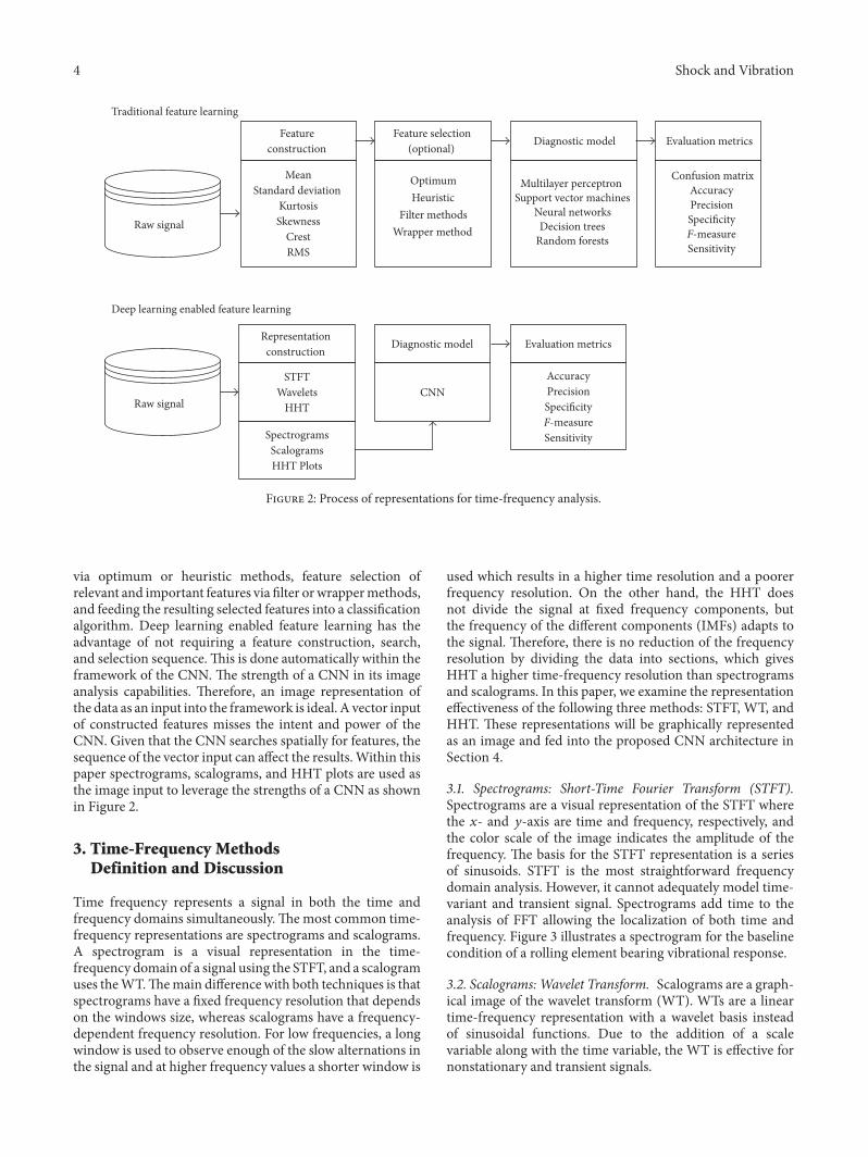
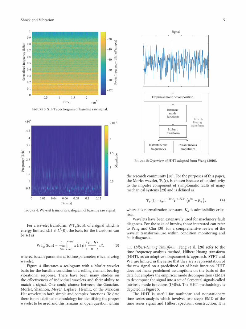
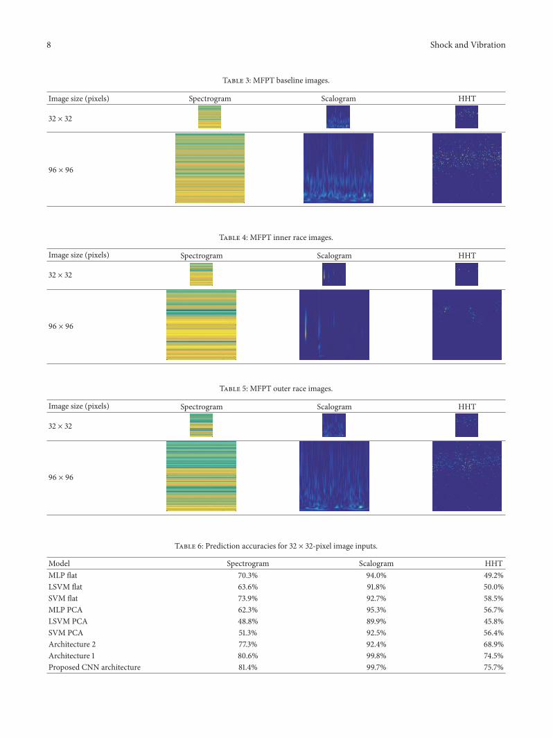
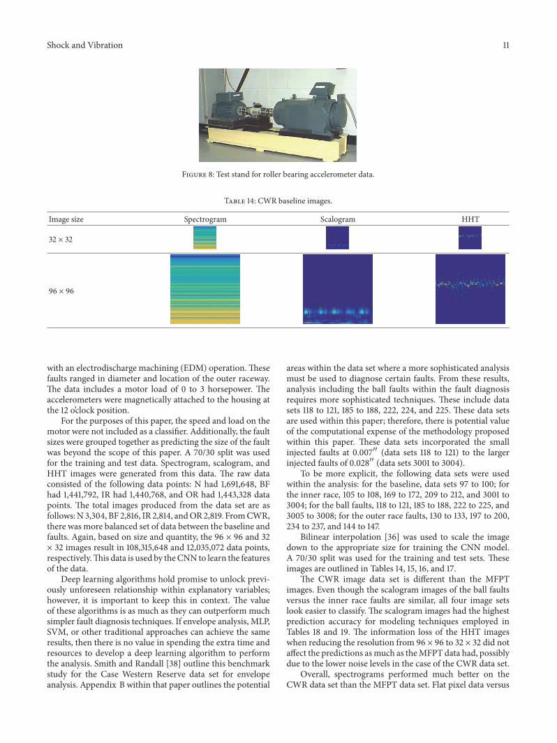
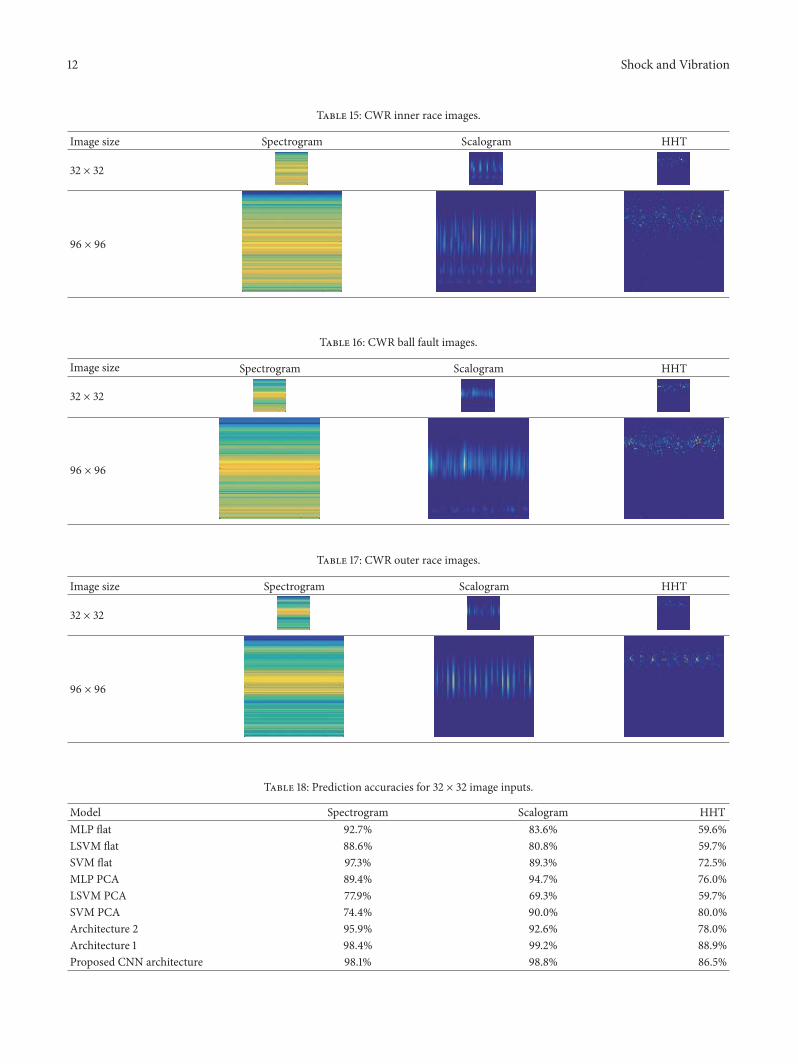
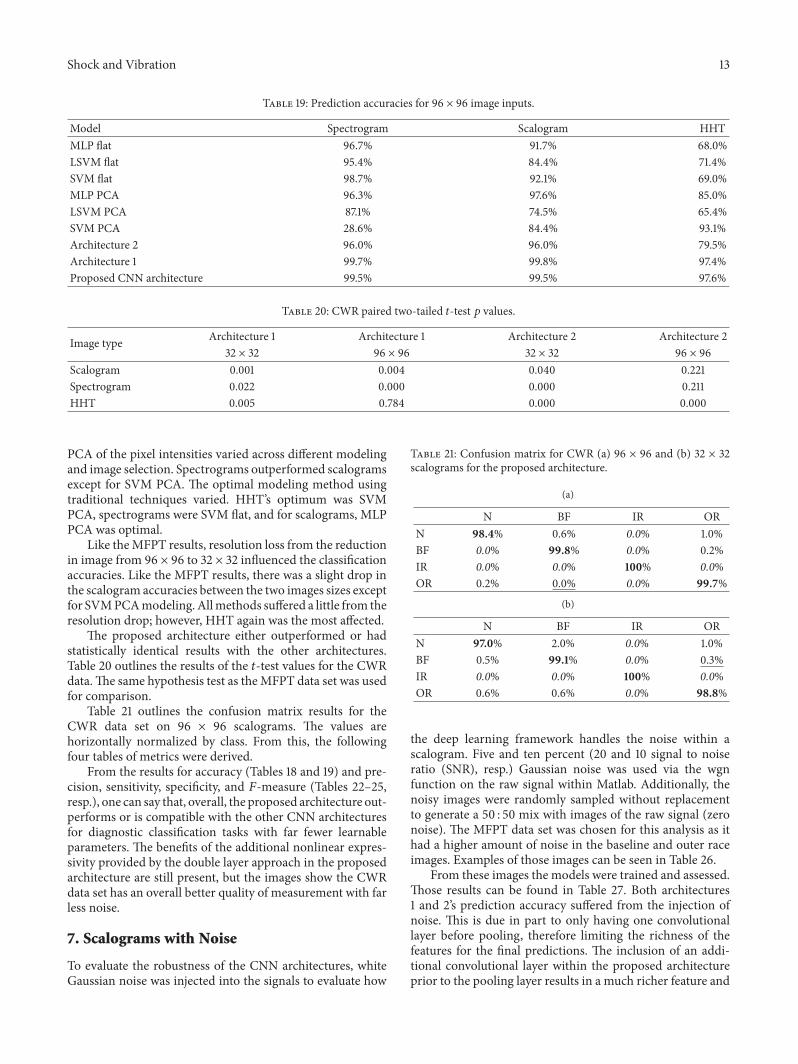
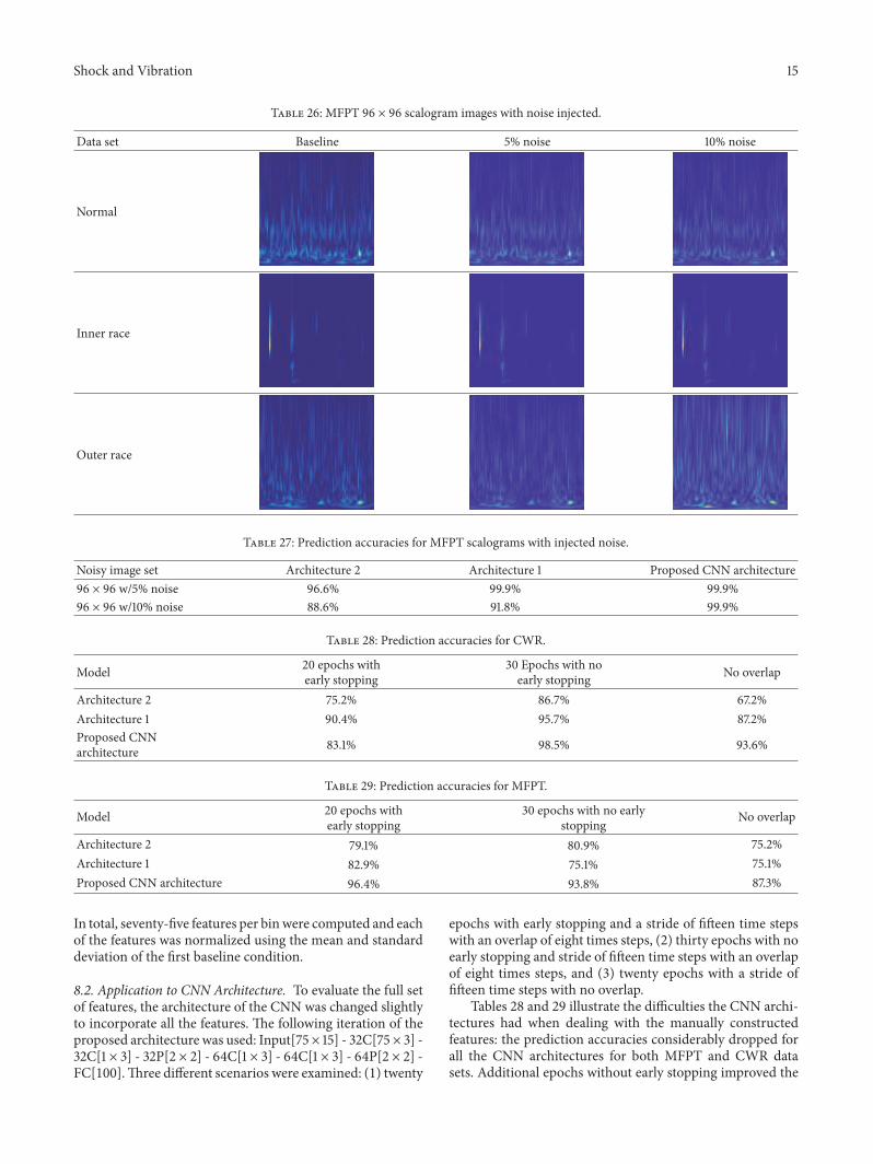
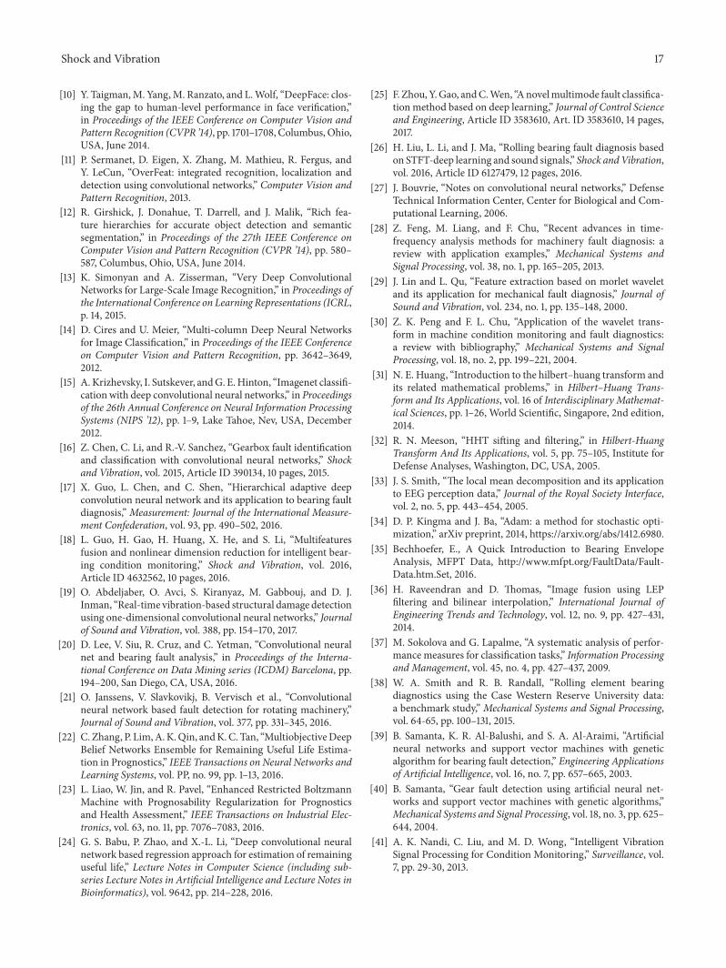