DEEP-LEARNING FEATURES, GRAPHS AND SCENEUNDERSTANDING

Thesis submitted in partial fulfillmentof the requirements for the degree of

Master of Science inComputer Science and Engineering by Research

by

ABHIJEET KUMAR201302197

abhijeet.kumar@research.iiit.ac.in

International Institute of Information TechnologyHyderabad - 500 032, INDIA

JANUARY 2020

Copyright c©ABHIJEET KUMAR, 2020

All Rights Reserved

International Institute of Information TechnologyHyderabad, India

CERTIFICATE

It is certified that the work contained in this thesis, titled “ DEEP-LEARNING FEATURES, GRAPHSAND SCENE UNDERSTANDING” by Abhijeet Kumar, has been carried out under my supervisionand is not submitted elsewhere for a degree.

Date Adviser: Dr. AVINASH SHARMACenter for Visual Information Technology,

Kohli Center on Intelligent Systems,IIIT Hyderabad

To Time

Acknowledgments

As I submit my thesis, I extend my gratitude to all those people who helped me in successfullycompleting this journey.

Foremost my deepest gratitude to Prof. Avinash Sharma and Prof. Madhav Krishna for their constantsupport and encouragement to explore and chart my own research path. Im really fond of my stints as aTA under Prof. Naresh Manwani and Prof. Ravi Kiran. I would also like to extend my sincerest thanks toProf. Vineet Gandhi and Prof. Vineet Balasubramian with whom my collaborations did not bore fruit.

I would also show my gratitude to the CVIT ecosystems, through which I came to have multipletechnical/non-technical discussions with wide background of students in PhD/MS/Honors and alsodeveloped an understanding of the vast variety of problems begin attempted at the centre. The names inthis list are too many and it is almost impossible to enumerate all of them.

I will also like to thank my parents and my brother whose support has been always immense in all myadventures in life. I would like to thanks my friends ( especially Rohit, Noor, Anurag, Yash, Anchal, Abb-hinav, Govinda and Anuj) at IIIT-Hyderabad who have provided motivation, philosophical discussions,Dullah Talks etc. I also appreciate the tolerant nature of my co-authors (Gunshi Gupta and Anjali Shenoy).

I will always look back to enjoy the fond memories I have of this institute.

v

Abstract

Scene Understanding has been a major aspiration of computer vision from its early days. Its rootlies in enabling the computer/robot/machine to understand, interpret and manipulate visual data, insimilarity to what an average human eye does in front of a natural/artificial localized location/scene.This ennoblement of the machine have a widespread impact ranging from Surveillance, Aerial Imaging,Autonomous Navigation, Smart Cities and thus scene understanding have remained as an active area ofresearch in the last decade.

In the last decade, the scope of problems in the scene understanding community has broadened fromImage Annotation, Image Captioning, Image Segmentation to Object Detection, Dense Image Captioning,Instance Segmentation etc. Advanced problems like Autonomous Navigation, Panoptic Segmentation,Video Summarization, Multi-Person Tracking in Crowded Scenes have also surfaced in this arena and arebeing vigorously attempted. Deep Learning has played a major role in this advancement/development.The performance metrics in some of these tasks have more than tripled in the last decade itself but thesetasks remain far from solved. Success originating from deep learning can be attributed to the learnedfeatures. In simple words, features learned from a Convolutional Neural Network trained for annotationare in general far more suited for captioning then a non-deep learning method trained for captioning.

Taking cue from this particular deep learning trend, we dived into the domain of scene understandingwith the focus on utilization of prelearned-features from other similar domains. We focus on two tasks inparticular: Automatic (multi-label)Image Annotation and (Road)Intersection Recognition. Automaticimage annotation is one of the earliest problems in scene understanding and refers to the task of assigning(multiple) labels to an image based on its content. Whereas intersection recognition is the outcome ofthe new era of problems in scene understanding and it refers to the task of identifying an intersectionfrom varied viewpoints in varied weather and lighting conditions. We focused on this significantly variedtask approach to broaden the scope and generalizing capability of the results we compute. Both imageannotation and intersection recognition pose some common challenges such as occlusion, perspectivevariations, distortions etc.

While focusing on the image annotation task we further narrowed our domain by focusing on graphbased methods. We again chose two different paradigms: a multiple kernel learning based non-deeplearning approach and a deep-learning based approach, with a focus on bringing out contrast again.Through quantitative and qualitative results we show slightly boosted performance from the abovementioned paradigms. The intersection recognition task is relatively new in the field. Most of thework in field focuses on Places Recognition which utilized only single images. We focus on temporalinformation i.e. the traversal of the intersection/places as seen from a camera mounted on a vehicle.

vi

vii

Through experiments we show a performance boost in intersection recognition from the inclusion oftemporal information.

Contents

Chapter Page

1 Introduction . . . . . . . . . . . . . . . . . . . . . . . . . . . . . . . . . . . . . . . . . . 11.1 Multi-Label Image Annotation . . . . . . . . . . . . . . . . . . . . . . . . . . . . . . 21.2 Intersection/Junction Recognition . . . . . . . . . . . . . . . . . . . . . . . . . . . . 21.3 Associated Challenges . . . . . . . . . . . . . . . . . . . . . . . . . . . . . . . . . . 31.4 Our Contributions . . . . . . . . . . . . . . . . . . . . . . . . . . . . . . . . . . . . . . 71.5 Thesis Overview . . . . . . . . . . . . . . . . . . . . . . . . . . . . . . . . . . . . . . 7

2 Related Works . . . . . . . . . . . . . . . . . . . . . . . . . . . . . . . . . . . . . . . . . 82.1 Image Annotation . . . . . . . . . . . . . . . . . . . . . . . . . . . . . . . . . . . . . 8

2.1.1 Generative, Discriminative and Hybrid Models . . . . . . . . . . . . . . . . . 82.1.2 Nearest Neighbor Approaches . . . . . . . . . . . . . . . . . . . . . . . . . . 82.1.3 Graph Based Models . . . . . . . . . . . . . . . . . . . . . . . . . . . . . . . 92.1.4 Deep Learning Based Methods . . . . . . . . . . . . . . . . . . . . . . . . . . 92.1.5 Graph Based Deep Learning Models . . . . . . . . . . . . . . . . . . . . . . . 10

2.2 Intersection Recognition . . . . . . . . . . . . . . . . . . . . . . . . . . . . . . . . . 102.3 Graphs Deep Learning . . . . . . . . . . . . . . . . . . . . . . . . . . . . . . . . . . . 11

2.3.1 Spectral Graph Theory . . . . . . . . . . . . . . . . . . . . . . . . . . . . . . 132.3.2 Graph Signal Processing . . . . . . . . . . . . . . . . . . . . . . . . . . . . . 13

3 Image Annotations with Multiple Kernel Learning(MKL) . . . . . . . . . . . . . . . . . . . 163.0.1 Our Contributions . . . . . . . . . . . . . . . . . . . . . . . . . . . . . . . . . 17

3.1 Proposed Approach . . . . . . . . . . . . . . . . . . . . . . . . . . . . . . . . . . . . . 173.1.1 Nearest Neighbors Search . . . . . . . . . . . . . . . . . . . . . . . . . . . . 183.1.2 Local Graph Construction . . . . . . . . . . . . . . . . . . . . . . . . . . . . 183.1.3 LLD Feature Construction, Clustering and Mapping . . . . . . . . . . . . . . 193.1.4 Diffusion Kernel . . . . . . . . . . . . . . . . . . . . . . . . . . . . . . . . . 19

3.1.4.1 Diffusion Scale Normalization. . . . . . . . . . . . . . . . . . . . . 193.1.5 MKL Formulation for Label Diffusion . . . . . . . . . . . . . . . . . . . . . . 203.1.6 Label Diffusion & Prediction . . . . . . . . . . . . . . . . . . . . . . . . . . . . 21

3.2 Datasets . . . . . . . . . . . . . . . . . . . . . . . . . . . . . . . . . . . . . . . . . . 223.2.1 PascalVOC-2007 . . . . . . . . . . . . . . . . . . . . . . . . . . . . . . . . . 223.2.2 MIRFlickr-25k . . . . . . . . . . . . . . . . . . . . . . . . . . . . . . . . . . 23

3.3 Experiments & Results . . . . . . . . . . . . . . . . . . . . . . . . . . . . . . . . . . 233.3.1 Features and Evaluation Method . . . . . . . . . . . . . . . . . . . . . . . . . 233.3.2 Experiments . . . . . . . . . . . . . . . . . . . . . . . . . . . . . . . . . . . 23

viii

CONTENTS ix

3.3.3 Results and Discussions . . . . . . . . . . . . . . . . . . . . . . . . . . . . . 24

4 Image Annotations with Graph Deep Learning . . . . . . . . . . . . . . . . . . . . . . . . . 294.0.1 Our Contributions . . . . . . . . . . . . . . . . . . . . . . . . . . . . . . . . 30

4.1 Background . . . . . . . . . . . . . . . . . . . . . . . . . . . . . . . . . . . . . . . . 304.2 Proposed Approach . . . . . . . . . . . . . . . . . . . . . . . . . . . . . . . . . . . . . 31

4.2.1 Label Modelling . . . . . . . . . . . . . . . . . . . . . . . . . . . . . . . . . . 314.2.1.1 Knowledge Graph . . . . . . . . . . . . . . . . . . . . . . . . . . . . 314.2.1.2 Graph Signals . . . . . . . . . . . . . . . . . . . . . . . . . . . . . 33

4.2.2 Image Representation . . . . . . . . . . . . . . . . . . . . . . . . . . . . . . . 334.2.3 Joint Space . . . . . . . . . . . . . . . . . . . . . . . . . . . . . . . . . . . . 334.2.4 Network Architecture . . . . . . . . . . . . . . . . . . . . . . . . . . . . . . . 334.2.5 Training and Network Parameters . . . . . . . . . . . . . . . . . . . . . . . . 33

4.3 Dataset . . . . . . . . . . . . . . . . . . . . . . . . . . . . . . . . . . . . . . . . . . 344.3.1 MSCOCO . . . . . . . . . . . . . . . . . . . . . . . . . . . . . . . . . . . . . 34

4.4 Experiments . . . . . . . . . . . . . . . . . . . . . . . . . . . . . . . . . . . . . . . . 354.4.1 Evaluation Metrics . . . . . . . . . . . . . . . . . . . . . . . . . . . . . . . . 354.4.2 Baselines . . . . . . . . . . . . . . . . . . . . . . . . . . . . . . . . . . . . . 35

4.5 Results and Discussions . . . . . . . . . . . . . . . . . . . . . . . . . . . . . . . . . . 354.5.1 Quantitative Evaluation . . . . . . . . . . . . . . . . . . . . . . . . . . . . . . 35

4.5.1.1 Knowledge Graphs and Input Signals . . . . . . . . . . . . . . . . . 354.5.1.2 Comparison with other methods . . . . . . . . . . . . . . . . . . . . 36

4.5.2 Qualitative Results . . . . . . . . . . . . . . . . . . . . . . . . . . . . . . . . . 37

5 View Invariant Trajectory Mapping for Autonomous Driving . . . . . . . . . . . . . . . . . 385.0.1 Contributions . . . . . . . . . . . . . . . . . . . . . . . . . . . . . . . . . . . 38

5.1 Proposed Approach . . . . . . . . . . . . . . . . . . . . . . . . . . . . . . . . . . . . 395.1.1 Convolutional Neural Networks (CNNs) . . . . . . . . . . . . . . . . . . . . . 405.1.2 Bidirectional LSTM . . . . . . . . . . . . . . . . . . . . . . . . . . . . . . . 405.1.3 Siamese Network . . . . . . . . . . . . . . . . . . . . . . . . . . . . . . . . . 405.1.4 Training and Network Parameters . . . . . . . . . . . . . . . . . . . . . . . . . 41

5.2 Experiments & Results . . . . . . . . . . . . . . . . . . . . . . . . . . . . . . . . . . . 415.2.1 Baselines / Evaluation Settings . . . . . . . . . . . . . . . . . . . . . . . . . . 425.2.2 Dataset Description . . . . . . . . . . . . . . . . . . . . . . . . . . . . . . . . 43

5.2.2.1 GTA . . . . . . . . . . . . . . . . . . . . . . . . . . . . . . . . . . 435.2.2.2 Mapillary . . . . . . . . . . . . . . . . . . . . . . . . . . . . . . . 44

5.2.3 Experimental Setup . . . . . . . . . . . . . . . . . . . . . . . . . . . . . . . . 455.2.4 Quantitative Results . . . . . . . . . . . . . . . . . . . . . . . . . . . . . . . 455.2.5 Qualitative Results . . . . . . . . . . . . . . . . . . . . . . . . . . . . . . . . 46

6 Conclusion . . . . . . . . . . . . . . . . . . . . . . . . . . . . . . . . . . . . . . . . . . . 51

Bibliography . . . . . . . . . . . . . . . . . . . . . . . . . . . . . . . . . . . . . . . . . . . . 53

List of Figures

Figure Page

1.1 Multi-label image annotation problem setup . . . . . . . . . . . . . . . . . . . . . . . 31.2 Intersection recognition problem setup: Given two videos consisting of road traver-

sal(in red and green) of intersection, identify if they belong to the same geographicalplace/location. . . . . . . . . . . . . . . . . . . . . . . . . . . . . . . . . . . . . . . . 4

1.3 Challenges: (a) Illumination Changes, (b) Occlusion, (c) Dynamic Background. Imagesare taken from Mapillary and Google Images. . . . . . . . . . . . . . . . . . . . . . . 5

1.4 Challenges: (a) Weather Changes, (b) Structural Changes . . . . . . . . . . . . . . . . 6

3.1 Pipeline showing flow of testing & training phase . . . . . . . . . . . . . . . . . . . . 183.2 Diffusion scale normalization on a sample graph of 56 nodes. In this case we use the

12th (= 0.2 ∗ |56|) eigenvalue and θ = 0.26 for computing the scale normalized t value.In general a set of θ values will be chosen for defining bank of diffusion kernels . . . . 20

3.3 Distribution of label frequency in MIRFlickr-25k and PascalVOC-2007 test images. . 253.4 Qualitative results for label prediction on MIRFlickr-25k dataset. Row1: images with

frequent labels(male, people); Row2: images with no ground truth label given; Row3:images with rare labels(baby, potrait). Green: Labels present in ground-truth and ourmodel’s predictions (true positives) , Blue: Incorrect predictions by the model and Red:Labels are not present in ground truth but are semantically meaningful. Red and bluelabels combined form False Positives . . . . . . . . . . . . . . . . . . . . . . . . . . . . 27

3.5 Qualitative results for label prediction on PascalVOC-2007 dataset. Row1: images withfrequent labels(person, car); Row2: images with rare labels(boat, cow). Green: Labelspresent in ground-truth and our model’s predictions (true positives) , Blue: Incorrectpredictions by the model . . . . . . . . . . . . . . . . . . . . . . . . . . . . . . . . . 28

4.1 Proposed approach: Given an input image, its representation is computed by passing itthrough VGG16(fc7 layer) network with pretrained weights. On other hand Faster-RCNNdetections are passed as input signals to graph which undergoes through 2 stages of graphconvolution and pooling layers(as defined in [21]. Later both the above representationsare concatenated and passed through a fully connected neural net before final prediction.Note that colors denote activated(non-zero) signals and the width of the edges denotedifferent edge-weights. Notice that one of node is is inactive after 1st convolution layer.This depicts that the diffusion of the signals is limited in the framework due to the choiceof the parameter K(=2 here) in Equation 4.3 (Best seen in color) . . . . . . . . . . . . 32

x

LIST OF FIGURES xi

4.2 Qualitative results for label prediction on MSCOCO dataset. 4 randomly selected samplesand their predictions and ground truth labels(color coded). Green: Labels present inground-truth and our model’s predictions (true positives), Blue: Incorrect predictions bythe model (false positives). Red: Missed Predictions (false negatives) (Best seen in color) 37

5.1 Proposed model is shown with video pairs as input and binary-classification as theoutput. Features from pretrained CNN network are fed into bidirectional LSTM withshared-weights as shown with hidden units in green (unfolded in time). . . . . . . . . 39

5.2 Data Visualization: Random snapshots from GTA environment [2] (Row 1) and Map-illary [4] (Row 2). Images show different weather and day/night conditions as wellas various outdoor scenes for urban scenarios. The game-environment snapshots lookvisibly similar to that of real world images and have significantly higher variations inweather and lighting. (Best seen in color) . . . . . . . . . . . . . . . . . . . . . . . . 42

5.3 Three correctly classified samples from Mapillary. Each sample depicts unique trajectory-relation and view-overlap between trajectories as shown in the intersection-map (bottom-most row) which represents the top-view of the intersection. We color encode the visuallyperceptible common structures (cyan, green, red, brown) in the Video pairs. Video pair 2and Video pair 3 show examples where trajectory direction and view overlap. Video pair1 depict cases when the overlap in trajectories and/or the view is minimal. (Best seen incolor) . . . . . . . . . . . . . . . . . . . . . . . . . . . . . . . . . . . . . . . . . . . . 47

5.4 Two correctly classified samples from GTA. Video pair 2 show examples where trajectorydirection and view overlap. Video pair 1 depict case when the overlap in trajectoriesand/or the view is minimal. (Best seen in color) . . . . . . . . . . . . . . . . . . . . . 48

5.5 Failure Cases: Three wrong predictions by the network. Video pair 1 consist of trajec-tories from different intersections but is predicted as the same intersection. In contrast,video pair 2, 3 consist of trajectories from the same-intersection but are predicted asdifferent intersection . . . . . . . . . . . . . . . . . . . . . . . . . . . . . . . . . . . 48

5.6 Failure Cases(False Positives): Two wrong predictions by the network. Video pair 1and 2 consists of trajectories from different intersections but is predicted as the sameintersection. Both the trajectories in Video-Pair 1 capture the side-view of the roadtraversal which adds to complexity of intersection recognition. Video-Pair 2 is in facta true failure case and we believe sch errors are acceptable due to the sufficient visualsimilarity in the videos. . . . . . . . . . . . . . . . . . . . . . . . . . . . . . . . . . . 49

5.7 Failure Cases(False Negatives): Two wrong predictions by the network. These Videopairs belonged to the same intersection but were predicted as different by the network. 50

List of Tables

Table Page

3.1 Dataset details: Row 2-4 contain basic dataset information, Row 5-6 denote the statics inthe order- median, mean and max. . . . . . . . . . . . . . . . . . . . . . . . . . . . . 22

3.2 Comparison of popular methods on different evaluation metrics for MIRFlickr-25kDataset for r = 5 . . . . . . . . . . . . . . . . . . . . . . . . . . . . . . . . . . . . . 24

3.3 Label specific (Average Precision in %) for all labels, mAP, P@r, R@r and F1@r withr = 2 on PascalVOC-2007 dataset. . . . . . . . . . . . . . . . . . . . . . . . . . . . . 25

4.1 Ablation Study: Performance variation due to different knowledge graph and graphsignal in our model. In row-5, the graph input signal is not binarized after thresholding. 35

4.2 Comparison of popular methods on different evaluation metrics for MSCOCO dataset . 36

5.1 Number of video pairs in training, testing and the validation set for the different experi-mental scenarios . . . . . . . . . . . . . . . . . . . . . . . . . . . . . . . . . . . . . . 43

5.2 Accuracy, Precision, Recall and F1 of our method on different datasets for the differentexperimental scenarios . . . . . . . . . . . . . . . . . . . . . . . . . . . . . . . . . . 44

5.3 X-View results on Mapillary: F1-scores at different experimental threshold (querysequence length: 15) . . . . . . . . . . . . . . . . . . . . . . . . . . . . . . . . . . . 46

xii

Chapter 1

Introduction

Scene understanding has been an important goal of computer vision systems - to enable machinesidentify, interpret and manipulate objects, surfaces and their interactions in images and videos andinterpret relationships between them. Tackling/Attempting problems from the domains of scene un-derstanding entails compatible data. For example learning to identify faces requires a corpus of facedataset. The widespread outburst of digital data, enabled by ever speeding network services, increasingsmart electronic devices(mobiles, tablets) and fast-paced lifestyle, has led to a steep rise in data-driventechnologies and has opened up a scope for vast number of complex problems. A decade ago problemsin scene understanding consisted of image-captioning, image annotation, object detection etc while thecurrent focus is on problems 3D reconstruction from 2D images, panoptic segmentation, multi-persontracking in crowds, very long video summarization. Currently, scene understanding is in the core ofmany imminent successes of modern technology - autonomous driving, human-machine interaction,remote sensing, among several others. Deep Learning, a subset of machine learning, has been shown tobenefit from huge amounts of data and has been an active area of research. Currently models based ondeep-learning forms state of the art for vast array of problems.

Our focus in this thesis derives both from the paradigm shift in the complexity of the problems inthe domain of scene understanding and the success of deep learning(specifically deep learning features).To limit the scope of our work, we select two problems from scene understanding (i) Multi-label imageannotation and (ii) Intersection recognition in road junctions. Multi-label image annotation can becategorized into a traditional scene understanding problem, whereas intersection recognition can becategorized into modern scene understanding problems. Our work in the image annotation domainfocuses on graph based learning. Here we have focused on two specific directions, Chapter 3 focuses ontraditional(non-deep learning) graph based approach whereas Chapter 4 focuses on graph deep learningbased approach. We also utilize deep learning features in our work. Specifically, we use pre-traineddeep learning models to extract representations for images which we use later in our models. Apart fromdeep-learning features Chapters 4 and 5 also utilizes state of the art deep learning architectures.

Now we brief the organization of this chapter. We first detail the motivations and problem definitionsfor the task of multi-label image annotation and intersection recognition. We then discuss the associated

1

challenges in these tasks and lay down our contribution in this thesis. We finally provide an overview ofthe remainder of the chapters in this thesis.

1.1 Multi-Label Image Annotation

The goal of the multi-label image annotation task is to assign all semantically meaningful labels1

to an image. Multi-label image annotation has applications in nearly every application domain ofcomputer vision ranging from object detection, instance segmentation, captioning, robotics, remotesensing, autonomous driving, surveillance, medical imaging etc. Multi-label image annotation is one ofthe keystone of scene understanding.

The term “semantically meaningful” could lead to a very large number of labels for any image. Henceto limit this set of labels, a label-set or dictionary of labels/tags/words to chose from is also provided.Tagging all the relevant words from this label-set/dictionary is the practical scenario of the task at hand.Its easily observable the the visual content of an image captures a wide variety of semantics at multiplelevels of granularity. Figure 1.1 shows an example from MSCOCO dataset on the left and a dictionaryof words on the right(also indicated is their presence/absence in the image).

Multi-label image annotation is a variant of single-label image annotation (commonly known as ImageAnnotation) where each image is tagged with just one relevant label from a dictionary set. It is imperativeto follow that single-label image annotation closely resembles to multi-label image annotation but simpleextensions to single-label task do not perform as good on the multi-label task. This argument is validatedfrom observing the current state of the arts in two tasks:- while single-label image annotation is close tobeing solved (a top-5 accuracy of 98% on the Image-Net dataset is already achieved), multi-label imageannotation is far from solved(F1-score of around 75% on the MSCOCO dataset). We propose two graphbased models (one with a deep-learning setup and another without a deep learning setup) for this task.We elaborate on these models, their specific backgrounds, datasets used and results in Chapter 3 andChapter 4.

1.2 Intersection/Junction Recognition

A road intersection or a road junction 2 typically is a meeting point of three or four road segments. Inthis problem, we focus on recognizing weather two given videos consist of same geographical locationwhile only using a monocular camera mounted on the top of a vehicle. A road intersection is hard torecognize as the approach to it could be from any of the 3 or 4 road segments its composed of, each ofwhich have a different view(backgrounds are completely different) of the intersection. Figure 1.2 depictsthe scenario of an intersection and two traversals(in red and green) of this intersection.

1We refer the words labels and tag interchangeably2We refer the words junction and intersection interchangeably

2

(a) An image from MSCOCO dataset

PersonGrassFootball

CloudsCake

Donut

(b) An example of a dictionaryof words. The tick/wrong marksindicate weather the label/tag ispresent in the image on the left

Figure 1.1: Multi-label image annotation problem setup

Recognizing an intersection from a different approach sequence or a sequence of viewpoints differentfrom those seen before can be pivotal in various applications that include autonomous driving, driverassistance systems, loop detection for SLAM including multi-robot and multi-session SLAM frameworks.Intersection recognition from disparate video streams or image sequences is an extremely challengingproblem that stems from the large variations in viewpoint, weather and appearance across traversals.Complexity also emanates from varying levels of traffic and chaos at a junction, as well as due to changinglevels of occlusion, illumination between two video sequences of a specific junction. Lack of annotateddatasets on intersections also poses a challenge.

Intersections being critical points in road based navigation, are likely to be points of crossover betweentrajectories of multiple agents/cars. Owing to their four-way structure, imagery captured in differenttraversals of junctions depicts very different views and alignment of common landmarks unlike what isobserved in place recognition datasets(e.g., [68]). If agents can recognize a previously visited place betterin such tricky scenarios, they are endowed with better localization capability. Intersection recognitionalso closely follows intersection detection [10], wherein the immediate question to answer upon detectingan intersection is if the detected intersection is the same as one seen previously. We proposed a novelLSTM based Siamese style deep network model for this problem while showing competitive results onreal and synthetic datasets. We elaborate on this model, datasets for this task and results in Chapter 5.

1.3 Associated Challenges

A wide variety of challenges can be associated with scene recognition. We provide a small brief ofsome of these challenges in this section.

3

Figure 1.2: Intersection recognition problem setup: Given two videos consisting of road traversal(in redand green) of intersection, identify if they belong to the same geographical place/location.

1. Illumination Changes: Lighting conditions in outdoor images vary drastically. They may rangefrom very high to very low foreground-background contrast. This might result in highlightingrandom objects in the scene. Indoor surroundings and illumination can be manipulated to make theobject of interest in focus with respect to the background. Illumination changes usually resultsin challenging problems for many computer vision applications such as recognition, tracking andmotion analysis. Figure 1.3a shows varying illumination conditions highlighting the backgroundor the foreground obscuring visibility.

2. Occlusion: In general, outdoor images have more than one object or the object interacts withelements of the surroundings. This leads to occlusion by some other object like a pole, buildingetc. These cases like partial or full occlusion create uncertainty in determining the location ofobject which are not visible. Apart from the above mentioned occlusions which were caused by anoutside entity (whether living or non-living object), the object of interest can occlude itself, whichis termed as self occlusion. Figure 1.3b shows such examples of occlusion.

3. Dataset Bias: Each image can be tagged with multiple labels from the given dictionary but ingeneral some labels appear more frequently then others. In-fact the occurrence pattern of labelsfollows the long-tail curve. This implies that a few labels appear most of time and the rest occursonly a few times in the presented dataset. This includes a heavy bias in the dataset which needs tocontrolled in order to make recognition unbiased.

4

(a)

(b) (c)

Figure 1.3: Challenges: (a) Illumination Changes, (b) Occlusion, (c) Dynamic Background. Images aretaken from Mapillary and Google Images.

4. Incomplete Labelling: Creation of a dataset involves manual labelling of images. This tasks isdone by human annotators who are not good at these mundane tasks. This may result in imagesnot being tagged with all the potential labels. Figure 1.1 shows such an example where the imagecan also be labelled with grass. To curb these error, multiple annotators label the images in morerecent datasets.

5. Dynamic Background: Some parts of the scene may contain movement (a fountain, movementof other objects, the swaying of tree branches, water waves etc.), but should be regarded as back-ground, according to their relevance. Such movement can be periodical or irregular (e.g., trafficlights, waving trees). Handling such background dynamics is a challenging task. Figure 1.3cshows examples of dynamic background having water waves from the fountain.

6. Weather Change: Outdoor scenes may look very different during different seasons/weathers.While a foggy/rainy day may hinder capturing the background while a sunny day will have bettercontrast and shinier objects. Figure 1.4 (a) shows an image of on a rainy and a summer day.

5

7. Object Speed: The speed of the moving object plays an important role in its detection. Intermittentmotions of objects cause ghosting artifacts in the detected motion, i.e., objects move, then stopfor a short while, after which they start moving again. There may be situations in a video, wherethe still objects suddenly start moving, e.g., a parked vehicle driving away, and also abandonedobjects.

8. Shape and Structural changes: A single object can have many different structural possibilitieswhich makes a direct modelling of an object in general near impossible. Similarly, non-rigidobjects can change shape when forces are applied on them. An example of this could be the poseof a human when he/she is moving. Figure 1.4b shows an example images of chair which arestructurally different.

9. View Variations: Different camera positions may capture the same geographical location but thecorresponding images are likely to different. One such possibility arises when an image capturesthe front of a building while the other captures the back-view of the same building. In such casebackgrounds of the two images may overlap partially or not overlap at all. Figure 1.4a shows anexample where the Eiffel Tower is captured from two different viewpoints.

(a)

(b)

Figure 1.4: Challenges: (a) Weather Changes, (b) Structural Changes

6

1.4 Our Contributions

The main contribution of this thesis are:

1. Multi-label image annotation We introduced the notion of neighborhood-types and proposed anew label histogram characterization of image-neighborhoods. The notion of neighborhood-typesis based on hypothesis that similar images in content/feature space should also have overlappingneighborhoods. Building upon this we used diffusion as label transfer mechanism to associate tagsand derived a closed from solution.We also explored Graph Convolution Neural Networks for multi-label image annotation wherewe propose a graph based deep-learning solution for the problem of multi-label classification.Through extensive experimentation of our architecture, we explore the effects of graph formationand the input signals on the performance.

2. Intersection/Junction recognition We proposed a novel stacked deep network ensemble architec-ture that combines state-of-the-art CNN, bidirectional LSTM and Siamese style distance functionlearning for the task of view-invariant intersection recognition in videos. We have collectedannotated data of around 2000 videos from GTA gaming platform and Mapillary consisting ofvaried weather conditions and varied viewpoints.

1.5 Thesis Overview

Now we provide the organizational scheme of the upcoming chapters in this thesis. The outline of thefollowing chapters is:

• Chapter 2 provides the literature survey for image-annotation, intersection recognition and deeplearning in graphs.

• Chapter 3 details out our approach for image annotation via diffusion combined with MultipleKernel Learning (MKL) model.

• Chapter 4 describes our approach, experiments and results using graph based deep learning modelfor image annotation.

• Chapter 5 dives into the problem of intersection recognition.

• Finally chapter 6 summarizes the main contributions of the thesis.

Furthermore, each of Chapter 3 and Chapter 4 is broken down into (i) Motivation, Brief and Contribu-tions (ii) Proposed Approach (iii) Dataset (iv) Experiments and (v) Results and Discussions.

7

Chapter 2

Related Works

2.1 Image Annotation

Over the last two decades, a plethora of methods have appeared in this area. We brief about a lot ofthese methods while our focus is on most relevant, popular and recent methods. We try to categorize theprevious works into 5 categories based on the underlying model’s ideology.

2.1.1 Generative, Discriminative and Hybrid Models

Sahin et al. [25] model the problem from a machine translation perspective where a region is mappedto a label. Relevance Models [27, 53, 42] model the problem as joint probability distribution betweenimage features and labels. Multiple Bernoulli Relevance Model(MBRM) [27] proposed regular regionblocks for features and a multiple Bernoulli model using non-parametric kernel density estimate. TopicModels [8, 70, 25, 101] uses probabilistic method to represent the joint distribution of visual and textualfeatures by maximizing the generative data likelihood.

Xinag et al. [101] proposed a Markov Random Field model, which captured many previously proposedgenerative models, but had an expensive training step as it learnt an MRF per label. Discriminativemodels were proposed in [105, 33, 95, 28]. These methods learn label-specific models to classify animage belonging to the particular label. However they fail to capture label-to-label correlations. A hybridmodel was presented in [71] combining a generative [27] and discriminative (SVM) model aimed atimproving the number of labels recalled.

2.1.2 Nearest Neighbor Approaches

Though simple and highly intuitive, NN methods are among the best performing ones. [34] introducedmetric learning to fuse an array of low-level features. They used cross entropy loss in addition to weighted(based on distance or rank) label propagation. Recently, [96] defined a Bayesian approach with twopass kNN for addressing the class-imbalance challenge and subsequently used an extension of existingLMNN approach [100] as metric learning to fuse different feature sets. One major limitation of these

8

approaches is that they are global methods and heavily rely on metric learning construct, which makes itdifficult to scale them to large datasets.

Alternatively, a local variant of NN method proposed in [45] performs the Non-negative MatrixFactorization (NMF [54]) of features from images in a smaller neighborhood, which are made to follow aconsensus constraint. Here, the class-imbalance is dealt by means of weighting different feature matrices.However, this is purely a local approach and hence fails to capture the global structure of the latent space.

Recently, [92] and [96] report performance improvement over the NN methods by using cross modalembedding such as Canonical Correlation Analysis (CCA) or Kernel Canonical Correlation Analysis(KCCA). This is again an attempt to learn global common latent space. However selection of anappropriate kernel function and scalability of KCCA poses a major challenge in these methods.

2.1.3 Graph Based Models

A graph based transductive method for explicitly capturing label-to-label and image-to-image similari-ties was proposed in [97]. Recently, [73] proposed a hypergraph diffusion based transductive method andexploited multi-scale diffusion to address the class-imbalance problem. However, both these methodsare semi-supervised in the sense that they need access to all test data for prediction. Additionallythe hypergraph diffusion method is not scalable due to requirement of storage and computation ofeigen-decomposition of very large matrices.

2.1.4 Deep Learning Based Methods

Inspired by the recent success of deep neural net architectures in image classification [88, 86], differentapproaches involving deep nets have been tried for multi-label classification [40, 67, 99, 64, 102, 35,107, 15]. [40] modeled these relationship on a hierarchical model exploiting Long Short Term Memory(LSTM) by incorporating inter-level and intra-level label correlations which were parsed using WordNet.CNN-RNN [98] learns a joint image-to-label embedding and label co-occurrence model in an end-to-endway. Semantically Regularised CNN-RNN (S-CNN-RNN) [62] improves on the CNN-RNN model byusing a semantically regularized embedding layer as an interface between the CNN and RNN whichenables RNN to capture the relational model alone. [43] showed that the order of label predictionmattered while using RNN (or LSTM) for label modelling.

[44] proposed exploiting image metadata to generate neighbors of an image and blend visualinformation using neural-nets. Recent works in Deep nets capture label-to-label relationships moreexplicitly than before. Another recent work in [72] converted labels to a word2vec vector [67] andperformed label transfer using nearest neighbor methods in embedding space computed using CCA orKCCA. More recently visual attention models [35, 64, 99] have been on the rise too.

9

2.1.5 Graph Based Deep Learning Models

Recently deep-learning methods have been introduced in the context of graphs [24, 38, 80, 58]. GatedGraph Neural Network (GGNN) [58] is a LSTM variant for graphs which learns a propagation modelthat transfers information between nodes depending on the edge types. [66] introduced Graph SearchNeural Network (GSNN) which improves GGNN [58] by diminishing the computational issues. GSNNis able to reason about the concepts by capturing the information flow between nodes in the noisyknowledge-graphs. GSNN is different from our model in the propagation modeling in graphs. In Chapter4, we explicit model the label propagation with diffusion framework on graphs while GSNN learns thenetwork propagation parameters in the knowledge-graph.

Contemporary to this submission a recent graph based method [18] have been published. Similar toour work in Chapter 4, Chen et al. [18] models label patterns/co-relations utilizing graph convolutionnetworks, but they use the formulation from [48]. They also differ in the way they model Joint Space(refer Subsection 4.2.3) and their formulation of the knowledge graph matrix (refer Subsection 4.2.1.1).They utilize work-embedding as signals on nodes of the graph while we use Faster-RCNN [77] outputdetections as signals.

2.2 Intersection Recognition

In existing literature around robotic perception, there are limited efforts towards intersection detectionand recognition. Some of these use sensors other than cameras such as laser and virtual cylindricalscanners [108, 55].

Within the robotics community, loop detection methods have used diverse image recognition andretrieval techniques [32, 29, 5] that have not attempted to detect loops from very diverse viewpoints,though they perform admirably in the presence of weather changes [61] or under the duress of varyingtraffic [36]. In the vision community, CNN [87] features have been used to efficiently compare scenes orstructures which are viewed from varying distances, which give a zoom-in vis-a-vis zoom-out effect withminor changes in viewing angles.

Recently, a framework for detecting intersections from videos was proposed in [10]. They usedLSTM based architecture to observe the relative change in outdoor features to detect intersection.Nevertheless, their work did not focus on the recognition task. On the other hand, visual loop closuredetection techniques in the literature [6, 32, 29] mainly focused on image level comparison of scenes.These techniques try to find re-occurring scene during the driving session based on fast KD tree basedcomparison of image features. Although these methods achieve admirable accuracy for loop detectionthey cannot be improvised for view-invariant recognition over videos.

In recent years, gaming environments have been created and/or used for generating and annotatingdatasets. [78] used Grand Theft Auto V (GTA) gaming-engine to create large-scale pixel-accurate groundtruth data for training semantic segmentation systems. SYNTHIA [79] is a virtual world environmentwhich was created to automatically generate realistic synthetic images with pixel-level annotations for the

10

task of semantic segmentation. [78] and [79] show the added improvement in the real-world setting byusing synthetic-datasets for training deep-network models. CARLA [23] is another open-source simulatordeveloped to facilitate learning and testing of Autonomous Driving algorithms. GTA environment ismore visually realistic than SYNTHIA and CARLA environments.

Real-world datasets such as [69, 1] are designed with the idea of visual place recognition usingimages. These datasets are limited in the pathways covered and the number of intersections. Another realworld street-level imagery platform [4] consist of images and image-sequences with variability in thepathways and intersections and thus enables sequence learning for intersection recognition. Concurrentworks have used this platform to create Mapillary Vistas Dataset [74] which is a semantic segmentationdataset consisting of 25k images. We have used Mapillary dataset to showcase our result on real worldscenarios.

Recently [81] and [31] have attempted visual localization under drastic viewpoint changes. [81]needs various modes of data including: semantic segmentations, RGBD images and camera parameters.Its a computationally expensive pipeline focused on relocalization, involving 3D voxel grid constructionsof the entire previous traversal sequence and of the query sequence, followed by a matching and poseestimation procedure. Due to key differences in problem context and usage of multimodal inputs, weomit a quantitaive comparison with [81]. [31] proposes graph construction from semantically segmentedinput data with graph matching using random walk descriptors. We implement and compare againstthis method in a limited setup in our baseline experiments in Section 5.2.1. Specifically there has beenno prior effort towards recognizing intersections when approached from different road segments thatconstitute the intersection.

2.3 Graphs Deep Learning

In this section we first introduce a graph with notations. Then we provide the motivation for deeplearning in graphs. Then we mention a few existing works on networks on graph while paralelly followinga taxonomical categorization of graph networks. We then discuss in detail the spectral graph theory andgraph signal processing which forms a basis for understanding convolution operator in graphs. We thenmove exclusively to graph convolution networks and provide an overview.

A graph is defined as a set of elements and their pairwise connections. Mathematically, the set ofelements are defined as nodes or vertices and connections are known as edges. The set of nodes isdenoted as V = (v1, · · · , vn) and set of edges as E = {(vi, vj)|(vj ∼ vi) = wi,j ≥ 0}. An edge existsonly if two nodes have a relationship, wi,j is defined as the weight of the relationship between nodes vi,and vj . Graphs are categorized as non-euclidean data as the pairwise relationship may not necessarilybe an euclidean space distance of nodes. An edge can represent many sorts of relationships; similarity,dis-similarity, or a constraint. And weights can be used to define the magnitude of this relationship. Agraph can be represented by a matrix, called weighted adjacency matrix, W n×n whose (i, j)th entry wi,jis the similarity between vertices vi and vj , n being the number of nodes.

11

Traditional deep learning has majorly focused on the euclidean-space. In the deep learning era, one ofthe major works is CNN which utilizes the shift-invariance, local connectivity, and compositionality ofimage data. However, numerous applications, ranging from interactions and activities on social media,molecular activity and structure in drugs and program verification are based complex graph based data.Designing machine learning algorithms on such data is difficult as the graph domain is irregular i.e. eachgraph has a variable size of unordered nodes, each of which may be connected to a different set of othernodes. Furthermore these nodes are not independent of each other and are related via edges (whichcontains some linkage information). These properties makes it hard for defining a convolution operatorin this domain [12].

As per recent works the graph networks can be categorized under the following categories:

• Graph Recurrent Networks: These networks generalize the concept of recurrent networks in graphsbut instead of learning sequence outputs these networks outputs are node representations, graphrepresentations, etc which can be further used for classification or detection tasks. The core idea inthese networks are (i) node annotations (ii) information propagation model (which can use gatedequivalents of LSTM) and (iii) output models (which outputs the node/graph representations orselects specific nodes [80, 58].

• Graph Convolution Networks(GCN): These networks mimick the convolution operators fromtraditional data like images or grids to graph data. Specifically, they learn a function whichaggregates a node and its neighbors’ features [13, 21, 48, 56, 30, 75, 22, 16].

• Graph Attention Networks: Similar to GCN, these networks learn a function which aggregates anode and its neighbors features [93, 106]. The major difference with GCN is the use of parametricweights to implicitly capture the edge relationship/importance.

• Graph Auto-Encoders: To learn graph representations graph auto encoders employ an unsupervisedapproach. They consist of an encoder (underlying network could be GCN) and a decoder whichutilizes a link-decoder prediction [76, 104].

• Graph Generative Networks: Synthesizing complex chemical compounds with requisite physicaland chemical properties is a challenging task. Graph generative networks have shown promisein this highly specialized domain by alternatively generating nodes and edges and employingadversarial training [59, 11].

GCN can be further divided among two sub-categories: spectral-based and spatial-based. In spatialbased setup, GCN learns filters which aggregates features of a node and its neighbors. In spectral basedsetup, the learned filters are defined from the perspective of graph signal processing [12] which work in agraphs’ Fourier basis and manipulate/alter the magnitude of the frequencies. We describe this in detail inSubsection 2.3.2.

12

2.3.1 Spectral Graph Theory

For graphs the underlying non-euclidean topology is analyzed in terms of eigenvalue-eigenvectorspectrum of graph in the field of spectral graph theory [19]. Spectral analysis of a graph starts first byconstructing its Laplacian matrix Ln×n. If Dn×n is the degree matrix of the graph with its diagonalentries di,i representing the degree of node i, then L is defined as L = D −W .

Laplacian matrix represents the second-order derivative operator on the functions on a graph. In thisrespect it captures the topology of the graph and becomes a basis for defining all the operators over thegraph. Laplacian matrix provides a link between discrete graph representations and vectors in continuousEuclidean space. Mathematical operators defined in the continuous space are extended in the discretespace via the graph Laplacian matrix. Continuous-space kernels operate on vector valued functionsdefined by physical processes in that space. The discrete counterparts of these operators are the kernelsdefined as functions of the graph Laplacian. These kernels operate on functions or signals defined on thenodes of the graph.

One of the important properties of Laplacian matrix is that it is a positive semi-definite matrix, henceit is eigen-decomposable:

L = Un∗nΛn∗nUTn∗n (2.1)

where Λ is a diagonal matrix and U consists of orthonormal column vectors. Hence this can also bewritten as

L =n∑i

uiλiuTi (2.2)

where ui is a eigen(column)-vector and λi is the corresponding eigenvalue.An important random process over a graph is diffusion. These graph kernels operate on the real

valued functions f : V → R on the set V of the graph. Diffusion of a function on a graph captures thespatial extent of spread of the function with time. The kernel that captures the spatio-temporal extent ofdiffusion is the diffusion kernel H. The scale dependent diffusion kernel is:

H(t) = Ue−λtUT =n∑i

uie−λituTi (2.3)

The exponential function of the graph Laplacian is the kernel over the graph that represents the extentof diffusion of the function f at the diffusion scale t. Diffusion (or heat) kernel is uniquely defined at itsscale given the graph.

All these kernels can be principally put in another framework also. This framework extends theconcepts of signals and systems onto irregular domains such as graphs.

2.3.2 Graph Signal Processing

In the signal processing domain, a function is treated as a signal. If every node of the graph containsa signal(real-value), the combined signal over the entire graph is called a graph-signal s ∈ Rn. This

13

graph-signal forms a pattern over the graph-topology. The emerging field of graph-signal-processinganalyzes such graph-signals in terms of their components on defined harmonics based on the algebraicand spectral properties of graph-topologies [85].

We will first conceptualize the notion of frequency over a graph and the corresponding Fourier basisdefining the transform. For a 1-dimensional signal s(t) varying with time t, the Fourier transform is asfollows:

U(ω) =< s(t), ejωt >=

∫Rs(t)e−jωtdt, (2.4)

where ω is the angular frequency of the complex exponential basis signal and j =√−1. Every component

of the signal on a Fourier basis signal is the inner product between the two. Consider the eigenfunctionsof the 1-dimensional Laplacian operator:

∆(ejωt) =∂

∂t

( ∂∂t

(ejωt))

= jω∂

∂t(ejωt) = −ω2ejωt. (2.5)

These eigenfunctions are the Fourier basis signals with their corresponding eigenvalues as the square ofthe frequency. Thus the graph Fourier transform is defined as the expansion of a graph-signal in terms ofthe eigenvectors of graph-Laplacian:

si =< s, ui >=

n∑k=1

sku∗i (k)sn×1 = U>n×nsn×1(sinceLui = λiui) (2.6)

where U> representing the conjugate of the eigenvectors and Λ representing the square of the frequenciesof the graph-topology.

In the classical Fourier analysis the angular frequencies ω carry a specific meaning of frequency. Thesmaller the ω the slower the oscillation of the Fourier basis signal and vice-versa. And for ω = 0 thebasis signal takes a constant value. Similarly in the case of graphs, the graph Laplacian eigenvectorscorresponding to lower (higher) λi’s vary slowly (rapidly) on the graph, introducing the concept of graphharmonics. If there is a strong edge between two nodes, the dissimilarity between the values of theeigenvector on the two locations will increase with λ.

The inverse graph Fourier transform is also easily deducible:

s(t) =< U(ω), e−jωt >

s(t) = Us.(2.7)

In the above equation, the graph-signal u is represented as a linear combination of graph harmonics(columns of U ) where elements of s form the coefficients of linear combination which representcontribution of each component graph harmonic.

One of the most important aspects of signal processing is filtering of signals which have applicationsranging from noise-removal, compression, communication etc. Filtering operations in spatial domainrequire convolution operations. To define a convolution operation a notion of regular neighborhood ofeach point in the given space is necessary. Such a notion of neighborhood regular neighborhood could

14

be easily found out in euclidean spaces(or regular-grid spaces) such as temporal signal(audio), spatialsignal(image) or spatio-temporal(video). In these domain the convolution operator could be easily defineby sliding a filter of fixed size in a pre-defined method(example left to right and then top to bottom).Hence convolution can be simply computed as an integral/summation at each point with the center of thefilter colliding with the current point in space.

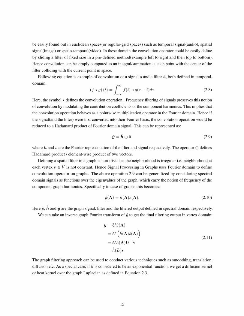
Following equation is example of convolution of a signal g and a filter h, both defined in temporal-domain.

(f ? g) (t) =

∫ ∞−∞

f(t) ∗ g(τ − t)dτ (2.8)

Here, the symbol ? defines the convolution operation.. Frequency filtering of signals preserves this notionof convolution by modulating the contribution coefficients of the component harmonics. This implies thatthe convolution operation behaves as a pointwise multiplication operator in the Fourier domain. Hence ifthe signal(and the filter) were first converted into their Fourier basis, the convolution operation would bereduced to a Hadamard product of Fourier domain signal. This can be represented as:

y = h� s. (2.9)

where h and s are the Fourier representation of the filter and signal respectively. The operator � definesHadamard product / element-wise product of two vectors.

Defining a spatial filter in a graph is non-trivial as the neighborhood is irregular i.e. neighborhood ateach vertex v ∈ V is not constant. Hence Signal Processing in Graphs uses Fourier domain to defineconvolution operator on graphs. The above operation 2.9 can be generalized by considering spectraldomain signals as functions over the eigenvalues of the graph, which carry the notion of frequency of thecomponent graph harmonics. Specifically in case of graphs this becomes:

y(Λ) = h(Λ)s(Λ). (2.10)

Here s, h and y are the graph signal, filter and the filtered output defined in spectral domain respectively.We can take an inverse graph Fourier transform of y to get the final filtering output in vertex domain:

y = U y(Λ)

= U(h(Λ)s(Λ)

)= U h(Λ)U>s

= h(L)s

(2.11)

The graph filtering approach can be used to conduct various techniques such as smoothing, translation,diffusion etc. As a special case, if h is considered to be an exponential function, we get a diffusion kernelor heat kernel over the graph Laplacian as defined in Equation 2.3.

15

Chapter 3

Image Annotations with Multiple Kernel Learning(MKL)

The task of automatic image annotation attempts to predict a set of semantic labels for an image. Ma-jority of the existing methods discover a common latent space that combines content and semantic imagesimilarity using the metric learning kind of global learning framework. This limits their applicability tolarge datasets. On the other hand, there are few methods which entirely focus on learning a local latentspace for every test image. However, they completely ignore the global structure of the data. In thiswork, we propose a novel image annotation method which attempts to combine best of both local andglobal learning methods. We introduce the notion of neighborhood-types based on the hypothesis thatsimilar images in content/feature space should also have overlapping neighborhoods. We also use graphdiffusion as a mechanism for label transfer.

The basic assumption in image annotation is that the visual content of an image captures a widevariety of semantics at different levels of granularity. Additionally, the label co-occurrence patterns alsomodel the semantic similarity between images. For example, the possibility of a car and a road tagappearing together in an image is highly likely as compared to a car and a plane. Therefore, existingmethods have tried to model label-to-label [65], image-to-image [34] and image-to-label [14] similaritiesor a combination of them [97, 63].

In context of image-to-image and image-to-label similarities Nearest Neighbor (NN) based approacheshave been largely successful and intuitive for image annotation. Recent methods either employ a global(metric) learning technique [96, 34] or a local query specific model [45] for addressing the class-imbalanceproblem. However, while the former suffers from the problem of scalability due to global metric learningbottleneck, the latter fails to capture the global latent structure of the data as it is too focused onquery specific neighborhood structure. An alternate approach in [73] addresses the class-imbalance byperforming scale-dependent label diffusion on global hypergraph in a transductive setup. However, theirmethod also suffers from the scalability issue (due to SVD decomposition of large dense matrices). Manyrecent deep learning methods also propose to learn end-to-end network for solving image annotationtask [72, 98, 62].

In this paper, we focus on bridging the gap between purely global and local modeling of the imageannotation task. The key hypothesis is that similar images in feature space also have similar labels,

16

hence two vicinal images in feature space should also have overlapping neighborhoods. Each of theseneighborhoods (corresponding to an image) can be statistically characterized by constructing the labelhistogram of all their associated images. We refer to these label histogram features as Local LabelDistribution (LLD) features. Thus, two similar images should have similar LLD feature representationwhich represent similarity in neighborhood. Hence we propose to learn a local label-transfer model foreach such neighborhood-type (cluster) separately. This characterization of images by neighborhood-typesalso inherently captures the global latent structure of data.

Subsequently, each local model is formulated as Multiple Kernel Learning (MKL) task, using afamily of multi-scale diffusion kernels. The MKL formulation minimizes the sum of squared errorbetween the ground truth labels (known for each training image) and the labels predicted with multi-scalediffusion over the associated local graph. Such diffusion is performed by linearly combining a set of scaledependent diffusion kernels. A closed form solution exists for obtaining the optimal kernel combinationcoefficients (parameters of local model). Thus, MKL parameters per neighborhood-type are learnt overthe training data. At test time, we construct and map the neighborhood structure of each query image toan existing neighborhood-type to retrieve the best parameter of local model. Finally, we construct thelocal graph for this query image and diffuse the label using these parameters for subsequent prediction.

3.0.1 Our Contributions

In this chapter we contribut in the following ways:

• We propose a new label histogram characterization (LLD features) of the image neighborhoodenabling us to discover the neighborhood-types in the dataset.

• We propose a MKL formulation as local learning model and derived a closed form solution forobtaining the model parameters.

• We propose a diffusion scale normalization procedure for effectively combining diffusion overmultiple graphs.

3.1 Proposed Approach

This section will provide a detailed description of each individual module in the proposed train and testphase flow pipeline depicted in Figure 3.1. Let Xtr = {x1, · · · ,xn} be the feature-vector representationof training set of images with corresponding known ground truth labels Ztr = {z1, · · · , zn}, where eachzi is a binary vector of size l denoting presence/absence of labels in the image xi ∈ Xtr.

17

Test Image

Nearest Neighbor Search

Construct Local Graph

LLD Feature Construction

LLD Mapping Label Diffusion Label Prediction

Train Images

Nearest Neighbor Search

Construct Local Graph

LLD Feature Construction

LLD Clustering

Solving for MKL Formulation

Compute Heat Kernels at

Normalized Scales

Compute Heat Kernels at

Normalized Scales

Train Phase flow-diagram

Test Phase flow-diagram

Parameters Learned per LLD cluster

Parameters Learned per LLD cluster

Figure 3.1: Pipeline showing flow of testing & training phase

3.1.1 Nearest Neighbors Search

This module performs feature space NN search for a given image in order to discover a group ofsimilar images. Instead of performing a global search, we opt for quantizing the feature space imagerepresentation by employing the paralleizable k-means clustering algorithm 1 on training data and findinga fixed g number of clusters in an offline manner. From all these clusters, we subsequently find thetop η closest cluster centers in feature space, then we perform the local NN search in those clustersby retrieving a fixed δ number of similar images from each of them. All such retrieved images formthe neighbourhood of a given image. We denote this set of nearest neighbor images obtained with thismethod for a given image x as N (x). Note that |N (x)| ≤ ηδ, as a cluster can have less than δ images.This naturally provides diversity and scalability over the exhaustive NN search.

3.1.2 Local Graph Construction

This module constructs an undirected weighted graph G(V,E,W) for an image x using the neighbor-hood N (x), where the input image and each of the selected images in N (x) images become nodes ofthe graph.

We construct a local graph by connecting each node to its k most similar nodes using an inverse eu-clidean distance similarity function over the corresponding image features. We use the standard Gaussiankernel over the feature space as the similarity function, i.e., Sim(x1, x2) = exp(−||x1, x2||l2/σ2) toassign weights to these edges.

Note that here |V | = ζ + 1 ≤ ηδ + 1 where |N (x)| = ζ

1https://github.com/serban/kmeans

18

3.1.3 LLD Feature Construction, Clustering and Mapping

This module first constructs an l-dimensional histogram feature F(x) for each image representing theLLD of a given image x, by taking the sum of ground truth labels of all the samples in N (x):

F(x) =∑

∀xi∈N (x)

zi. (3.1)

We employ parallelizable k-means clustering algorithm over the LLD features corresponding toall training images to get a fixed number of cluster-centers (c) which act as representatives of theneighborhood-types. To map an image to a neighborhood-type we just need to compute its closestneighborhood-type (cluster-centers) in this l-dimensional space. As discussed in Section 3, we discoverthe clusters in LLD space and learn a local model per cluster.

3.1.4 Diffusion Kernel

In this module we construct a family of diffusion kernels at different diffusion scales for a given localgraph computed in the previous module. In each weighted graph G(V,E,W), training images with labelsacts as heat sources that are diffused/propagated to all the other nodes in the graph where we aggregatethe information and subsequently use for prediction.

We have introduced graph laplacian in Subsection 2.3.1 (Mathematically in Equation 2.1). Diffusionkernel is a positive semi-definite, non-linear family of kernels and can be used for defining distancesover non-euclidean spaces and for multiscale-multilabel-diffusion in graphs. It has been used for multi-scale label diffusion over graphs [90], and a variety of other applications 3D Shape Matching [84]and Robotics graphSLAM [20] Subsequently, the scale dependent diffusion kernel matrix is definedas: H(t) = Ue−ΛtUT where t > 0 is the parameter of the diffusion. Every entry H(i, j, t) of thediffusion kernel can be interpreted as the amount of heat diffused from node vj to node vi at scale t whileconsidering vj as a point heat source of unit magnitude. We use the diffusion kernel matrix at m differentscales to diffuse each label. This is different from [73] as we use multiple scales for all labels rather thanusing specific scales for different frequency type of labels.

3.1.4.1 Diffusion Scale Normalization.

Instead of manually choosing diffusion scales for all local graphs, we propose to find a set ofnormalized scales per graph using the structure of the local graph. This structure is captured by thespectrum (eigenvalues) of the graph. Such a normalization is very important as the diffusion scale valueis relative to the graph structure/topology. Interestingly, if we see the plot of exponential function

f(λ, t) = e−λt = θ (3.2)

in Figure 3.2, we see that one can find the normalized values of the diffusion scale parameter t (varyingfrom smaller to larger values) by fixing the values of θ and index of λ.

t = −log(θ)/λ (3.3)

19

2 11 20 29 38 47 560

0.5

1

1.5

12 = 1.05

Figure 3.2: Diffusion scale normalization on a sample graph of 56 nodes. In this case we use the 12th(= 0.2 ∗ |56|) eigenvalue and θ = 0.26 for computing the scale normalized t value. In general a set of θvalues will be chosen for defining bank of diffusion kernels

3.1.5 MKL Formulation for Label Diffusion

In this section, we outline our MKL formulation for learning the label diffusion parameters locally foreach LLD cluster/neighborhood type.

Let Xtrc ⊂ Xtr be the subset of nc training images and Ztrc ⊂ Ztr be the ground truth labels in c-th

LLD cluster. We can write Xtrc = [x1, · · · ,xnc ] and Ztrc = [z1, · · · , znc ].

For each image xk ∈ Xctr there is a local graph Gk (Section 3.1.2) with ζk + 1 nodes where the

node with the last index is xk itself. Let zk be the ground truth label of xk and Yk = [y1 · · ·yl] be thetranspose matrix of ground truth labels (i.e., [z1 · · · zk]T ) for all the other ζk images (nodes) in the localgraph appended with a 0 row vector representing labels for xk itself. Note that yi is a column vector ofdimension (ζk + 1)× 1. The last row is appended for compatibility in matrix multiplication.

Let τ = [t1, · · · , tm]T be the set of m normalized diffusion scale parameters used for defining thediffusion kernels: Hk(t1), · · · , Hk(tm) (Section 3.1.4.1). Here each Hk(ti) is a (ζk + 1) × (ζk + 1)

dimensional matrix. Let e = [0, · · · , 0, 1] be a (ζk + 1) × 1 dimensional vector, then hik = eTHk(ti)

represents the last row of the (symmetric) diffusion kernel matrix.

It is important to note that since the training image xk is kept at the last position in the index order ingraph Gk, only the last row of Hk(ti) (i.e., hik) is sufficient to perform label diffusion (at scale ti) fromall other images (nodes) in the graph.

Since we know the ground truth labels for image xk, and if we take βcj to represent the diffusioncontributions of the diffusion kernels hik∀i ∈ {1, · · · ,m} for jth label in the cth cluster, we can obtainan MKL formulation as a minimization criterion:

minβc

nc∑k=1

||Γkβc − zk||2, (3.4)

20

where,

βjc = [βj1c , βj2c , ..β

jmc ](1×m) (3.5)

βc = [β1c , β

2c , ..β

lc]T(lm×1) (3.6)

Γk =

(Mky1)T

. . .

(Mkyr)T

. . .

(Mkyl)T

(l×lm)

(3.7)

and

Mk = [h1kT, h2

kT, . . . , hmk

T ]T(m×(ζk+1)). (3.8)

By combining Eq. 3.4, 3.6, 3.7 with simple algebraic manipulations, we can write the simplified MKLformulation as:

minβc||Γcβc −Zc||2, (3.9)

where,

Γc = [ΓT1 , · · · ,ΓTnc]T (3.10)

is a (ncl × lm) matrix and

Zc = [zT1 , · · · , zTnc]T (3.11)

is a (ncl × 1) vector.

The minimization of proposed MKL formulation Eq. 3.9 can be achieved by finding the optimal valueof parameter βc in a closed form manner as:

βc = (ΓTc Γc + εI)−1ΓTc Zc, (3.12)

It is important to note that the Γc is a very sparse and low rank matrix. This sparse structure can be usefulin efficiently computing its singular value decomposition and hence the pseudoinverse of the Γc which isrelatively inexpensive as KCCA or hypergraph Laplacian eigenvector-decomposition.

Since our method solves MKL at cluster level in a closed form manner, it is scalable to large data.

3.1.6 Label Diffusion & Prediction

For a test image xq, F(xq) is used to find s nearest LLD neighborhood-types represented as P =

[p1, · · · ,ps]. The associated pre-learned MKL parameters [β1, · · · , βs] for the selected clusters are usedfor independent diffusion over the local graph Gq on xq. This is achieved by first computing the respective

21

Table 3.1: Dataset details: Row 2-4 contain basic dataset information, Row 5-6 denote the statics in theorder- median, mean and max.

Dataset Information PascalVOC-2007 [26] MIRFlickr-25k [41]

Total Number of Images 9963 25000Vocabulary Size 20 38Train/Test Split 5011/4092 12500/12500 [92]Labels/Images 1, 1.51, 6 5, 4.7, 17Images/Labels 257.5, 379.2, 2050 995.5, 1560, 5216

Γq matrix sized (l× lm) and then multiplying it with the pre-learned parameter vector βc sized (lm× 1).Finally, we take an average of these diffused values. Label diffusion is performed as:

zdiffusedq =

1

s

s∑c=1

Γqβc (3.13)

where zdiffusedq is the (l × 1) vector of the diffused labels. Finally, a fixed set of r labels is predicted for

xq by choosing labels corresponding to top r values in zdiffusedq .

Explicitly diffusing labels at multiple normalized scales handles the prevalent class imbalance. Wealso emphasize the idea of diffusion as a method of indirect influence. While a neighbor may not beconnected to the query image but it could still influence the query image through other nodes(images) viadiffusion.

3.2 Datasets

We describe the datasets used in this chapter in the following subsections. Table 3.1 summarizes basisinformation on these datasets.

3.2.1 PascalVOC-2007

PASCAL Visual Object Classes (VOC) challenge [26] datasets are widely used as the benchmarkfor multi-label classification and detection. In this work we use this dataset for the task of multi-labelclassification. The VOC 2007 dataset contains 9963 images. We follow the train/test split from [98]and obtain 5011 training images and 4952 test images. VOC consists of 20 semantic concepts which areplane, bike, bird, boat, bottle, bus, car, cat, chair, table, cow, dog, horse, motor, person, plant,sheep, sofa, train and tv.

22

3.2.2 MIRFlickr-25k

This dataset contains images downloaded from Flickr and was introduced in [41] for evaluatingkeyword-based image retrieval. It consists of 25000 images and we follow an equal split of train andtest (12500 images each) as used in [92]. Metadata, GPS and EXIF information are also provided in thedataset but we do not use any of these in our method.

The dataset is annotated with 38 semantic concepts. These 38 tags are labeled into two parts: usertags (a set of 20 labels) which are labeled based on a “wide sense” of the word and expert tags (a setof 18 tags, repeated from 20 tags) which are labeled based on “narrow sense” of the word. An examplefor “wide sense” is labeling an image as car when the snapshot seems to be taken from a car, while thesnapshot itself doesn’t contain a car. The user tags are noisy, weak and overly personalized but are presentin abundance at an average of 8.94 tags per image. The expert tags are accurate but are scarce, taggedat an average of 2.78 per image. The tags are animals, baby, baby r1, bird, bird r1, car, car r1,clouds, clouds r1, dog, dog r1, female, female r1, flower, flower r1, food, indoor, lake, male,male r1, night, night r1, people, people r1, plant, portrait, portrait r1, river, river r1, sea,sea r1, sky, structure, sunset, transport, tree, tree r1 and water. Note that the suffix r1 denotesexpert labels. Additionally we also observe that 419 images in the dataset do not have any of the 38

semantic label annotations

3.3 Experiments & Results

3.3.1 Features and Evaluation Method

Deep-learning based features have proven to be effective in image representation [73, 96] and hencewe use outputs from fc7-layer of VGG16 network (pretrained on ImageNet) [86] to represent an image.We pre-compute these features to avoid re-computations for ablation studies or parameter changes.

To analyze the annotation performance, we consider precision, recall, F1-score, average precision(AP ) and mean average precision (mAP ). We predict a fixed number of r labels per image which isset to be the mean number of labels per image in the dataset. Let a label wi be present in m1 imagesas ground-truth and is predicted for m2 images where m3 of them are correct. The precision for wiis m3/m2 and recall is m3/m1. Mean precision (P ) and recall (R) is the precision and recall valuesaveraged over all the labels. F1 measure is the harmonic mean of P and R. We also report AP andmAP by evaluating ranking of all the images.

3.3.2 Experiments

We set k = 6 in kNN graph construction in section 3.1.2 and number of normalized diffusion scaleparameters(m) as 100. Additionally we set s = 3 for PascalVOC-2007 and s = 5 for MIRFlickr-25K.

23

Table 3.2: Comparison of popular methods on different evaluation metrics for MIRFlickr-25k Dataset forr = 5

Method P@r R@r F1@r mAP

SVM [92] - - - 52.3TagRel [57] 41.5 72.1 52.7 68.9

TagProp [65] 45.5 70.1 55.2 70.82PKNN [96] 46.4 70.9 56.1 66.5

SVM [94] 38.8 72.4 50.5 72.7HHD [73] - - - 75.0

Our Method 51.0 59.9 55.1 66.3

We observed that the performance variation due to change in m from 32 to 100 was meager amountingto less than 1%.

In the diffusion scale normalization( Section 3.1.4.1), θ is chosen as m equally spaced values between0.001 to 1.0 (corresponding t will vary from large to small scales of diffusion) and the index of theeigenvalue is chosen as the closest integer value greater than 0.2× |V |. This ensures that a wide varietyof scales are used in diffusion.

We find the values for the rest of the hyper-parameters via cross-validation by dividing the traindataset into two parts (5 : 1 ratio, treating the smaller part as validation set) while maximizing F1. Thebest performing parameters on validation set were used to evaluate performance on the test data. For ηand δ we explore from the following set {5, 12, 20, 28} to find the best performing values. We also varythe number of cluster centers in LLD (c) and the number of clusters in image-feature space clustering (g).The best performing values for MIRFlickr-25k were found to be η = 5, δ = 12, c = 100 and g = 30 andfor PascalVOC-2007 were found to be η = 5, δ = 20, c = 45 and g = 20.

3.3.3 Results and Discussions

Table 3.2 shows the performance comparison of the proposed method with existing methods that usesVGG16 features. The obvious understanding one can make here is that there is non-agreement betweenF1 and mAP measures. The mAP considers the global ranking of all images corresponding to each labelinstead of just considering top r labels for computation of average precision.

We can see that our method performs very close to the state of the art 2PKNN method and also hassimilar mAP. This small disparity in performance can be attributed to the fact that our method does notconsider KCCA and metric learning type of fully global operations.

Figure 3.3 shows the distribution of both ground-truth and predicted label frequency in test imageson two datasets. For MIRFlickr-25k, a large section of predicted label frequency curve (including lowand high frequency labels) closely overlaps with that of ground truth. However, the medium frequencylabels (in the middle) are over-predicted at the cost of suppression of few frequent occurring labels (right

24

Table 3.3: Label specific (Average Precision in %) for all labels, mAP, P@r, R@r and F1@r with r = 2on PascalVOC-2007 dataset.

CNN-RNN [98] Our Methodplane 96.7 92.8bike 83.1 84.7bird 94.2 91.3boat 92.8 81.7

bottle 61.2 41.3bus 82.1 83.9car 89.1 89.0cat 94.2 86.3

chair 64.2 55.7table 70.0 68.4

CNN-RNN [98] Our Methodcow 83.6 71.9dog 92.4 86.7

horse 91.7 89.4motor 84.2 82.7person 93.7 91.8plant 59.8 54.0sheep 93.2 75.1sofa 75.3 57.1train 99.7 92.6

tv 78.6 66.9

CNN-RNN [98] Our MethodP@r - 53.8R@r - 77.7F1@r - 63.6mAP 84.0 77.2

Figure 3.3: Distribution of label frequency in MIRFlickr-25k and PascalVOC-2007 test images.

Label0 5 10 15 20 25 30 35

Fre

quen

cy

0

1000

2000

3000

4000

5000

MIRFlickr-25k

Frequency of ground truth dataPredicted label frequency

Label0 2 4 6 8 10 12 14 16 18 20

Fre

quen

cy

0

500

1000

1500

2000

2500

3000

PASCAL VOC 2007

Frequency of ground truth dataPredicted label frequency

25

tail). This is prevalent due to the nature of our approach, but we accept this as a trade-off in order toaddress the issue of class imbalance by accurately predicting lower frequency labels in images. In case ofPascalVOC-2007, we observe our curve running parallel to the one of ground truth but with a shift of afew units. This shift is due to the difference that on an average only 1.5 labels are associated with imagein the ground truth annotation but we predict 2 labels per image.

Table 3.3 reports the label specific AP and mAP results along with P, R and F1 measure at r = 2 forPascalVOC-2007 dataset. Except a few categories like bike, bus, the performance of our method is belowthe state of the art but performs decently with respect to the state of the art Deep Learning based methodsin [98] terms of mAP measure. The F1 measure is 63.6 which we believe is good. However, we wereunable to find any other existing paper reported F1 measure on this dataset. Hence we could not compareour performance with [98] in terms of F1 measure, which we believe is more relevant to the task at hand.

Figure 3.4 shows the qualitative results on a few examples from the MIRFlickr-25k dataset. Labelsin red-color denote tags which are not present in the ground-truth of the image but are semanticallymeaningful. This indicates towards the incomplete-labeling in the dataset. Row1 depicts images whichconsists of frequent labels in the ground-truth(male, people) while Row2 consists of images with noground-truth and Row3 contains images with rare labels (baby, portrait) in the ground-truth. FromRow1 and Row3 we observe that our method performs well on the frequent and rare labels. We alsoobserve that for images with no ground-truth (Row2) the predictions are semantically relevant to theimage-content. As mentioned in Section 3.2.2 we know that tags with suffix r1 are clean and belongto expert labels. From the qualitative results we observe that our model has correctly predicted theseexpert tags. Similarly noisy tags and incorrect tags(as in Row 2) may also result in poor quantitativeperformance.

Figure 3.5 shows qualitative results on a few examples from the PascalVOC-2007 dataset. Row1 depicts images consisting of frequent labels in the ground-truth(person, car) while Row 2 depictsimages consisting of rare labels in the ground-truth(boat, cow). We observe that our model performsdecently on rare labels.

26

male, people, plant_life,portrait, portrait_r1

night_r1, people, people_r1, plant_life, portrait

river_r1, river, plant_life,night_r1, people

animal, people, portrait,portrait_r1, plant_life

baby, animal, portrait, portrait_r1,male_r1, flower

baby, indoor, people_r1, people,night, animals

Figure 3.4: Qualitative results for label prediction on MIRFlickr-25k dataset. Row1: images withfrequent labels(male, people); Row2: images with no ground truth label given; Row3: images withrare labels(baby, potrait). Green: Labels present in ground-truth and our model’s predictions (truepositives) , Blue: Incorrect predictions by the model and Red: Labels are not present in ground truth butare semantically meaningful. Red and blue labels combined form False Positives

.

27

bus, tvperson, sofa

bird, boat cow, sheep

Figure 3.5: Qualitative results for label prediction on PascalVOC-2007 dataset. Row1: images withfrequent labels(person, car); Row2: images with rare labels(boat, cow). Green: Labels present inground-truth and our model’s predictions (true positives) , Blue: Incorrect predictions by the model

28

Chapter 4

Image Annotations with Graph Deep Learning

In the recent era of deep learning, image annotation models have focused on three modalities:

• Image Representation: Regular grid CNNs have shown tremendous progress in various taskssuch as image segmentation, single label annotation and it has been shown that these featurescan be used off-the shelf. This stage is thus focused on finding the best representation for animage. Usually pre-trained VGG/Resnet features are utilized in this stage for annotation tasks asthese models are trained for (single-label) annotation tasks. Recent works have also focused onfine-tuning this stage to make the model end-to-end and to improve on metrics.

• Label Modelling: This step involves modelling the interdependence and patterns between thelabels. Labels or words are highly correlated but these relations are non-trivial and needs to bemodelled. Biases may arise due to the data annotation techniques as well as due to the underlyingdata distribution(eg. set of natural images will have bias towards labels like trees, mountains, seas)

• Joint Space and Prediction: This stage focuses on bringing the representation from the first twostages together for prediction. An effective way of combining the two modalities may result in betterunderstanding and result in improved performance, for eg. [62] showed generic improvements onCNN-RNN models.

Our focus in Chapter 3 was bringing the best of global and local methods in the domain of imageannotation. In this work we continue to do so while moving to the realm of graph deep learning. Sincegraph deep networks used independently aren’t at par with traditional deep learning approaches (suchas VGG, ResNet) even on toy datasets like MNIST, we only model label dependence/co-relations withthem. In deep learning methods, each sample is treated separately both in training and testing phases.This property categorizes deep learning methods([99, 62]) under local methods. However, our proposedapproach requires all of training data to populate an adjacency graph which is the core of graph deeplearning methods. Hence our approach tries to utilize the best of global and local approaches. Specifically,we model label co-relations and intrinsically capture the diffusion of information through them via theuse of graph convolutions. We also investigate weather graph convolution network (as formulated by[21]) can be extended to improve the performance in image annotation task.

29

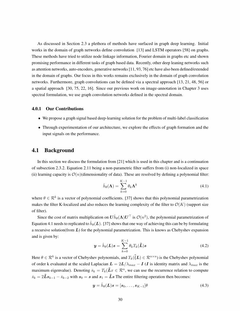
As discussed in Section 2.3 a plethora of methods have surfaced in graph deep learning. Initialworks in the domain of graph networks define convolution [13] and LSTM operators [58] on graphs.These methods have tried to utilize node linkage information, Fourier domain in graphs etc and shownpromising performance in different tasks of graph based data. Recently, other deep leaning networks suchas attention networks, auto-encoders, generative networks [11, 93, 76] etc have also been defined/extendedin the domain of graphs. Our focus in this works remains exclusively in the domain of graph convolutionnetworks. Furthermore, graph convolutions can be defined via a spectral approach [13, 21, 48, 56] ora spatial approach [30, 75, 22, 16]. Since our previous work on image-annotation in Chapter 3 usesspectral formulation, we use graph convolution networks defined in the spectral domain.

4.0.1 Our Contributions

• We propose a graph signal based deep-learning solution for the problem of multi-label classification

• Through experimentation of our architecture, we explore the effects of graph formation and theinput signals on the performance.

4.1 Background

In this section we discuss the formulation from [21] which is used in this chapter and is a continuationof subsection 2.3.2. Equation 2.11 being a non-parametric filter suffers from (i) non-localized in space(ii) learning capacity is O(n)(dimensionality of data). These are resolved by defining a polynomial filter:

hθ(Λ) =

K−1∑k=0

θkΛk (4.1)

where θ ∈ Rk is a vector of polynomial coefficients. [37] shows that this polynomial parametrizationmakes the filter K-localized and also reduces the learning complexity of the filter to O(K) (support sizeof filter).

Since the cost of matrix multiplication on U hθ(Λ)U> is O(n2), the polynomial parametrization ofEquation 4.1 needs to replicated to hθ(L). [37] shows that one way of achieving this can be by formulatinga recursive solution(from L) for the polynomial parametrization. This is knows as Chebyshev expansionand is given by:

y = hθ(L)s =

K−1∑k=0

θkTk(L)s (4.2)

Here θ ∈ Rk is a vector of Chebyshev polynomials, and Tk ((L) ∈ Rn×n) is the Chebyshev polynomialof order k evaluated at the scaled Laplacian L = 2L/λmax − I (I is identity matrix and λmax is themaximum eigenvalue). Denoting sk = Tk(Lx ∈ Rn, we can use the recurrence relation to computesk = 2Lsk−1 − sk−2 with s0 = s and s1 = Ls The entire filtering operation then becomes:

y = hθ(L)s = [s0, . . . , sK−1]θ (4.3)

30

The entire cost of operations for this parametrization then becomes O(K|E|).The final output feature map for a sample t is given by:

yt,j =

Fin∑i=1

hθi,j (L)st,i ∈ Rn (4.4)

where the st,iare the input feature maps, yt,j is the jth output feature map and the Fin × Fout vectors ofChebyshev coefficients θi,j ∈ Rk are the layers trainable parameter. We utilize Equation 4.4 to defineconvolution filter operation, henceforth in this chapter.

4.2 Proposed Approach

In this work, as mentioned before, we focus on finding an alternative approach to label modellingi.e. to model the label co-occurrence and dependency patterns. Recent works have approached this bymodelling labels as a sequence of words [98, 62] or by using graph based models [66] for propagatinglabels in a controlled way. Motivated by the recent developments in the graph deep learning, we focuson finding an alternative to [66]. Our proposed approach is depicted in Figure 4.1. Similar to the recentannotation models our models also utilizes the three modalities. Now, we describe them in detail:

4.2.1 Label Modelling

Our label model is graph based i.e. each node on the graph represents a label and the edges capture theinterrelations between them. Instead of explicitly expanding nodes as in [66], we focus on intrinsicallycapturing the flow of signals between different nodes of the graph by utilizing the spectral graphconvolution formulation of [21]. For our purposes, we require two inputs (i) a knowledge graph(fordefining L) which remains static for all the samples enabling a single eigen-decomposition of the laplacianmatrix and hence a constant graph Fourier basis. (ii) a graph signal which changes for each input signal.We now describe these inputs in detail:

4.2.1.1 Knowledge Graph

In most graph based applications, the knowledge graph (or adjacency matrix) is pre-defined, which,however, is not provided in any standard multi-label image recognition datasets. Capturing patterns oflabel dependence and co-occurrence in labels could be achieved by quantifying pairwise relation betweenthem. Since edges on the graph captures pairwise relationship, we use it to capture the label relations.

We use different sources of information to construct our knowledge graph. To define a graph weneed to define the nodes and edges(with weights). Our main idea to define edge weights is to countco-occurrence among labels. Using the train split of the dataset we count co-occurrences between each setof pairwise labels, and then discard all edges below a certain threshold. In particular we use 2 strategiesto weigh edges and define nodes in the knowledge graph:

31

• MSCOCO Graph: The node set in this graph consist of all the labels in the MSCOCO datasetie. 80 nodes. We use the trains set of MSCOCO dataset to define the edge weights. We set thepairwise occurrence threshold to 400, below which all edges are discarded.

• VGML enhanced graphs: We use Visual Genome[46] as an external source for our knowledgegraph. It consists of 100, 000 natural images which is annotated as objects, attributes and therelationships between them. We follow [66] to obtain 316 labels which forms the nodes of thegraph. These 316 labels consists of MSCOCO labels, 200 most frequently occurring objects 100

most frequently occurring attributes in Visual Genome (MSCOCO labels overlap with objects fromVisual Genome). We count the object-object and object-attribute pairwise occurrences and pruneedges having fewer than 200 instances. This knowledge graph is an external source of informationhence the model with this graph remains as a local approach in image annotations.

FRCNdetectionsPersonCowTable

KnowledgeGraph

Input Signals On Graph

Graph Convolution Layers

ConvolutionBlocks

PoolingBlocks

VGG16 (fc7 layer)

FullyConnected

Block

JointSpace Prediction

Image Representation

GraphSignals

Figure 4.1: Proposed approach: Given an input image, its representation is computed by passing itthrough VGG16(fc7 layer) network with pretrained weights. On other hand Faster-RCNN detectionsare passed as input signals to graph which undergoes through 2 stages of graph convolution and poolinglayers(as defined in [21]. Later both the above representations are concatenated and passed through afully connected neural net before final prediction. Note that colors denote activated(non-zero) signalsand the width of the edges denote different edge-weights. Notice that one of node is is inactive after 1st

convolution layer. This depicts that the diffusion of the signals is limited in the framework due to thechoice of the parameter K(=2 here) in Equation 4.3 (Best seen in color)

We ensure that our graph is connected, so that the signals may diffuse to all nodes/labels. This ensuresthat any two nodes which do not have an edge between them may still influence one-another by thevirtue of a path between them. In our initial experiments, we enhanced the edge weight by using cosinesimilarity between vector representations of labels, but the resulting performance was poorer.

32

4.2.1.2 Graph Signals

During training and testing, we need to provide a signal(x ∈ Rn) to each graph-node. We determinethe value on these signals based on likelihood of the concept being present in the image as determined byan object detector or a classifier. For our experiments, we use Faster R-CNN(FRCN) [77] for each of the80 MSCOCO categories. Instead of passing FRCN likelihood for all 80 categories, we binarize thesevalues above a certain threshold. Unless otherwise specified we set the this threshold at 0.5.

4.2.2 Image Representation

Following the trends of recent works of [62, 98] we use VGG(fc7 layer) to extract image representa-tion. This choice of network also help us in a direct comparisons of the models. We chose not to fine-tunethis part of the network as we focus on capturing the label dependencies for the graph convolutionnetworks.

4.2.3 Joint Space

Instead of learning a joint space to project the representations from the above stage, we chose to learna network to combine the signal representation and the image representation. Following the work of [66]we concatenate the representation of both the previous modalities and pass it through a fully-connectednetwork. Introducing a fully-connected block allows the whole model to be fully-differentiable. For theprediction we chose top-r labels with highest scores. The value of r is set as the mean labels per image inthe dataset(rounded off to the closest integer). In case of MSCOCO we set r as 3.

4.2.4 Network Architecture

Here, we provide detail about the Graph Convolutional Layers and Fully Connected Block as shownin Figure 4.1. We stack 2 layers of graph-convolution, each followed by a pooling layer (as defined in[21]) and an activation function (leaving the last layer). Similarly for Fully connected block we chose1 or 2 hidden-layers before the final prediction. Each such hidden layer in followed by an activationfunction.

4.2.5 Training and Network Parameters

Although our model is end-to-end trainable we train it in a greedy manner (fixing the weights for thedetector network- FRCN and for image representations-VGG). We set an initial learning rate of 1e− 4

while using an Adam optimizer, weight regularization of 5e− 4 for all parameters of graph convolutionlayers, batch-size of 16, and trained all our models till convergence (which turned out around 20 epochsfor most experiments). We set K=2 (Equation 4.4), number of filters( Equation 4.4) as 16, 32 respectivelyin graph convolution layers and the pooling scale 1 (i.e after each graph convolution block all the nodes

33

are retained). Relu was utilized as the activation function in Graph Convolution layers and in fullyconnected block. We use binary cross entropy loss to train our network.

4.3 Dataset

4.3.1 MSCOCO

2Microsoft COCO (MSCOCO) dataset [60] is an image-recognition, segmentation, and captioningdataset. It contains 123, 287 images pertaining to 11 super-categories which are further hierarchicallydivided into 80 objects categories. The images are predivided into two sets: training set and testingset. 82, 783 images are utilized as training set images while 40, 504 images are employed as testing setimages(Furthermore, 40, 775 images are hidden are used for the online leader-board for detection andcaptioning tasks. To obtain labels we utilize the object annotations. On average each image is labeledwith 2.9 tags and hence this forms a suitable dataset form multi-label image annotation.

The labelling of the MS-COCO dataset is done in three stages: (i) Super-Category labelling: In thisstage the annotators were asked to verify if a specific super-category was present in the image. (ii)Instance spotting: Here, annotators were asked to manually mark(a cross symbol) and annotate the objectcategory for each instance(found in the previous stage). (iii) Instance Segmentation: Here, annotatorswere asked to segment an object instance as detected in the previous stage. The labelling process wasalso supported by a verification stage where annotators discarded poorly segmented images and theannotation task was repeated for these images. This ensured good quality labelling i.e. the datasetwas void of incomplete labelling(un-labelled objects) and wrong labels. An interesting property ofthe MS-COCO dataset is that most images in this dataset contain multiple objects, and these objectsusually have strong co-occurrence dependencies. For example, baseball glove and sport ball have highco-occurrence probability, while zebra and cat never appear together.

The 11 super-categories are: Animal, vehicle, outdoor-objects, sports, kitchenware, food, furniture,appliances, electronics, indoor-objects and person & accessory. The 80 object categories are: person,chair, banana, handbag, skis, skateboard, bicycle. couch, microwave, umbrella, teddy-bear, hot-dog,snowboard, car, sink, toilet, apple, scissors, tie, potted-plant, motorcycle, tv, oven , book, keyboard, truck,fire-hydrant, stop-sign, sports-ball, bird, cow, toaster, boat, backpack, traffic-light, bowl, refrigerator,surfboard, broccoli, donuts, cat, airplane, bus, pizza, sandwich, suitcase, vase, dog, train, cellphone,wine glass, cup,tennis-racket, basket-ball, fork, carrot, cake, basketball-glove, kite, knife, mouse, horse,sheep, bed, dinning table, remote,zebra, hairdryer, spoon, Frisbee, orange, parking-meter, giraffe, bottle,elephant, laptop, clock, bear, toothbrush and bench.

34

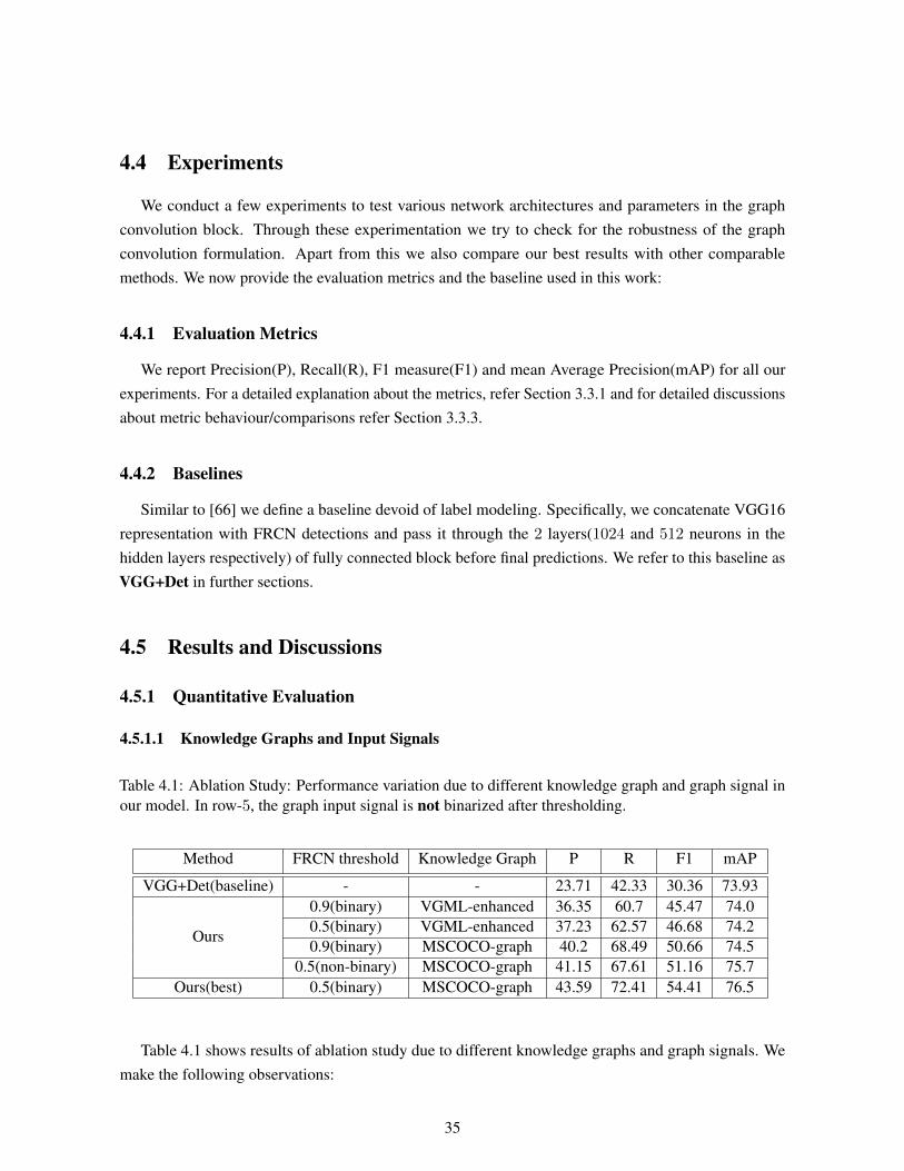
4.4 Experiments

We conduct a few experiments to test various network architectures and parameters in the graphconvolution block. Through these experimentation we try to check for the robustness of the graphconvolution formulation. Apart from this we also compare our best results with other comparablemethods. We now provide the evaluation metrics and the baseline used in this work:

4.4.1 Evaluation Metrics

We report Precision(P), Recall(R), F1 measure(F1) and mean Average Precision(mAP) for all ourexperiments. For a detailed explanation about the metrics, refer Section 3.3.1 and for detailed discussionsabout metric behaviour/comparisons refer Section 3.3.3.

4.4.2 Baselines

Similar to [66] we define a baseline devoid of label modeling. Specifically, we concatenate VGG16representation with FRCN detections and pass it through the 2 layers(1024 and 512 neurons in thehidden layers respectively) of fully connected block before final predictions. We refer to this baseline asVGG+Det in further sections.

4.5 Results and Discussions

4.5.1 Quantitative Evaluation

4.5.1.1 Knowledge Graphs and Input Signals

Table 4.1: Ablation Study: Performance variation due to different knowledge graph and graph signal inour model. In row-5, the graph input signal is not binarized after thresholding.

Method FRCN threshold Knowledge Graph P R F1 mAP

VGG+Det(baseline) - - 23.71 42.33 30.36 73.93

Ours

0.9(binary) VGML-enhanced 36.35 60.7 45.47 74.00.5(binary) VGML-enhanced 37.23 62.57 46.68 74.20.9(binary) MSCOCO-graph 40.2 68.49 50.66 74.5

0.5(non-binary) MSCOCO-graph 41.15 67.61 51.16 75.7Ours(best) 0.5(binary) MSCOCO-graph 43.59 72.41 54.41 76.5

Table 4.1 shows results of ablation study due to different knowledge graphs and graph signals. Wemake the following observations:

35

• We observe that MSCOCO graph works better than the VGML-enhanced graph consistently overall the metrics(Row-2 vs Row-4 and Row3 vs Row 6). This verifies our ideology that a combinationof global and local approaches is better than purely local or global approach. It may be possibleto design a generic-graph which is devoid of its dependency on the used data but doing so mayrequire manual enhancements.

• For graph input signals, higher threshold in FasterRCNN detections degrades the performance forboth VGML-enhanced and MSCOCO graphs(Row-2 vs Row-3 vs Row 4 vs Row-6). With higherthresholds fewer nodes have non-zero values(in graph signals) which may lead to incompletediffusion.

• We also observe that the performance from non-binarized input signals (for graphs) is poorer thenbinarized signal(Row-5 vs Row-6).

We hypothesize from the above observations that graph based deep learning approaches are susceptibleto underlying knowledge graphs (or adjacency matrices).

4.5.1.2 Comparison with other methods

Table 4.2: Comparison of popular methods on different evaluation metrics for MSCOCO dataset

Method P R F1 mAP

CNN-RNN [98] 69.2 66.4 67.8 61.2S-CNN-RNN [62] 77.41 73.05 75.16 -GSNN-VGG [66] - - - 77.57

VGG+Det(baseline) 23.71 42.33 30.36 73.93Ours 43.59 72.41 54.41 76.5

Table 4.2 provide a comparison of different popular label-modelling methods from the literature. Row1, 2 consists of methods that uses RNNs to model labels, whereas Row 3 uses graph LSTM networksto model labels. Our observation in Section 3.3.3 still remains valid: “the obvious understanding onecan make here is that there is non-agreement between F1 and mAP measures”. While comparing with[98, 62],we observe that our method is far behind in precision and F1 but is far better in mAP andperforms equivalent in recall. We also observe that the our method outperforms the baseline on all themetrics. While comparing with [66] we observed similar performance in the mAP scores1.

One of the potential reasons as to why our precision, recall and F1-scores are effected might be due toa fixed number of prediction per sample(3 in the case of MSCOCO) which increases the tags belongingfalse positives and false negatives. Models utilizing RNN and graph LSTMS can predict a variablenumber of samples and hence have fewer tags missing.

1At the time this work was done, authors of [66] did not release the code and were unresponsive on mail

36

4.5.2 Qualitative Results

Figure 4.2 shows the qualitative results on a 4 randomly selected samples from the MSCOCO dataset.The model misses on some of the obvious tags such as scissors and bottle in bottom-right and kite inbottom-left. This may also be possible as our model is fixed to predict 3 tags per sample. Detecting a fewtags might be tricky(as the tags are barely visible) as is the case with car in top-right.

Keyboard, Airplane, TV Bird, Person, Skateboard, Car

Umbrella, Boat, Surfboard, Kite Sheep, Person, Handbag, Suitcase, Bottle, Scissors

Figure 4.2: Qualitative results for label prediction on MSCOCO dataset. 4 randomly selected samplesand their predictions and ground truth labels(color coded). Green: Labels present in ground-truth andour model’s predictions (true positives), Blue: Incorrect predictions by the model (false positives). Red:Missed Predictions (false negatives) (Best seen in color)

37

Chapter 5

View Invariant Trajectory Mapping for Autonomous Driving

We take videos or image sequences as the input to perform the recognition task. The temporal infor-mation present inherently in such ordered image sequences leverages neighborhood information betweenframes, establishing relationships among objects in the scene. This also helps to mitigate the problem ofperceptual aliasing to some extent, a problem that often plagues image-based recognition/relocalizationapproaches.

We propose a novel stacked deep network ensemble architecture that combines state-of-the-artCNN, Bidirectional LSTM and Siamese style distance function learning for the task of view-invariantintersection recognition in videos. While the CNN component of the ensemble primarily deals withimage-level feature representation, the bidirectional LSTM is the key recurrent network component thatenables learning of temporal evolution of visual features in videos followed by the Siamese network-baseddistance metric learning for comparing two input video streams. Our proposed network is conceptualizedin Figure 5.1.

5.0.1 Contributions

In this published paper we contributed in the following ways:

1. Firstly, we propose a novel and pertinent problem of recognizing intersections when approachedfrom highly disparate viewpoints

2. We propose an original deep network ensemble. The proposed architecture can handle videos ofvarying length and compare videos capturing reverse trajectories. This kind of Siamese networkwith recurrent LSTM component has been largely unexplored in the video domain. Furthermore,we use the hidden state of LSTM cells, instead of the traditionally used output state, for videorepresentation, which has largely been unexplored too.

3. We showcase the efficacy of the proposed architecture through competitive results on challengingsequences while showing decent improvements from the image based baselines. We collect andannotate synthetic yet highly realistic data from the GTA [2] gaming platform and actual real worlddata of Mapillary [4] for this purpose.

38

To the best of our knowledge, this is the first attempt in this direction using the ensemble of state-of-the-artCNN, bidirectional LSTM and Siamese network architecture for recognizing intersection in input videopairs.

Distance function

Same Intersection? Yes/No

Shared

Weights

… …

……

……

InputPair

CNN

Bidirectional-LSTM Bidirectional-LSTM

Figure 5.1: Proposed model is shown with video pairs as input and binary-classification as the output.Features from pretrained CNN network are fed into bidirectional LSTM with shared-weights as shownwith hidden units in green (unfolded in time).

5.1 Proposed Approach

In order to achieve view-invariant intersection recognition from video sequences, our overall approachfollows the recent successes of deep network models in learning useful representations of visual data[9]. Our overall strategy comprises of three specific sub-objectives: (i) capture representations ofindividual video frames that can help identify the intersection in a view-invariant manner; (ii) leverage thetemporal correlations between video frames to better capture the unique identity of an intersection acrossdifferent views; and (iii) use an appropriate distance metric to compare the thus learned spatiotemporalrepresentations of intersection video sequences. We use a stacked deep network ensemble architecture torealize the above strategy.

Our stacked ensemble consists of a state-of-the-art Convolutional Neural Network (CNN) to learnvideo frame representations, a Bidirectional Long Short-Term Memory (LSTM) Network (a variantof Recurrent Neural Networks, that addresses the vanishing gradient problem) that captures temporalcorrelations across video frames, and a Siamese Network that learns a suitable distance metric that canuniquely identify an intersection from these video sequences across views. Figure 5.1 summarizes theproposed ensemble strategy.

39

5.1.1 Convolutional Neural Networks (CNNs)

CNN based models have shown tremendous success in a variety of tasks like [50], [7], etc. and ithas been shown that representations learned by the CNN can be used as off-the-shelf features for othertasks [83], [89].

From a plethora of CNN pretrained models, we choose the model most relevant to our tasks whichprovide invariance in lighting and pose. In particular, we employ AmosNet [17] as our CNN architecture.AmosNet is a variation of CaffeNet [50] trained for Visual Places Recognition under varying weatherconditions. We use pooled outputs from last convolution layer of AmosNet as the CNN features.

5.1.2 Bidirectional LSTM

Long Short-Term Memory Network (LSTM) [39], is a variant of Recurrent Neural Network (RNN)with the ability to capture long-term dependencies [47]. It has a hidden representation which is updatedat each time step, and also consists of a memory state which holds the relevant information at each timestep. The information entering and exiting out of cell states is controlled by gating mechanisms (sigmoid,and tanh functions).

Bidirectional LSTMs [82] incorporate future and past context by running the inverse of the inputthrough a separate LSTM. The proposed model employed Bidirectional LSTMs capture the temporalcorrelations between video frames. This enables our model to identify the intersection uniquely whethera vehicle approaches it in the forward or opposite direction. Instead of using averaged/fused output ofunfolded LSTM units or output from last unit we use the hidden-representation from the last unfoldedtime step as a feature vector for the videos as shown in Figure 5.1.

5.1.3 Siamese Network

The third component of our deep network ensemble is a Siamese network, which is used to learndata-driven distance metrics. A Siamese Network [103] consists of two independent networks with samearchitecture and shared weights. Both these networks are merged to learn a distance metric, d, betweenthe two inputs provided to the respective networks.

During training, Siamese networks work on triplets (x1, x2, y) where y is the ground truth similaritybetween x1 and x2, i.e., y = 1 if the videos denote the same intersection, else y = 0. The networks’weights are then updated by minimizing the loss function described below.

Contrastive Loss: The total loss function over a dataset X = {(xi1,xi2, yi),∀i = 1, · · · , n} is givenby:

LW (X) =

n∑i=1

LiW ((φ(xi1), φ(xi2)), yi) (5.1)

40

where W are the weights/parameters of the network, φ(x) denotes the output of the last layer of theshared network architecture for each individual input x, and LiW is

LiW = yiLpos(φ(xi1), φ(xi2)) + (1− yi)Lneg(φ(xi1), φ(xi2)) (5.2)

where

Lpos(φ(xi1), φ(xi2)) = d(φ(x1), φ(x2))2 (5.3)

Lneg(φ(xi1), φ(xi2)) = max (1− d(φ(x1), φ(x2)), 0)2 (5.4)

At test time, the learned distance function is used to predict the similarity in the videos using theexpression in Eq. 5.5.

y =

{0 : d(φ(x1), φ(x2)) > θ

1 : d(φ(x1), φ(x2)) ≤ θ(5.5)

We set the value of θ to be 0.5 in our experiments. Since the number of possible negative pairs can bevery high as compared to positive pairs, we scale the loss function for each positive by a constant factor(> 1), given by the ratio of negative pairs to positive pairs in the dataset.

5.1.4 Training and Network Parameters

Although our model can be trained in an end to end manner we train it in a greedy way due tonegligible effect on performance as compared to end-to-end training. We use pretrained weights fromprevious state-of-the-art CNN models which provide a meaningful weight-initialization to our model andreduces training time. We use the contrastive loss described in Eq. 5.1 to train the Bidirectional LSTM,as shown in Figure 5.1. The proposed model is trained using the ADAM optimizer which is a variant ofStochastic Gradient Descent (SGD).

In our initial experiments, we varied the number of Bidirectional LSTM-layers (upto 3), but theperformance gain was negligible. Similarly, we experimented with different values for hidden-unitdimensions in the LSTM cell. Empirical results found 250 to be the best performing after which theperformance saturates. Thus, we fix the number of Bidirectional layer to one and hidden layer dimensionto be 250 in all further experiments.

5.2 Experiments & Results

In this section, we first define the baselines used for comparison with our proposed method. Next, weproceed to provide description about synthetically generated and real datasets for various experiments.Subsequently we describe the various experimental scenarios which is followed by the explanation of thequantitative and qualitative results.

41

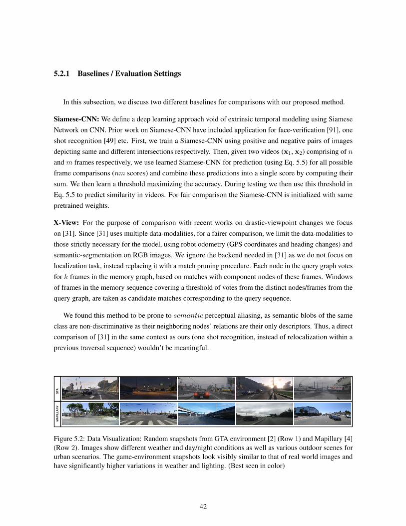
5.2.1 Baselines / Evaluation Settings

In this subsection, we discuss two different baselines for comparisons with our proposed method.

Siamese-CNN: We define a deep learning approach void of extrinsic temporal modeling using SiameseNetwork on CNN. Prior work on Siamese-CNN have included application for face-verification [91], oneshot recognition [49] etc. First, we train a Siamese-CNN using positive and negative pairs of imagesdepicting same and different intersections respectively. Then, given two videos (x1, x2) comprising of nand m frames respectively, we use learned Siamese-CNN for prediction (using Eq. 5.5) for all possibleframe comparisons (nm scores) and combine these predictions into a single score by computing theirsum. We then learn a threshold maximizing the accuracy. During testing we then use this threshold inEq. 5.5 to predict similarity in videos. For fair comparison the Siamese-CNN is initialized with samepretrained weights.

X-View: For the purpose of comparison with recent works on drastic-viewpoint changes we focuson [31]. Since [31] uses multiple data-modalities, for a fairer comparison, we limit the data-modalities tothose strictly necessary for the model, using robot odometry (GPS coordinates and heading changes) andsemantic-segmentation on RGB images. We ignore the backend needed in [31] as we do not focus onlocalization task, instead replacing it with a match pruning procedure. Each node in the query graph votesfor k frames in the memory graph, based on matches with component nodes of these frames. Windowsof frames in the memory sequence covering a threshold of votes from the distinct nodes/frames from thequery graph, are taken as candidate matches corresponding to the query sequence.

We found this method to be prone to semantic perceptual aliasing, as semantic blobs of the sameclass are non-discriminative as their neighboring nodes’ relations are their only descriptors. Thus, a directcomparison of [31] in the same context as ours (one shot recognition, instead of relocalization within aprevious traversal sequence) wouldn’t be meaningful.

Figure 5.2: Data Visualization: Random snapshots from GTA environment [2] (Row 1) and Mapillary [4](Row 2). Images show different weather and day/night conditions as well as various outdoor scenes forurban scenarios. The game-environment snapshots look visibly similar to that of real world images andhave significantly higher variations in weather and lighting. (Best seen in color)

42

Table 5.1: Number of video pairs in training, testing and the validation set for the different experimentalscenarios

Dataset→ GTALighting Setting→ day and night day

Trajectory Relations→ All combinations Overlap in view and trajectory All combinations

Train1509 640 8641440 1440 1166

Val459 168 300612 212 653

Test106 62 72104 104 82

Dataset→ MapillaryLighting Setting→ day

Trajectory Relations→ All combinations Overlap in view and trajectory

Train3080 64093328 6976

Val421 350428 318

Test400 425400 420

5.2.2 Dataset Description

Dataset Collection: Each video/sequence consist of a series of frames collected around junction points.Each junction can be traversed in multiple pathways. We refer to the set of all such possible traversals astrajectories.

5.2.2.1 GTA

Here, we collected videos in two different scenarios. Firstly, we choose a set of intersections in thegame-environment and then sample them in a dense manner, i.e., each possible trajectory in the junctionis traversed. Secondly, we traversed a car from one point to another via means of an AI-car drivingmod [3]. From such traversals, we break the captured video into small chunks involving intersectionsand non-intersections. We discard video chunks without intersections.

In the first scenario, we selected 27 unique junctions where 9 of them had arbitrary lighting conditionsand the rest were in normal daylight condition. In the second scenario, we captured 12 traversals in twoarbitrary different lighting variations.

43

5.2.2.2 Mapillary

We download images from [4], which is a community-led service with more than 200 million street-level images. These images are captured in various modes including walking, riding (either a bike or car),panorama and photo-spheres. We use mapillary’s API to download images and construct trajectories. Wefirst query for all the images in a bounding box defined by the longitudes and latitudes. For every imagein the bounding box, the API provides a tuple consisting of image-key, latitude, longitude, orientationand the (video-)sequence it belongs to along with other metadata information. These images can be thendownloaded using the image-key. Using two orthogonally overlapping sequences we get a location in themap which is used to identify the intersection. Subsequently, this is used to download all sequences ( aset of continuous images) passing through that intersection. We mined around 300, 000 images whichconsisted of around 1700 usable sequences from around 500 junctions.

Figure 5.2 shows random snapshots captured from GTA environment (Row 1) and Mapillary (Row2). One can infer from the figure that the snapshots from GTA environment are visually realistic aswell as similar to real-world data from Mapillary and contain the key challenges associated with realenvironments (as listed in Section 1.3). However, the GTA environment offers more complexity in termsof weather and lighting variations as compared to Mapillary.Dataset Annotation: From the extracted dataset, we first annotate positive and negative video pairs.Positive (videos involving the same intersection) pairs are mined from the above datasets exhaustively,i.e., we select all possible positive pairs. Negative pairs generated from the datasets can be very high asany two trajectories from different junction are treated as a negative pair. Hence we limit the number ofnegative pairs by randomly fixing a subset. We keep the test, train and validation sets mutually exclusiveby sampling them from different junction and/or non-overlapping traversals.

Table 5.2: Accuracy, Precision, Recall and F1 of our method on different datasets for the differentexperimental scenarios

MetricsDataset→ Mapillary

Lighting Setting→ day↓ Trajectory Relations→ All combinations Overlap in view and trajectory

AccuracyOur Method 72.1 81.0

Siamese CNN 63.0 71.6

F1 ScoreOur Method 61.9 82.4

Siamese CNN 428 318

MetricsDataset→ GTA

Lighting Setting→ day and night day↓ Trajectory Relations→ All combinations Overlap in view and trajectory All combinations

AccuracyOur Method 70.95 78.2 76.72

Siamese CNN 65.3 65.3 68.0

F1 ScoreOur Method 62.3 60.0 72.7

Siamese CNN 47.9 52.8 51.1

44

5.2.3 Experimental Setup

For a pair of videos involving the same junction there exists a trajectory-relation between them, whichcan be categorized in terms of overlap in view and/or trajectory. Overlap in trajectory refers to theproximal relation in the two trajectories while overlap in view refers to trajectories, viewing the largerpart of the same area. For example trajectories moving in opposite direction can be proximal in distancebut can have minimal view overlap.

For the purpose of our experiments we categorize the trajectory-relations into two primary setups:Overlap in view and trajectory and All combinations. The former refers to parallel and overlappingtrajectory-relations while the latter refers to all the possible trajectory-relations. Similarly, we categorizethe lighting setting into two categories: day vs day and night. The names are self-explanatory.

We test the robustness and generalizing capability of our model under various trajectory-relation andlighting (day/night) settings. The details of the experiment-wise distribution of samples can be found inTable 5.1.

Evaluation Metric: We report percentage accuracy and F1 as the metric in our experiments. Accuracyis defined as the ratio of the number of correctly classified samples (both positive and negative pairscombined) to the total predictions made. F1 is defined as the harmonic mean of precision and recall. Wenote that while accuracy focuses on both positive and negative predictions, F1 is focused toward positivepredictions (as precision and recall focuses on true-positives).

5.2.4 Quantitative Results

Table 5.2 shows performance on various metrics on GTA and Mapillary dataset under varyingscenarios using our proposed model and baseline Siamese-CNN. We show different comparisons basedon lighting setting, trajectory relation and baseline approach.

GTA: We observe that our proposed method performs better than the Siamese-CNN baseline on bothAccuracy and F1. Additionally, among different models in the proposed approach (for different lightingconditions) we observe that the model improves on accuracy (by 5.76%) and F1 (by 10.4%) in dayscenario as compared to day and night scenario. Similar trend of values is also observed in the Siamese-CNN baseline. This trend of results can be attributed to the reduced complexity in lighting variations.

Interestingly, under the day and night condition, the model performs better at accuracy (7.25%

increase) when video-pairs have an Overlap in view and trajectory as compared to All combinations.However we observed an inverse trend for F1 measure. This anomalous behavior can be explained basedon the performance on negative samples in this scenario. In this case we found that the true negative ratesperformance for Overlap in view and trajectory is 83.0% as compared to All combinations at 52.8% (30%

increase). Nevertheless, the performance of proposed model is still significantly higher than baselinemethod.

Mapillary: Similar to GTA, we observe that our proposed method performs better than the Siamese-CNNbaseline on both accuracy and F1. Among models in our proposed method, the performance is better

45

Table 5.3: X-View results on Mapillary: F1-scores at different experimental threshold (query sequencelength: 15)

Localization Threshold Inlier Frames % F120m 70 51.540m 70 50.940m 80 47.760m 70 43.760m 80 46.7

on all metrics (accuracy: 8.9%increase, F1:20.5%increase) when the trajectory-relations are limitedto Overlap in view and trajectory as compared to All combinations. Similar change in values can beobserved in the Siamese-CNN baseline.

GTA vs Mapillary (for proposed method): In the common scenario of day and All combinations, wenotice that the performance on GTA is better than Mapillary for accuracy (4.62% increase) and F1 (10.8%

increase). This can be explained due to complexity of data annotation in real-world where visuallydis-similar videos can be annotated as same based on their GPS coordinates.

Table 5.3 shows experimental results of X-view on Mapillary in relocalisation scenarios. We used 12

relevant and reliably segmented semantic categories. Localisation Threshold(maximum distance fromGround Truth for a match) and Inlier Frames%(% of dictinct valid frames voting for a window of framesin the memory sequence) were varied to obtain the best F1 scores. We observe that F1 scores obtainedare always lower than F1 scores for Mapillary data in Table 5.2. The method had high recall but lowprecision across multiple thresholds. This can partly be attributed to the fact that [31] requires 15 or moreoverlapping frames for reliable localization whereas in case of orthogonal trajectories in Mapillary only5-7 frames have overlapping structures.

5.2.5 Qualitative Results

Figure 5.3 shows 3 positive samples from Mapillary that are successfully predicted by the network.Each sample depict a unique trajectory-relation and view-overlap as shown by the intersection-map(bottom-most row). We color encode (green, cyan, red, brown) the visually perceptible common structures(using ellipses) in the trajectories. We follow the same encoding while plotting the respective intersection-map in the last row. In video pair 1 and video pair 3, we observe that the overlapping part of trajectoriesare in the opposite direction but our network managed to exploit the common structures seen fromdifferent views. In video pair 2, though the partially overlapping trajectories are in the same direction,we can observe that shadows pose a challenge that is successfully handled by the network. This indicatethe ability of proposed network to generalize on varying lighting conditions. Moreover, we also observeocclusion in a few trajectories (video pair 3 trajectory 2) due to vehicles.

46

Traj

. 1Tr

aj. 2 Vid

eo P

air 1

Traj

. 1Tr

aj. 2

Vid

eo P

air 2

Vid

eo P

air 2

Vid

eo P

air 1

Vid

eo P

air 3

Traj

. 1Tr

aj. 2

Vid

eo P

air 3

Figure 5.3: Three correctly classified samples from Mapillary. Each sample depicts unique trajectory-relation and view-overlap between trajectories as shown in the intersection-map (bottom-most row)which represents the top-view of the intersection. We color encode the visually perceptible commonstructures (cyan, green, red, brown) in the Video pairs. Video pair 2 and Video pair 3 show exampleswhere trajectory direction and view overlap. Video pair 1 depict cases when the overlap in trajectoriesand/or the view is minimal. (Best seen in color)

Figure 5.4 depicts 2 positive samples from GTA that are successfully predicted by the network. Forexample: video-pair 1, capture the different view of the same structure in rainy weather. Similarly, invideo-pair 2 the model is able to predict similar videos in presence of view and lighting variations. Dueto space constraints we only show 6 aligned contiguous frames in these video-pairs, where we manuallycrop the relevant contiguous frames for illustration purpose.

Figure 5.5 shows some incorrect predictions made by the network. Video pair 1 consist of trajectoriesfrom different intersections (negative sample) but is predicted as the same intersection. We believe thismay be due to lack of unique structures in the scene as most of it has trees. Additionally, the variance inlighting conditions (as the network was trained on day conditions in Mapillary) can also pose a challengeif not trained on other conditions. In contrast, video pair 2 are trajectories from the same-intersection butare predicted as different intersection. In this video pair, we observe a complete lack of visual features in

47

Traj

. 1Tr

aj. 2

Vid

eo P

air 1 Tr

aj. 1

Traj

. 2 V

ideo

Pai

r 2

Figure 5.4: Two correctly classified samples from GTA. Video pair 2 show examples where trajectorydirection and view overlap. Video pair 1 depict case when the overlap in trajectories and/or the view isminimal. (Best seen in color)

Traj

. 1Tr

aj. 2 Vid

eo P

air 1

Traj

. 1Tr

aj. 2 Vid

eo P

air 2

Traj

. 1Tr

aj. 2 V

ideo

Pai

r 3

Figure 5.5: Failure Cases: Three wrong predictions by the network. Video pair 1 consist of trajectoriesfrom different intersections but is predicted as the same intersection. In contrast, video pair 2, 3 consistof trajectories from the same-intersection but are predicted as different intersection

48

the overlapping part of trajectories. Overlapping structures are completely occluded in the first trajectorydue to the presence of truck. Using purely visual content for all these failure cases, even humans mighteasily fail without extra context (ground truth labels were generated using GPS coordinates). Similarto video pair 2, video pair 3 trajectories belong to the same intersection but are predicted as different.Biased on the grounds of pure visual content, the video-pair does not contain a common region of interestand hence can be argued that the prediction from the network is correct.

To further showcase some negative results of our model we present some more qualitative results inFigures 5.6, 5.7. Each of the video depicted here consists of 14 frames which is in contrast to Figures 5.3,5.5 which consisted of 10-11 frames. We show more frames in these figures to reinforce the complexdata, temporal and visual complexity of the problem at hand.

Figure 5.6 shows examples of false positives, that is, each video pair consist of video from differentintersections but is predicted as to be same. We observe that the visual similarity makes it harder forthe network to classify the trajectories as different samples. Since our method is based just on a visualmethod, we believe that such errors are justified/acceptable.

Vid

. 2V

id. 1

V

ideo

Pai

r 2V

id. 2

Vid

. 1

Vid

eo P

air 1

Figure 5.6: Failure Cases(False Positives): Two wrong predictions by the network. Video pair 1 and2 consists of trajectories from different intersections but is predicted as the same intersection. Boththe trajectories in Video-Pair 1 capture the side-view of the road traversal which adds to complexity ofintersection recognition. Video-Pair 2 is in fact a true failure case and we believe sch errors are acceptabledue to the sufficient visual similarity in the videos.

We further showcase 2 false negatives that is the network predicted the pair of trajectories as differentwhile they belonged to the same intersection as shown in Figure 5.7. We hypothesize that the networkfailed to find the static parts (such as common buildings view points) in these trajectories and hence failedto identify them belonging to the same intersection.

49

Vid

. 2V

id. 1

V

ideo

Pai

r 2V

id. 2

Vid

. 1

Vid

eo P

air 1

Figure 5.7: Failure Cases(False Negatives): Two wrong predictions by the network. These Video pairsbelonged to the same intersection but were predicted as different by the network.

50

Chapter 6

Conclusion

Scene understanding entails enabling machines to understand scenes, similar to humans’ understandingof it. Thus, scene understanding engulfs a wide array of problems involving visual data. Recent outburstof visual data has facilitated fast paced development of this field. In this thesis we restrict ourselves toa couple of problems namely image annotation and intersection recognition from the domain of sceneunderstanding.

In Chapter 3, we presented a solution for automatic multi-label image annotation. Our methodexploits the empirical observation that similar images have similar neighborhood-types in terms of theirlabel distribution. We have introduced the notion of neighborhood-type and proposed to learn localMKL models per cluster/neighborhood-type with closed form learning solution. The MKL formulationexploits the multi-scale diffusion where we also proposed a novel diffusion scale normalization to beable to combine diffusion at different local graphs. Finally, we have shown promising results on publiclyavailable dataset. Capturing higher order relations with the help of hyper-graphs and development ofdeep hyper-graph networks is one of the potential directions for future work.

In Chapter 4, we presented an alternate approach for label modelling using the newly rising field ofgraph deep networks. Our model utilizes the graph convolution formulation by Defferrard et. al.[21]. Weexplore weather label modelling from such graph networks formulations are comparable with traditionaldeep learning approaches. Further, we focused on testing the robustness of the model to different(graph)input signals and different knowledge graph formulations. Although our work here is on imageannotation involving two modalities of data: images and labels, we believe that hybrid- deep learningmodels(i.e. models with graph networks and regular grid networks) can be used to model multiplemodalities of data and combine them efficiently.

In Chapter 5, we proposed a stacked deep network ensemble architecture that combines state-of-the-artCNN, bidirectional LSTM and Siamese style distance function learning for the task of view-invariantintersection recognition in videos. The proposed architecture enables recognizing the same intersectionacross two videos of variable length having large view variations, inverted trajectory, lightning andweather variations. We have collected annotated data (more than 2000 videos) from GTA [2] andMapillary [4] and have computed results on this data with varying parameter choices and have reportedcompetitive results.

51

Related Publications

1. MKL based Local Label Diffusion for Automatic Image Annotation [51]National Conference on Computer Vision, Pattern Recognition, Image Processing and Graphics(NCVPRIPG), 2017 [Oral Presentation]Abhijeet Kumar, Anjali Anil Shenoy and Avinash Shrama.CVIT, KCIS, International Institute of Information Technology, Hyderabad

2. Towards View-Invariant Intersection Recognition from Videos using Deep NetworkEnsembles [Short Oral Presentation] [52]International Conference on Intelligent Robots and Systems (IROS), 2018Abhijeet Kumar†, Gunshi Gupta†, Avinash Sharma and K. Madhav KrishnaCVIT, RRC, KCIS, International Institute of Information Technology, Hyderabad

† Authors contributed Equally

52

Bibliography

[1] Gardens Point Dataset. https://wiki.qut.edu.au/display/cyphy/Day+and+Night+

with+Lateral+Pose+Change+Datasets.

[2] Grand Theft Auto V. https://en.wikipedia.org/wiki/Development_of_Grand_

Theft_Auto_V.

[3] Grand Theft Auto V Auto-drive Mod. https://www.gta5-mods.com/scripts/vautodrive.

[4] Mapillary. https://www.mapillary.com/app.

[5] S. Achar, C. V. Jawahar, and K. M. Krishna. Large scale visual localization in urban environments. In

ICRA, 2011.

[6] A. Angeli, D. Filliat, S. Doncieux, and J. Meyer. Fast and incremental method for loop-closure detection

using bags of visual words. TRO, 2008.

[7] V. Badrinarayanan, A. Kendall, and R. Cipolla. SegNet: A deep convolutional encoder-decoder architecture

for image segmentation. arXiv preprint arXiv:1511.00561, 2015.

[8] K. Barnard, P. Duygulu, D. Forsyth, N. d. Freitas, D. M. Blei, and M. I. Jordan. Matching words and

pictures. Journal of machine learning research, 3(Feb):1107–1135, 2003.

[9] Y. Bengio, A. Courville, and P. Vincent. Representation learning: A review and new perspectives. TPAMI,

2013.

[10] D. Bhatt, D. Sodhi, A. Pal, V. Balasubramanian, and K. M. Krishna. Have I reached the intersection: A

deep learning-based approach for intersection detection from monocular cameras. In IROS, 2017.

[11] A. Bojchevski, O. Shchur, D. Zugner, and S. Gunnemann. Netgan: Generating graphs via random walks.

arXiv preprint arXiv:1803.00816, 2018.

[12] M. M. Bronstein, J. Bruna, Y. LeCun, A. Szlam, and P. Vandergheynst. Geometric deep learning: going

beyond euclidean data. CoRR, abs/1611.08097, 2016.

[13] J. Bruna, W. Zaremba, A. Szlam, and Y. LeCun. Spectral networks and locally connected networks on

graphs. arXiv preprint arXiv:1312.6203, 2013.

[14] G. Carneiro, A. B. Chan, P. J. Moreno, and N. Vasconcelos. Supervised learning of semantic classes

for image annotation and retrieval. IEEE transactions on pattern analysis and machine intelligence,

29(3):394–410, 2007.

53

[15] H. Cevikalp, B. Benligiray, O. N. Gerek, and H. Saribas. Semi-supervised robust deep neural networks

for multi-label classification. In Proceedings of the IEEE Conference on Computer Vision and Pattern

Recognition Workshops, pages 9–17, 2019.

[16] J. Chen, T. Ma, and C. Xiao. Fastgcn: fast learning with graph convolutional networks via importance

sampling. arXiv preprint arXiv:1801.10247, 2018.

[17] Z. Chen, A. Jacobson, N. Sunderhauf, B. Upcroft, L. Liu, C. Shen, I. Reid, and M. Milford. Deep learning

features at scale for visual place recognition. arXiv preprint arXiv:1701.05105, 2017.

[18] Z.-M. Chen, X.-S. Wei, P. Wang, and Y. Guo. Multi-label image recognition with graph convolutional

networks. In Proceedings of the IEEE Conference on Computer Vision and Pattern Recognition, pages

5177–5186, 2019.

[19] F. Chung. Spectral Graph Theory. Number no. 92 in CBMS Regional Conference Series. Conference

Board of the Mathematical Sciences.

[20] S. Datta, S. Tourani, A. Sharma, and K. M. Krishna. Slam pose-graph robustification via multi-scale

heat-kernel analysis. In Decision and Control (CDC), 2016 IEEE 55th Conference on, pages 2912–2919.

IEEE, 2016.

[21] M. Defferrard, X. Bresson, and P. Vandergheynst. Convolutional neural networks on graphs with fast

localized spectral filtering. In Advances in neural information processing systems, pages 3844–3852, 2016.

[22] T. Derr, Y. Ma, and J. Tang. Signed graph convolutional networks. In 2018 IEEE International Conference

on Data Mining (ICDM), pages 929–934. IEEE, 2018.

[23] A. Dosovitskiy, G. Ros, F. Codevilla, A. Lopez, and V. Koltun. CARLA: An open urban driving simulator.

In CoRL, 2017.

[24] D. K. Duvenaud, D. Maclaurin, J. Iparraguirre, R. Bombarell, T. Hirzel, A. Aspuru-Guzik, and R. P. Adams.

Convolutional networks on graphs for learning molecular fingerprints. In Advances in neural information

processing systems, pages 2224–2232, 2015.

[25] P. Duygulu, K. Barnard, J. F. de Freitas, and D. A. Forsyth. Object recognition as machine translation:

Learning a lexicon for a fixed image vocabulary. In European conference on computer vision, pages 97–112.

Springer, 2002.

[26] M. Everingham, L. Van Gool, C. K. Williams, J. Winn, and A. Zisserman. The pascal visual object classes

(voc) challenge. International journal of computer vision, 88(2):303–338, 2010.

[27] S. Feng, R. Manmatha, and V. Lavrenko. Multiple bernoulli relevance models for image and video

annotation. In null, pages 1002–1009. IEEE, 2004.

[28] H. Fu, Q. Zhang, and G. Qiu. Random forest for image annotation. In European Conference on Computer

Vision, pages 86–99. Springer, 2012.

[29] D. Galvez-Lopez and J. D. Tardos. Bags of binary words for fast place recognition in image sequences.

TRO, 2012.

54

[30] H. Gao, Z. Wang, and S. Ji. Large-scale learnable graph convolutional networks. In Proceedings of the

24th ACM SIGKDD International Conference on Knowledge Discovery & Data Mining, pages 1416–1424.

ACM, 2018.

[31] A. Gawel, C. Del Don, R. Siegwart, J. Nieto, and C. Cadena. X-view: Graph-based semantic multi-view

localization. arXiv preprint arXiv:1709.09905, 2017.

[32] A. Glover, W. Maddern, M. Warren, S. Reid, M. Milford, and G. Wyeth. OpenFABMAP: An open source

toolbox for appearance-based loop closure detection. In ICRA, 2012.

[33] D. Grangier and S. Bengio. A discriminative kernel-based model to rank images from text queries. IEEE

Transactions on Pattern Analysis and Machine Intelligence (TPAMI), 10(LIDIAP-ARTICLE-2008-010),

2008.

[34] M. Guillaumin, T. Mensink, J. Verbeek, and C. Schmid. Tagprop: Discriminative metric learning in nearest

neighbor models for image auto-annotation. In Computer Vision, 2009 IEEE 12th International Conference

on, pages 309–316. IEEE, 2009.

[35] H. Guo, K. Zheng, X. Fan, H. Yu, and S. Wang. Visual attention consistency under image transforms for

multi-label image classification. In The IEEE Conference on Computer Vision and Pattern Recognition

(CVPR), June 2019.

[36] A. A. Hafez, M. Singh, K. M. Krishna, and C. V. Jawahar. Visual localization in highly crowded urban

environments. In IROS, 2013.

[37] D. K. Hammond, P. Vandergheynst, and R. Gribonval. Wavelets on graphs via spectral graph theory. Applied

and Computational Harmonic Analysis, 30(2):129–150, 2011.

[38] M. Henaff, J. Bruna, and Y. LeCun. Deep convolutional networks on graph-structured data. arXiv preprint

arXiv:1506.05163, 2015.

[39] S. Hochreiter and J. Schmidhuber. Long short-term memory. Neural computation, 1997.

[40] H. Hu, G.-T. Zhou, Z. Deng, Z. Liao, and G. Mori. Learning structured inference neural networks with

label relations. In Proceedings of the IEEE Conference on Computer Vision and Pattern Recognition, pages

2960–2968, 2016.

[41] M. J. Huiskes and M. S. Lew. The mir flickr retrieval evaluation. In Proceedings of the 1st ACM international

conference on Multimedia information retrieval, pages 39–43. ACM, 2008.

[42] J. Jeon, V. Lavrenko, and R. Manmatha. Automatic image annotation and retrieval using cross-media

relevance models. In Proceedings of the 26th annual international ACM SIGIR conference on Research and

development in informaion retrieval, pages 119–126. ACM, 2003.

[43] J. Jin and H. Nakayama. Annotation order matters: Recurrent image annotator for arbitrary length image

tagging. In 2016 23rd International Conference on Pattern Recognition (ICPR), pages 2452–2457. IEEE,

2016.

[44] J. Johnson, L. Ballan, and L. Fei-Fei. Love thy neighbors: Image annotation by exploiting image metadata.

In Proceedings of the IEEE international conference on computer vision, pages 4624–4632, 2015.

55

[45] M. M. Kalayeh, H. Idrees, and M. Shah. Nmf-knn: Image annotation using weighted multi-view non-

negative matrix factorization. In Proceedings of the IEEE conference on computer vision and pattern

recognition, pages 184–191, 2014.

[46] A. Karpathy and L. Fei-Fei. Deep visual-semantic alignments for generating image descriptions. In

Proceedings of the IEEE conference on computer vision and pattern recognition, pages 3128–3137, 2015.

[47] A. Karpathy, J. Johnson, and L. Fei-Fei. Visualizing and understanding recurrent networks. arXiv preprint

arXiv:1506.02078, 2015.

[48] T. N. Kipf and M. Welling. Semi-supervised classification with graph convolutional networks. arXiv

preprint arXiv:1609.02907, 2016.

[49] G. Koch, R. Zemel, and R. Salakhutdinov. Siamese neural networks for one-shot image recognition. In

ICML-W, 2015.

[50] A. Krizhevsky, I. Sutskever, and G. E. Hinton. Imagenet classification with deep convolutional neural

networks. In NIPS, 2012.

[51] A. Kumar, A. A. Shenoy, and A. Sharma. Mkl based local label diffusion for automatic image annotation.

Sixth National Conference on Computer Vision, Pattern Recognition, Image Processing, and Graphics.

NCVPRIPG 2017, 841:385–399, 2017.

[52] A. Kumar, A. A. Shenoy, and A. Sharma. Towards view-invariant intersection recognition from videos

using deep network ensembles. IEEE/RSJ International Conference on Intelligent Robots and Systems.

IROS 2018, 2018.

[53] V. Lavrenko, R. Manmatha, and J. Jeon. A model for learning the semantics of pictures. In Advances in

neural information processing systems, pages 553–560, 2004.

[54] D. D. Lee and H. S. Seung. Algorithms for non-negative matrix factorization. In Advances in neural

information processing systems, pages 556–562, 2001.

[55] Q. Li, L. Chen, Q. Zhu, M. Li, Q. Zhang, and S. S. Ge. Intersection detection and recognition for autonomous

urban driving using a virtual cylindrical scanner. IET Intelligent Transport Systems, 2013.

[56] R. Li, S. Wang, F. Zhu, and J. Huang. Adaptive graph convolutional neural networks. In Thirty-Second

AAAI Conference on Artificial Intelligence, 2018.

[57] X. Li, C. G. Snoek, and M. Worring. Learning social tag relevance by neighbor voting. IEEE Transactions

on Multimedia, 11(7):1310–1322, 2009.

[58] Y. Li, D. Tarlow, M. Brockschmidt, and R. Zemel. Gated graph sequence neural networks. arXiv preprint

arXiv:1511.05493, 2015.

[59] Y. Li, O. Vinyals, C. Dyer, R. Pascanu, and P. Battaglia. Learning deep generative models of graphs. arXiv

preprint arXiv:1803.03324, 2018.

[60] T.-Y. Lin, M. Maire, S. Belongie, J. Hays, P. Perona, D. Ramanan, P. Dollar, and C. L. Zitnick. Microsoft

coco: Common objects in context. In European conference on computer vision, pages 740–755. Springer,

2014.

56

[61] C. Linegar, W. Churchill, and P. Newman. Made to measure: Bespoke landmarks for 24-hour, all-weather

localisation with a camera. In ICRA, 2016.

[62] F. Liu, T. Xiang, T. M. Hospedales, W. Yang, and C. Sun. Semantic regularisation for recurrent image

annotation. In Computer Vision and Pattern Recognition (CVPR), 2017 IEEE Conference on, pages

4160–4168. IEEE, 2017.

[63] J. Liu, M. Li, Q. Liu, H. Lu, and S. Ma. Image annotation via graph learning. Pattern recognition,

42(2):218–228, 2009.

[64] Y. Luo, M. Jiang, and Q. Zhao. Visual attention in multi-label image classification. In The IEEE Conference

on Computer Vision and Pattern Recognition (CVPR) Workshops, June 2019.

[65] A. Makadia, V. Pavlovic, and S. Kumar. Baselines for image annotation. International Journal of Computer

Vision, 90(1):88–105, 2010.

[66] K. Marino, R. Salakhutdinov, and A. Gupta. The more you know: Using knowledge graphs for image

classification. arXiv preprint arXiv:1612.04844, 2016.

[67] T. Mikolov, K. Chen, G. Corrado, and J. Dean. Efficient estimation of word representations in vector space.

arXiv preprint arXiv:1301.3781, 2013.

[68] M. J. Milford and G. F. Wyeth. Seqslam: Visual route-based navigation for sunny summer days and stormy

winter nights. In ICRA, pages 1643–1649, May 2012.

[69] M. J. Milford and G. F. Wyeth. Seqslam: Visual route-based navigation for sunny summer days and stormy

winter nights. In ICRA, 2012.

[70] F. Monay and D. Gatica-Perez. Plsa-based image auto-annotation: constraining the latent space. In

Proceedings of the 12th annual ACM international conference on Multimedia, pages 348–351. ACM, 2004.

[71] V. N. Murthy, E. F. Can, and R. Manmatha. A hybrid model for automatic image annotation. In Proceedings

of International Conference on Multimedia Retrieval, page 369. ACM, 2014.

[72] V. N. Murthy, S. Maji, and R. Manmatha. Automatic image annotation using deep learning representations.

In Proceedings of the 5th ACM on International Conference on Multimedia Retrieval, pages 603–606. ACM,

2015.

[73] V. N. Murthy, A. Sharma, V. Chari, and R. Manmatha. Image annotation using multi-scale hypergraph

heat diffusion framework. In Proceedings of the 2016 ACM on International Conference on Multimedia

Retrieval, pages 299–303. ACM, 2016.

[74] G. Neuhold, T. Ollmann, S. R. Bulo, and P. Kontschieder. The mapillary vistas dataset for semantic

understanding of street scenes. In ICCV, 2017.

[75] M. Niepert, M. Ahmed, and K. Kutzkov. Learning convolutional neural networks for graphs. In International

conference on machine learning, pages 2014–2023, 2016.

[76] S. Pan, R. Hu, G. Long, J. Jiang, L. Yao, and C. Zhang. Adversarially regularized graph autoencoder for

graph embedding. arXiv preprint arXiv:1802.04407, 2018.

57

[77] S. Ren, K. He, R. Girshick, and J. Sun. Faster r-cnn: Towards real-time object detection with region

proposal networks. In Advances in neural information processing systems, pages 91–99, 2015.

[78] S. R. Richter, V. Vineet, S. Roth, and V. Koltun. Playing for data: Ground truth from computer games. In

ECCV, 2016.

[79] G. Ros, L. Sellart, J. Materzynska, D. Vazquez, and A. Lopez. The SYNTHIA Dataset: A large collection

of synthetic images for semantic segmentation of urban scenes. In CVPR, 2016.

[80] F. Scarselli, M. Gori, A. C. Tsoi, M. Hagenbuchner, and G. Monfardini. The graph neural network model.

IEEE Transactions on Neural Networks, 20(1):61–80, 2009.

[81] J. L. Schonberger, M. Pollefeys, A. Geiger, and T. Sattler. Semantic visual localization. arXiv preprint

arXiv:1712.05773, 2017.

[82] M. Schuster, K. K. Paliwal, and A. General. Bidirectional recurrent neural networks. IEEE Transactions on

Signal Processing, 1997.

[83] A. Sharif Razavian, H. Azizpour, J. Sullivan, and S. Carlsson. CNN Features off-the-shelf: an astounding

baseline for recognition. In CVPR workshops, 2014.

[84] A. Sharma, R. Horaud, J. Cech, and E. Boyer. Topologically-robust 3d shape matching based on diffusion

geometry and seed growing. In Computer Vision and Pattern Recognition (CVPR), 2011 IEEE Conference

on, pages 2481–2488. IEEE, 2011.

[85] D. I. Shuman, S. K. Narang, P. Frossard, A. Ortega, and P. Vandergheynst. The emerging field of signal

processing on graphs: Extending high-dimensional data analysis to networks and other irregular domains.

arXiv preprint arXiv:1211.0053, 2012.

[86] K. Simonyan and A. Zisserman. Very deep convolutional networks for large-scale image recognition. arXiv

preprint arXiv:1409.1556, 2014.

[87] N. Sunderhauf, S. Shirazi, A. Jacobson, F. Dayoub, E. Pepperell, B. Upcroft, and M. Milford. Place

recognition with convnet landmarks: Viewpoint-robust, condition-robust, training-free. In RSS, 2015.

[88] C. Szegedy, W. Liu, Y. Jia, P. Sermanet, S. Reed, D. Anguelov, D. Erhan, V. Vanhoucke, and A. Rabinovich.

Going deeper with convolutions. In Proceedings of the IEEE conference on computer vision and pattern

recognition, pages 1–9, 2015.

[89] C. Szegedy, W. Liu, Y. Jia, P. Sermanet, S. Reed, D. Anguelov, D. Erhan, V. Vanhoucke, and A. Rabinovich.

Going deeper with convolutions. In CVPR, 2015.

[90] A. D. Szlam, M. Maggioni, and R. R. Coifman. Regularization on graphs with function-adapted diffusion

processes. Journal of Machine Learning Research, 9(Aug):1711–1739, 2008.

[91] Y. Taigman, M. Yang, M. Ranzato, and L. Wolf.

[92] T. Uricchio, L. Ballan, L. Seidenari, and A. Del Bimbo. Automatic image annotation via label transfer in

the semantic space. Pattern Recognition, 71:144–157, 2017.

[93] P. Velickovic, G. Cucurull, A. Casanova, A. Romero, P. Lio, and Y. Bengio. Graph attention networks.

arXiv preprint arXiv:1710.10903, 2017.

58

[94] J. Verbeek, M. Guillaumin, T. Mensink, and C. Schmid. Image annotation with tagprop on the mirflickr set.

In Proceedings of the international conference on Multimedia information retrieval, pages 537–546. ACM,

2010.

[95] Y. Verma and C. Jawahar. Exploring svm for image annotation in presence of confusing labels. In BMVC,

pages 25–1, 2013.

[96] Y. Verma and C. Jawahar. Image annotation by propagating labels from semantic neighbourhoods. Interna-

tional Journal of Computer Vision, 121(1):126–148, 2017.

[97] H. Wang, H. Huang, and C. Ding. Image annotation using bi-relational graph of images and semantic labels.

In Computer Vision and Pattern Recognition (CVPR), 2011 IEEE Conference on, pages 793–800. IEEE,

2011.

[98] J. Wang, Y. Yang, J. Mao, Z. Huang, C. Huang, and W. Xu. Cnn-rnn: A unified framework for multi-label

image classification. In Proceedings of the IEEE conference on computer vision and pattern recognition,

pages 2285–2294, 2016.

[99] Z. Wang, T. Chen, G. Li, R. Xu, and L. Lin. Multi-label image recognition by recurrently discovering

attentional regions. In Proceedings of the IEEE international conference on computer vision, pages 464–472,

2017.

[100] K. Q. Weinberger and L. K. Saul. Distance metric learning for large margin nearest neighbor classification.

Journal of Machine Learning Research, 10(Feb):207–244, 2009.

[101] Y. Xiang, X. Zhou, T.-S. Chua, and C.-W. Ngo. A revisit of generative model for automatic image

annotation using markov random fields. In Computer Vision and Pattern Recognition, 2009. CVPR 2009.

IEEE Conference on, pages 1153–1160. IEEE, 2009.

[102] M. Yeh and Y. Li. Multilabel deep visual-semantic embedding. IEEE Transactions on Pattern Analysis and

Machine Intelligence, 2019.

[103] W. Yih, K. Toutanova, J. C. Platt, and C. Meek. Learning discriminative projections for text similarity

measures. In CoNLL, 2011.

[104] W. Yu, C. Zheng, W. Cheng, C. C. Aggarwal, D. Song, B. Zong, H. Chen, and W. Wang. Learning deep

network representations with adversarially regularized autoencoders. In Proceedings of the 24th ACM

SIGKDD International Conference on Knowledge Discovery & Data Mining, pages 2663–2671. ACM,

2018.

[105] H. Zhang, A. C. Berg, M. Maire, and J. Malik. Svm-knn: Discriminative nearest neighbor classification for

visual category recognition. In Computer Vision and Pattern Recognition, 2006 IEEE Computer Society

Conference on, volume 2, pages 2126–2136. IEEE, 2006.

[106] J. Zhang, X. Shi, J. Xie, H. Ma, I. King, and D.-Y. Yeung. Gaan: Gated attention networks for learning on

large and spatiotemporal graphs. arXiv preprint arXiv:1803.07294, 2018.

[107] J. Zhang, Q. Wu, C. Shen, J. Zhang, and J. Lu. Multilabel image classification with regional latent semantic

dependencies. IEEE Transactions on Multimedia, 20(10):2801–2813, 2018.

59

[108] Q. Zhu, Q. Mao, L. Chen, M. Li, and Q. Li. Veloregistration based intersection detection for autonomous

driving in challenging urban scenarios. In ITSC, 2012.

60