Deep Learning Model Generalization inSide-Channel Analysis

Analysing class probabilities, metrics and ensembles

Guilherme Perin

Riscure BV, The Netherlands, perin@riscure.com

Abstract. The adoption of deep neural networks for profiled side-channel attacksprovides different capabilities for leakage detection of secure products. Researchpapers provide a variety of arguments with respect to model interpretability andthe selection of adequate hyper-parameters for each target under evaluation. Whentraining a neural network for side-channel leakage classification, it is expected that thetrained model is able to implement an approximation function that can detect leakingside-channel samples and, at the same time, be insensible to noisy (or non-leaking)samples. This is basically a generalization situation where the model can identifymain representations learned from the training set in a separate test set. Very fewunderstanding has been achieved in order to demonstrate if a trained model is actuallygeneralizing for the current side-channel problem. In this paper, we provide guidelinesfor a correct interpretation of model’s generalization in side-channel analysis. Wedetail how class probabilities provided by the output layer are very informative for theunderstanding of generalization and how they can be used as an important validationmetric. Moreover, we demonstrate that ensemble learning based on averaged classprobabilities improves the generalization of neural networks in side-channel attacks.Keywords: Side-Channel Analysis · Neural Networks · Model Generalization · En-semble Learning

1 IntroductionImplementation of secure products considers the threat imposed by side-channel attacks.The growing markets of embedded computing, and specially internet-of-things, require evenmore confidential data to be processed on electronic devices. Cryptographic algorithmsare usually implemented as part of those systems and, if not properly protected, arevulnerable to side-channel analysis. Depending on the level of access and control of thetarget device, side-channel analysis can be categorized as profiled (e.g., template attacks[1],linear regression[2], machine learning[3][4]) or non-profiled attacks (e.g., DPA[5], CPA[6],MIA[7], clustering[8]). Profiled side-channel attacks consider a scenario where the adversaryhas fully or sufficient control over a device that is identical to the target device. Theadversary then learns the statistics from the device under control and tries to match themon other target devices.

In the last three years, deep learning, in its supervised learning setting, has beenintensively considered as an important method for profiled side-channel analysis [9][10][11].With the adoption of deep neural networks, and specially the availability of open-sourceframeworks, their applications to side-channel analysis have improved the comprehensionof what are the main capabilities of this type of non-invasive attacks. Different publicationshave proposed different approaches to solve a variety of questions. Part of the researchtopics explore the strengths of deep learning against crypto implementations specially

2 Deep Learning Model Generalization in Side-Channel Analysis

due to the limitations of other profiled side-channel attacks. Other topics investigate therelationship between trained models and the leakage detection [12][13][14][15]. However,there is still a lack of explanations about model generalization and how to improve it inside-channel attacks.

This paper proposes an analysis about the generalization of deep neural networksin side-channel analysis, specially against protected cryptographic implementation. Themotivation comes from the risk of overestimating the security of a device due to themisinterpretations of deep learning metrics and its results. As emphasized in [16], forsome data sets, the classification accuracy obtained from the test set usually does nottranslate the corresponding side-channel metric, as guessing entropy or success rate. Asour experiments demonstrate, key recovery is successful on a masked implementation ofAES even when the test accuracy is close to a random guessing. If this accuracy would beused to determine the level of generalization of the trained model, we would assume thatthis model is underfitting or overfitting, which can be checked by looking at training andvalidation metrics. Therefore, there is still a lack of explanations about model metrics andtheir corresponding side-channel results. This scenario leads us to the conclusion that themodel is only providing a good enough generalization for the side-channel analysis case.

In this work, we demonstrate that the observation of output class probabilities fromvalidation or test sets can explain the generalization of the model. To provide more detailsabout model metrics and how they are related to the side-channel analysis metrics, wedecided to interpret the output probabilities obtained either in the validation or in the testphases. The output layer of a neural network contains an amount of neurons (or units)that is equivalent to the amount of classes (or the range of labels) defined for the data sets.The amount of classes is directly derived from the selected leakage model. For every testedtrace, this output layer provides class probabilities if the activation function is softmax.By ranking these output class probabilities by order of magnitude for each trace and foreach key candidate, we observe that these ranked class probabilities can be seen as a validdistinguisher or metric for side-channel analysis. We show that key rank from a fixed-keyvalidation set is the best metric to validate a trained model.

Having the analysis of output class probabilities as a reference, we propose the usage ofensemble learning to relax the difficult selection of hyper-parameters for the neural networkand also to improve model’s generalization. The selection of correct hyper-parameters foreach trace set is a challenging task. The publication from [17] proposes some experimentsin order to verify what are the most promising hyper-parameters for specific trace sets.Even if this publication provide valuable information for side-channel analysis, it is stilldifficult to port the same conclusions for different trace sets measured from different devicesand with different equipment. Therefore, we conclude that a interesting approach wouldbe to usage ensemble learning or ensemble models. This is a technique that combinesthe decisions from multiple models to improve the overall performance. Among differenttechniques proposed in the machine learning literature, we select the bagging technique that(among other variations) averages output class probabilities from several single trainedmodels.

This paper is structured as follows. Section 2 review the publications that are relatedto our proposed analysis and also lists our main contributions. An overview of metrics,generalization, data sets in side-channel analysis is presented in Section 3. Section 4provides a detailed investigation of output class probabilities and their importance as ametric for good enough generalization in side-channel analysis. In Section 5, we providepractical results demonstrating how validation key rank is a good validation metric fordeep learning-based SCA. Section 6 provides practical experiment results from ensemblelearning for side-channel analysis. Finally, conclusion and discussions are given in Section7.

Guilherme Perin 3

2 Related works and contributionsAs this paper tackles the problem of generalization of neural network models and metricsin side-channel analysis, we would like to provide an overview of what has been publishedrecently that is related to this problem. Basically, we identify main trends of researchwithin this field:

• Deep learning as a profiled side-channel attack: Bypassing misalignment andmasking countermeasures on AES [9][10] and public-key [11][18] implementationswith the application of deep convolutional neural networks. Different techniques forregularization, like data augmentation through random shifts [10][17][19] or noiseaddition [20] have been tested. The authors of [21] investigate the efficiency of deeplearning with respect to misalignment in side-channel traces. In [22], it is shownresults of convolutional neural networks on time-frequency representations of traces.The work of [23] proposes the usage of crypto information (plaintext and ciphertext)as additional inputs to the first dense layer in a convolutional neural network inorder to improve key enumeration.

• Trained neural networks as a side-channel distinguisher: the work proposedby [24] considers a DPA-like deep learning attack where models are trained for eachkey byte candidate in an AES implementation. Training and validation metrics arethen considered for reference to distinguish between correct and incorrect key bytecandidates.

• Model interpretability and leakage assessment. In this group, several workspropose different techniques to verify what a neural network learns from side-channeltraces. Different works proposed the evaluation of input activation gradient [12],occlusion techniques [13] and layer-wise back propagation [14] as a metric to assesswhich input features (or points of interest) the neural network selects as the mostimportant for its decisions. By doing so, it is possible to verify what are the points ofinterests or features that a trained model considers in order to make its classificationdecision. Moreover, also related to interpretability, the work of [25] investigates theperformance of neural networks through information theory.

• Relationship of deep learning and side-channel metrics. The work proposedin [16] concludes that there is an inconsistency between accuracy, recall and precisionwhen compared to conventional side-channel metrics like success rate and guessingentropy. To the best of our knowledge, the work of [16] is the only one that evaluatesthe meaning of deep learning metrics for side-channel analysis.

• Deep learning for leakage assessment. The authors of [15] provide a method-ology for leakage assessment with deep neural networks in order to leverage thebenefits of deep learning in terms of location, alignment and statistical order of theleakage.

By looking to the above list of publications on this topic, we concluded that there isstill some lack of technical explanations to justify why a trained model is able to providesuccessful key recovery even when deep learning accuracy is close or below a randomguessing. The work of [16] provide valuable information through practical experimentson several data sets in order to prove the existence of such inconsistencies with severaldeep learning metrics. In order to look more close to this problem, and also to colaborateto the improvement of trained model generalization in side-channel analysis, the maincontributions of this paper are:

4 Deep Learning Model Generalization in Side-Channel Analysis

1. A didactic analysis of output class probabilities and their relation tosuccessful key recovery: Motivated by the idea of exploring metrics discrepancy,in Section 4 we explore the information contained in the output probabilities fromthe output neural network layer as a valid information for verifying the performanceof a trained neural network for side-channel analysis.

2. How to select a reference metric for selecting a neural network model:in cases where the adversary possess an additional validation set with a fixed key,we demonstrate how generalization gap is not a good reference metric to judge theperformance of a trained model. Our experiments confirm the arguments of [16]and we extend the analysis by showing that key rank computed from a fixed-keyvalidation set is the most promising validation metric for side-channel analysis againstprotected AES implementations.

3. How to improve generalization through ensemble learning: this analysisdemonstrates that the usage of ensembles provides higher success rate if compared toelecting a best trained model among several models with different hyper-parametersconfigurations.

First, we start by reviewing the concepts of deep learning metrics and data sets aswell a recapitulation about the meaning of underfitting, generalization and overfitting forside-channel analysis.

3 Data Sets, Metrics, Generalization in SCAAs a profiled side-channel attack, the application of deep learning requires a training setfor the learning or profiling phase. Considering Xi as a vector representing a side-channeltrace, where xi,j would be an observation from Xi, each trace is then labelled accordingto a selection function li = f(pi, ki) that represents the side-channel leakage model. Thus,the leakage model defines the amount of classes in the training set. The assumption of aprofiled attack is that the adversary has a device that is identical to the target one and thisadversary has (in the best case scenario) fully control of the device. Ideally, the trainingset should be composed by side-channel traces where each trace is measured with randominput data (ciphertext or plaintext) pi and random key ki.

In addition to the training set, the adversary also collects a validation set from thedevice under control. The keys ki and in input pi are also known for the validation set.After training the neural network with training set, the validation set is evaluated in orderto check the generalization capacity of this trained model. If validation metrics indicategood level of generalization, the adversary has a trained model to apply to test tracescollected from other identical devices having an unknown private key. It is assumed thattest traces are drawn from same underlying distributions defining training and validationsets.

The conventional deep learning metrics (at least the ones taken into account in thiswork) are accuracy, recall and loss (or error). Accuracy indicates the ratio between correctlypredicted data and total number of predictions. Recall returns the ratio between truepositives and the sum of true positives and false negatives. For multi-class classification,here we consider recall as an average of the recall per class. Loss indicates the overall errorfor the evaluated set. The metrics obtained during the training step of a neural networkmay indicate the presence of different phases that can occur when the parameters (weightsand biases) are being learned from the training data set. Here, we assume the presence ofthree main phases (that does not occur necessarily in this order, even if usually it happensin this order):

Guilherme Perin 5

1. Underfitting: it occurs when the approximation function defined by the neuralnetwork model is unable to fit both the training and validation sets. The error issignificantly high for the training set.

2. Generalization: during this phase, the neural network achieves an approximationfunction that can fit the training and validation sets with acceptable error. Themetric results are sufficient to solve the classification problem under question. Theis the ideal scenario in a machine learning problem. In side-channel analysis, agood enough generalization is what we look for. The concept of good enough will beunderstood when we discuss output class probabilities in the next section.

3. Overfitting: this phase happens when the neural network is able to fit the trainingset with very high accuracy and very low error, however it cannot fit the validationset. The metrics obtained when the validation set is evaluated are insufficient tosolve the machine learning (or classification) problem. Typically, it is relatively easyto overfit the model for a training set in side-channel analysis. The number of tracesis typically limited in size (up to few millions) and an over-parameterized neuralnetwork has conditions to overfit this training set. Usually what happens is a biggeneralization gap, i.e., difference between a model’s performance on training dataand its performance on unseen data drawn from the same underlying distribution.

Ideally, we should always train a neural network until it achieves the maximum qualityin terms of generalization with respect to the validation set. Obviously, if this happens,we should be able to assess whether the model is in the generalization phase or not. Thisseems to be an easy task, however there are quite some difficulties in the interpretation ofmetrics in order to identify which phase the model actually belongs to while the trainingevolves. An interesting observation would be the detection of the boundaries between twoof the aforementioned phases. These boundaries may be detected with the observation ofconventional metrics (loss, accuracy, recall or precision). By detecting these boundaries, itis possible to conclude, for example:

• the moment when the training must stop (boundary between the end of generalizationand the beginning of overfitting);

• the minimum amount of epochs (boundary between the end of underfitting thebeginning of generalization). For clarification, an epoch is the process of the entiretraining set which is divided in batches;

• the level of agressiviness of, e.g., the learning rate (boundary between the end ofunderfitting and the beginning of overfitting without passing by the generalization).

By clearing detecting these three phases during the neural network training, we maydraw strong conclusions about the selected hyper-parameters for the side-channel tracesunder analysis. As expected, different trace sets will require different hyper-parameters forthe achievement of a good generalization. However, as practically demonstrated in [16],conventional deep learning metrics are not very consistent in the context of side-channelanalysis. To verify if a model is actually generalizing to the validation or even to a separatetest set requires a different understanding of training and validation metrics. Usually,side-channel traces collected from modern cryptographic implementations provide limitedleakage due to state-of-art countermeasures. In this paper, we attack a masked AESimplementation and the successful results cannot be represented by deep learning metrics.For example, the trained model presents test accuracy close to a random guessing and stillthe target key can be recovered from the side-channel test set. The trained model clearlyindicates a level of generalization that is limited however sufficient for the considered case.We define this limited level of generalization as good enough.

6 Deep Learning Model Generalization in Side-Channel Analysis

Therefore, at this point in time, it is very opportunistic to discuss what this goodenough generalization actually means for side-channel analysis. To fill up this gap, thenext section provides some guidelines on how to interpret output class probabilities fromthe last neural layer, obtained after the softmax activation function.

4 Output class probabilities as an indication for "goodenough" generalization

To deal with this poor generalization of trained models in side-channel attacks, there arefour main alternatives:

• Data generation: it includes the acquisition of more training data from a deviceunder control, where the key is known and the inputs and/or outputs can be controlledby the attacker.

• Data augmentation: to deal with misalignment and noise, one can modify thetraining data in order to produce artificial traces by implementing the effects that areexpected in the test data. The works from [10] and [20] focus on data augmentationto improve generalization.

• Regularization: these are techniques that prevent the model to ovefit the trainingdata. Dropout, L1, L2 and noisy layers are some of the examples of regularizers thatcan be used for side-channel analysis.

• Ensembling: this is a technique the combines the results from multiple models inorder to improve the test accuracy. Stacking, averaging, boosting and bagging areexamples of techniques adopted for ensemble learning.

There are many fields where the application of a trained neural network would require avery high test accuracy in order to solve the problem. As a consequence, the generalizationphase will start only after a sufficiently high accuracy is achieved for the test set. Inside-channel analysis, the generalization phase is directly related to key recovery and it maystart very soon in the evolution of training because a considerable low accuracy can alreadyrepresent the turning point from underfitting to generalization. Moreover, as we mentionedin the last section, accuracy or recall may not be reliable metrics for the identification ofthis turning point. Usually, key ranking, success rate or guessing entropy appear to bemore indicative metrics of success in the usage of neural network in side-channel analysis.

When a neural network is trained to classify side-channel traces according to a chosenleakage model (e.g., the Hamming weight of an intermediate byte in the target cryptoalgorithm), the output layer of the network is able to provide the probability for each classthat the side-channel trace is labelled with. For that, the softmax activation function isdefined for the output layer. These probabilities indicate the likelihood that a specific testtrace contains an intermediate value translated into a class by the selection function orthe leakage model.

Therefore, a key ranking can be calculated and this process is similar to a differentialpower analysis where all possible key byte values are tested for the same trace set. Byselecting the output probability value given by the neuron in the last layer correspondingto the predicted class of each trace, we can compute a cumulative probability for eachkey byte hypothesis. The assumption is that if the trained model achieves a good enoughgeneralization, and if the number of test traces is sufficiently large, the correct key bytecandidate provides cumulative probability that is higher than the cumulative probabilityobtained from incorrect key hypothesis.

Guilherme Perin 7

Now, why a low accuracy (sometimes close to a random guessing or flip coin statistics)can still be associated to this good enough generalization phase? Here, the assumption isthat the accuracy may not represent this generalization, which can only be representedby the output class probabilities. The accuracy is a metric that takes into accountthe predicted class for each test trace. However, as we will detail in this section, notonly the output probability from the predicted class are taken into account for the keyranking calculation and, in addition, if the trained model already provides good enoughgeneralization. Classes that are not predicted as the first for not containing the highestprobability also contain valuable information and are taken into account.

The cumulative probabilities for each key byte candidate is a valid distinguisher forthe side-channel analysis and it is given by:

P (g) =NT∑i=1

log(pi(c)g) (1)

For clarification, NT is the number of test traces. The term pi(c)g indicates the outputclass probability associated to the class c (c = 0, ..., NC , where NC is the number of classes)for trace i and c is obtained from the leakage model associated to the key byte candidate g.In case of side-channel analysis of AES, the value c can be represented by an intermediatevalue in a inner AES state (e.g., Hamming weight of Sbox output in the first round).

Note that the equation (1) would only select the highest output class probabilities forthe correct key candidate and for all test traces in case the test accuracy is 100%. In caseswhen accuracy is very low, and insufficient to indicate the generalization, the values ofp(c)g, for the correct g, would be one of the output class probabilities that are not thehighest in the output layer. If key ranking still indicates a successful key recovery, we canconclude that not only the highest output class probability provides valuable classificationinformation and the trained model is still in a good enough generalization phase.

Next, we provide practical experiments to prove the aspects described in this section.

4.1 Output class probabilities from a leaky target: unprotected soft-ware AES

As a proof-of-concept, we consider a trace set measured from an unprotected softwareAES-128 implementation. In this case, the leakage of information is quite significant. Forthis simple example, the training set contains 6,000 traces and the validation and test setscontain 1,000 traces each. The leakage model is based on the Hamming weight of a bytein the Sbox output from the first encryption round. This defines a maximum of 9 classesin all the trace sets (Hamming weights ranging from 0 to 8). As we target one round keybyte at a time, it is necessary to train 16 models to recover the 16 round key bytes. Tomake it simple, we provide the results for a single round key byte.

As the training set is relatively small, we define a very simple multiple layer perceptronas well. For all the experiments from this paper, we considered Keras Python packagefor neural networks. To attack this unprotected AES, the configured model is a multiplelayer perceptron with three hidden layers containing 40 units or neurons each. Theactivation function for the hidden layers is Relu and the output layer, containing 9 neurons(equivalent to the amount of classes) has softmax as activation function. The learningrate is set to 0.001 with Adam as the optimizer for the back propagation algorithm. Theloss function is computed from categorical crossentropy, which returns the cross-entropybetween an approximation distribution a (predictions) and a true distribution b (truevalues): −

∑x a(x)log(b(x)).

The model is trained for 20 epochs and the achieved training and validation accuracyare 83% and 52%, respectively. For side-channel analysis, this validation accuracy alreadyindicates a good level of generalization and the key recovery will be successful if a reasonable

8 Deep Learning Model Generalization in Side-Channel Analysis

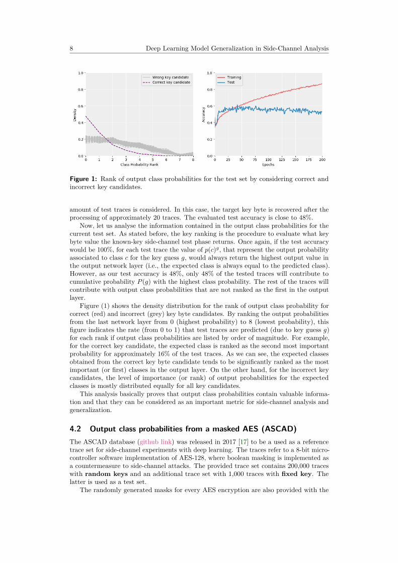
Figure 1: Rank of output class probabilities for the test set by considering correct andincorrect key candidates.

amount of test traces is considered. In this case, the target key byte is recovered after theprocessing of approximately 20 traces. The evaluated test accuracy is close to 48%.

Now, let us analyse the information contained in the output class probabilities for thecurrent test set. As stated before, the key ranking is the procedure to evaluate what keybyte value the known-key side-channel test phase returns. Once again, if the test accuracywould be 100%, for each test trace the value of p(c)g, that represent the output probabilityassociated to class c for the key guess g, would always return the highest output value inthe output network layer (i.e., the expected class is always equal to the predicted class).However, as our test accuracy is 48%, only 48% of the tested traces will contribute tocumulative probability P (g) with the highest class probability. The rest of the traces willcontribute with output class probabilities that are not ranked as the first in the outputlayer.

Figure (1) shows the density distribution for the rank of output class probability forcorrect (red) and incorrect (grey) key byte candidates. By ranking the output probabilitiesfrom the last network layer from 0 (highest probability) to 8 (lowest probability), thisfigure indicates the rate (from 0 to 1) that test traces are predicted (due to key guess g)for each rank if output class probabilities are listed by order of magnitude. For example,for the correct key candidate, the expected class is ranked as the second most importantprobability for approximately 16% of the test traces. As we can see, the expected classesobtained from the correct key byte candidate tends to be significantly ranked as the mostimportant (or first) classes in the output layer. On the other hand, for the incorrect keycandidates, the level of importance (or rank) of output probabilities for the expectedclasses is mostly distributed equally for all key candidates.

This analysis basically proves that output class probabilities contain valuable informa-tion and that they can be considered as an important metric for side-channel analysis andgeneralization.

4.2 Output class probabilities from a masked AES (ASCAD)The ASCAD database (github link) was released in 2017 [17] to be a used as a referencetrace set for side-channel experiments with deep learning. The traces refer to a 8-bit micro-controller software implementation of AES-128, where boolean masking is implemented asa countermeasure to side-channel attacks. The provided trace set contains 200,000 traceswith random keys and an additional trace set with 1,000 traces with fixed key. Thelatter is used as a test set.

The randomly generated masks for every AES encryption are also provided with the

Guilherme Perin 9

Figure 2: Rank of output class probabilities for the test set by considering correct andincorrect key candidates for ASCAD database.

database metadata. From these mask values, we could confirm that in the first encryptionround the intermediates associated to key bytes 0 and 1 are unprotected because the maskvalues that would generate a masked Sbox output byte value is set to zero for all traces.For the rest of key bytes, the remaining 14 mask bytes are random. Therefore, and to keepit simple, we decided to apply our analysis on the processing of key byte 2. For training,validation and test phases, the selected leakage model is Hamming weight of Sbox outputwithout the consideration of mask values and the knowledge of countermeasures (black-boxscenario).

The implemented neural network model is more complex if compared to the previousexample (Section 4.1). This time, we define a multiple layer perceptron with five hiddenlayers, where each layer contains 200 neurons and activation function Relu. The rest of thehyper-parameters are the same as the ones considered for the leaky AES in the previoussubsection.

Figure (2) shows the ranks for the output class probabilities for correct and incorrectkey candidates. Due to countermeasures, we can see that these probabilities are rankedsimilarly for all key candidates. However, it is slightly more concentrated as the mostimportant predicted classes for the correct key candidate (specially rank 2 which appearsmore for this correct key candidate). Our conclusion is that the model is being able togeneralize to the test data under the stipulated conditions for the side-channel analysis.

By simply observing the main metrics like accuracy in Figure 2, we are unable toidentify the generalization phase. In the current experiment, the test accuracy decreaseswith the processing of epochs. If we would have to identify the main training phases(underfitting, generalization or overfitting) from the accuracy metrics, we would assumethat the neural network model starts in a underfitting scenario (up to 25 epochs) and nextit starts to fit the training set until the overfitting scenario would be achieved if more epochswould be processed. From the test accuracy, we assume that the generalization phase neverhappened. Nevertheless, this is not what the rank of output class probabilities indicates andfor the side-channel problem the trained model provides good enough generalization. Thecorrect key byte can actually be recovered from this test and it can be distinguished fromoutput class probabilities. The cumulative probability therefore is a valid distinguisher forside-channel analysis with neural networks.

10 Deep Learning Model Generalization in Side-Channel Analysis

5 The meaning of generalization gap and validation met-rics in SCA

Generalization gap is well-known in the deep learning community because it explains thedifference between model’s performance on training data and unseen or test data. Asexplained in the previous section, output class probabilities, when ranked by order ofmagnitude according to key candidates, represents the generalization of a trained modelexpressed in terms of successful key recovery. In other words, if the model is generalizing,the output class probabilities for the correct key candidate will be concentrated as the firstones by order of magnitude, explaining the reason why a very low accuracy (sometimesslightly above the random guessing value) can be associated to a trained model that isable to recover the correct key candidate.

In [26], the authors propose a measure for predicting generalization gap, which isbased on the concept of margin distribution, i.e., distance of the training points to thedecision boundary, which is a concept used in support vector machines. In short, theauthors question how to predict the generalization gap based on training data and thenetwork parameters. Moreover, they propose a predictor with a high correlation betweenthe predicted and the real generalization gap. The motivation behind the work of [26]comes from the importance of predicting the gap between training and validation metricsin order to find ways of minimizing this gap and also to identify the main reasons forthe occurrence of this gap. In side-channel analysis, predicting the generalization gap isimportant for the understanding of how the trained model would be able to generalize toany test data and not only to the validation set that it is available during the known-keyanalysis scenario.

The original concept of generalization gap is restricted to the analysis on training andvalidation sets. In side-channel analysis, the generalization might be significantly low andindeed deep learning metrics sometimes cannot be used to represent the side-channel attackperformance (this is explained in more details in [16]). If the model is optimized for thevalidation set, there is still a big risk of misleading generalization for a separate test set.Therefore, to validate a model based on generalization gap may lead to inconsistent resultsin side-channel analysis. To sustain this last argument, in this section we conduct someexperiments to verify if the minimum gap between training and validation metrics leads togood levels of generalization.

In our methodology, several hyper-parameters configurations are defined for neuralnetworks (multiple layer perceptrons and convolutional neural networks) and the bestmodel is selected based on a metric. We start by checking the test performance (key rankand success rate) when the reference metrics are generalization gap based on accuracy,recall and loss values. The success rate represents the probability of recovering the keybyte for the processing of specific amount of traces.

5.1 Metrics for a leaky AESInitially, a leaky AES implementation is evaluated in order to compare the test performanceif generalization gap is a reference metric to select the best model. We train 10 differentneural networks with the same training data consisting of 2,000 traces. The validationset and test sets consist of 100 traces each. The process of training 10 different models iscalled a campaign and therefore the number of campaigns is 20. For each campaign, thebest trained model is selected from generalization gap metrics, which are: (1) different oftraining and validation accuracy, (2) difference of training and validation recall and (3)difference of training and validation loss. Figure 3 shows the averaged key rank computedfrom the key ranks from the best model of each campaign. Figure 4 shows the averagedkey rank from the 20 campaigns when only the validation metrics (accuracy, recall and

Guilherme Perin 11

loss) are used as a reference.

Figure 3: Key rank for test set of leaky AES: trained model selected from generalizationgap of metrics.

Figure 4: Key rank for test set of leaky AES: trained model selected from validationmetrics only.

Comparing Figures 3 and 4, we can conclude that validation metrics are a betteralternative than generalization gap for the validation of a trained model. As we can seein Figure 3, not all reference gap metrics lead to the selection of a best model from eachcampaign. Moreover, Figure 4 also provide the averaged key rank when the best models areselected when validation key rank is used as a reference validation metric. It is importantto mention that this is a very leaky target, and, for most of trained models, validationmetrics indicate a good level of generalization for side-channel analysis. This explainswhy, in Figure 4 all reference metrics result in a good test performance. Figures 5 and 6show the success rate for the 10 evaluated campaigns. Again, test results achieved fromvalidation metrics are slightly superior than the ones obtained from generalization gapmetrics. For the latter, the success rate achieves 100% with more test traces if comparedto the validation metrics case.

Figure 5: Success rate for test set of leaky AES: trained model selected from generalizationgap of metrics.

Now, the analysis of Figure 7 gives a graphical indication of how metrics obtainedfrom differences between training and validation (gap) and test metrics are related to each

12 Deep Learning Model Generalization in Side-Channel Analysis

Figure 6: Success rate for test set of leaky AES: trained model selected from validationmetrics only.

other. In this case, one would expect a negative correlation (i.e., lower the gap metric,higher the test metric). On the other hand, the results provided in 8 indicates a highcorrelation between validation and test metrics, which enforces why validation metricsare more relevant for conclusions about a trained model and, indeed, the prediction ofgeneralization in side-channel analysis.

Figure 7: Correlation between gap and validation metrics for leaky AES traces (200trained models = 20 campaigns × 10 models).

Figure 8: Correlation between test and validation metrics for leaky AES traces (200trained models = 20 campaigns × 10 models).

5.2 Metrics for masked AESThe key rank and success rate results obtained from a leaky AES indicate that anyvalidation metric is a good choice to define a neural network model among several modelswith different hyper-parameters. However, validation metrics (e.g. accuracy or recall)obtained from a model trained with side-channel traces measured from protected AESimplementations usually are close to a random guess. As a consequence, the generalizationgap (either based on accuracy or recall) might provide meaningless metrics. The sameprocedure applied to the leaky AES traces are now repeated for the masked AES tracesfrom ASCAD database, which is described in the previous section. Again, 10 differentmodels (with different hyper-parameters) are trained and this campaign is repeated 20times. The training set is composed of 50,000 traces. Figure 9 shows the final key ranks

Guilherme Perin 13

averaged over the best models selected for each one of the 20 campaigns. In this case, themodels are selected by having the generalization gap as a reference. Figure 10 providesthe averaged key rank results when best models are selected from validation metrics only.Additionally, this last figure also contains the averaged key rank when the best model ineach campaign is selected from the best final key rank result obtained from the validationset. The validation key rank calculation assumes a known-key scenario, i.e., validationtraces are collected from a device where the key is known or can be set by the adversary.

Figure 9: Key rank for test set of masked AES: trained model selected from generalizationgap of metrics.

Figure 10: Key rank for test set of masked AES: trained model selected from validationmetrics only.

Figure 11: Success rate for test set of masked AES: trained model selected from general-ization gap of metrics.

Not surprisingly, as illustrated by Figure 12, selecting the best model based on bestvalidation key rank per campaign as a validation metric leads to the best success rate aswell as the best averaged key rank in the test set, as shown in Figure 10. The key rank iscomputed from output class probabilities and due to the cumulative probability procedure,key rank appears to be a promising metric for validating a model. We reinforce that thisis the typical case where generalization (large generalization gap) is very limited due tonoise and countermeasures.

14 Deep Learning Model Generalization in Side-Channel Analysis

Figure 12: Success rate for test set of masked AES: trained model selected from validationmetrics only.

Figure 13 shows the correlation between gap and validation metrics for the experimentson the masked AES traces. The statistical relation between these two groups of metricsshows that test metrics (specially accuracy and recall) are not varying as the gap betweentraining and validation metrics vary. In other words, in a ideal scenario, one wouldexpect that the gap should be small and the test metrics should correspondent by growingproportionally. However, as mentioned before, the generalization of neural networks againstprotected targets is very limited and therefore the gap between training and validationmetrics is not a good reference for the validation of a model. On the other hand, validationmetrics only are highly correlated to the test metrics, even against protected AES. This canbe confirmed by observing the success rates in Figure 12. Despite the result with accuracy,recall and loss metrics from validation set only, the validation key rank resulted in thebest reference metric for selecting the best trained model for each one of the campaigns.

Figure 13: Correlation between gap and validation metrics for masked AES traces (200trained models = 20 campaigns × 10 models).

Figure 14: Correlation between test and validation metrics for masked AES traces (200trained models = 20 campaigns × 10 models).

6 Model ensembles for side-channel analysisEnsemble learning is a technique that combines the predictions from several models inorder to reduce the generalization error. The expected result is that the prediction obtainedfrom ensemble models is superior if compared to a single model. This is motivated bythe statistical intuition that averaging measurements (or predictions) can lead to a more

Guilherme Perin 15

stable and reliable estimate because we reduce the influence of random fluctuations insingle measurements.

Ideally, the hyper-parameters for each model should vary in order to learn differentfeatures from the same training set. If the models have equal configurations, it is verylikely that the neural network will learn similar representations from the training set andprovide similar classification results for the same test set. Another option, which we followin this paper, is to randomly split the training set into smaller sets and train a separatemodel for each one of them. In this case, the single models can have same structure.On the other hand, we can build an ensemble of slightly different models from the sametraining data, which can reduce the influence of random fluctuations in single models.

Here, the main goal of the ensemble learning application is to improve the distinguisha-bility of the cumulative probability (or output class probability ranks) in the key recoveryor test phase. When a deep learning-based side-channel attack is successful, the mainreason for that comes from the cumulative probability (Equation 1) being larger for thecorrect key candidate in the lower ranks (see for example Figure 1 where the lower ranksare more concentrated for the correct key candidate). As a result, successful ensemblesshould increase the cumulative probability for the correct key candidate while averagesout the variations for the incorrect candidates.

Note, however, that we are not assuming that ensemble learning is always better ifcompared to a single learning model. The main goal of this analysis is to demonstrate thatthe chances of success in terms of key recovery are higher for ensembles when comparedto single models. For a very large training set, one expects that a complex deep neuralnetwork needs to be defined. This actually requires a careful selection of hyper-parametersand to try each new configuration may takes a significant amount of time and computationpower. Ensemble learning makes use of smaller training sets, which reduces the complexityfor defining appropriate hyper-parameters. Moreover, because several models are combinedinto one, if few of the models contain hyper-parameters that does not provide goodlearnability from training sets, the fluctuations introduced by these models will be removedby having models that are actually generalizing. The experiments provided in this sectiondemonstrate that ensembles are more likely to succeed if compared to single learningmodels for a specific amount of trained models.

Ensemble learning methods do not exclude the importance of a correct hyper-parametersselection for each single model. The selection of these hyper-parameters can vary for eachmodel (heterogeneous) or remain the same (homogeneous). The idea of using heterogeneousmodels is the possible removal of errors imposed by the wrong selection of hyper-parametersif a sufficient amount of models is trained and if most of the neural networks are configuredwith reasonable hyper-parameters (i.e., hyper-parameters that provide a minimum levelof generalization). Hyper-parameters search methods, like random search, grid search,Bayesian optimization or genetic algorithms, also provide solutions to define the bestconfiguration for a neural network. However, these types of search would consider alarge training set and several iterations (e.g., the generations in the genetic algorithmsearch). This could render the analysis impractical due to computational or time contraints.Ensembles can work on smaller training sets and they require a limited amount of models,which reduces the complexity.

Main methods for ensemble learning include boosting, bagging and stacking. In thiswork, the implemented ensembles are more similar to bagging methodology. We decidedto use ensembles with averaged probabilities. The boosting and stacking methodswill be reserved for future works. Here, the applied method computes the new likelihoodfor each key candidate by averaging the probabilities from all the single models. Thecumulative probabilities from ensemble learning Pe(g) are then computed for each keybyte candidate g as follows:

16 Deep Learning Model Generalization in Side-Channel Analysis

Pe(g) =NM∑m=1

NT∑i=1

log(pm,i(c)g) (2)

In Eq. (2), the term NM refers to the number of single models. The term pm,i(c)g

refers to the output class probability c for model m and trace i according to key guess g.After building the ensembles, we expect an improvement in the key ranking convergencewhich, in the end, comes from the ensemble cumulative probabilities. The main goals ofthis analysis are:

• To verify the benefits of ensemble learning in side-channel analysis when ensemblesare built from all trained single models;

• To verify the benefits of ensemble learning in side-channel analysis when ensemblesare built from Nb best trained single models. The best models are selected basedon key rank for validation set, as this metric provided better results in the previoussection;

In the following, we conduct the analysis on leaky and masked AES traces.

6.1 Ensembles on a leaky AESAs an initial proof-of-concept, we firstly provide results for the unprotected AES case. Wetrain 10 models with a very small training set of 2,000 traces. The validation and test setscontain 200 traces each. The data sets are labelled according to the Hamming weight ofSbox output byte in the first AES round. The analysis and success rate are conducted forthe first key byte.

To compute the success rates, 40 campaigns with 10 single models each are executed.Ensembles are built from homogeneous and heterogeneous single models. For both cases,we set a weight initialization with random uniform method from Keras library, which inthe end will provide different trained models even if the same model is trained with thesame training data. The neural network topologies are multiple layer perceptron and thevaried hyper-parameters for heterogeneous models are: number of layers, units per layer,activation functions and learning rate.

Figure 15 shows the success rate for each single trained model and also for the resultingensemble models. As we can see, the ensemble models are at least good as electing abest model per campaign. For the heterogeneous case, the ensemble are slightly (but notmuch) superior than the best model. The fact that ensembles are not providing meaningfulimprovement is actually expected, mainly due to the presence of significant leakages thatcan be easily learned from different models.

6.2 Ensembles on a masked AESSide-channel traces from ASCAD database are again considered here in order to verifythe benefit of ensembles against masked AES implementations. For all the experimentsof this section, the training set contains random keys (as detailed in Section 4.2) andvalidation and test sets contain 500 traces each. The amount of training traces varies foreach experiment, as detailed in this section. Traces are labelled according to Hammingweight of Sbox output byte in the first AES round. Again, we consider the attack on onlyone key byte. We conduct the following tests with ensemble learning:

• Homogeneous case: Train 10 equal single models for different training set sizes.For each model, the training set is randomly selected out of 200,000 available trainingtraces. All single models are convolutional neural networks containing identicalhyper-parameters configuration.

Guilherme Perin 17

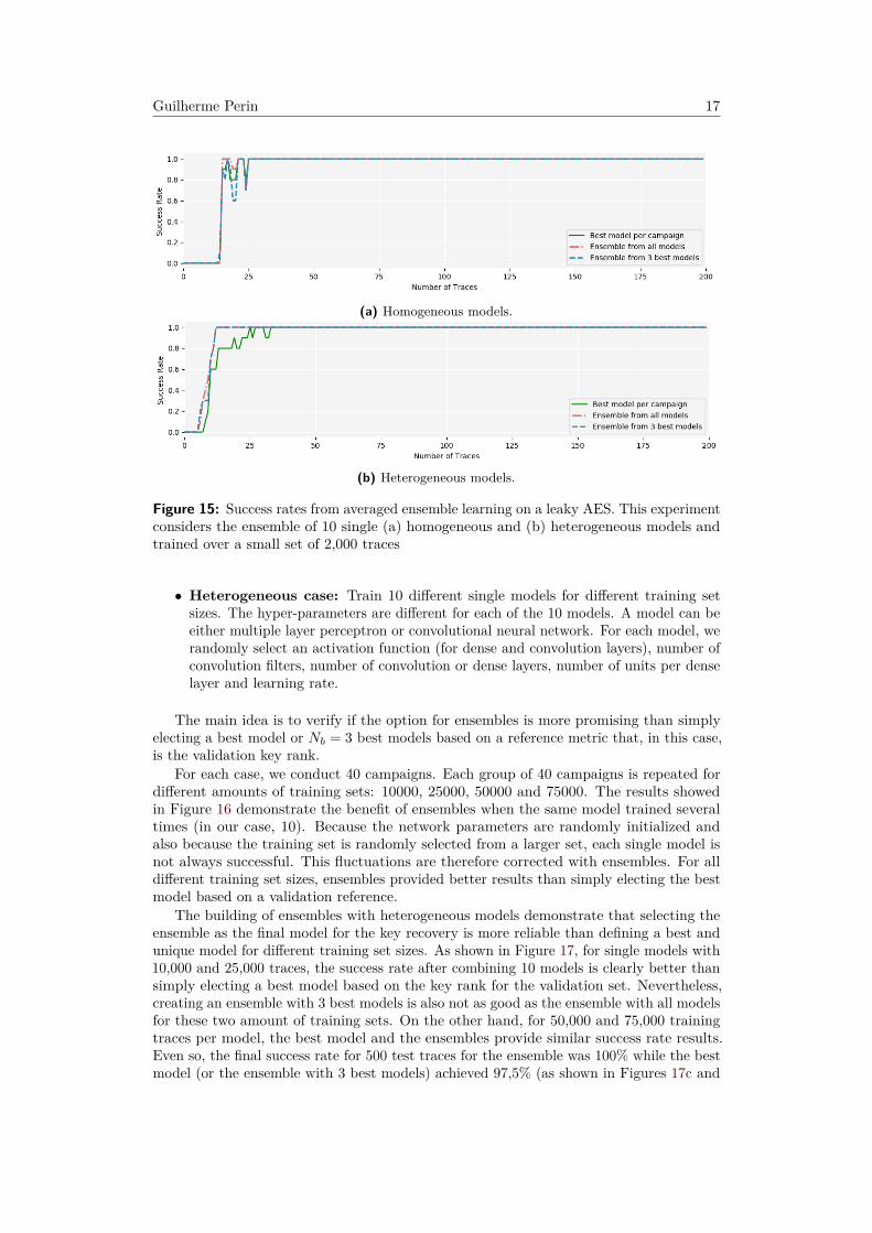
(a) Homogeneous models.

(b) Heterogeneous models.

Figure 15: Success rates from averaged ensemble learning on a leaky AES. This experimentconsiders the ensemble of 10 single (a) homogeneous and (b) heterogeneous models andtrained over a small set of 2,000 traces

• Heterogeneous case: Train 10 different single models for different training setsizes. The hyper-parameters are different for each of the 10 models. A model can beeither multiple layer perceptron or convolutional neural network. For each model, werandomly select an activation function (for dense and convolution layers), number ofconvolution filters, number of convolution or dense layers, number of units per denselayer and learning rate.

The main idea is to verify if the option for ensembles is more promising than simplyelecting a best model or Nb = 3 best models based on a reference metric that, in this case,is the validation key rank.

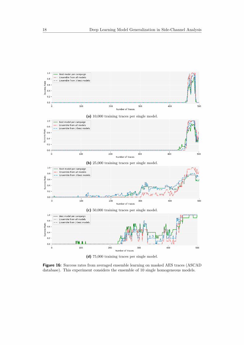
For each case, we conduct 40 campaigns. Each group of 40 campaigns is repeated fordifferent amounts of training sets: 10000, 25000, 50000 and 75000. The results showedin Figure 16 demonstrate the benefit of ensembles when the same model trained severaltimes (in our case, 10). Because the network parameters are randomly initialized andalso because the training set is randomly selected from a larger set, each single model isnot always successful. This fluctuations are therefore corrected with ensembles. For alldifferent training set sizes, ensembles provided better results than simply electing the bestmodel based on a validation reference.

The building of ensembles with heterogeneous models demonstrate that selecting theensemble as the final model for the key recovery is more reliable than defining a best andunique model for different training set sizes. As shown in Figure 17, for single models with10,000 and 25,000 traces, the success rate after combining 10 models is clearly better thansimply electing a best model based on the key rank for the validation set. Nevertheless,creating an ensemble with 3 best models is also not as good as the ensemble with all modelsfor these two amount of training sets. On the other hand, for 50,000 and 75,000 trainingtraces per model, the best model and the ensembles provide similar success rate results.Even so, the final success rate for 500 test traces for the ensemble was 100% while the bestmodel (or the ensemble with 3 best models) achieved 97,5% (as shown in Figures 17c and

18 Deep Learning Model Generalization in Side-Channel Analysis

(a) 10,000 training traces per single model.

(b) 25,000 training traces per single model.

(c) 50,000 training traces per single model.

(d) 75,000 training traces per single model.

Figure 16: Success rates from averaged ensemble learning on masked AES traces (ASCADdatabase). This experiment considers the ensemble of 10 single homogeneous models.

Guilherme Perin 19

(a) 10,000 training traces per single model.

(b) 25,000 training traces per single model.

(c) 50,000 training traces per single model.

(d) 75,000 training traces per single model.

Figure 17: Success rates from averaged ensemble learning on masked AES traces (ASCADdatabase). This experiment considers the ensemble of 10 single heterogeneous models.

20 Deep Learning Model Generalization in Side-Channel Analysis

17d). This confirms that defining an ensemble from all models is as good as selecting abest model from, e.g., hyper-parameters search. However, ensembles are not a replacementfor hyper-parameters search based on optimization algorithms. The usage of ensemblesensures more reliable results by eliminating the variance of different model results.

7 Conclusions and Future WorksThis paper proposed an analsyis of deep learning model generalization in side-channelanalysis. We provided an analysis of the output class probabilities from the test phase of adeep learning-based side-channel analysis. After reviewing the recent literature, we verifiedthat deep learning metrics are actually not completely aligned with side-channel metrics.We checked this argument with respect to test accuracy when the model is trained fromtraces measured from a masked AES implementation (ASCAD database). The resultsconfirmed that indeed test accuracy (and other deep learning metrics as recall or loss)usually does not translate the generalization of the trained model. The key ranking, in itsturn, is computed from output class probabilities. We graphically demonstrated how thecumulative probabilities in the key ranking calculation actually benefits not only from thehighest output class probability for each tested trace. With these results, we verified thereason why a relatively poor test accuracy, that would indicate underfitting or overfitting(which depends on the training metrics), can still result in a successful key recovery. To fillup the gap for a reference metric in order to define a best model for side-channel analysis,we verified that key rank for a fixed-key validation set leads to higher success rate results.

From the fact that output class probabilities are directly linked to the success of aside-channel analysis, we proposed the usage of ensemble learning by averaging the outputclass probabilities from several single models that may be trained with smaller trainingsets. The main conclusions from the use of ensembles in deep learning-based side-channelanalysis are:

• The ensembles are more likely to succeed in a side-channel test. After retraining thesame model with the hyper-parameters, we observed different key recovery results.The ensembles showed more stables results for different training set sizes;

• Ensembles are good alternatives for speeding up the training phase because it maybe successful on smaller training sets, as we could see in the previous section for thecase of deveral models trained with 25,000 traces. A single model was not successfulafter training on 25,000 traces.

• The use of ensembles relax the need of a careful selection of a strong group of hyper-parameters in neural networks. However, we do not conclude that ensembles replacehyper-parameter search algorithms. When a deep neural network is able to recoverthe key from masked AES implementations (as is the case of ASCAD dataset), notalways a selected group of hyper-parameters will be successful for smaller trainingsets. The ensembles demonstrated the ability of removing fluctuations from some ofthe models;

• We do not assume or conclude that ensembles improve the correct learnability ofneural networks from side-channel traces. If the model is configured and trained ina way that the generalization is very poor, it is very likely that ensembles will notimprove the generalization.

• The ensembles tend to provide a success rate that is at least good as the best singlemodel among several hyper-parameters configuration options. In our experiments,the ensembles always provided superior results.

Guilherme Perin 21

As mentioned in Section 6, ensembles are built with different methodologies. In thispaper, we considered the bagging methodology by averaging all and the best models.As future works, we propose to investigate other ensemble methodologies as boostingand stacking. Moreover, there is room to investigate the benefits of ensemble learningin combination with regularization techniques such as data augmentation and classicalregularizers (l1, l2 and dropout).

AcknowledgementsThis work was supported by the European Union’s H2020 Programme under grant agree-ment number ICT-731591 (REASSURE).

References[1] S. Chari, J. R. Rao, P. Rohatgi, Template attacks, in: B. S. K. Jr., Ç. K. Koç,

C. Paar (Eds.), Cryptographic Hardware and Embedded Systems - CHES 2002, 4thInternational Workshop, Redwood Shores, CA, USA, August 13-15, 2002, RevisedPapers, Vol. 2523 of Lecture Notes in Computer Science, Springer, 2002, pp. 13–28.doi:10.1007/3-540-36400-5\_3.URL https://doi.org/10.1007/3-540-36400-5_3

[2] W. Schindler, K. Lemke, C. Paar, A stochastic model for differential side channelcryptanalysis, in: J. R. Rao, B. Sunar (Eds.), Cryptographic Hardware and EmbeddedSystems - CHES 2005, 7th International Workshop, Edinburgh, UK, August 29 -September 1, 2005, Proceedings, Vol. 3659 of Lecture Notes in Computer Science,Springer, 2005, pp. 30–46. doi:10.1007/11545262\_3.URL https://doi.org/10.1007/11545262_3

[3] L. Lerman, S. F. Medeiros, G. Bontempi, O. Markowitch, A machine learning approachagainst a masked AES, in: Francillon and Rohatgi [27], pp. 61–75. doi:10.1007/978-3-319-08302-5\_5.URL https://doi.org/10.1007/978-3-319-08302-5_5

[4] Z. Martinasek, J. Hajny, L. Malina, Optimization of power analysis usingneural network, in: Francillon and Rohatgi [27], pp. 94–107. doi:10.1007/978-3-319-08302-5\_7.URL https://doi.org/10.1007/978-3-319-08302-5_7

[5] P. C. Kocher, J. Jaffe, B. Jun, Differential power analysis, in: M. J. Wiener (Ed.),Advances in Cryptology - CRYPTO ’99, 19th Annual International CryptologyConference, Santa Barbara, California, USA, August 15-19, 1999, Proceedings, Vol.1666 of Lecture Notes in Computer Science, Springer, 1999, pp. 388–397. doi:10.1007/3-540-48405-1\_25.URL https://doi.org/10.1007/3-540-48405-1_25

[6] E. Brier, C. Clavier, F. Olivier, Correlation power analysis with a leakage model, in:M. Joye, J. Quisquater (Eds.), Cryptographic Hardware and Embedded Systems -CHES 2004: 6th International Workshop Cambridge, MA, USA, August 11-13, 2004.Proceedings, Vol. 3156 of Lecture Notes in Computer Science, Springer, 2004, pp.16–29. doi:10.1007/978-3-540-28632-5\_2.URL https://doi.org/10.1007/978-3-540-28632-5_2

[7] B. Gierlichs, L. Batina, P. Tuyls, B. Preneel, Mutual information analysis, in: E. Os-wald, P. Rohatgi (Eds.), Cryptographic Hardware and Embedded Systems - CHES

22 Deep Learning Model Generalization in Side-Channel Analysis

2008, 10th International Workshop, Washington, D.C., USA, August 10-13, 2008.Proceedings, Vol. 5154 of Lecture Notes in Computer Science, Springer, 2008, pp.426–442. doi:10.1007/978-3-540-85053-3\_27.URL https://doi.org/10.1007/978-3-540-85053-3_27

[8] L. Batina, B. Gierlichs, K. Lemke-Rust, Differential cluster analysis, in: C. Clavier,K. Gaj (Eds.), Cryptographic Hardware and Embedded Systems - CHES 2009, 11thInternational Workshop, Lausanne, Switzerland, September 6-9, 2009, Proceedings,Vol. 5747 of Lecture Notes in Computer Science, Springer, 2009, pp. 112–127. doi:10.1007/978-3-642-04138-9\_9.URL https://doi.org/10.1007/978-3-642-04138-9_9

[9] H. Maghrebi, T. Portigliatti, E. Prouff, Breaking cryptographic implementations usingdeep learning techniques, in: C. Carlet, M. A. Hasan, V. Saraswat (Eds.), Security,Privacy, and Applied Cryptography Engineering - 6th International Conference,SPACE 2016, Hyderabad, India, December 14-18, 2016, Proceedings, Vol. 10076of Lecture Notes in Computer Science, Springer, 2016, pp. 3–26. doi:10.1007/978-3-319-49445-6\_1.URL https://doi.org/10.1007/978-3-319-49445-6_1

[10] E. Cagli, C. Dumas, E. Prouff, Convolutional neural networks with data augmentationagainst jitter-based countermeasures - profiling attacks without pre-processing, in:W. Fischer, N. Homma (Eds.), Cryptographic Hardware and Embedded Systems -CHES 2017 - 19th International Conference, Taipei, Taiwan, September 25-28, 2017,Proceedings, Vol. 10529 of Lecture Notes in Computer Science, Springer, 2017, pp.45–68. doi:10.1007/978-3-319-66787-4\_3.URL https://doi.org/10.1007/978-3-319-66787-4_3

[11] M. Carbone, V. Conin, M. Cornelie, F. Dassance, G. Dufresne, C. Dumas, E. Prouff,A. Venelli, Deep learning to evaluate secure RSA implementations, IACR Trans.Cryptogr. Hardw. Embed. Syst. 2019 (2) (2019) 132–161. doi:10.13154/tches.v2019.i2.132-161.URL https://doi.org/10.13154/tches.v2019.i2.132-161

[12] L. Masure, C. Dumas, E. Prouff, Gradient visualization for general characterizationin profiling attacks, in: I. Polian, M. Stöttinger (Eds.), Constructive Side-ChannelAnalysis and Secure Design - 10th International Workshop, COSADE 2019, Darmstadt,Germany, April 3-5, 2019, Proceedings, Vol. 11421 of Lecture Notes in ComputerScience, Springer, 2019, pp. 145–167. doi:10.1007/978-3-030-16350-1\_9.URL https://doi.org/10.1007/978-3-030-16350-1_9

[13] B. Hettwer, S. Gehrer, T. Güneysu, Deep neural network attribution methods forleakage analysis and symmetric key recovery, IACR Cryptology ePrint Archive 2019(2019) 143.URL https://eprint.iacr.org/2019/143

[14] G. Perin, B. Ege, L. Chmielewski, Neural network model assessment for side-channelanalysis, IACR Cryptology ePrint Archive 2019 (2019) 722.URL https://eprint.iacr.org/2019/722

[15] F. Wegener, T. Moos, A. Moradi, DL-LA: deep learning leakage assessment: A modernroadmap for SCA evaluations, IACR Cryptology ePrint Archive 2019 (2019) 505.URL https://eprint.iacr.org/2019/505

[16] S. Picek, A. Heuser, A. Jovic, S. Bhasin, F. Regazzoni, The curse of class imbalanceand conflicting metrics with machine learning for side-channel evaluations, IACR

Guilherme Perin 23

Trans. Cryptogr. Hardw. Embed. Syst. 2019 (1) (2019) 209–237. doi:10.13154/tches.v2019.i1.209-237.URL https://doi.org/10.13154/tches.v2019.i1.209-237

[17] E. Prouff, R. Strullu, R. Benadjila, E. Cagli, C. Dumas, Study of deep learningtechniques for side-channel analysis and introduction to ASCAD database, IACRCryptology ePrint Archive 2018 (2018) 53.URL http://eprint.iacr.org/2018/053

[18] L. Weissbart, S. Picek, L. Batina, One trace is all it takes: Machine learning-basedside-channel attack on eddsa, IACR Cryptology ePrint Archive 2019 (2019) 358.URL https://eprint.iacr.org/2019/358

[19] H. Maghrebi, Deep learning based side channel attacks in practice, IACR CryptologyePrint Archive 2019 (2019) 578.URL https://eprint.iacr.org/2019/578

[20] J. Kim, S. Picek, A. Heuser, S. Bhasin, A. Hanjalic, Make some noise. unleashingthe power of convolutional neural networks for profiled side-channel analysis, IACRTrans. Cryptogr. Hardw. Embed. Syst. 2019 (3) (2019) 148–179. doi:10.13154/tches.v2019.i3.148-179.URL https://doi.org/10.13154/tches.v2019.i3.148-179

[21] Y. Zhou, F.-X. Standaert, Deep learning mitigates but does not annihilate the needof aligned traces and a generalized resnet model for side-channel attacks, Journal ofCryptographic Engineeringdoi:10.1007/s13389-019-00209-3.

[22] G. Yang, H. Li, J. Ming, Y. Zhou, Convolutional neural network based side-channelattacks in time-frequency representations, in: B. Bilgin, J. Fischer (Eds.), SmartCard Research and Advanced Applications, 17th International Conference, CARDIS2018, Montpellier, France, November 12-14, 2018, Revised Selected Papers., Vol.11389 of Lecture Notes in Computer Science, Springer, 2018, pp. 1–17. doi:10.1007/978-3-030-15462-2\_1.URL https://doi.org/10.1007/978-3-030-15462-2_1

[23] B. Hettwer, S. Gehrer, T. Güneysu, Profiled power analysis attacks using convolutionalneural networks with domain knowledge, in: C. Cid, M. J. J. Jr. (Eds.), Selected Areasin Cryptography - SAC 2018 - 25th International Conference, Calgary, AB, Canada,August 15-17, 2018, Revised Selected Papers, Vol. 11349 of Lecture Notes in ComputerScience, Springer, 2018, pp. 479–498. doi:10.1007/978-3-030-10970-7\_22.URL https://doi.org/10.1007/978-3-030-10970-7_22

[24] B. Timon, Non-profiled deep learning-based side-channel attacks with sensitivityanalysis, IACR Trans. Cryptogr. Hardw. Embed. Syst. 2019 (2) (2019) 107–131.doi:10.13154/tches.v2019.i2.107-131.URL https://doi.org/10.13154/tches.v2019.i2.107-131

[25] L. Masure, C. Dumas, E. Prouff, A comprehensive study of deep learning for side-channel analysis, IACR Cryptology ePrint Archive 2019 (2019) 439.URL https://eprint.iacr.org/2019/439

[26] Y. Jiang, D. Krishnan, H. Mobahi, S. Bengio, Predicting the generalization gap indeep networks with margin distributions, in: 7th International Conference on LearningRepresentations, ICLR 2019, New Orleans, LA, USA, May 6-9, 2019, OpenReview.net,2019.URL https://openreview.net/forum?id=HJlQfnCqKX

24 Deep Learning Model Generalization in Side-Channel Analysis

[27] A. Francillon, P. Rohatgi (Eds.), Smart Card Research and Advanced Applications -12th International Conference, CARDIS 2013, Berlin, Germany, November 27-29, 2013.Revised Selected Papers, Vol. 8419 of Lecture Notes in Computer Science, Springer,2014. doi:10.1007/978-3-319-08302-5.URL https://doi.org/10.1007/978-3-319-08302-5