1

Deep Learning on Sparse Manifolds for FasterObject Segmentation

Jacinto C. Nascimento∗, Member, IEEE, Gustavo Carneiro

Abstract— We propose a new combination of deep beliefnetworks and sparse manifold learning strategies for the 2Dsegmentation of non-rigid visual objects. With this novel com-bination, we aim to reduce the training and inference com-plexities while maintaining the accuracy of machine learningbased non-rigid segmentation methodologies. Typical non-rigidobject segmentation methodologies divide the problem into a rigiddetection followed by a non-rigid segmentation, where the lowdimensionality of the rigid detection allows for a robust training(i.e., a training that does not require a vast amount of annotatedimages to estimate robust appearance and shape models) and afast search process during inference. Therefore, it is desirable thatthe dimensionality of this rigid transformation space is as smallas possible in order to enhance the advantages brought by theaforementioned division of the problem. In this paper, we proposethe use of sparse manifolds to reduce the dimensionality of therigid detection space. Furthermore, we propose the use of deepbelief networks to allow for a training process that can producerobust appearance models without the need of large annotatedtraining sets. We test our approach in the segmentation of theleft ventricle of the heart from ultrasound images and lips fromfrontal face images. Our experiments show that the use of sparsemanifolds and deep belief networks for the rigid detection stageleads to segmentation results that are as accurate as the currentstate of the art, but with lower search complexity and trainingprocesses that require a small amount of annotated training data.

I. INTRODUCTION

Current methodologies for top-down segmentation of de-formable objects using machine learning techniques addressthe learning and inference tasks with a coarse-to-fine strategybased on the following two consecutive stages [1]–[6]: (i) rigiddetection and (ii) non-rigid segmentation. The rigid detection(i.e., coarse step) produces the rotation, scale and translation ofthe visual object, which are used to initialize and constrain thenon-rigid segmentation stage (i.e., fine step). Assuming thatthe contour of the visual object is represented by S keypoints(or S 2-D points) and the rigid detection is performed in aspace with R << 2S dimensions, then the introduction ofthis coarse step allows for a more efficient inference and lesscomplex training processes.

The improvement in the inference process efficiency stemsfrom the following two facts: 1) faster search in theR-dimensional rigid space (compared to the original S-dimensional non-rigid space) because of the much smaller

This work was supported by the FCT project [PEst-OE/EEI/LA0009/2013] and project ’SPARSIS’ - PTDC/EEIPRO/0426/2014.This work was also partially supported by the Australian Research Council’sDiscovery Projects funding scheme (project DP140102794).

Jacinto C. Nascimento (corresponding author) is with the Instituto deSistemas e Robotica, Instituto Superior Tecnico, 1049-001 Lisboa, Portu-gal. Email: jan@isr.ist.utl.pt. Phone: +351-218418270, Fax: +351-218418291.

dimensionality of R; and 2) efficient fine step in the 2S-dimensional non-rigid space given the initial guess and con-straint produced by the rigid detection step (see Fig. 1).The smaller training complexity is achieved because theR-dimensional rigid problem requires smaller training setsand the training for the non-rigid segmentation in the 2S-dimensional space is also simplified because of the constraintsproduced by the rigid detection stage. Note however, that thisstrategy imposes strong requirements on the rigid detector, inthe sense that it has to be efficient and robust to the appearanceand shape variations of the visual object of interest and thesize of the training set. The efficiency of this detector dependsmainly on the dimensionality of the rigid search space (i.e.,lower dimensionality leads to more efficient rigid detectors)and robustness also depends on this dimensionality (for effec-tively modeling the shape variations), but also depends on theability of the classifier to model the appearance of the objectusing a limited number of annotated images. It is importantto note that the usual solution to increase the robustness ofthe classifier when the number of annotated images is smallis to increase the training set by artificially perturbing thesetraining images and annotations (e.g., by adding image noiseor applying small rigid transformations) in order to generatenew images to be added to the training set. However, giventhe random nature of this perturbation, it is not possible toguarantee whether the generated image can actually exist inpractice, which ultimately can lead to ineffective classificationproblems.

This paper introduces a rigid search space of very lowdimensionality with the use of sparse manifolds, where theproblem of classifier robustness is dealt with the use of deeplearning mechanisms, which has shown unique robustnessparticularly with respect to the size of training set. Morespecifically, we propose the use of sparse manifolds with lowintrinsic dimensionality for the rigid detection stage [1,2,5]–[7], which allows for a faster inference process that producescompetitive segmentation results. Another aspect of our frame-work, is that by restricting the positive and negative samplesto lie in the learned low-dimensional sparse manifold, it ispossible to reduce significantly the need for additional artificialpositive and negative samples during the training process, andat the same time guarantee that the additional samples aremore likely to exist in practice. Consequently, this producesa less complex and faster training process that is as robust toshape and appearance variations as the current state of the art.

We illustrate the performance of the proposed low-dimensional rigid search space using sparse manifolds ap-proach in two different segmentation problems: the left ventri-cle (LV) endocardium segmentation from ultrasound (US) im-

2

(a) State-of-the-art coarse-to-fine search strategy

(b) Proposed coarse search using sparse manifolds in the rigid detection

Fig. 1. (a) Illustration of the two-stage strategy for the non-rigid segmentation used in the state-of-the-art methodologies. (b) Proposed methodology, wherethe sparse manifold is used in the rigid detection step.

agery and lip segmentation using the extended Cohn-Kanadedataset (CK+) [8] consisting of several facial expressions fromfrontal views. Note that all datasets presented in the papershare the conditions where the object of interest undergoesa rigid transformation followed by a non-rigid deformation.Also note that we are interested in segmenting the object usingan explicit representation, where neighboring keypoints in thesegmentation are strongly correlated.

We demonstrate that our framework reduces the searchcomplexity without a negative impact on the segmentationaccuracy, when compared to the state of the art. Moreover,we also show that the our proposed low-dimensional sparsemanifolds allows for the use of smaller training sets than thecurrent state-of-the-art methods.

II. LITERATURE REVIEW

The segmentation of non-rigid visual objects is perhaps oneof the most studied problems in the field of computer vision.In this literature review, we classify the proposed methodolo-gies as follows: bottom-up approaches [9,10], active contourmethods [11]–[23], deformable templates [24]–[29], and data-driven segmentation [6,30]–[48]. The vast majority of the thesemethodologies breaks down the non-rigid segmentation intotwo sub-problems, comprising a first stage that selects thelocation (and usually the scale and orientation too) of thesought visual object, followed by a second stage that searchesfor the boundary of the object given the information producedin the first stage. We call such methodologies coarse-to-fine,where the coarse step consists of the rigid detector and thefine stage comprises the constrained non-rigid segmentation,as explained in Section I. Recently, the non-rigid segmentationproblem has avoided the coarse stage altogether by addressingthe task either as a structured learning and inference problem[49,50] or as a convex active contour method [13]. In thestructured inference problem the input image is represented

with a graph combining multiple bottom-up and top-downfunctions; while in convex active contour methods, the mainidea is to convexify the level set energy function, which meansthat it no longer depends on the initial guess provided by thecoarse stage.

Classic bottom-up methods [9,10] are based on a coarse-to-fine methodology, where the coarse step is usually representedwith a manual initialization, which is followed by a seriesof standard image processing techniques to detect the borderof the sought object. In general, these image processingtechniques only take into account low-level image information,such as edges, texture and colour, and use simple priorinformation, such as boundary smoothness and continuity. Thesimplicity of the techniques make these approaches attractivefrom a computational complexity point of view, but the lackof high-level information about the visual object and thedependence on a good initialization (from the coarse step)make these approaches too sensitive to imaging conditions andto the appearance and shape variations of the sought visualobject.

Active contour methods [17] improved the robustness ofsegmentation algorithms to imaging conditions and to thevariations of the visual object by formulating the problemwith a unified energy function that could be minimized withstandard optimization methods. The development of level-set methods [20] improved the performance of active con-tours with respect to imaging conditions and visual objecttopology. We refer to such methods as coarse-to-fine non-convex active contours, since their energy function is notconvex, and depends strongly on good initial conditions thatare usually provided manually during the coarse step. Thelatest developments of these approaches have been focused onincreasing the robustness of the method with the integrationof region and boundary segmentation, reduction of the searchdimensionality, modeling of the implicit segmentation function

3

with a continuous parametric function, and the introduction ofshape and texture priors [11,12,14]–[16,18,19,21]–[23]. Theconvexification of the energy function used in active contourmethods has been a central topic of research in the field [13],which allows for more efficient optimization methods inaddition to the lack of need of manual initialization (i.e., thecoarse step is no longer needed). Nevertheless, these convexactive contour methods can only avoid the coarse search stepwhen the visual object of interest has strong priors in termsof texture, shape and rigid transform, which may not be thecase for some examples (see Fig. 2-a) and the search processwill not be able to extend much from these priors. Deformabletemplates [24]–[29] introduce the use of more specific priormodels about the shape and appearance of the visual objectof interest with the goal of deforming this prior model tomatch the test image. Similarly to the case of non-convexlevel sets, this approach also needs a coarse step comprisinga good initialization for the optimization process. Level-setsand deformable templates are among the most successfultechniques applied in non-rigid segmentation problems, buttheir main weakness is the strong prior knowledge defined inthe optimization function, such as the definition of the objectborder, the prior shape, the prior distribution of the texture orgray values, or the shape variation. This prior knowledge canbe either designed by hand or learned using a (usually) smalltraining set. As a result, the effectiveness of such approachesis limited by the validity of these prior models, which areunlikely to capture all possible shape variations and nuancespresent in the imaging of the visual object [37].

These issues are the main motivation of data-driven binarysegmentation methods, where the shape and appearance ofthe LV is fully learned from a manually annotated trainingset. Active shape and appearance models [31]–[33,39] areusually based on optimization methods of an energy func-tional composed of shape and appearance terms, representedby generative classifiers learned using a manually annotatedtraining set. The use of discriminative classifiers has also beenexplored in data-driven binary segmentation methods [6,37].The commonality between these two approaches is the use ofa coarse-to-fine search, with the coarse stage represented by asearch for the rigid transform of the mean shape of the soughtvisual object, which is followed by a fine stage that transformsthe mean shape in a non-rigid way to match visual object in thetest image. In general, the coarse stage must efficiently providea precise rigid transformation, so there has been a large numberof papers about effective coarse search strategies. Exploringthe whole rigid transform space is in general intractable, so themain idea is to progressively constrain this search space. Thecascade classifier [51] does that by firstly exploring the entiresearch space with highly robust low-complexity classifiers, andthen further testing the regions that survived that previous stepswith increasingly more complex classifiers. A similar approachis followed in [52], that imposes a prior distribution on theinitial search space, which is used to sample the initial searchlocations that are refined based on a gradient-based search.Another related approach is the marginal space learning [41],which partitions the search space into sub-spaces of increasingdimension and complexity. The branch and bound approach

for the coarse search step [53] is another way to progressivelyreducing the complexity of the search space.

The recent development of structured learning and inferencemethods [49,50] allowed the design of convex data-driven bi-nary [30,38] and multi-class [42]–[48] segmentation methods.The main potential advantage of such approaches lies in theirability to avoid the coarse search step because the structuredinference is designed as a convex problem independent of theinitial guess. However, as explained above for convex levelset methods, this advantage can be realized only if the visualobject of interest can be reasonably characterized by strongpriors in terms of appearance, shape, rigid transformation, etc.An alternative usually followed by state-of-the-art structuredinference and learning methods is the integration of the resultof coarse visual object detectors into the framework, whicheffectively means that most of the methods above run a coarsesearch step.

Another relevant point of our proposal, is the gradient basedsearch in manifolds, which have also been studied in otherworks. For instance, Helmke et al. [54] have introduced a newoptimization approach for the essential matrix computationwith the use of Gauss-Newton iterations. Huper et al. [55]also propose a numerical optimization of a cost functiondefined on a manifold. Similarly, the use of Newton’s methodalong the geodesics and variants of projections have also beenproposed by other authors [56]–[58]. Our approach representsan application of such gradient-based search methods in theproblem of top-down non-rigid segmentation with the specificgoals of reducing the search running time and the trainingcomplexity.

Finally, sparse manifold learning is another topic visited byour proposal. This basically involves the estimation of a low-dimensional representation of a data set using a small numberof observations [59,60]. One popular technique for finding asparse representation is the Matching Pursuit (MP), which isbased on a suboptimal forward sequential algorithms [61]–[64]. Other techniques are based on optimization methodolo-gies that maximize sparsity, such as the ℓ1 norm [65,66], orthe more general ℓ(ρ≤1) explored by FOCal UnderdeterminedSystem Solver (FOCUSS). Techniques tailored to be appliedin the context of noisy data have also been proposed, such asa robust version of the FOCUSS algorithm, called RegularizedFOCUSS, that can also be used as an efficient representationfor compression [67]. Other important variation of the sparselinear inverse problem is the multiple-measurement vector(MMV) that achieves sparse representations from single-measurement vectors (SMVs) [68]. Recent theoretical studiesfocus on the convex relaxation of the MMV such as theapproach based on the (ℓ2,ℓ1) norm minimization [60,69]–[71].A similar relaxation technique (via the ℓ1 norm minimization)is employed in the SMV model, but efficient MMV methodsfor sparse representation have been proposed, in which someknown results of SMV are generalized to MMV. The sparsemanifold learning proposed in this paper is inspired on ourprevious work [72], which introduces a manifold learningmethod that requires a large number of samples that leads toan inference lacking efficiency because each sample wouldneed to be used as an initial guess to a gradient-based

4

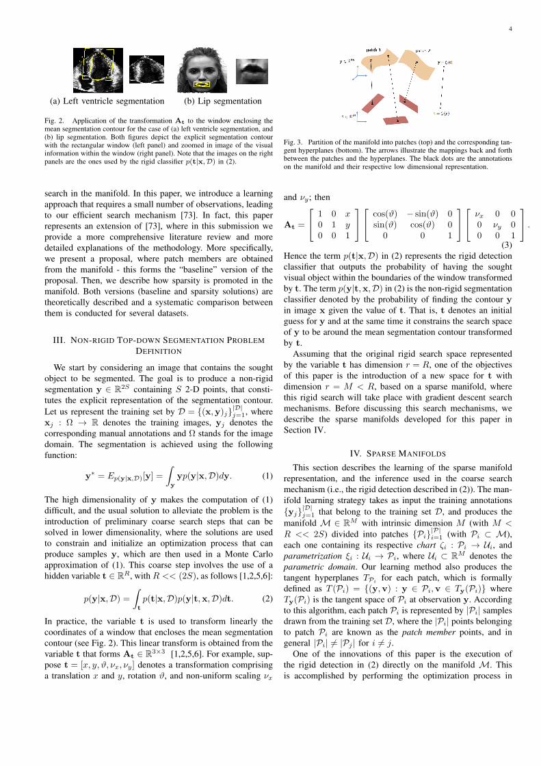
(a) Left ventricle segmentation (b) Lip segmentation

Fig. 2. Application of the transformation At to the window enclosing themean segmentation contour for the case of (a) left ventricle segmentation, and(b) lip segmentation. Both figures depict the explicit segmentation contourwith the rectangular window (left panel) and zoomed in image of the visualinformation within the window (right panel). Note that the images on the rightpanels are the ones used by the rigid classifier p(t|x,D) in (2).

search in the manifold. In this paper, we introduce a learningapproach that requires a small number of observations, leadingto our efficient search mechanism [73]. In fact, this paperrepresents an extension of [73], where in this submission weprovide a more comprehensive literature review and moredetailed explanations of the methodology. More specifically,we present a proposal, where patch members are obtainedfrom the manifold - this forms the “baseline” version of theproposal. Then, we describe how sparsity is promoted in themanifold. Both versions (baseline and sparsity solutions) aretheoretically described and a systematic comparison betweenthem is conducted for several datasets.

III. NON-RIGID TOP-DOWN SEGMENTATION PROBLEMDEFINITION

We start by considering an image that contains the soughtobject to be segmented. The goal is to produce a non-rigidsegmentation y ∈ R2S containing S 2-D points, that consti-tutes the explicit representation of the segmentation contour.Let us represent the training set by D = (x,y)j|D|j=1, wherexj : Ω → R denotes the training images, yj denotes thecorresponding manual annotations and Ω stands for the imagedomain. The segmentation is achieved using the followingfunction:

y∗ = Ep(y|x,D)[y] =

∫y

yp(y|x,D)dy. (1)

The high dimensionality of y makes the computation of (1)difficult, and the usual solution to alleviate the problem is theintroduction of preliminary coarse search steps that can besolved in lower dimensionality, where the solutions are usedto constrain and initialize an optimization process that canproduce samples y, which are then used in a Monte Carloapproximation of (1). This coarse step involves the use of ahidden variable t ∈ RR, with R << (2S), as follows [1,2,5,6]:

p(y|x,D) =

∫t

p(t|x,D)p(y|t,x,D)dt. (2)

In practice, the variable t is used to transform linearly thecoordinates of a window that encloses the mean segmentationcontour (see Fig. 2). This linear transform is obtained from thevariable t that forms At ∈ R3×3 [1,2,5,6]. For example, sup-pose t = [x, y, ϑ, νx, νy] denotes a transformation comprisinga translation x and y, rotation ϑ, and non-uniform scaling νx

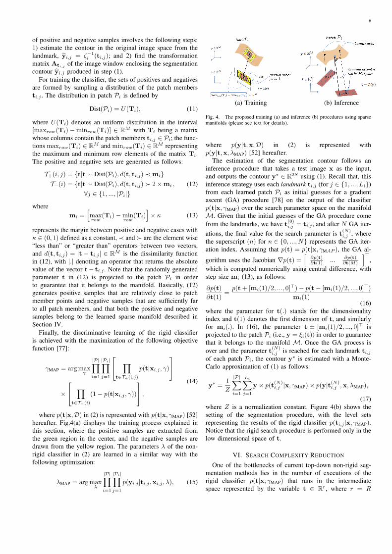
Fig. 3. Partition of the manifold into patches (top) and the corresponding tan-gent hyperplanes (bottom). The arrows illustrate the mappings back and forthbetween the patches and the hyperplanes. The black dots are the annotationson the manifold and their respective low dimensional representation.

and νy; then

At =

1 0 x0 1 y0 0 1

cos(ϑ) − sin(ϑ) 0sin(ϑ) cos(ϑ) 0

0 0 1

νx 0 00 νy 00 0 1

.

(3)Hence the term p(t|x,D) in (2) represents the rigid detectionclassifier that outputs the probability of having the soughtvisual object within the boundaries of the window transformedby t. The term p(y|t,x,D) in (2) is the non-rigid segmentationclassifier denoted by the probability of finding the contour yin image x given the value of t. That is, t denotes an initialguess for y and at the same time it constrains the search spaceof y to be around the mean segmentation contour transformedby t.

Assuming that the original rigid search space representedby the variable t has dimension r = R, one of the objectivesof this paper is the introduction of a new space for t withdimension r = M < R, based on a sparse manifold, wherethis rigid search will take place with gradient descent searchmechanisms. Before discussing this search mechanisms, wedescribe the sparse manifolds developed for this paper inSection IV.

IV. SPARSE MANIFOLDS

This section describes the learning of the sparse manifoldrepresentation, and the inference used in the coarse searchmechanism (i.e., the rigid detection described in (2)). The man-ifold learning strategy takes as input the training annotationsyj|D|j=1 that belong to the training set D, and produces themanifold M ∈ RM with intrinsic dimension M (with M <R << 2S) divided into patches Pi|P|i=1 (with Pi ⊂ M),each one containing its respective chart ζi : Pi → Ui, andparametrization ξi : Ui → Pi, where Ui ⊂ RM denotes theparametric domain. Our learning method also produces thetangent hyperplanes TPi for each patch, which is formallydefined as T (Pi) = (y,v) : y ∈ Pi,v ∈ Ty(Pi) whereTy(Pi) is the tangent space of Pi at observation y. Accordingto this algorithm, each patch Pi is represented by |Pi| samplesdrawn from the training set D, where the |Pi| points belongingto patch Pi are known as the patch member points, and ingeneral |Pi| = |Pj | for i = j.

One of the innovations of this paper is the execution ofthe rigid detection in (2) directly on the manifold M. Thisis accomplished by performing the optimization process in

5

each of the low dimensional patches Pi with initial guesses(for the segmentation process in (2)) taken from the patchmember points ti,j = ζi(yi,j), for i ∈ 1, ..., |P| and j ∈1, ..., |Pi|. Consequently, the efficiency of the segmentationdepends on a low number of patch member points in eachpatch. For completeness of the exposition, we provide detailsof the manifold learning algorithm in the Appendix.

A. Subset Selection - Problem Statement1

In order to reduce the number of patch member points ineach patch Pi, let us first arrange the training annotations inthe following matrix Yi ∈ R2S×|Pi| (each column containinga contour), with

Yi = [yi,1, ...,yi,|Pi|], (4)

where the charting process generates the matrix Ti =[ti,1, ..., ti,|Pi|] with Ti ∈ RM×|Pi|, i.e. the low dimensionalrepresentations of the annotations. The reduction in the numberof patch member points involves the selection of a smallnumber of columns in Yi (and thus a subset of columns inTi) to be used as landmarks. These columns are selected byminimizing the amount of information lost with respect to ζi,but note that preserving the chart ζi is equivalent to preserve itsinverse mapping, i.e. the parameterization ξi, which is morepractical to use since we can use the following generativemodel

yi,j = ξi(ti,j) + ω, (5)

where yi,j is an approximation of yi,j and ω is a Gaussianrandom variable representing noise. Our main goal in thiscontext is to design a method that estimates the fewest numberof landmarks so that yi,j is reliably approximated by yi,j in(5).

B. Linear regression

To accomplish the goal formulated above in Sec. IV-A, westart by building the radial basis function (RBF) kernel matrixK, with each of its elements represented by k(ti,l, ti,q) =exp(−∥ti,l − ti,q∥2/2σK) and reformulate (5) as a singlemeasurement vector problem (SMV) [73,74], as follows2

θ = Kβ + η, (6)

where θ ∈ R|Pi| represents the vector containing the maxi-mum principal angle between the tangent bundles Tyi,j andTPi [75] 3, β ∈ R|Pi| denotes the vector of coefficients forreconstructing the input data θ, and η ∈ R|Pi| is a randomvariable representing the additive Gaussian noise process.

An interpretation of the regression in (6) is that β preservesangular information within a patch, using a small number of

1All the exposition formulated in this Sections IV-A, IV-B, IV-C, are interms of the ith patch, being the same strategy applied to other patches inthe manifold.

2In the following equations (6),(7), (9), and (10) we have omitted thesubscript i for simplifying the notation.

3See the Appendix for additional details regarding the computation ofprincipal angle. Also, note that Tyi,j is the tangent subspace of yi,j (the jthcolumn of Y in (4)) and TPi

is the tangent subspace computed in the seedpoint of the ith patch.

points, and K preserves information regarding the distancebetween points. Thus, points with similar angular or distanceinformation are included in the regression.

C. Sparsity with Least Angle Regression

In order to select a small subset of the patch member pointsof Pi given θ, we estimate β in (6), denoted by β, constrainingit to be sparse via a regularization term. More specifically, theestimate β can be found by minimizing the following expectedgeneralization error

E(β) =∥∥θ −Kβ

∥∥2, (7)

defining the absolute norm of β as T (β) =∑|Pi|

j=1 |βj |, theminimization of E(β) subject to a bound t on T (β) can besolved as follows

minimize E(β) subject to T (β) ≤ t, (8)

which is solved with least angle regression (LARS) [76].Basically, the algorithm starts with the zero vector, β = 0,and adds covariates (i.e., the columns of K) to the model inaccordance to their correlation with the prediction error vector,∥θ−Kβ∥2 in (7), setting the corresponding jth entry, βj , toa value such that another covariate becomes equally correlatedwith the error and is, itself, added to the model. The LARSalgorithm then proceeds in a direction equiangular to all theadded βj and the process is repeated until all covariates havebeen added. This strategy of adding a new βj (making it non-zero), requires an amount of m steps (each step adding a newβj and making it non-zero). It has been shown [76] that therisk (i.e. the structural risk equivalent to the expected error in(7)) can be estimated as

R(βp) = ∥θ −Kβ∥∥2/σ2

θ −m+ 2p. (9)

where σθ can be computed from the unconstrained leastsquares solution of (6), m is the number of steps (i.e. di-mension of θ) and p is the number of non-zero entries of βj .

The landmarks are the columns ti,j of Ti (or equivalentlyof Yi) with the same indexes j as the non-zero elements ofβp such that

p∗ = argminp

(R(βp)). (10)

The estimated Li = p∗ landmarks correspond to p∗ non-zeroelements in βp. This strategy ensures that the landmarks arethe kernel centers that minimize the risk of the regressionformulated in (6).

V. TRAINING AND INFERENCE ON THE SPARSE MANIFOLDUSING DEEP BELIEF NETWORKS

The rigid detection classifier in (2) is modeled by theparameter vector γMAP (learned with a maximum a posteriorilearning algorithm), which means that p(t|x,D) is hereafterrepresented by p(t|x, γMAP). The parameter vector γMAP isestimated using a set of training samples taken from thepatch member points ti,j = ζi(yi,j) (for j ∈ 1, ..., |Pi|)of each learned patch Pi (for i ∈ 1, ..., |P|) produced bythe manifold learning algorithm. Specifically, the generation

6

of positive and negative samples involves the following steps:1) estimate the contour in the original image space from thelandmark, yi,j = ζ−1i (ti,j); and 2) find the transformationmatrix Ati,j of the image window enclosing the segmentationcontour yi,j produced in step (1).

For training the classifier, the sets of positives and negativesare formed by sampling a distribution of the patch membersti,j . The distribution in patch Pi is defined by

Dist(Pi) = U(Ti), (11)

where U(Ti) denotes an uniform distribution in the interval[maxrow(Ti)−minrow(Ti)] ∈ RM with Ti being a matrixwhose columns contain the patch members ti,j ∈ Pi; the func-tions maxrow(Ti) ∈ RM and minrow(Ti) ∈ RM representingthe maximum and minimum row elements of the matrix Ti.The positive and negative sets are generated as follows:

T+(i, j) = t|t ∼ Dist(Pi), d(t, ti,j) ≺ miT−(i) = t|t ∼ Dist(Pi), d(t, ti,j) ≻ 2×mi

∀j ∈ 1, ..., |Pi|, (12)

wheremi =

[maxrow

(Ti)−minrow

(Ti)]× κ (13)

represents the margin between positive and negative cases withκ ∈ (0, 1) defined as a constant, ≺ and ≻ are the element wise“less than” or “greater than” operators between two vectors,and d(t, ti,j) = |t − ti,j | ∈ RM is the dissimilarity functionin (12), with |.| denoting an operator that returns the absolutevalue of the vector t− ti,j . Note that the randomly generatedparameter t in (12) is projected to the patch Pi in orderto guarantee that it belongs to the manifold. Basically, (12)generates positive samples that are relatively close to patchmember points and negative samples that are sufficiently farto all patch members, and that both the positive and negativesamples belong to the learned sparse manifold described inSection IV.

Finally, the discriminative learning of the rigid classifieris achieved with the maximization of the following objectivefunction [77]:

γMAP = argmaxγ

|P|∏i=1

|Pi|∏j=1

∏t∈T+(i,j)

p(t|xi,j , γ)

×

∏t∈T−(i)

(1− p(t|xi,j , γ))

,

(14)

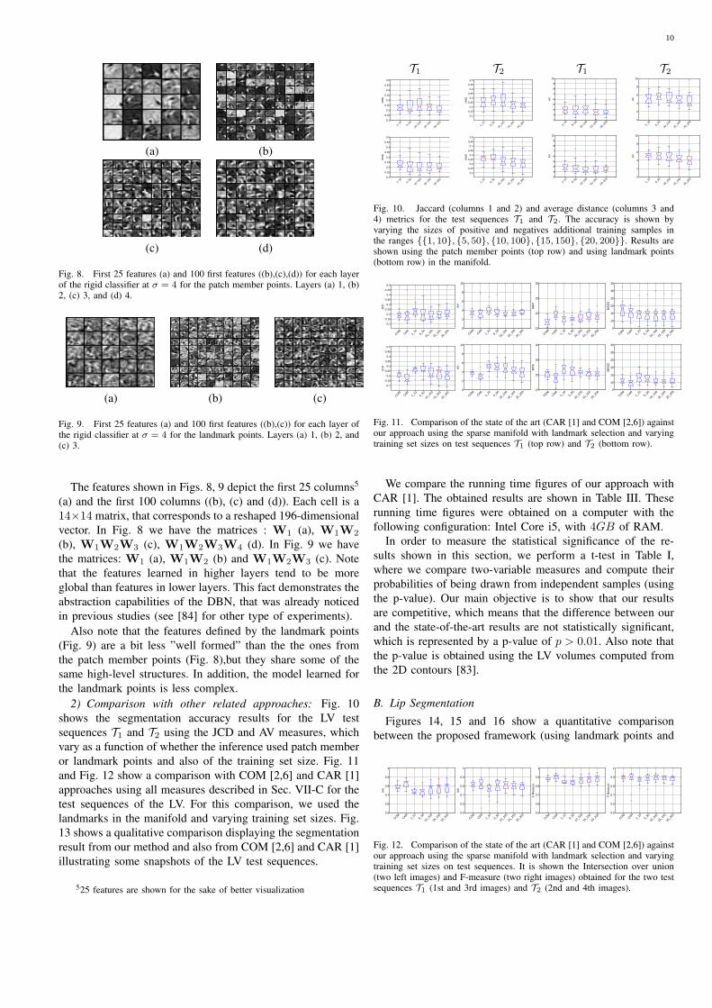
where p(t|x,D) in (2) is represented with p(t|x, γMAP) [52]hereafter. Fig.4(a) displays the training process explained inthis section, where the positive samples are extracted fromthe green region in the center, and the negative samples aredrawn from the yellow region. The parameters λ of the non-rigid classifier in (2) are learned in a similar way with thefollowing optimization:

λMAP = argmaxλ

|P|∏i=1

|Pi|∏j=1

p(yi,j |ti,j ,xi,j , λ), (15)

(a) Training (b) Inference

Fig. 4. The proposed training (a) and inference (b) procedures using sparsemanifolds (please see text for details).

where p(y|t,x,D) in (2) is represented withp(y|t,x, λMAP) [52] hereafter.

The estimation of the segmentation contour follows aninference procedure that takes a test image x as the input,and outputs the contour y∗ ∈ R2S using (1). Recall that, thisinference strategy uses each landmark ti,j (for j ∈ 1, ..., Li)from each learned patch Pi as initial guesses for a gradientascent (GA) procedure [78] on the output of the classifierp(t|x, γMAP) over the search parameter space on the manifoldM. Given that the initial guesses of the GA procedure comefrom the landmarks, we have t

(0)i,j = ti,j , and after N GA iter-

ations, the final value for the search parameter is t(N)i,j , where

the superscript (n) for n ∈ 0, ..., N represents the GA iter-ation index. Assuming that p(t) = p(t|x, γMAP ), the GA al-

gorithm uses the Jacobian ∇p(t) =[

∂p(t)∂t(1) ... ∂p(t)

∂t(M)

]⊤,

which is computed numerically using central difference, withstep size mi (13), as follows:

∂p(t)

∂t(1)=

p(t+ [mi(1)/2, ..., 0]⊤)− p(t− [mi(1)/2, ..., 0]

⊤)

mi(1)(16)

where the parameter for t(.) stands for the dimensionalityindex and t(1) denotes the first dimension of t, and similarlyfor mi(.). In (16), the parameter t ± [mi(1)/2, ..., 0]

⊤ isprojected to the patch Pi (i.e., y = ξi(t)) in order to guaranteethat it belongs to the manifold M. Once the GA process isover and the parameter t(N)

i,j is reached for each landmark ti,jof each patch Pi, the contour y∗ is estimated with a Monte-Carlo approximation of (1) as follows:

y∗ =1

Z

|P|∑i=1

Li∑j=1

y × p(t(N)i,j |x, γMAP)× p(y|t(N)

i,j ,x, λMAP),

(17)where Z is a normalization constant. Figure 4(b) shows thesetting of the segmentation procedure, with the level setsrepresenting the results of the rigid classifier p(ti,j |x, γMAP).Notice that the rigid search procedure is performed only in thelow dimensional space of t.

VI. SEARCH COMPLEXITY REDUCTION

One of the bottlenecks of current top-down non-rigid seg-mentation methods lies in the number of executions of therigid classifier p(t|x, γMAP) that runs in the intermediatespace represented by the variable t ∈ Rr, where r = R

7

indicates the original rigid search space and r = M denotesthe reduced dimensionality search space. For the complexityanalysis below, assume that K = O(103) denotes the numberof samples used in each dimension of this intermediate space.An exhaustive search in this r-dimensional space representsa running time complexity of O(Kr), which is in generalintractable for relatively small values of r = R (note thatR ∈ 4, 5 in state-of-the-art approaches). The reduction ofthis running time complexity has been studied by Lampert etal. [79], who proposed a branch-and-bound approach that canfind a global optimum in this rigid search space in O(Kr/2).Zheng et al. [5] proposed the marginal space learning thatfinds local optima using a coarse-to-fine approach, where thesearch space is recursively broken into spaces of increasingdimensionality (i.e., the search begins with one of the rdimensions, whose result is used to constrain the search inthe space of two dimensions, until arriving at the space of rdimensions). Carneiro et al. [1] also proposed a local optimaapproach based on a coarse-to-fine derivative-based search thatuses a gradient ascent approach in the space of r dimensions.In general, these last two methods provide a search complexityof O(K+ ♯ σ×Kfine× r), where ♯ σ is the number of scales(for the methods above, ♯ σ = 3), with σ ∈ 4, 8, 16, andKfine << K (commonly, Kfine = O(101)).

In the proposed approach, we are able to reduce thecomplexity of the rigid segmentation, that is, reduce r fromR to M , and in this way, increase the efficiency of thissegmentation stage. Therefore, in methods that only haveone coarse step [1,80], represented by the rigid detector, thissmaller dimensionality allows for a faster search process;and for methods that rely on multiple coarse steps [5], ourapproach can reduce the number of coarse steps to run (e.g.,from R to M steps). Thus, if we are using the patch memberpoints (without manifold sparsity) the complexity is given byO((

∑i Pi)×♯ σ×r), meaning that we have to perform the seg-

mentation in every patch of the manifold. When using sparsity,we use of Li landmarks per patch Pi, we avoid the expensiveinitial search of K points in the coarsest scale. Taking all thistogether, we have a final complexity of O((

∑i Li)× ♯ σ× r).

Typically, we have∑

i Li = O(101), so our approach leads toa complexity of O(3× 10× r), which compares favorably toO(103+3×10×r) [1,5] and O((103)r/2) [79]. One possibledrawback of our proposal resides in the frequent use of theparametrization to map t to annotation y, but we show in theexperiments that the cost associated with that procedure is notsignificant compared to the running time of the rigid classifier.

VII. EXPERIMENTAL SETUP

This section presents the experimental setup used for testingthe proposed framework for object segmentation. Recall thatthe objectives of the proposed methodology are: 1) achievesuperior efficiency with competitive accuracy, when comparedto the state of the art, and 2) reach high robustness to smalltraining sets given that training samples are constrained to liein the learned low-dimensional manifold. It is important toemphasize that the inference efficiency depends not only onthe dimensionality of the manifold (that is the tangent space),

but also on the number of landmarks. Therefore, in order totest the robustness of the inference process to a limited numberof landmark points, we run two experiments. In one of theexperiments, we only use the landmarks during the inferenceprocess, making the whole process quite efficient. In the otherexperiment, we use all patch member points, which decreasesignificantly the search efficiency, but can potentially improvethe segmentation accuracy. In order to assess the robustness ofthe learning process to training sets of different sizes, we trainthe rigid detector using augmented training sets of differentsizes. The segmentation results of our methodology are thencompared related approaches in terms of accuracy and runningtime figures.

A. Material

Two different problems are considered in order to em-pirically demonstrate our claims. The first problem is thesegmentation of the left ventricle (LV) of the heart fromultrasound sequences [28], and the second problem is thesegmentation of lips from sequences containing the faces ofseveral people showing different types of emotions [8].

For the LV segmentation problem, 14 sequences taken from14 different subjects are considered, where 12 sequencespresent some kind of cardiopathy (e.g., mild to severe dilationof the LV, hypertrophy of the LV, wall motion abnormalities,dysfunction of the LV, and valvular heart disease) and are usedfor training; 2 sequences are normal and used for testing (i.e.,there is no overlap between subjects in training and test sets).All these sequences display the left ventricle of the heart usingthe apical two and four-chamber views (note that we refer tothe test sets as T1 and T2). We worked with a cardiologist,who annotated 400 images in the training set (an average of 34images per sequence) and 80 images in (average of 40 imagesper sequence) in the test set. It is important to mention thatthe annotations in the training set contain the same numberof keypoints, and that the base and apical points are explicitlyidentified in order for us to determine the rigid transformationbetween each annotation and the canonical location of suchpoints in the reference patch.

For the lip segmentation problem, we use the Cohn-Kanade(CK+) database [8] of emotion sequences taken from frontalview, where the manual lip annotation is available. Amongseveral emotion sequences we take the “happy” and “surprise”sequences, since they contain more challenging lip bound-ary deformations in comparison with the remaining emotionsequences. The training sets contain 12 sequences with 7subjects where we use 5 “happy” sequences and 5 “surprise”sequences, with 3 subjects being used in both sequences, butexhibiting different lip motions. This training set consists of209 frames for training , with 91 and 118 frames of the“happy” and “surprise” sequences, respectively. The test setalso contains 12 sequences with 24 subjects where none ofthe subjects in the test sequences are present in the trainingsequences. This test set comprises 444 images, with 250frames for “happy” and 194 frames for “surprise”.

8

−100−50

050

100150

−50

0

50

100−60

−40

−20

0

20

40

60

−100

−50

0

50

100

−60

−40

−20

0

20

40

60−30

−20

−10

0

10

20

30

Fig. 5. Manifold learning algorithm for the LV (left) and lip (right)segmentation problems. The graphs show the annotation points in blue andlandmarks in red after a PCA reduction. From our experiments, a total of1158 patch member points (blue dots) and 63 landmark points (circle red) areestimated for the LV case. The right graph (lip case) depicts the manifoldestimation with 395 patch-member points (in blue dots) and with the 46landmarks (in red circles). Notice that larger number of patch member points(and landmarks) are obtained for the LV case, which is due to larger LV shapedeformation obtained across different patients.

B. Methods

The dimensionality of the explicit representation for the LVcontour is S = 21 (i.e., 21 2− dimensional points), and forthe lip contour is S = 40 (i.e., 40 2−dimensional points).For the LV segmentation problem, the manifold learningalgorithm produces: (i) |P| = 14 patches, with a total of1158 patch member points and 63 landmark points, and (ii)M = 2 for the dimensionality of the rigid search space (i.e.,this represents the intrinsic dimensionality of the manifold).For the lip segmentation, the manifold learning produces:(i) |P| = 4 patches with 395 patch-member points and 46landmark points, and (ii) M = 2 for the dimensionality ofthe rigid search space. It is worth mentioning that the originaldimensionality of the rigid search space is R = 5 (representingtwo translation, one rotation and two scale parameters), whichis the dimensionality usually found in current state-of-the-artmethods [1,2,6]. Fig. 5 illustrates the result of our manifoldlearning algorithm on the LV and lip segmentation problems(see Section VIII), where each patch Pi contains a set ofthe patch-member and landmark points. In this figure, theblue dots are the annotations after PCA reduction (the firstthree components are shown), and the red circles indicate theestimated landmarks.

The training and inference methods used in this paperare adapted from a methodology that we have proposedrecently [1], consisting of a coarse-to-fine rigid detectorp(t|x, γMAP) and a non-rigid classifier p(y|t,x, λMAP) basedon deep belief networks (DBN) [77]. The main difference liesin the use of sparse low-dimensional manifolds to representthe rigid detection space, which means that we re-trained thecoarse-to-fine rigid detector to run on the learned manifold.Moreover, our rigid classifier is estimated using training setsof different sizes, where we show that the number of additional(artificial) training samples can be reduced with the use of ourlow-dimensionality manifold. Specifically, we vary the size ofthe set of positive samples by varying the number of additionalpositive and negative samples per training image, as follows|T+(i, j)| ∈ 1, 5, 10, 15, 20, and the size of negative samples

as |T−(i)| ∈ 10, 50, 100, 150, 200, as explained in (12)4. Weadded more additional negative samples due to the larger areaoccupied by the negative region.

The performance of our approach is assessed with a quan-titative comparison over the test sets using the followingstate-of-the-art methods based on machine learning techniquesproposed in the literature for the LV segmentation problem:COM [2,6], CAR [1]. For the lip segmentation, we comparethe performance of our approach only with CAR [1] becausethat was the only one available for comparison in this problem.For both segmentation problems, we also compare the runningtimes between our approach and CAR [1].

C. Accuracy Measurements

The performance is evaluated in terms of contour accuracyusing several metrics commonly adopted in the literature andrunning time spent to perform the object segmentation. Thesegmentation accuracy is assessed using the following errormeasures proposed in the literature: (i) Hausdorff (MAX) [81],(ii) Mean Sum of Squared Distance (MSSD) [6], (iii) Jac-card distance (JCD), (iv) average distance (AV) [28], (v) F-measure, and (vi) the Intersection over Union (IoU), whichare commonly used metrics for contour evaluation.

VIII. EXPERIMENTAL RESULTS

This section presents segmentation results of the proposedapproach for the LV segmentation in ultrasound (US) and inmagnetic resonance imaging (MRI) sequences, and also forthe lip segmentation in video sequences. For the LV in USproblem we conduct two distinct experiments. In Sec. VIII-A.1 we evaluate the accuracy of rigid detection separately, asthis is the focus of the paper. In Sec. VIII-A.2 we comparethe proposed framework with other related approaches tailoredfor the same problem and mentioning the run time figuresobtained, as well as the the quantitative contour assessment.Similarly, for the lip segmentation (see Sec. VIII-B) we alsoperform comparisons concerning both quantitative and runtime figures experiments. Finally, we provide a comparisonbetween the proposed method and the semantic segmentationmodel based on the Convolutional Neural Network (CNN) [82]for the segmentation of the endocardium of the LV in MRI inshort axis (see Section VIII-D).

A. LV Segmentation in US

This section is divided into two parts. First, we evaluatethe accuracy of rigid detection, which is accomplished bypresenting the results of the LV segmentation using an 14-foldcross validation (leave one sequence out). Then, we performa comparison with the state-of-the-art methodologies appliedin the same context (i.e., LV segmentation).

4Note that for both databases, the training of the original algorithm in[1] used |T+| = 10, and |T−| = 100 per image in the training set.

9

1) Comparison between rigid and improvement obtainedwith the non-rigid procedure in the problem of the LV Seg-mentation: To obtain the results of the rigid segmentationswe performed a 14-fold cross validation, where the final resultproduced by the rigid detector is assessed based on the meanshape placed at the center of the detected window. The 14-foldcross validation is accomplished as follows:

(a) Generate 14 versions of the manifold as described inSection IV. Each version of the manifold is obtainedusing 13 sequences for training, leaving one sequence outfor testing. This allows us to obtain the set of landmarkpoints (Section IV-C) for each of the 14 manifolds.

(b) For each manifold, several DBN classifiers are trained, asfollows: for a given configuration of data augmentation(recall from Sec. VII-B that there are five possible config-urations), three classifiers are learned (one for each scaleσ ∈ 4, 8, 16). This amounts a total of 15 classifiers.

(c) The two above steps are repeated 14 times, and producea total of 210 DBN classifiers.

The testing stage comprises the following main steps:

(a) For each frame of each held-out test sequence, 5 seg-mentations are produced (from the five data augmentationversions).

(b) Each sequence is tested in 17 images comprising thesystolic and diastolic phase in the cardiac cycle (notethat these 17 images represent a subset of the annotatedimages per sequence). This means that 14 × 17 = 238segmentations are produced for all 14 sequences for agiven data augmentation configuration.

(c) Considering the five data augmentation possibilities, thisamounts a total of 1190 segmentations.

Figure 6 (top) shows the quantitative performance of theshape produced by the rigid detector (i.e., using Jaccard,average distance and Hausdorff metrics). Figure 6 (bottom)shows the improvement brought by the non-rigid segmentationcompared to the rigid detection. From Fig. 6, we can observethat the non-rigid segmentation always improves the resultfrom the rigid detector, which already produces a reasonablycompetitive result.

We also provide another experiment concerning the scatter-plots of the rigid and non-rigid stages using the 14-foldvalidation for all of the positive-negative configurations. Thisis illustrated in Fig. 7, where each dot represents one of theimages in the left-out sequence. In this experiment we comparethe gold standard LV volume using manual annotations and thecomputer-generated LV volume. To estimate the LV volumefrom 2D contour annotations we use the area-length equation[83] with V = 8A2

3πL , where A denotes the projected surfacearea and L is the distance from upper aortic valve point toapex, V is the resulting volume. In this scatter plot, we see thatthe non-rigid segmentation provides better results comparedwith the rigid segmentation. More specifically, the followingcorrelation coefficients r are obtained: (i) rigid detector: r =0.76, 0.79, 0.78, 0.73, 0.75 (see Fig. 7 top) and (ii) non-rigidsegmentation: r = 0.84, 0.84, 0.89, 0.86, 0.86 (see Fig. 7bottom).

0.1

0.15

0.2

0.25

0.3

0.35

0.4

0.45

0.5

JCD

1−10

5−50

10−1

00

15−1

50

20−2

00

0

5

10

15

20

AV

1−10

5−50

10−1

00

15−1

50

20−2

00

40

50

60

70

MA

X

1−10

5−50

10−1

00

15−1

50

20−2

00

0

0.05

0.1

0.15

0.2

0.25

0.3

0.35

0.4

0.45

JCD

1−10

5−50

10−1

00

15−1

50

20−2

00

Non−Rigid Rigid

0

2

4

6

8

10

12

14

16

18

20

AV

1−10

5−50

10−1

00

15−1

50

20−2

00

Non−Rigid Rigid

0

10

20

30

40

50

60

70

80

MA

X

1−10

5−50

10−1

00

15−1

50

20−2

00

Non−Rigid Rigid

Fig. 6. The performance of the rigid detector in the 14-fold cross validationon the LV data is shown on the top graphs, while the bottom shows theimprovements produced by the non-rigid detector, compared to the initialsegmentation by the rigid detector, represented by the mean shape placedat the center of the detection window. From left to right, the graphs showthe Jaccard, average and Hausdorff measures. Furthermore, all measures areshown with respect to varying sizes of positive and negative additional trainingsamples in the ranges (1, 10), (5, 50), (10, 100), (15, 150), (20, 200).

0 0.5 1 1.5 2 2.5

x 106

0

0.5

1

1.5

2

2.5x 10

6

n = 52r = 0.76y = 0.9x + 4.5e+004p value= 4.2e−011

s0

sgold

0.5 1 1.5 2 2.5 3

x 106

0

0.5

1

1.5

2

2.5x 10

6

n = 52r = 0.79y = 0.78x + −9.7e+003p value= 5.2e−012

s0

sgold

0.5 1 1.5 2 2.5

x 106

0

0.5

1

1.5

2

2.5x 10

6

n = 52r = 0.78y = 0.94x + −1.1e+005p value= 7.9e−012

s0

sgold

0.5 1 1.5 2 2.5

x 106

0

0.5

1

1.5

2

2.5x 10

6

n = 52r = 0.73y = 0.87x + −5.8e+004p value= 1.1e−009

s0

sgold

0.5 1 1.5 2 2.5

x 106

0

0.5

1

1.5

2

2.5x 10

6

n = 52r = 0.75y = 0.93x + −1.3e+005p value= 2.2e−010

s0

sgold

0 0.5 1 1.5 2

x 106

0

0.5

1

1.5

2

2.5x 10

6

n = 52r = 0.84y = 1.2x + 4.3e+004p value= 6.2e−015

s0

sgold

0 0.5 1 1.5 2 2.5

x 106

0

0.5

1

1.5

2

2.5x 10

6

n = 52r = 0.84y = 0.97x + 5.8e+004p value= 7e−015

s0

sgold

0 0.5 1 1.5 2

x 106

0

0.5

1

1.5

2

2.5x 10

6

n = 52r = 0.89y = 1.2x + −1e+005p value= 2.8e−018

s0

sgold

0 0.5 1 1.5 2

x 106

0

0.5

1

1.5

2

2.5x 10

6

n = 52r = 0.86y = 1.2x + −9.6e+004p value= 2.7e−016

s0

sgold

0 0.5 1 1.5 2

x 106

0

0.5

1

1.5

2

2.5x 10

6

n = 52r = 0.86y = 1.2x + −1.2e+005p value= 4e−016

s0

sgold

Fig. 7. Scatter plots with linear regression (top) and Bland-Altman bias plots (bottom). Rigid detection (top) non-rigidsegmentation (bottom) for five data augmentation configurations1, 10, 5, 50, 10, 100, 15, 150, 20, 200.

We also show the type of learned features for the rigiddetector in the deep belief network. Figures 8 and 9 showthe features learned for the configuration of 20-200 (i.e.positive-negative) for the patch member and landmark points,respectively. Denoting Wi with i = 1, ..., nL (nL the numberof layers), as the matrices of weights of the DBN learned forσ = 4, where the number of nodes of the learned architecturesare the following:

• Patch member points: (196× 100), (100× 100), (100×200), (200 × 200), nodes, for layers 1, 2, 3 and 4,respectively;

• Landmark points: (196×100), (100×100), (100×200),nodes, for layers 1, 2 and 3, respectively.

Hence, we have for the patch member points, W1 ∈R196×100, W2 ∈ R100×100, W3 ∈ R100×200, and W4 ∈R200×200. For the landmark points the complexity of thearchitecture is lower providing the following weights matrices,W1 ∈ R196×100, W2 ∈ R100×100, and W3 ∈ R100×200.

10

(a) (b)

(c) (d)

Fig. 8. First 25 features (a) and 100 first features ((b),(c),(d)) for each layerof the rigid classifier at σ = 4 for the patch member points. Layers (a) 1, (b)2, (c) 3, and (d) 4.

(a) (b) (c)

Fig. 9. First 25 features (a) and 100 first features ((b),(c)) for each layer ofthe rigid classifier at σ = 4 for the landmark points. Layers (a) 1, (b) 2, and(c) 3.

The features shown in Figs. 8, 9 depict the first 25 columns5

(a) and the first 100 columns ((b), (c) and (d)). Each cell is a14×14 matrix, that corresponds to a reshaped 196-dimensionalvector. In Fig. 8 we have the matrices : W1 (a), W1W2

(b), W1W2W3 (c), W1W2W3W4 (d). In Fig. 9 we havethe matrices: W1 (a), W1W2 (b) and W1W2W3 (c). Notethat the features learned in higher layers tend to be moreglobal than features in lower layers. This fact demonstrates theabstraction capabilities of the DBN, that was already noticedin previous studies (see [84] for other type of experiments).

Also note that the features defined by the landmark points(Fig. 9) are a bit less ”well formed” than the the ones fromthe patch member points (Fig. 8),but they share some of thesame high-level structures. In addition, the model learned forthe landmark points is less complex.

2) Comparison with other related approaches: Fig. 10shows the segmentation accuracy results for the LV testsequences T1 and T2 using the JCD and AV measures, whichvary as a function of whether the inference used patch memberor landmark points and also of the training set size. Fig. 11and Fig. 12 show a comparison with COM [2,6] and CAR [1]approaches using all measures described in Sec. VII-C for thetest sequences of the LV. For this comparison, we used thelandmarks in the manifold and varying training set sizes. Fig.13 shows a qualitative comparison displaying the segmentationresult from our method and also from COM [2,6] and CAR [1]illustrating some snapshots of the LV test sequences.

525 features are shown for the sake of better visualization

T1 T2 T1 T2

0.1

0.15

0.2

0.25

0.3

0.35

0.4

0.45

0.5

HM

D

1−10

5−50

10−1

00

15−1

50

20−2

00

0.1

0.15

0.2

0.25

0.3

0.35

0.4

0.45

0.5

HM

D

1_10

5_50

10_1

00

15_1

50

20_2

002

3

4

5

6

7

8

9

10

AV

1−10

5−50

10−1

00

15−1

50

20−2

000

2

4

6

8

10

AV

1_10

5_50

10_1

00

15_1

50

20_2

00

0.1

0.15

0.2

0.25

0.3

0.35

0.4

0.45

0.5

HM

D

1−10

5−50

10−1

00

15−1

50

20−2

00

0.1

0.15

0.2

0.25

0.3

0.35

0.4

0.45

0.5

HM

D

1_10

5_50

10_1

00

15_1

50

20_2

002

3

4

5

6

7

8

9

10

AV

1−10

5−50

10−1

00

15−1

50

20−2

000

2

4

6

8

10

AV

1_10

5_50

10_1

00

15_1

50

20_2

00

Fig. 10. Jaccard (columns 1 and 2) and average distance (columns 3 and4) metrics for the test sequences T1 and T2. The accuracy is shown byvarying the sizes of positive and negatives additional training samples inthe ranges 1, 10, 5, 50, 10, 100, 15, 150, 20, 200. Results areshown using the patch member points (top row) and using landmark points(bottom row) in the manifold.

0.1

0.15

0.2

0.25

0.3

0.35

0.4

0.45

0.5

JCD

COMCAR

1_10

5_50

10_1

00

15_1

50

20_2

000

2

4

6

8

10

AV

COMCAR

1_10

5_50

10_1

00

15_1

50

20_2

0015

20

25

30

MA

X

COMCAR

1_10

5_50

10_1

00

15_1

50

20_2

005

10

15

20

25

30

35

MS

SD

COMCAR

1_10

5_50

10_1

00

15_1

50

20_2

00

0.1

0.15

0.2

0.25

0.3

0.35

0.4

0.45

0.5

JCD

COMCAR

1_10

5_50

10_1

00

15_1

50

20_2

000

2

4

6

8

10

AV

COMCAR

1_10

5_50

10_1

00

15_1

50

20_2

0015

20

25

30

MA

X

COMCAR

1_10

5_50

10_1

00

15_1

50

20_2

005

10

15

20

25

30

35

MS

SD

COMCAR

1_10

5_50

10_1

00

15_1

50

20_2

00

Fig. 11. Comparison of the state of the art (CAR [1] and COM [2,6]) againstour approach using the sparse manifold with landmark selection and varyingtraining set sizes on test sequences T1 (top row) and T2 (bottom row).

We compare the running time figures of our approach withCAR [1]. The obtained results are shown in Table III. Theserunning time figures were obtained on a computer with thefollowing configuration: Intel Core i5, with 4GB of RAM.

In order to measure the statistical significance of the re-sults shown in this section, we perform a t-test in Table I,where we compare two-variable measures and compute theirprobabilities of being drawn from independent samples (usingthe p-value). Our main objective is to show that our resultsare competitive, which means that the difference between ourand the state-of-the-art results are not statistically significant,which is represented by a p-value of p > 0.01. Also note thatthe p-value is obtained using the LV volumes computed fromthe 2D contours [83].

B. Lip Segmentation

Figures 14, 15 and 16 show a quantitative comparisonbetween the proposed framework (using landmark points and

0.5

0.6

0.7

0.8

0.9

1

IoU

COMCAR

1_10

5_50

10_1

00

15_1

50

20_2

000.5

0.6

0.7

0.8

0.9

1

IoU

COMCAR

1_10

5_50

10_1

00

15_1

50

20_2

000.5

0.6

0.7

0.8

0.9

1

F M

easu

re

COMCAR

1_10

5_50

10_1

00

15_1

50

20_2

000.5

0.6

0.7

0.8

0.9

1

F M

easu

re

COMCAR

1_10

5_50

10_1

00

15_1

50

20_2

00

Fig. 12. Comparison of the state of the art (CAR [1] and COM [2,6]) againstour approach using the sparse manifold with landmark selection and varyingtraining set sizes on test sequences. It is shown the Intersection over union(two left images) and F-measure (two right images) obtained for the two testsequences T1 (1st and 3rd images) and T2 (2nd and 4th images).

11

Fig. 17. Test lip sequences displaying the “happy” expression. The ground truth (in green) is superimposed with the segmentation results (in red).

Fig. 18. Test lip sequences displaying the “surprise” expression. The ground truth (in green) is superimposed with the segmentation results (in red).

Fig. 13. Qualitative comparison between the expert annotation (GT in blue)and the results of our approach (green), COM (yellow), and CAR (purple).The results show the segmentations for the teste sequence T1 (top row) andfor T2 (bottom row).

TABLE IT-TEST BETWEEN THE VOLUMES ESTIMATED WITH THE PROPOSED

APPROACH AND WITH THE CAR [1] AND COM [2,6] APPROACHES ON

THE LV TEST SEQUENCES.

Training set sizes (positive-negative)1-10 5-50 10-100 15-150 20-200

COM [2,6] p-value 0.316 0.079 0.139 0.249 0.138CAR [1] p-value 0.153 0.028 0.066 0.135 0.067

different training set sizes, using the surprise and happysequences, respectively) and the CAR [1] approach.

We also compare the running times of our approach withCAR [1]. See the obtained results for the happy and surprise

0.1

0.15

0.2

0.25

0.3

0.35

0.4

0.45

0.5

JCD

CAR1_

105_

50

10_1

00

15_1

50

20_2

000

2

4

6

8

10

AV

CAR1_

105_

50

10_1

00

15_1

50

20_2

00

5

10

15

20

MA

X

CAR1_

105_

50

10_1

00

15_1

50

20_2

000

50

100

150

200

250

MA

D

CAR1_

105_

50

10_1

00

15_1

50

20_2

00

2

4

6

8

10

12

14

16

MS

SD

CAR1_

105_

50

10_1

00

15_1

50

20_2

00

0.1

0.15

0.2

0.25

0.3

0.35

0.4

0.45

0.5

JCD

CAR1_

105_

50

10_1

00

15_1

50

20_2

000

2

4

6

8

10

AV

CAR1_

105_

50

10_1

00

15_1

50

20_2

00

5

10

15

20

MA

X

CAR1_

105_

50

10_1

00

15_1

50

20_2

000

50

100

150

200

250

MA

D

CAR1_

105_

50

10_1

00

15_1

50

20_2

00

2

4

6

8

10

12

14

16

MS

SD

CAR1_

105_

50

10_1

00

15_1

50

20_2

00

Fig. 14. Comparison with (CAR) method for the surprise sequences. Errormetrics (from left to right: HMD, AV, MAX, MAD and MSSD) for the surprisesequences. The accuracy is shown varying the sizes of positive and negativesexamples in the range 1, 10, 5, 50, 10, 100, 15, 150, 20, 200.Results are shown using the patch member points (top row) and usinglandmark points (bottom row) in the manifold.

sequences in Table III.6

Figs. 17, 18 show examples of the final lip segmentationproduced by our methodology on the happy and surprise testsequences, along with the manual annotation.

Finally, as in the previous LV sequences, we also performa statistical significance of the results on both test sequences.Table II shows the comparison of the two-variable measuresand the computation of their probabilities of being drawnfrom independent samples (using the p-value). The p-valueis obtained using the lip area computed from the 2D contours.

6Notice that we compute the overall mean of the 12 happy sequencesand 12 surprise sequences.

12

0.1

0.15

0.2

0.25

0.3

0.35

0.4

0.45

0.5JC

D

CAR1_

105_

50

10_1

00

15_1

50

20_2

000

2

4

6

8

10

AV

CAR1_

105_

50

10_1

00

15_1

50

20_2

00

5

10

15

20

25

30

35

40

MA

X

CAR1_

105_

50

10_1

00

15_1

50

20_2

00

50

100

150

200

MA

D

CAR1_

105_

50

10_1

00

15_1

50

20_2

00

5

10

15

20

MS

SD

CAR1_

105_

50

10_1

00

15_1

50

20_2

00

0.1

0.15

0.2

0.25

0.3

0.35

0.4

0.45

0.5

JCD

CAR1_

105_

50

10_1

00

15_1

50

20_2

000

2

4

6

8

10

AV

CAR1_

105_

50

10_1

00

15_1

50

20_2

00

5

10

15

20

25

30

35

40

MA

X

CAR1_

105_

50

10_1

00

15_1

50

20_2

00

50

100

150

200

MA

D

CAR1_

105_

50

10_1

00

15_1

50

20_2

00

5

10

15

20

MS

SD

CAR1_

105_

50

10_1

00

15_1

50

20_2

00

Fig. 15. Comparison with (CAR) method for the happy sequences. Errormetrics (from left to right: HMD, AV, MAX, MAD and MSSD) for the surprisesequences. The accuracy is shown varying the sizes of positive and negativesexamples in the range 1, 10, 5, 50, 10, 100, 15, 150, 20, 200.Results are shown using the patch member points (top row) and usinglandmark points (bottom row) in the manifold.

0.4

0.5

0.6

0.7

0.8

0.9

IoU

CAR1_

105_

50

10_1

00

15_1

50

20_2

000

0.2

0.4

0.6

0.8

IoU

CAR1_

105_

50

10_1

00

15_1

50

20_2

00

0.6

0.65

0.7

0.75

0.8

0.85

0.9

0.95

F M

easu

re

CAR1_

105_

50

10_1

00

15_1

50

20_2

00

0

0.2

0.4

0.6

0.8

1

F M

easu

re

CAR1_

105_

50

10_1

00

15_1

50

20_2

00

Fig. 16. Comparison with (CAR) method for the surprise sequences (1stand 3rd images) and for happy sequences (2nd and 4th images) for IoU (twoleft images) and F measure (two right images). Results are shown using thelandmark points in the manifold.

C. Comparison with Other Classification Methodologies

In this section we perform a comparison between the pro-posed approach and other shallow classification methods, suchas SVM and Random Forests (RF). The SVM and RandomForest (we use 100 decision trees) training is based on theconfiguration of 20, 200 positives and negatives to generatethe input patches. This stage allows the estimation of softconfidences for the two-class (binary) classification task, i.e.object segmentation. For the testing phase, we have to plug inthe two methods in the framework. This is done as describedabove, i.e. given the learned manifold, the landmarks are usedas the initial guesses for the gradient ascent procedure. Theonly difference is that, we replace the learned DBN classifiers,

TABLE IIT-TEST BETWEEN THE AREAS ESTIMATED WITH THE PROPOSED

APPROACH AND WITH THE CAR [1] ON THE SURPRISE AND HAPPY

SEQUENCES.

Training set sizes (positive-negative)1-10 5-50 10-100 15-150 20-200

surprise p-value 0.140 0.085 0.163 0.067 0.271happy p-value 0.047 0.063 0.039 0.030 0.060

TABLE IIIRUNNING TIME FIGURES FOR THE LV AND LIPS EXPERIMENTS. THE

RESULTS ARE SHOWN IN SEC. PER FRAME. IN THE RIGID DETECTION

STAGE THE TIME SPENT FOR THE PARAMETERIZATION IS SHOWN IN

PARENTHESIS.

CAR ProposedTotal Rigid Non-Rigid Total

LV (T1, T2) 7.4 2.20 (1.26) 0.17 2.37

Lips Happy 7.4 2.41 (1.29) 0.19 2.60Surprise 7.4 2.44 (1.30) 0.19 2.63

by the confidences of the two methods in the segmentationprocedure.

0.1

0.15

0.2

0.25

0.3

0.35

0.4

0.45

0.5

JCD

1_10

5_50

10_1

00

15_1

50

20_2

00SVM RF

0

2

4

6

8

10

AV

1_10

5_50

10_1

00

15_1

50

20_2

00SVM RF

0.1

0.15

0.2

0.25

0.3

0.35

0.4

0.45

0.5

JCD

1_10

5_50

10_1

00

15_1

50

20_2

00SVM RF

0

2

4

6

8

10

AV

1_10

5_50

10_1

00

15_1

50

20_2

00SVM RF

Fig. 19. Performance of the SVM and RF for the happy (two left images)and surprise (two right images) sequences. Jaccard distance (JCD) and averagedistance (AV) are used in this study.

In this experiment, we use the surprise and happy sequencesfor comparison purposes. Fig. 19 shows the performance ofthe proposed method for all configurations of the positive andnegative examples, and the performance of the SVM and RF.It is clear that the performance of the shallow methods areless accurate that the proposed methodology. This is somehowexpected since it is well known that RF does not train well onsmall datasets (similar performance is obtained for SVM). Onthe other hand, the better accuracy presented by DBN workswell with small training sets.

We also performed an additional study, that explains thegradient ascent procedure during segmentation. Fig. 20 showsthe evolution of the gradient magnitude of the SVM (left)and the DBN (right) in the 12 surprise sequences. In thisexperiment we use five iterations and we plot the evolutionof the gradient agnitude in one patch of the manifold usingthe configuration 20, 200 for positives and negatives, whereeach line corresponds to the gradient magnitude evolution foreach frame in the sequence. We see that, for the SVM thegradient magnitude is more unstable, which can limit the ac-curacy of the segmentation. For the DBN, we can observe thatthis procedure is more stable, where the classifier results areable to provide a better guidance during the segmentation task.This happens since the classifier has an additional informationabout the features learned in the hidden layers and thus, theycan provide more reliable confidence concerning the objectposition.

1 1.5 2 2.5 3 3.5 4 4.5 50

0.01

0.02

0.03

0.04

0.05

0.06

0.07

0.08

Iterations

Gra

dien

t

1 1.5 2 2.5 3 3.5 4 4.5 50

0.01

0.02

0.03

0.04

0.05

0.06

0.07

0.08

Iterations

Gra

dien

t

Fig. 20. Evolution of the gradient in the segmentation process (a) SVM and(b) DBN.

D. LV Segmentation in MRI

This section provides a comparison of the proposed method-ology with the recently proposed semantic segmentation modelbased on Convolutional Neural Networks (CNNs) [82]. Forthis comparison, we use the publicly available dataset [85]containing 33 sequences acquired from 33 subjects (bothhealthy and diseased), where each sequence comprises 20

13

volumes, covering one cardiac cycle. As in the LV US andlip datasets, the object undergoes a rigid plus non-rigid defor-mation throughout time. In this dataset, the number of slicesin each volume ranged from 5 to 10, with a spacing of 6 - 13mm, where each slice is a 256× 256 image, with a resolutionin the range of [0.93− 1.64] mm per pixel. The ground truthof the LV segmentation in each slice is also provided.

The CNN architecture of the semantic segmentation modelhas 14 layers defined as follows (the size of the input channelsare represented in parenthesis):

• Layer 1: 50 input filters of size 5 × 5, with stride=1, in the’conv’ layer (97× 97)

• Layer 2: activation with ’ReLU’, (97× 97)• Layer 3: max-pooling with size of 2×2, and stride=2, (48×48)• Layer 4: 50-250 input/output filters of size 5× 5 in the ’conv’

layer, (44× 44)• Layer 5: activation with ’ReLU’, (44× 44)• Layer 6: max-pooling with size of 2×2 and stride=2, (22×22)• Layer 7: 250-500 input/output filters of size 5×5 in the ’conv’

layer, (18× 18)• Layer 8: activation with ’ReLU’, (18× 18)• Layer 9: 500-500 input/output filters of size 5×5 in the ’conv’

layer, (14× 14)• Layer 10: activation with ’ReLU’, (14× 14)• Layer 11: 500-500 input/output filters of size 5×5 in the ’conv’

layer, (10× 10)• Layer 12: activation with ’ReLU’, (10× 10)• Layer 13: 2-500 input/output filters of size 10 × 10 in the

’deconv’ layer, (28× 28)• Layer 14: ’loss’, (28× 28)

The hyper paremeters of the network are as follows: (i)batchSize = 10, (ii) numEpochs = 100, (iii) learningRate =0.0001, (iv) weightDecay = 0.0005, (v) momentum = 0.9, and(vi) random Gaussian initialisation with weightInit = 1/100.

Fig. 21. MRI slices during a cardiac cycle (top) and the corresponding CNNoutput (bottom).

The evaluation process of the CNN semantic segmentationmodel and the proposed framework is the same as describedin Sec. VIII-A, that is, performing a leave one sequenceout (i.e. 33-fold cross validation). Fig. 21 shows the originalMRI images of the LV (top) and the semantic segmentationproduced by the CNN (bottom).

For comparison purposes, we compute the mean of IoUvalue per volume for the semantic segmentation and theproposed model. Fig. 22 shows the volumetric IoU coefficientobtained with the two methodologies for each of the 33× 20volumes in the dataset. It is possible to see that the proposedmethod is able to achieve comparable results with the CNNsemantic segmentation model. Also note that most of thevolumes are well segmented. The poorer segmentations canbe identified in the regions of the red pixels in the maps. This

figure shows that both methods perform better in the diastolicphase (roughly at frames 1-5 and 11-20) than in the systolicphase (frames 6-10). This is somehow expected where thestructure to be segmented is small (see the rightmost image inFig. 21, where the high probability map seems less defined).

Fig. 23 shows the quantitative comparison comprising usingthe metrics described in Sec. VII-C. The quantitative perfor-mance of the FCN is comparable, it is shown that the proposedmethodology exhibits competitive results.

2 4 6 8 10 12 14 16 18 20

5

10

15

20

25

30

0.5

0.55

0.6

0.65

0.7

0.75

0.8

0.85

0.9

0.95

1

2 4 6 8 10 12 14 16 18 20

5

10

15

20

25

30

0.5

0.55

0.6

0.65

0.7

0.75

0.8

0.85

0.9

0.95

1

(a) (b)

Fig. 22. Discriminated evaluation of the segmentation of each volume inthe dataset for the CNN (a) and the proposed approach (b). Each map is a 33(patients) × 20 (volumes) matrix. The colormap indicates the IoU, in whichgreen correspond to good segmentation and red to poor segmentation.

0.2

0.3

0.4

0.5

0.6

0.7

0.8

0.9A

CC

UR

AC

Y

Jac_

FCN

Jac_

prop

.

IoU_F

CN

IoU_p

rop.

F Mea

s._FCN

F Mea

s._pr

op.

2

4

6

8

10

AC

CU

RA

CY

AV_FCN

AV_pro

p.

MAX_F

CN

MAX_p

rop.

MAD_F

CN

MAD_p

rop.

Fig. 23. Comparison between the FCN and with the proposed method(“.prop” in the legends )using Jaccard distance, IoU, F measure (left) andAV, MAX and MAD metrics (right).

IX. DISCUSSION

In this section, we first discuss the LV segmentation andthen the lip segmentation results. We conclude the section witha presentation of the limitations of our method.

A. LV segmentation

Concerning the LV segmentation results shown in Fig. 10,we see that the inference process achieves similar accuracywith patch member and landmark points. This is relevantbecause it allows an improvement of 2 orders of magnitudein the inference process. Moreover, the number of additionalpositive and negative samples in the training set also showsinsignificant impact on the accuracy of the methodology, asshown in Figures 10 and 11, which demonstrates that ourmethodology is robust to small training sets, allowing a moreefficient training process. The comparison with the state ofthe art in Fig. 11 and Table II shows that our methodologyproduces competitive segmentation results that are comparableto the current state of the art in this database. It is interestingto see that the training process with 1 additional positive and10 additional negatives achieves results that are comparable to

14

COM [2,6] and CAR [1] (notice the large p-value indicatingstatistically insignificant differences in the results). In termsof running time, our method is about 3 times faster thanCAR [1], but notice that the fact that the landmarks initializeindependent search processes could have been exploited toimprove even more this running time.

B. Lip segmentation

For the lip segmentation results shown in Figures 15 and14 we also notice similar accuracy with patch member andlandmark points. Similarly to the LV segmentation, the numberof additional positive and negative samples in the trainingset also shows insignificant impact on the accuracy of themethodology. The comparison with CAR [1] shows that ourproposed approach is mostly comparable (but actually slightlybetter in the sequence ”happy”), as demonstrated by the resultsin Table II. As observed in the LV segmentation results,the training process for the lip segmentation problem alsoproduces competitive results with only 1 additional positiveand 10 additional negatives. Finally, the running time is alsoalso about 3 times faster than CAR [1].

C. Limitations of the Method

One of the main issues of the methodology is with respect tothe number of estimated patches during the manifold learningprocess. In practice, during the segmentation procedure, weobserve that only a small subset of the patches are importantfor the contour estimation in (17). The large number of patchesis important for the robustness of the methodology, but a moreefficient search process could have been designed to avoid thesearch in patches where the DBN produces a segmentationresult with low confidence. Another issue with the method-ology is with respect to the distribution of landmarks withrespect to rigid deformation. In general, the training set mustcontain a good representation of this distribution in order forour approach to work robustly, because the rigid detectionsearch is limited to the initial landmark locations.

X. CONCLUSION

In this paper, we presented a novel methodology for non-rigid object segmentation. The methodology proposed com-bines the deep learning architecture with the use of manifoldlearning. The main contribution and focus of the articleis the dimensionality reduction of the segmentation contourparametrization for the rigid components. A manifold learningbased approach has been proposed and allows to reduce thedimension of the rigid space. Thus, the framework allowsfor a faster running time in both training and segmentationstages. This is because, the training and parameters searchare both reformulated directly in terms of the sparse manifoldparametrization.

Further work will be focused on other directions. Forinstance, we plan to incorporate a dynamical model using themanifold, where the object dynamics is learned directly in thelow dimensional manifold parameter space. This will allow fora reduction of the computational cost in the prediction step.

As explained above we also plan to parallelize the segmen-tation process given that the landmarks represent independentinitial guesses for the search process. In fact, a fully parallelimplementation can make the whole process 10-times moreefficient.

APPENDIX

In this appendix, we briefly review the main steps of themanifold learning algorithm [75], summarized in Sec. IV (see[86] for supplementary information). Briefly, the algorithmtakes the annotations yj|D|j=1 and produces: (i) the intrinsicmanifold dimensionality, (ii) the partitioning of the manifoldinto patches, and (iii) the charts and parameterizations.

1) Intrinsic Manifold Dimensionality: The estimation of theintrinsic dimensionality relies on a selection process over thesignificant eigenvalues of the following covariance matrix foreach yj [87,88]:

Syj =1

|Byj ,ϵ| − 1

∑yk∈Byj ,ϵ

(yk − µByj ,ϵ)(yk − µByj ,ϵ

)⊤,

(18)where Byj ,ϵ represents a set containing the annotations in theneighborhood of yj within ϵ-radius, µByj ,ϵ

denotes the meanof all annotations in the set Byj ,ϵ, and |.| is the set cardinalityoperator. The intrinsic dimension is found by first computingthe eigendecomposition of (18) for all elements of yj|D|j=1.For each neighborhood, the eigenvalue immediately before thegreatest drop in value should correspond to intrinsic dimensionestimated by

Mj ≡ argmaxi

|λi+1 − λi|, (19)

where λi are the sorted eigenvalues of (18). The globalestimate of the intrinsic dimensionality M is the median overthe estimates Mj , with j ∈ 1, ..., |D| [75].

2) Partitioning of the Manifold into Patches: The partion-ing of the manifold M into p patches P1, ...,Pp is based ona clustering method that uses the concept of principal angles(e.g. [89,90]) and point distance as clustering criteria. The q-principal angles between subspaces spanned by the columnsa and b of two matrices A, B are defined as ([89,90]):

cos θk =|akA⊤Bbk|

||Aak|| ||Bbk||(20)

with k ∈ 1, ..., q, where q = dim(A) = dim(B). Assumingthat the matrices A and B are in fact the matrices Vi and Vj

of column eigenvectors found by the eidendecomposition of(18) on elements i and j of yj|D|j=1, the partitioning methodclusters Vi and Vj that have a maximum principal anglesmaller than a threshold (in this work, this threshold is π/2)and the distance between respective yi and yj is also smallerthan a pre-specified threshold. This process produces a set of|P| patches that covers the manifold M.

Given the |P| patches above, the next step of the learningprocess involves the estimation of the hyperplane for eachone of those patches, which form a local coordinate system

15

for each patch. This process involves the computation of thecovariance matrix for each patch Pi, as follows:

SPi =1

|Pi| − 1

∑yk∈Pi

(yk − µPi)(yk − µPi

)⊤, (21)

where µPirepresents the average of the annotations yk ∈ Pi.

Then, the eigendecomposition

SPi = VPiDPiV⊤Pi

(22)

produces the matrix VPi containing an orthonormal basis thatforms the local coordinate system for Pi.

A description of the clustering algorithm, that allows for theparch formation is given in Algorithm 1.

Algorithm 1 Soft clustering for patch formationi← 0while M not covered do

i← i + 1Start new patch Pi

y0 ← random seed chosen among points not attributed to any patchV0 ← tangent subspace basis at y0 found by PCA in By,ϵ

while not all N points visited dod← distances between all unattributed points and all points in Pi

y∗ ← choose unattributed point with minimum DV∗ ← tangent subspace at y∗θ1, . . . , θn ← principal angles between V0 and V∗if maxk=1,...,n θk < τ and mind < ϵ then

append y∗ to Pi

end ifend while

end while

3) Charts and Parameterizations: Given the partition of Minto |P| patches and the local coordinate system VPi of eachpatch Pi, the chart is obtained by projecting the patch pointyi,j according to

ti,j = ζi(yi,j) (23)

where ζi(yi,j) = [V⊤Pi(yi,j − µPi

)]M , where the operator[.]M truncates the input vector at its first M components. Theinverse mappings (i.e., the parameterizations) is given by

yi,j = ξi(ti,j) = VPi

[t(1)i,j , ..., t

(M)i,j , ξi(ti,j)

]⊤+µPi

(24)

where the remaining 2S −M components of ξi are obtainedthrough Gaussian process [75].

REFERENCES

[1] G. Carneiro and J. C. Nascimento, “Multiple dynamic models fortracking the left ventricle of the heart from ultrasound data using particlefilters and deep learning architectures,” in CVPR, 2010, pp. 2815–2822.

[2] B. Georgescu, X. S. Zhou, D. Comaniciu, and A. Gupta, “Databased-guided segmentation of anatomical structures with complex appearance,”in CVPR, 2005.

[3] Y. Zhan, X. S. Zhou, Z. Peng, and A. Krishnan, “Active schedulingof organ detection and segmentation in whole-body medical images,”in Medical Image Computing and Computer-Assisted Intervention–MICCAI 2008. Springer, 2008, pp. 313–321.

[4] S. Zhang, Y. Zhan, M. Dewan, J. Huang, D. N. Metaxas, and X. S.Zhou, “Towards robust and effective shape modeling: Sparse shapecomposition,” Medical image analysis, vol. 16, no. 1, pp. 265–277, 2012.

[5] Y. Zheng, A. Barbu, B. Georgescu, M. Scheuering, and D. Comaniciu,“Four-chamber heart modeling and automatic segmentation for 3-D car-diac CT volumes using marginal space learning and steerable features,”IEEE Trans. Med. Imaging, vol. 27, no. 11, pp. 1668–1681, 2008.

[6] X. S. Zhou, D. Comaniciu, and A. Gupta, “An information fusion frame-work for robust shape tracking,” IEEE Trans. Pattern Anal. MachineIntell., vol. 27, no. 1, pp. 115–129, 2005.

[7] G. Carneiro, J. C. Nascimento, and A. Freitas, “Robust left ventriclesegmentation from ultrasound data using deep neural networks andefficient search methods,” in IEEE Int. Symp. on Biomedical Imaging,from nano to macro (ISBI), 2010, pp. 1085–1088.

[8] P. Lucey, J. Cohn, T. Kanade, J. Saragih, Z. Ambadar, and I. Matthews,“The extended cohn-kanade dataset (ck+): A complete dataset foraction unit and emotion-specified expression,” in Computer Vision andPattern Recognition Workshops (CVPRW), 2010 IEEE Computer SocietyConference on. IEEE, 2010, pp. 94–101.

[9] L. Zhang and E. Geiser, “An effective algorithm for extracting serialendocardial borders from 2-d echocardiograms,” IEEE Trans. Biomed.Eng., vol. BME-31, pp. 441–447, 1984.

[10] M. Sonka, X. Zhang, M. Siebes, M. Bissing, S. Dejong, S. Collins,and C. Mckay, “Segmentation of intravascular ultrasound images: Aknowledge-based approach,” IEEE Trans. Med. Imag., vol. 14, pp. 719–732, 1995.

[11] O. Bernard, B. Touil, A. Gelas, R. Prost, and D. Friboulet, “A rbf-basedmultiphase level set method for segmentation in echocardiography usingthe statistics of the radiofrequency signal,” in ICIP, 2007.

[12] O. Bernard, D. Friboulet, P. Thevenaz, and M. Unser, “Variational b-spline level-set: A linear filtering approach for fast deformable modelevolution,” IEEE Trans. Imag. Proc., vol. 18, no. 6, pp. 1179–1991,2009.

[13] X. Bresson, S. Esedoglu, P. Vandergheynst, J.-P. Thiran, and S. Osher,“Fast global minimization of the active contour/snake model,” Journalof Mathematical Imaging and vision, vol. 28, no. 2, pp. 151–167, 2007.

[14] C. Corsi, G. Saracino, A. Sarti, and C. Lamberti, “Left ventricularvolume estimation for real-time three-dimensional echocardiography,”IEEE Trans. Med. Imag., vol. 21, no. 9, pp. 1202–1208, 2002.

[15] D. Cremers, S. Osher, and S. Soatto, “Kernel density estimation andintrinsic alignment for shape priors in level set segmentation,” Interna-tional Journal of Computer Vision, vol. 69, no. 3, pp. 335–351, 2006.

[16] E. Debreuve, M. Barlaud, G. Aubert, I. Laurette, and J. Darcourt,“Space-time segmentation using level set active contours applied tomyocardial gated SPECT,” IEEE Trans. Med. Imag., vol. 20, no. 7,pp. 643–659, 2001.

[17] M. Kass, A. Witkin, and D. Terzopoulos, “Snakes: Active contourmodels,” International Journal of Computer Vision, vol. 4, no. 1, pp.321–331, 1987.

[18] N. Lin, W. Yu, and J. Duncan, “Combinative multi-scale level setframework for echocardiographic image segmentation,” Medical ImageAnalysis, vol. 7, no. 4, pp. 529–537, 2003.

[19] M. Lynch, O. Ghita, and P. F. Whelan, “Segmentation of the left ventricleof the heart in 3-D+t MRI data using an optimized nonrigid temporalmodel,” IEEE Trans. Med. Imag., vol. 27, no. 2, pp. 195–203, 2008.

[20] R. Malladi, J. Sethian, and B. Vemuri, “Shape modeling with frontpropagation: A level set approach,” IEEE Trans. Pattern Anal. Mach.Intell., vol. 17, pp. 158–175, 1995.

[21] N. Paragios and R. Deriche, “Geodesic active regions and level setmethods for supervised texture segmentation,” International Journal ofComputer Vision, vol. 46, no. 3, pp. 223–247, 2002.

[22] N. Paragios, “A level set approach for shape-driven segmentation andtracking of the left ventricle,” IEEE Trans. Med. Imag., vol. 22, no. 6,pp. 773–776, 2003.

[23] A. Sarti, C. Corsi, E. Mazzini, and C. Lamberti, “Maximum likelihoodsegmentation of ultrasound images with rayleigh distribution,” IEEE T.on Ult., Fer. and F.C.,, vol. 52, no. 6, pp. 947–960, 2005.

[24] T. Chen, J. Babb, P. Kellman, L. Axel, and D. Kim, “Semiautomatedsegmentation of myocardial contours for fast strain analysis in cinedisplacement-encoded MRI,” IEEE Trans. Med. Imag., vol. 27, no. 8,pp. 1084–1094, 2008.

[25] Q. Duan, E. D. Angelini, and A. Laine, “Real time segmentationby active geometric functions,” Comput. Methods Programs Biomed.,vol. 98, no. 3, pp. 223–230, 2010.

[26] G. Jacob, J. A. Noble, C. Behrenbruch, A. D. Kelion, and A. P. Banning,“A shape-space-based approach to tracking myocardial borders andquantifying regional left-ventricular function applied in echocardiogra-phy,” IEEE Trans. Med. Imag., vol. 21, no. 3, pp. 226–238, 2002.

[27] M. Mignotte, J. Meunier, and J. Tardif, “Endocardial boundary e timationand tracking in echocardiographic images using deformable template andmarkov random fields,” Pattern Analysis and Applications, vol. 4, no. 4,pp. 256–271, 2001.

[28] J. C. Nascimento and J. S. Marques, “Robust shape tracking withmultiple models in ultrasound images,” IEEE Trans. Imag. Proc., vol. 17,no. 3, pp. 392–406, 2008.

[29] V. Zagrodsky, V. Walimbe, C. Castro-Pareja, J. X. Qin, J.-M. Song,and R. Shekhar, “Registration-assisted segmentation of real-time 3-D

16

echocardiographic data using deformable models,” IEEE Trans. Med.Imag., vol. 24, no. 9, pp. 1089–1099, 2005.

[30] L. Bertelli, T. Yu, D. Vu, and B. Gokturk, “Kernelized structural svmlearning for supervised object segmentation,” in Computer Vision andPattern Recognition (CVPR), 2011 IEEE Conference on. IEEE, 2011,pp. 2153–2160.

[31] J. G. Bosch, S. C. Mitchell, B. P. F. Lelieveldt, F. Nijland, O. Kamp,M. Sonka, and J. H. C. Reiber, “Automatic segmentation of echocardio-graphic sequences by active appearance motion models,” IEEE Trans.Med. Imag., vol. 21, no. 11, pp. 1374–1383, 2002.

[32] T. Cootes, C. Beeston, G. Edwards, and C. Taylor, “A unified frameworkfor atlas matching using active appearance models,” in InformationProcessing in Medical Imaging, 1999, pp. 322–333.

[33] T. Cootes, C. Taylor, D. Cooper, and J. Graham, “Active shape models -their training and application,” Comput. Vis. Image Understand., vol. 61,no. 1, pp. 38–59, 1995.

[34] G. Carneiro, J. C. Nascimento, and A. Freitas, “Robust left ventriculesegmentation from ultrasound data using deep neural networks andefficient search methods,” in Int. Symp. Biomedical Imaging: from nanoto macro (ISBI), 2010.

[35] G. Carneiro and J. C. Nascimento, “Multiple dynamic models fortracking the left ventricle of the heart from ultrasound data using particlefilters and deep learning architectures,” in Conf. Computer Vision andPattern Rec. (CVPR), 2010.

[36] G. Carneiro, B. Georgescu, S. Good, and D. Comaniciu, “Detectionand measurement of fetal anatomies from ultrasound images using aconstrained probabilistic boosting tree,” IEEE Trans. Med. Imaging,vol. 27, no. 9, pp. 1342–1355, 2008.

[37] B. Georgescu, X. S. Zhou, D. Comaniciu, and A. Gupta, “Database-guided segmentation of anatomical structures with complex appearance,”in Conf. Computer Vision and Pattern Rec. (CVPR), 2005.

[38] M. Maire, S. X. Yu, and P. Perona, “Object detection and segmentationfrom joint embedding of parts and pixels,” in Computer Vision (ICCV),2011 IEEE International Conference on. IEEE, 2011, pp. 2142–2149.

[39] S. Mitchell, B. Lelieveldt, R. van der Geest, H. Bosch, J. Reiber,and M. Sonka, “Multistage hybrid active appearance model matching:Segmentation of left and right ventricles in cardiac MR images,” IEEETrans. Med. Imag., vol. 20, no. 5, pp. 415–423, 2001.

[40] J. Weng, A. Singh, and M. Chiu, “Learning-based ventricle detectionfrom cardiac mr and ct images,” IEEE Trans. Med. Imag., vol. 16, no. 4,pp. 378–391, 1997.

[41] Y. Zheng, A. Barbu, B. Georgescu, M. Scheuering, and D. Comaniciu,“Four-chamber heart modeling and automatic segmentation for 3-D car-diac CT volumes using marginal space learning and steerable features,”IEEE Trans. Med. Imaging, vol. 27, no. 11, pp. 1668–1681, 2008.

[42] P. Arbelaez, B. Hariharan, C. Gu, S. Gupta, L. Bourdev, and J. Malik,“Semantic segmentation using regions and parts,” in Computer Visionand Pattern Recognition (CVPR), 2012 IEEE Conference on. IEEE,2012, pp. 3378–3385.

[43] T. Brox, L. Bourdev, S. Maji, and J. Malik, “Object segmentation byalignment of poselet activations to image contours,” in Computer Visionand Pattern Recognition (CVPR), 2011 IEEE Conference on. IEEE,2011, pp. 2225–2232.

[44] J. Carreira, R. Caseiro, J. Batista, and C. Sminchisescu, “Semanticsegmentation with second-order pooling,” in Computer Vision–ECCV2012. Springer, 2012, pp. 430–443.

[45] J. M. Gonfaus, X. Boix, J. Van de Weijer, A. D. Bagdanov, J. Serrat,and J. Gonzalez, “Harmony potentials for joint classification and seg-mentation,” in Computer Vision and Pattern Recognition (CVPR), 2010IEEE Conference on. IEEE, 2010, pp. 3280–3287.

[46] P. S. L’ubor Ladicky, K. Alahari, C. Russell, and P. H. Torr, “What,where and how many? combining object detectors and crfs,” in Pro-ceedings of the 11th European conference on Computer vision: Part IV,2010, pp. 424–437.

[47] L. Ladicky, C. Russell, P. Kohli, and P. H. Torr, “Graph cut basedinference with co-occurrence statistics,” in Computer Vision–ECCV2010. Springer, 2010, pp. 239–253.

[48] J. Yao, S. Fidler, and R. Urtasun, “Describing the scene as a whole:Joint object detection, scene classification and semantic segmentation,”in Computer Vision and Pattern Recognition (CVPR), 2012 IEEEConference on. IEEE, 2012, pp. 702–709.

[49] B. Taskar, V. Chatalbashev, D. Koller, and C. Guestrin, “Learningstructured prediction models: A large margin approach,” in Proceedingsof the 22nd international conference on Machine learning. ACM, 2005,pp. 896–903.

[50] I. Tsochantaridis, T. Joachims, T. Hofmann, Y. Altun, and Y. Singer,“Large margin methods for structured and interdependent output vari-ables.” Journal of Machine Learning Research, vol. 6, no. 9, 2005.

[51] P. Viola and M. J. Jones, “Robust real-time face detection,” Internationaljournal of computer vision, vol. 57, no. 2, pp. 137–154, 2004.

[52] G. Carneiro, J. C. Nascimento, and A. Freitas, “The segmentation ofthe left ventricle of the heart from ultrasound data using deep learningarchitectures and derivative-based search methods,” Image Processing,IEEE Transactions on, vol. 21, no. 3, pp. 968–982, 2012.

[53] C. H. Lampert, M. B. Blaschko, and T. Hofmann, “Efficient subwindowsearch: A branch and bound framework for object localization,” PatternAnalysis and Machine Intelligence, IEEE Transactions on, vol. 31,no. 12, pp. 2129–2142, 2009.

[54] U. Helmke, K. Huper, P. Y. Lee, and J. Moore, “Essential matrixestimation using Gauss-Newton iterations on a manifold,” Int. Journalof Comp. Vision, vol. 74, no. 2, pp. 117–136, 2007.

[55] K. Huper and J. Trumpf, “Newton-like methods for numerical optimiza-tion on manifolds,” in In Proc. of the 38th Asilomar Conference onSignals, Systems and Computers, vol. 1, 2004, pp. 136–139.

[56] P.-A. Absil, R. Mahony, and R. Sepulchre, “Riemmanian geometry ofGrassman manifolds with a view on algorithmic computation,” in ActaApplicandae Mathematicae, vol. 80, 2004, pp. 199–220.

[57] A. Edelman, T. Arias, and S. Smith, “The geometry of algorithms withorthogonality consraints,” in SIAM J. Matrix Anal. Appl., vol. 20, no. 2,1998, pp. 303–353.

[58] S. Smith, “Optimization techniques on Riemmanian manifolds,” in InHamiltonian and gradient flows, algorithms and control, A. Bloch, Ed.American Mathematical Society, 2004, pp. 113–136.

[59] I. F. Gorodnitsky, J. S. George, and B. D. Rao, “Neuromagnetic sourceimaging with focuss: A recursive weighted minimum norm algorithm,”Electroencephalogr. Clin. Neurophysiol., vol. 95, no. 4, pp. 231–251,1995.

[60] S. F. Cotter, B. D. Rao, K. Engan, and K. Kreutz-Delgado, “Sparsesolutions to linear inverse problems with multiple measurement vectors,”IEEE Trans. Signal Processing, vol. 53, no. 7, pp. 2477–2488, 2005.

[61] B. K. Natarajan, “Sparse approximate solutions to linear systems,” SIAMJ. Comput., vol. 24, no. 2, pp. 227–234, 1995.

[62] E. S. Cheng, S. Chen, and B. Mulgrew, “Efficient computational schemesfor the orthogonal least squares learning algorithm,” IEEE Trans. SignalProcessing, vol. 43, no. 1, pp. 373–376, 1995.

[63] S. Chen and J.Wigger, “Fast orthogonal least squares algorithm forefficient subset model selection,” IEEE Trans. Signal Processing, vol. 43,no. 7, pp. 1713–1715, 1995.

[64] S. F. Cotter, J. Adler, B. D. Rao, and K. Kreutz-Delgado, “Forwardsequential algorithms for best basis selection,” Proc. Inst. Elect. Eng.Vision, Image, Signal Process., vol. 146, no. 5, pp. 235–244, 1999.

[65] S. Chen and D. Donoho, “Basis pursuit,” in Asilomar Conf. Signals,Syst., Comput., vol. I, 1994, pp. 41–44.

[66] S. S. Chen, D. L. Donoho, and M. A. Saunders, “Atomic decompositionby basis pursuit,” SIAM J. Sci. Comput., vol. 21, no. 1, pp. 33–61, 1998.

[67] B. D. Rao, K. Engan, S. F. Cotter, J. Palmer, and K. Kreutz-Delgado,“Subset selection in noise based on diversity measure minimization,”IEEE Trans. Signal Processing, vol. 51, no. 3, pp. 760–770, 2003.

[68] J. A. Tropp, “Algorithms for simultaneous sparse approximation part ii:Convex relaxation,” Signal Process. (Special Issue on Sparse Approxi-mations in Signal and Image Processing), vol. 86, pp. 589–602, 2006.

[69] J. Chen and X. Huo, “Theoretical results on sparse representations ofmultiple-measurement vectors,” IEEE Trans. Signal Processing, vol. 54,no. 12, pp. 4634–4643, 2006.

[70] Y. Eldar and M. Mishali, “Robust recovery of signals from a structuredunion of subspaces,” IEEE Trans. Inform. Theory, vol. 55, no. 11, pp.5302–5316, 2009.

[71] L. Sun, J. Liu, J. Chen, and J. Ye, “Efficient recovery of jointly sparsevectors,” in NIPS, 2009.

[72] J. C. Nascimento, J. G. Silva, J. S. Marques, and J. Lemos, “Manifoldlearning for object tracking with multiple nonlinear models,” IEEETrans. on Imag. Proc., vol. 23, no. 4, pp. 1593–1605, 2014.

[73] J. C. Nascimento and G. Carneiro, “Top-down segmentation of non-rigid visual objects using derivative-based search on sparse manifolds,”in CVPR, 2013, pp. 1963–1970.

[74] T. Poggio and S. Smale, “The mathematics of learning: Dealing withdata,” Notices of the American Mathematical Society, vol. 50, no. 5, pp.537–544, 2003.

[75] J. C. Nascimento and J. G. Silva, “Manifold learning for object trackingwith multiple motion dynamics,” in ECCV, 2010.

[76] B. Efron, T. Hastie, I. Johnstone, and R. Tibshirani, “Least angleregression,” Ann. Statist., vol. 32, no. 2, pp. 407–499, 2004.

17

[77] G. Hinton and R. Salakhutdinov, “Reducing the dimensionality of datawith neural networks,” Science, vol. 313, no. 5786, pp. 504–507, 2006.

[78] S. Boyd and L. Vandenberghe, Convex Optimization. CambridgeUniversity Press, March 2004.

[79] C. H. Lampert, M. B. Blaschko, and T. Hofmann, “Beyond slidingwindows: Object localization by efficient subwindow search,” in CVPR,2008.

[80] S. Zhou, J. Zhou, and D. Comaniciu, “A boosting regression approachto medical anatomy detection,” in Proc. of the IEEE Conf. on Comp.Vision Pattern Recognition, pp. 1–8.

[81] D. Huttenlocher, G. Klanderman, and W. Rucklidge, “Comparing imagesusing hausdorff distance,” IEEE Trans. Pattern Anal. Mach. Intell.,vol. 15, no. 9, pp. 850–863, 1993.

[82] J. Long, E. Shelhamer, and T. Darrell, “Fully convolutional networksfor semantic segmentation,” in CVPR, 2015.

[83] J. C. Reiber, A. R. Viddeleer, G. Koning, M. J. Schalij, and P. E. Lange,“Left ventricular regression equations from single plane cine and digitalX-ray ventriculograms revisited,” Clin. Cardiology, vol. 12, no. 2, pp.69–78, 1996, kluwer Academic Publishers.

[84] R. Salakhutdinov and G. Hinton, “Learning a non-linear embedding bypreserving class neighbourhood structure,” in AI and Statistics, 2007.

[85] A. Andrepoulos and J. K. Tsotos, “Efficient and generalizable statisticalmodels of shape and appearance for analysis of cardiac mri,” Med. ImageAnal., vol. 12, no. 3, pp. 335–357, 2008.

[86] J. G. Silva, J. S. Marques, and J. M. Lemos, “Selecting landmark pointsfor sparse manofold learning,” in NIPS, 2005.

[87] J. Bruske and G. Sommer, “Intrinsic dimensionality estimation with op-timally topology preserving maps,” IEEE Trans. Pattern Anal. MachineIntell., vol. 20, pp. 572–575, 1997.

[88] K. Fukunaga and D. R. Olsen, “An algorithm for finding intrinsicdimensionality of data,” IEEE Trans. on Computers, no. 2, pp. 176–183, 1971.

[89] A. Bjorck and G. H. Golub, “Numerical methods for computing anglesbetween linear subspaces,” no. 123, pp. 579–594, 1973.

[90] P. A. Wedin, “On angles between subspaces of a finite dimensional innerproduct space,” in Matrix Pencils, 1983, pp. 263–285.

Jacinto C. Nascimento (S’00 - M’06) received theE.E. degree from the Instituto Superior de Engen-haria de Lisboa, Lisbon, Portugal, and the M.Sc. andPh.D. degrees in electrical and computer engineeringfrom the Instituto Superior Tecnico(IST), TechnicalUniversity of Lisbon, Lisbon, in 1995, 1998, and2003, respectively. He has been with the Facultyof the Department of Informatics and ComputerEngineering, IST, since 2013, where he is currentlya Assistant Professor. His research interests includestatistical image processing, pattern recognition, ma-

chine learning, deep learning medical imaging analysis, video surveillance,general visual object classification. He has coauthored more than 30 publica-tions in international journals (many of which are sponsored by the IEEE),has served on program committees of many international conferences, andhas been a reviewer for several international journals. He is a member of theIEEE.

Gustavo Carneiro received the BS and MSc degreesin computer science from the Federal Universityof Rio de Janeiro and the Military Institute ofEngineering, Brazil, in 1996 and 1999, respectively,and the PhD degree in computer science from theUniversity of Toronto, Canada, in 2004. Currently,an associate professor in the School of ComputerScience at the University of Adelaide, Australia.Previously, he worked at the Instituto Superior Tec-nicoof Lisbon, from 2008 to 2011 as a visitingresearcher and assistant professor, and from 2006

to 2008, he worked at Siemens Corporate Research in Princeton, NewJersey. His research interests include medical image analysis, image featureselection and extraction, content-based image retrieval and annotation, andgeneral visual object classification. He was the recipient of a Marie CurieInternational Incoming Fellowship and has authored more than 50 peerreviewed publications in international journals and conferences.