Deep Recurrent Neural Networks for Acoustic Modelling

William Chan1, Ian Lane1,2

Carnegie Mellon University1Electrical and Computer Engineering, 2Language Technologies Institute

williamchan@cmu.edu, lane@cmu.edu

AbstractWe present a novel deep Recurrent Neural Network (RNN)model for acoustic modelling in Automatic Speech Recognition(ASR). We term our contribution as a TC-DNN-BLSTM-DNNmodel, the model combines a Deep Neural Network (DNN)with Time Convolution (TC), followed by a Bidirectional Long-Short Term Memory (BLSTM), and a final DNN. The first DNNacts as a feature processor to our model, the BLSTM then gen-erates a context from the sequence acoustic signal, and the finalDNN takes the context and models the posterior probabilities ofthe acoustic states. We achieve a 3.47 WER on the Wall StreetJournal (WSJ) eval92 task or more than 8% relative improve-ment over the baseline DNN modelsIndex Terms: Deep Neural Networks, Recurrent Neural Net-works, Long-Short Term Memory, Asynchronous StochasticGradient Descent, Automatic Speech Recognition

1. IntroductionDeep Neural Networks (DNNs) and Convolutional Neural Net-works (CNNs) have yielded many state-of-the-art results inacoustic modelling for Automatic Speech Recognition (ASR)tasks [1, 2]. DNNs and CNNs often accept some spectral fea-ture (e.g., log-Mel filter banks) with a context window (e.g., +/-10 frames) as inputs and trained via supervised backpropaga-tion with softmax targets learning the Hidden Markov Model(HMM) acoustic states.

DNNs do not make much prior assumptions about the inputfeature space, and consequently the model architecture is blindto temporal and frequency structural localities. CNNs are ableto directly model local structural localities through the usage ofconvolutional filters. CNN filters connect to only a subset re-gion of the feature space and are tied and shared across the en-tire input feature, giving the model translational invariance [3].Additionally, pooling is often added, which yields rotational in-variance [2]. The inherent structure of CNNs yields a modelmuch more robust to small shifts and permutations.

Speech is fundamentally a sequence of time signals. CNNs(with time convolution) can capture some of this time localitythrough the convolution filters, however CNNs may not be ableto directly capture longer temporal signal patterns. For exam-ple, temporal patterns may span 10 or more frames, however theconvolution filter width may only be 5 frames wide. The CNNmodel must then rely on the higher level fully connected layersto model these long term dependencies. Additionally, one sizemay not fit all, the frame width of phones and temporal patternsare of varying lengths. Optimizing the convolution filter size isa expensive procedure and corpora dependent [4].

Recently, Recurrent Neural Networks (RNNs) have beenintroduced demonstrating power modelling capabilities for se-quences [5, 6, 7, 8]. RNNs incorporate feedback cycles in the

network architecture. RNNs include a temporal memory com-ponent (for example, in LSTMs the cell state [9]), which allowsthe model to store temporal contextual information directly inthe model. This relieves us from explicitly defining the sizeof temporal contexts (e.g., the time convolution filter size inCNNs), and allows the model to learn this directly. In fact in[8], the whole speech sequence can be accumulated in the tem-poral context.

There exist many implementations of RNNs [10]. LSTMand Gated Recurrent Units (GRUs) [10] are particular imple-mentations of RNNs that are easy to train and do not suffer fromthe vanishing or exploding gradient problems when perform-ing Backpropagation Through Time (BPTT) [11]. LSTMs havethe capability to remember sequences with long range temporaldependencies [9] and have been applied successfully to manyapplications include image captioning [12], end-to-end speechrecognition [13] and machine translation [14].

LSTMs process sequential signals in one direction. Onenatural extension is bidirectional LSTMs (BLSTMs), which iscomposed of two LSTMs. The forward LSTM process the se-quence as usual (e.g., reads the input sequence in the forwarddirection), the second processes the input sequence in backwardorder. The outputs of the two sequences can then be concate-nated. BLSTMs have two distinct advantages over LSTMs, thefirst advantage being the forward and backward passes of the se-quence yields differing temporal dependencies, the model cancapture both sets of the signal dependencies. The second advan-tage is the higher level sequence layers (e.g., stacked BLSTMs)using the BLSTM outputs can access information from both in-put directions.

LSTMs and GRUs (and their bidirectional variants) have re-cently been successfully applied to acoustic modelling and ASR[5, 7, 8]. In [5] TIMIT phone sequences were trained end-to-end from unsegmented sequence data using a LSTM transducer.LSTMs can be combined with Connectionist Temporal Classifi-cation (CTC) and implicitly perform sequence training over thespeech signal on TIMIT [7]. [15] used GRUs and generated anexplicit alignment model between the TIMIT speech sequencedata to the phone sequence. In [8] a commercial speech sys-tem is trained using a LSTM acoustic model, here the the entirespeech sequence is used as the context for classifying contextdependent phones. [16] extend from [8] and applied sequencetraining on top of LSTMs. Our contribution in this paper isa novel deep RNN acoustic model which is easy to train andarchives an 8% relative improvement over DNNs for the WallStreet Journal (WSJ) corpus.

2. ModelOur model architecture can be summarized as a TC-DNN-BLSTM-DNN acoustic model. Our model deals with fixed

arX

iv:1

504.

0148

2v1

[cs

.LG

] 7

Apr

201

5

fMLLR Features40 dimensional

features with time convolution

2 Layer ReLU DNNProject our acoustic features to a high dimensional space

2 Layer ReLU DNNNon-linear projections of the BLSTM context

BLSTMModel the sequential

signal with a RNN and generate a context

Softmax Classification3431 acoustic states

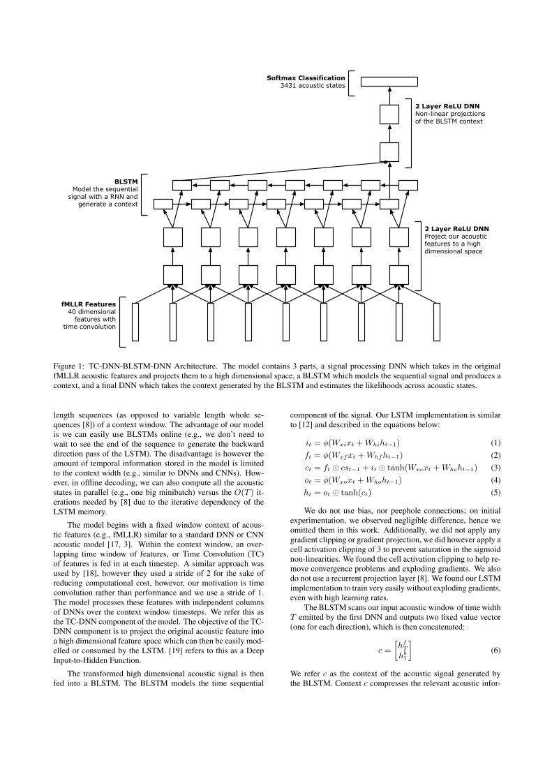
Figure 1: TC-DNN-BLSTM-DNN Architecture. The model contains 3 parts, a signal processing DNN which takes in the originalfMLLR acoustic features and projects them to a high dimensional space, a BLSTM which models the sequential signal and produces acontext, and a final DNN which takes the context generated by the BLSTM and estimates the likelihoods across acoustic states.

length sequences (as opposed to variable length whole se-quences [8]) of a context window. The advantage of our modelis we can easily use BLSTMs online (e.g., we don’t need towait to see the end of the sequence to generate the backwarddirection pass of the LSTM). The disadvantage is however theamount of temporal information stored in the model is limitedto the context width (e.g., similar to DNNs and CNNs). How-ever, in offline decoding, we can also compute all the acousticstates in parallel (e.g., one big minibatch) versus the O(T ) it-erations needed by [8] due to the iterative dependency of theLSTM memory.

The model begins with a fixed window context of acous-tic features (e.g., fMLLR) similar to a standard DNN or CNNacoustic model [17, 3]. Within the context window, an over-lapping time window of features, or Time Convolution (TC)of features is fed in at each timestep. A similar approach wasused by [18], however they used a stride of 2 for the sake ofreducing computational cost, however, our motivation is timeconvolution rather than performance and we use a stride of 1.The model processes these features with independent columnsof DNNs over the context window timesteps. We refer this asthe TC-DNN component of the model. The objective of the TC-DNN component is to project the original acoustic feature intoa high dimensional feature space which can then be easily mod-elled or consumed by the LSTM. [19] refers to this as a DeepInput-to-Hidden Function.

The transformed high dimensional acoustic signal is thenfed into a BLSTM. The BLSTM models the time sequential

component of the signal. Our LSTM implementation is similarto [12] and described in the equations below:

it = φ(Wxixt +Whiht−1) (1)ft = φ(Wxfxt +Whfht−1) (2)ct = ft � cst−1 + it � tanh(Wxcxt +Whcht−1) (3)ot = φ(Wxoxt +Whoht−1) (4)ht = ot � tanh(ct) (5)

We do not use bias, nor peephole connections; on initialexperimentation, we observed negligible difference, hence weomitted them in this work. Additionally, we did not apply anygradient clipping or gradient projection, we did however apply acell activation clipping of 3 to prevent saturation in the sigmoidnon-linearities. We found the cell activation clipping to help re-move convergence problems and exploding gradients. We alsodo not use a recurrent projection layer [8]. We found our LSTMimplementation to train very easily without exploding gradients,even with high learning rates.

The BLSTM scans our input acoustic window of time widthT emitted by the first DNN and outputs two fixed value vector(one for each direction), which is then concatenated:

c =

[hfT

hb1

](6)

We refer c as the context of the acoustic signal generated bythe BLSTM. Context c compresses the relevant acoustic infor-

mation needed to classify the phones from the feature context(e.g., the window of fMLLR features).

The context is further manipulated and projected by a sec-ond DNN. The second DNN adds additional non-linear trans-formations before being finally fed to the softmax layer tomodel the context dependent state posteriors. [19] refers thisas the Deep Hidden-to-Output Function. The model is trainedsupervised with backpropagation minimizing the cross entropyloss. Figure 1 gives a visualization of our entire model.

3. OptimizationWe found our LSTM models to be very easy to train and con-verge. We initialize our LSTM layers with a uniform distri-bution U(−0.01, 0.01), and our DNN layers with a GaussiandistributionN (0, 0.001). We clip our LSTM cell activations to3, we did not need to apply any gradient clipping or gradientprojection.

We train our model with Stochastic Gradient Descent(SGD) using a minibatch size of 128, we found using largerminibatches (e.g., 256) to give slightly worse WERs. We used asimple geometric decay schedule, we start with a learning rateof 0.1 and multiply it by a factor of 0.5 every epoch. We havea learning rate floor of 0.00001 (e.g., the learning rate does notdecay beyond this value). We experimented with both classi-cal and Nesterov momentum, however we found momentum toharm the final WER convergence slightly, hence we use no mo-mentum. We apply the same optimization hyperparameters forall our experiments, it is possible using a slightly different de-cay schedule will yield better results. Our best model took 17epochs to converge or around 51 hours in wall clock time witha NVIDIA Tesla K20 GPU.

4. Experiments and ResultsWe experiment with the WSJ dataset. We use si284 with ap-proximately 81 hours of speech as the training set, dev93 as ourdevelopment set and eval92 as our test set. We observe the WERof our development set after every epoch, we stop training oncethe development set no longer improves. We report the con-verged dev93 and the corresponding eval92 WERs. We use thesame fMLLR features generated from the Kaldi s5 recipe [20],and our decoding setup is exactly the same as the s5 recipe (e.g.,large dictionary and trigram pruned language model). We usethe tri4b GMM alignments as our training targets and there are atotal of 3431 acoustic states. The GMM tri4b baseline achieveda dev and test WER of 9.39 and 5.39 respectively.

4.1. DNN

Two baseline DNN systems are presented, the first is the Kaldis5 WSJ recipe with sigmoid DNN model which pretrains witha Deep Belief Network [21], it achieved a WER of 3.81.

We also built a ReLU DNN which requires no pretraining.The ReLU DNN consisted of 4 layers of 2048 ReLU neuronsfollowed by softmax and trained with geometrically decayedSGD. We also experimented with deeper and wider networks,however we found this 5 layer architecture to be the best. OurReLU DNN is much easier to train (e.g., no expensive pretrain-ing) and achieves a WER of 3.79 matching the WER of the pre-trained Sigmoid DNN. The ReLU DNN results suggest that pre-training may not be necessary given sufficient supervised dataand is competitive for the acoustic modelling task. Table 1 sum-marizes the WERs for our DNN baseline systems.

Table 1: WERs for Wall Street Journal. The ReLU DNN re-quires no pretraining and matches the WER of the Kaldi s5recipe which uses DBN pretraining.

Model dev93 WER eval92 WERGMM Kaldi tri4b 9.39 5.39

DNN Kaldi s5 6.68 3.81DNN ReLU 6.84 3.79

Table 2: BLSTM WERs for Wall Street Journal. Larger recur-rent models tend to perform better without overfitting. The deepBLSTM models do not yield any substantial gains over theirsingle layer counterparts.

Cell Size Layers dev93 WER eval92 WER128 1 8.19 5.19256 1 7.94 4.66512 1 7.43 4.36768 1 7.36 4.16

1024 1 7.23 4.06256 2 7.54 4.36512 2 7.40 4.25

4.2. Deep BLSTM

We experimented with single layer and two layer deep BLSTMmodels. The cell size reported is per direction (e.g., total cellsare doubled). The BLSTM models take longer to train andunderperform compared to the ReLU DNN model. The largeBLSTM models tend to outperform the smaller ones, suggest-ing overfitting is not an issue. However, there is limited incre-mental gain in WER performance with additional cells. Ourbest single layer BLSTM with 1024 bidirectional cells achievedonly 4.06 WER compared to 3.79 from our ReLU DNN model.

Deep BLSTM models [7] may give additional model per-formance, since the upper layers can access information fromthe shallow layers in both directions and additional layers ofnon-linearities are available. Our deep BLSTM models containtwo layers, the cell size reported is per direction per layer (e.g.,total cells are quadrupled). Our deep BLSTM experiments givemixed results. For the same number of cells per layer, the deepmodel performs slightly better. However, if we fixed the numberof parameters, the single layer BLSTM model performs slightlybetter, the single layer of 1024 bidirectional cells achieved aWER of 4.16 while the deep two layer BLSTM model with 512bidirectional cells per layer achieved a WER 4.25. Table 2 sum-marizes our BLSTM experiment WERs.

4.3. TC-DNN-BLSTM-DNN

We experimented next with a DNN-BLSTM model. Our DNN-BLSTM model does not have time convolution at its input, andlacks the second DNN non-linearities for context projection.The two layer 2048 neuron ReLU DNN in front of the BLSTMacts as a signal processor, projecting the original acoustic signal(e.g., each fMLLR vector) into a new high dimensional spacewhich can be more easily digested by the LSTM. The BLSTMmodule uses 128 bidirectional cells. Compared to the 128 bidi-rectional cell BLSTM model, the model improves from 5.19WER to 3.92 WER or 24% relatively. The results of this exper-iment suggest the fMLLR features may not be the best featuresfor BLSTM models (to consume directly at least); but rather

Table 3: Ablation effects of our TC-DNN-BLSTM-DNN model.The DNNs and Time Convolution are used for signal and con-text projections. We show that all components are critical toobtain the best performing model.

Model dev93 WER eval92 WERDNN-BLSTM 7.40 3.92BLSTM-DNN 6.90 3.84

DNN-BLSTM-DNN 7.19 3.76TC-DNN-BLSTM-DNN 6.58 3.47

learnt features (through the DNN feature processor) can yieldbetter features for the BLSTM model to consume.

The next experiment we ran was a BLSTM-DNN model.Here, the BLSTM accepts the original acoustic feature withoutmodification and emits a context. The context is passed throughto a two layer 2048 neuron ReLU DNN which provides addi-tional layers of non-linear projections before classification bythe softmax layer. Once again, the BLSTM module uses only128 bidirectional cells. The model improves from 5.19 WER to3.84 WER or 26% relatively when compared to the original 128bidirectional cell BLSTM model which does not have the con-text non-linearities. The result of this experiment suggest theLSTM context should not be used directly for softmax phoneclassification, but rather additional layers of non-linearities areneeded to achieve the best performance.

We then experimented with a DNN-BLSTM-DNN model(without time convolution). Each DNN has two layers of 2048ReLU neurons, and the BLSTM layer had 128 cells per direc-tion. We combine both the benefits of a learnt signal processingDNN and the context projection. Compared to a 128 bidirec-tional cell BLSTM model, our WER drops from 5.19 to 3.76 or28% relatively. Compared to a 1024 bidirectional cell BLSTMmodel, we essentially redistributed our parameters from a wideshallow network to a deeper network. We achieve a 11% rela-tive improvement compared to a single layer 1024 bidirectionalcell BLSTM, suggesting the deeper models are much more ex-pressive and powerful.

Finally, our TC-DNN-BLSTM-DNN model combines theDNN-BLSTM-DNN with input time convolution. Our modelfurther improves from 3.76 WER without time convolution to3.47 WER with time convolution. Compared to the DNN mod-els, we achieve 0.32 absolute WER reduction or 8% relatively.To the best of our knowledge, this is the best WSJ eval92 per-formance without sequence training [22]. We hypothesize thetime convolution gives a richer signal representation to the DNNsignal processor and consequently the BLSTM model to con-sume. The time convolution also relieves the LSTM computa-tion power to learning long term dependencies, rather than shortterm dependencies. Table 3 summarizes the experiments for thissection.

4.4. Distributed Optimization

All results presented in the previous sections of this paper weretrained with a single GPU with SGD. To reduce the time re-quired to train an individual model we also experimented withdistributed Asynchronous Stochastic Gradient Descent (ASGD)across multiple GPUs. Our implementation is similar to [23],we have 4 GPUs (NVIDIA Tesla K20) in our system, 1 GPUis dedicated as a parameter server and we have 3 GPU computeshards (e.g., the independent SGD learners). We do not apply

Table 4: Effects of distributed optimization for our TC-DNN-BLSTM-DNN model. The ASGD experiments uses 3 indepen-dent SGD shards.

Model Epochs Time (hrs) dev93 WER eval92 WERSGD 17 51.5 6.58 3.47

ASGD 14 16.8 6.57 3.72

0 10 20 30 40 50 60Time (Hours)

2

3

4

5

6

7

8

WER

SGD dev93 SGD eval92 3x ASGD dev93 3x ASGD eval92

WER vs. TIme

Figure 2: SGD vs x3 ASGD WER convergence comparison,each point represents one epoch of the respective optimizer.

any stale gradient decay [23] or warm starting [24]. We use theexact same learning rate schedule, minibatch size and hyper-parameters as our TC-DNN-BLSTM-DNN SGD baseline. [8]applied distributed ASGD optimization, however they applied iton a cluster of CPUs rather than GPUs. Additionally, [8] did notcompare if there was a WER differential between SGD versusASGD.

Our baseline TC-DNN-BLSTM-DNN SGD system took 17epochs or 51 wall clock hours to converge to a dev and test WERof 6.58 and 3.47. Our distributed implementation converges in14 epochs and 16.8 wall clock hours, achieves a dev and testWER of 6.57 and 3.72. The distributed optimization is ableto match the dev WER, however the test WER is significantlyworse. It is unclear whether this WER differential is due tothe asynchronicity characteristic of the optimizer or due to thesmall datasets, we suspect with larger datasets the gap betweenthe ASGD and SGD will shrink. The conclusion we draw is thatASGD can converge much quicker and faster, however theremay be a impact to final WER performance. Table 4 and Figure2 summarizes our results.

5. ConclusionsIn this paper, we presented a novel TC-DNN-BLSTM-DNNacoustic model architecture. On the WSJ eval92 task, we reporta 3.47 WER or more than 8% relative improvement over theDNN baseline of 3.79 WER. Our model is easy to optimize andimplement, and does not suffer from exploding gradients evenwith high learning rates. We also found that pretraining maynot be necessary for DNNs, the DBN pretrained DNN achieveda 3.81 WER compared to our ReLU DNN without pretrainingof 3.79 WER. We also experimented with ASGD with our TC-DNN-BLSTM-DNN model, we were able to match the SGDdev WER, however the WER on the evaluation set was signifi-cantly lower at 3.72. In future work, we seek to apply sequencetraining on top of our acoustic model to further improve themodel accuracy.

6. References[1] N. Jaitly, P. Nguyen, A. W. Senior, and V. Vanhoucke, “Appli-

cation of Pretrained Deep Neural Networks to Large VocabularySpeech Recognition,” in Interspeech, 2012.

[2] T. Sainath, B. Kingsbury, A. rahman Mohamed, G. E. Dahl,G. Saon, H. Soltau, T. Beran, A. Y. Aravkin, and B. Ramabhad-ran, “Improvements to Deep Convolutional Neural Networks forLVCSR,” in Automatic Speech Recognition and UnderstandingWorkshop, 2013.

[3] T. Sainath, A. rahman Mohamed, B. Kingsbury, and B. Ramab-hadran, “Deep Convolutional Neural Networks for LVCSR,” inIEEE International Conference on Acoustics, Speech and SignalProcessing, 2013.

[4] W. Chan and I. Lane, “Deep Convolutional Neural Networks forAcoustic Modeling in Low Resource Languages,” in IEEE Inter-national Conference on Acoustics, Speech and Signal Processing,2015.

[5] A. Graves, “Sequence Transduction with Recurrent Neural Net-works,” in International Conference on Machine Learning: Rep-resentation Learning Workshop, 2012.

[6] A. Graves, A. rahman Mohamed, and G. Hinton, “Speech Recog-nition with Deep Recurrent Neural Networks,” in IEEE Interna-tional Conference on Acoustics, Speech and Signal Processing,2013.

[7] A. Graves, N. Jaitly, and A. rahman Mohamed, “Hybrid SpeechRecognition with Bidirectional LSTM,” in Automatic SpeechRecognition and Understanding Workshop, 2013.

[8] H. Sak, A. Senior, and F. Beaufays, “Long Short-Term MemoryRecurrent Neural Network Architectures for Large Scale AcousticModeling,” in INTERSPEECH, 2014.

[9] S. Hochreiter and J. Schmidhuber, “Long Short-Term Memory,”Neural Computation, vol. 9, no. 8, pp. 1735–1780, November1997.

[10] J. Chung, C. Gulcehre, K. Cho, and Y. Bengio, “Empirical Eval-uation of Gated Recurrent Neural Networks on Sequence Model-ing,” in Neural Information Processing Systems: Workshop DeepLearning and Representation Learning Workshop, 2014.

[11] S. Hochreiter, Y. Bengio, P. Frasconi, and J. Schmidhuber, “Gradi-ent Flow in Recurrent Nets: the Difficulty of Learning Long-TermDependencies,” 2011.

[12] O. Vinyals, A. Toshev, S. Bengio, and D. Erhan, “Show and Tell:A Neural Image Caption Generator,” in arXiv:1411.4555, 2014.

[13] A. Graves and N. Jaitly, “Towards End-to-End Speech Recogni-tion with Recurrent Neural Networks,” in International Confer-ence on Machine Learning, 2014.

[14] I. Sutskever, O. Vinyals, and Q. Le, “Sequence to Sequence Learn-ing with Neural Networks,” in Neural Information ProcessingSystems, 2014.

[15] J. Chorowski, D. Bahdanau, K. Cho, and Y. Bengio, “End-to-endContinuous Speech Recognition using Attention-based RecurrentNN: First Results,” in Neural Information Processing Systems:Workshop Deep Learning and Representation Learning Work-shop, 2014.

[16] H. Sak, O. Vinyals, G. Heigold, A. Senior, E. McDermott,R. Monga, and M. Mao, “Sequence Discriminative DistributedTraining of Long Short-Term Memory Recurrent Neural Net-works,” in INTERSPEECH, 2014.

[17] G. Hinton, L. Deng, D. Yu, G. Dahl, A. rahman Mohamed,N. Jaitly, A. Senior, V. Vanhoucke, P. Nguyen, T. Sainath, andB. Kingsbury, “Deep Neural Networks for Acoustic Modeling inSpeech Recognition,” IEEE Signal Processing Magazine, Novem-ber 2012.

[18] A. Hannun, C. Case, J. Casper, B. Catanzaro, G. Diamos,E. Elsen, R. Prenger, S. Satheesh, S. Sengupta, A. Coates, andA. Ng, “Deep Speech: Scaling up end-to-end speech recognition,”in arXiv:1412.5567, 2014.

[19] R. Pascanu, C. Gulcehre, K. Cho, and Y. Bengio, “How to Con-struct Deep Recurrent Neural Networks,” in International Confer-ence on Learning Representations, 2014.

[20] D. Povey, A. Ghoshal, G. Boulianne, L. Burget, O. Glembek,N. Goel, M. Hannenmann, P. Motlicek, Y. Qian, P. Schwarz,J. Silovsky, G. Stemmer, and K. Vesely, “The Kaldi SpeechRecognition Toolkit,” in Automatic Speech Recognition and Un-derstanding Workshop, 2011.

[21] G. Hinton, S. Osindero, and Y.-W. Teh, “A fast learning algorithmfor deep belief nets,” Neural Computation, vol. 18, pp. 1527–1554, July 2006.

[22] K. Vesely, A. Ghoshal, L. Burget, and D. Povey, “Sequence-discriminative training of deep neural networks,” in INTER-SPEECH, 2013.

[23] W. Chan and I. Lane, “Distributed Asynchronous Optimization ofConvolutional Neural Networks,” in INTERSPEECH, 2014.

[24] J. Dean, G. S. Corrado, R. Monga, K. Chen, M. Devin, Q. V.Le, M. Z. Mao, M. Ranzato, A. Senior, P. Tucker, K. Yang, andA. Y. Ng, “Large Scale Distributed Deep Networks,” in NeuralInformation Processing Systems, 2012.