Deep Watershed Transform for Instance Segmentation

Min Bai Raquel Urtasun

Department of Computer Science, University of Toronto

{mbai, urtasun}@cs.toronto.edu

Abstract

Most contemporary approaches to instance segmenta-

tion use complex pipelines involving conditional random

fields, recurrent neural networks, object proposals, or tem-

plate matching schemes. In this paper, we present a sim-

ple yet powerful end-to-end convolutional neural network to

tackle this task. Our approach combines intuitions from the

classical watershed transform and modern deep learning to

produce an energy map of the image where object instances

are unambiguously represented as energy basins. We then

perform a cut at a single energy level to directly yield con-

nected components corresponding to object instances. Our

model achieves more than double the performance over

the state-of-the-art on the challenging Cityscapes Instance

Level Segmentation task.

1. Introduction

Instance segmentation seeks to identify the semantic

class of each pixel as well as associate each pixel with a

physical instance of an object. This is in contrast with

semantic segmentation, which is only concerned with the

first task. Instance segmentation is particularly challeng-

ing in street scenes, where the scale of the objects can vary

tremendously. Furthermore, the appearance of objects are

affected by partial occlusions, specularities, intensity sat-

uration, and motion blur. Solving this task will, however,

tremendously benefit applications such as object manipu-

lation in robotics, or scene understanding and tracking for

self-driving cars.

Current approaches generally use complex pipelines to

handle instance extraction involving object proposals [20,

22, 7], conditional random fields (CRF) [32, 33], large re-

current neural networks (RNN) [24, 23, 2], or template

matching [28]. In contrast, we present an exceptionally

simple and intuitive method that significantly outperforms

the state-of-the-art. In particular, we derive a novel ap-

proach which brings together classical grouping techniques

and modern deep neural networks.

The watershed transform is a well studied method in

mathematical morphology. Its application to image seg-

mentation can be traced back to the 70’s [4, 3]. The idea

behind this transform is fairly intuitive. Any greyscale im-

age can be considered as a topographic surface. If we flood

this surface from its minima and prevent the merging of the

waters coming from different sources, we effectively par-

tition the image into different components (i.e., regions).

This transformation is typically applied to the image gradi-

ent, thus the basins correspond to homogeneous regions in

the image. A significant limitation of the watershed trans-

form is its propensity to over-segment the image. One of

the possible solutions is to estimate the locations of object

instance markers, which guide the selection of a subset of

these basins [11, 21]. Heuristics on the relative depth of the

basins can be exploited in order to merge basins. However,

extracting appropriate markers and creating good heuristics

is difficult in practice. As a consequence, modern tech-

niques for instance segmentation do not exploit the water-

shed transform.

In this paper, we propose a novel approach which com-

bines the strengths of modern deep neural networks with the

power of this classical bottom-up grouping technique. We

propose to directly learn the energy of the watershed trans-

form such that each basin corresponds to a single instance,

while all dividing ridges are at the same height in the en-

ergy domain. As a consequence, the components can be

extracted by a cut at a single energy level without leading

to over-segmentation. Our approach has several key advan-

tages: it can be easily trained end-to-end, and produces very

fast and accurate estimates. Our method does not rely on it-

erative strategies such as RNNs, thus has a constant runtime

regardless of the number of object instances.

We demonstrate the effectiveness of our approach in the

challenging Cityscapes Instance Segmentation benchmark

[6], and show that we more than double the performance

of the current state-of-the-art. In the following sections, we

first review related work. We then present the details behind

our intuition and model design, followed by an analysis of

our model’s performance. Finally, we explore the impact of

various parts of our model in ablation studies.

15221

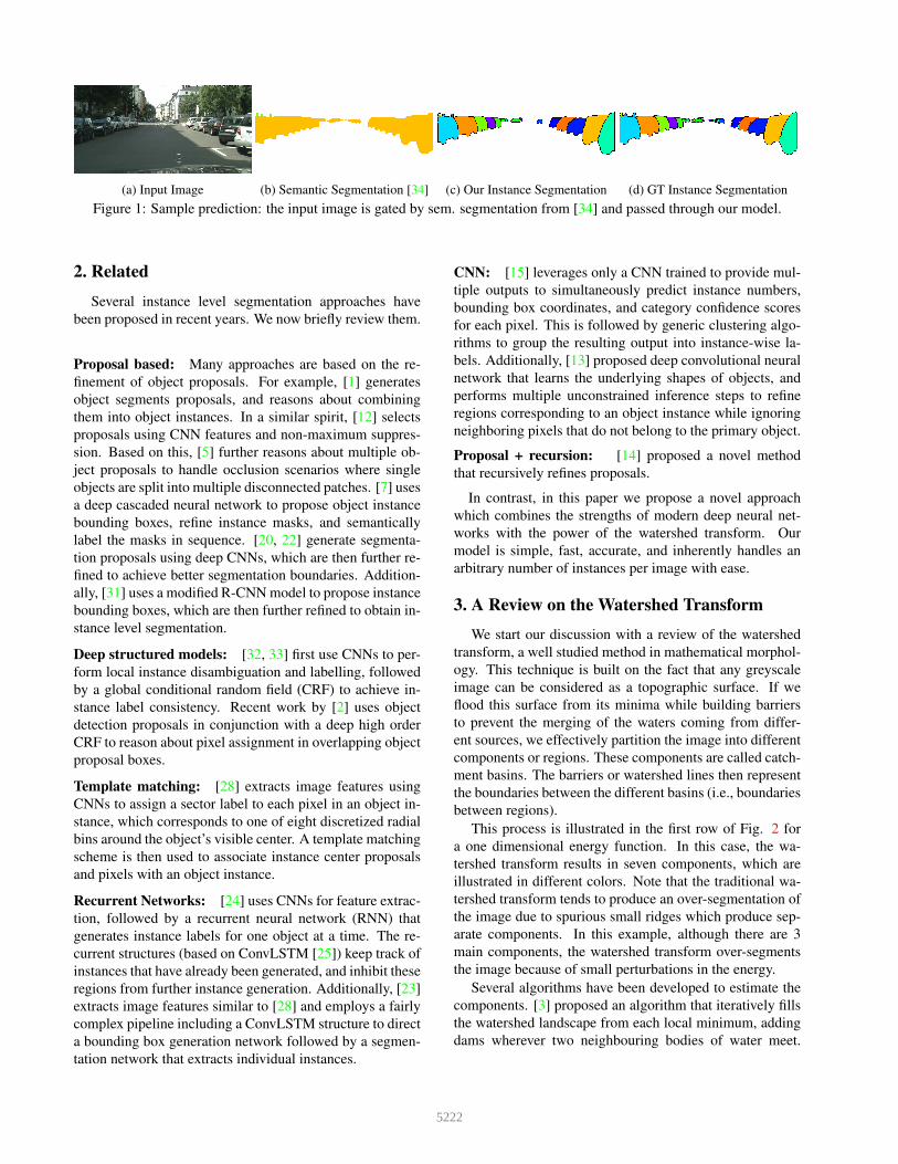
(a) Input Image (b) Semantic Segmentation [34] (c) Our Instance Segmentation (d) GT Instance Segmentation

Figure 1: Sample prediction: the input image is gated by sem. segmentation from [34] and passed through our model.

2. Related

Several instance level segmentation approaches have

been proposed in recent years. We now briefly review them.

Proposal based: Many approaches are based on the re-

finement of object proposals. For example, [1] generates

object segments proposals, and reasons about combining

them into object instances. In a similar spirit, [12] selects

proposals using CNN features and non-maximum suppres-

sion. Based on this, [5] further reasons about multiple ob-

ject proposals to handle occlusion scenarios where single

objects are split into multiple disconnected patches. [7] uses

a deep cascaded neural network to propose object instance

bounding boxes, refine instance masks, and semantically

label the masks in sequence. [20, 22] generate segmenta-

tion proposals using deep CNNs, which are then further re-

fined to achieve better segmentation boundaries. Addition-

ally, [31] uses a modified R-CNN model to propose instance

bounding boxes, which are then further refined to obtain in-

stance level segmentation.

Deep structured models: [32, 33] first use CNNs to per-

form local instance disambiguation and labelling, followed

by a global conditional random field (CRF) to achieve in-

stance label consistency. Recent work by [2] uses object

detection proposals in conjunction with a deep high order

CRF to reason about pixel assignment in overlapping object

proposal boxes.

Template matching: [28] extracts image features using

CNNs to assign a sector label to each pixel in an object in-

stance, which corresponds to one of eight discretized radial

bins around the object’s visible center. A template matching

scheme is then used to associate instance center proposals

and pixels with an object instance.

Recurrent Networks: [24] uses CNNs for feature extrac-

tion, followed by a recurrent neural network (RNN) that

generates instance labels for one object at a time. The re-

current structures (based on ConvLSTM [25]) keep track of

instances that have already been generated, and inhibit these

regions from further instance generation. Additionally, [23]

extracts image features similar to [28] and employs a fairly

complex pipeline including a ConvLSTM structure to direct

a bounding box generation network followed by a segmen-

tation network that extracts individual instances.

CNN: [15] leverages only a CNN trained to provide mul-

tiple outputs to simultaneously predict instance numbers,

bounding box coordinates, and category confidence scores

for each pixel. This is followed by generic clustering algo-

rithms to group the resulting output into instance-wise la-

bels. Additionally, [13] proposed deep convolutional neural

network that learns the underlying shapes of objects, and

performs multiple unconstrained inference steps to refine

regions corresponding to an object instance while ignoring

neighboring pixels that do not belong to the primary object.

Proposal + recursion: [14] proposed a novel method

that recursively refines proposals.

In contrast, in this paper we propose a novel approach

which combines the strengths of modern deep neural net-

works with the power of the watershed transform. Our

model is simple, fast, accurate, and inherently handles an

arbitrary number of instances per image with ease.

3. A Review on the Watershed Transform

We start our discussion with a review of the watershed

transform, a well studied method in mathematical morphol-

ogy. This technique is built on the fact that any greyscale

image can be considered as a topographic surface. If we

flood this surface from its minima while building barriers

to prevent the merging of the waters coming from differ-

ent sources, we effectively partition the image into different

components or regions. These components are called catch-

ment basins. The barriers or watershed lines then represent

the boundaries between the different basins (i.e., boundaries

between regions).

This process is illustrated in the first row of Fig. 2 for

a one dimensional energy function. In this case, the wa-

tershed transform results in seven components, which are

illustrated in different colors. Note that the traditional wa-

tershed transform tends to produce an over-segmentation of

the image due to spurious small ridges which produce sep-

arate components. In this example, although there are 3

main components, the watershed transform over-segments

the image because of small perturbations in the energy.

Several algorithms have been developed to estimate the

components. [3] proposed an algorithm that iteratively fills

the watershed landscape from each local minimum, adding

dams wherever two neighbouring bodies of water meet.

5222

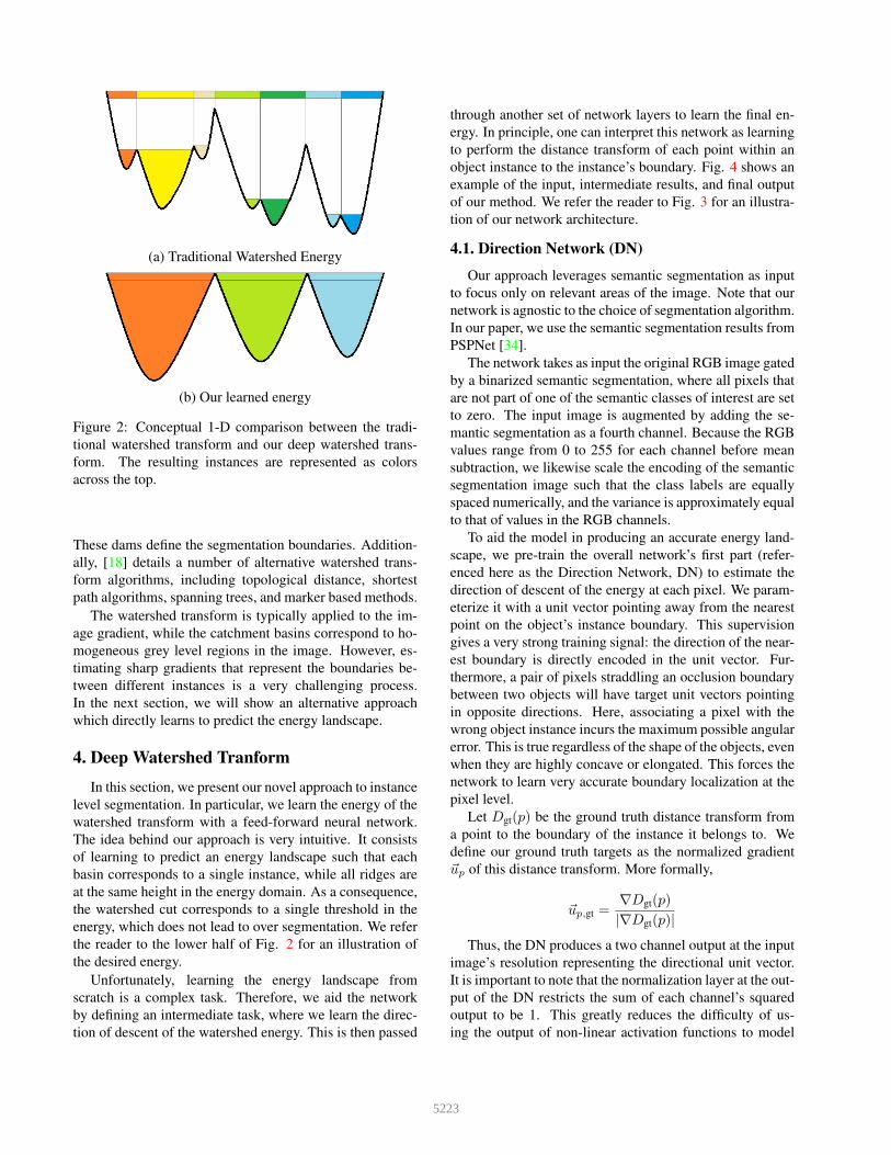
(a) Traditional Watershed Energy

(b) Our learned energy

Figure 2: Conceptual 1-D comparison between the tradi-

tional watershed transform and our deep watershed trans-

form. The resulting instances are represented as colors

across the top.

These dams define the segmentation boundaries. Addition-

ally, [18] details a number of alternative watershed trans-

form algorithms, including topological distance, shortest

path algorithms, spanning trees, and marker based methods.

The watershed transform is typically applied to the im-

age gradient, while the catchment basins correspond to ho-

mogeneous grey level regions in the image. However, es-

timating sharp gradients that represent the boundaries be-

tween different instances is a very challenging process.

In the next section, we will show an alternative approach

which directly learns to predict the energy landscape.

4. Deep Watershed Tranform

In this section, we present our novel approach to instance

level segmentation. In particular, we learn the energy of the

watershed transform with a feed-forward neural network.

The idea behind our approach is very intuitive. It consists

of learning to predict an energy landscape such that each

basin corresponds to a single instance, while all ridges are

at the same height in the energy domain. As a consequence,

the watershed cut corresponds to a single threshold in the

energy, which does not lead to over segmentation. We refer

the reader to the lower half of Fig. 2 for an illustration of

the desired energy.

Unfortunately, learning the energy landscape from

scratch is a complex task. Therefore, we aid the network

by defining an intermediate task, where we learn the direc-

tion of descent of the watershed energy. This is then passed

through another set of network layers to learn the final en-

ergy. In principle, one can interpret this network as learning

to perform the distance transform of each point within an

object instance to the instance’s boundary. Fig. 4 shows an

example of the input, intermediate results, and final output

of our method. We refer the reader to Fig. 3 for an illustra-

tion of our network architecture.

4.1. Direction Network (DN)

Our approach leverages semantic segmentation as input

to focus only on relevant areas of the image. Note that our

network is agnostic to the choice of segmentation algorithm.

In our paper, we use the semantic segmentation results from

PSPNet [34].

The network takes as input the original RGB image gated

by a binarized semantic segmentation, where all pixels that

are not part of one of the semantic classes of interest are set

to zero. The input image is augmented by adding the se-

mantic segmentation as a fourth channel. Because the RGB

values range from 0 to 255 for each channel before mean

subtraction, we likewise scale the encoding of the semantic

segmentation image such that the class labels are equally

spaced numerically, and the variance is approximately equal

to that of values in the RGB channels.

To aid the model in producing an accurate energy land-

scape, we pre-train the overall network’s first part (refer-

enced here as the Direction Network, DN) to estimate the

direction of descent of the energy at each pixel. We param-

eterize it with a unit vector pointing away from the nearest

point on the object’s instance boundary. This supervision

gives a very strong training signal: the direction of the near-

est boundary is directly encoded in the unit vector. Fur-

thermore, a pair of pixels straddling an occlusion boundary

between two objects will have target unit vectors pointing

in opposite directions. Here, associating a pixel with the

wrong object instance incurs the maximum possible angular

error. This is true regardless of the shape of the objects, even

when they are highly concave or elongated. This forces the

network to learn very accurate boundary localization at the

pixel level.

Let Dgt(p) be the ground truth distance transform from

a point to the boundary of the instance it belongs to. We

define our ground truth targets as the normalized gradient

~up of this distance transform. More formally,

~up,gt =∇Dgt(p)

|∇Dgt(p)|

Thus, the DN produces a two channel output at the input

image’s resolution representing the directional unit vector.

It is important to note that the normalization layer at the out-

put of the DN restricts the sum of each channel’s squared

output to be 1. This greatly reduces the difficulty of us-

ing the output of non-linear activation functions to model

5223

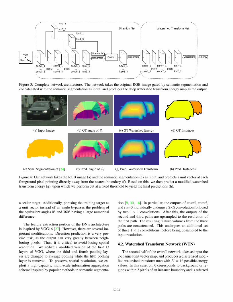
Figure 3: Complete network architecture. The network takes the original RGB image gated by semantic segmentation and

concatenated with the semantic segmentation as input, and produces the deep watershed transform energy map as the output.

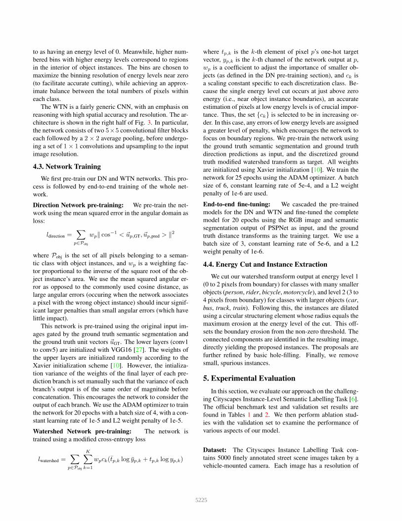
(a) Input Image (b) GT angle of ~up (c) GT Watershed Energy (d) GT Instances

(e) Sem. Segmentation of [34] (f) Pred. angle of ~up (g) Pred. Watershed Transform (h) Pred. Instances

Figure 4: Our network takes the RGB image (a) and the semantic segmentation (e) as input, and predicts a unit vector at each

foreground pixel pointing directly away from the nearest boundary (f). Based on this, we then predict a modified watershed

transform energy (g), upon which we perform cut at a fixed threshold to yield the final predictions (h).

a scalar target. Additionally, phrasing the training target as

a unit vector instead of an angle bypasses the problem of

the equivalent angles 0◦ and 360◦ having a large numerical

difference.

The feature extraction portion of the DN’s architecture

is inspired by VGG16 [27]. However, there are several im-

portant modifications. Direction prediction is a very pre-

cise task, as the output can vary greatly between neigh-

boring pixels. Thus, it is critical to avoid losing spatial

resolution. We utilize a modified version of the first 13

layers of VGG, where the third and fourth pooling lay-

ers are changed to average pooling while the fifth pooling

layer is removed. To preserve spatial resolution, we ex-

ploit a high-capacity, multi-scale information aggregation

scheme inspired by popular methods in semantic segmenta-

tion [9, 30, 16]. In particular, the outputs of conv3, conv4,

and conv5 individually undergo a 5×5 convolution followed

by two 1 × 1 convolutions. After this, the outputs of the

second and third paths are upsampled to the resolution of

the first path. The resulting feature volumes from the three

paths are concatenated. This undergoes an additional set

of three 1 × 1 convolutions, before being upsampled to the

input resolution.

4.2. Watershed Transform Network (WTN)

The second half of the overall network takes as input the

2-channel unit vector map, and produces a discretized modi-

fied watershed transform map with K = 16 possible energy

values. In this case, bin 0 corresponds to background or re-

gions within 2 pixels of an instance boundary and is referred

5224

to as having an energy level of 0. Meanwhile, higher num-

bered bins with higher energy levels correspond to regions

in the interior of object instances. The bins are chosen to

maximize the binning resolution of energy levels near zero

(to facilitate accurate cutting), while achieving an approx-

imate balance between the total numbers of pixels within

each class.

The WTN is a fairly generic CNN, with an emphasis on

reasoning with high spatial accuracy and resolution. The ar-

chitecture is shown in the right half of Fig. 3. In particular,

the network consists of two 5×5 convolutional filter blocks

each followed by a 2 × 2 average pooling, before undergo-

ing a set of 1× 1 convolutions and upsampling to the input

image resolution.

4.3. Network Training

We first pre-train our DN and WTN networks. This pro-

cess is followed by end-to-end training of the whole net-

work.

Direction Network pre-training: We pre-train the net-

work using the mean squared error in the angular domain as

loss:

ldirection =∑

p∈Pobj

wp‖ cos−1 < ~up,GT, ~up,pred > ‖2

where Pobj is the set of all pixels belonging to a seman-

tic class with object instances, and wp is a weighting fac-

tor proportional to the inverse of the square root of the ob-

ject instance’s area. We use the mean squared angular er-

ror as opposed to the commonly used cosine distance, as

large angular errors (occuring when the network associates

a pixel with the wrong object instance) should incur signif-

icant larger penalties than small angular errors (which have

little impact).

This network is pre-trained using the original input im-

ages gated by the ground truth semantic segmentation and

the ground truth unit vectors ~uGT. The lower layers (conv1

to conv5) are initialized with VGG16 [27]. The weights of

the upper layers are initialized randomly according to the

Xavier initialization scheme [10]. However, the intializa-

tion variance of the weights of the final layer of each pre-

diction branch is set manually such that the variance of each

branch’s output is of the same order of magnitude before

concatenation. This encourages the network to consider the

output of each branch. We use the ADAM optimizer to train

the network for 20 epochs with a batch size of 4, with a con-

stant learning rate of 1e-5 and L2 weight penalty of 1e-5.

Watershed Network pre-training: The network is

trained using a modified cross-entropy loss

lwatershed =∑

p∈Pobj

K∑

k=1

wpck(tp,k log yp,k + tp,k log yp,k)

where tp,k is the k-th element of pixel p’s one-hot target

vector, yp,k is the k-th channel of the network output at p,

wp is a coefficient to adjust the importance of smaller ob-

jects (as defined in the DN pre-training section), and ck is

a scaling constant specific to each discretization class. Be-

cause the single energy level cut occurs at just above zero

energy (i.e., near object instance boundaries), an accurate

estimation of pixels at low energy levels is of crucial impor-

tance. Thus, the set {ck} is selected to be in increasing or-

der. In this case, any errors of low energy levels are assigned

a greater level of penalty, which encourages the network to

focus on boundary regions. We pre-train the network using

the ground truth semantic segmentation and ground truth

direction predictions as input, and the discretized ground

truth modified watershed transform as target. All weights

are initialized using Xavier initialization [10]. We train the

network for 25 epochs using the ADAM optimizer. A batch

size of 6, constant learning rate of 5e-4, and a L2 weight

penalty of 1e-6 are used.

End-to-end fine-tuning: We cascaded the pre-trained

models for the DN and WTN and fine-tuned the complete

model for 20 epochs using the RGB image and semantic

segmentation output of PSPNet as input, and the ground

truth distance transforms as the training target. We use a

batch size of 3, constant learning rate of 5e-6, and a L2

weight penalty of 1e-6.

4.4. Energy Cut and Instance Extraction

We cut our watershed transform output at energy level 1

(0 to 2 pixels from boundary) for classes with many smaller

objects (person, rider, bicycle, motorcycle), and level 2 (3 to

4 pixels from boundary) for classes with larger objects (car,

bus, truck, train). Following this, the instances are dilated

using a circular structuring element whose radius equals the

maximum erosion at the energy level of the cut. This off-

sets the boundary erosion from the non-zero threshold. The

connected components are identified in the resulting image,

directly yielding the proposed instances. The proposals are

further refined by basic hole-filling. Finally, we remove

small, spurious instances.

5. Experimental Evaluation

In this section, we evaluate our approach on the challeng-

ing Cityscapes Instance-Level Semantic Labelling Task [6].

The official benchmark test and validation set results are

found in Tables 1 and 2. We then perform ablation stud-

ies with the validation set to examine the performance of

various aspects of our model.

Dataset: The Cityscapes Instance Labelling Task con-

tains 5000 finely annotated street scene images taken by a

vehicle-mounted camera. Each image has a resolution of

5225

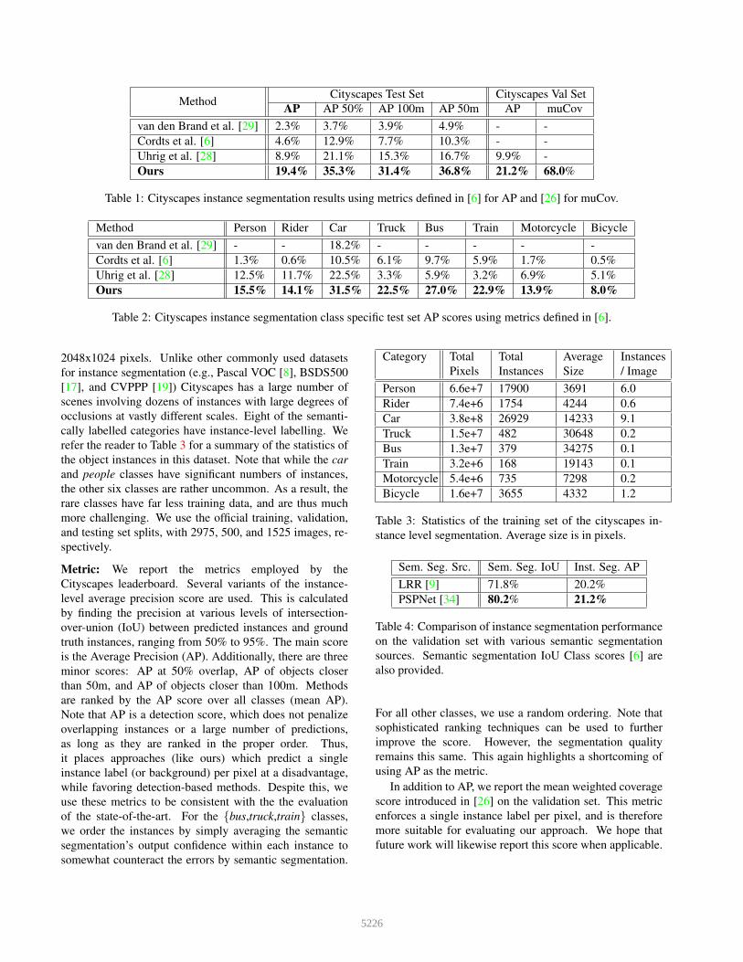
MethodCityscapes Test Set Cityscapes Val Set

AP AP 50% AP 100m AP 50m AP muCov

van den Brand et al. [29] 2.3% 3.7% 3.9% 4.9% - -

Cordts et al. [6] 4.6% 12.9% 7.7% 10.3% - -

Uhrig et al. [28] 8.9% 21.1% 15.3% 16.7% 9.9% -

Ours 19.4% 35.3% 31.4% 36.8% 21.2% 68.0%

Table 1: Cityscapes instance segmentation results using metrics defined in [6] for AP and [26] for muCov.

Method Person Rider Car Truck Bus Train Motorcycle Bicycle

van den Brand et al. [29] - - 18.2% - - - - -

Cordts et al. [6] 1.3% 0.6% 10.5% 6.1% 9.7% 5.9% 1.7% 0.5%

Uhrig et al. [28] 12.5% 11.7% 22.5% 3.3% 5.9% 3.2% 6.9% 5.1%

Ours 15.5% 14.1% 31.5% 22.5% 27.0% 22.9% 13.9% 8.0%

Table 2: Cityscapes instance segmentation class specific test set AP scores using metrics defined in [6].

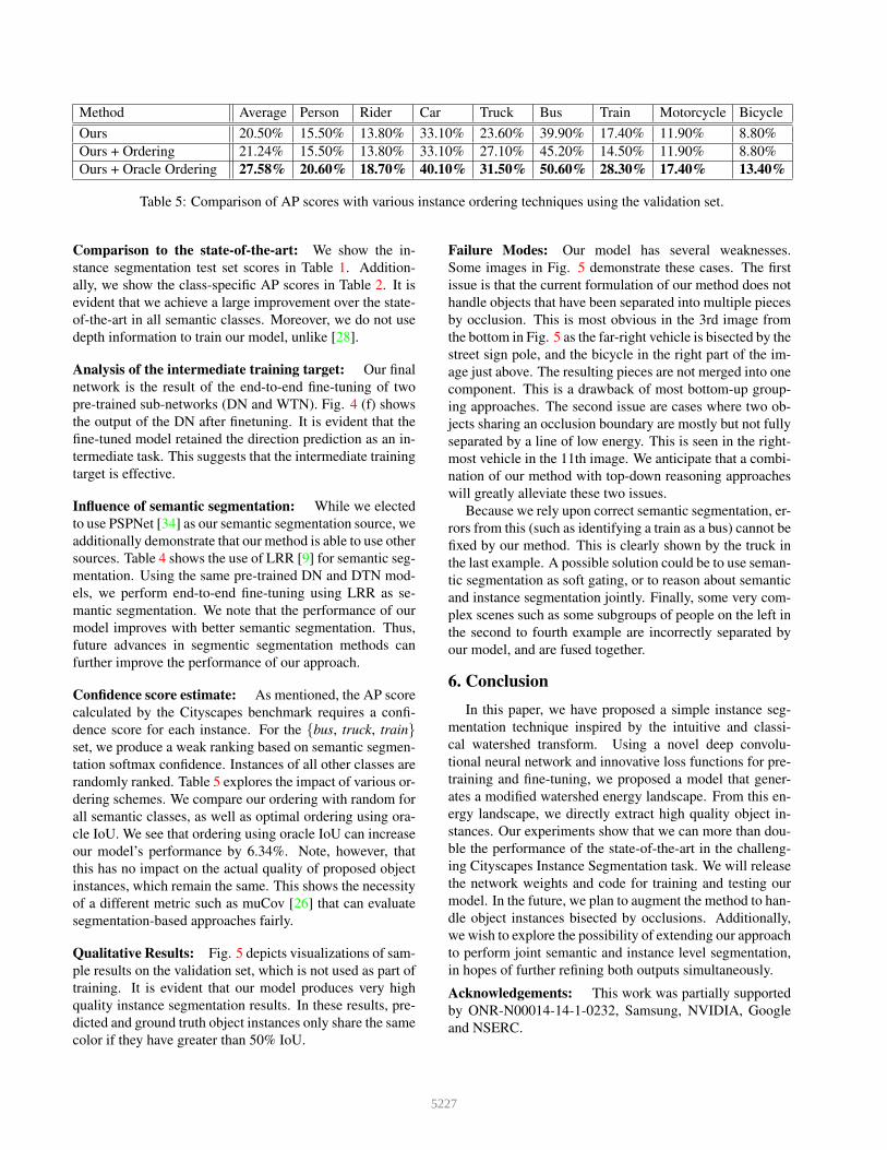
2048x1024 pixels. Unlike other commonly used datasets

for instance segmentation (e.g., Pascal VOC [8], BSDS500

[17], and CVPPP [19]) Cityscapes has a large number of

scenes involving dozens of instances with large degrees of

occlusions at vastly different scales. Eight of the semanti-

cally labelled categories have instance-level labelling. We

refer the reader to Table 3 for a summary of the statistics of

the object instances in this dataset. Note that while the car

and people classes have significant numbers of instances,

the other six classes are rather uncommon. As a result, the

rare classes have far less training data, and are thus much

more challenging. We use the official training, validation,

and testing set splits, with 2975, 500, and 1525 images, re-

spectively.

Metric: We report the metrics employed by the

Cityscapes leaderboard. Several variants of the instance-

level average precision score are used. This is calculated

by finding the precision at various levels of intersection-

over-union (IoU) between predicted instances and ground

truth instances, ranging from 50% to 95%. The main score

is the Average Precision (AP). Additionally, there are three

minor scores: AP at 50% overlap, AP of objects closer

than 50m, and AP of objects closer than 100m. Methods

are ranked by the AP score over all classes (mean AP).

Note that AP is a detection score, which does not penalize

overlapping instances or a large number of predictions,

as long as they are ranked in the proper order. Thus,

it places approaches (like ours) which predict a single

instance label (or background) per pixel at a disadvantage,

while favoring detection-based methods. Despite this, we

use these metrics to be consistent with the the evaluation

of the state-of-the-art. For the {bus,truck,train} classes,

we order the instances by simply averaging the semantic

segmentation’s output confidence within each instance to

somewhat counteract the errors by semantic segmentation.

Category Total

Pixels

Total

Instances

Average

Size

Instances

/ Image

Person 6.6e+7 17900 3691 6.0

Rider 7.4e+6 1754 4244 0.6

Car 3.8e+8 26929 14233 9.1

Truck 1.5e+7 482 30648 0.2

Bus 1.3e+7 379 34275 0.1

Train 3.2e+6 168 19143 0.1

Motorcycle 5.4e+6 735 7298 0.2

Bicycle 1.6e+7 3655 4332 1.2

Table 3: Statistics of the training set of the cityscapes in-

stance level segmentation. Average size is in pixels.

Sem. Seg. Src. Sem. Seg. IoU Inst. Seg. AP

LRR [9] 71.8% 20.2%

PSPNet [34] 80.2% 21.2%

Table 4: Comparison of instance segmentation performance

on the validation set with various semantic segmentation

sources. Semantic segmentation IoU Class scores [6] are

also provided.

For all other classes, we use a random ordering. Note that

sophisticated ranking techniques can be used to further

improve the score. However, the segmentation quality

remains this same. This again highlights a shortcoming of

using AP as the metric.

In addition to AP, we report the mean weighted coverage

score introduced in [26] on the validation set. This metric

enforces a single instance label per pixel, and is therefore

more suitable for evaluating our approach. We hope that

future work will likewise report this score when applicable.

5226

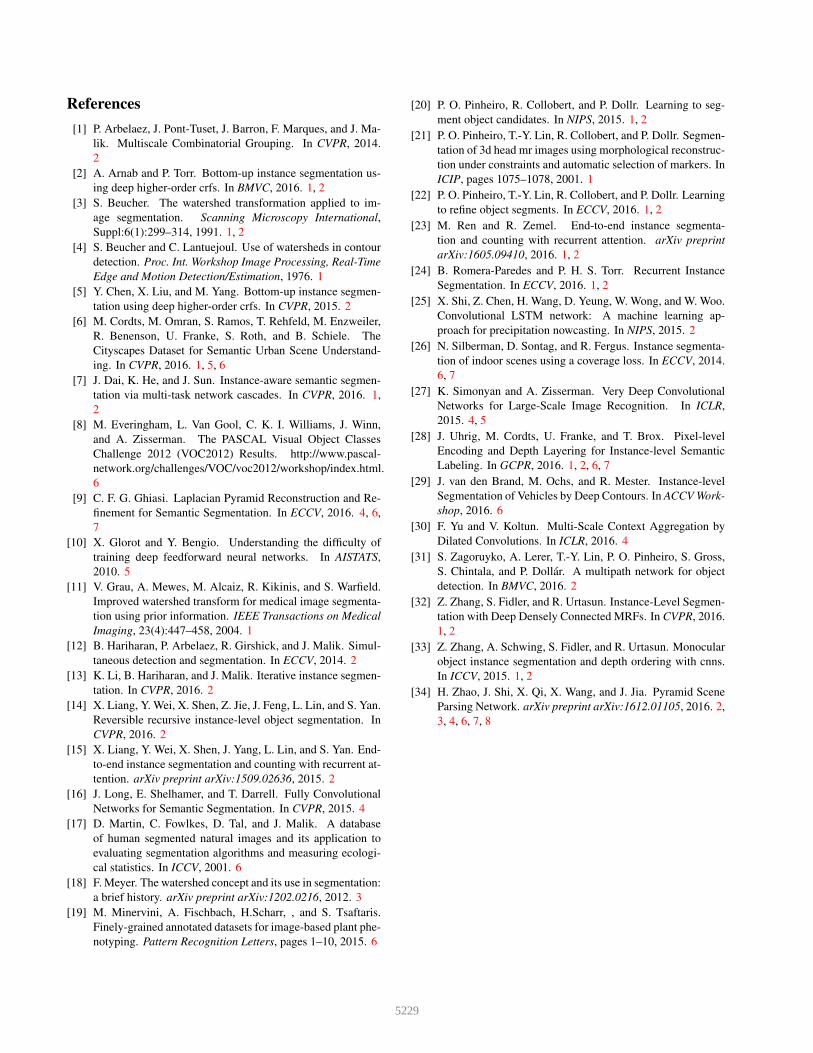
Method Average Person Rider Car Truck Bus Train Motorcycle Bicycle

Ours 20.50% 15.50% 13.80% 33.10% 23.60% 39.90% 17.40% 11.90% 8.80%

Ours + Ordering 21.24% 15.50% 13.80% 33.10% 27.10% 45.20% 14.50% 11.90% 8.80%

Ours + Oracle Ordering 27.58% 20.60% 18.70% 40.10% 31.50% 50.60% 28.30% 17.40% 13.40%

Table 5: Comparison of AP scores with various instance ordering techniques using the validation set.

Comparison to the state-of-the-art: We show the in-

stance segmentation test set scores in Table 1. Addition-

ally, we show the class-specific AP scores in Table 2. It is

evident that we achieve a large improvement over the state-

of-the-art in all semantic classes. Moreover, we do not use

depth information to train our model, unlike [28].

Analysis of the intermediate training target: Our final

network is the result of the end-to-end fine-tuning of two

pre-trained sub-networks (DN and WTN). Fig. 4 (f) shows

the output of the DN after finetuning. It is evident that the

fine-tuned model retained the direction prediction as an in-

termediate task. This suggests that the intermediate training

target is effective.

Influence of semantic segmentation: While we elected

to use PSPNet [34] as our semantic segmentation source, we

additionally demonstrate that our method is able to use other

sources. Table 4 shows the use of LRR [9] for semantic seg-

mentation. Using the same pre-trained DN and DTN mod-

els, we perform end-to-end fine-tuning using LRR as se-

mantic segmentation. We note that the performance of our

model improves with better semantic segmentation. Thus,

future advances in segmentic segmentation methods can

further improve the performance of our approach.

Confidence score estimate: As mentioned, the AP score

calculated by the Cityscapes benchmark requires a confi-

dence score for each instance. For the {bus, truck, train}set, we produce a weak ranking based on semantic segmen-

tation softmax confidence. Instances of all other classes are

randomly ranked. Table 5 explores the impact of various or-

dering schemes. We compare our ordering with random for

all semantic classes, as well as optimal ordering using ora-

cle IoU. We see that ordering using oracle IoU can increase

our model’s performance by 6.34%. Note, however, that

this has no impact on the actual quality of proposed object

instances, which remain the same. This shows the necessity

of a different metric such as muCov [26] that can evaluate

segmentation-based approaches fairly.

Qualitative Results: Fig. 5 depicts visualizations of sam-

ple results on the validation set, which is not used as part of

training. It is evident that our model produces very high

quality instance segmentation results. In these results, pre-

dicted and ground truth object instances only share the same

color if they have greater than 50% IoU.

Failure Modes: Our model has several weaknesses.

Some images in Fig. 5 demonstrate these cases. The first

issue is that the current formulation of our method does not

handle objects that have been separated into multiple pieces

by occlusion. This is most obvious in the 3rd image from

the bottom in Fig. 5 as the far-right vehicle is bisected by the

street sign pole, and the bicycle in the right part of the im-

age just above. The resulting pieces are not merged into one

component. This is a drawback of most bottom-up group-

ing approaches. The second issue are cases where two ob-

jects sharing an occlusion boundary are mostly but not fully

separated by a line of low energy. This is seen in the right-

most vehicle in the 11th image. We anticipate that a combi-

nation of our method with top-down reasoning approaches

will greatly alleviate these two issues.

Because we rely upon correct semantic segmentation, er-

rors from this (such as identifying a train as a bus) cannot be

fixed by our method. This is clearly shown by the truck in

the last example. A possible solution could be to use seman-

tic segmentation as soft gating, or to reason about semantic

and instance segmentation jointly. Finally, some very com-

plex scenes such as some subgroups of people on the left in

the second to fourth example are incorrectly separated by

our model, and are fused together.

6. Conclusion

In this paper, we have proposed a simple instance seg-

mentation technique inspired by the intuitive and classi-

cal watershed transform. Using a novel deep convolu-

tional neural network and innovative loss functions for pre-

training and fine-tuning, we proposed a model that gener-

ates a modified watershed energy landscape. From this en-

ergy landscape, we directly extract high quality object in-

stances. Our experiments show that we can more than dou-

ble the performance of the state-of-the-art in the challeng-

ing Cityscapes Instance Segmentation task. We will release

the network weights and code for training and testing our

model. In the future, we plan to augment the method to han-

dle object instances bisected by occlusions. Additionally,

we wish to explore the possibility of extending our approach

to perform joint semantic and instance level segmentation,

in hopes of further refining both outputs simultaneously.

Acknowledgements: This work was partially supported

by ONR-N00014-14-1-0232, Samsung, NVIDIA, Google

and NSERC.

5227

(a) Input Image (b) Sem. Segmentation [34] (c) Our Instance Segmentation (d) GT Instance Segmentation

Figure 5: Sample output of our model on the validation set. Note that predicted object instances and ground truth object

instances are only given the same color if they have over 50% IoU.

5228

References

[1] P. Arbelaez, J. Pont-Tuset, J. Barron, F. Marques, and J. Ma-

lik. Multiscale Combinatorial Grouping. In CVPR, 2014.

2

[2] A. Arnab and P. Torr. Bottom-up instance segmentation us-

ing deep higher-order crfs. In BMVC, 2016. 1, 2

[3] S. Beucher. The watershed transformation applied to im-

age segmentation. Scanning Microscopy International,

Suppl:6(1):299–314, 1991. 1, 2

[4] S. Beucher and C. Lantuejoul. Use of watersheds in contour

detection. Proc. Int. Workshop Image Processing, Real-Time

Edge and Motion Detection/Estimation, 1976. 1

[5] Y. Chen, X. Liu, and M. Yang. Bottom-up instance segmen-

tation using deep higher-order crfs. In CVPR, 2015. 2

[6] M. Cordts, M. Omran, S. Ramos, T. Rehfeld, M. Enzweiler,

R. Benenson, U. Franke, S. Roth, and B. Schiele. The

Cityscapes Dataset for Semantic Urban Scene Understand-

ing. In CVPR, 2016. 1, 5, 6

[7] J. Dai, K. He, and J. Sun. Instance-aware semantic segmen-

tation via multi-task network cascades. In CVPR, 2016. 1,

2

[8] M. Everingham, L. Van Gool, C. K. I. Williams, J. Winn,

and A. Zisserman. The PASCAL Visual Object Classes

Challenge 2012 (VOC2012) Results. http://www.pascal-

network.org/challenges/VOC/voc2012/workshop/index.html.

6

[9] C. F. G. Ghiasi. Laplacian Pyramid Reconstruction and Re-

finement for Semantic Segmentation. In ECCV, 2016. 4, 6,

7

[10] X. Glorot and Y. Bengio. Understanding the difficulty of

training deep feedforward neural networks. In AISTATS,

2010. 5

[11] V. Grau, A. Mewes, M. Alcaiz, R. Kikinis, and S. Warfield.

Improved watershed transform for medical image segmenta-

tion using prior information. IEEE Transactions on Medical

Imaging, 23(4):447–458, 2004. 1

[12] B. Hariharan, P. Arbelaez, R. Girshick, and J. Malik. Simul-

taneous detection and segmentation. In ECCV, 2014. 2

[13] K. Li, B. Hariharan, and J. Malik. Iterative instance segmen-

tation. In CVPR, 2016. 2

[14] X. Liang, Y. Wei, X. Shen, Z. Jie, J. Feng, L. Lin, and S. Yan.

Reversible recursive instance-level object segmentation. In

CVPR, 2016. 2

[15] X. Liang, Y. Wei, X. Shen, J. Yang, L. Lin, and S. Yan. End-

to-end instance segmentation and counting with recurrent at-

tention. arXiv preprint arXiv:1509.02636, 2015. 2

[16] J. Long, E. Shelhamer, and T. Darrell. Fully Convolutional

Networks for Semantic Segmentation. In CVPR, 2015. 4

[17] D. Martin, C. Fowlkes, D. Tal, and J. Malik. A database

of human segmented natural images and its application to

evaluating segmentation algorithms and measuring ecologi-

cal statistics. In ICCV, 2001. 6

[18] F. Meyer. The watershed concept and its use in segmentation:

a brief history. arXiv preprint arXiv:1202.0216, 2012. 3

[19] M. Minervini, A. Fischbach, H.Scharr, , and S. Tsaftaris.

Finely-grained annotated datasets for image-based plant phe-

notyping. Pattern Recognition Letters, pages 1–10, 2015. 6

[20] P. O. Pinheiro, R. Collobert, and P. Dollr. Learning to seg-

ment object candidates. In NIPS, 2015. 1, 2

[21] P. O. Pinheiro, T.-Y. Lin, R. Collobert, and P. Dollr. Segmen-

tation of 3d head mr images using morphological reconstruc-

tion under constraints and automatic selection of markers. In

ICIP, pages 1075–1078, 2001. 1

[22] P. O. Pinheiro, T.-Y. Lin, R. Collobert, and P. Dollr. Learning

to refine object segments. In ECCV, 2016. 1, 2

[23] M. Ren and R. Zemel. End-to-end instance segmenta-

tion and counting with recurrent attention. arXiv preprint

arXiv:1605.09410, 2016. 1, 2

[24] B. Romera-Paredes and P. H. S. Torr. Recurrent Instance

Segmentation. In ECCV, 2016. 1, 2

[25] X. Shi, Z. Chen, H. Wang, D. Yeung, W. Wong, and W. Woo.

Convolutional LSTM network: A machine learning ap-

proach for precipitation nowcasting. In NIPS, 2015. 2

[26] N. Silberman, D. Sontag, and R. Fergus. Instance segmenta-

tion of indoor scenes using a coverage loss. In ECCV, 2014.

6, 7

[27] K. Simonyan and A. Zisserman. Very Deep Convolutional

Networks for Large-Scale Image Recognition. In ICLR,

2015. 4, 5

[28] J. Uhrig, M. Cordts, U. Franke, and T. Brox. Pixel-level

Encoding and Depth Layering for Instance-level Semantic

Labeling. In GCPR, 2016. 1, 2, 6, 7

[29] J. van den Brand, M. Ochs, and R. Mester. Instance-level

Segmentation of Vehicles by Deep Contours. In ACCV Work-

shop, 2016. 6

[30] F. Yu and V. Koltun. Multi-Scale Context Aggregation by

Dilated Convolutions. In ICLR, 2016. 4

[31] S. Zagoruyko, A. Lerer, T.-Y. Lin, P. O. Pinheiro, S. Gross,

S. Chintala, and P. Dollar. A multipath network for object

detection. In BMVC, 2016. 2

[32] Z. Zhang, S. Fidler, and R. Urtasun. Instance-Level Segmen-

tation with Deep Densely Connected MRFs. In CVPR, 2016.

1, 2

[33] Z. Zhang, A. Schwing, S. Fidler, and R. Urtasun. Monocular

object instance segmentation and depth ordering with cnns.

In ICCV, 2015. 1, 2

[34] H. Zhao, J. Shi, X. Qi, X. Wang, and J. Jia. Pyramid Scene

Parsing Network. arXiv preprint arXiv:1612.01105, 2016. 2,

3, 4, 6, 7, 8

5229