DeepNAT: Deep Convolutional Neural Network for Segmenting Neuroanatomy

Christian Wachingera∗, Martin Reuterb,c, Tassilo Kleind

aDepartment of Child and Adolescent Psychiatry, Psychosomatic and Psychotherapy, Ludwig-Maximilian-University, Munich, GermanybAthinoula A. Martinos Center for Biomedical Imaging, Massachusetts General Hospital, Harvard Medical School, Boston, MA, USA

cComputer Science and Artificial Intelligence Laboratory, Massachusetts Institute of Technology, Cambridge, MA, USAdSAP SE, Berlin, Germany

Abstract

We introduce DeepNAT, a 3D Deep convolutional neural network for the automatic segmentation of NeuroAnaTomy inT1-weighted magnetic resonance images. DeepNAT is an end-to-end learning-based approach to brain segmentation thatjointly learns an abstract feature representation and a multi-class classification. We propose a 3D patch-based approach,where we do not only predict the center voxel of the patch but also neighbors, which is formulated as multi-task learning.To address a class imbalance problem, we arrange two networks hierarchically, where the first one separates foregroundfrom background, and the second one identifies 25 brain structures on the foreground. Since patches lack spatialcontext, we augment them with coordinates. To this end, we introduce a novel intrinsic parameterization of the brainvolume, formed by eigenfunctions of the Laplace-Beltrami operator. As network architecture, we use three convolutionallayers with pooling, batch normalization, and non-linearities, followed by fully connected layers with dropout. The finalsegmentation is inferred from the probabilistic output of the network with a 3D fully connected conditional random field,which ensures label agreement between close voxels. The roughly 2.7 million parameters in the network are learned withstochastic gradient descent. Our results show that DeepNAT compares favorably to state-of-the-art methods. Finally,the purely learning-based method may have a high potential for the adaptation to young, old, or diseased brains byfine-tuning the pre-trained network with a small training sample on the target application, where the availability oflarger datasets with manual annotations may boost the overall segmentation accuracy in the future.

Keywords: Brain segmentation, deep learning, convolutional neural networks, multi-task learning, conditional randomfield

1. Introduction

The accurate segmentation of neuroanatomy forms thebasis for volume, thickness, and shape measurements frommagnetic resonance imaging (MRI). Such quantitativemeasurements are widely studied in neuroscience to trackstructural brain changes associated with aging and dis-ease. Additionally, they provide a vast phenotypic char-acterization of an individual and can serve as endophe-notypes for disease. Since the manual segmentation ofbrain MRI scans is time consuming, computational toolshave been developed to automatically reconstruct neu-roanatomy, which is particularly important for the vastlygrowing number of large-scale brain studies. One of themost commonly used software tools for whole brain seg-mentation is FreeSurfer (Fischl et al., 2002), which appliesan atlas-based segmentation strategy with deformable reg-istration. This seminal work encouraged research in atlas-based segmentation, with a focus on multi-atlas techniquesand label fusion strategies (Ashburner and Friston, 2005;

∗Corresponding Author. Address: Waltherstr. 23,81369 Munchen, Germany; Email: christian.wachinger@med.uni-muenchen.de

Pohl et al., 2006; Heckemann et al., 2006; Rohlfing et al.,2004, 2005; Svarer et al., 2005; Sabuncu et al., 2010; As-man and Landman, 2012; Wang et al., 2013b; Wachingerand Golland, 2014). A potential drawback of atlas-basedsegmentation approaches is the computation of a deforma-tion field between subjects, which involves regularizationconstraints to solve an ill-conditioned optimization prob-lem. Typically smoothness constraints are enforced, whichmay impede the correct spatial alignment of inter-subjectscans. Interestingly, the deformation field is only used forpropagating the segmentation and not of interest by itself.

Learning-based approaches without deformable registra-tion present an alternative avenue for image segmenta-tion, where the atlas with manual segmentations servesas training set for predicting the segmentation of a newscan. Directly predicting the segmentation of the entireimage is challenging because of the high dimensionality,i.e., the number of voxels, and the limited number of train-ing scans with manual segmentations. Instead, the prob-lem is reduced to predicting the label for small image re-gions, known as patches. Good segmentation performancewas reported for patch-based approaches following a non-local means strategy (Coupe et al., 2011; Rousseau et al.,

Preprint submitted to NeuroImage

arX

iv:1

702.

0819

2v1

[cs

.CV

] 2

7 Fe

b 20

17

2011), which is similar to a nearest neighbor search inpatch space. Alternative patch classification schemes havebeen proposed, e.g., random forests (Zikic et al., 2013).A potentially limiting factor of patch-based approaches isthat they operate on image intensities, where previous re-sults in pattern recognition suggest that it is less the clas-sifier but rather the representation that primarily impactsthe performance of a predictive model (Dickinson, 2009).In a recent study, a wide range of image features for imagesegmentation was compared and a significant improvementfor augmenting intensity patches with features was mea-sured (Wachinger et al., 2016).

While image features improve the segmentation, theyare handcrafted and may therefore not be optimal for theapplication. In contrast, neural networks autonomouslylearn representations that are optimal for the given task,without the need for manually defining features. Neu-ral nets therefore break the common paradigm of patch-based segmentation, which separates feature extractionand classification, and replaces it with an end-to-end learn-ing framework that starts with the image data and pre-dicts the anatomical label. Deep convolutional neural net-works (DCNN) have had ample success in computer vi-sion (Krizhevsky et al., 2012) and increasingly in medicalimaging (Brosch et al., 2014; Ciresan et al., 2013; Pra-soon et al., 2013; Roth et al., 2014; Zheng et al., 2015;Brosch et al., 2015; Zhang et al., 2015; Pereira et al., 2015).Applications in computer vision are typically on 2D im-ages, where 2D+t DCNNs were proposed for human actionrecognition (Ji et al., 2013). In medical applications, 2.5Dtechniques have been proposed (Prasoon et al., 2013; Rothet al., 2014). The three orthogonal planes are integrated inexisting DCNNs frameworks by setting the planes in theRGB channels. Difficulties in training 3D DCNNs havebeen reported (Prasoon et al., 2013; Roth et al., 2014),due to the increase in complexity by adding an additionaldimension. Yet, several articles describe successful appli-cations of 3D networks on medical images. Brosch et al.(2015) propose a 3D deep convolutional encoder for lesionsegmentation. Zheng et al. (2015) use a multi-layer percep-tron for landmark detection. Most related to our work isthe application of 3D convolutional neural networks, whichis currently limited to few layers and small input patches.Li et al. (2014) use a 3D CNN with one convolutional andone fully connected layer for the prediction of PET fromMRI on patches of 153. Brebisson and Montana (2015) usea combination of 2D and 3D inputs for whole brain seg-mentation. The network uses one convolutional layer and3D sub-volumes of size 133. The foreground mask, i.e., theregion that contains the labels of interest, is assumed tobe given, which is not the case for scans without manualsegmentation.

We propose a 3D deep convolutional network for brainsegmentation that has more layers and operates on largerpatches than existing 3D DCNNs, giving it the potential tomodel more complex relationships necessary for identifyingfine-grained brain structures. We use latest advances in

deep learning to initialize weights, to correct for internalcovariate shift, and to limit overfitting for training suchcomplex models. The main contributions in DeepNAT are:

• Multi-task learning: our network does not only pre-dict the center label of the patch but also the labelsin a small neighborhood, formulated in the DCNN asthe simultaneous training of multiple tasks

• Hierarchical segmentation: we propose a hierarchicallearning approach that first separates foreground frombackground and then subdivides the foreground into25 brain structures to account for the class imbalancestemming from the large background class

• Spectral coordinates: we introduce spectral coordi-nates as an intrinsic brain parameterization by com-puting eigenfunctions of the Laplace-Beltrami opera-tor on the brain mask, retaining context informationin patches

The output of DeepNAT is a probabilistic label map thatneeds to be discretized to obtain the final segmentation.Performing the discretization independently for each voxelcan result in spurious segmentation artifacts. Formulatingconstraints among voxels, e.g., with pairwise potentials ina random field can improve the final segmentation. Tra-ditionally, such constraints have only been imposed in asmall neighborhood due to computational concerns (Wanget al., 2013a). We use the efficient implementation of afully connected conditional random field (CRF) that es-tablishes pairwise potentials on all voxel pairs (Krahenbuhland Koltun, 2011), which was shown to substantially im-prove the segmentation. The fully connected CRF is usedin combination with DCNNs for natural image segmen-tation in DeepLab (Chen et al., 2015, 2016). It is alsoemployed for the segmentation of 2D medical images: Fuet al. (2016) segment vessels in 2D retinal images and Gaoet al. (2016) segment the lung in 2D CT slices. In con-trast to these approaches, we perform MAP inference ofthe CRF in 3D on the entire image domain to obtain thefinal brain segmentation.

2. Method

Given a novel image I, we aim to infer its segmenta-tion S based on training images I = {I1, . . . , In} withsegmentations S = {S1, . . . , Sn}. A probabilistic labelmap L = {L1, . . . , Lη} specifies the likelihood for eachbrain label l ∈ {1, . . . , η}

Ll(x) = p(S(x) = l|I; I,S). (1)

Let I(Nx) denote an image patch centered at location x,the likelihood in a patch-based segmentation approach is

Ll(x) = p(S(x) = l|I(Nx); I,S). (2)

2

MRI Foreground-­‐Background

Multi-­‐task   CNN

Segmentation

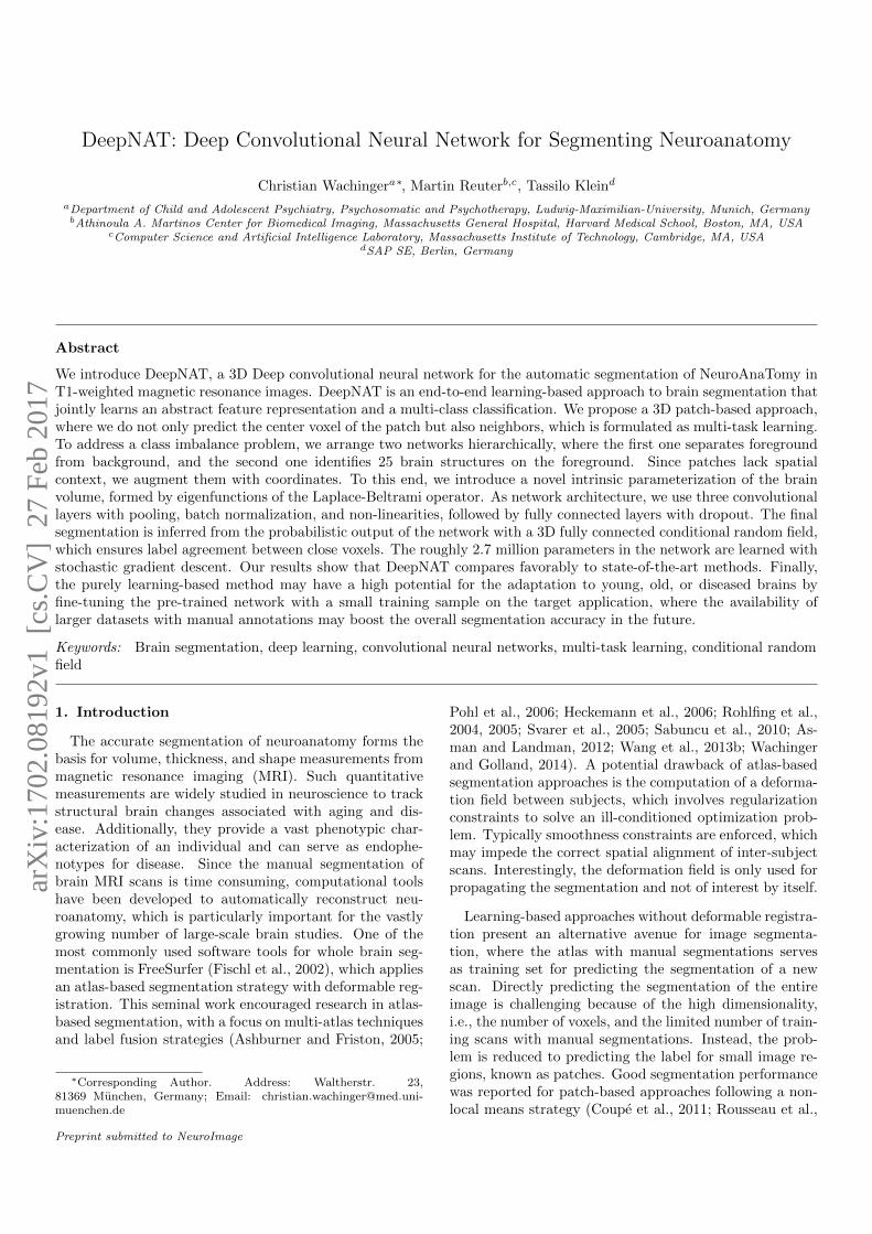
Multi-­‐task   CNN

Figure 1: Overview of the hierarchical segmentation with spectral coordinates. The first multi-task DCNN separates foreground frombackground on skull-stripped images; the second one identifies 25 brain structures on the foreground.

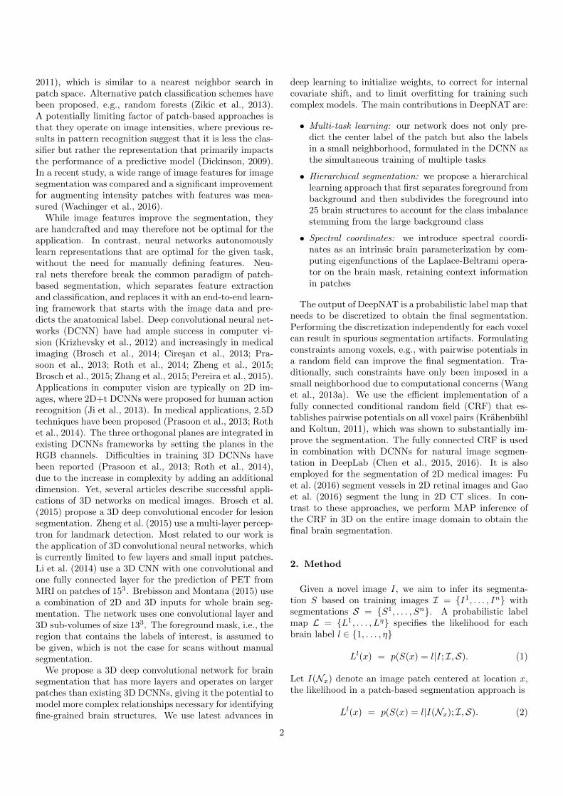
3D Multi-Task Network ArchitectureLayers Specification Layers Specification

1. Convolution 7× 7× 7× 32 10. Inner Product Neurons: 10242. ReLU 11. ReLU3. Max-Pooling Size: 2, Stride: 2 12. Dropout Rate: 0.54. Convolution 5× 5× 5× 64 13. Concatenation w/ coordinates5. Batch normalization 14. Inner Product Neurons: 5126. ReLU 15. Batch normalization7. Convolution 3× 3× 3× 64 16. ReLU8. Batch normalization 17. Dropout Rate: 0.59. ReLU Output: 1728 18. Inner Product (× tasks) Neurons: 2 / 25

Table 1: DeepNAT network architecture with convolutional (left) and fully connected (right) parts. The size of the input patch is 233. Thelast layer is replicated for multi-task learning according to the number of tasks. The cascaded networks are identical except for the numberof neurons in the last layer.

We estimate the likelihood by training a deep convolu-tional neural network, where the patch inference corre-sponds to multi-class classification. We skull strip the im-ages to focus the prediction on the brain mask; a brainscan from which the skull and other non-brain tissue likedura and eyes are removed.

2.1. Hierarchical Segmentation

Figure 1 illustrates the hierarchical approach for wholebrain segmentation in DeepNAT. In the first cascade, brainregions are classified into foreground and background. Theforeground consists of 25 major brain structures that are il-lustrated in Figure 7. The background is the region withinthe brain mask that is not part of the foreground. Datathat is classified as foreground undergoes the next cas-caded step to identify separate brain structures. Giventhe inherent class imbalance, the hierarchical segmenta-tion has the potential to perform better than a single-step classification, which classifies into brain regions aswell as background. Problems with a large backgroundclass have previously been noted for atlas-based segmen-tation (Wachinger and Golland, 2014). The background istypically represented by a large pool of data, while smallbrain structures are prone to being underrepresented. On

our data, we measured a foreground to background vol-ume ratio of about 2 to 1. The background is thereforesubstantially larger than any of the individual brain struc-tures on the foreground. As data augmentation allows onlyfor crude and poor compensation, the cascaded approachpresents a viable alternative.

2.2. Network Architecture

Multi-layer convolutional neural networks pioneeredby LeCun et al. (1989) have led to breakthrough results,constituting the state-of-the art technology for many chal-lenges such as ImageNet (Krizhevsky et al., 2012). Theunderlying idea is to create a deep hierarchical featurerepresentation that shares filter weights across the inputdomain. This allows for the robust modeling of complexrelationships while requiring a reduced number of param-eters, for which solutions can be obtained by stochasticgradient descent.

Table 1 lists the details of the DeepNAT network archi-tecture, where both networks (for each cascade) are iden-tical except for the number of neurons in the last layer (2and 25, respectively). The network consists of three con-volutional layers, where in each layer the filter masks areto be learned. A filter mask is specified by the spatial di-mension, e.g let@tokeneonedot, 5 × 5 × 5 and the number

3

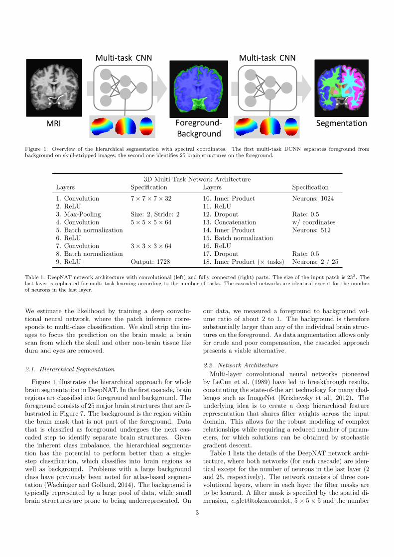
Layer Parameter calculation # Parameters Input Dimensionality Output Dimensionality

Convolution I 7× 7× 7× 1× 32 10,976 23× 23× 23× 1 17× 17× 17× 32Convolution II 5× 5× 5× 32× 64 256,000 9× 9× 9× 32 5× 5× 5× 64Convolution III 3× 3× 3× 64× 64 110,592 5× 5× 5× 64 3× 3× 3× 64Inner Product I 3× 3× 3× 64× 1024 1,769,472 3× 3× 3× 64 1024Inner Product II (1024 + 6)× 512 527,360 1030 512Inner Product III 512× 25 12,800 512 25

Table 2: The number of parameters to be learned at each of the convolutional and inner product layers of the network. The total number ofparameters is 2,687,200. We also state the input and output dimensionality of each of the layers, which provides insights about the internalrepresentation. Note that max-pooling operates before convolution II and that spatial coordinates are concatenated before inner product II.The list does not include bias parameters, which are negligible in size.

of filters to be used, e.g let@tokeneonedot, 64. Each filterextends to all of the input channels. As an example, thefilters are of size 5× 5× 5× 32 in the second convolution.The total number of free parameters to be estimated is thefilter size times the number of filters, so 5×5×5×32×64for the second convolution. Table 2 states the number ofparameters together with the input and output dimension-ality for each layer. Note that for 2D DCNNs the filtershave 3 dimensions, whereas for 3D DCNNs the filters have4 dimensions.

Each convolution is followed by a rectified linear unit(ReLU) (Hahnloser et al., 2003; Glorot et al., 2011), whichsupports the efficient training of the network with re-duced risk for vanishing gradient compared to other non-linearities. The aim of the convolutional part of the net-work is to reduce the dimensionality from the initial patchsize of 23 × 23 × 23 before entering the fully connectedstage. Although each convolution reduces the size, we usean additional max-pooling layer with stride two to arriveat a 33 block of neurons at the end of the convolutionalstage. The 33 block is an explicit design choice. A smaller23 block would cause a lack of localization, with the patchcenter being split into exterior blocks. A larger 43 blockwould dramatically increase the number of parameters atthe end of the convolutional stage, where most free param-eters occur at the intersection between convolutional andfully connected layers, see Table 2.

We use batch normalization at several layers in thenetwork to reduce the internal covariate shift (Ioffe andSzegedy, 2015). It accounts for the problem that the dis-tribution of each layer’s inputs changes during training, asthe parameters of the previous layers change, which is morepronounced in 3D networks. We further use two dropoutlayers, which randomly disable neurons in the network.This helps with the generalizability of the network by act-ing as a regularizer and mitigating overfitting. To resolvepotential location ambiguity, coordinates of the patchesare given to the network, see Sec. 2.4. This is achieved byconcatenating the image content after the first fully con-nected layer with the location information in layer 13. Inthe training stage, we compute the multinomial logisticloss as last layer, where the probability distribution overclasses is inferred from the last inner product layer with a

softmax.

For the initialization of the weights, we use the Xavieralgorithm that automatically determines the scale of ini-tialization based on the number of input and output neu-rons (Glorot and Bengio, 2010). This initialization sup-ports training deep networks without requiring per-layerpre-training because signals can reach deep into the net-work without shrinking or growing too much.

2.3. Multi-task Learning

In Eq.(2), we use an image patch to predict the tissuelabel of the center voxel. Performing this inference onthe entire image results in a single vote per voxel. Pre-vious results in patch-based segmentation have, however,demonstrated the advantage of propagating not only thecenter label but also neighboring labels (Rousseau et al.,2011). With such an approach, the voxel label is not onlyinferred from a single patch, but also from neighboringpatches. Rousseau et al. (2011) refer to this as the multi-point method in the context of non-local means segmen-tation. We propose to replicate the multi-point methodfor DCNN segmentation by employing multi-task learning.Instead of learning a single task, which predicts the centerlabel, we simultaneously learn multiple tasks, which pre-dict the center and surrounding neighborhood. The neigh-borhood size determines the number of tasks. While therehave been applications for deep multi-task learning (Yimet al., 2015; Luong et al., 2015), we are not aware of pre-vious applications for image segmentation.

We implement multi-task learning in the CDNN archi-tecture by replicating the last inner product layer (#18)according to the number of tasks. The increase in the num-ber of parameters to be learned is limited by this setup be-cause all tasks share the same network, except for last in-ner product layer that specializes on the task. Each task tpredicts the likelihood pt(S(xt) = l|I(Nx); I,S) for loca-tions xt in the neighborhood Mx centered around x. Wecompute the multi-task likelihood for the label by averag-ing likelihoods across tasks

Ll(x) =1

|Mx|∑

xt∈Mx

p(S(x) = l|I(Nxt); I,S). (3)

4

We experiment with 7 and 27 neighborhood systemsM forthe prediction, where the 7 neighborhood consists of the 6direct neighbors and the 27 neighborhood consists of thefull 33 region. From a different perspective, this approachof averaging among multiple predictions per voxel can alsobe seen as an ensemble method.

2.4. Spectral Brain Coordinates

A downside of patch-based segmentation techniques isthe loss of spatial context (Wachinger et al., 2016). Con-sidering the symmetry of the brain, it is easy to confusepatches across hemispheres. In addition, context providesvaluable information for structures with low tissue con-trast. To increase the spatial information, we augmentpatches with location information. Previous approacheshave, for instance, used Cartesian coordinates (Wachingeret al., 2014) or distances to centroids (Brebisson and Mon-tana, 2015). We propose spectral brain coordinates as analternative parameterization of the brain volume, whichwe obtain by computing eigenfunctions of the Laplace-Beltrami operator inside the 3D brain mask. Eigenfunc-tions of the cortex surface have previously been used forbrain matching (Lombaert et al., 2013b,a) and eigenvaluesas shape descriptors (Wachinger et al., 2015b). In contrast,we compute spectral coordinates on the solid (volume) anduse it as an intrinsic coordinate system for learning. Onthe brain mask, we solve the Laplacian eigenvalue problem

∆f = −λf (4)

with the Laplace-Beltrami operator ∆, eigenvalues λ andeigenfunctions f . We approximate the Laplace-Beltramioperator with the graph Laplacian (Chung, 1997). Theweights in the adjacency matrix W between two points iand j are set to 1 if both points are neighbors and withinthe brain mask, otherwise they are set to 0. This yields asparse matrix W . The Laplacian operator on a graph is

L = D −W Dii =∑j

Wij (5)

with the node degree matrix D.We compute the first three non-constant eigenvectors of

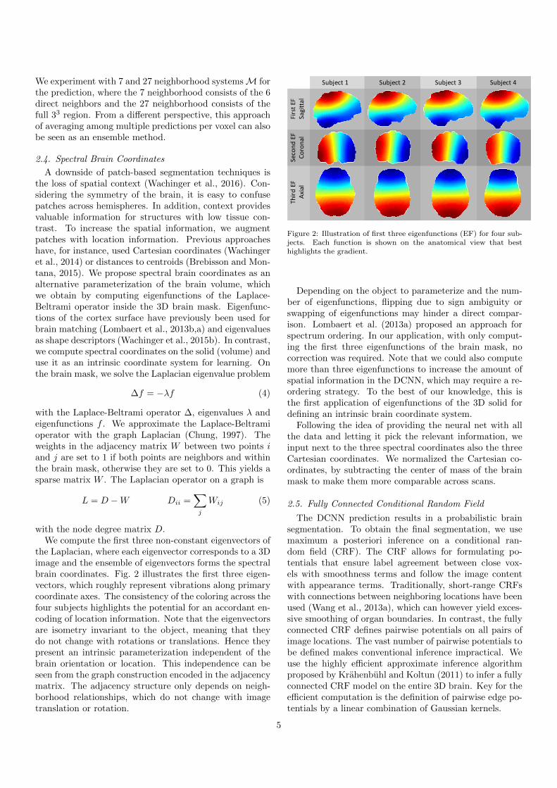
the Laplacian, where each eigenvector corresponds to a 3Dimage and the ensemble of eigenvectors forms the spectralbrain coordinates. Fig. 2 illustrates the first three eigen-vectors, which roughly represent vibrations along primarycoordinate axes. The consistency of the coloring across thefour subjects highlights the potential for an accordant en-coding of location information. Note that the eigenvectorsare isometry invariant to the object, meaning that theydo not change with rotations or translations. Hence theypresent an intrinsic parameterization independent of thebrain orientation or location. This independence can beseen from the graph construction encoded in the adjacencymatrix. The adjacency structure only depends on neigh-borhood relationships, which do not change with imagetranslation or rotation.

Subject  1 Subject  2 Subject  3 Subject  4

First  E

FSagitta

lSecond

 EF

Coronal

Third

 EF

Axial

Figure 2: Illustration of first three eigenfunctions (EF) for four sub-jects. Each function is shown on the anatomical view that besthighlights the gradient.

Depending on the object to parameterize and the num-ber of eigenfunctions, flipping due to sign ambiguity orswapping of eigenfunctions may hinder a direct compar-ison. Lombaert et al. (2013a) proposed an approach forspectrum ordering. In our application, with only comput-ing the first three eigenfunctions of the brain mask, nocorrection was required. Note that we could also computemore than three eigenfunctions to increase the amount ofspatial information in the DCNN, which may require a re-ordering strategy. To the best of our knowledge, this isthe first application of eigenfunctions of the 3D solid fordefining an intrinsic brain coordinate system.

Following the idea of providing the neural net with allthe data and letting it pick the relevant information, weinput next to the three spectral coordinates also the threeCartesian coordinates. We normalized the Cartesian co-ordinates, by subtracting the center of mass of the brainmask to make them more comparable across scans.

2.5. Fully Connected Conditional Random Field

The DCNN prediction results in a probabilistic brainsegmentation. To obtain the final segmentation, we usemaximum a posteriori inference on a conditional ran-dom field (CRF). The CRF allows for formulating po-tentials that ensure label agreement between close vox-els with smoothness terms and follow the image contentwith appearance terms. Traditionally, short-range CRFswith connections between neighboring locations have beenused (Wang et al., 2013a), which can however yield exces-sive smoothing of organ boundaries. In contrast, the fullyconnected CRF defines pairwise potentials on all pairs ofimage locations. The vast number of pairwise potentials tobe defined makes conventional inference impractical. Weuse the highly efficient approximate inference algorithmproposed by Krahenbuhl and Koltun (2011) to infer a fullyconnected CRF model on the entire 3D brain. Key for theefficient computation is the definition of pairwise edge po-tentials by a linear combination of Gaussian kernels.

5

Epoch0 2 4 6 8 10 12 14 16 18 20 22 24

Accura

cy

0

0.2

0.4

0.6

0.8

1

CenterLeftRightTopBottomFrontBack

Epoch0 2 4 6 8 10 12 14 16 18 20 22 24

Lo

ss

0

1

2

3

4

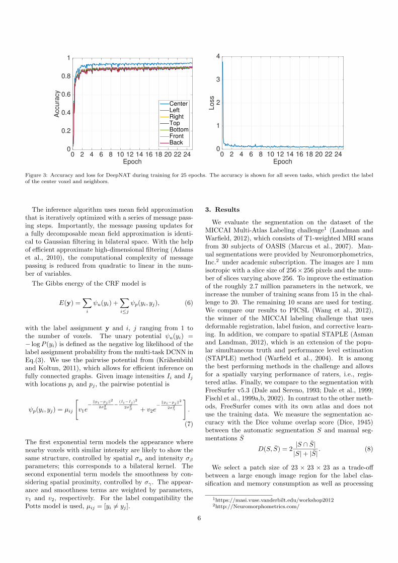
Figure 3: Accuracy and loss for DeepNAT during training for 25 epochs. The accuracy is shown for all seven tasks, which predict the labelof the center voxel and neighbors.

The inference algorithm uses mean field approximationthat is iteratively optimized with a series of message pass-ing steps. Importantly, the message passing updates fora fully decomposable mean field approximation is identi-cal to Gaussian filtering in bilateral space. With the helpof efficient approximate high-dimensional filtering (Adamset al., 2010), the computational complexity of messagepassing is reduced from quadratic to linear in the num-ber of variables.

The Gibbs energy of the CRF model is

E(y) =∑i

ψu(yi) +∑i≤j

ψp(yi, yj), (6)

with the label assignment y and i, j ranging from 1 tothe number of voxels. The unary potential ψu(yi) =− logP (yi) is defined as the negative log likelihood of thelabel assignment probability from the multi-task DCNN inEq.(3). We use the pairwise potential from (Krahenbuhland Koltun, 2011), which allows for efficient inference onfully connected graphs. Given image intensities Ii and Ijwith locations pi and pj , the pairwise potential is

ψp(yi, yj) = µij

[v1e−‖pi−pj‖

2

2σ2α−

(Ii−Ij)2

2σ2β + v2e

−‖pi−pj‖

2

2σ2γ

].

(7)

The first exponential term models the appearance wherenearby voxels with similar intensity are likely to show thesame structure, controlled by spatial σα and intensity σβparameters; this corresponds to a bilateral kernel. Thesecond exponential term models the smoothness by con-sidering spatial proximity, controlled by σγ . The appear-ance and smoothness terms are weighted by parameters,v1 and v2, respectively. For the label compatibility thePotts model is used, µij = [yi 6= yj ].

3. Results

We evaluate the segmentation on the dataset of theMICCAI Multi-Atlas Labeling challenge1 (Landman andWarfield, 2012), which consists of T1-weighted MRI scansfrom 30 subjects of OASIS (Marcus et al., 2007). Man-ual segmentations were provided by Neuromorphometrics,Inc.2 under academic subscription. The images are 1 mmisotropic with a slice size of 256× 256 pixels and the num-ber of slices varying above 256. To improve the estimationof the roughly 2.7 million parameters in the network, weincrease the number of training scans from 15 in the chal-lenge to 20. The remaining 10 scans are used for testing.We compare our results to PICSL (Wang et al., 2012),the winner of the MICCAI labeling challenge that usesdeformable registration, label fusion, and corrective learn-ing. In addition, we compare to spatial STAPLE (Asmanand Landman, 2012), which is an extension of the popu-lar simultaneous truth and performance level estimation(STAPLE) method (Warfield et al., 2004). It is amongthe best performing methods in the challenge and allowsfor a spatially varying performance of raters, i.e., regis-tered atlas. Finally, we compare to the segmentation withFreeSurfer v5.3 (Dale and Sereno, 1993; Dale et al., 1999;Fischl et al., 1999a,b, 2002). In contrast to the other meth-ods, FreeSurfer comes with its own atlas and does notuse the training data. We measure the segmentation ac-curacy with the Dice volume overlap score (Dice, 1945)between the automatic segmentation S and manual seg-mentations S

D(S, S) = 2|S ∩ S||S|+ |S|

. (8)

We select a patch size of 23 × 23 × 23 as a trade-offbetween a large enough image region for the label clas-sification and memory consumption as well as processing

1https://masi.vuse.vanderbilt.edu/workshop20122http://Neuromorphometrics.com/

6

DeepN

AT

Only

Spect

ral

Only

Cart

esi

an

No C

oord

inate

s

One S

tep

27

Task

s

1 T

ask

0.5

0.6

0.7

0.8

0.9

1.0

Method Median Dice

DeepNAT 0.897

Only Spectral 0.895Only Cartesian 0.892No Coordinates 0.878

One Step 0.879

27 Tasks 0.8851 Task 0.820

Figure 4: Segmentation results in Dice for different configurationsof DeepNAT. In the figure, red line indicates the median, the boxesextend to the 25th and 75th percentiles, and the whiskers reach tothe most extreme values not considered outliers (crosses). The tablelists the median Dice for the different variations in the DeepNATconfiguration.

speed. DeepNAT is based on the Caffe framework (Jiaet al., 2014). Gradients are computed on minibatches,where each gradient update is the average of the individ-ual gradients of the patches in the minibatch. The size ofthe minibatch is constrained by the memory of the GPU,where a size of 2,048 fills up most of the 12GB GPU mem-ory on the NVIDIA Tesla K40 and TITAN X used in theexperiments. Large batch sizes are advisable as they bet-ter approximate the true gradient.

We train the network with stochastic gradient descentand the “poly” scheme (also applied by Chen et al. (2016))using a base learning rate of 0.01. The actual learningrate at each iteration is the base learning rate multipliedby (1− iteration/max iteration)0.9, promoting larger stepsat the beginning of the training period and smaller stepstowards the end. For the first network, we randomly sam-ple 30,000 patches from the foreground and background in

DeepN

AT

DeepN

ATcr

f

FreeSurf

er

Spati

al Sta

ple

PIC

SL0.5

0.6

0.7

0.8

0.9

1.0

Method Median Dice

DeepNAT 0.910DeepNATcrf 0.920FreeSurfer 0.819Spatial STAPLE 0.897PICSL 0.912

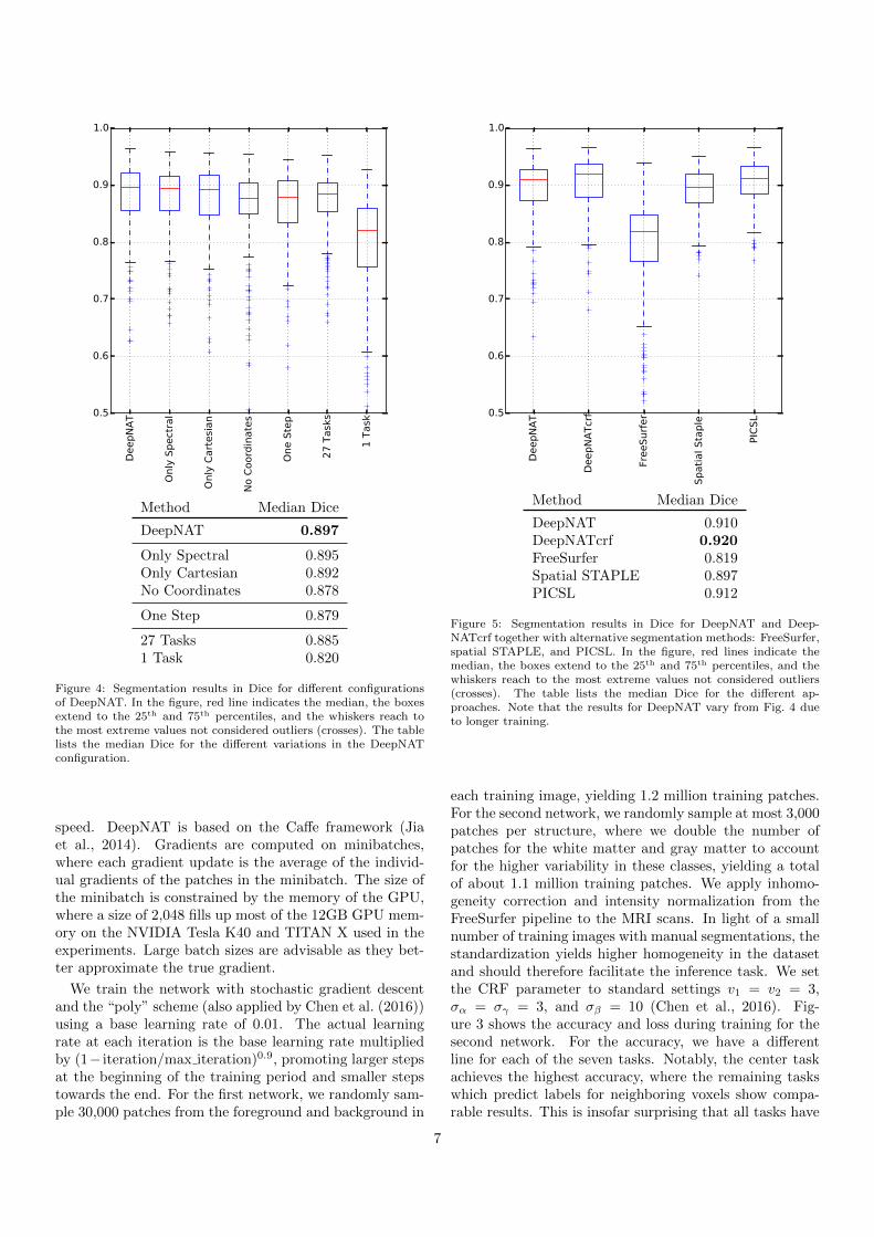
Figure 5: Segmentation results in Dice for DeepNAT and Deep-NATcrf together with alternative segmentation methods: FreeSurfer,spatial STAPLE, and PICSL. In the figure, red lines indicate themedian, the boxes extend to the 25th and 75th percentiles, and thewhiskers reach to the most extreme values not considered outliers(crosses). The table lists the median Dice for the different ap-proaches. Note that the results for DeepNAT vary from Fig. 4 dueto longer training.

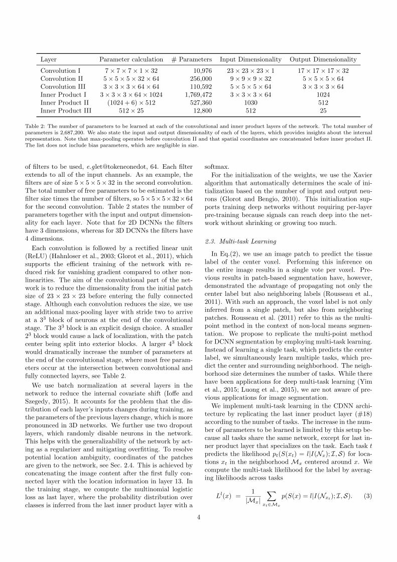
each training image, yielding 1.2 million training patches.For the second network, we randomly sample at most 3,000patches per structure, where we double the number ofpatches for the white matter and gray matter to accountfor the higher variability in these classes, yielding a totalof about 1.1 million training patches. We apply inhomo-geneity correction and intensity normalization from theFreeSurfer pipeline to the MRI scans. In light of a smallnumber of training images with manual segmentations, thestandardization yields higher homogeneity in the datasetand should therefore facilitate the inference task. We setthe CRF parameter to standard settings v1 = v2 = 3,σα = σγ = 3, and σβ = 10 (Chen et al., 2016). Fig-ure 3 shows the accuracy and loss during training for thesecond network. For the accuracy, we have a differentline for each of the seven tasks. Notably, the center taskachieves the highest accuracy, where the remaining taskswhich predict labels for neighboring voxels show compa-rable results. This is insofar surprising that all tasks have

7

DeepN

AT

DeepN

ATcr

f

FreeSurf

er

Spati

al Sta

ple

PIC

SL0.75

0.80

0.85

0.90

Dic

e

Method Mean Dice

DeepNAT 0.894DeepNATcrf 0.906FreeSurfer 0.790Spatial STAPLE 0.890PICSL 0.904

Figure 6: Segmentation results in Dice for DeepNAT and Deep-NATcrf together with alternative segmentation methods: FreeSurfer,spatial STAPLE, and PICSL. The bars show the mean Dice score andthe lines show the standard error. The table lists the mean Dice forthe different approaches.

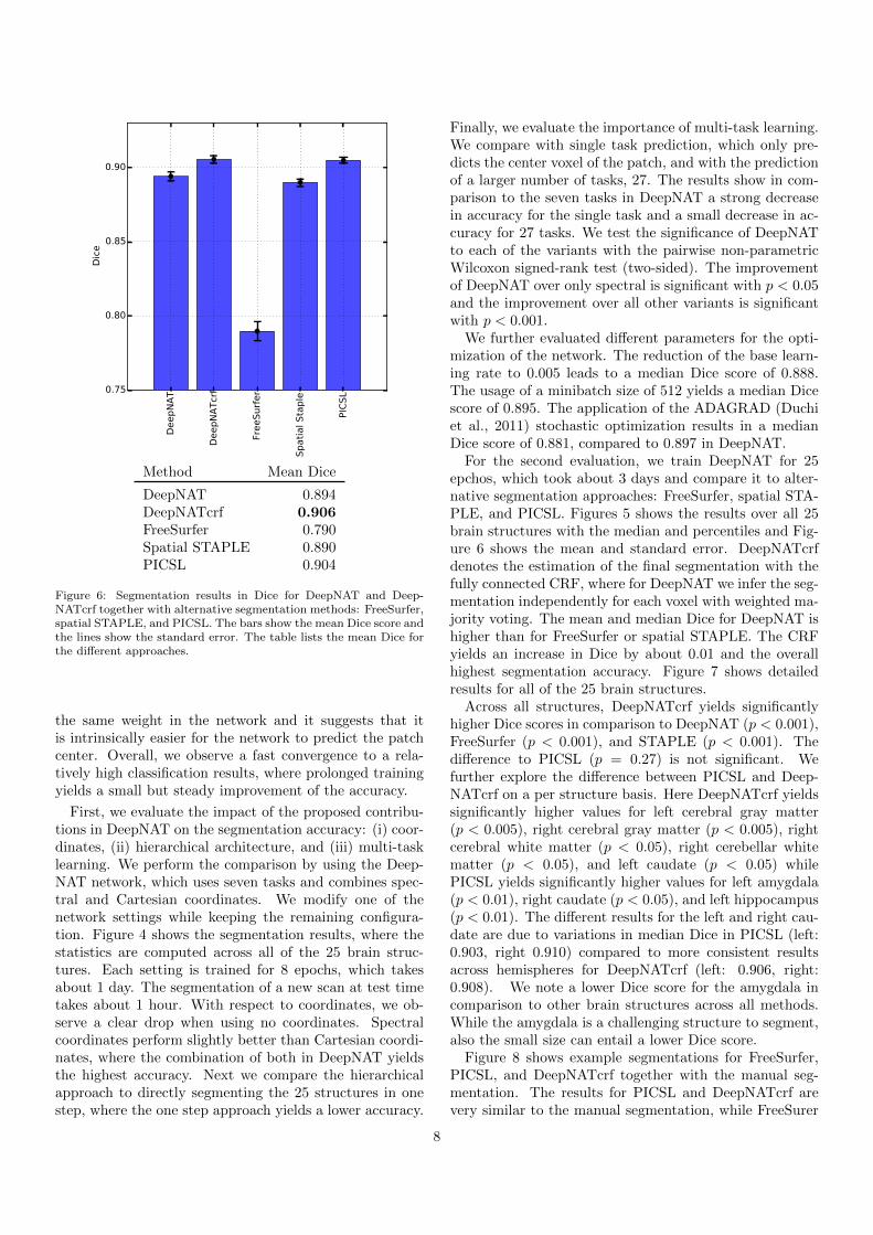
the same weight in the network and it suggests that itis intrinsically easier for the network to predict the patchcenter. Overall, we observe a fast convergence to a rela-tively high classification results, where prolonged trainingyields a small but steady improvement of the accuracy.

First, we evaluate the impact of the proposed contribu-tions in DeepNAT on the segmentation accuracy: (i) coor-dinates, (ii) hierarchical architecture, and (iii) multi-tasklearning. We perform the comparison by using the Deep-NAT network, which uses seven tasks and combines spec-tral and Cartesian coordinates. We modify one of thenetwork settings while keeping the remaining configura-tion. Figure 4 shows the segmentation results, where thestatistics are computed across all of the 25 brain struc-tures. Each setting is trained for 8 epochs, which takesabout 1 day. The segmentation of a new scan at test timetakes about 1 hour. With respect to coordinates, we ob-serve a clear drop when using no coordinates. Spectralcoordinates perform slightly better than Cartesian coordi-nates, where the combination of both in DeepNAT yieldsthe highest accuracy. Next we compare the hierarchicalapproach to directly segmenting the 25 structures in onestep, where the one step approach yields a lower accuracy.

Finally, we evaluate the importance of multi-task learning.We compare with single task prediction, which only pre-dicts the center voxel of the patch, and with the predictionof a larger number of tasks, 27. The results show in com-parison to the seven tasks in DeepNAT a strong decreasein accuracy for the single task and a small decrease in ac-curacy for 27 tasks. We test the significance of DeepNATto each of the variants with the pairwise non-parametricWilcoxon signed-rank test (two-sided). The improvementof DeepNAT over only spectral is significant with p < 0.05and the improvement over all other variants is significantwith p < 0.001.

We further evaluated different parameters for the opti-mization of the network. The reduction of the base learn-ing rate to 0.005 leads to a median Dice score of 0.888.The usage of a minibatch size of 512 yields a median Dicescore of 0.895. The application of the ADAGRAD (Duchiet al., 2011) stochastic optimization results in a medianDice score of 0.881, compared to 0.897 in DeepNAT.

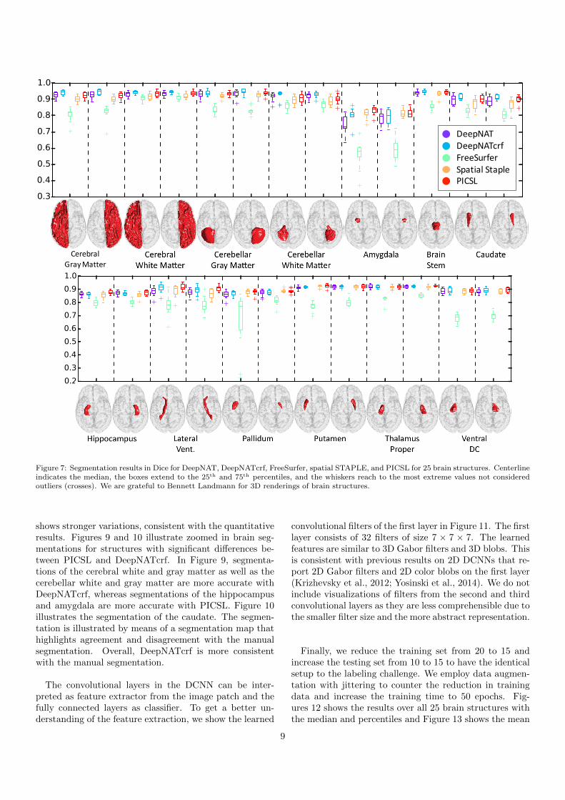
For the second evaluation, we train DeepNAT for 25epchos, which took about 3 days and compare it to alter-native segmentation approaches: FreeSurfer, spatial STA-PLE, and PICSL. Figures 5 shows the results over all 25brain structures with the median and percentiles and Fig-ure 6 shows the mean and standard error. DeepNATcrfdenotes the estimation of the final segmentation with thefully connected CRF, where for DeepNAT we infer the seg-mentation independently for each voxel with weighted ma-jority voting. The mean and median Dice for DeepNAT ishigher than for FreeSurfer or spatial STAPLE. The CRFyields an increase in Dice by about 0.01 and the overallhighest segmentation accuracy. Figure 7 shows detailedresults for all of the 25 brain structures.

Across all structures, DeepNATcrf yields significantlyhigher Dice scores in comparison to DeepNAT (p < 0.001),FreeSurfer (p < 0.001), and STAPLE (p < 0.001). Thedifference to PICSL (p = 0.27) is not significant. Wefurther explore the difference between PICSL and Deep-NATcrf on a per structure basis. Here DeepNATcrf yieldssignificantly higher values for left cerebral gray matter(p < 0.005), right cerebral gray matter (p < 0.005), rightcerebral white matter (p < 0.05), right cerebellar whitematter (p < 0.05), and left caudate (p < 0.05) whilePICSL yields significantly higher values for left amygdala(p < 0.01), right caudate (p < 0.05), and left hippocampus(p < 0.01). The different results for the left and right cau-date are due to variations in median Dice in PICSL (left:0.903, right 0.910) compared to more consistent resultsacross hemispheres for DeepNATcrf (left: 0.906, right:0.908). We note a lower Dice score for the amygdala incomparison to other brain structures across all methods.While the amygdala is a challenging structure to segment,also the small size can entail a lower Dice score.

Figure 8 shows example segmentations for FreeSurfer,PICSL, and DeepNATcrf together with the manual seg-mentation. The results for PICSL and DeepNATcrf arevery similar to the manual segmentation, while FreeSurer

8

0

0.2

0.4

0.6

0.8

1

0

0.2

0.4

0.6

0.8

1

0

0.2

0.4

0.6

0.8

1

0

0.2

0.4

0.6

0.8

1

CerebralGray  Matter

0

0.2

0.4

0.6

0.8

1

0

0.2

0.4

0.6

0.8

1

0

0.2

0.4

0.6

0.8

1

0

0.2

0.4

0.6

0.8

1

0

0.2

0.4

0.6

0.8

1

0

0.2

0.4

0.6

0.8

1

0

0.2

0.4

0.6

0.8

1

0

0.2

0.4

0.6

0.8

1

DeepNATDeepNATcrfFreeSurferSpatial  StaplePICSL  

Figure 7: Segmentation results in Dice for DeepNAT, DeepNATcrf, FreeSurfer, spatial STAPLE, and PICSL for 25 brain structures. Centerlineindicates the median, the boxes extend to the 25th and 75th percentiles, and the whiskers reach to the most extreme values not consideredoutliers (crosses). We are grateful to Bennett Landmann for 3D renderings of brain structures.

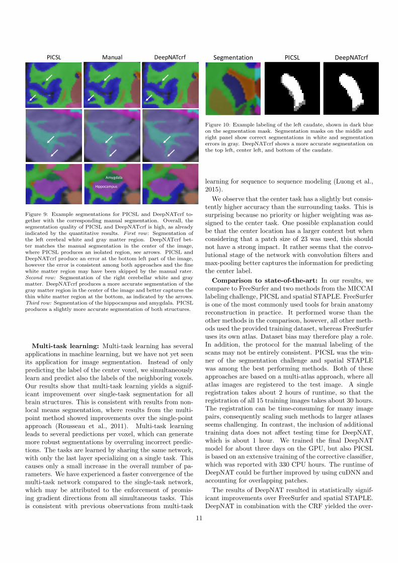
shows stronger variations, consistent with the quantitativeresults. Figures 9 and 10 illustrate zoomed in brain seg-mentations for structures with significant differences be-tween PICSL and DeepNATcrf. In Figure 9, segmenta-tions of the cerebral white and gray matter as well as thecerebellar white and gray matter are more accurate withDeepNATcrf, whereas segmentations of the hippocampusand amygdala are more accurate with PICSL. Figure 10illustrates the segmentation of the caudate. The segmen-tation is illustrated by means of a segmentation map thathighlights agreement and disagreement with the manualsegmentation. Overall, DeepNATcrf is more consistentwith the manual segmentation.

The convolutional layers in the DCNN can be inter-preted as feature extractor from the image patch and thefully connected layers as classifier. To get a better un-derstanding of the feature extraction, we show the learned

convolutional filters of the first layer in Figure 11. The firstlayer consists of 32 filters of size 7 × 7 × 7. The learnedfeatures are similar to 3D Gabor filters and 3D blobs. Thisis consistent with previous results on 2D DCNNs that re-port 2D Gabor filters and 2D color blobs on the first layer(Krizhevsky et al., 2012; Yosinski et al., 2014). We do notinclude visualizations of filters from the second and thirdconvolutional layers as they are less comprehensible due tothe smaller filter size and the more abstract representation.

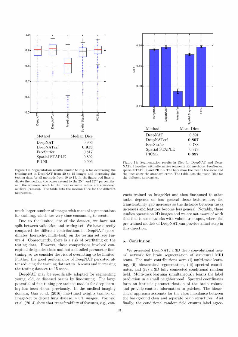
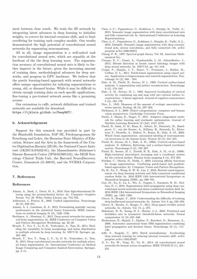
Finally, we reduce the training set from 20 to 15 andincrease the testing set from 10 to 15 to have the identicalsetup to the labeling challenge. We employ data augmen-tation with jittering to counter the reduction in trainingdata and increase the training time to 50 epochs. Fig-ures 12 shows the results over all 25 brain structures withthe median and percentiles and Figure 13 shows the mean

9

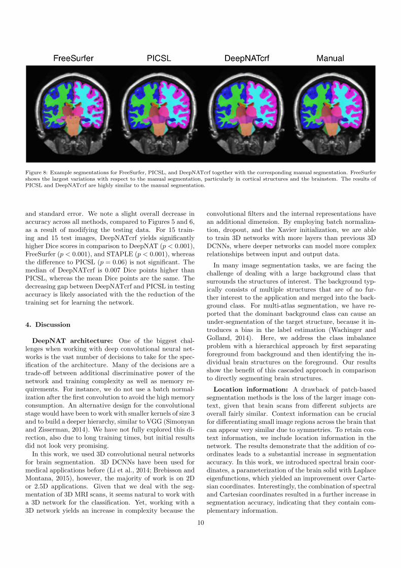
Figure 8: Example segmentations for FreeSurfer, PICSL, and DeepNATcrf together with the corresponding manual segmentation. FreeSurfershows the largest variations with respect to the manual segmentation, particularly in cortical structures and the brainstem. The results ofPICSL and DeepNATcrf are highly similar to the manual segmentation.

and standard error. We note a slight overall decrease inaccuracy across all methods, compared to Figures 5 and 6,as a result of modifying the testing data. For 15 train-ing and 15 test images, DeepNATcrf yields significantlyhigher Dice scores in comparison to DeepNAT (p < 0.001),FreeSurfer (p < 0.001), and STAPLE (p < 0.001), whereasthe difference to PICSL (p = 0.06) is not significant. Themedian of DeepNATcrf is 0.007 Dice points higher thanPICSL, whereas the mean Dice points are the same. Thedecreasing gap between DeepNATcrf and PICSL in testingaccuracy is likely associated with the the reduction of thetraining set for learning the network.

4. Discussion

DeepNAT architecture: One of the biggest chal-lenges when working with deep convolutional neural net-works is the vast number of decisions to take for the spec-ification of the architecture. Many of the decisions are atrade-off between additional discriminative power of thenetwork and training complexity as well as memory re-quirements. For instance, we do not use a batch normal-ization after the first convolution to avoid the high memoryconsumption. An alternative design for the convolutionalstage would have been to work with smaller kernels of size 3and to build a deeper hierarchy, similar to VGG (Simonyanand Zisserman, 2014). We have not fully explored this di-rection, also due to long training times, but initial resultsdid not look very promising.

In this work, we used 3D convolutional neural networksfor brain segmentation. 3D DCNNs have been used formedical applications before (Li et al., 2014; Brebisson andMontana, 2015), however, the majority of work is on 2Dor 2.5D applications. Given that we deal with the seg-mentation of 3D MRI scans, it seems natural to work witha 3D network for the classification. Yet, working with a3D network yields an increase in complexity because the

convolutional filters and the internal representations havean additional dimension. By employing batch normaliza-tion, dropout, and the Xavier initialization, we are ableto train 3D networks with more layers than previous 3DDCNNs, where deeper networks can model more complexrelationships between input and output data.

In many image segmentation tasks, we are facing thechallenge of dealing with a large background class thatsurrounds the structures of interest. The background typ-ically consists of multiple structures that are of no fur-ther interest to the application and merged into the back-ground class. For multi-atlas segmentation, we have re-ported that the dominant background class can cause anunder-segmentation of the target structure, because it in-troduces a bias in the label estimation (Wachinger andGolland, 2014). Here, we address the class imbalanceproblem with a hierarchical approach by first separatingforeground from background and then identifying the in-dividual brain structures on the foreground. Our resultsshow the benefit of this cascaded approach in comparisonto directly segmenting brain structures.

Location information: A drawback of patch-basedsegmentation methods is the loss of the larger image con-text, given that brain scans from different subjects areoverall fairly similar. Context information can be crucialfor differentiating small image regions across the brain thatcan appear very similar due to symmetries. To retain con-text information, we include location information in thenetwork. The results demonstrate that the addition of co-ordinates leads to a substantial increase in segmentationaccuracy. In this work, we introduced spectral brain coor-dinates, a parameterization of the brain solid with Laplaceeigenfunctions, which yielded an improvement over Carte-sian coordinates. Interestingly, the combination of spectraland Cartesian coordinates resulted in a further increase insegmentation accuracy, indicating that they contain com-plementary information.

10

DeepNATcrfPICSL Manual

Hippocampus

Amygdala

Figure 9: Example segmentations for PICSL and DeepNATcrf to-gether with the corresponding manual segmentation. Overall, thesegmentation quality of PICSL and DeepNATcrf is high, as alreadyindicated by the quantitative results. First row : Segmentation ofthe left cerebral white and gray matter region. DeepNATcrf bet-ter matches the manual segmentation in the center of the image,where PICSL produces an isolated region, see arrows. PICSL andDeepNATcrf produce an error at the bottom left part of the image,however the error is consistent among both approaches and the finewhite matter region may have been skipped by the manual rater.Second row: Segmentation of the right cerebellar white and graymatter. DeepNATcrf produces a more accurate segmentation of thegray matter region in the center of the image and better captures thethin white matter region at the bottom, as indicated by the arrows.Third row: Segmentation of the hippocampus and amygdala. PICSLproduces a slightly more accurate segmentation of both structures.

Multi-task learning: Multi-task learning has severalapplications in machine learning, but we have not yet seenits application for image segmentation. Instead of onlypredicting the label of the center voxel, we simultaneouslylearn and predict also the labels of the neighboring voxels.Our results show that multi-task learning yields a signif-icant improvement over single-task segmentation for allbrain structures. This is consistent with results from non-local means segmentation, where results from the multi-point method showed improvements over the single-pointapproach (Rousseau et al., 2011). Multi-task learningleads to several predictions per voxel, which can generatemore robust segmentations by overruling incorrect predic-tions. The tasks are learned by sharing the same network,with only the last layer specializing on a single task. Thiscauses only a small increase in the overall number of pa-rameters. We have experienced a faster convergence of themulti-task network compared to the single-task network,which may be attributed to the enforcement of promis-ing gradient directions from all simultaneous tasks. Thisis consistent with previous observations from multi-task

PICSLSegmentation DeepNATcrf

Figure 10: Example labeling of the left caudate, shown in dark blueon the segmentation mask. Segmentation masks on the middle andright panel show correct segmentations in white and segmentationerrors in gray. DeepNATcrf shows a more accurate segmentation onthe top left, center left, and bottom of the caudate.

learning for sequence to sequence modeling (Luong et al.,2015).

We observe that the center task has a slightly but consis-tently higher accuracy than the surrounding tasks. This issurprising because no priority or higher weighting was as-signed to the center task. One possible explanation couldbe that the center location has a larger context but whenconsidering that a patch size of 23 was used, this shouldnot have a strong impact. It rather seems that the convo-lutional stage of the network with convolution filters andmax-pooling better captures the information for predictingthe center label.

Comparison to state-of-the-art: In our results, wecompare to FreeSurfer and two methods from the MICCAIlabeling challenge, PICSL and spatial STAPLE. FreeSurferis one of the most commonly used tools for brain anatomyreconstruction in practice. It performed worse than theother methods in the comparison, however, all other meth-ods used the provided training dataset, whereas FreeSurferuses its own atlas. Dataset bias may therefore play a role.In addition, the protocol for the manual labeling of thescans may not be entirely consistent. PICSL was the win-ner of the segmentation challenge and spatial STAPLEwas among the best performing methods. Both of theseapproaches are based on a multi-atlas approach, where allatlas images are registered to the test image. A singleregistration takes about 2 hours of runtime, so that theregistration of all 15 training images takes about 30 hours.The registration can be time-consuming for many imagepairs, consequently scaling such methods to larger atlasesseems challenging. In contrast, the inclusion of additionaltraining data does not affect testing time for DeepNAT,which is about 1 hour. We trained the final DeepNATmodel for about three days on the GPU, but also PICSLis based on an extensive training of the corrective classifier,which was reported with 330 CPU hours. The runtime ofDeepNAT could be further improved by using cuDNN andaccounting for overlapping patches.

The results of DeepNAT resulted in statistically signif-icant improvements over FreeSurfer and spatial STAPLE.DeepNAT in combination with the CRF yielded the over-

11

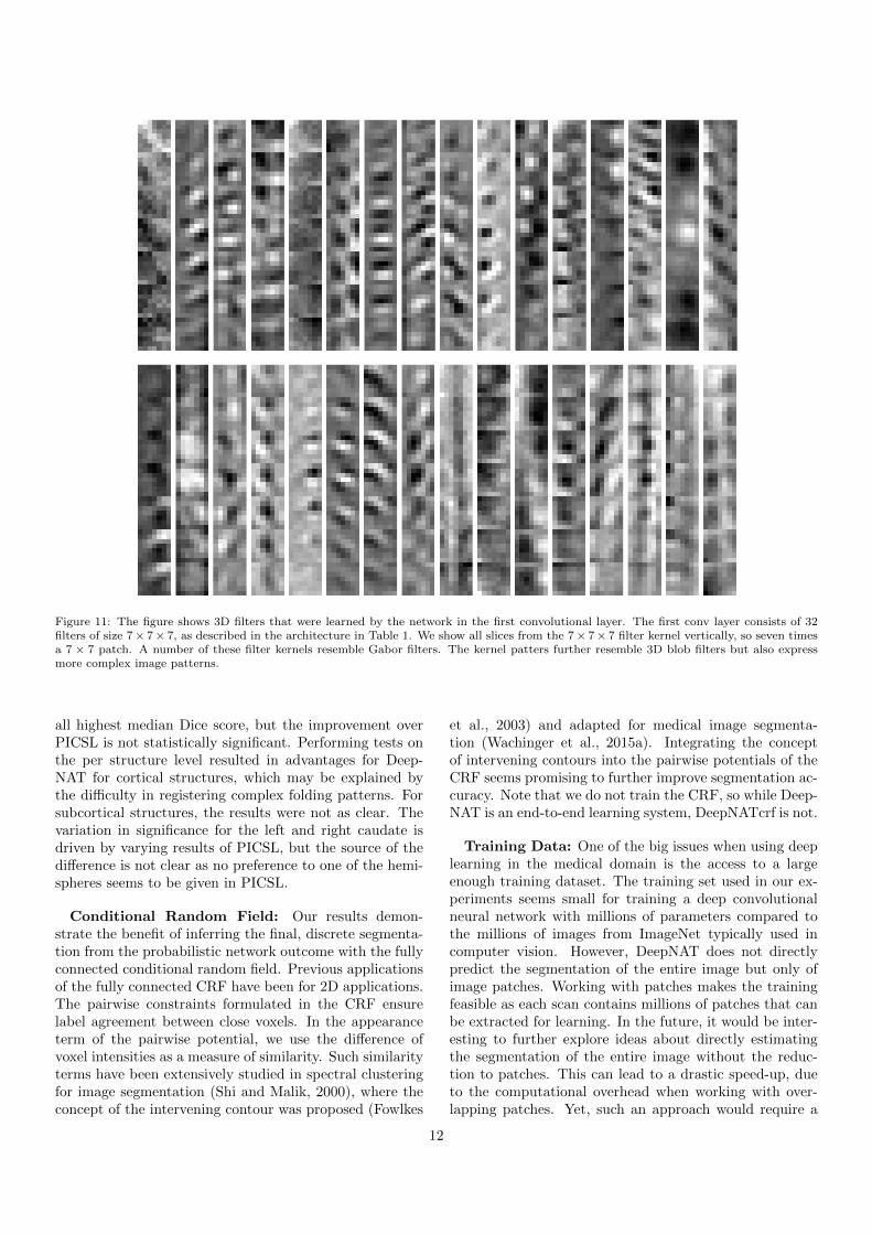
Figure 11: The figure shows 3D filters that were learned by the network in the first convolutional layer. The first conv layer consists of 32filters of size 7× 7× 7, as described in the architecture in Table 1. We show all slices from the 7× 7× 7 filter kernel vertically, so seven timesa 7 × 7 patch. A number of these filter kernels resemble Gabor filters. The kernel patters further resemble 3D blob filters but also expressmore complex image patterns.

all highest median Dice score, but the improvement overPICSL is not statistically significant. Performing tests onthe per structure level resulted in advantages for Deep-NAT for cortical structures, which may be explained bythe difficulty in registering complex folding patterns. Forsubcortical structures, the results were not as clear. Thevariation in significance for the left and right caudate isdriven by varying results of PICSL, but the source of thedifference is not clear as no preference to one of the hemi-spheres seems to be given in PICSL.

Conditional Random Field: Our results demon-strate the benefit of inferring the final, discrete segmenta-tion from the probabilistic network outcome with the fullyconnected conditional random field. Previous applicationsof the fully connected CRF have been for 2D applications.The pairwise constraints formulated in the CRF ensurelabel agreement between close voxels. In the appearanceterm of the pairwise potential, we use the difference ofvoxel intensities as a measure of similarity. Such similarityterms have been extensively studied in spectral clusteringfor image segmentation (Shi and Malik, 2000), where theconcept of the intervening contour was proposed (Fowlkes

et al., 2003) and adapted for medical image segmenta-tion (Wachinger et al., 2015a). Integrating the conceptof intervening contours into the pairwise potentials of theCRF seems promising to further improve segmentation ac-curacy. Note that we do not train the CRF, so while Deep-NAT is an end-to-end learning system, DeepNATcrf is not.

Training Data: One of the big issues when using deeplearning in the medical domain is the access to a largeenough training dataset. The training set used in our ex-periments seems small for training a deep convolutionalneural network with millions of parameters compared tothe millions of images from ImageNet typically used incomputer vision. However, DeepNAT does not directlypredict the segmentation of the entire image but only ofimage patches. Working with patches makes the trainingfeasible as each scan contains millions of patches that canbe extracted for learning. In the future, it would be inter-esting to further explore ideas about directly estimatingthe segmentation of the entire image without the reduc-tion to patches. This can lead to a drastic speed-up, dueto the computational overhead when working with over-lapping patches. Yet, such an approach would require a

12

DeepN

AT

DeepN

ATcr

f

FreeSurf

er

Spati

al Sta

ple

PIC

SL0.5

0.6

0.7

0.8

0.9

1.0

Method Median Dice

DeepNAT 0.906DeepNATcrf 0.913FreeSurfer 0.817Spatial STAPLE 0.892PICSL 0.906

Figure 12: Segmentation results similar to Fig. 5 for decreasing thetraining set in DeepNAT from 20 to 15 images and increasing thetesting data for all methods from 10 to 15. In the figure, red lines in-dicate the median, the boxes extend to the 25th and 75th percentiles,and the whiskers reach to the most extreme values not consideredoutliers (crosses). The table lists the median Dice for the differentapproaches.

much larger number of images with manual segmentationsfor training, which are very time consuming to create.

Due to the limited size of the dataset, we have notsplit between validation and testing set. We have directlycompared the different contributions in DeepNAT (coor-dinates, hierarchy, multi-task) on the testing set, see Fig-ure 4. Consequently, there is a risk of overfitting on thetesting data. However, these comparisons involved con-ceptual design decisions and not a detailed parameter fine-tuning, so we consider the risk of overfitting to be limited.Further, the good performance of DeepNAT persisted af-ter reducing the training dataset to 15 scans and increasingthe testing dataset to 15 scans.

DeepNAT may be specifically adapted for segmentingyoung, old, or diseased brains by fine-tuning. The largepotential of fine-tuning pre-trained models for deep learn-ing has been shown previously. In the medical imagingdomain, Gao et al. (2016) fine-tuned weights trained onImageNet to detect lung disease in CT images. Yosinskiet al. (2014) show that transferability of features, e.g., con-

DeepN

AT

DeepN

ATcr

f

FreeSurf

er

Spati

al Sta

ple

PIC

SL0.75

0.80

0.85

0.90

Dic

e

Method Mean Dice

DeepNAT 0.891DeepNATcrf 0.897FreeSurfer 0.788Spatial STAPLE 0.878PICSL 0.897

Figure 13: Segmentation results in Dice for DeepNAT and Deep-NATcrf together with alternative segmentation methods: FreeSurfer,spatial STAPLE, and PICSL. The bars show the mean Dice score andthe lines show the standard error. The table lists the mean Dice forthe different approaches.

vnets trained on ImageNet and then fine-tuned to othertasks, depends on how general those features are; thetransferability gap increases as the distance between tasksincreases and features become less general. Notably, thesestudies operate on 2D images and we are not aware of workthat fine-tunes networks with volumetric input, where thepre-trained models of DeepNAT can provide a first step inthis direction.

5. Conclusion

We presented DeepNAT, a 3D deep convolutional neu-ral network for brain segmentation of structural MRIscans. The main contributions were (i) multi-task learn-ing, (ii) hierarchical segmentation, (iii) spectral coordi-nates, and (iv) a 3D fully connected conditional randomfield. Multi-task learning simultaneously learns the labelprediction in a small neighborhood. Spectral coordinatesform an intrinsic parameterization of the brain volumeand provide context information to patches. The hierar-chical approach accounts for the class imbalance betweenthe background class and separate brain structures. Andfinally, the conditional random field ensures label agree-

13

ment between close voxels. We train the 3D network byintegrating latest advances in deep learning to initializeweights, to correct for internal covariate shift, and to limitoverfitting for training such complex models. Our resultsdemonstrated the high potential of convolutional neuralnetworks for segmenting neuroanatomy.

All in all, image segmentation is a well-suited taskfor convolutional neural nets, which are arguably at theforefront of the the deep learning wave. The segmenta-tion accuracy of convolutional neural nets is likely to fur-ther improve in the future, given the increasing amountof training data, methodological advances for deep net-works, and progress in GPU hardware. We believe thatthe purely learning-based approach with neural networksoffers unique opportunities for tailoring segmentations toyoung, old, or diseased brains. While it may be difficult toobtain enough training data on such specific applications,fine-tuning a pre-trained network seems like a promisingavenue.

Our extensions to caffe, network definitions and trainednetworks are available for download:https://tjklein.github.io/DeepNAT/.

6. Acknowledgement

Support for this research was provided in part bythe Humboldt foundation, SAP SE, Forderprogramm furForschung und Lehre, the Bavarian State Ministry of Edu-cation, Science and the Arts in the framework of the Cen-tre Digitisation.Bavaria (ZD.B), the National Cancer Insti-tute (1K25CA181632-01), the Massachusetts Alzheimer’sDisease Research Center (5P50AG005134), the MGH Neu-rology Clinical Trials Unit, the Harvard NeuroDiscoveryCenter, Genentech (G-40819), and the NVIDIA Corpora-tion.

7. References

References

Adams, A., Baek, J., Davis, M. A., 2010. Fast high-dimensional fil-tering using the permutohedral lattice. In: Computer GraphicsForum. Vol. 29. Wiley Online Library, pp. 753–762.

Ashburner, J., Friston, K., 2005. Unified segmentation. Neuroimage26 (3), 839–851.

Asman, A. J., Landman, B. A., 2012. Formulating spatially varyingperformance in the statistical fusion framework. IEEE transac-tions on medical imaging 31 (6), 1326–1336.

Brebisson, A., Montana, G., 2015. Deep neural networks for anatom-ical brain segmentation. In: IEEE Conference on Computer Visionand Pattern Recognition Workshops. pp. 20–28.

Brosch, T., Yoo, Y., Li, D. K., Traboulsee, A., Tam, R., 2014. Mod-eling the variability in brain morphology and lesion distributionin multiple sclerosis by deep learning. In: MICCAI. Springer, pp.462–469.

Brosch, T., Yoo, Y., Tang, L. Y., Li, D. K., Traboulsee, A., Tam,R., 2015. Deep convolutional encoder networks for multiple sclero-sis lesion segmentation. In: International Conference on MedicalImage Computing and Computer-Assisted Intervention. Springer,pp. 3–11.

Chen, L.-C., Papandreou, G., Kokkinos, I., Murphy, K., Yuille, A.,2015. Semantic image segmentation with deep convolutional netsand fully connected crfs. In: International Conference on LearningRepresentations.

Chen, L.-C., Papandreou, G., Kokkinos, I., Murphy, K., Yuille, A. L.,2016. Deeplab: Semantic image segmentation with deep convolu-tional nets, atrous convolution, and fully connected crfs. arXivpreprint arXiv:1606.00915.

Chung, F. R., 1997. Spectral graph theory. Vol. 92. American Math-ematical Soc.

Ciresan, D. C., Giusti, A., Gambardella, L. M., Schmidhuber, J.,2013. Mitosis detection in breast cancer histology images withdeep neural networks. In: MICCAI. pp. 411–418.

Coupe, P., Manjon, J. V., Fonov, V., Pruessner, J., Robles, M.,Collins, D. L., 2011. Patch-based segmentation using expert pri-ors: Application to hippocampus and ventricle segmentation. Neu-roImage 54 (2), 940 – 954.

Dale, A. M., Fischl, B., Sereno, M. I., 1999. Cortical surface-basedanalysis: I. segmentation and surface reconstruction. Neuroimage9 (2), 179–194.

Dale, A. M., Sereno, M. I., 1993. Improved localizadon of corticalactivity by combining eeg and meg with mri cortical surface re-construction: A linear approach. Journal of cognitive neuroscience5 (2), 162–176.

Dice, L., 1945. Measures of the amount of ecologic association be-tween species. Ecology 26 (3), 297–302.

Dickinson, S. J., 2009. Object categorization: computer and humanvision perspectives. Cambridge University Press.

Duchi, J., Hazan, E., Singer, Y., 2011. Adaptive subgradient meth-ods for online learning and stochastic optimization. Journal ofMachine Learning Research 12 (Jul), 2121–2159.

Fischl, B., Salat, D. H., Busa, E., Albert, M., Dieterich, M., Hasel-grove, C., van der Kouwe, A., Killiany, R., Kennedy, D., Klave-ness, S., Montillo, A., Makris, N., Rosen, B., Dale, A. M., 2002.Whole brain segmentation: automated labeling of neuroanatomi-cal structures in the human brain. Neuron 33 (3), 341–355.

Fischl, B., Sereno, M. I., Dale, A. M., 1999a. Cortical surface-basedanalysis: Ii: Inflation, flattening, and a surface-based coordinatesystem. Neuroimage 9 (2), 195–207.

Fischl, B., Sereno, M. I., Tootell, R. B., Dale, A. M., et al., 1999b.High-resolution intersubject averaging and a coordinate systemfor the cortical surface. Human brain mapping 8 (4), 272–284.

Fowlkes, C., Martin, D., Malik, J., 2003. Learning affinity functionsfor image segmentation: Combining patch-based and gradient-based approaches. In: Computer Vision and Pattern Recognition.

Fu, H., Xu, Y., Wong, D. W. K., Liu, J., 2016. Retinal vessel segmen-tation via deep learning network and fully-connected conditionalrandom fields. In: 2016 IEEE 13th International Symposium onBiomedical Imaging (ISBI). pp. 698–701.

Gao, M., Xu, Z., Lu, L., Wu, A., Nogues, I., Summers, R. M., Mol-lura, D. J., 2016. Segmentation label propagation using deep con-volutional neural networks and dense conditional random field. In:2016 IEEE 13th International Symposium on Biomedical Imaging(ISBI). pp. 1265–1268.

Glorot, X., Bengio, Y., 2010. Understanding the difficulty of trainingdeep feedforward neural networks. In: Aistats. Vol. 9. pp. 249–256.

Glorot, X., Bordes, A., Bengio, Y., 2011. Deep sparse rectifier neuralnetworks. In: Aistats. Vol. 15. p. 275.

Hahnloser, R. H., Seung, H. S., Slotine, J.-J., 2003. Permitted andforbidden sets in symmetric threshold-linear networks. Neuralcomputation 15 (3), 621–638.

Heckemann, R., Hajnal, J., Aljabar, P., Rueckert, D., Hammers, A.,2006. Automatic anatomical brain MRI segmentation combininglabel propagation and decision fusion. NeuroImage 33 (1), 115–126.

Ioffe, S., Szegedy, C., 2015. Batch normalization: Acceleratingdeep network training by reducing internal covariate shift. arXivpreprint arXiv:1502.03167.

Ji, S., Xu, W., Yang, M., Yu, K., 2013. 3d convolutional neuralnetworks for human action recognition. IEEE TPAMI 35 (1), 221–231.

14

Jia, Y., Shelhamer, E., Donahue, J., Karayev, S., Long, J., Gir-shick, R., Guadarrama, S., Darrell, T., 2014. Caffe: Convo-lutional architecture for fast feature embedding. arXiv preprintarXiv:1408.5093.

Krahenbuhl, P., Koltun, V., 2011. Efficient inference in fully con-nected crfs with gaussian edge potentials. In: Advances in NeuralInformation Processing Systems. pp. 109–117.

Krizhevsky, A., Sutskever, I., Hinton, G. E., 2012. Imagenet classifi-cation with deep convolutional neural networks. In: Advances inneural information processing systems. pp. 1097–1105.

Landman, B., Warfield, S., 2012. Miccai 2012 workshop on multi-atlas labeling. In: Medical Image Computing and Computer As-sisted Intervention Conference (MICCAI) Grand Challenge.

LeCun, Y., Boser, B., Denker, J. S., Henderson, D., Howard, R. E.,Hubbard, W., Jackel, L. D., 1989. Backpropagation applied tohandwritten zip code recognition. Neural Comput. 1 (4), 541–551.

Li, R., Zhang, W., Suk, H.-I., Wang, L., Li, J., Shen, D., Ji, S.,2014. Deep learning based imaging data completion for improvedbrain disease diagnosis. In: International Conference on MedicalImage Computing and Computer-Assisted Intervention. Springer,pp. 305–312.

Lombaert, H., Grady, L., Polimeni, J. R., Cheriet, F., 2013a. Focusr:Feature oriented correspondence using spectral regularization–amethod for precise surface matching. Pattern Analysis and Ma-chine Intelligence, IEEE Transactions on 35 (9), 2143–2160.

Lombaert, H., Sporring, J., Siddiqi, K., 2013b. Diffeomorphic spec-tral matching of cortical surfaces. In: IPMI. Springer, pp. 376–389.

Luong, M.-T., Le, Q. V., Sutskever, I., Vinyals, O., Kaiser, L.,2015. Multi-task sequence to sequence learning. arXiv preprintarXiv:1511.06114.

Marcus, D. S., Wang, T. H., Parker, J., Csernansky, J. G., Mor-ris, J. C., Buckner, R. L., 2007. Open access series of imagingstudies (oasis): cross-sectional mri data in young, middle aged,nondemented, and demented older adults. Journal of cognitiveneuroscience 19 (9), 1498–1507.

Pereira, S., Pinto, A., Alves, V., Silva, C. A., 2015. Deep Convolu-tional Neural Networks for the Segmentation of Gliomas in Multi-sequence MRI. Springer International Publishing, pp. 131–143.

Pohl, K., Fisher, J., Grimson, W., Kikinis, R., Wells, W., 2006. ABayesian model for joint segmentation and registration. Neuroim-age 31 (1), 228–239.

Prasoon, A., Petersen, K., Igel, C., Lauze, F., Dam, E., Nielsen,M., 2013. Deep feature learning for knee cartilage segmentationusing a triplanar convolutional neural network. In: MICCAI. pp.246–253.

Rohlfing, T., Brandt, R., Menzel, R., Maurer, C., et al., 2004. Evalu-ation of atlas selection strategies for atlas-based image segmenta-tion with application to confocal microscopy images of bee brains.NeuroImage 21 (4), 1428–1442.

Rohlfing, T., Brandt, R., Menzel, R., Russakoff, D., Maurer, C.,2005. Quo vadis, atlas-based segmentation? Handbook of Biomed-ical Image Analysis, 435–486.

Roth, H. R., Lu, L., Seff, A., Cherry, K. M., Hoffman, J., Wang,S., Liu, J., Turkbey, E., Summers, R. M., 2014. A new 2.5 drepresentation for lymph node detection using random sets of deepconvolutional neural network observations. In: MICCAI. pp. 520–527.

Rousseau, F., Habas, P. A., Studholme, C., 2011. A supervised patch-based approach for human brain labeling. IEEE Trans. Med. Imag-ing 30 (10), 1852–1862.

Sabuncu, M., Yeo, B., Van Leemput, K., Fischl, B., Golland, P.,2010. A Generative Model for Image Segmentation Based on LabelFusion. TMI 29.

Shi, J., Malik, J., 2000. Normalized cuts and image segmentation.Pattern Analysis and Machine Intelligence, IEEE Transactions on22 (8), 888–905.

Simonyan, K., Zisserman, A., 2014. Very deep convolutionalnetworks for large-scale image recognition. arXiv preprintarXiv:1409.1556.

Svarer, C., Madsen, K., Hasselbalch, S. G., Pinborg, L. H., Haugbøl,S., Frøkjær, V. G., Holm, S., Paulson, O. B., Knudsen, G. M.,

2005. Mr-based automatic delineation of volumes of interest in hu-man brain pet images using probability maps. Neuroimage 24 (4),969–979.

Wachinger, C., Brennan, M., Sharp, G., Golland, P., 2014. On theimportance of location and features for patch-based segmentationof parotid glands. In: MICCAI Workshop on Image-Guided Adap-tive Radiation Therapy. Midas Journal.

Wachinger, C., Brennan, M., Sharp, G., Golland, P., 2016. Efficientdescriptor-based segmentation of parotid glands with non-localmeans. IEEE Transactions on Biomedical Engineering PP (99),1–1.

Wachinger, C., Fritscher, K., Sharp, G., Golland, P., 2015a. Contour-driven atlas-based segmentation. IEEE transactions on medicalimaging 34 (12), 2492–2505.

Wachinger, C., Golland, P., 2014. Atlas-based under-segmentation.In: Medical Image Computing and Computer-AssistedIntervention–MICCAI 2014. Springer, pp. 315–322.

Wachinger, C., Golland, P., Kremen, W., Fischl, B., Reuter, M.,2015b. Brainprint: A discriminative characterization of brain mor-phology. NeuroImage 109, 232 – 248.

Wang, C., Komodakis, N., Paragios, N., 2013a. Markov random fieldmodeling, inference & learning in computer vision & image under-standing: A survey. Computer Vision and Image Understanding117 (11), 1610–1627.

Wang, H., Avants, B., Yushkevich, P. A., 2012. A combined joint la-bel fusion and corrective learning approach. MICCAI 2012 GrandChallenge and Workshop on Multi-Atlas Labeling.

Wang, H., Suh, J. W., Das, S. R., Pluta, J. B., Craige, C., Yushke-vich, P. A., 2013b. Multi-atlas segmentation with joint label fu-sion. IEEE transactions on pattern analysis and machine intelli-gence 35 (3), 611–623.

Warfield, S. K., Zou, K. H., Wells, W. M., 2004. Simultaneous truthand performance level estimation (staple): an algorithm for thevalidation of image segmentation. IEEE transactions on medicalimaging 23 (7), 903–921.

Yim, J., Jung, H., Yoo, B., Choi, C., Park, D., Kim, J., 2015. Ro-tating your face using multi-task deep neural network. In: IEEECVPR. pp. 676–684.

Yosinski, J., Clune, J., Bengio, Y., Lipson, H., 2014. How transfer-able are features in deep neural networks? In: Advances in neuralinformation processing systems. pp. 3320–3328.

Zhang, W., Li, R., Deng, H., Wang, L., Lin, W., Ji, S., Shen,D., 2015. Deep convolutional neural networks for multi-modalityisointense infant brain image segmentation. NeuroImage 108, 214–224.

Zheng, Y., Liu, D., Georgescu, B., Nguyen, H., Comaniciu, D., 2015.3D deep learning for efficient and robust landmark detection involumetric data. In: MICCAI.

Zikic, D., Glocker, B., Criminisi, A., 2013. Atlas encoding by ran-domized forests for efficient label propagation. In: InternationalConference on Medical Image Computing and Computer-AssistedIntervention. Springer, pp. 66–73.

15