default prediction model for sme’s: evidence from uk ......enhance its accuracy of prediction, the...

International Journal of Business and Management; Vol. 10, No. 2; 2015 ISSN 1833-3850 E-ISSN 1833-8119

Published by Canadian Center of Science and Education

81

Default Prediction Model for SME’s: Evidence from UK Market Using Financial Ratios

Huijuan Lin1 1 Beijing Institute of Technology Zhuhai Campus, China

Correspondence: Huijuan Lin, Beijing Institute of Technology Zhuhai Campus, China. E-mail: [email protected] Received: November 6, 2014 Accepted: November 3, 2014 Online Published: January 20, 2015

doi:10.5539/ijbm.v10n2p81 URL: http://dx.doi.org/10.5539/ijbm.v10n2p81 Abstract The paper discusses bankruptcy prediction model in the UK during the two last decades. My study is provided to support that the Original Altman’s Z-score (1968) might not valid to predict bankruptcy since the business environment changed a lot. However, there are many firms go to bankrupt recently and there is a need to study and improve the bankruptcy predictive ability. And the result shows that Altman’s Z-score has little predictive ability in bankruptcy prediction. Then, I use the recent data to renew the Z-score model by changing the coefficient of original Z-score. After compared to the original Altman’s Z-score model, I found that the renewed Z-score model has been improve to a reasonable accuracy rate. In addition, I found that the variable (Sales/ total assets) has little contribution to distinguishing the bankrupt and non-bankrupt firms.

Keywords: SME, UK Market, Financial Ratios 1. Introduction, Background and Objectives 1.1 Introduction and Background

Since recent economic environment changed and especially after the financial crisis in 2008, many firms are faced financial distress or bankrupt recently. Thus, for the need of early warnings of impending financial distress and the prediction of corporate bankruptcy become increasingly important to analysts and stakeholders in UK since the effect of a company becoming insolvent or financially distressed often leads to adverse consequences for many stakeholders. Although the area has been subject to much academic and professional research over the last 50 years, this paper different from others because I try to increase the accuracy of prediction model by using the recent data to renew the original Z-score model. Firstly, this dissertation discuss the key literatures of the prediction models including Altman’s Z-score, Altman’s Z’’ model, Ohlson’s model and Taffler’s UK Z-score on how are the researchers selecting samples, how to select financial ratios as predictors, how to construct the models, how to extent the Z-score model, making the comparison between the multiple discriminant analysis and other prediction techniques. Also I am critical to the bankruptcy prediction models. Furthermore, I attempt to test whether the original z-score is accurate or not by using recent samples during the recent two decades, and if not, I would use the recent samples to update the coefficient of Z-score and test its accuracy. Then I make a comparison of the original Altman’s Z-score and the renewed Z-score updated by recent data. Moreover, to enhance its accuracy of prediction, the extra financial ratio might need to be analyzed because some variables might not reflect the true status of the firms. Finally, to enhance the accuracy of prediction, I would suggest that combining use the Z-score renewed by recent data and financial ratio analysis to predict firm’s financial distress within consumer goods industry in UK and aim to help the stakeholders including customers, suppliers, banks and other lenders, equity investors, employees, investors in distressed debt, borrower auditors, rating agencies and regulators. To predict the firm’s financial health accuracy in advance and they can take action to minimize the loss or avoid the financial distress for their purpose.

1.2 The Objectives

This dissertation aims to improve the accuracy of predicting business failure due to insolvent within consumer goods industry in UK. The main hypothesis of my dissertation is that, the Altman’s Z-score (1968) might not relevant to today’s business environment. With renewed the coefficient of Z-score by recent data, the predictive ability would be improved. I study the bankruptcy firms and the non-bankrupt firms and examine the predictive

www.ccsenet.org/ijbm International Journal of Business and Management Vol. 10, No. 2; 2015

82

ability of Altman’s Z-score using recent data because the model is about forty years old as it might not stable over time and not relevant to today’s economic climate. After that, I use the data set, which to test the original Z-score model, to test the accuracy of a renewed coefficient Z-score which is renewed by the recent data. Comparing the accuracy of predicting of Original Altman’s Z-score (1968) and the renewed Z-score model, the original Altman’s Z-score model (1968) has little predictive ability. If the financial distress of these troubled firms could have been predicted early enough, could they have possible been avoid or not? If then, to enhance it is accuracy, it might need to analyze the extra financial ratios since the variables of Z-score might not reflect the overview of the firms and also some variables are adjusted by the accounting methods.

2. An Overview of Insolvency in UK 2.1 Definition of Key Terms

To study the firms have failed, firstly, we must understand the concepts of corporate insolvency and financial distress in UK.

The definition of financial distress states:

“Financial Distress arises when a company is unable to meet its debts” (Mumford, 2003).

In other words, a firm has financial distress when the company cannot cover its immediate debts at some point of time. However, there are two probably results of financial distress. One might that firms with financial distress but received some help from other firms and finally, they are not going to bankrupt and without other financial problem. But, in this case, there is financial distress cost associate with financial distress. The other result might that firms with financial distress will go bankrupt. Thus, firms with financial distress might go to bankrupt in the future. According to Insolvency Act (1986), a firm will go bankrupt when the individual or the organization cannot pay its financial obligation as they promised or the company’s assets are less than its liabilities. In addition, in terms of bankrupt costs, there are two scenarios. If the type of company is corporation, then the company has to pay back all the debts even when no company assets left, which means a corporation has joint and several obligation to pay all the company’s debts. If the company is a limited company, then they just need to pay the debts by all the remaining assets.

2.2 The Users of This Prediction Model

Apart from analysts and researchers, there are many stakeholders who would be interested in the application of prediction models of financial distress. Similar to credit rating, the prediction model of financial distress is aim to evaluate a firm’s ability to repay the loan or liability and monitor the existing liability to avoid bad debts happen. However, unlike the credit rating, the users of prediction of financial distress model are not only the creditors but also a wider range of interested parties. Thus, to identify the users of this model will help to improve the model. For example, different users might set different appropriate cut-off points in the model with different purpose, and this will lead to different result of accuracy. In this sense, to know the motivation of the users is very important for the prediction model.

2.2.1 Regulatory Authorities

According to Anthony Paul Wood (2009)，regulatory bodies have the responsibility for oversee the solvency and stability of certain industries. For example if the financial crisis happened will have impact on the whole society. For example the financial crisis happen in 2008, many financial institutions go bankrupt and this did not only have effect on the financial institutions but also relative to citizens life and security of the society, regulatory authorities would like to oversee the stability of certain industries by using prediction models.

2.2.2 Management

Insolvency to a firm will raise both direct and indirect costs. Direct costs include fees to professionals such as administration fee, lawyers. Indirect costs include the lost sales or profits that could be reduced by arranged earlier. Altman (1984b) estimated that “bankruptcy costs ranged from 11% to 17% of firm value up to three years prior to bankruptcy” (P172). Thus, if firms have an early warning of bankruptcy, they might have further strategies such as management arranging a merger with another firms or other plan.

2.2.3 Government Officials

Government Officials can use financial distress model to forecast the financial status of some industry and make the decision of how to the budget or grant to some industry. Also, forecasting the financial status of industries can help them to establish and adjust the policy of the industries or even the country. Moreover, they can use the financial distress prediction model to predict other country’s financial status, economics and help decide how to take the further step in the strategies.


83

2.2.4 Investors

The existing investors can use financial distress model to forecast the finance status of the firms to determine what they should do in the further step. Also, in the market, investors may use financial distress prediction model to adjust their investment strategies. Variables from financial statement during three to five years before bankruptcy, the financial ratios of failed firms start to behave different from those of non-failed firms. Aharony, Jones, and Swary (1980) compared the risk adjusted returns of forty-five industrial US companies that went bankrupt in the 1970-1978 and a group of sixty-five control firms which are matched in the same industry, similar firm size, roughly the same time with bankrupt firms, and daily rates of return were available. The average weekly risk-adjusted return for each group was calculated up to 312 weeks before firms failed.

Aharony, Jones, and Swary (1980) also indicates that the market is not reflected all publicly available information in stock price and indicates that approaching to bankrupt, the share price become abnormal during four years before bankrupt, especially 7 weeks before bankrupt, there is a sharp drop in the return difference. However, in this scenario, investors use the financial distress prediction model to obtain more information regarding the firms that may not fully reflected in its existing security price, so investors may be able to gain. Also, the potential investors such as private equity will be concern that the firms are financial distressed or not, since they will invest firms on the fair time to buy-in with the lowest price to maximum the profit.

2.2.5 Auditors

The auditors can use the financial distress prediction model to forecast whether the firm will go bankrupt or not in the next year and give the judgment that the firm going concern or not before they auditing the firm. This judgment will affect the asset and liability valuation methods that are deemed appropriate for financial statement.

3. Literature Review Bankruptcy prediction model on firms has been investigated well in the United State with published papers during the late 1960s to 1980s. In light of theoretical, literatures concerned with industrial enterprises generally including Beaver, W. (1966), Altman (1968), Deakin (1972, 1977), Altman et al. (1977), Ohlson (1980). And most of the prediction models in the bankruptcy prediction area are financial ratio based models. Thus, I only pick up some main literatures to discuss. I will discuss how the Beaver select samples since Altman and others researcher after Beaver are used Beaver’s method to select samples. Also, I will summarize how the Beaver use financial ratio as predictor to predict bankruptcy. Moreover, I will summarize what the Altman do to construct Z-score model and how to extent Z-score model into wider application. Later on, there are many models using other techniques rather than multiple discriminant analysis to predict bankruptcy, so I make a comparison about these models with multiple discriminant analysis to find out that multiple discriminant analysis is more appropriate.

3.1 Univariate Analysis

Early studies (FitPatrick, 1932; Merwin, 1942) of financial ratios provided evidence that there were some differences between the ratios of bankrupt firms and the ratios of non-bankrupt firms. Such as Smith and Winakor (1935) observed some differences between the ratios of bankrupt firms and non-bankrupt firms. They found that the mean of the various ratios (such as cash flow/ total debt, net income/ total asset, working capital/ total assets etc.) of the bankrupt firms up to ten years before bankrupt, are higher than those of the non-bankrupt firms. Although these findings gave the hints of the prediction of bankrupt and non-bankrupt firm, how to classify the bankrupt and non-bankrupt firms, what is the particular point to classify and also how accuracy of the classification still not know from these findings.

With these questions, one of the most influent working of predicting financial distress is the univariate ratio analysis found by Beaver. Beaver attempt to find out the usefulness of the differences of financial ratio sets in the prediction of failure and regard this purpose as the starting point for the usefulness of ratio analysis. In a real sense, his univariate analysis of several variables (financial ratios) offered some solutions of how to classify the bankrupt groups and non-bankrupt groups, what financial ratios can be a predictor to classify the groups and the most important is he gave a good example on how to select sample. Since the findings of Beaver give great hints on how to form the bankruptcy prediction models, I will discuss it in more detail.

3.1.1 Beaver How to Select Samples

Beaver collected financial ratios from seventy nine failed firms and a matching sample of non-failed firms chosen based on the same industry and the similar firm size over an eleven years period of time (1954 to 1964 inclusive) as observations. The method of selecting sample has been adopted by many researchers (such as Altman, Taffler) and I use this method to selecting sample in the empirical study as well regarding to the


84

appropriateness of this method. Considering different industry might have its own average value of financial ratio. For example, on average, the firms from financial institutions will have higher debt ratio than firms from other industries due to many assets and liabilities of financial institutions are evaluated by market value. Thus, the same industry of firms is important, when choosing the matching non-bankrupt firms. In terms of firm size of the matching firms, Beaver (1966) believe relationship between ratios and failure will change by different firm size. Also, Alexander (1949) showed that the statistical evidence of the time supports the idea that even if two firms have the same ratios, if one firm is larger than the other then that company will have less chance of failure than the smaller one. Thus, similar firm size is important when selecting samples. Finally, since it is easy to attain data from public using Moody’s Industrial Manual, Beaver select samples from public firms with similar firm size in the same industry.

3.1.2 Beaver How to Select Predictors

Beaver analysed each ratio separately and selected the most appropriated cut-off point so that the number of accurate classifications was maximized for that particular purpose. Beaver classified thirty ratios he selected into six groups and each group have similar or common characteristics. Also one ratio from each group was selected for further analysis since some were mere transformations of others and many shared common information so only one from each group was selected. The six ratios were selected so that each ratio provided as much additional information as possible, and provided the best results in mean. Those six ratios representing each group individually were: working capital to total assets, cash-flow to total debt, net income to total assets, the current ratio, total debt to total assets and the no credit interval. In the real sense, Beaver classify the ratio into different groups since each ratio carry its information varies with other ratios from the firm to avoid repeatedly reflect the same information used many ratios, which is the sense of classification. Furthermore, in order to distinguish the bankrupt group and non-bankrupt group, the mean differences between the bankrupt and non-bankrupt samples should be observed. After analysed the means of each ratio up to five years before bankruptcy, Beaver was able to confirm these expectation that some ratios have different means between the two samples of failed and non-failed firms. The mean value of Cash-flow to total debt, net income to total assets, working capital to total assets, current ratio and no credit interval in non-failed firms respectively is higher than that in failed firms, while mean value of total debt to total assets in non-failed firm is lower than that in failed firms. So Beaver found that, predictors such as Cash-flow to total debt, Net income to total assets, Total debt to total assets, Working capital to total assets, Current ratio and No credit interval representing different ability of the firms in terms of liabilities, assets, liquidity of cash flow and credit can be useful to distinguish the bankrupt firms and non-bankrupt firms. (Beaver, 1966).

Beaver’s studies gave hints on the Altman’s study. For example, Beaver classify the thirty ratios into six groups, but the Altman select financial ratios from five distinct categories. However, how to determine a point to divide the sample into two groups and after these two groups are being classify correctly still be a question.

In addition, Beaver isolated samples from bankrupt firms and non-bankrupt firms respectively for analysis and investigate the financial ratios from these two samples up to five years before bankrupt. His analysis assesses original samples using classification analysis. Then the model tested on a sample of firms other than the original one, which is a period after the original data source. After tested fourteen financial ratios, Beaver found that the cash flow to total debt ratio was the best predictor of classifying bankruptcy. Other important financial ratios were the debt to total assets and net income to total assets ratio, and the ‘no credit interval’. Beaver (1966).

In Beaver (1966) analysis, he studied that the best predictor (cash flow to total debt) showed an increasing overlap area in the samples when making comparison during the time period. In other words, even the best predictor (cash flow to total debt), the predictive ability of it will shift overtime. According to Beaver (1966), while the appropriate cut-off point was placed, using data up to one year before bankrupt, there is 87% predictive ability and drop to only 78% when using data up to five years before bankrupt, indicating that the further back in time you go, it is harder of the indicator to classify between bankrupt and non-bankrupt firms. However, there are many factors influence the result such as life-cycle of the firm, the environment during that time period and management strategies and so forth.

Even only the highest accuracy rate is 87% one year before bankrupt in Beaver’s model, Beaver suggests that the accuracy of predictive ability of the model may be overstated. There are many factor should be consider but the main reasons illustrated as follow. One is that some inter co-relationship between the financial ratios might influence the predictive ability, thereby Beaver suggests that using financial ratio to predict bankrupt and non-bankrupt should with caution. Also he suggested that perhaps it is better to use multivariate approaches which using a combination of several financial ratios and their adjustment instead of his univariate method to


85

predict bankrupt and non-bankrupt firms since difference variables can lead to different predictions even about the same firm.

3.2 The Altman Z-Score Model (1968)

After the research of Beaver (1966), to solve the problems of univariate model, Edward Altman contributed to the development of probably the most popularity bankruptcy prediction model, Original Altman’s Z-score, was use the statistic technique known as multiple discriminant analysis to the business failure classification. Moreover, multiple discriminant analysis is the methodology I will use in empirical study of this dissertation thereby I will give more detail about how it work. multiple discriminant analysis is a statistical technique which classifieds observations into particular groups, thereby in this case there are two groups, bankrupt firms and non-bankrupt firms.

3.2.1 Altman How to Select Samples

Altman (1968) used the sample method to collect samples but Altman focus on the Manufacturing industry only. The sample size of Altman’s study is thirty three firms each for bankrupt group and non-bankrupt group during the twenty year period 1946–1965. Samples are chosen based on similar firm size and the same industry and samples are not chosen from private companies since it is hard to attain the financial statement of bankrupt firms.

3.2.2 Altman How to Construct Z-Score Model

In terms of variable selections, similar with Beaver’s classification sense, Altman (1968) obtained twenty two potential variables from five distinct categories, which are liquidity, profitability, leverage, solvency and activity respectively, as significant predictors of financial distress. Altman (1968) suggested that the best univariate predictor, cash-flow to total debt, was not appropriate variable since it is lack of consistent appearance of precise depreciation data. According to Agresti, A. (1996), multiple discriminant analysis is used to establish a linear combination of the independent variables (different financial ratios of the data) which best classify between the groups; While distinguishing the groups, the multiple discriminant consider each individual ratio basis and also each ratio’s interaction with each other can be observed.

After running the multiple discriminant analysis repeatedly with different combinations of these ratios, according to individual contributions, inter-correlations, the predictive ability of each combination and judgement of analyst, the discriminant function was obtained as being the best discriminator between the bankrupt and non-bankrupt firms in manufacturing.

The Z-score model is expressed as follows:

Z = 1.2 + 1.4 +3.3 +0.6 +0.999

Where

= (current assets -current liabilities)/total assets,

= retained earnings/totals assets,

=earnings before interest and taxes/total assets,

= market value of preferred and common equity (number of shares x price of stock)/total liabilities,

= sales/total assets.

To place an appropriate cut-off point for classification, Altman (1968) determined the following cut-off point for Original Z-score model which has accompanies the model ever since. The implication of this formula is that while firms having Z-score above 2.99 classify into non-bankrupt groups and the greater the score, the greater the chance that the firm will not failed, those firms with score below 1.81 are classified into the bankrupt group. A grey area lies between the two values and in this area there is high probability of misclassification occurred. And the result shows that there is 95.5% accuracy of this prediction model when using the same sample as the one derived the predictive model and its coefficients. However, the true predictive ability is assessed reasonable when the model is applied to a hold-out sample. To test the predictive ability of his model further, Altman (1968) applied it to a hold-out samples and test model for failed firm and non-failed firm respectively. From twenty-five failed firms whose have similar firm size and in the same industry as the sample used to obtain this model and its coefficients, twenty four were classified into failed group, thus 96% is correctly identified by the model. For the sample of non-bankrupt firms, the overall sample is sixty-six. While fourteen are correctly classify into non-failed firms, ten firms lay in the gray area. Thus, the accuracy of this model in non-failed firms is 64%. In addition, Altman (1968) test the model again used the same sample in the second, third, fourth and fifth years prior to failure and Altman (1968) concluded that the Z-score has little predictive ability when the time is more


86

than two years. Thus, in my empirical study, I observed samples one year before they failed since the highest accuracy rate of Z-score model is one year before firms failed. Moreover, it indicates that the prediction ability of bankrupt firms is higher than that of non-bankrupt firms and this finding should be considered when using the Z-score model to forecast bankruptcy.

3.3 The Extension of Z-Score Model

After the developed of Z-score, Altman has extent his model into wider application. Regarding time stress, I only summarize two main relevant predictive models in my dissertation.

3.3.1 Z-Score Model Extent to Both Public and Private Companies

Altman (1983) revise the Z-score by including private companies in the prediction model. Also in this model, the variable market value of equity was completely replaced by the book value of equity.

Since the market value of private firm is not reliable, Altman change the market value into book value. The coefficients of earnings before interest and taxes/total assets and book value of equity/total liabilities have significant changed to 3.107 and 0.420 respectively while the other variables have slightly changed. Although the grey area has extended, the accuracy of predictive ability still drop to 91% by adding the private companies into observations. In other words, there is not good at predicting since the grey area can express as the overlapping area which cannot distinguish the bankrupt firms and non-bankrupt firms clearly. Thus, the Z-score model has better accuracy rate while without private companies in the sample.

3.3.2 Z-Score Model Extent to All Industries (Exclusive Financial Institutions)

Since the Z-score confine to a specific industry, Altman (1983) was attempt to provide a more general application for all industries (exclusive the financial institutions). Also he believe the sales/ total assets variable is particularly industry-sensitive, so he removes it in Z’’ model. And he found that the accuracy of Z’’ model is the same as Z’ model which is 91%.

In this circumstance, the highest accuracy of Altman’s prediction model is the original Z-score model, which is confine into a particular industry probably and might due to the characteristics of industries are different.

3.4 Other Prediction Models Not Using Multiple Discriminant Analysis

After the work of Altman (1968) and Beaver (1966), there are many prediction models using other techniques to predict bankruptcy. The Wilcox (1976) others researchers develop models using other techniques rather than using multiple discriminant analysis such as Wilcox (1976) use the gambling ruin game theory and others such as Hazard model, genetic algorithms, neural networks. Marais et al.(1984) applied Decision Trees such as Id3, C4.5 and Random Trees; Tam and Kiang(1992) applied Multilayer Perception (MLP), a neural network model and K-Nearest Neighbours (KNN); Fan and Palaniswami (2000) used Support Vector Machine (SVM) and Sarkar and Sriram (2001) applied Naive Bayes (NB). Techniques of ensembles, such as Boosting or Bagging, have been applied by Foster and Stine (2004), who combined C4.5 and Boosting; while Mukkamala et al. (2006) combined Bagging and Random Tree (BRT). During the 1980’s, logistic analysis (Ohlson’s O-score model) are found by Ohlson (1980) to estimate the probability of bankruptcy in a static model. More recently, during the 1990’s, many researchers (Serrano-Cinca, 1993; Back et al., 1994) produced the artificial neural networks. Moreover, Serrano-Cinca and du Jardin and Séverin(2011) applied Self Organizing Feature Maps in predicting bankruptcies while Olson et al. (2012) for a recent comparative analysis on data mining methods for bankruptcy prediction.

3.5 The Z-Score Model in the UK

Geographically, I analyze the Z-score model in UK in this dissertation thereby I summarize a significant prediction models applied in UK. Taffler and Tisshaw (1977) applied the multiple discriminant analysis to predicting failure in UK with forty-six firms each for failed and non-failed firms in manufacturing which are have similar size from 1968 to 1976. After observed 80 different ratios, Taffler and Tisshaw (1977) just use four ratios as variable in predictive function which is Profit before tax/current liabilities, Current assets/total liabilities, Current liabilities/total assets and No-credit interval. And the highest accuracy rate of this model was 97% one year before bankrupt. After the researches of Tisshaw & Taffler (1977), Taffler (1982), Taffler (1983), the finalized model was available in Taffler (2005) constructed a prediction model and the model has almost 98% accuracy of predictive ability in hold-out tests in manufacturing. The cut-off point for this model is zero, when Z-score of a firm lower than zero, it was belong to a group of failed firms. However, the accuracy of this model when applied in other industries (oil& gas, health care, consumer services etc.) will need a further study. Although T&T constructed a bankruptcy prediction model with high accuracy rate in UK, I still want to


87

construct a prediction model in good consumer industry in UK and hope to have the same accuracy rate.

3.6 Critics of the Z-Score Approach

First of all, Taffler (1995) argues that the Z-score model is good at ex-post forecasting but poor at ex-ante predicting. Secondly, the prediction model cannot forecast when the firm will go bankrupt since there are lots of factors can make the firm go to bankrupt besides financial distress. Thirdly, since in some particular industries (software), using market value to evaluate assets and liabilities in the financial statement, it is not appropriate that the Z-score model ignore the effect from market by based on accounting data. Finally, argument will concentrate on predictive ability of the Z-score model over time. Although Heine (2000) provided evidence that the model was robust over the thirty year period of 1968–1999 by showing the M1 accuracy of the Z-score model was 82%(1969–1975), 85%(1976–1995), and 94% (1997–1999) using the cut-off point 2.67 and data from one year priority to bankrupt, the accuracy was not high as the original samples. My hypothesis in the dissertation is that the original Altman’s Z-score prediction model does not valid today and this is tested in empirical study of this dissertation. In addition, the important part of my dissertation is that using the recent data to renew the coefficient of Z-score model by using discriminant analysis.

4. An Empirical Study This part of dissertation examines empirically the hypothesis that the use of original Altman’s Z-score model is out of date and is not relevant to the recent economic period. When applied the original Z-score model to the recent data, if the accuracy is low, it indicates that the Z-score model has little predictive ability to recent business. Using multiple discriminant analysis and data collection from recent UK public firms insolvency during the period 31 December 1988 to 31 December 2007 inclusive as observation, a new Z-score function model is developed to improve the accuracy of the Z-score prediction model. Then, I test the variable which is dummy variable or not since dummy variable will affect the explanatory of function. Finally, the predictive accuracy of this new model is compared to the original models.

4.1 Data Collection

In this section, it was decided some characteristics of the data and the way to collect data. The main questions are: What types of firms are to be as samples? What is the appropriate period before bankrupt to be studied? Which appropriate industries of firms are in? What size of the firms? The choice of the types of firms is the public firms. Although it is easier to obtain samples from smaller private firms, the data from private firms might not strictly comply with the reporting standard. I choose public firms because that the financial ratios taken from publicly available financial statements and information are more reliable and will raise less measurement errors since the financial statement from public firms should subject to many regulation and monitor by many outside users (creditors, investors, and Securities and Exchange Commission). In the light of study period, concerning the business environment changed during these 20 years period which is after Altman’s Z-score and before the financial crisis (2008). The reason why should exclusive the data from financial crisis (2008) in my study is data would chaotic and become cluster during the financial crisis condition. The most important reason is that in financial crisis condition, firms hard to get fund from financial institutes. So the sound firms which might not go bankrupt in normal condition, but they go bankrupt in financial crisis. Thus, I select data from firms failed during the time 1988–2007. In terms of industries, Altman (1968) observed that if not applied to a specific industry, the accuracy of Z-score model would drop to 91%, thus, a more appropriate way is to collecting data from a specific industry. And I choose the consumer goods industries which including automobiles & parts, food &beverage and personal &household goods and these kinds of products are essential products for people therefore accompany with less market risk. In light of similar firm size, I used this formula Size log / which is one of the variables in Olson’s model to identified firm size. I attained GNP price-level index by set the basis year 1988 as 100, and check the GNP from the world bank online sources (http://data.worldbank.org/country/united-kingdom), then applied the formula 100/ Price level= GNP-basis year/ GNP-year t. I take the first year of my sample period as a base value of 100 (i.e. price-level index in 1988 will be 100). Year by year, I divided the price-level index with proportion to the price-level index in 1988. So in each year for all my data, I will be dividing the firms’ asset values with the same number of price-level index which will be either higher than 100 or lower than 100 depending on the price level index relative to that in 1988. This method of calculating Size takes the inflation factor into account, so that the assets value can be standardized. After deciding these key points, I derive data from Thomson One Banker, DataStream and Hemscott Company Guru rather than Moody’s Industrial Manual since their database can find most UK firms. Also, to make the data more reliable, I examine the consistent of data from at least two data resources. For example I check the data which obtained from the DataStream using Thomson One Banker. Alternative, I check the data use Hemscott


88

Company Guru.

4.1.1 Selection of Failed Firms

The most appropriate way to determine and construct a list of public firms in consumer goods within the period was to use the online website London Gazette which specializes in recording and disseminating official, regulatory and legal information, since it is legal requirement by all insolvency processes to advertise here as part of their procedure. According to the statement of the key definition of insolvency as I mention at previous section, I use this online resource. I found out 198 public firms were identified as meeting my selection criteria, 71 in administration, 97 in voluntary liquidation, 24 in compulsory liquidation, 4 in administrative receivership and 2 subject to company voluntary arrangement. I collect the name and the code of the firms which meet my selection criteria (which is consumer goods industries in UK). The next step was to search the ratios of these firms through the Thomson One Banker, DataStream and Hemscott Company Guru. But there are only 82 firms which are obtainable due to firms may be dropped, merged, restructuring, liquidated, no account filings, rebranding etc. In addition, I observe the data from firms that one year before insolvency since the most accuracy of original Z-score run by Altman (1968) is one year before firm insolvency. Variables included total assets, total liabilities, current working capital, Earning before Interest and Tax, Sales and the market value of equity which is the number of share multiple the share price. For the long time period (20 years), I use the annual inflation rate to adjust the value into the present value since this is more comparable than the value in the year that happen. For example, if the firm one year before bankrupt is 2000, then I check the inflation rate from the online source (www.rateinlation.com) and calculated the future value in 2007. I use the future value of the failed firms rather than discounted the non-failed firm into the present value which the year the bankruptcy happen due to I do not know whether the non-failed firm been established or not in the year that the matched firm failed.

4.1.2 Selection of Non-Failed Firms

The selection of the non-failed firms was using the similar approach. First step is to search firms in the consumer goods with matched size as failed firms. The size of firms is selected within no more than 20% significant to mean value. Then, I double check the properties of the firms using the website Hemscott Company Guru. After identity, I use online sources (firm’s official website) to find the variables I need to analysis. Several firms still data unavailable, so ignore those firms, thereby only 72 firms can be used for analysis. For the time period of the non-bankrupt firms, I choose the latest year which is the year 2007, since this is the year before financial crisis and also the data in latest year can make a comparison to the data of bankrupt firms which being calculated to future value in 2007.

4.1.3 Final Samples

To minimize the measurement error, I use the same methodology to choose the observations. From the 82 failed firms, 17 were removed due to too large for analysis while 15 were too small or unreliable data. Therefore, each group of bankrupt firms and non-bankrupt firms has 50 firms. And I divided the samples into two, the first part is used to renew the coefficient of Original Z-score model and the second part is used to test the accuracy of the model. The first part sample contains 25 bankrupt firms and 25 matched non-bankrupt firms and the same as the second part sample (hold-out sample).

4.2 Testing the Original Altman’s Z-Score Model

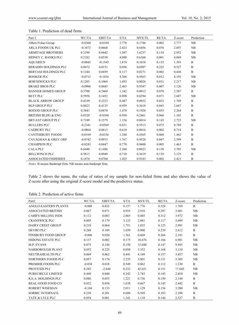
This section examines the Altman’s Z-score model to determine whether the high predictive ability that Altman claimed is still valid in recent business environment and further discuss the results. I use hold out samples to examine the original Altman’s Z-score and the result as follow:

This table shows the name, the value of ratios of my sample for failed firms and also shows the value of Z-score after using the original Z-score model and the predictive status.


89

Table 1. Prediction of dead firms

Part 2 WC/TA EBIT/TA S/TA MVE/TL RE/TA Z-score Prediction

Albert Fisher Group -0.0368 -0.0104 2.776 0.1746 0.002 2.777 NB

ARLA FOODS UK PLC -0.3472 0.0668 2.423 0.6456 0.076 2.697 NB

ARMITAGE BROTHERS 0.3199 0.0442 1.307 1.6237 0.110 2.952 NB

SIDNEY C. BANKS PLC 0.2182 0.0530 4.090 0.6360 0.001 4.869 NB

AQUARIUS -0.0045 -0.1545 1.674 0.1018 0.135 1.393 B

BERADIN HOLDINGS PLC 0.0672 0.0151 0.056 0.0507 0.222 0.527 B

BERTAM HOLDINGS PLC 0.1244 0.0459 0.117 0.0271 0.002 0.436 B

BOOKER PLC -0.0715 -0.1016 4.366 0.4563 0.012 4.193 NB

BORTHWICKS PLC 0.1203 0.1064 1.693 0.0026 0.031 2.217 NB

BRAKE BROS PLC -0.0906 0.0685 2.463 0.9347 0.007 3.126 NB

BANNER HOMES GROUP 0.3700 0.2469 1.242 0.0012 0.070 2.587 B

BETT PLC 0.5958 0.1452 0.898 0.8394 0.071 2.687 NB

BLACK ARROW GROUP 0.4339 0.2223 0.487 0.0032 0.022 1.769 B

BLP GROUP PLC 0.0623 0.4135 0.959 0.3618 0.043 2.667 B

BOGOD GROUP PLC 0.3843 0.0470 1.470 0.1920 0.055 2.264 B

BRITISH BLDG & ENG 0.0320 -0.0360 0.950 0.2461 0.066 1.101 B

BRYANT GROUP PLC 0.7109 0.1579 1.156 0.0014 0.145 2.723 NB

BULLERS PLC -0.2341 -0.0569 0.831 0.5513 0.075 0.789 B

CADBURY PLC -0.0864 0.0613 0.618 0.0016 0.002 0.714 B

CANTERBURY FOODS -0.0169 -0.0336 1.248 0.4565 0.060 1.462 B

CAVAGHAN & GREY GRP -0.0742 0.0915 1.767 0.9520 0.047 2.599 B

CHAMPION PLC -0.0243 0.0447 0.770 0.9600 0.005 1.463 B

CALA PLC 0.6440 0.1486 2.268 0.0023 0.138 3.703 NB

BELLWINCH PLC 0.5813 0.0949 0.710 0.3619 0.139 2.125 B

ASSOCIATED FISHERIES 0.1874 0.0704 1.425 0.9183 0.002 2.421 B

Notes. B means Bankrupt firm, NB means non-bankrupt firm.

Table 2 shows the name, the value of ratios of my sample for non-failed firms and also shows the value of Z-score after using the original Z-score model and the predictive status.

Table 2. Prediction of active firms

Part2 WC/TA EBIT/TA S/TA MVE/TL RE/TA Z-score Prediction

ANGLO-EASTERN PLANTS -0.008 0.032 0.157 1.776 0.324 1.769 B

ASSOCIATED BRITISH 0.067 0.071 0.935 2.910 0.297 3.401 NB

CARR'S MILLING INDS 0.112 0.083 2.865 0.485 0.312 3.972 NB

CRANSWICK PLC 0.005 0.179 3.123 2.081 0.117 5.099 NB

DAIRY CREST GROUP 0.210 0.064 1.751 1.035 0.125 2.991 NB

DEVRO PLC 0.288 0.109 1.039 0.908 0.239 2.612 B

FINSBURY FOOD GROUP -0.006 0.020 1.361 0.669 0.266 2.181 B

HIDONG ESTATE PLC 0.137 0.002 0.175 10.676 0.166 6.981 NB

M.P. EVANS 0.075 0.144 0.150 15.040 0.147 9.943 NB

NARBOROUGH PLANT 0.052 0.225 0.058 3.352 0.168 3.110 NB

NEUTRAHEALTH PLC 0.069 0.062 0.441 4.189 0.157 3.457 NB

NORTHERN FOODS PLC 0.057 0.174 2.235 3.801 0.121 5.305 NB

PREMIER FOODS PLC -0.038 0.018 0.549 0.862 0.112 1.230 B

PROVEXIS PLC 0.282 -2.644 0.232 42.651 0.151 17.645 NB

PURECIRCLE LIMITED 0.449 0.040 0.342 2.743 0.143 2.854 NB

R.E.A. HOLDINGS PLC 0.086 0.055 1.221 0.736 0.150 2.144 B

REAL GOOD FOOD CO 0.032 0.054 1.638 0.667 0.145 2.442 B

ROBERT WISEMAN -0.104 0.133 2.011 1.129 0.156 3.200 NB

SORBIC INTERNATL 0.238 0.201 0.680 0.569 0.103 2.108 B

TATE & LYLE PLC 0.054 0.081 1.341 1.110 0.144 2.527 B


90

UKRPRODUCT GROUP 0.126 0.177 2.037 2.668 0.132 4.537 NB

UNILEVER PLC 0.120 0.175 1.730 0.581 0.173 3.027 NB

UNIQ PLC -0.003 0.120 2.471 1.705 0.139 4.057 NB

WALCOM GROUP LTD 0.534 -0.184 0.712 39.814 0.187 24.890 NB

WYNNSTAY GROUP 0.229 0.060 2.338 1.064 0.149 3.633 NB

ZETAR PLC 0.026 0.089 1.386 1.665 0.133 2.883 NB

Table 3 shows the result of prediction, when comparing to the actual status. Also it indicates the error of prediction.

Table 3. The result of prediction

Actual Predicted Bankrupt Non-bankrupt Total number

Bankrupt 15 10 25

Non-bankrupt 8 17 25

This table shows the number of correct and error for prediction. Also, the correct rate of prediction.

Table 4. The correct rate for prediction

Correct Correct% Error Total number

Bankrupt 15 60% 10 25

Non-bankrupt 17 68% 8 25

Overall 32 64% 18 50

This table shows that the number of type I and type II errors separately and the percentage of each of them is account for the total error.

Table 5. The error of prediction

Type I error Type II error Total error

10 8 18

20% 16% 36%

Before interpreting the result of testing the original Z-score model, I give an introduction of the type I and type II error and the relationship of these two errors with the cut-off point of the prediction model. The concept of any prediction model is to find an appropriate position to allocate the cut-off point which minimises these misclassification errors. More specific, two types of misclassification errors in statistical process are type I error and type II errors. Type I error is rejecting a null hypothesis which is true while a type II error is fail to reject a null hypothesis which is false. In other words, type I error in prediction model means predicting a failed firm will not go bankrupt and type II error is predicting a non-failed firm to be bankrupt. To minimize the misclassification errors, it determined by the place of cut-off point, but if you minimize type I errors, it will raise the type II errors (or vice versa) since type I errors (%) plus type II errors (%) equal to 100%. Usually the institutions which granting a loan will place the cut-off point with the concept of prudent that to minimize the type I error is really importance. A small example of a bank might illustrate the balance of type I and type II errors. A bank wishes to evaluate a client’s loan to meet their repayment obligations should a loan be granted. A prediction model is used to predicting which firms will become bankrupt in loan period. The banks’ priority is to not lend any money to those firms which it suspects will become bankrupt or default on its obligations i.e., reduce the number of type I errors. It would be possible to completely remove any chance of such an error by raising the cut-off point of the model subjective high the bank in fact will not lend any money to any firms thus by failing to offer any loans to worthy applicants (type II errors) and not doing any business at all. Thus, although reducing type I errors is of high importance it must not be done at the expense of creating an unnecessary number of type II errors. A balance must be carefully make between type I errors and type II errors on the choice of the appropriate cut-off point of the prediction model.


91

Although Heine (2000) shows the type I accuracy of Z-score over 30 years is 82%-94%, but purely in consumer goods industry, the Z-score is not accurate as he claimed. As table 4.5 and 4.5 shown, there is only 80% type I accuracy, and the total error is 36% which including 20% type I error and 16% type II error. It shows little predictive ability of Original Altman’s Z-score. And Heine (2000) didn't show the M2 accuracy of Z-score and only mention of the M2 error of his study has increased to about 15%-20% which is not specific enough. For example, if the M2 accuracy is 16% the same M2 accuracy as my tested sample showed in Table 4:5 then the accuracy of the Z-score model will be only 64%. This result is not accurate as the original result which is 94% and 97% for Type I and Type II errors respectively. Also the accuracy of the M1 is not too low since I regard that the grey area between 1.8 and 2.67 set by Altman as the bankrupt groups. Thus, the accuracy of Z-score model is not as high as which claimed by Altman (1968) thereby the appropriate cut-off point still need to be reset to increase the accuracy. Since the low accuracy of the Altman’s Z-score might due to the appropriateness of the cut-off point and also the parameters of the Z-score model would shift over year, I run the multiple discriminant analysis to formulating the Original Altman’s Z-score by using recent more relevant data from good consumer industry.

4.3 The Methodology (Multiple Discriminant Analysis)

I am aiming to use multiple discriminate function analysis to establish the formula which can correctly distinguish the samples into bankrupt groups and non-bankrupt groups. To predicting the status of business, multiple discriminant Analysis undertakes the same task as multiple linear regression which is used to cases where the predictor (X) is an interval variable on the Y axis so that the combination of independent variables will, through the regression formula, produce estimated mean population numerical Y values for given values of weighted combinations of X values. Moreover, the dependent is classified with the predictors (independent variables) at interval level. And in this case, the predictor variables are Current working capital/ Total assets, Earning before interest and tax/ Total assets, Sales/ Total assets, Retained Earning/ Total asset and Market value of equity/ total liabilities. However, since logistic regression of those predictors can be of any level of measurement, multiple discriminant analysis unlike logistic regression that is confined to a dichotomous dependent variable, the discriminant analysis requires more than two groups. In this study, there are two groups which are bankrupt and non-bankrupt groups. A linear equation will classify the cases into either bankrupt group or non-bankrupt group which the group they belong to. The equation is express as follow:

Where D= discriminate function; V=the discriminate coefficient or weight for that variable;

=Working capital/ total asset; X =Earning Before Interest and Tax/total asset; X = Sales/ total asset;

=Retained earning/total asset; X =Market Value of Equity/Total liabilities.

In addition, the coefficients of predictors maximize the distance between the means of each group (bankrupt and non-bankrupt). Standardized discriminate coefficients can also be used and the larger the weights, the better the predictors.

4.3.1 The Assumptions

According to Agresti (1996), there are some major underlying assumptions of discriminate analysis are:

1) The observations are a random sample; Observations of my empirical study are collecting from the online resources in similar size and the same industry, they are randomly selected.

2) Each predictor variable is normally distributed. As I mentioned in previous section, the predictors which are financial ratios are unlikely to be exactly normality. But they can be nearly normality after data transformation into logistic. So I transform the data into logistic by SPSS transform function.

3) Each of the allocations for the dependent categories in the initial classification are correctly classified; Since the bankrupt firms are double check by the London Gazette while the data from non-bankrupt firms are download from the online resources, they have been correctly classified.

4) They must be at least two groups or categories, with each case belonging to only one group so that the groups are mutually exclusive and collectively exhaustive. In my study, all cases can be classified into either


92

bankrupt groups or non-bankrupt groups.

5) Each group or category must be well defined, clearly differentiated from any other groups and natural. Obviously, the bankrupt firms and non-bankrupt firms are easily identifiable gaps at the points of division and the groups are defined before collecting the data.

6) The attributes used to separate the groups should discriminate quite clearly between the groups so that group overlap is clearly non-existent or minimal;

This point has been proved by Altman’s Z-score model that the predictors (working capital/total assets, market value of equity/total liabilities, retained earnings/ total assets, sales/total assets, EBIT/total assets) can clearly distinguish between bankrupt and non-bankrupt groups, which has been mention at previous section.

7) Group sizes of the dependent should not be grossly different and should be at least five times the number of independent variables; From the formula, we can seen that the predictors( , , , , is five times the number of independent variable (D).

Thus, apart from the randomness and the normality of the data still not being tested, the properties of my observation and the situations of my study are subject to discriminate analysis. And I will test the hypothesis in the next section which is section 4.5.2.

4.3.2 Test of Hypothesis

This section will test the assumptions of discriminant analysis which have been mentioned before (in section 4.5.1) in order to minimize the measurement errors when using multiple discriminant analysis.

4.3.2.1 Test of Randomness

For the randomness assumption, it states that the observations should be random sample. Thus I test the randomness of the samples separately by using the Geary Test which is a nonparametric test that is used to test the randomness in sample data. The null hypothesis of the Geary Test is that the distributions of the two continuous data sets are the same, while the alternative hypothesis will be the opposite of the null hypothesis. If the P-value fall in the significant level, then the null hypothesis being rejected. And this means there is not enough evidence to say the sample are the same. Also I will double check the result by using the correlation within variables. The output of randomness test of data is shown as follow:

Where VAR0002, VAR0003, VAR0004, VAR0005 and VAR0006 repressed current working capital/total asset, EBIT/total asset, Sales/total asset, Market value of equity/total liabilities and Retained Earning of total asset respectively.

Table 6. Descriptive statistics of all predictors

N Mean Std. Deviation Minimum Maximum

VAR00002 50 .2128 .24379 -.36 .70

VAR00003 50 .0676 .13576 -.50 .25

VAR00004 50 1.2659 .70325 .14 4.52

VAR00005 50 1.5659 1.77122 .00 7.54

VAR00006 50 .0978 .05419 .00 .18

For information about Median, Kurtosis and Skewness of predictors, I show and illustrate them in the next section (table 8).

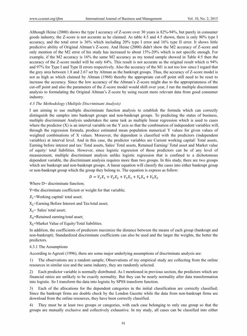
Table 7 shows that the significant of the Geary test and the null hypothesis of Geary test is that the distributions of the two continuous data sets are the same, which means they are not random. Thus, Geary test can be used to test randomness of the data and VAR0002, VAR0003, VAR0004, VAR0005 and VAR0006 repressed current working capital/total asset, EBIT/total asset, Sales/total asset, Market value of equity/total liabilities and Retained Earning of total asset respectively.


93

Table 7. Geary test

VAR00002 VAR00003 VAR00004 VAR00005 VAR00006

Test Value(a) .20 .10 1.15 .78 .10

Cases < Test Value 25 25 25 25 25

Cases >= Test Value 25 25 25 25 25

Total Cases 50 50 50 50 50

Number of Runs 23 26 26 6 6

Z -.857 .000 .000 -5.715 -5.715

Sig. (2-tailed) .391 1.000 1.000 .000 .000

Note. a Median.

As we can see from Geary test (table 7), in 5% significant level, the significances of variables that the current working capital/total assets, EBIT/total assets and the sales/total assets from the table which is 0.391, 1.000 and 1.000 individually are greater than 0.05, in other words, we reject the null hypothesis while there is insufficient evidence to support that the variables (market value of equity/total liabilities and retained Earning/total assets) have the same distribution. It indicates that, the variables (market value of equity/total liabilities and retained Earning/total assets) are random. And variables including current working capital/total assets, EBIT/total assets and the sales/total assets seem to be not random and it might due to firms with similar size and within same industries will have similar value in variables. However, this result is reasonable since these variables have little contribution to distinguish between failed firms and non-failed firms. Finally, the result indicates, the data of variables including current working capital/total asset, EBIT/total asset, Sales/total asset is random thereby they subject to the assumption of the discriminant analysis.

4.3.2.2 Test of Normality

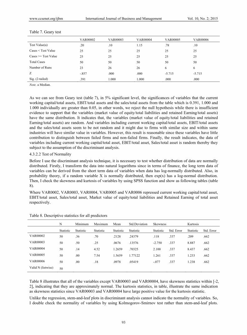
Before I use the discriminant analysis technique, it is necessary to test whether distribution of data are normally distributed. Firstly, I transform the data into natural logarithms since in terms of finance, the long term data of variables can be derived from the short term data of variables when data has log-normally distributed. Also, in probability theory, if a random variable X is normally distributed, then exp(x) has a log-normal distribution. Then, I check the skewness and kurtosis of variables by using SPSS function and show as following tables (table 8).

Where VAR0002, VAR0003, VAR0004, VAR0005 and VAR0006 repressed current working capital/total asset, EBIT/total asset, Sales/total asset, Market value of equity/total liabilities and Retained Earning of total asset respectively.

Table 8. Descriptive statistics for all predictors

N Minimum Maximum Mean Std.Deviation Skewness Kurtosis

Statistic Statistic Statistic Statistic Statistic Statistic Std. Error Statistic Std. Error

VAR00002 50 .36 .70 .2128 .24379 .118 .337 .209 .662

VAR00003 50 .50 .25 .0676 .13576 -2.750 .337 8.887 .662

VAR00004 50 .14 4.52 1.2659 .70325 2.100 .337 8.437 .662

VAR00005 50 .00 7.54 1.5659 1.77122 1.261 .337 1.233 .662

VAR00006 50 .00 .18 .0978 .05419 -.077 .337 1.238 .662

Valid N (listwise) 50

Table 8 illustrates that all of the variables except VAR00003 and VAR00004, have skewness statistics within [-2, 2], indicating that they are approximately normal. The kurtosis statistics, in table, illustrate the same indication as skewness statistics since VAR00003 and VAR00004 have large positive value for the kurtosis statistic.

Unlike the regression, stem-and-leaf plots in discriminant analysis cannot indicate the normality of variables. So, I double check the normality of variables by using Kolmogorov-Smirnov test rather than stem-and-leaf plots.


94

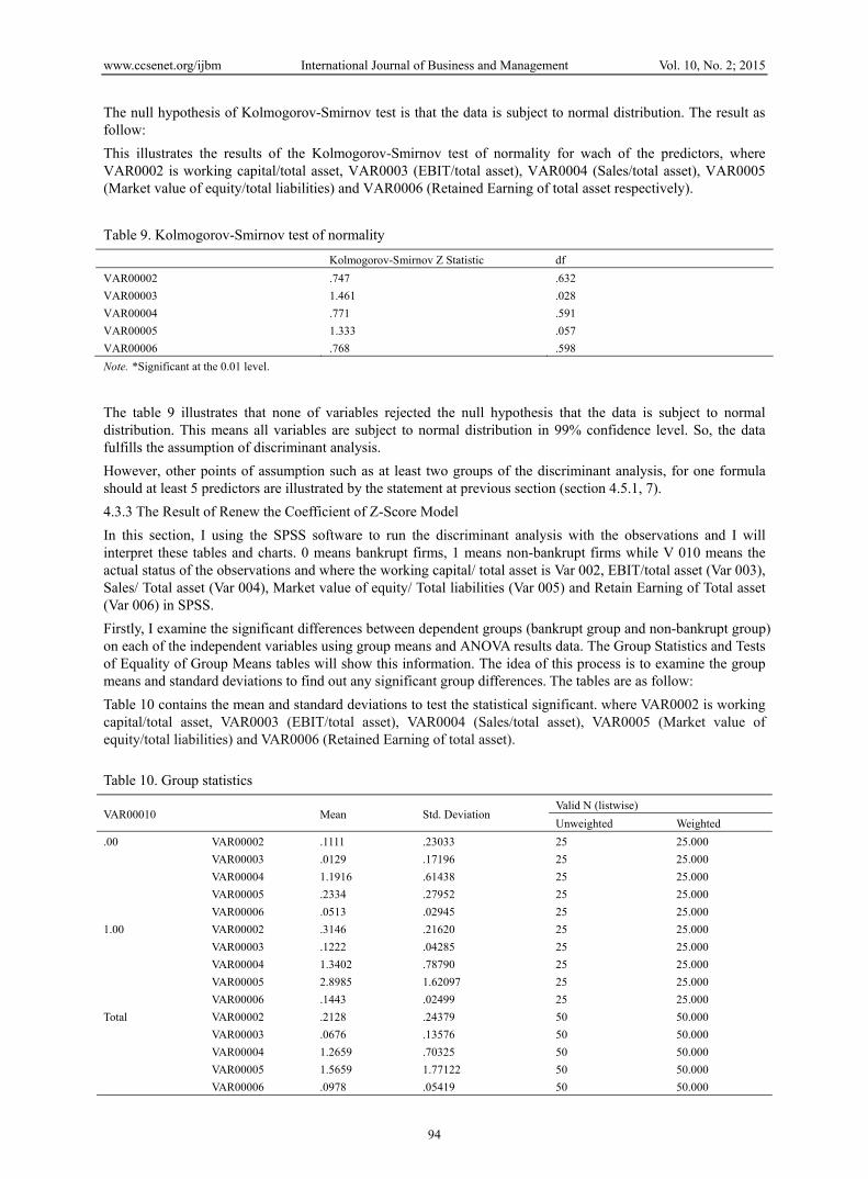
The null hypothesis of Kolmogorov-Smirnov test is that the data is subject to normal distribution. The result as follow:

This illustrates the results of the Kolmogorov-Smirnov test of normality for wach of the predictors, where VAR0002 is working capital/total asset, VAR0003 (EBIT/total asset), VAR0004 (Sales/total asset), VAR0005 (Market value of equity/total liabilities) and VAR0006 (Retained Earning of total asset respectively).

Table 9. Kolmogorov-Smirnov test of normality

Kolmogorov-Smirnov Z Statistic df

VAR00002 .747 .632

VAR00003 1.461 .028

VAR00004 .771 .591

VAR00005 1.333 .057

VAR00006 .768 .598

Note. *Significant at the 0.01 level.

The table 9 illustrates that none of variables rejected the null hypothesis that the data is subject to normal distribution. This means all variables are subject to normal distribution in 99% confidence level. So, the data fulfills the assumption of discriminant analysis.

However, other points of assumption such as at least two groups of the discriminant analysis, for one formula should at least 5 predictors are illustrated by the statement at previous section (section 4.5.1, 7).

4.3.3 The Result of Renew the Coefficient of Z-Score Model

In this section, I using the SPSS software to run the discriminant analysis with the observations and I will interpret these tables and charts. 0 means bankrupt firms, 1 means non-bankrupt firms while V 010 means the actual status of the observations and where the working capital/ total asset is Var 002, EBIT/total asset (Var 003), Sales/ Total asset (Var 004), Market value of equity/ Total liabilities (Var 005) and Retain Earning of Total asset (Var 006) in SPSS.

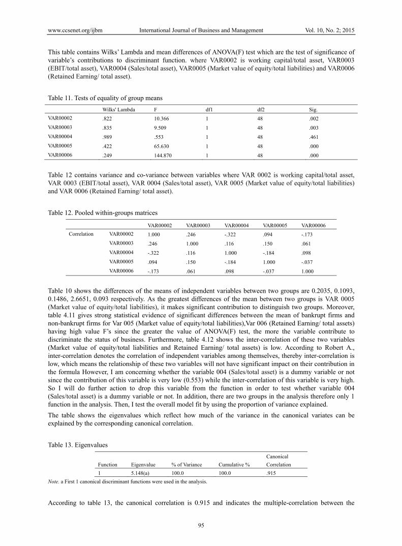
Firstly, I examine the significant differences between dependent groups (bankrupt group and non-bankrupt group) on each of the independent variables using group means and ANOVA results data. The Group Statistics and Tests of Equality of Group Means tables will show this information. The idea of this process is to examine the group means and standard deviations to find out any significant group differences. The tables are as follow:

Table 10 contains the mean and standard deviations to test the statistical significant. where VAR0002 is working capital/total asset, VAR0003 (EBIT/total asset), VAR0004 (Sales/total asset), VAR0005 (Market value of equity/total liabilities) and VAR0006 (Retained Earning of total asset). Table 10. Group statistics

VAR00010 Mean Std. Deviation Valid N (listwise)

Unweighted Weighted

.00 VAR00002 .1111 .23033 25 25.000

VAR00003 .0129 .17196 25 25.000

VAR00004 1.1916 .61438 25 25.000

VAR00005 .2334 .27952 25 25.000

VAR00006 .0513 .02945 25 25.000

1.00 VAR00002 .3146 .21620 25 25.000

VAR00003 .1222 .04285 25 25.000

VAR00004 1.3402 .78790 25 25.000

VAR00005 2.8985 1.62097 25 25.000

VAR00006 .1443 .02499 25 25.000

Total VAR00002 .2128 .24379 50 50.000

VAR00003 .0676 .13576 50 50.000

VAR00004 1.2659 .70325 50 50.000

VAR00005 1.5659 1.77122 50 50.000

VAR00006 .0978 .05419 50 50.000


95

This table contains Wilks’ Lambda and mean differences of ANOVA(F) test which are the test of significance of variable’s contributions to discriminant function. where VAR0002 is working capital/total asset, VAR0003 (EBIT/total asset), VAR0004 (Sales/total asset), VAR0005 (Market value of equity/total liabilities) and VAR0006 (Retained Earning/ total asset).

Table 11. Tests of equality of group means

Wilks' Lambda F df1 df2 Sig.

VAR00002 .822 10.366 1 48 .002

VAR00003 .835 9.509 1 48 .003

VAR00004 .989 .553 1 48 .461

VAR00005 .422 65.630 1 48 .000

VAR00006 .249 144.870 1 48 .000

Table 12 contains variance and co-variance between variables where VAR 0002 is working capital/total asset, VAR 0003 (EBIT/total asset), VAR 0004 (Sales/total asset), VAR 0005 (Market value of equity/total liabilities) and VAR 0006 (Retained Earning/ total asset).

Table 12. Pooled within-groups matrices

VAR00002 VAR00003 VAR00004 VAR00005 VAR00006

Correlation VAR00002 1.000 .246 -.322 .094 -.173

VAR00003 .246 1.000 .116 .150 .061

VAR00004 -.322 .116 1.000 -.184 .098

VAR00005 .094 .150 -.184 1.000 -.037

VAR00006 -.173 .061 .098 -.037 1.000

Table 10 shows the differences of the means of independent variables between two groups are 0.2035, 0.1093, 0.1486, 2.6651, 0.093 respectively. As the greatest differences of the mean between two groups is VAR 0005 (Market value of equity/total liabilities), it makes significant contribution to distinguish two groups. Moreover, table 4.11 gives strong statistical evidence of significant differences between the mean of bankrupt firms and non-bankrupt firms for Var 005 (Market value of equity/total liabilities),Var 006 (Retained Earning/ total assets) having high value F’s since the greater the value of ANOVA(F) test, the more the variable contribute to discriminate the status of business. Furthermore, table 4.12 shows the inter-correlation of these two variables (Market value of equity/total liabilities and Retained Earning/ total assets) is low. According to Robert A., inter-correlation denotes the correlation of independent variables among themselves, thereby inter-correlation is low, which means the relationship of these two variables will not have significant impact on their contribution in the formula However, I am concerning whether the variable 004 (Sales/total asset) is a dummy variable or not since the contribution of this variable is very low (0.553) while the inter-correlation of this variable is very high. So I will do further action to drop this variable from the function in order to test whether variable 004 (Sales/total asset) is a dummy variable or not. In addition, there are two groups in the analysis therefore only 1 function in the analysis. Then, I test the overall model fit by using the proportion of variance explained.

The table shows the eigenvalues which reflect how much of the variance in the canonical variates can be explained by the corresponding canonical correlation.

Table 13. Eigenvalues

Function Eigenvalue % of Variance Cumulative %

Canonical

Correlation

1 5.148(a) 100.0 100.0 .915

Note. a First 1 canonical discriminant functions were used in the analysis.

According to table 13, the canonical correlation is 0.915 and indicates the multiple-correlation between the


96

independent variables and the discriminant function. Thus, it indicates that the model explains 83.7% (the square of 0.915) of the variance in the discriminant equation.

The table 14 shows the Wilks’ Lambda to test the significant differences between groups of the centroid means on the independent variables.

Table 14. Wilks' lambda

Test of Function(s)

Wilks'

Lambda Chi-square df Sig.

1 .163 82.637 5 .000

To test the significant of the discriminant function, I use Wilk’s Lambda which is a measure of the significant difference between groups of the centroid means on the predictors (independent variables). According to George H., the smaller the value of Wilks’ Lambda, the greater the differences between the centroid mean. The table 14 shows Wilks’ lambda is 0.163 and indicates that a highly significant function since in 95% confidence interval, P value of the test is 0.00 which means not reject the hypothesis and provides the proportion of total variability not explained so it is 16.3%.

The table 15 shows the contribution of independent variables to the discriminant function according to the observations and where VAR0002 is working capital/total asset, VAR0003 (EBIT/total asset), VAR0004 (Sales/total asset), VAR0005 (Market value of equity/total liabilities) and VAR0006 (Retained Earning/ total asset).

Table 15. Standardized canonical discriminant function coefficients

Function

1

VAR00002 .372

VAR00003 -.052

VAR00004 .194

VAR00005 .554

VAR00006 .835

After that, I would like to see the discriminant coefficients (weights) in the function. Table 4.15 shows an index of the importance of each predictor like the standardized regression coefficients (beta’s) did in multiple regression. Regarding the sign indicates the direction of the relationship, I consider the contribution of predictors with absolute value. The working capital/total asset, the market value of equity /total liabilities and retained earnings with large coefficients represent those that have strongly predictive ability to distinguish the bankrupt and non-bankrupt group while EBIT/total asset and Sales/ total asset are less successful as predictors.

The table 16 shows the correlations between the five observed discriminating variables and the discriminant function and where VAR0002 is working capital/total asset, VAR0003 (EBIT/total asset), VAR0004 (Sales/total asset), VAR0005 (Market value of equity/total liabilities) and VAR0006 (Retained Earning/ total asset).

Table 16. Structure matrix

Function

1

VAR00006 .766

VAR00005 .515

VAR00002 .205

VAR00003 .196

VAR00004 .047

However, regard to the accuracy, researchers use the structure matrix rather than standardized canonical


97

discriminant function coefficients table to indicate the relative importance of the predictors. The coefficients of structure matrix (table 16) serve like factor loadings in factor analysis. According to Agresti (1996), the general cut-off point between important and less important variables is 0.30. In this case, the retained earnings/ total assets and market value of equity/ total liabilities are more important while the sales/ total assets ratio is the weakest predictor and consistent with the previous judgment from the table Tests of Equality of Group Means (Table 11).

The table shows the coefficient of the discriminant function based on the observations and where VAR0002 is working capital/total asset, VAR0003 (EBIT/total asset), VAR0004 (Sales/total asset), VAR0005 (Market value of equity/total liabilities) and VAR0006 (Retained Earning/ total asset).

Table 17. Canonical discriminant function coefficients

Function

1

VAR00002 1.667

VAR00003 -.416

VAR00004 .274

VAR00005 .477

VAR00006 30.561

(Constant) -4.410

I can obtain the discriminant function from the canonical discriminant function coefficient (table 17) and which express as: 1.667 2 4.16 3 0.274 4 0.477 5 30.561 6 4.41

where VAR0002 is working capital/total asset, VAR0003 is EBIT/total asset, VAR0004 is Sales/total asset, VAR0005 is Market value of equity/total liabilities and VAR0006 is Retained Earning/ total asset.

Producing a score for D (discriminant score) for each case using the discriminante function, then case with D values smaller than the cut-off value are classified as belonging to one group while those with values greater are classified into the other group. In this case, the one with smaller D value belongs to bankrupt firm while the one with greater D value belongs to non-bankrupt firm.

The tables 18 shows the group means on the discriminant analysis where VAR00010 means the status of the firms, .00 means the bankrupt firms while 1.00 means the non-bankrupt firms.

Table 18. Functions at group centroids

VAR00010

Function

1

.00 -2.223

1.00 2.223

To identify the cut-off point, the group centroids can provide information about that. The group centroid is the group means of the predictor variables in bankrupt group and non-bankrupt group. The table 18 shows that bankrupt firms have a mean of -2.223 while non-bankrupt firms have a mean of 2.223. Firms have scores close to a centroid and will be predicted as belonging to that group. In this case, the one with D score near to -2.223 belongs to bankrupt firm while the one with D score near to 2.223 belongs to non-bankrupt firm.

The table shows the accuracy of the original and cross validated. The cross validated is a technique to measure how accuracy of the prediction model in practice.


98

Table 19. Classification results

VAR00010

Predicted Group Membership

Total .00 1.00

Original Count .00 25 0 25

1.00 0 25 25

% .00 100.0 .0 100.0

1.00 .0 100.0 100.0

Cross-validated(a) Count .00 24 1 25

1.00 3 22 25

% .00 96.0 4.0 100.0

1.00 12.0 88.0 100.0

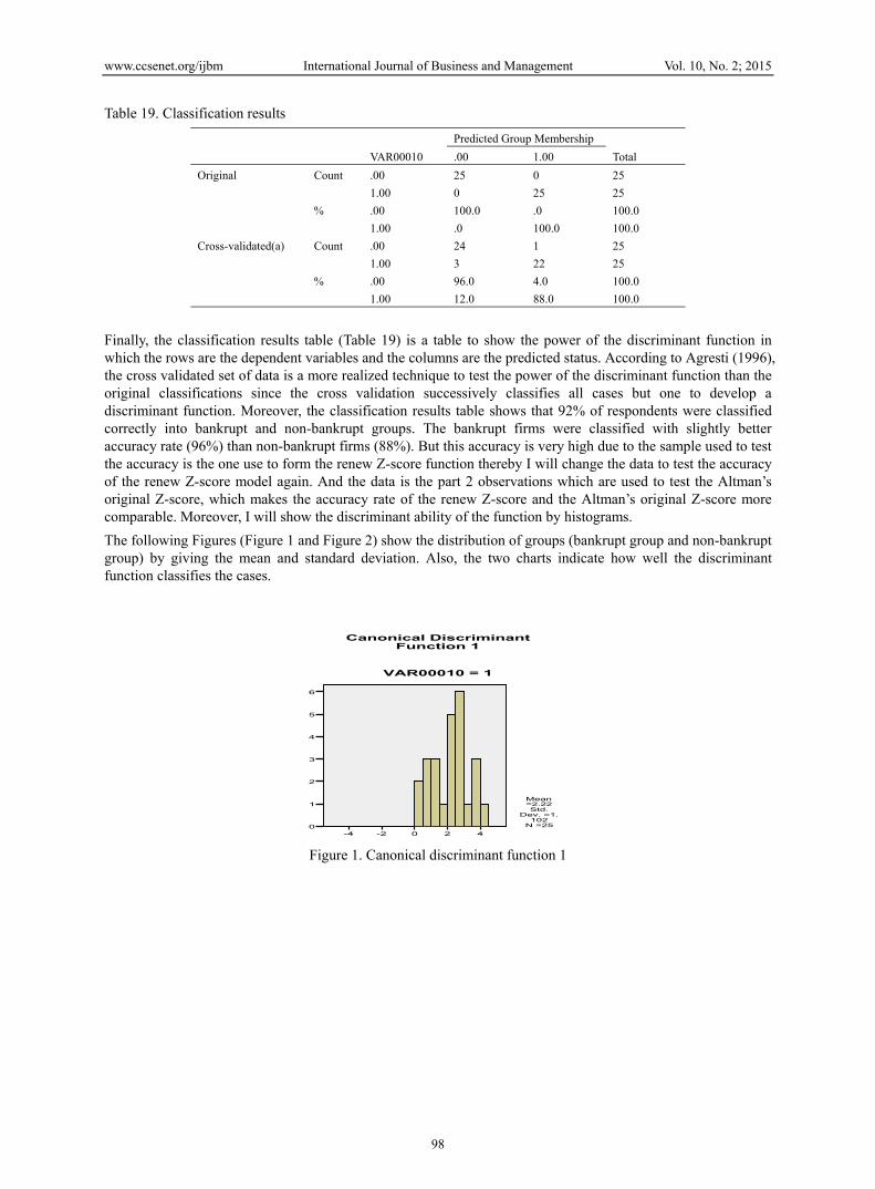
Finally, the classification results table (Table 19) is a table to show the power of the discriminant function in which the rows are the dependent variables and the columns are the predicted status. According to Agresti (1996), the cross validated set of data is a more realized technique to test the power of the discriminant function than the original classifications since the cross validation successively classifies all cases but one to develop a discriminant function. Moreover, the classification results table shows that 92% of respondents were classified correctly into bankrupt and non-bankrupt groups. The bankrupt firms were classified with slightly better accuracy rate (96%) than non-bankrupt firms (88%). But this accuracy is very high due to the sample used to test the accuracy is the one use to form the renew Z-score function thereby I will change the data to test the accuracy of the renew Z-score model again. And the data is the part 2 observations which are used to test the Altman’s original Z-score, which makes the accuracy rate of the renew Z-score and the Altman’s original Z-score more comparable. Moreover, I will show the discriminant ability of the function by histograms.

The following Figures (Figure 1 and Figure 2) show the distribution of groups (bankrupt group and non-bankrupt group) by giving the mean and standard deviation. Also, the two charts indicate how well the discriminant function classifies the cases.

Figure 1. Canonical discriminant function 1

420-2-4

6

5

4

3

2

1

0

VAR00010 = 1

Canonical Discriminant Function 1

Mean =2.22

Std. Dev. =1.

102N =25


99

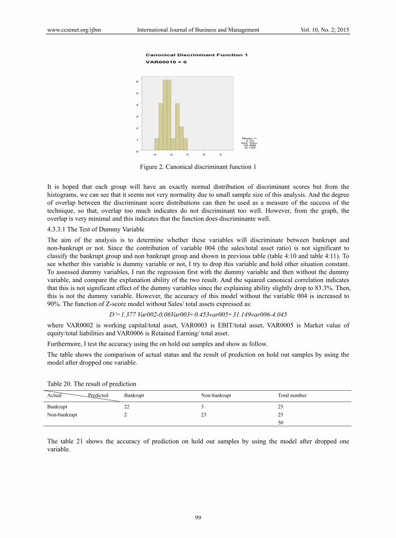
Figure 2. Canonical discriminant function 1

It is hoped that each group will have an exactly normal distribution of discriminant scores but from the histograms, we can see that it seems not very normality due to small sample size of this analysis. And the degree of overlap between the discriminant score distributions can then be used as a measure of the success of the technique, so that, overlap too much indicates do not discriminant too well. However, from the graph, the overlap is very minimal and this indicates that the function does discriminante well.

4.3.3.1 The Test of Dummy Variable

The aim of the analysis is to determine whether these variables will discriminate between bankrupt and non-bankrupt or not. Since the contribution of variable 004 (the sales/total asset ratio) is not significant to classify the bankrupt group and non bankrupt group and shown in previous table (table 4:10 and table 4:11). To see whether this variable is dummy variable or not, I try to drop this variable and hold other situation constant. To assessed dummy variables, I run the regression first with the dummy variable and then without the dummy variable, and compare the explanation ability of the two result. And the squared canonical correlation indicates that this is not significant effect of the dummy variables since the explaining ability slightly drop to 83.3%. Then, this is not the dummy variable. However, the accuracy of this model without the variable 004 is increased to 90%. The function of Z-score model without Sales/ total assets expressed as:

D’=1.377 Var002-0.06Var003+0.453var005+31.149var006-4.045

where VAR0002 is working capital/total asset, VAR0003 is EBIT/total asset, VAR0005 is Market value of equity/total liabilities and VAR0006 is Retained Earning/ total asset.

Furthermore, I test the accuracy using the on hold out samples and show as follow.

The table shows the comparison of actual status and the result of prediction on hold out samples by using the model after dropped one variable.

Table 20. The result of prediction


Bankrupt 22 3 25


50

The table 21 shows the accuracy of prediction on hold out samples by using the model after dropped one variable.

420-2-4

6

5

4

3

2

1

0

VAR00010 = 0

Canonical Discriminant Function 1

Mean =-2.22

Std. Dev. =0.886N =25


100

Table 21. The accuracy of prediction

Correct Correct% Error overall

Bankrupt 22 88% 3 25


45 90% 5 50

The table 22 shows that the number and percentage of type I and type II errors separately while used the prediction model after dropped one variable on the hold out samples.

Table 22. The error of prediction


3 2 5

6% 4% 10%

As the tables (Table 21 and 22) above show that, the accuracy of the model without var004 (the sales/ total assets) on the hold out samples is 90% which is slightly higher than 88% which mention at previous. This interprets when used models on the same hold out samples individually, the prediction model dropped one variable has a slightly higher accurate rate than the model which has the same variables as original Z-score model by holding other situations constant.

The table 23 shows the canonical correlation of equation, which use to measure the explanation ability of the equation. The square of 0,913 is used to illustrate the explanation ability of the equation and the greater the more explanation ability, the maximum is 100%.

Table 23. Eigenvalues

Function Eigenvalue % of Variance Cumulative % Canonical

Correlation

1 4.990(a) 100.0 100.0 .913

However, as we can see from the table 23, the explanation ability of equation slightly decreased to 83.3% (0.913 %) after dropped one variable. It also indicates that the var004 (the sales/ total assets) is not a dummy variable since without it, the explanation ability of equation will fall. In addition, the assumption of using the discriminant analysis confine that the independent variables are at least five times much as the dependent variable. If I drop the one variable, then I violate the assumption of using discriminant analysis thereby I keep the variable 004 (the sales/total assets) although the accuracy will slightly fall.

4.3.3.2 The Accuracy of the Renew Z-Score

In this section, I will use the hold out samples which is part 2 samples (hold out samples) to test the accuracy of renewed Z-score.

If the cut-off point is the average of the two groups centroid which is 0, the situation will as follow:

The table shows the comparison of actual status and the result of prediction on hold out samples by using the renewed Z-score prediction model and when the cut-off point is 0.

Table 24. The result of prediction on renewed Z-score model


Bankrupt 21 4 25


50

The table shows the accuracy of prediction on hold out samples by using renewed coefficients Z-score prediction model, when the cut-off point is 0.


101

Table 25. The accuracy of renewed Z-score prediction model

Correct Correct% Error



44 88% 6 50

The table 26 shows that the number and percentage of type I and type II errors separately while used the renewed coefficients of Z-score prediction model on the hold out samples.

Table 26. The errors of prediction


4 2 6

8% 4% 12%

From the above tables (Table 24, 25 and 26), we can see that, the accuracy of this model is as good as the accuracy show on the part 1 sample which is the one use to form the formula. As table 25 shown, the overall accuracy of this new model is 88% which including accuracy of type I error is 84% when the accuracy of type II error is 92%. It indicates that if the one use this model for granting out the load, it is not prudent enough, since the accuracy of type I error is only 84% and they can increase the accuracy of type I error by setting a higher cut-off point. But if they increase the cut-off point, the accuracy of type II error will drop, so it is necessary for the one who used this model to set an appropriate cut-off point to trade off the balance between type I error and type II error for their purpose.

4.4 Comparison of Altman’s Original Z-Score and Renewed Z-Score Model

In this section I am going to make a comparison of the Altman’s original Z-score model and the renewed Z-score model in UK and in the consumer goods industry. The comparison is including the accuracy of the model and the contribution of variables to the model.

4.4.1 The Accuracy

I use these two models on the hold out sample individually and given the result as follow:

The original Z-score model:

This table 27 shows the result of prediction on hold out samples using the original Z-score prediction model, when comparing to the actual status. Also it indicates the error of prediction.

Table 27. The result of using the original Z-score prediction model


Bankrupt 15 10 25


This table 28 shows the number of correct and error for prediction. Also, the correct rate of the original Z-score prediction model.

Table 28. The correct rate for the original Z-score model

Correct Correct% Error Total number

Bankrupt 15 60% 10 25


Overall 32 64% 18

This table shows that the number of type I and type II errors separately and the percentage of each of them is account for the total error.


102

Table 29. The error of the original Z-score prediction model


10 8 18

20% 16% 36%

The renewed Z-score model:

The table 30 shows the comparison of actual status and the result of prediction on hold out samples by using the renewed Z-score prediction model and when the cut-off point is 0.

Table 30. The result of prediction on renewed Z-score model


Bankrupt 21 4 25


50

The table shows the accuracy of prediction on hold out samples by using renewed coefficients Z-score prediction model, when the cut-off point is 0.

Table 31. The accuracy of renewed Z-score prediction model

Correct Correct% Error



44 88% 6 50

The table shows that the number and percentage of type I and type II errors separately while used the renewed coefficients of Z-score prediction model on the hold out samples.

Table 32. The errors of renewed Z-score prediction model


4 2 6

8% 4% 12%

As we can see from the tables (table 28 and 31) that, while the overall accuracy of the original Z-score is 64%, the overall accuracy of the renewed Z-score is 88%. It means the renewed Z-score model increase 24% accuracy by using the recent data to run the discriminant analysis. More specific, as table 29 and 31 shown, the accuracy of type I error is increased from 80% to 92% whist the accuracy of the M2 rise from 84% to 96%. However, compared to the accuracy of Z-score model which Altman claimed, the accuracy of the renewed Z-score is still not as high as 97%.

4.4.2 The Variables

Since I use the variables the same as Altman’s original Z-score model, so the explanation of these variables taken from Altman (1968) is as follow:

1) Net Working Capital/ Total Assets

This variable is a measure of the net liquid assets of the firm relative to the total capitalization. Net Working Capital is defined as the difference between current assets and current liabilities. Liquidity and size characteristics are explicitly considered.

2) Retained Earning/ Total Assets

This variable is measure of cumulative profitability over time was cited earlier as one of the “new” ratios. The age of a firm is implicitly considered in this ratio.


103

3) Earnings Before Interest and Taxes/Total Assets

This variable is a measure of the true productivity of the firm’s assets, abstracting from any tax or leverage factors and calculated by dividing the total assets of a firm into its earnings before interest and tax reductions. The earning power of its asset is implicitly considered in this ratio.

4) Market Value of Equity/ Book Value of Total Debt

This ratio shows how much the firm’s assets can decline in value (measured by market value of equity plus debt) before the liabilities exceed the assets and the firm becomes insolvent.

5) Sales/Total Assets

This variable is a measure of management’s capability in dealing with competitive conditions (Atman, 1968, p. 594).

Comparing to the original Z-score model, coefficient of net working capital/ total assets, market value of equity/ total liabilities and sales/total assets in the renewed Z-score model is slightly increased that means they have greater contribution to prediction of bankrupt firms. However, the coefficient of the sale/total asset become negative which means this variable have opposite impact on the Z-score. This might due to the industries characteristic and majority of sales is credit sales recently. and if it is credit sales, then it is easy to become bad debts so the cash flow or the liquidity of cash would have problem. and the industries including good consumer and the food producer have the characteristic that they have high proportion of assets and if the turnover of sales cannot cover the assets which been require for the next period, the liquidity of cash would have problem. In this sense, the sales/ total assets have opposite impact on the Z-score. and which means the higher rate of the sales/ total assets, the higher probability the firm going to bankrupt. The coefficient of retained earing is significant increased in the renewed Z-score model and it might due to the more earning they accumulated, the older the firm and the less probability of a firm going bankrupt. Moreover, it is perhaps people would like to believe the old firm are more reliable and became more conservative due to the business environment has a great change during the last two decades. Thus, there are some significant changes about the contribution of the variables to the Z-score to predict bankruptcy.

5. Conclusion The dissertation has discussed the prediction model of bankruptcy firm due to insolvency in UK and within the consumer goods industry during these 20 years period. And I doing the key literature review on the development of bankruptcy prediction model, how these models work and its application by stakeholders and how successful of them. The most important is the concepts of these models and the advantage and disadvantage of these models. After that, I provided my empirical evident to support my hypothesis that the use of Altman’s Z-score in UK is out of date and need to be renewed to improve its accuracy. From a sample of 50 samples within the UK which including half of them is bankrupt firms and a matched half of them is non-bankrupt firms. The Altman’s Z-score were test and the result is 64% accuracy rate for bankrupt firms and non-bankrupt firms. This result shows that Altman’s Z-score has a poor predictive ability when applied to consumer goods in UK compared to the accuracy rate that Altman claimed.

Finally, I use discriminant analysis to renew the coefficient of the original Z-score model and found that one of the variables (sales/total assets) is not significant to the two groups. and I test the function with or without this variable for more accuracy and explanatory of function. and I found that this variable (the sales/ total assets) is not the dummy variable since the ability of explanting equation has slightly dropped when without this variable in the equation thereby I remain use five variables (current working capital/total assets, Earning before interest and tax/ total assets, Retained Earning/ total assets, sales/ total assets, market value of equity/ total liabilities) which the same as the original Z-score model. The renewed Z-score model out-performs the original Z-score model by increased 24% accuracy in bankruptcy prediction of consumer goods. Although the success rate of Z-score model is still not as good as the Altman claimed (97%), this study provides evidence that the Altman’s Z-score is not valid for consumer goods industry and the renewed Z-score out-performs the original one.

5.1 The Limitations

There are several limitations when doing the empirical study. The most important limitation was the sample size and the variables. If giving more time for study, I might collect more information of samples and also more firms within the period of study and increase the sample size. Also I can add some variable into the function and do more research on the variable inter-correlation. One more limitation is my economic and mathematics knowledge. Although the growth rate of the value and the market premium will cause measurement error on the result, I ignore these two factors since they are hard to adjust due to my math and economic knowledge


104

limitation. and if I simple discounted the value by the growth rate or inflation rate, it is incomparable with other firms failed in different point of time. Finally, it is the self-defeating efficacy problem. If the model can fully detect the firm will go bankrupt, then the investors of the firm might use the selfish strategy. For example, investing in high risk projects, incentive to under-invest or paid out higher dividends. These kinds of action might collapse the firm when the firm in financial distress. However, when the management of the firm detected the firm will failed, they might use active strategies, such as merge the firm with other firm, buy out strategies. In this case, the firm might not bankrupt even predicted it will go bankrupt. Thus, the accuracy of the prediction model was reduced by this kind of effect.

Due to the above limitations, to enhance its accuracy of prediction, the extra financial ratio might need to be analyzed and I would suggest that combining use the Z-score renewed by recent data and financial ratio analysis to predict firm’s financial distress within consumer goods industry in UK

5.2 Extensions

From the limitation, I suggest the extension is to increase the sample size and try different combination of independent variables (since some independent variables might not relevant to the recent business environment) using the same techniques to re-formulate the Z-score. Further extension can do more comparison on the several year data using on the Z-score model and observe the predictive ability of these different years. And also the observations could extend to wider industries and comparing contribution of variables in different industries since different industries have different characteristics. Moreover, it can extend to smaller, private firms and also firms from other countries. In terms of the techniques, logit and probit models, rescursive partitioning and neural networks can be used even they are complex. Further study can focus on the variables since the Z-score model is used the accounting data which in lagged accounting data. Then, some methods or some market variable taken economic trends into account are need for further study since these variables and methods can compensated the lagged accounting data and more caution. And developing the accounting variables in Z-score, it calls for more market specific variables such as the share price or P/E ratio (Price/Earning) of the firm. However, it is another area relative to the prediction model. I hope, this dissertation can form the concept of further study and the extension above can be investigated further.

References Altman, E. I. (1984). The Success of Business Failure Prediction Models. Journal of Banking and Finance, 8,

171–198. http://dx.doi.org/10.1016/0378-4266(84)90003-7

Agresti, A. (1996). An Introduction to Categorical Data Analysis. John Wiley and Sons.

Aharony, J., Jones, C. O., & Swary, I. (1980). An analysis of risk and return characteristics of corporate bankruptcy using capital market data. Journal of Finance, 1001–1016. http://dx.doi.org/10.1111/j.1540-6261.1980.tb03516.x

Alexander, S. S. (1949). The Effect of Size of Manufacturing Corporation on the Distribution of the Rate of Return. Review of Economics and Statistics, 229–235. http://dx.doi.org/10.2307/1927749

Altman, E. I. (1968). Financial Ratios, Discriminant Analysis and the Prediction of Corporate Bankruptcy. Journal of Finance, 23(4), 589–609. http://dx.doi.org/10.1111/j.1540-6261.1968.tb00843.x

Altman, E. I. (1983). Accounting Implication of Failure Prediction Models. Journal of Accounting, Auditing and Finance, 4–19.

Altman, E. I., & Haldeman, R. G., & Narayanan, P. (1977). ZETA analysis. A new model to identify bankruptcy risk of corporations. J. Banking and Finance, 1, 29–54. http://dx.doi.org/10.1016/0378-4266(77)90017-6

Anthony, W. (2009). Corporate insolvency and its prediction: 40 years of the Z-score, but does it work today?

Back, B., Laitinen, T., & Sere, K. (1995). Neural networks and bankruptcy prediction: funds flows. Accrual Ratios and Accounting Data, Series A-4, Turku School of Economics and Business Administration, Turku.

Beaver, W. (1966). Financial Ratios as Predictors of Failures. Empirical Research in Accounting. Journal of Accounting Research. http://dx.doi.org/10.2307/2490171

Deakin, E. (1972). A Discriminant Analysis of Predictors of Business Failure. Journal of Accounting Research. http://dx.doi.org/10.2307/2490225

Deakin, E. (1977). Business Failure Prediction: An Empirical Analysis. Financial crises: Institutions and Markets in a Fragile Environment. New York: Wiley.

Falkenstein, E., Andrew, B., & Lea, V. C. (2000). Risk Calc TM for private Compan: Moody’s Default Model.


105

Moody’s Investors Service Global Credit Research.

Fan, A., & Palaniswami, M. (2000). Selecting bankruptcy predictors using a support vector machine approach. In Proceedings of the IEEE–INNS–ENNS. International Joint Conference on Neural Networks, 6, 354–359. http://dx.doi.org/10.1109/IJCNN.2000.859421

FitPatrick, P. J. (1932). A Comparison of Ratios of Successful Industrial Enterprises with Those of Failed Firms. Certified Public Accountant.

Foster, D. P., & Stine, R. A. (2004). Variable selection in data mining: building a predictive model for bankruptcy. Journal of the American Statistical Association, 99(466), 303–313. http://dx.doi.org/10.1198/016214504000000287

George, H. D. (1984). Introduction to multivariate analysis. Thousand Oaks, CA: Sage Publications. Chapter 5 covers classification procedures and discriminant analysis.

Heine, M. L. (2000). Predicting Financial Distress of Companies: Revisiting the Z-score and ZETA Models. New York: University July 2000.

Hemscott Company Guru. (2010). Retrieved from http://www.hemscott.com/guru2/html/guru-product-tour.htm

International Monetary Fund. (1988). Retrieved from http://www.imf.org/external/index.htm

Jardin, P., & Séverin, E. (2011). Predicting corporate bankruptcy using a self-organizing map: an empirical study to improve the forecasting horizon of a financial failure model. Decision Support Systems, 51(3), 701–711. http://dx.doi.org/10.1016/j.dss.2011.04.001

Marais, M. L., Patel, J., & Wolfson, M. (1984). The experimental design of classification models: an application of recursive partitioning and bootstrapping to commercial bank loan classifications. Journal of Accounting Research, 22, 87–113. http://dx.doi.org/10.2307/2490861

Merwin, C. (1942). Financing Small Corporations in Five Manufacturing Industries, 1926-36. New York: National Bureau of Economic Research.

Morris, R. (1997). Early warning indicators of corporate failure. Ashgate Publishing. London Gazette. Retrieved from http://www.london-gazette.co.uk

Mukkamala, S., Tilve, D. D., & Sung, A. H. (2006). Computational intelligent techniques for financial distress detection. International Journal of Computational Intelligence Research, 2(1), 60–65. http://dx.doi.org/10.5019/j.ijcir.2006.44

Ohlson, J. A. (1980). Financial Ratios and the Probabilistic Prediction of Bankruptcy. Journal of Accounting Research, 18(1), 109–131. http://dx.doi.org/10.2307/2490395

Olson, D. L., Delen, D., & Meng, Y. (2012). Comparative analysis of data mining methods for bankruptcy prediction. Decision Support Systems, 52(2), 464–473. http://dx.doi.org/10.1016/j.dss.2011.10.007

Robert, A. Y. (2007). Common Correlation and Reliability Analysis with SPSS for Windows. Statistics and Social Science Group, Academic Computing Facility, New York University.

Sarkar, S., & Sriram, R. S. (2001). Bayesian models for early warning of bank failures. Management Science, 47(11), 1457–1475. http://dx.doi.org/10.1287/mnsc.47.11.1457.10253

Serrano-Cinca, C. (1993). Self organizing neural networks for financial diagnosis. Decision Support Systems, 17(3), 227–238. http://dx.doi.org/10.1016/0167-9236(95)00033-X

Smith, R. F., & Winakor, A. H. (1935). Changes in Financial Structure of Unsuccessful Corporations. Bureau of Business Research.

Taffler, R. J. (1983). The Assessment of Company Solvency and Performance Using a Statistical Model. Accounting and Business Research. http://dx.doi.org/10.1080/00014788.1983.9729767

Taffler, R. J. (1995). The Use of the Z-score Approach in Practice. Centre for Empirical Research in Finance and Accounting, City University Business School Working Paper.

Taffler, R. J., & Tisshaw, H. (1977). Going, Going, Gone-Four Factors Which Predict. Accountancy.

Taffler, R., & Agerwal, V. (2005). Twenty-five years of the Taffler Z-score model: does it really have predictive ability? Accounting and Business Research, 37(4), 285–300.

Taffler. R. J. (1982). Forecasting company failure in the UK using discriminant analysis and financial ratio data. Journal of Royal Statistical Society, 145(3), 342–358. http://dx.doi.org/10.2307/2981867


106

Tam, K. Y., & Kiang, M. Y. (1992). Managerial applications of neural networks: the case of bank failure predictions. Management Science, 38(7), 926–947. http://dx.doi.org/10.1287/mnsc.38.7.926

The Companies Act. (2010). Retrieved from http://www.legislation.gov.uk/ukpga/2006/46/pdfs/ukpga_20060046_en.pdf

Thomson One Banker. (2010). Retrieved from http://banker.thomsonib.com/

Wilcox, J. W. (1976). The Gambler’s Ruin Approach to Business Risk. Sloan Management Review, 18(1), 33.

Copyrights Copyright for this article is retained by the author(s), with first publication rights granted to the journal.

This is an open-access article distributed under the terms and conditions of the Creative Commons Attribution license (http://creativecommons.org/licenses/by/3.0/).

default prediction model for sme’s: evidence from uk ......enhance its accuracy of prediction, the...

Documents