defense technical information center j. shaw of alphatech contributed to section 3. dr. richard a....
TRANSCRIPT

AAMlRL-TRt-87-040
AD--A1 9 7 125LNTEGRATED ANALYSIS TECHNIQUES FOR COMMAND, CONTROL,AND COMMIUNNICATIONS SYSTEMS (U)
Volume I: Methodology (U)
JOSEPH G. WOHLROBERTR. TENNEY
ALPHATECH, INC.
NOVEMBER 1987
FINAL REPORT k OR AUGUST 1982 - DECEMBER 198.5
[ 7 Approvedfor public release, distiribution i3 unlimited.
DTIC17 L FC T E:
JUL 1 4 1988UARRY '. ARMS1RONG A.EROSPI C4 MEDICAL RESEARCH L4BORAIVRY D'ELECT uHiUMAN SYSTEMS DI{VISIONAlP .OR( 't S ]WILMS COMMAvU)
WA IG11i1ATIILRS(N AIR .ORCE BASE, 01110 45433-65 73

NOTICES
When US Government drawings, specifications, or other data are used for anypurpose other than a definitely related Government procurement operation,the Government thereby incurs no responsibility nor any obligation whatso-ever, and the fact that the Government may have formulated, furnished, orin any way supplied the said drawings, specifications, or other data, isnot to be regarded by implication or otherwise, as in any manner licensingthe holder or any other person or corporation, or conveying any rights orpermission to manufacture, use, or sell any patented invention that may inany way be related thereto.
Please do not request copies of this report from Armstrong Aerospace Medi-cal Research Laboratory. Additicnal copies may be purchased frao:
National Technical Information Service5285 Port Royal RoadSpringfield, Virginia 22161
Federal Government agencies and their contractors registered with DefenseTechnical Information Center should direct requests for copies of thisreport to:
Defense Technical Information CenterCameron StationAlexandria, Virginia 22314
T82INICAL REVIEW AND APPROVAL
AAMRL-TR-87-04
This report has been reviewed by the Office of Public Affairs (PA) and isreleasable to the National Technical Information Service (NTIS). At NTIS,it will be available to the general public, including foreign nations.
This technical report has been reviewed and is approved for publication.
FOP 'TihE COKMER
Director, Haron Engineering Divisionnrmstro n Aerospace Medical Research Laboratory

ECURITY CLASSIFICATION OF THIS PAGE
F orm Approved
REPORT DOCUMENTATION PAGE FOMBNo. A 704poved
la. REPORT SECURITY CLASSIFICATION lb. RESTRICTIVE MARKINGS
UNCLASSIFIED 12a. SECURITY CLASSIFICATION AUTHORITY 3. DISTRIBUTION /AVAILABILITY OF REPORT
Approved for public release; distribution is
2b. DECLASSIFICATION/I DOWNGRADING SCHEDULE unlimited
4. PERFORMING ORGANIZATION REPORT NUMBER(S) S. MONITORING ORGANIZATION REPORT NUMBER(S)
TR-293-1 Volume I AAMRL-TR-87-040
6a. NAME OF PERFORMING ORGANIZATION 6b. OFFICE SYMBOL 7a. NAME OF MONITORING ORGANIZATION(if applicable) Harry G. Armstrong Aerospace Medical
"ALPHATECH, Inc. Research Laboratory - AAMRL/HED6c. ADDRESS (City, State, and ZIP Code) 7b. ADDRESS (City, State, and ZIP Code).2 Burlington Executive CenterIl1 Middlesex Turnpike Wright-Patterson AFB, OH 45433-6573Burlington, MA 01803
8a. NAME OF FUNDING /SPONSORING 8 Sb. OFFICE SYMBOL 9. PROCUREMENT INSTRUMENT IDENTIFICATION NUMBERORGANIZATION (if applicable)
I F33615-82-C-0509
8c. AoDR:SS (City, State, and ZIP Code) 10. SOURCE OF FUNDING NUMBERS
PROGRAM PROJECT TASK WORK UNITELEMENT NO. NO. NO. ACCESSION NO.
62202F 6893 04 ! 63
11. TITLE (Include Security Classification)
INTEGRATED ANALYSIS TECHNIQUES FOR COMMAND, CONTROL, AND CO?1MUNICATIONS SYSTEMSVOLUME I: METHODOLOGY (U)
12. PERSONAL AUTHOR(S)Wohl, Joseph G., and Tenney, Robert R.
13a. TYPE OF REPORT 13b. TIME COVERED 14. DATE OF REPORT (Year, Month, Day) 1is. PAGE COUNTFinal FROM /2 O12 1987 November19
16. SUPPLEMENTARY NOTATION
17. COSATI CODES 18. SUBJECT TERMS (Continue on reverse if necesary and identify by block number)
FIELD GROUP SUB-GROUF system representation, system analysis, perhornance05 08 analysis, Pctri nets, queuing networks, hierarchical17 02 I decomposition
19 ARSTRACT (Continue on reverse if necessary and identify by block number)
This is the first volume of a two-volume re ort describing research on IntegratedAnalysis Techniques (IAT) sponsored by AAMRL's Cý Operator Performance Engineering (COPE)
-Program. At its present state of development, TAT is a comprehensive framework for therepresentation and analysis of C3 systems. This framework consists of:
* A hierarchical method for describing a C3 system along the four dimensionsof process, resource, organization, and go1l,
* A mathematical construct for C3 system modeling (Stochastic, Timed,Attributed Petri Nets, or STAPNs), and
* Several C3 system performance analysis methods (STAPNs, PERT/CPM, andqueuing networks). (Continued over)
20. DISTRIBUTION/AVAILABILITY OF ABSTRACT 21. ABSTRACT SECURITY CLASSIFICATION
- UNCLASSIFIED/UNLIMITED EjSAME AS RPT. EJ _TiC USERS UNCLASSIFIED?2a. NAME OF RESPONSIBLE INDIVIDUAL 22b. TELEPHONE (Include Area Code) 22c. OFFICE SYMBO1
iPoknal' L_ Monk (513) 255-8814 AA1ANRL/IIED
ID Form 1473, JUN 86 Previous editions are obsolete. SECURITY CLASSIFICATION OF THIS PAGE
* UNCLASSIFI EFD

UNCLASSIFIED
19. Abstract (Continued)
As reported in Volume II, several trial applications of IAT were completed, which helped
evolve the approach and also supported the basic validity of the framework. However,these applications did indicate that for IAT ever to become a useful. analyst's tool, itmust be computer-aided.
AocessiOfl For
NITIS GRA&I
•' ~AvailabilitY CodeS__
DI TA ' dor
U CLAS SIFIE
SUMMARY
rhis report consists of two volumes: In Volume I, the Integrated Analy-sis Techniques (IAT) for Command, Control and Communications (C3 ) systems aredescribed, along with the background, concept, requisite methodologies, andrecommendations for an automated analyst's aid. In Volume II, recommendationsfor an automated analyst's aid. In Volume 2, the evolution of IAT via succes-sive trial applications to three (C 3 ) systems or subsystems is described andthe lessons learned are summarized.-'
This first volume summarizes the results achieved to date. These resultsclearly indicate the feasibility of IAT, as well as the relationships withexisting techniques (e.g., DeMarco Data Flow Diagrams, IDEF 0 , OperationalSequence Diagrams, simulation languages, etc.). In particular, the followingresults are described:
- A four-dimensional analytic framework for IAT, along with adefinitive set of requirements to be met;
- A symbolic language involving a major extension of Petri nettheory, for modeling and evaluating the performance of mannedC3 systems at any level of description or decomposition;
- A convenient means for aggregating and modularizing systemdetails without masking their impact on system performance;
- A set of nested, self-consistent and upward-aggregatable systemperformance and effectiveness measures derived directly fromthe symbolic language;
- A set of rules for applying the overall methodology;
- A flexible database management approach to building and storingthe requisite model structure and data; and
- Recommend features for an automated analyst's aid to applyingIAT to manned C3 systems,
* " Details of the methodology and guidelines for their application are describedin a series of Appendices.
The accompanying figure summarizes the relationship among TAT elementsand also indicates both progress and areas of future work.

I'l FVNACONA
(0w1-ME JACSC
GISYSTFU
ROACT OF
SCINASSINC
E~~AJ.UATCI{SPEAT*P~ECANOOOR
DVMATA NE O
A OIJ&NATITATTV!L AT
CVALUAT-ON ~ FCAET ~OJCZ EýIU
L pO~ ET C P8~~
AVANAAY)DATA
EVAS$CUATKE0
06 IAE. FO
DENCAICNT
DV WETATON OF DE~c.P.KMS o~i
A eaiosi ASSOC ED leet

PREFACE
This work was conducted by personnel of ALPHATECH, Inc. under contractFJ3615-82-C-0509 with the Harry G. Armstrong Aerospace Medical Research Lab-oratory, Human Systems Division, Air Force Systems Command, Wright PattersonAir Force Base, Ohio. The methods summarized in this report were developedunder program 62202F, Aerospace Biotechnology, Project 7184, Man-Machine Tnte-gration Technology.
The authors wish to acknowledge the important contributions to thisreport made by several people. Dr. David L. Kleinman, of the University ofConnecticut, acted as consultant in developing many of the ideas incorporatedin Section 2. Dr. John J. Shaw of ALPHATECH contributed to Section 3. Dr.Richard A. Miller of Ohio State University acted as consultant in analytic:methods and prepared parts of Section 4. Dr. Judith R. Kornfeld contributedto Appendices C and D.
In addition to those individuals mentioned above, the authors wouldlike to thank Mr. James C. Deckert and Dr. Nils R. Sandell, Jr. of ALPHATECH,M-. Marls Vilianis and Mr. Donald Monk of VAMRL, and Major Richard Poturalsk!of Headquartirs, Air Force Space Command for their continuing encouragementand support in the face of sometimes seemingly insurmountable obstacles.
3/

I
'4

CONTENTS
SUMMARY . . . . . . . . . . . .. . . . . . .
PREFACE . . . . . . . . . . . . . . . o . . . . ....... 3
1. INTRODUCTION ... 13
1.1 PURPOSE OF THIS STUDY . . . . . . . . . . . . . 13
1.2 GENERIC C3 ANALYSIS ISSUES. . . o . . . . . . . 13
1.2.1 System Representation and Modeling ............. 141.2.2 Differences Between C 3 and Other Large-Scale
Systemso . .. . o.. o. . . .. o. . . . .. o.. . . 15
1.2.3 Human-Related Issues in C 3 Systems ... . . 161.2.4 The Requirement to Help Decisionmakers .. . 17
1.3 THE IAT QUESTIONS ............ . ... .................. . 181.4 SUMMARY OF PREVIOUS STUDY RESULTS..... . . . . . . 191.5 CURRENT STATUS . . . . . o . . . o . . . . . . .. . . 21
1.6 CONTENTS OF THIS REPORT . . . . . ... . . . . . .. 21
2. REQUIREMENTS FOR A HIERARCHICAL METHOD FOR STATIC SYSTEMDESCRIPTION... . . . . . . . . ...................... . 23
2.1 INTRODUCTION. ... ........ 232.2 FOUR DImENSIONS FOR DESCRIBING C; SYSTEMS. .......... . 232.3 C3 SYSTEM DECOMPOSITION REQUIREMENTS. .................. 24
2.3.1 Process Decomposition. ..... ............... .... 252.3.2 Resource Decomposition ...... ............... ... 262.3.3 Organizational Decomposition .... .......... ... 272.3.4 Goal Decomposltion ....... . ............... ... 292.3.5 Relationships Among Processes, Resources,
Organizational Elements, and Goals ......... .. 302.3.6 Cross-Referencing and Redundancy Requirements:
Assignment and Assignability Matrices ........ ... 322.3.7 Depth of Decomposition ..... .............. ... 36
2.4 DATA STRUCTURES FOR IAT .......... ................. o. 372.5 C3 SYSTEM MEASURES ........... .................... .. 382.6 POSSIBLE APPROACHES ............ ................... 42
5

CONTENTS (Continued)
3. STAPNs: A FORMAL MODELING AND ANALYSIS METHOD FOR IAT .. 43
3.1 INTRODUCTION ............... ...................... 433.2 PHYSICAL CONSTRUCTS FOR C 3 MODELING ................ .. 44
3.2.1 Objects. ................... . . .................. 443.2.2 Geography ............. ..................... .. 453.2.3 Facilities .................. .................... 46
3.2.4 Connections ............. ................. .... 463.2.5 Parallel ism/Asynchrony ...... ............. ... 463.2.6 Complexity/Hierarchies .......... .............. .
3.3 MATHEMATICAL CONSTRUCTS FOR C 3 SYSTEM MODELING ........ ... 48
3.3.1 Tokens/Timing Models/Attributes ......... .......... 483.3.2 Places/Decision Rules ....... ............... ... 493.3.3 Transitions/Firing Rules/Attribute Maps ....... ... 513.3.4 Arcs/Petri Nets ........ ................. ... 55
3.3.5 Complexity/Hierarchies ............ ............. 573.3.6 The "Box Node" . . . . . . . ............ 573.3.7 Implications for Precision ...... ............ .. 583.3.8 implications for Mutual Exclusion ............ ... 58
3.4 RELATIONSHIPS BETWEEN THE PHYSICAL AND MATHEMATICALCONSTRUCTS ............... ...................... .. 59
3.4.1 Tokens: Objects .......... ................ .. 593.4.2 Places: Regions, Facilities .... ........... .. 603.4.3 Transitions: Boundaries, Events ...... ......... 6,3.4.4 Complexity/Hierarchies ........ .............. .. 623.4.5 Implications for Measurability ........... .... 62
3.5 RELATIONSHIP OF STAPNs TO EXISTI,•G METHODS OF SXSTEMREPRESENTATION, MODELING, AND ANALYSIS ............ ... 64
3.6 USING STAPNs TO MODEL HUMAN ACTIVITIES. .......... 66
3.6.1 Case I: Simple Reaction Time Tasks ....... ..... 673.6.2 Case II: Complex (Disjunctive) Reaction ..... 683.6.3 Case Ill: Iiypothe-;is Selection Task .... ....... 703.6.4 Case IV: Option Selection Task ..... .......... .
3.6.5 Case V: lL-gh Level Cognitive Task: ;?ypo0hesisGeneration and resting ....................... 7
3.6.6 Relationship to Rasmussen's Task Taxonomy .... ..... 73
6

CONTENTS (Continued)
3.7 GUIDLINES FOR CONSTRUCTING IAT PROCESS MODELS WITHSTAPNs ..................... ... ......................... 73
3.7.1 Stage 1: InItialization ........ ............. 74
3.7.2 Stage 2: Build a Baseline Model ... ......... .. 74
3.7.3 Stage 3: Refine the Stage 2 Model ......... ... 75
3.8 PROCEDURES AND GUIDELINES FOR SYSTEMATIC GENERATION OFSETS OF MEASURES FROM STAPNs. ............... 75
3.8.1 Step I: Construct Lhe Top Level Model ...... .. 753.8.2 Step II: Generate all Canonical Measures. 8.....73.8.3 Step III: Select Primary Measures . ........ 79
3.8.4 Step IV: Refine Primary Measures. ......... 83
3.8.5 Step V: Refine Model by Disaggregationor Enhancement ........ ................. .. 84
3.8.6 Conclusion .............. .................. .. 87
3.9 IAT QUESTIONS THAT MAY BE ADDRESSED ............ 88
4. ANALYTIC METHODS FOR EVALUATING C 3 SYSTEM PERFORMANCE. ..... 93
4.1 TOOL SELECTION AND SPECIFICATION ..... ............. ... 934.2 PERT/CPM TECHNIQUES ............ ................... .. 94
4.3 QUEUING THEORY APPROACHES ........ ................ .. 94
4.3.1 Queues and Their Relevance to Modeling C 3
Systems ............. ..................... .. 954.3.2 Using Queuing Theory Approaches to Model
Human Performance ....... ................ .. 97
4.3.3 Functional and Data Requirements for QueuingTheory Approaches ....... ................ . I..102
4.3.4 Recoramendations for Using Queuing Theory toEvaluate Human/System Performance.. ...... 105
4.4 STAPN MODELING ............... ...................... .. 106
4.4.1 Summary of Basic Data Requirements ......... 1064.14.2 :Metrics for insuring Model Qua) ity ........ 1074.4.3 Extensions for Enhancing Model Clarity and
Compl eteness .............. ................. l11L.4.4 . Suimin.a ry ................. ...................... 110
5 . C,1 CH I" S IS AN!) Y:(CO1!ii.;N DATr IONS ....... ................ .. 113
5. . ...C..S INS. ...... ....................... 1135. •R.:OHl.,-EN.DA- IONS ................ ..................... 14
7

CONTENTS (Continued)
APPENDICES
A MATKEMATICAL FORMALISM FOR STAPNs ........ ............... 117
B ILLUSTRATIONS OF PETRI NET MODELS REPRESENTING IiUMAN-MACHriNIINTERACTION .................... ....................... 147
C PROCEDURES AND GUIDELINES FOR APPLYING IAT TO REAL-WORLD
SYSTEMS .................... ......................... .. 169
D PROCEDURES AND GUIDELINES FOR USING DATA FLOW DIAGRAMSTO DEVELOP IAT DATA ................ ................. 181
REFERENCES .............................. ............................... 189
8
FIGURES
Number Page
1-1 ICBM/SLBM Versus C 3 System Race . . . . . . . . .. .. .. .. 16
2-1 Recursive Nature of Decomposition . . . . . . . . .. .... 31
2-2 Example of Primary Process Decomposition. . .. . . ..... 34
2-3 Example of IAT Structural Description and Process Frame forthe Process "Monitor for Enemy Missile Launch". . . . . . . . . 39
3-1 Token States . . . . . . . . . . . . . . . . . . . . . . . . 49
3-2 Places. #. . . e.. . . . . . . . . ....*e * * o .9 e . .. . . . . 50
S-3 Tokens Moving Through Places ....... .. .. ... 51
3-4 Transition. . . . . . . . . . 51
3-5 Tokens Moving at Transitions ....... .. .. .. . 52
3-6 Coordination by a Transition .. . .. . . . . . 53
3-7 Transitions in Conflict .. . . . . . . . . . . 54
3-8 Example STAPN . . . . . . . . . . . . . .. . . . . 56
3-9 The Box Node as a New Petri Net Primitive .. .. .. * . 58
3-10 Relationship Among IAT Elements .. . . ..... ... 65
3-11 Petri Net Representation, Case I. o............... . . 67
3-12 SHOR Representation, Case I ............... . ............... 67
3-13 Petri Net Representation, Case II ............... ........ .. 68
3-14 SHOR Representation, Case II ........ .................. .. 69
3-15 PetrL Net Representation, Case III ..... ............... .. 70
3-16 SHOR Representation, Case III .......... . ................ .. 70
9

FIGURES (Continued)
Number Pagc
3-17 Petri Net Representation, Case IV ........ .............. .. 71
3-18 SHOR Representation, Case IV ......... ................. ... 71
3-19 Petri Net Representation, Case V ....... ............... ... 72
4-1 The •asic Queuing Process ............ ................... .. 96
4-2 Human Error and Workload - An Information-Theoretic Paradigm. 101
4-3 Inconsistent Petri Net Models ............................... lo
4-4 Incomplete Petri Net Models ............ .................. 109
4-5 Incorrect Model: "Dead" ................. ................ .. 109
4-6 Incorrect Model: "Unbounded". . ................ ....... 110
10

TABLES
O~umber Pa.e
1-1 RELATIONSHIP OF ANALYSIS PROCESSES TO MEASURES/CHARACTERISTICS. 20
Z-1 RELATIONSHIPS AMONG THE FOUR DIMENSIONS...... . . . . . . . 35
4-1 STANDARD TERMINOLOGY FOR STEADY-STATE SIMPLE QUEUING MODELS . . 98
4-2 FORMULAS FOR DESCRIBING THE QUEULNG PROCESS ... .......... ... 99
LI

12.

SECTION .
INTRODUCTION
1.1 PURPOSE OF THIS STUDY
This three-year study was undertaken to begin the development of a setof Integrated Analysis Techniques (IAT) for deriving quantitative measuresof the performance and military effectiveness of Command, Control, and Commu-nications (C 3 ) systems. The approach taken was to study several C3 systems(or portions thereof) in depth; to develop a method for representing thesesystems (i.e., accurately describing their subsystems, performance parameters,irterrelationships, human activities, and military effectiveness); to applythe method to the selected systems; and to codify the method so that otheranalysts could apply it as needed to other systems. This report summarizes
the study results.
The developmental results to date clearly indicate the feasibility of!AT as well as thi relationships with existing techniques (i.e., DeMarco dataflow diagrams, IDEFQ, operational sequence diagramE, simulation languages,etc.). Trial applications have resulted in critical "lessons learned" thatare also presented here.
In a word, the main obstacle to integration of the many representationaltechniques has been the lack of a sinle underlying analytical framework(i.e., a Theory of C3 ) which at once could (I) support quantitative perfor-mance evaluation, (2) be used at any level of system description, (3) utilizeinputs obtained from any other representational method (e.g., one most famil-iar to cht user), and (4) represent C3 -specific system characteristics suchas hierarchical organization structure and the means for system adaptabilityand survivability in the race of enemy attack.
1.2 GENERIC C3 ANALYSIS ISSUES
The following subsections highlight the current issues in anialyzing C3
systems: (i) System re:)resontation and modeling issues; (2) How C3 systemsdiffer from other complex large-scale system; (3) Human-related issues in C 3
Sjstems; and (4) Assisting the decisionmakers within C3 s'stems, and assistingC analysts who arc analyzing, r 4esigning or redesigning C systems.
13

1.2.1 System Representation and Modeling
In almost all quantitative systems engineering analysis, the usualstarting point is the development of a mathematical model to represent thesystem under investigation or dpvelopment. Such a model is essential to ob-taining both a precise understanding of system function and structure (i.e.,
Sarchitecture) and a quantitative evaluation of system performance. However,for large-scale, complex systems, a single "super-model" or set of equationsis generally impossible to develop without first decomposing the system intoa number of submodels. The performance characteristics of these lower-levelmodels can then be derived quantitatively, and the results aggregated bottom-up into overall performance measures for the system. Computer simulation isoften employed both to embody the lower-level models and to compute the desiredmeasures.
For extremely complex systems, however, the modeling process usuallybegins with a more limited objective, namely, finding a graphic way to repre-sent system structure and function (i.e., system architecture). This is afirst step prior to any attempt at quantitative analysis. It is not uncommonfor the analyst to go through the following stages in evolving a graphic rep-resentational scheme:
I. First, he develops an understanding of what the system is andhow it works. Critical to such an understanding is a means of"visualizing" the system, its parts, its boundaries, and itsfunctions. To help in the process of visualization, he maydraw diagrams to represent the subsystems and their functionalinterrelationships. He may also develop several decompositionlevels of such diagrams, in order to indicate successively moredetailed understanding and to provide a basis for later detailedmathematical modeling.
2. Second, he tries to communicate this understanding to others,usually via his diagrams. He immediately finds that thesame diagram can mean different things to different people,reflecting differences in their background and experience.
3. He then searches for a more or less standard (or at leastwell-accepted) visualization method (e.g., IDEFo functionalblock diagrams, DeMarco data flow diagrams, etc.) and attemptsto translate his original diagrams into the new form.
4. He may find things in his original representation that aredifficult to translate into the new form, and may need tuinvent modifications to the standard method to represent theseexceptions.
5. He may try to gain peer acceptance for the "new" or "modifiedstandard" method.
14

1.2.2 Differences Between C3 and Other Large-Scale Systems
The foregoing approach generally works until a new class of system isencountered for which the new method is inadequate. While it has provenquite effective for selected large-scale systems such as power distribution
systems (Shaw and Bertsekas, 1985) and large electronics maintenance facili-ties (Pattipati et a-., 1984), it has not worked well for complex military C3
systems. Indeed, for the past six years, the problem of system modeling andrepresentation h~s been among the most important focal points for the AnnualConferences on Command, Control and Communications sponsored jointly by theMassachusetts Institute of Technology and the U.S. Office of Naval Research.
One might well ask why this is so. The main reason is that there seem tobe major differences between military C3 systems and other large-scale systems.These differences appear to be of both degree and kind. First, C3 systemsdiffer in degree because they are generally more geographically extensive,more complex, and involve interactions among more different types of subsys-tems as well as humans. Examples include the North American Aerospace DefenseSystem, the Tactical Air Control System, and the current conceptual developmentof a Battle Management/C 3 System for the new U.S. Strategic Defense Initiative.
More importantly, however, C3 systems differ in kind from other large-scale systems. Specifically:
I. Their performance is measured in terms of their contributionsto an offensive or defensive military mission rather than asan end in itself;
2. Rather than having to meet a single pertormance goal (e.g.,end-to-end message delay, units produced per unit time), theymust be capable of meeting multiple and even conflicting goals(e.g., na..imize enemy aircraft engaged per unit time whileminimizing fratricide). They must also be able to adapt tochanges in the military situation as required.
3. They must be able to survive deliberate enemy attacks againstthem in addition to responding to normal internal systemdegradation and failures;
4. They must exist and function within a rigid, hierarchically-structured military organization.
Finally, whereas the analysis of systems such as manufacturing and inven-tory control systeins, pure communications systems, and management informationsystems involves consideration of either information quantities such as mes-sages or physical quantitities such as manufactured items, analysis of C3
bystems involves both, and in a very special way. In effect, a race occursbetween the information quantities and the physical quantities in the system.For example, as shown in Fig. I-I, in a Str~tegic Defense System target detec-tion, identification and weapon allocation me.sages must all be generated and
15

reach their appropriate destinations before the attacking missiles can carryout their missions of destruction. lI-d'- tion, while the time availablefor data flow in the C3 system is determined by enemy action (i.e., it isscenario-driven), the time required for defense system response is determinedby a combination of C3 and weapon system capabilities. These include (1) dataflow rates and decision delays in the C' structure and (2) weapon activation,
-- response and flight times for the weapon system.
* ICBM/SLBM EVENTS
BOOST-PHASE POST BOOST-PHASE
I I
LAUNCH LEAK TONEXT LAYER
* C3 SYSTEM EVENTS
F -- III I I Iif tfi t t
DETECT REPORT ALLOCATION TARGETTO BM DECISION DESTPUCTIO
TARGETENGAGEMENT R.?142A
Figure 1-1. ICBM/SLBM Versus C3 System Race
1.2.3 Human-Related Issues in C3 Systems
It is important to note the multi-faceted nature of the rules playedby humans in C3 systems. They may function as communicators, equipment oper-
ators, or decisionmakers (and sometimes as all three simultanecusly). Moreimportant, however, is the fact that wherever a human exists in a system, he/
she not only represents a physical resource but also carries out a functionor process while meeting the authority/responsibilty requirements and also
the assigned goal of an or&anizational element.
It is this very fact which provides the flexibility and adaptability,
and also contributes significantly to the functional survivability
of C3 systems. As organizational elements, humans can reassigngoals, processes, resources and organizational responsibilities to
other humans or to other mechanisms to improve overall system per-
formance or to help reconstitute a partially destroyed system.
16

Note also that human performance itself is a dependent variable, affectedby many system design parameters as well as by other people in the system andby specific threat and environment characteristics.
Regardless of role, human activities must be represented, or modeled, aswell as measured, in ways which are compatible with the models and measures ofother system components and functions, in order that self-consistent aggregatesystem performance measures may be obtained; this has been the source of majordifficulties for systems analysts and engineers in the past.
A current example of this need is taken from the SDI program. Acritical factor in the ability of the proposed Space Defense Systemto meet its ballistic missile "shield" objective is its ability todetect and kill attacking missiles while they are still in theirboost phase. While the time required between detection and weaponassignme can be minimal, weapon release will depend on the inter-vention of human decisionmakers. The time available for decisionwill be completely circumscribed by the time between booster launchdetection and re-entry vehicle deployment, and the decision itselfwill be further complicated by such factors as raid size, probabletargets, and intelligence information. For this reason, alternate"rules of engagement" or defensive mod&' for the sySLem must bedeveloped long before it is actually ewployed, with defense selec-tion being done in near-real-time based on the kinds of factorsmentioned above.
The implications of the foregoing facts for C3 system design representan additional set of human-related issues: How should certain components ofsuch systems be designed so as to assist individual humans as well as teams ofhumans in their various roles and tasks in order to improve their performanceas system components? To make the best use of their special capabilities?To counterbalance the effects of human limitations?
1.2.4 The Requirement to Help Decisionmakers
We must now distinguish between two fundamentally different decision-makers. There are those who are imbedded within a C3 system, such as theweapon release decisionmaker in the SDI example given above, or the identi-fication officer in art air defense system. Clearly, these individuals per-form critical tasks involving situation assessment and target discrimination.These tasks may require varying degrees of assistance, depending upon suchfactors as time available, degree of expertise, task complexity, and so forth.The kinds of issues noted in the preceding subsection are directly relevantto imbedded decisionmakers.
However, we must ;ilso understand the needs of another class of decision-makers, namely those who analyze and design C3 systems. As described earlierin this section, the problems of system representation and modeling, of mea-surement, and especially of tracing human contributions to system performanceand effectiveness have become sufficiently complex and critical that new toolsaru needed t, help C3 systrMS analysis and designers in doing their jobs.
17

1.3 THE IAT QUESTIONS
In recognition of (1) the needs of systems analysts for new analysistools, (2) the differences between C3 and other types of systems, and (3) theimpact of these differences on the requirements for C3 system representationand modeling, a set of critical questions was posed in early 1982 by Mr. M.Vikmanis and Capt. R. Poturaiski of the Harry G. Armstrong Aerospace MedicalResearch Laboratory. Slightly paraphrased and reordered to improve clarity,the questions are as follows:
1. Given a static structural descriytion of a C3 system, how canone determine the system's performance?
2. What can the static structural description tell one about:
- the strengths and weaknesses of the way functions areperformed (i.e., by the mechanisms or resources whichcarry out the functions)?
- the strengths and weaknesses of the way functions arecombined (i.e., carried out by the same resource)?
- the dependency of functions (i.e., upon other functions,resources, etc.)?
- the strengths and weaknesses of data flows and controls(i.e., functional connectivity)?
- the criticality of functions, data flows, mechanisms,and controls?
3. How can one use a static structural description, along withany other transformations, augmentations, or other data, toanswer the questions in 2 above? What measures can be used?
4. What can the static structural description tell us about thedj~nam!c performance of the system? How does it address orsupport issues of:
- timeliness
- probability of error
- survivability?
5. What do classical systems engineering theory, organizationtheory, or network theory offer in the way of properties ormeasures to address the foregoing issues?
6. How can the answers to the above questions be used to improvesystem performance?
18
These original IAT questions provided the impetus for a 1982 studyentitled "Integrated Analysis Techniques (IAT) for Application to Command,Control and Communications Systems" (Colter et al., 1982), whose results aresummarized below. (The degree to which these questions can now be answeredwill be discussed in subsection 3.9.)
1.4 SUMMARY OF PREVIOUS STUDY RESULTS
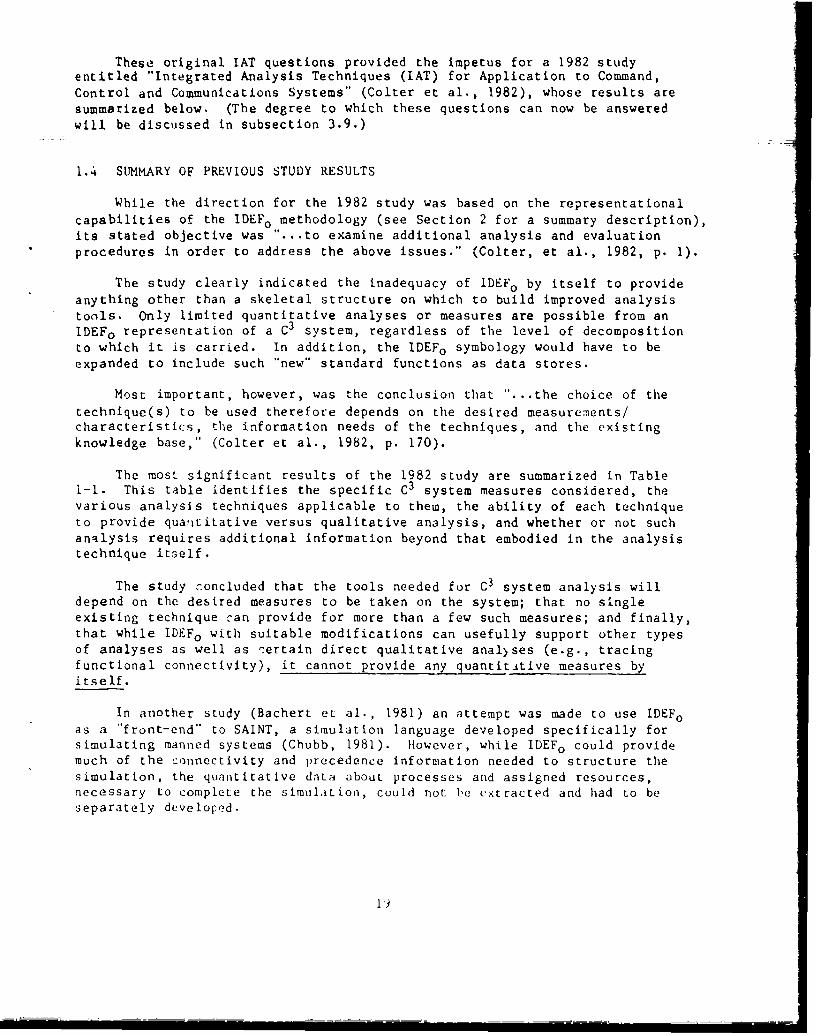
While the direction for the 1982 study was based on the representationalcapabilities of the IDEFo methodology (see Section 2 for a summary description),its stated objective was "...to examine additional analysis and evaluationprocedures in order to address the above issues." (Colter, et al., 1982, p. 1).
The study clearly indicated the inadequacy of IDEFo by itself to provideanything other than a skeletal structure on which to build improved analysistools. Only limited quantitative analyses or measures are possible from anIDEFo representation of a C3 system, regardless of the level of decompositionto which it is carried. In addition, the IDEFo symbology would have to beexpanded to include such "new" standard functions as data stores.
Most important, however, was the conclusion that " .. the choice of thetechnique(s) to be used therefore depends on the desired measurements/characteristics, the information needs of the techniques, and the existingknowledge base," (Colter et al., 1982, p. 170).
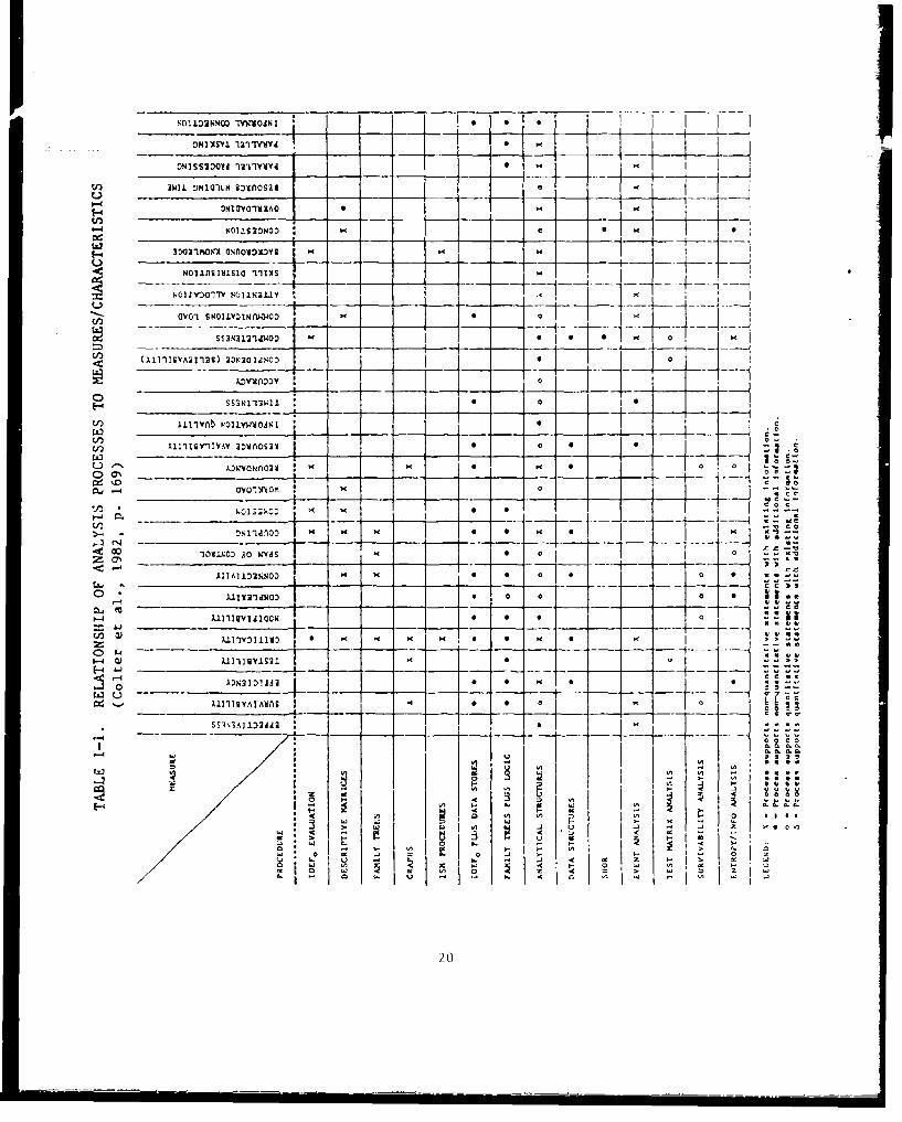
The most significant results of the 1982 study are summarized in Table1-I. This table identifies the specific C3 system measures considered, thevarious analysis techniques applicable to them, the ability of each techniqueto provide quaititative versus qualitative analysis, and whether or not suchanalysis requires additional information beyond that embodied in the analysistechnique itself.
The study noncluded that the tools needed for C3 system analysis willdepend on the desired measures to be taken on the system; that no singleexisting technique can provide for more than a few such measures; and finally,that while IDEFo with suitable modifications can usefully support other typesof analyses as well as :ertain direct qualitative analyses (e.g., tracingfunctional connectivity), it cannot provide any quantititive measures byitself.
In another study (Bachert et al., 1981) an attempt was made to use IDEFoas a "front-end" to SAINT, a simulation language developed specifically forsimulating manned systems (Chubb, 1981). However, while IDEFo could providemuch of the connectivity and precedence information needed to structure thesimulation, the quantitative data about processes and assigned resources,necessary to complete the simulation, could not be extracted and had to beseparately developed.
0.N1SS3001d 1n3vTd I
U) Iwil DNX o1U -,flSS t I I
_ _ _ _ __0' _ IIN11
SSNY N 1 1
___________ 1-40v- ON2yI~uoo
_-~~ c~iz_ _ _ _ _me,
SS)N~ 3 hI!:t -5 ~ -----. r13DNvv~b lOW dAo3
00 llglYY2tj OS21 so - - 0
z (71NA7 "
Iz -. Z~A1AIQI.)O . - - - Ia 0V
w 5 - t!~j - -
LVIII~tA'fli NS 20
In effect, then, we may conclude that at the outset of the present study,there was no single, existing, available Integrated Analysis Technique thatcould provide answers to all of the IAT questions listed in the precedingsubsection. Furthermore, there were no techniques available to meet theseneeds.
1.5 CURRENT STATUS
The work reported on in this report completes two of the four stages inIAT development. The first stage was the formulation of a static descriptionmethodology applicable to any system to be analyzed. The second stage was thedevelopment of quantitative techniques for estimating critical system perfor-mance parameters. The third stage, being initiated under separate subcon-tract, is to imbed the descriptive methodology developed to date in an easy-to-use job aid which will insure, to the extent possible, both completenessand consistency of system description and analysis. This will also provide a"1quick-look" capability for quantitative performance prediction at any givenlevel of system description or decomposition. The final stage will involvethe capability for analyzing the dynamic reconfigurability of a C3 system andthe allocation of resources to functions.
1.6 CONTENTS OF 'iS REPORT
The objective of this report, then, is to show how to describe a complexC3 system in such a manner that subsequent system analysis and performancequestions can be answered quantitatively. Our focus has been on how oneshould describe an existing system (as opposed to designing a new system),so as to capture the critical attributes of the system in ever-increasing(hierarchical) detail. However, we feel that the methodology will be equallyuseful in evaluating the design of new syst'-ms.
Section 2 of this volume summarizes the requirements for a static repre-sentation technique, while Section 3 describes the new hierarchical methodfor C3 system description and decomposition. Section 4 describes quantitativeanalytic tools for use with the static description. Finally, Section 5 pro-vides a summary of the results to date and a set of recommendations for com-pleting the development of Integrated Analysis Techniques for C3 systems, withspecial reference to the role of humans in these systems. Volume II of thisreport presents the results of separate applications of portions of the methodto a simulated system and two actual systems, and the lessons learned fromthese applicat it,1:,.
2]


SECTION 2
REQUIREMENTS FOR A HIERARCHICAL METHOD FOR STATIC SYSTEM DESCRIPTION
2.1 INTRODUCTION
The primary objective (and successful result) of IAT development since1982 was to find a single, self-consistent way to describe and model a complexC3 system in such a manner that manned system analysis and performance ques-tions could be answered quantitatively. The initial focus was on how oneshould describe an existing system (as opposed to designing a new system).The approach taken was to (1) capture the critical attributes of the systemin ever-increasing (hierarchical) detail and (2) overcome some of the majorproblems summarized in the 1982 study noted in the introduction.
In this section we summarize the requirements which must be met by astatic representation and modeling technique in order to be able to answer theIAT questions in Section I. These include the descriptive dimensions for C3systems; their decomposition requirements; the relationships among the dimen-sions; the types of system measures to be evaluated for a system; and the datamanagement requirements for IAT.
2.2 FOUR DIMENSIONS FOR DESCRIBING C3 SYSTEMS
For the simplest of systems, straightforward representations of physicalcomposition and connectivity such as system block diagrams, engineering draw-ings, "exploded" views, and "family trees" have long been generally acceptedtechniques. For more complex systems, so-called functional description tech-niques such as functional block diagrams (Goode and Machol, 1957) and DataFlow Diagrams (DFDs) (DeMarco, 1979) were developed as aids to diagnosing sys-tem failures and to designing new systems. Systems involving human operatorsand decisionmakers exhibited special requirements for representing informationflow, display, control and workplace design implications; and techniques suchas the Operational Sequence Diagram (OSD) were developed to meet these needs(Brooks, 1960).
With the advent of computer software, such process charts as data flowand operational sfquence diagrams evolved into the more or less standard meth-odology of the programming flow chart. However, as programs themselves becameincreasingly complex, new graphical representation techniques were developedfor the analysis and design of complex software systems. The StructuredAnalysis and Design Technique (SADT) is an example of such attempts at man-aging software complexity through "software engineering" (SOFTECH, 1978).
23

More recently, extension of these techniques to manufacturing systems andto information systems description has required that the physical resourcesneeded to support the various functions and processes be incorporated directlyinto the description (e.g., as in the Integrated Computer-Aided ManufacturingDefinition Language (IDEFo) as developed for the U.S. Air Force (SOFTECH, 1981).
However, when dealing with a complex, large-scale system such as a C3system consisting of a large collection of hardware and people performinghighly interrelated and interdependent functions, we find that organizational
-- issues and constraints transcend both the physical (resource) and functional(process) characteristics of such systems and must enter prominently into themethods for description and analysis. As an example, an Air Defense C3 system-will exhibit longer response times to attacking enemy aircraft if informationflow must follow strict hierarchical reporting paths than if the organizationpermits cross-telling of tracks. Classically, methods of organizational de-scription and analysis have evolved separately from (although they are often-confused with) those of process description and analysis. They include organ-ization charts which display lines of authority, responsibility, and coordi-nation as well as methods of representing organizational dynarmics (Beer, 1959;Berne, 1963).
Finally, while all systems are in some sense goal-driven, the most com-plex of these (including C3 systems) involve "organizations of organizations"of subsystems and people and are characterized by a complex, interrelated anddynamic hierarchy of goals which must be explicitly accounted for in systemdescription and analysis. Methods of goal decomposition and diagrammaticrepresentation have evolved for such complex, large-scale systems (Warfield,1973).
On the basis of problems encountered in applying earlier methods forsystem static description (e.g., IDEF 0 , OSDs, DFDs, etc.) and consideringthe unique requirements imposed by military C3 systems noted in the precedingsubsection, we conclude then that the following four distinct dimensions arerequired to describe such systems adequately at varying levels of detail:
& Resource (physical mechanism, human, geographic location, node)
* Process (function, procedure, algorithm)
* Organizational element (subdivision, unit, individual)
• Goal (intent, performance objective)
Finally (and of critical importance), the descrip '!e methods ultimatelydeveloped must be cable of generating important measures of system capability.
2.3 C3 SYSTEM DECOMPOSITION REQUIREMENTS
In the preceding subsection we defined the four dimensions along whichC3 systems must be described in order to capture their complexity as well as
24

their critical attributes. In this subsection we umaiethe requirenmertsfor system decomposition.
it is important to note that the very concept of decomposition impliesa hierarchical set of relationships within each of the four dimensions !.den-
~tified above. One of the major requirements of IAT is that it contains adescriptive methodology capable of representing not only the decompositionwithin but also the interrelations h ips among the four dimensions whl maifn-taininig concordance among the hierarchical levels of decomposition/detail.
Another critical requirement is that each dimension must undergo recursivedecomposition, starting at some initial or highest level of minimum detail.
* (The notion of a system bounda ry is Imp lied here, at least for purposes ofanalysis and/or desitgn.) The decomposition hierarchy can then be viewed asa "tree," with the "trunik" represenLing the highest level and the "branches"constituting each Succeeding level of greater detail. For analysis purposes,we cef ine the "leaf" level as the point at which the decomposition Is tertia-nated and a model is used for thle process representation. The model parametersand characterisWtics are then determined by the requirements and constraintsset by the physical 'resource and orA~ni zatýIio entities and by the goak hier-archy to which tile system is responding.
The LAT riethodology requires that at aLQX decomposition level, raodels mustbe capable of being defined and exercised in order to be able to estimate sys-tem performance and effectiverness. At the higher levels (less detail) thesemodels must, of necessity, be extremely aggregated. This is well reflected inPaSL aLLtwp18j to rtep.ebenL entire C3 systems by sitaple time delays. However,
th rql emn frrecursive deojs.to en htthe mode inj methodmu'it ~ienticall~y a~licbea ahlevel of dýcoM~sLwiL.rth oH 1n tie amount of detail and the prmtrvalues ch Lnj between
l evelsa. Thus, sel ect~ion of Ith most appropriate models and definition oftheýr Interdimensiocal relationships (as, for example the effect of a given
resorceon the Lri:cess that It supports) has been a major requirement forsuccessful IATr development.
In the following subsections we defi ne in further detail the four decomn-position dimeosionis and the manner by which successive levels of eletail Mubtevolve. Note that the ability to decouipose a systew along _pýV of itr dimen-sions separatelv will be essential for C3 systemas analysis and synthesi_--.
2.3.1 Process; DevoiVoS~itiull
Includeud 'n hie process dfmension amre Such things as functions, processes,procedures, prutroo>, ana scri pts. Thl~s dimienslon has long been recognizedand us'ed IS L1 thu. ost salitlent diffiesllo4n for decotapositton , and has receivedthe greatest; attlmntutn in earliur efforts (SOFrLFCl, 1981). The hierarchicalori!ar,1zat;.1 (.! I C3 ;vcmtý:, that is, its s~ibdiv~sion into subsystems (e.g.,survel i anc , --4eIpol Cec~rol , e.)is dl ret I y reflected fii process decom-
f')tlu ~b iat4
il' reliurred to !ý .SLTcuI uruuuiziL fuon Or LeVen SyStem~

structure, in this report we will use the term "process decomposition" through-out, since "organization" usually refers to the representation of authority,responsibility and coordination; while "structure" refers to the functionconnectivity among system resources. (See further discussion of these termsin subsection 2.3.3 below.)
Thus, the primary decomposition of a process pl at a level L0O involvesspecifying the following:
1. What higher-level process pL-1 It is a a~rt_ of; and
2. What lower-level processes [pL+l] it consists of.
It is also necessary to specify its functional connectivitles, that is, tospecify from which processes at the same level a given process receives inputs,as well as to which other processes it provides outputs.
2.3.2 Resource Decomposition
Included in the resource dimension are the physical resources, equip-ments, nodes, locations, and physical zonnectivities which support or carryout the processes. The resources of the system include both its physicalfacilities and hardware (including imbedded computers and associated software)ab well as its human operators and decisionmakers.
The decomposition of a resource into its component parts is usually well-defined from the standpoint of its physical composition. Thus a resource RL
at level L>O (e.g., an aircraft) is part of a larger resource RLI (e.g., asquadron) and itself consists of a set of subresources or components {RL+l}
(e.g., its engine, avionics, etc.) at level L+l. We make the followingassumptions:
Al. Resource decomposition is nonoverlapping, i.e.,
RLI fr RLJ - 0 , *j
Physically, this means that if RLi is removed (from RL-),the RL4 ifj remain iliLact (even though they may not function).And, of course, since the sum of the parts equals the whole,
A2. A human resource is nondecomposable*. Hence, If
*In some previous work, various human attributes have been defined as sepa-
rately available (sub)resources. However, we believe this to be erroneous.While an individual can perform several tasks in an apparently siuiultaneousmanner, it is clear that the apparent simultaneity is really the result of"chunking" of data, efficient time-sharing among the several tasks, ar,dwell-traIned response organizations. We will assume that the human, as anoperator or declsionmaker, is only capable of acting as a serial processor.
26

UL RL is a person, then RLi+l = RLi
A3. In the case of computers, we will assume that the hardwarememory elements, disks, etc. are resources. However, theprograms can be either processes or resources, dependingon the application (e.g., imbedded computers, which are partof a fire control system, use programs that are part of"the imbedded computer resources).
In a few instances, the decomposition of a resource can benon-unique, as for example when there is no a priori logicalway to group the parts that comprise the whole. To minimize
non-uniqueness, we establish a linkage between resource andprocess decomposition by assuming that:
A4. The subresources {RL+li} at level L+l must be those that areassigned to support or carry out the subprocesses [pL+lj} atthe same level of decomposition.
In existing systems, it is usually the case that resourcesand processes are more or less directly related (in the sensethat specific resources were selected to support specificprocesses); thus assumption A4 will generally be satisfied.However, it is important to recognize the fact that while agiven resource is assigned to support only one process, itmay be capable of supporting several. The notions of flexi-bility and adaptability derive in large part from the abilityof organizational elements in a C' system to reassign respon-sibilities among lower-level organizational elements and toreassign resources to support other processes, as will bediscussed below.
2.3.3 Organizational Decomposition
The military organization provides the fundamental control mechanismswhereby humans and machines work to attain objectives. Decision authority,responsibility, coordination and goal-setting are the primary attributes asso-ciated with organizational elements; they allow decisionmakers to reassignresources, processes, and organizational elements and to modify objectivesif necessary, in order to adapt to a variety of changing circumstances in themilitary environment.
Of course, all C3 systems will evolve and change as they take advantageof new technology and as they are called upon to support new or changing mis-sions (e.g., search and rescue). Also, one may be interested in questionsrelating to off-nominal performance such as system survivability, adaptability,and flexibility (e.g., due to loss of a resource, failure to meet an objec-tive, etc.). In either case, one must include organizational representationin system description.
27

The primary decomposition of an organizational element 0L defines thelines of decision authority (i.e., command structure and accountability, orreporting-to), responsibility (i.e., control), and coordination. With respectto authority, element 0L at level L is only accountable to a single element0 L-l at a higher level and has authority over the set of elements {OL+lJ atthe next lower level L+I, which in turn are accountable to OL. This authoritydecomposition defines an organizational hierarchy.
With respect to responsibility, the relationships are more complex.Organizational elements have responsibility for the processes and resourcesassigned to them, and authority over lower-level elements; and they areaccountable to higher-level elements, in strict accordance with the lines ofauthority described above. Note that a human being is a resource which canfulfill various organizational requirements at different times and to dif-ferent purposes or goals. Thus, there may be instances in which a lower-levelelement is accountable to one higher-level element for one set of processesand/or resources and to a. different element for another set. Such accounta-bility to different "bosses" for different activities characterizes theso-called matrix organization, and is exemplified by the "multi-hattedness"of many U.S. military commands. This can be quite different for non-U.S.commands.
Note also that an organizational element has responsibility for control-ling processes, and that these processes can include reassignments of lower-level decision authority, i.e., of accountability and control.
Finally, from a decomposition standpoint it is important to recognizethat an organizational element at level L may be responsible for two funda-mentally different classes of processes:
1. those at the same level L that directly support the functionsof the organizational element in question; and
2. those at the next lower organizational level L+I into whichthe function at level L decomposes.
Classically, these are known as "staff" and "line functions," respectively.
As noted earlier, it is extremely important to distinguish betweenorganizational and process decomposition. Among systems engineers the term"organization" is usually taken to refer to the way in which the system itselfis hierarchically and/or functionally organized (i.e., structured or decom-posed), whereas among human factors specialists, the very same term is usedto represent the lines of authority, responsibility and coordination amongthe personnel in the system. For example, from an engineering standpoint, aC3 system is generally "organized" into a surveillance subsystem, a planningsubsystem, a controlling subsystem, an order dissemination subsystem, a commu-nications subsystem, etc. On the other hand, the structure of the system isusually taken to refer to the functional connectivity among the resources ofthe system, that is, which processes must "talk to" or coordinate with whichother processes, and which resources must bc connected to each other in orderto provide for the required data flow among the processes.
28
In this report we shall use the following definitions of these terms:
0 Process decomposition: hierarchical subdivision of processesinto their component subprocesses. Results in multiple levelsof description at successively finer detail.
"* Resource decomposition: hierarchical subdivision of resourcesinto their component parts. Also results in multiple levelsof description at successively finer detail.
"* Organization, or organizational decokiposition: hierarchicalsubdivision of decision authority, responsibility, and coor-dination among all system processes and.or resources (includinghumans as resources).
* Structure: connectivity among 311 system processes and/orresources (including humans as resources), at a given levelof decomposition or description.
In some cases, as we shall see, the very existence of connectivitybetween two resources implies either authority (as for example in a prece-dence relationship such as "A before B") or coordination (as for example ina joint presence relationship such as "A and B before C"). However, the con-cept of responsibility is peculiarly huan in that it can only be offered(to be either accepted or rejected by an individual) but never delegated:whereas authority can indeed be delegated. On the other hand, authority andcoordination can always be "wired in" to a system by design, but hardware orsoftware parts of the system cannot take responsibility for their performance.This is especially important from a human factors standpoint, since the systemmust be carefully designed to support the human roles (i.e., their authority,responsibility and coordination needs) in the system.
2.3.4 Goal Decomposition
Goals are established by organizational elements and must therefore beincluded in parallel with the organizational dimension. In fact, the estab-lishment of goals, resolution of conflicting goals, partitioning of goals intosubgoals, and assignment of responsible organizational elements to achievethese subgoals are perhaps the most important of all organizational activities(i.e., management).
The fact that an individLu.l can and does act both as an organizationalelement and as a resource can be a major source of confusion unless it isrecognized that:
0 an organizational element sets goal,; for lower-level elements.This is based on the effectiveness re~uirements placed onlevel 0 L by the next higher level ,)L-,;
29

0 these goals are equivalent to performance requirements for theprocesses pL+1 at level L+l for which OL+1 has responsibility(i.e., is assigned);
* the processes pL+li are supported by resources R1+1 at levelL+I. The degree to which a goal GL+l is met is determined bythe degree to which the resources RL+1 assigned to that process ..can meet the process performance requirements implied by thegoal;
the goal becomes the means by which the entire C 3 entity(process, supporting resources, and responsible organizationalelement) is controlled.
Figure 2-1 summarizes the intera:tlons among the C 3 dimensions and demonstrateshow goals are used in controlling both processes, resources, and organizationOnly line relationships are shown i-a order to simplify the diagram; staff ele-ments would be shown as L-level processes and resources that directly supportthe line functions at that level.
2.3.5 Relationships Among Processes , Resources, Organizational Elements,and Goals
Frow Fig. 2-1 it is clear that a C3 system exhibits several classesof interactions. In this section we examine the most important of theseInteractions.
In general, a process requires inputs and provides outputs. The result-ing information flow among processes is only an indirect determinant of systemtopology (i.e., it only implies connectivity); however, in reality, informa-tion exchange takes place not among processes but among the physical resourcesthat support and are assigned to the processes. If connectivity between twoC 3 resources is broken (e.g., a radio link is jammed), then the informationflow between the processes supported by these resources (e.g., Intelligenceinformation) is halted. We therefore -incorporate system topology in resourcedecomposition by defining at level 1. the resource connectivity matrix,[RL4 .x Rtj];
SRLL4 1 R I If resource RL4 sends !nformation to resource RL
i =
0 otherwise
Thus, the nonzero elements of the i-th row of [RL 4 x RLj] indicate those re-sources to which RL; sends information, and the nonzero elements of the i-thcolumn ofT-R-i x RLj] indicate those reso:rces from which 1L-1 receives infor-mat'on. Note that the nature of :onnectivity implIes that for every nonzero[RLW x RLi], there should be at least one nonzero element of xRL+Iz - RL+]correspon•ing to the connectivity between the decomposed elements of RL;and RLj.
30

DIMENSIONS
LEVELS GOAL ORGANIZATION PROCESS RESOURCE
HIGHER L-1 GL- 1 U1
/ N -
L / L 0
wi
\ ,
LOWER L+I GL/ oI 0 .RL+
pLJ
LEGEND(t {) where I ranges over all elements at level 1.
xA i-th element of X at level 1.
ASSIGNMENT An organizational element (0 1 at a given level (L)(from level 1) establishes goals for the next lower level (L+I); 01
(e.g.. a commander) assigns goals (GL+), processes (pL+l).resources (RL+). and organizational elements (0L+1)
(e.g.. subordinates) to meet these goals.
ASSIGNMENT OL has been assigned goals (GL). processes (PL). and(from level L-1) resources (RL) from organizational elements at the next
higher level (oL-I).
RlSPONSIBILIiY ixercise of responsibility within a level for
meeting assigned goals. R-23070
Figure 2-1. Recursive Nature of Decomposition
31
In addition, for each nonzero RLi x RLj], there should be a correspondingspecification of the nature o.- the Interconnection (e.g., telephone, micro-wave), the attributes of the interconnectioa (e.g., throughput), and a speci-fication of the type of information transmitted. Of course, the higher one Jis in the decomposition (smaller L), the more general and all encompassinga----re the information flow descriptors.*
It is also possible to include input-output connectivity in processdescription. This serves to express what is required for process input andoutput, as opposed to what is actually available, and any inconsistency betweenit and the resource connectivity matrix can serve as an "error signal" andstimulus to an organizational element for resource reassignment. In a manneranalogous to the resource connectivity matrix, we define at level 1. the infor-mation flow iequiremerits matrix, or process connectivity matrix, [pLi x pLj];
[pLi x pL j] 1 if resource PLi requires information from process pL
0 otherwise
Again, supplementary data about the information required for each nonzeroelement of P should be provided.
Finally, in a similar vein, we can represent coordination among organi-zational elements at the same level via the coordination matrix at level k,OCk:
o o~ = 1 if resource 0o-i coordinates with oLj
0 otherwise
where, again, supplementary data about the nature of the coordination mustalso be given.
Note that since the dual of any square matrix is a graph, the foregoingmatrices can be used directly to generate resources connectivity trees, pro-cess information flow diagrams, and organization charts.
2.3.6 Cross-Referencing and Redundancy Requirements: Assignment andAssignability Matrices
If each of the four dimensions were decomposed separately, it would bevirtually impossible to maintain consistency across the dimensions at any
*Note that in the 'manner analogous to "indirect addressing" in computer sys-teins, the location where supplemental information data are stored could beused instead of a "I" in [RLi • Rj.
32

given level of detail. However, tying the decompositions together providesthe basis for a consistent, balanced, and cross-referenced system description
methodology. This was a major requirement for IAT development.
... +-Thus, at any level L in the decomposition, it is necessary that:
I. A process description contains references to the resources
required for its performance, as well as references to the
organizational element responsible for monitoring and/or
controlling the process and to the goal (i.e., performance
requirement) that the process must meet. Finally, it contains
references to the input and output functional dependencies
between itself and those other processes at the same level
with which it is directly related.
2. A resour!,ze description contains references to the process(es)
which that resource is assigned to support, as well as ref-
erences to the organizational element responsible for t ae
resource. It also contains references to the physical con-
nectivities between itself and those other resources at thesame level required to support a specific process.
3. The description of an organizational element contains refer-
ences to the processes that the element is responsible for
monitoring and/or controlling, as well as references to the
resources which are assigned to that element and to the goal(s)
for which it is responsible. It also contains references to
the lines of authority, responsibility and coordination
between itself and those other organizational elements both
at the same and other levels as required to attain a specificgoal.
4. A goal description contains references to the organizational
element responsible for the attainment of that goal as well as
the process(es) for which that goal is a performance require-ment. It also contains references to the higher-level goals
of which it is a part, as well as to the lower-level goals
which must be met in the interests of its own attainmetnt.
This cross-referencing is accomplished by means of assignment matrices.
Thus, at any level L, any of the four dimensions can be described by a coin-posite vector (matrix) of four parts:
I Pl. x RL x 0L x GL]
with its primary decomposition (e.g. , pL, as in Fig. 2--2) and three cross-
references (e.g. , Rl, OT- and GI-). Once again, Lhuc redundancy inherent in the
cross-references over four dimensions can serve as a check on consistency of
tlhe data that define the C3 system as wcll as a means for detecting errors
33

in specifications. Another reason for such cross-referening is to force, tothe extent possible, a logical consistency and balance among the four dimen-
sions. Cross-referencing can help to insure that the four decompositionsproceed in parallel, as opposed to reaching extreme depth in only one or two.
pL i
pl,+lj(j- to 4) pL+1l pL+1 2 pL+1 3 pL+l 4
Figure 2-2. Example of Primary Process Decomposition
The various relationships described above can conveniently be representedin matrix notation as shown in Table 2-1, which presents a three-letter mne-monic descriptor, a brief definition, and a symbolic representation for eachrelationship.
it is worthwhile to examine in somewha.t more detail the nature of thespecific assignment matrices. The matrices [OxG] and [OxP] at level L, whicheffectively assign responsibility for goals and processes to organizationalelements are the subject of original system design and/or long-range planningin any C• system. On a somewhat shorter time frame, the matrix [O×R] at levelL reflects the issues of resource responsibility (sometimes referred to as
"ownership") and is a major focus of system reorganization and reconstitutionin battle. This depends heavily upon the concept of assignability, which willbe defined next.
Note that decomposition along any dimension can also be represented inmatrix form. For example, the matrix [OL x OL+I] represents the organiza-tional decomposition (i.e., organization chart) or lines of authority in thesystem while the matrix [OLix oLj] represents the chart of human coordinationin the system within a decomposition level. Similarly, the matrix [pL . pL+l]represents the process decomposition in the system while the matrix [pLi . pLj]represents the coordination or connectivity among processes within a decompo-sition level.
Finally, in order adequately to represenlt the inherent adaptabilityresulting from the capability for reassignment of resources, goals, processesand even organizational elements in a C3 system, we must define a set ofassignability matrices [.1*. For example, the matrix [R×PI* at level L mustshow which resources are capable of sukporting (i.e., are assignable to) eachprocess. Assignability matrices [O×G] , and [OxR]* can also be used to rep-resent the capability of various organizational elements at a given level to
34

TABLE 2-1. RELATIONSHIPS AMONG THE FOUR DIMENSIONS
REPRESENTATION
DESCRIPTOR DEFINITION RESOURCE PROCESS ORG'L EL'T GOAL
ISA Is known as (name) (name) (name) (name)
AKA Also known as (name) (name) (name) (name)
POF Parts of RLi e RL-lI pLi C pL-1 0Li C oL-1I GLi c GL-j
COF Consists of RLi = {RL+1j} pL= {pL+l } oLi = oL+j} GL4 = {GL+lj}
STO Sends to; [RLi x RLj] [pLi x pLj] [oLi x oLJ]
connects to;informs; coor-dinates with
RFM Receives from; [RLb x RLJ] [pLj x pLi] [oLi x 0 L 4 ]
is connectedto; is informedby; Is coor-dinated with
ATO Assigned to [RLb x pLj] [pLi x oLj] [oL-li x oLj] [GLi x pLj
[RLm x 0Loj [GL; x oLj]
AST Assignable to jRLi , oLj]* [pLi x oLj]* [oL-li x oLj]* [GL 4 x pLj]*
[RL , x o--]- [GL 4 x oLj]*
Notes:
1. Superscript = level of decomposition
2. Subscript = inde,:
3. Read RLi as "i-th resource at 'evel L"
4. Read [AxB] as A "sends to, etc; receives frou, etc; or is assigned to" B
5. Read [A×B]* as "A is assignable to B"
35

take responsibility for various goals, processes, and resources at the samelevel. An assignability matrix ultimately should contain as its elements(cells) an assignablit_ ilnde x, i.e., a numerical quantity representing therelative capability of a given resource (including humans) to support a givenprocess; or the relative capability of a given organizational element to takeresponsibility for a given process or resource (e.g., as a function of training,experience, or workload).
It is important to note that an assignment matrix (e.g., [RxP]) differscompletely from its related assignabillty matrix (e.g., [RxP]*) in that it ismuch more sparse; of the many things a given resource could do, it is onlyAedignqý to do a small subset (perhaps only one) of th-em. -- If all resourcesare "dedicated" to single processes, then a square, diagonal assignment matrixresults and the resource is subject only to queuing delays due to workload.On the other hand, if a given resource is assigned to support two or more pro-cesses (as is typical with both humans and computers), it is then a sharedresource and is subject to contention, as well as queuing delays.
Note that if we assume a fixed organizational structure with fixedgoals, as would be typical of a "mature" C3 system, then the actualon-line modification of such resource assignments in [OxR] and/or[RxP] within the constraints of [OxR]* and [RxP]* constitutes thesystem's adaptive capability vis-a-vis attaining its goals withits available resources. A more flexible arrangement would permiton-line reassignment of goals among organizational elements [OxG]within the constraints of [OxG]*, as an additional adaptivecapability.
The requirements for combining process, resource, organizational, andgoal decomposition as described in the preceding subsections provides a farmore powerful tool than, for example, an IDEFo description, which at best iscapable only of process decomposition with an attached indication of associ-ated resource and "control" requirements, and no capability for representingeither actual resource connectivity or organizational authority, responsi-bility, or coordination.
2.3.7 Depth of Decomosition
A major issue in any decomposition methodology is how to decide whereand when to stop decomposing. While gross allocations of resources (includinghumans) among processes can often be made at higher decomposition levels usingsimple connectivity and aggregate performance data, the decomposition gener-ally should be carried out to one level below that at which the user seeksthe answers to specific questions. The decomposition ends at that level, withcareful attention paid to: (1) the interactions among the Lirocess performancemodels (based on the assigned resources) representing the descriptions at thislevel and (2) the model. parameter data, as opposed to carrying out any furtherdecomposition. We shall return to this point later when describing theselected modeling technique.
36

2.4 DATA STRUCTURES FOR IAT
While the matrix notation described above assists in organizing one's
thinking about the relationships among the descriptive data about a C3 system,-we also need a means of organizing the data itself to capture these relation-
ships. Nearly any flexible, well-structured database management approach canprovide such a capability. However, the use of frame/slot notation, a tech-nique borrowed from artificial intelligence, is particularly advantageous.
Frames were originally proposed by M. Minsky as data structures forreprest.nting knowledge of stereotyped situations, such as being in well-knownenvironments (e.g., one's living room, office, control room facility) or goingto special events. Frames served as components of a broader theory of humanmemory and performance in their role as "units of recall," in Minsky's origi-nal conception: frames were selected from memory whenever one encountered anew situation, or made substantial changes to viewing current conditions orproblems at hand. It is in this sense that frames received more widespreadapplication as templates, i.e., "... remembered framework(s) to be adpated tofit reality by changing details as necessary" (Minsky, 1975).
Although Minsky intended frames to be employed in conjunction with asso-ciated types of information (viz., how to use a particular frame, expecta-tions about what will happen next, what to do if these expectations are notconfirmed), the use of frames within artificial intelligence (Al) modelinghas focused more on the internal structural properties of frames as aids fororganizing data (Schank and Abelson, 1977; Barr and Feigenbaum, 1981).
To be viewed as data structures, frames can be conceptualized as networksof node-, and relations. (Note the correspondence of this concept with two ofthe7O descriptive dimensions: resources and processes.) The top levels ofa frame, in this context, are fixed, and represent conditions that are assumedto be true about a specific situation. The lower levels nave terniinal rodes,called slots, which are syntactically "place-holders" -- slots must be filledby particular instances or data values. Each slot can be used to specify con-ditions that its assignments must Meet. Simple conditions are specified bymarkers that might require a terminal assignment to be a person, an object ofsufficient valuer,, or a pointer to data associated with another s-it or anotherframe. More couplex conditions can specify relations among data assigned toseveral slot:o (Minsky, 1975). Collections of semantically-related frames canbe linked together into "frame-systems." Different frames of such systemsshare the same terminals: thi:; is the critical point that makes it possibleto coordinate information gathered from different vievpoints. Differencesbetween the frames of d-i system can thus be used to represent actions, cause-effect relatLions, or changes in vantage points (e.g., from which the same dataare perceived or precessed).
Another importait ;iSpect of frames lies In the default values of slots.Default jssiinments can bLh used to expre-ss prototypical, potent ial, or accept-a Lio va •,ie;. elieice,, through default values., iranes can be used to representgc'•L'ric informatlon, CXpCjctLaions, and the like (Yager, 1984).
37

Default values have further uses within frame-systems. In particular,prototypical or "normally expected" values can be vsed to test the validityof a frame, in cases where some slots are filled in with acceptable valuesat the same time other slots have not (yet) been g!v.n assignments. Slotsalready filled-in can be used to predict the -alues of slots whose assignments-are lacking. This feature of frame/slot notation makes these data structuresespecially helpful toanalsts who must collect field data known to beincomplete.
For application to IAT, frames cinstitute major data sets for each ofthe four dimensions: GOALS, ORGANIZATIONS, PROCESSES, RESOURCES. "Slots"describe the data elements of a frame.
The advantages of using fraines and slots ire as follows:
I. Relationships that might be captured in several differentmatrices can be grouped together on a single frame.
2. Slots can be used with and without entrieq to Indicate whetherperformance data are or are not available.
3. Default values can be defined in slots for carrying out sensi-tivity analyses and "zero-order" estimates of performance.
4. Cross-referencing can be handled by supplying pointers fromframe-to-frame (indicated as entries on slots).
5. Slots can be added or deleted to specity attributes of thedynamic characteristics of a process.
6. The inherent nesting properties of frame and slot notationmake it possible to capture inforuation from structuralmodels (recursive decompositions and matrices in TAT).
Figure 2-3 illustrates frame and slot notation.
2.5 C3 SYSTEM MEASUKES
We now turn to a major problt faced by C3 systems analysts and engineersin the past. Thece has been a serioud divergence of opinion between militaryoperations personnel and systems designers and analysts regarding how to mea-sure the utility of these systems. Military personnel lean toward measuringphysical quantities (or their equivalent in computer sifnulatioas) whichdirectly affect a battle outcome, such as "bombs on target," assigned targetsdestroyed," "attrition rates," ctc. Engineers, on the other hand, tend tothink in terms of the capabilitLie of the subsystems and systems they aredesigning or analyzing. As a result, some confJsion hags deLveloped with regardto the meaning of various typesm of measures.
I 8

LEVELS MISSILE WARNING OFFICER /COMMAND WARNING CENTER(MAO) ROLE / (LWC)
MWO CONSOLE:
HIGHER L O• A SUSPECTED Gi R STAFF ASSIGNED. .. ATTACK TOPL MODTE
ij MONITOR FOR ENEMYSMISSILE LAUNCH
TO TRANSMIT IMWO CONSOLELoWER L41 NT TREPORT G 1 R L+1 STAFF ASSIGNED
EvENT REPORTS ACTING DUTY TO ADO DUTIES
OFFICER (ADO) 1 N D E
<ROLE> ACKNOWLEDGE MESSAGE
I +16l ASSIGN EVENT NUMBER
3 GENERATE EVENT REPORTS
-Z2313A
PROCESS NAKE: MONITOR FOR ENEKY MISSILE LAUNCH
GOAL: TO ADVISE CDC OF A SUSPECTED ATTACK
ORGANIZATLONAL ELEMENT: MISSILE WARNING OFFICER (lNO) ... primary responlbilityACTING DUTY OFFICER (ADO) ... delegated responsibility
PARENT PROCESS:
SUB-PROCESSES REQUIRED: 1) ACKNOWLEDGE KESSAGE2) ASSIGN EVENT NUER3) GENERATE EVENT REPORTS
IN. JTS REQUIKED: MESSAGES - (4 TYPES)
1) INTELLIGENCE2) SYSTEM STATUS3) ADS4) ass
OUTPIUTS; eVENT REPORTS - (3)
1) AD512) ADS23) as5
HEASULK, OF" I'FRkFORLhACE; TIMELINESS
ACCUKACY
RESOURCES KEQULIkrD: MWO CONSOIESTAFF ASSIGNE) TO KfJ3/ADO DUTIES
ILgure 2-3. Exa:,ple of IAT Structural De.;cription and Process Frame for the
' iucess " onttor for Enemy Missile IitLnch" (Kornfeld, 1984)
59

To clarify the situation, we define the following six fundamental typesof measures associated with C3 systems:
1. System capability measures describe what a C 3 systems (or, moreproperly, what the system components or physical resources)can do (e.g., radar peak power, communication channel bandwidthor capacity, human cognitive and workload limitations, computermemory size, display resolution, and other attributes). All ofthese measures can be evaluated based on physical properties ofhardware or human elements of a C 3 system, without reference toany ilitary or natural environment. Capability measures arespecific to C3 resources and represent one class of !ndejendentvariables, namely, the desijnvariables of the ststem w~th
whfch engineers can deal more or less directly.
2. Mission environment measures describe the situation whichdrives the CT system, i.e., those factors which consitute thethreat to and the environment of the system (e.g., radar crosssection of an aircraft; reflectivity and absorbance of theatmosphere; number of hostile emitters in a region; hardnessof a target; flyout time of a missile). All of these measurescan be determined from the military situation and environaentin which a system is or might be deployed, without referenceto any specific C3 equipment or physical resources. Missionenvironment measures represent a second class of ýnde ndentvariables over which, however, neither military nor engineeringpersonnel have any direct control.
3. Syste erformance measures describe what the C3 system itself(or, more properly, specific C3 functions or processes) willdo when driven by a specific threat and environment (detectionrange for a radar; access time to a computer memory; messagequeue lengths for a comunications service; time required toassign a weapon to a newly detected target). All of thesemeasures can be evaluated only if characteristics of both thesituation and the C 3 system are known, since they depend on hw-the sjstea drives and is driven by its environment. Perfor-mance measures are dependent variables and are specifLc to C3
proc e ss es .
4. Xilitaryeffectiveness measures descr!be what the combinedeffects of thGervstemand thewe aoJn _ystems which it con-trols will be when driven by a specific threat and environment(probability that a hostile missile !s destroyed before itreaches its target; attr!.:-on rates; fraction of attackers suc-cessfully penetrating fr endly dtefenses; fraction of attackerssuccessfully engaged before reaching target; movemenz of ForwardEdge of Battle Area). All of these measures can be evaluatedonly with respect to criterion levels set by military conmanderson the scene. Effectiveness measnres also are dýeendent
•0

variables but are specific to military jpals and of necessitymust take into account weapon system as well as C 3 systemperformance. As an example, "number of weapons hitting desig-nated targets" as a measure depends not only on weapon deliv-ery system accuracy but also on target detection, recognition,countermeasures effectiveness, and other C3 system performancecharacteristics.
5. System survivability measures describe the ability of the C3
system to continue to perform one or a group of necessary pro-cesses or functions in the face of enemy attack on the systemItself. For example, such a measure may be the probabilitythat the surveillance subsystem will continue to provide atleast 90 percent coverage of a specified spatial volume duringthe time period of the attack, with less than 5 percent downtime. Similar measures may be defined for other subsystemssuch as communications, planning, and weapon direction andgenerally will be stated in terms of probabilities, times,spatial boundaries, etc. Survivability will be determinedby such things as: (I) communication, or connectivity amongresources In the system; (2) redundancy of dispersed resources(i.e., number of "copies" of individual resources physicallylocated in different geographical areas); and (3) the reassign-ability of resources to perform different processes as wasdiscussed in detail in subsection 2.3.6).
6. System efficieney measures describe the way in which availableC system-resources are utilized. A highly efficient systemrequires a minimum of resources to do its job; thus, resourceutilization in such a system should be very high. However, itis important to recognize that one cannot have both high effi-ciency and high survivabilicy at the same time in the samesystem. Since, as noted in item (5) above, survivability isachieved via geographically dispersed multiple copies (i.e.,redundancy) of resources, then resource utilization and henceefficiency must necessarily be low in a highly survivablesysrem.
Note that it may not be feasible to improve a system design with respectto effectiveness, efficiency and survivability slmultaneousl•y. However, giventhe development of appropriate mathematical tools, it should be possible tomodify a system de!Ign in order to:
0 Irymprovu effectiveness subject to minimurm constraints on surviv-ability and efficiency; or
0 Improve efficiency subject to ininimurm constraints on surviva-bility and effectiveness; or
* Inprove survivability subject to uinfinmim constraints on effec-tiveness and efficiency.
41

Such tools would make it possible to determine whether one or another of theconstraints must be "broken" and by how much, in order to reach a given levelof improvement (i.e., it may tur. out that a slightly lower effectivenesscan result in a major improvement in survivability for a given level of effi-ciency; or that a small decrease in efficiency can result In a major improve-ment in effectiveness, etc.). The trade-off possibilities simply cannot beignored.
It is especially important to distinguish clearly between these types ofmeasures when attempting to evaluate and/or predict human performance in thesesystems and its impact on system performance and effectiveness.
2.6 POSSIBLE APPROACHES
The definition and evaluation of C3 system measures can be supported inthree different ways (in increasing order of difficulty and expense, but indecreasing order of validity): by analysis, modeling and simulation, andexperiment. Analytical techniques include PERT/CPM, queuing network theory,and related methods. These methods are primarily limited regarding the size(i.e., depth of decomposition) of the systems that they are able to represent.Modeling and simulation techniques include the use of such standard languagesas SLAM, SAINT, and CSMP as well as more elemental methods such as Petri netmodeling.
In this section we have reviewed the primary requirements and constraintsfor C3 system description, decomposition, measurement, and data representa-tion. Because bf its generalizability and wide applicability as well as itsdirect capability for decomposition, we have selected an extension of thePetri net methodology for further development. In the following section weshall describe a Petri net modeling and simulation toethodology that meetsthese requirements and at the same time allows us to define the significantsystem measures and extract both structural and quantitative measures.
42

SECTION 3
STAPNs: A FORMAL MODELING AND ANALYSIS METHOD FOR IAT
3.1 INTRODUCTION
In Section I we noted the differences between C3 Systems and other large-
scale systems. These differences comprise one major reason for the difficulty
experienced in attempting to analyze C3 systems. A second major reason has
been the lack of a complete, well-structured intellectual framework which can
capture all essential elements of C3 processes, resources, and organizations.
More useful analyses should be possible if we can (I) create a formal analysis
framework for describing C3 systems which meets the requirements set forth inSection 2; (2) use that framework to identify a precise, inde endent, and com-plete set of variables or measures with which to describe a Cý system's beha-vior; (3) use the same framework to) develop quantitative relations among thevariables; (4) deduce numerical values for each of the variables using empir-ical or theoretical data; and (5) use the same framework for representing andanalyzing both human and system activities.
This section describes ALPHATECH's approach to meeting these requirements.it is based largely on recent work by Tenney (1986) and Blitz et al. (1985).We first summarize the minimum set of physical constructs required for C3 sys-tem modeling. This is followed by a short tutorial on the technical foundation(i.e., mathematical constructs) underlying the methodology, namely, Stochastic,Timed, Attributed, Petri Nets (STAPNs). The reader will note that the formalstructure of STAPNs is directly analogous to the empirical structure of C3 sys-
tems; it is this analogy which forms the basis of our approach.
*We then introduce the concept ot the -box node,- a new Petri net primi-tive. Next we describe the tight relationships between the physical attri-butes of a C3 system and the mithemr.itical modeling formalism of STAPNs.
Finally, in the remainder of is section we discuss four additionaltopics:
* Relationship of STAPN's to -xisting -_-t.thods of system represen-tation, modeling and analysýis
* Guidelines for constructit'- IAT process models with Petri nets
S zHowu STAPNs can be used to model hurnan operator and decision-n-wa king activities
* Which IAT questions mnay nrm- be addressed and which requirefurtnther IAT develop;-nent
43

Details of the methodology are presented in Appendix A which describes(1) the canonical performance measures which are directly derived from theSTAPNs; (2) the formal method of model refinement via model decompositionand enhancement; (3) relationships among the measures at different levelsof decomposition; (4) available techniques for evaluating the measures; and(5) open issues, i.e., problems which have not yet been solved. Subsection3.8 contains procedures and guidelines for generating measures from STAPNs.
3.2 PHYSICAL CONSTRUCTS FOR C 3 SYSTEM MODELING
The descriptors of C3 system behavior must relate to reality. For thesake of measurability and, ultimately, of performance evaluation, they uustbe tied to physical activities in specific, concrete ways. The approach de-scribed here injects an abstract representation between reality and the mea-sures, and that representation must be closely tied to reality if the impliedmeasures are to be so. With reality the basis for all that follows, considerthe fundamental elements of real C3 systems that must be captured by a model-ing language and its associated measures.
How can we start to formalize descriptions of C37 To begin, we can adoptthe following point of view:
A Command and Control system, together with its environment andassociated weapon y stems, consists of a number of ojiecs. movInthrough neighborin_.n. gaphical- regions or flowing through variousInterconnected facilities, all i n a tiall" coordinated,_asyn-ýchronous fashion.
Each of the terms in this statement is made more precise below.
3.2.1 Objects
Many of the "objects" that "move through' a system are easy to identify:ships, aircraft, supplies, spare parts, and people. Other, less tangible,things can be said to move as well, notably information. For the sake ofrealism, the approach herein prefers to identify intangible entities, such asinformation, with the'r physical manifestations, such as messages. Nothing islost this way -- information flows if and only if messages move -- and easilyinterpretable (and weasureable) quantities can be more readily defined in
terms of physical objects than In terms of intangibles.
The benefit of this point of view is clear. A vision of many objectsmoving around a set of regions or facilities i4mediately suggests many naturalvariables which describe their activities: velocities, rates of arrival anddeparture, time delays, and the number of objects in each region or facility.Each of these measures can be evaluated for the real system by observing theobjects in action, so they are clearly measurable.
44

3.2.2 Geography
The objects that move through geographical regions include battle forces,civilian vehicles, civilians themselves, and supplies. In all cases, themotion can be considered in two distinct ways: as differential equations ofmotion (or equivalents) or as queuing processes (flows through networks).
The first, somewhat microscopic, view follows Newton and Euler: describeeach object by continuous quantities such as position, orientation, mass, andvelocity. Then, from knowledge of the forces acting on each object at anytime t, deduce the positions and velocities at the next point in time t+a.The principal advantage of this representation is that it can be made arbi-trarily realistic. It is ideal for many purposes: design of flight controlsystems, deduction of ballistic trajectories, few-on-few combat modeling, andso on. However, it suffers from complexity when used in conjunction withmodels of C3 systems: an extremely large number of objects (friendly, enemy,and neutral) can interact with the system, and to describe each of theseobjects with even a six-degree-of-freedom model would be quite unwieldy.
The second, more macroscopic, view suppresses exact positions and veloc-ities in favor of discrete quantities such as regions in position-velocityspace. Geography breaks into regions, altitude into zones, and movement intosegments of a standard mission profile. Objects move from region to neigh-boring region, altitude to adjacent altitude, and segment to subsequent seg-ment. The advantage of this representation is that noxious detail can besuppressed. Unfortunately, either accuracy suffers to some extent, or com-plexity dominates. Objects' behavior cannot be modeled arbitrarily accuratelyw'thout making regions smaller, and hence more numerous.
The choice between the two alternatives clearly depends on the uses towhich the representation is to be put; we claim that the second approach isappropriate for studies of C3 systems. This assertion is taken to be axio-matic in what follows, but it can be justified on three empirical grounds.
The first argument is based on existing military views of the world.For example, an air defense environment is not characterized operationally bythe detailed positions of every threat; rather threats follow one of severaltypes of trajectory (high altitude, skimming, ballistic, or depressed) as theymigrate from the outer air battle, to the inner air battle, to point defense.Ground operations are organized around regions of control. Air defense ismanaged by sectors. Even space defense is layered in several phases, and tar-gets move from phase to phase. Discrete views of the world are ubiquitous inmilitary life, so operational personnel readily relate to discrete models oftheir battle area. In addition, much documentation about how a system worksalready takes this form.
The second argument is based on pragmatism. Does the overall behavior ofa C3 system really depend on the exact locations of all objects fn the battlearea? If so, the system is extremely sensitive to events in the battlefield --and like1'v to fa i L If events do not go as planned. Conversely, C3 systems ire
45

designed to be robust, so that their performance should be largely indifferentto replacing continuous movements with intermittent tzansitions between dis-crete regions.
The third argument is based on utility. To evaluate measures using acontinuous model is usually expensive, as one must integrate large numbersof simultaneous differential equations. To evaluate measures using discretemodels is much easier. Specifically, consider how to simnglate continuous anddiscrete models of the same system. In terms of both software development andexecution time, the discrete model is far more tractable. Except in criticalsituations where accuracy is paramount, discrete models often yield acceptableevaluation results with far less investment in software and analysis than 0ocontinuous models.
3.2.3 Facilities
Not all objects move around in an unconstrained manner. Many more flowalong established pathways. Most importantly, the objects that move within aC3 system are primarily messages, and these travel only over communicationschannels.
The basis of aly C3 system is its underlying communications network."Communications network" is to be interpreted in the broadest sense: it in-cludes both expensive, special purpose systems (e.g., NTDS, JINTACCS, JTIDS,etc.) as well as inexpensive, general purpose mechanisms (e.g., memos, tele-phones, face-to-face con':ersation). The nodes of a communications networkreside in various facilities such as sensors, command centers, and weapons.Clearly facilities, or points within facilities, are discrete entities betweenwhich messages flow.
3.2.4 Connections
Geographical regions border one another, and objects can physically moveonly from one region to a neighbor. Facilities are interconnected by communi-cations links, and messages can move only along communications links. Thusboth types of object move in a way which is determined by the topology of thegeographical cells and the communications network.
Connections between the geographical and C3 networks are provided by sen-sors and weapons. If an aircraft enters the region surveilled by a radar, atsome point that radar will begin to introduce detection and tracking messagesinto the C3 system. Similarly, if a message arrives at a cruiser commandingit to launch a helicopter, a new object will begin to move through the sectorsof a battle group.
3.2.5 Parallel I sm/Asynchrony
The laws which govera the movement of objects thirough regions or facili-ties are very different froa usual physical laws. No force fields permeate
46
the entire system, affecting every object simultaneously and continuously.Instead, most objects move independently of one another: satellite motionand logistics messages have little influence on one another.
Movements are not completely independent, of course. Coordination doestake place, but only at discrete points in time and space. For example, airengagements start when an interceptor, a target, and a command message allo-
cating that interceptor to that target all exist in the same region at thesame time -- and the interceptor may wait as long as necessary for the commandbefore starting the engagment.
In general, coordination takes place in geographical spaces only whentwo objects occupy the same region. Coordination takes place in the C3 systemonly when two pieces of information converge at the same facility. Coordina-tion takes place between objects and messages only when an object causes asensor to emit a message (so the object and sensor are in the same region), orwhen an engagement starts (so a message and weapon are at the same facility,and the weapon and target are in the same region).
Coordination takes two forms. In the first form, two activities startsimultaneously. For example, an order to move to a heightened state of combatreadiness causes many activites to start at once. In the second form, move-ment of one object halts until some other event takes place. For anotherexample, an F-15 will stay on a prescribed patrol route until either a messagearrives assigning it to investigate a radar contact, or an indication arrivesthat the plane is low on fuel.
Both of these coordination mechanisms are asynchronous: there is noworldwide clock by which events can be orchestrated. (Even systems which tryto establish a cormmon time reference ultimately rely on asynchronous protocolsto exchange information.) An activity starts if, and only if, certain precon-ditions are satisfied and proceed for some period of time. The activity endsonly when the time required to carry it out has passed, and conditions for thenext activity to start are satisfied.
As a final example, consider a coordinated missile launch against a col-lection of ground targets. The missiles may be launched simultaneously -
coordinated by the transmission of a single command, and enabled by prepara-tory activites such as fueling and targeting. tiowever, each missile will beaftected by different sequences of events as defensive systems attempt toengage It -- the missiles move along their flight paths independently and inparallel. The defensive system reacts to the missiles' actions, and engagesmissiles 4n different areas with different sensors and weapons -- coordinatingits act ivit ies using asynchronu•i- track handovers and weapon allocIations.
3.2.6 Coi1 ex itvLHiierar 2•ies
Numerous references to the complexity of real C3 systems have alreadybeen made. The normal mechanism for coping with complexity is tu vie- a sys-tem .t sever-,C levels of detail. While thIs is always somewhat artificial,
47

the advantages of gaining a general perspective usually outweigh the attendantloss in accuracy, at least at first.
The perspective enunciated above supports multiple levels of detail.Objects can be decomposed: an entire Naval battle group may be a singleobject at the level of national policy making, but broken down into individ-ual platforms for operational control. Geographical areas can be decomposed:air defense districts break into zones, which break into regions, which breakinto sectors. Facilities can be decomposed: an Army divisional headquartersis a single facility when viewed from the theater level, but an entire networkof facilities when described in a procedures manual. As previously describedin Section 2, successive decomposition from aggregated overviews to refineddetails provides the key to manage C 3 system complexities.
3.3 MATHEMATICAL CONSTRUCTS FOR C3 SYSTEM YODELING
Turning from the physical reality of C3 systems to mathematical abstrac-tions, recall that we seek a representation which captures all of the char-acteristics discussed in Section 2 and subsection 3.2, yet which is formpl(i.e., well defined). It would be a mistake to attempt to build such a rep-resentation from whole cloth, since many modeling frameworks already captureseveral of these features. Unfortunately, some tailoring is necessary, sinceno such framework deals with all aspects of C 3 in a manner which can be tiedto quantitative measures.
One of the more intriguing bases for C3 modeling is the fHld of Stochastic,.Til.ed•. Attributed Petri Nets (STAPNs). Invented in the early .,,;'s (by Petri)to characterize concurrent operations in computer systems (described as net-works), Petri nets have been extended over the years to capture almost all ofthe important aspects of large man/machine organizations (such as attributes,timing relations, and stochastic events) (Peterson, 1981). Their greatestappeal is their conceptual simplicity. Also, quite natural behavioral varla-bles accompany each sluple element of a STAPN. In addition, the topology ofa STAPN model automatically determines a number of relations between thesevariables.
With these advantages, STAPNs arc i logical choice for meeting both thcdescriptive and modeling requirements for C 3 systems. However, the existingSTAPN Itterature is rather fragmented ýir_' somewhat inconsistent in conventionsand terminology, so a brief (but rompleo,) descr!pt!on of the version of STAPNswhich is most appropriat.e for th4 ý work folliws.
3.3.1 Tokens/Timinj Models/Attributes
All Petri nets are based on a vision of tokens moving around an abstractnetwork. Tokens are conceptual entities, :eant to model the objects whichmove 'n a real network. In their simplest manifestation, presented here,tokens can be in one of t"Wo states.
48

When a token is created (as described below), it is always in an unavail-able state. After some time elapses, the token changes to an available state.After an additional time, the token is destroyed. The interpretation of thetwo states is that (a) when the token is unavailable, it exists and cannotbe destroyed, and (b) when it is available, it exists and will be destroyed
as soon as certain other conditions are satisfied (also described below).Unavailable and available tokens will be depicted as shown in Fig. 3-1.
0AVAILABLE UNAVAILABLE
TOKEN TOKEN
Figure 3-1. Token States
The time a token remains unavailable, i.e., between its creation and its
entry into the available state, is determined by a timing model. Identicaltiming models apply to every token created by the same process -- if a seriesof tokens is created by one process, then a common timing model describes thelength of the unavailable state for each token.
Timing models fall into four classes. The simplest models are deter-ministic: the duration of the unavailable sLaLe is fixed at one value, whichmay be zero. A more realistic model is stochastic: the duration of the un-available state is random, but always drawn from the same probability dis-tribution. The randomness can be used to represent either actual physicaluncertainty or known modeling imprecision. In the third case, times may de-
pend on information carried by the tokens themselves (see below). The finalclass of models allows the timing to depend on external variables: the dura-
tion of the unavailable state may depend on the time of day, temperature, theDow-Jones average, or other phenomena not explicitly represented by tokenf lows.
Finally, tokens may carry attributes along with them. Attributes aresimply numbers (or other information encoded as numbers) which accompany atoken through Its life. Values are assigned to the attributes of a token whenit is created, and thuy do not change until the token is destroyed, afterwhich they are irrelevant. Attributes may be continuous- or discrete-valued,or combinations thereof in vector form.
3.3.2 Places/Declsfon Rules
The abstract network through widlch tokenrm move coil.nSt s of two types ot
elements. The fir!, t type is called a place. Token. reside i;i places whilethey are Hinavailable and waiting to beco:nu available, or while Lithy are? ava-i -ahle and waitirig for conditions to arise allowing them to be des• tro)yLd.
4 9

Places are depicted as illustrated in Fig. 3-2 below. Depending on thenumber of input and output connections, a place can play four roles; the fourcases are shown separately in Figc. 3-2a -- 3-2d.
A. SIMPLE B. JUNCTURE C. SEPARATION D). MIXINGPROCESS STEP OF TWO FLOWS OF TAO FLOWS OF TWO FLOWS
Figure 3-2 . Places
The four roles are:
A. Storaige: Tokens arrive in a place from one source, and departto one destlna~ion after they have bccome available and thecooditions for their destruction have been satisfied.
B. Conflue e: Two or more streams of tokens flow together toproceed on to a siagle destinatioii, after being stored.
C. !Divergence: One strean of tokens is broken into two or morestreams, which proceed to different destinotions after gtorage.
D. Mixing: Two or more input streems combine, and then are brokendown (usually in a different way) into streams which move toseparate destinations after waiting.
In cases C and D, there must be a way to determine which path any individualtoken will follow out of the place. For this, we associate a decision rulewith every place. By invoking the decision rule for every passing token, wecan ensure that token behavior is always completely determined.
As with timing models, decision rules cari vary in complexity. Deter-ministic decision ruler, which always direcL tokens to the ,ame destination,are possible bu' not particularly inter.sting. Stochastic decisicn rulescapture random events and cover modeling uncertainty. More complex decisionrules take into account the availablility of tokens at nearby places (sotokens are sent only to destinations that are reody for them) or (he valuesof attributes attached to the token being handled. Finally, the most compleydecision rules depend on external param.eters, such as Iline.
Note that mnany tokens may pass through a singi place. In fact, severaltokens may occupy a place siiiciltane(.cusly. •igure 3-3 exoi:nli les how tukensmay flow through one place:
5 D

A. FIRST TOKEN B. TOKEN C.SECOND TOKEN D. FIRST TOKENARRIVAL AVAILABLE ARRIVAL DEPARTURE
Figure 3-3. Tokens Moving Through Places
In this figure, the first token is created and inserted into the place (Fig.
3-3a). It waits there until it becomes available (Fig. 3-3b), but may not
leave the place immediately as the other conditions for destruction may not
be satisfied. In fact, while the first token is waiting, a second token maybe created in the place (Fig. 3-3c). Eventually, the first token will leave
(Fig. 3-3d), but the second cannot leave until it becomes available.
3.3.3 Transitons/Firing Rules/Attribute Maps
The second type of element of which the abstract network is constructedis called a transition. Transitions determine how and when tokens aredestroyed and created. Transitions evolve through three states: potentiallyenabled, enabled and disabled. Normally every transition is disabled; whencertain conditions hold, a transition will become potentially enabled; ifother conditions hold, it becomes enabled. In either case, the transition
leaves the disabled state only for infinitesimal periods of time. Afterbecoming enabled, the transition destroys some tokens, creates some others,assigns attributes to the new tokens, and immediately reverts to the disabledstate.
Transitions are connected to upstream places, from which they take(destroy) tokens, and downstream places, into which they insert (create)tokens. The states (unavailable or available) of any tokens in the upsteamplaces determine when a transition becomes potentially enabled. Figure 3-4shows how to depict a transition with one input and one output place.
0)- -0ppFigure 3-4. Transition
Every transition's behavior is specified by a standard Timed Petri netfiring rule. This rule has several parts. First, whenever at least oneavailable token occupies each upstream place, the transition is potentiallyenabled. There may be several potentially enabled transitions at any onetime; we rely on the decision rules at the places to select exactly one
51

transition to actually become enabled. Once enabled, the transition fires.Firing a transition involves removing exactly one available token from eachupstream place and inserting exactly one unavailable token in each downstreamplace.
For example, a simple sequence of events which can take place in themodel of Fig. 3-4 is shown in Fig. 3-5.
O-+-0 ® -. I--O Q-A---A.T-o B.T -5 C.T-S+
Figure 3-5. Tokens Moving at Transitions
Here, one unavailable token occupies the upstream place at time 0 (Fig. 3-5a).At some point, say at time 5, that token becomes available (Fig. 3-5b). Thetransition is now potentially enabled; since it is the only transition in themodel, it must be selected to become enabled. Thus at time 5, the transitionfires; it removes the available token from the upstream place, and deposits anew, unavailable token in the downstream place (Fig. 3-5c).
What if the transition has more than one input or output place? Thisslightly more complex situation appears below in Fig. 3-6. In this example,the system starts at time 0 with an unavailable token in PI (Fig. 3-6a).Again at time 5, this token becomes available (Fig. 3-6b). However, T1 isstill disabled, since no token occupies P2. Even if another token were toarrive and become available in PI, TI could not fire (Fig. 3-6c). Also, thearrival of a new token in P 2 at time 7 (Fig. 3-6d) is not sufficent to enableTl, until that token also becomes available, say at time 18 (Fig. 3-6e). Atthis point, T1 becomes enabled; it fires and removes one available token fromeach of PI and P 2 , and places unavailable tokens in P3 , P4, and P5.
Figure 3-5 showed how transitions act as (a) separators between places,(b) destroyers of available tokens, and (c) creators of unavailable tokens.Figure 3-6 exemplifies the fourth crucial job of transitions: to coordinatethe flow of tokens. Any available token in P1 must wait for another availabletoken to arrive in P2 (and vice versa). The apparent complexity of the firingrule comes from a need to deal with special situations. In these, two or moreplaces are potentially enabled simultaneously, but are related in such a waythat if any one fires, then they all become disabled. Transitions in thissituation are said to be in conflict. A simple example of a conflict situa-tion is presented Ln Fig. 3-7. Initially, all transitions are disabled (Fig.3-7a). At some later time, a token is created in P3 and, later, becomesavailable (Fig. 3-7b). Now, both T1 and T2 are potentially enabled. If T1fires, it will remove tokens from PI and P 3 , so T2 is disabled along with TI(Fig. 3-7c) since no token remains in P3. If T2 fires, a symmetric situationarises (Fig. 3-7d). With no other information, the behavior of the mode.l is
52

P 1 P 3 P 1
p 4
P4
T P45 P2 >:
A.T-0 B.T-5
P.1P P 1 *. 3
P 4 P 4
P2 p5 P2 P5
C.T. 6 D.T-7
P2T P2 O ••P 5
2" *ý 0 p
E. T -18 FT. 18+a
Figire 1-6. Coordination by a Transition
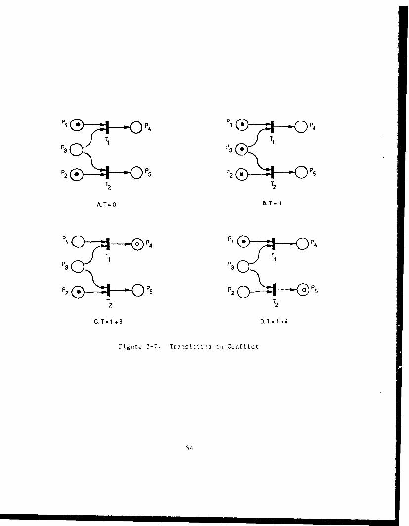
PI P4 P1 P
T, T,
A.T.O B.T- I
P1 0 P4 1 p P4
P3 "3
T2 T2
C. T. 1+a3, 0-I +a
Figuxre 3-7. Trancitttone {In Conflict
54

not well defined. However, the decision rule at P3 specifies the transitionto which the token in P3 is allocated, and so resolves the ambiguity in a welldefined manner.
The final aspect of a transition is the mechanism which determines thevalues of attributes attached to newly created tokens, called an attributemap. Like timing models and decision rules, attribute maps may be determi-nistic or stochastic, or may be dependent on external parameters. The mostuseful form of attribute maps deduces attribute values for newly createdtokens from attribute values carried by tokens destroyed in the same firing.
3.3.4 Arcs/Petri Nets
The connectors between places and transitions are called arcs. Only onebasic constraint restricts the placement of arcs in a STAPN: arcs can onlyconnect places to transitions, or vice versa; they can never connect places toplaces or transitions to transitions. In addition, we impose two additionalconstraints, not absolutely necessary to Petri net theory, but which make formore meaningful measures.
First, every place must have at least one arc leaving it. This precludesthe obvious degenerate situation where toketis pile up in a place ad infinitum.(There may be less obvious cases where this occurs due to some pathology of thePetri net, out these cannot be ruled out by simple topological constraints.)
Second, multiple arcs between one place and one transition are prohibited.Often these are used to create or destroy several tokens in one place simul-taneously. However, the use of multiple arcs significantly complicates thederivation of relations between measures in two or more models. Moreover,activities modeled by multiple arcs can be modeled by equivalent nets withsingle arcs, albeit with a slight increase on the model's complexity.
A collection of places, transitions, and arcs which satisfies these con-straints forms a Petri net. With the addition of timing models, decisionrules, and attribute maps, the Petri net becomes a STAPN. With one otherpiece of information, the STAPN becomes a complete model of a system.
The additional information is the initial marking of the net. A markingcompletely describes the state of the STAPN. It includes the number of tokensin each place, whether each token is available or unavailable, and the attri-bute values attached to each token. It also includes, for every unavailabletoken, the amount of time remaining until the token becomes available (thiscan be considered to be an attribute carried by all tokens).
The marking of a STAPN captures ail of the rnmory of the process whichit models. It is rilatively eatiy to show, by direct construction, that:
Fact I : Given _•tTAIN, and the markinj• of that STAPN at any time t.If t-chu- imiing models, decisiou rules, and attributeaps do notdepend 'm uxtern•] parameters, then the arobahi t' distribution
55

over the set of markings at any future time t+T is conplet,.ly deter-mined. If the timing models, decision rules, andg--trfY-Tite maps aredeterministic, then a unique marking for any future time t+T is com-pletely determined.
As an example of a complete STAPN, consider Fig. 3-8, which shows :1 networkand its initial marking at Lime zero.
Sprwing
Buffer Start Process End
Creation
Free
Figure 3-8. Example STAPN
This system operates as follows. The token in SPACING immediatelyenables CREATION, which places a token both in BUFFER and back in SPACING.If the timing model for this token is deterministically zero, then CREATIONcan fire immediately. More realistically, the timing will be nonzero, sothe token rests in SPACING before enabling CREATION again. Once this hap-pens, this cycle repeats: tokens are intermittently deposited in BUFFER adin. nitum.
There is another set of events that are partially coordinated with theCREATION process. These begin when the first token in BUFFER becomes avail-able. START fires, and when the token created in PROCESS becomes available,END fires and restores a token to FREE. However, if the time to become avail-able in PROCESS is long compared to tile time in SPACING, more tokens will havearrived in BUFFER before the token In FREE becomes avallable. Alternatively,if the time spent in PROCESS arid FREE Is small compared to thle tine spent inSPACING, the FREE token will wait for the next arrival ta BJFFER beforte firingSTART.
56

Overall, then, this is a model of a source of tokens which are stored ina buffer until a resource becomes free. Then, a Rrocess starts; when it ends,the resource is freed up and made available to work with another token in thebuffer. (Irn fact, if the timing models for SPACING and PROCESS are proba-bilistic with exponential distributions, and all other timing models are zero,this is identical to the simplest model from queuing theory: an M/M/l queue.More genprally, any queuing theoretic model can be represented by a STAPN; theconverse is not true.)
3.3.5 Compiexitj_/Jierarchies_
How can STAPNs handle this kind of complexity which IDEFo was designed todeal with? As mentiorei in Section 2, the normal mechanism for managing com-plexity is to organize knowledge ini a hierarchy. Can STAPNs be arranged in ahierarchy? As we will see in subsection 3.5, the answer is "yes" -- one canconsider a large STAPN to be an interconnection of subnetwcrks, each of whichis a STAPN itself. Each of these subnetworks may be furthe: divided intosubSTAPNs, and the process iterated until each subnetwork reduces to a singleplace or transition.
In addition, timing models, decision rules, and attribute maps whichappear in a crude STAPN model of a system may be quite complex. Rather thanleaving them a, primitive entities, their descriptions may expand into entireSTAPNs when more detail Is added.
3.3.6 The "Box Node"
In order to manage the hierarchical complexity typical of C 3 systemsand, more specifically, to be able to represent successively higher levels ofaggregation of other Petri net primitives in simple graphic form, ALPHATECHhas added the concept of a "box node" to standard Petri net representations.
In the formulations we have described so far, STAPN models appear as flatgraphs even though the C 3 systems they are intended to represent are hier-archical in nature. Consequently, the STAPN model of a C3 system reveals allof the details of that sybtem without any organization in this presentation.To capture the hierarchical nature of C3 systems, ALPHATECH created a newPetri net primitive -- the box node. Box nodes, which are represented in aPetri net dia/raw as rectangles with a darkened stripe in the diagraus, areused to cluster and conceal other Petri net primitives -- places, transitions,and other box nodes -- which form a subnetwork or submodel (see illustrdtionin Fig. 3-9). A stibmodel concealed within a box node is incorporated as asingle unit into a model under construction.
The use cf box nodes is analogous to the use oi sibroutines in modularprogramming and affords the same benefits. Box nodes conceal detail and allowthe system analyst to work at a level of abstraction that is hl.gher than thelevel of places and transitions. Box nodes can be arbitrarily complex. Mostimportantly, box nodes allow the development of standardized process models
57
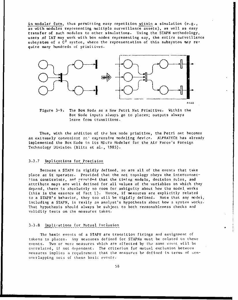
in modular form, thus permitting easy repetition within a simulation (e.g.,
as with modules representing multiple surveillance assets), as well as easytransfer of such modules to other simulations. Using the STAPN methodology,users .of IAT may work with box nodes representing say, the entire surveillance
subsystem of a C 3 system, where the representation of this subsystem may re-quire many hundreds of primitives.
A-3o43
Figure 3-9. The Box Node as a New Petri Net Primitive. Within theBox Node inputs always go to places; outputs alwaysleave from transitions.
Thus, with the addition of the box node primitive, the Petri net becomesan extremely convenient an.' expressive modeling device. ALPHATECH has alreadyimplemented the Box Node in its Micro Modeler for the Air Force's Foreign
Technology DivisiorL (Blitz et al., 1985).
3.3.7 Implications for Precision
Because a STAFN is rigidly defined, so are all of the events that takeplace as it operates. Provided that the net topology obeys the interconnec-lion constraints, anl -rrnvidod that the timing models, decision rules, andattribute maps are well detined for all values of the variables on which theydepend, there is absolutely no room for ambiguity about how the model works(this is the essence of Fact I). Hence, if measures are explicitly relatedto a STAPN's behavior, they too will be rigidly defined. Note that any model,including a STAPN, is really an analyst's hypothesis about how a system works.That hypothesis should always be subject to both reasonableness checks andvalidity tests on the measures taken.
3.3.8 Implications for Mutual Exclusion
The basic events of a STAPN are transition firings arid assignment oftokens to places. Any measures defined for STAPNs must be related to these
events. Two or more measures which are affected by the same evenit will becorrelated, if not dependent. The criterion for mutual exclusion betweenmeasures implies a requirement that the measures be defined in terms of i.cn-overlapping sets of these basic evenits.
58

Thus the formal structure of STAPNs provides a step towards the goal ofindependent, and largely uncorrelated, definitions of C system measures ofperformance. The requirement for mutual exclusion atnong the sets of eventswhich underlie measure definitions are satisfied in Appendix A, where canon-ical measures are developed.
3 4 RELATIONSHIPS BETWEEN THE PHYSICAL AND MATHEMATICAL CONSTRUCTS
Earlier we alluded to certain analogies between the real C systems andthe abstract mathematical constructs inherent in STAPNs. This section dis-cusses each of these analogies and sets out the axioms of our approach.
The reader will recall the viewpoint presented in subsection 3.2:
A Command and Control system, and its environment, consist of anumber of objects moving through neighboring geographical regionsor flowing through various interconnected facilities, all in apartially coordinated, asynchronous fashion.
Now consider a simple description of STAPNs:
A STAPN describes how a number of tokens move among interconnectedplaces in a partially coordinated, asynchronous fashion determinedby transitions.
The analogies between each of the terms in these statements is made moreprecise below.
3.4.1 Tokens: Objects
First, messages move through a C system and objects move through itsenvironment. Tokens move throagh STAPNs. In general:
A.serti-jn I: All objects tha- move through a Command and Controlsystem or its environmen+ -- be represented by tokens movingthrough a STAPN.
As used in subsection 3.2, "object" is a general notion. Objects include con-crete entities such as submarines, people, and messages. Objects also includeconcrete manifestations of more abstract notions: the position of an indi-cator that represents the DEFCON state, the location of warfighting materielthat represents a state of combat readiness, or the armament on a close airsupport aircraft that represents its capabilitits.
Unlike many objects, which exist permanently, tokens are cre;ated anddestroyed regularly. For tukens to represent real objects, a succession oftokens most be used to re,)resenL an individual object, by dividing the life-tine of that object into separate segiaents of timre. Different tokens willrepresent the continuous existence object during each segmenL. For example,
59

a single aircraft may fly through several geographical regions; a differenttoken will represent that aircraft in each region. The sequence of tokensthat represents the aircraft corresponds to the sequence of regions throughwhich the aircraft travels.
As the above example shows, the correspondence between token and objectscannot be one-to-one. However, we can infer:
Conclusion 1: At any single instant of time, there should exist aone-to-one correspondence between tokens and (generalized) 2•yscal1objects.
3.4.2 Places: Regions, Facilities
Objects move from region to region; messages move from facility tofacility. In discrete models, movement is instantaneous and objects spendalmost all of their time in regions and facilities. Tokens rmove from place toplace, and spend almost all of their time waiting in places. Thus we claim:
Assertion 2: All facilities in a Command and Control system, orregions in its environment, can be represented by places in a STAPN.
Generally, this assertion implies that places represent processing: thatthe time a token stays in a place is related to the activities which Involvethe corresponding object in the real system. It takes time to cross a geo-graphical region; it takes time to handle a message. Neither aircraft normessages can proceed until certain amounts of time have elapsed. Tokens muststay in places until they become available; timing models capture the durationof this wait. Thus we have:
Conclusion 2a: Transit and processing times must be representedby tining models in a STAPN.
In reality, objects may leave one region for any one of several neigh-boring regions; messages may be forwarded to one of a number of faciliticsconnected to a sender. The selection of an alternative region or facilitydepends on random effects, standard operating proceedures, and operationalpolicies. Each place in a STAPN has an associated decision rule which deter-mines which of several arcs a token will follow out of a place. We concludethat :
Conclusion 2b: Policies, procedures, and random events whichinfluence the paths which objects follow must be modeled bydecision rules in STAPNs.
Thus if a place represents an ASW sector for a Naval battle group, then atiming model will describe the time required by hostile submarines to movethrough the sector, and a decision rule will model the process which deter-wines the sector Into which the submarines move next.
60

A limitation of this approach becomes apparent when regions or facilitiescan change over time. If a sensor or weapon moves, then the regions which
form their fields of view or fire change. !f a battle group approaches a
coastline, it redefines its ASW sectors to exclude areas where submarinescannot operate. In space, orbital motions cause communications links to be
established and broken regularly. If a C3 system reconfigures itself after
sustaining damage, then its facilities and their interconnections change.While one can envision a STAPN model which tracks these changes, the notionsrequired to formalize this process have not yet been developed.
3.4.3 Transitions: Boundaries, Events
Transitions demarcate and coordinate the flow of tokens. Consider thephysical analogs of each of these roles separately.
Along with the correspondence between objects and tokens, there must be a
correspondence between events in the real system, and the events which createand destroy tokens. Tokens endutz in a place while the corresponding objectoccupies a certain region or faciliLy; tokens leave a place when the objectleaves. Tokens leave when a transitio•i fires, so we must have:
Conclusion 2c: There is a one-to-one correspndence between bound-ary crossings (between Aegions and/or facilities) by obects Inareal system, and transition firings in a STAPN.
Continuing the ASW example, a submarine crosses a boundary when it enters orleaves a sector; acoustic energy crosses a boundary when it passes from theocean to the piezoelectric crystal in a hydrophone; a message crosses a bound-ary when a sonar operator tells the ASW officer on duty about a new detection.In a STAPN model of this process, transition firings represent each of theseevents. RecAll that transition firings are instantaneous; so are boundarycrossings if the boundary is infinitely thin and the object crossing it alwaysmoves with nonzero speed.
Turning to the coordination role, transitions force some tokens to waituntil others become available. The physical analogy to this occurs whenobjects or messages are prohibited from crossing a boundary until otherobjects or raessages are in suitable locations. In general, we suggest that:
Assertion 3: Coordination occurs in a real system only when oneobject or message ray be forced to wait until some other objector message is ready to move on.
This is less an axiomatic statement than a particular definition of coordina-tion. Nonetheless, it captures the essence of real coordination schemes inasynchronous systems. In fact, it even applies to synchroaous systems, ascertain activities can;iot begin until a global clock "tick" reaches them.
?otr net transitions shotild be famillar tr) users of PERT charts: atrasiTion provides exactly the same coordination mechanism as do PRT mcoels.
61

In fact, standard PERT charts are identical to STAPNs which have (a) deter-ministic timing models, (b) no decision rules, (c) no attributes, and (d) no
loops formed by any series of arcs. Various extensions to standard PERTmodels include some forms of these other features, excluding loops. Just asPERT models have been widely used in scheduling applications because of theirflexibility and simplicity, so their extensions, namely STAPNs, convey thesame benefits.
3.4.4 Complexity/Hierarchies
In Section 2 and subsection 3.2.6, we saw that hierarchical rc:presenta-tions of C3 systems were necessary to prevent their inherent complexity fromoverwhelming a viewer. In subsection 3.3, we saw that there is a potentialfor complex STAPNs to be either divided into subSTAPNs or expanded at theirtiming models, decision rules, or attribute maps.
If analogies, consistent with assertions 1-3, can be established betweena gross model of a C3 system and reality, as well as between a refined modeland that same reality, then there ioust be relationships between the gross andrefined models. Some general forms of these relationships are presented inAppendix A.
3.4.5 Implications for Measurability
What does iU take to establish strict analogies between events In a realC 3 system, and events in a STAPN model of that system? What do we look forIn the real systems to be studied, and how do we translate what we find intoa STAPN model? How does all this help ensure that variables defined in terlasof the STAPN are in fact measurable in the real system?
A summary of the process discusbed above suggests that STAPN representa-tions can be built systematically if we:
I. specify the objects that move through the system, and definethe token attributes that are needed to characterize each,
2. specify the regions or facilities in which objects may bestored, and define a place for each,
3. specify the boundaries which objects cross as they move betweenregions and facilities, and define a transition for each,
4. where objects must reside in regions or facilities for a periodof time before moving on, define a timing riodel for the corre-sponding transition/place pair,
5. where objects may depart a region or facility along one ofmultiple paths, define a decision rule for the correspondingplace,
62

6. where attributes may change as an object crosses a boundary,define an attribute map for the corresponding transition,
7. where coordination can happen, define the transitions (andrelated tokens and places) which model the coordinationmechanism.
If we follow these steps, the correspondence between reality and a STAPNis based on the definitions of objects, the regions or facilities in whichobjects may reside, and the boundaries between regions and facilities. Sup-pose that this correspondence is made precise for each token, place, andtransition in the STAPN, and that we impose the following guideline whendefining behavioral variables:
Assertion 4: All measures will be defined in terms of the STAPNelements, so that the measures relate to transition firings and thecreation, storage, and destruction of to'.ens in places. For thesemeasurestobecomplet.eelydefined, there will be an explicit way to
evaluate their values by observing the behavior of the STAPN model.
Let the evaluation mechanism be captured in some algorithm, which acceptsa list of firings, creations, storage, and destructions and which produces thevalue of a measure. Then it is reasonable that:
Conclusion 4a: Values of measures defined on a STAPN can beobtained for the corresponding real system, using the algorithm forevaluating those measures for the STAPN, by replacing (a) transitionfirings with boundary crossings by objects, (b) token creations byobject entries into regions or facilities, (c) token storage byobject residency in regions or facilities, and (d) token destructionby object departures from regions or facilities.
Moreover, since each object, region, facility, and boundary is defined interims of physical entities, which are observable, we conclude that:
Conclusion 4b: STAPN variables consistent with Assertion 4 aremeasurable in the real system.
Btcause representations of C3 systems are not unique, difierent analystswill undoubtedly choo0e to define objects, regions, and boundaries in slightlydifferent ways. However, as long as they are all physically meaningful, andas long as the correspondences between real and STAPN elements are carefullydefined, we can feel comfortable about defining measures for the STAPN andeYpect. them to carry over into valid measures for the real system and a stan-dard method for evaliat ing them.
The reader i.- referred to Appendix A for further detail.
63

3.5 RELATIONSHIP OF STAPNs TO EXISTING METHODS OF SYSTEM REPRESENTATION,MODELING, AND ANALYSIS
In Fig. 3-10 we show the relationships among all of the various IATelements previously defined. Along the bottom of the figure are the varioustechniques used by systems analysts to gather and structure data about C 3
systems. As indicated, these can be employed, as individual familiaritywith each one dictates, to obtain as much of the process and connectivitydata required to develop a detailed-level C3 system process model using theStochastic, Timed, Attributed Petri Net (STAPN) modeling method describedearlier in this Section. From the maodel structure itself, it is then possibleto define a complete, nested set of Probability, Rate, Occupancy, and Delay("PROD") measures for the C3 system.
However, in order to obtain quantitative values for these measures, weneed to know two things: (1) the performance capabilities of the variousresources, and (2) the specific resource-to-process assignments. Of partic-ular importance here is the data on shared resources, i.e., where one resourceis time-shared among several processes. Then, to complete the picture we needscenario data to define the specifics of both enemy target and friendly weaponsystem actions.
Evaluation of a single target moving through the system under variouscircumstances can produce a PERT or critical path assessment. On the otherhand, a full multi-target scenario will require more sophisticated evaluationtechniques such as the application of queuing network theory or, for morecomplex models, the use of simulation; in either case, the full range of sta-tistics on probabilities, rates, occupancies and delays ("PROD") will becomputed. As the model becomes defined in increasing detail, additional dataneeds will become apparent to the analyst. Discussions of example queuingtheory and PERT/CPM analyses can be found in Sections 5 and 6, respectively.
As indicated by the horizontal dashed line in Fig. 3-10, the foregoingrepresents the set of current IAT elements and how they relate to one another.It involves two of the four decomposition dimensions (process and resource)and four of the six types of measures (system capability, mission environment,system performance, and system effectiveness) described in Section 2.
The survivability of various C 3 functions can be evaluated in a simpli-fied manner using the static, set-theoretic method of Wohl et al. (1981).This involves (1) defining a specific function in detail and determining thequantity and type of resources required to support that function; (2) identi-fying the resources actually available or assignable to carry out the func-tion; and (3) determining the probability that the requisite number and typeof resources remain available after a given (specified) attack on the C3 sys-tem. Thus, functional survivability can be assessed in a gross, static,"before-and after" sense. However, we are not yet at the point where C 3 sys-tem survivability can truly be evaluated in detail. The main problem here isthat little work has been done to define carefully the various factors affect-ing functional survivability other than the aforementioned gross measures.For example, time averages may not make sense because of intervening changes
64

,VAL VAT IO SuftMABIrTY
( OikMGL3 70 C3
C's~~PACC S..OE2osC
s tN
PEFI sa~MJC S
FrD ATA E o,-
5 AVA... ,tOYPS~~iL
fvxuZE CjTIASSC AM4!4SCPBLT
DE
PAIIS 1ATOAG/UJAS !..A T!!
S,;lV 3-AI. OAT d AosspA~~TFEcie~

in C3 system topology or structure; while ensemble averages may be question-able because the system structure may change at different times in successivereplications. Such evaluation would have to involve analysis of the dynamic
reassignment of resource capabilities in the system, and these are determinedby the organizational constraints (i.e., lines of authority, responsibilityand coordination) as well as by changes !n the C3 system structure due to
enemy action, etc. (See the end of subsection 2.5 for a discussion of prob-lems associated wiLh attempting to improve a C 3 system arch!tectore.)
3.6 USING ýTAPNs TO MODEL HUMAN ACTIVITIF:S
In this section we examine how STAPNs can be used to represenL a widerange of human activities in C3 systems. These activities range from psycho-motor tasks such as those involving both simple and complex (disjunctive)
reaction tines to higher-level cognitive tasks such as the Hypothesis andOption election tasks in the SHOR paradigm (Woh] , 1961).
The following five illustrative cases demonstrate the applicability ofSTAPNs to human behavior modeling and specifically to representing the SHORParadigm. From them, it is clear that more complex concatenations of humaniactivities can indeed be represeited using STAPNs.
66

3.6.1 Case I: Simple Reaction Time Tasks
Sample Task 1: If light comes on, push buttom immediately.
Sample Task 2! If message is received, send acknowledgementimmediately.
Measure: Reaction time (tr).
State 1: - 1 Light off (token not present)
State 2: Q . Light comes on (token presentbut unavailable)
State 3: (O ( Light is on, perception and& /A -.<D cognition occur (token becomesavailable after tr seconds)
State 4: Button is pushed (transition fires)
Note: tr f(light brightness, message length, etc.)
Figure 3-Ai. Petri Net Representation, Case I
S ) . R If S then R
SIMPLEDISCRIMINATION
(ON/OFF)
Figure 3-12. SIIuR Representatton, Case I
67

3.6.2 Case 11; Complex (Disjunctive) Reaction
Sample Task 1: There are three colored lights that can come on:Red, Yellow, Green. If Red comes on, push button#'l; if yellow, #12; if Green, #3.
Sample Task 2: These are three possible formatted nrtGsagei; thatcan be received: R, Y, or G. If R, respond withacLton 01; if Y, #12; if G, #/3.
State 1: 11 . 1 I No lights on (no tokens present)
State 2: -- ¶ Red light comes on (Red tokenpresent 'hut unavailAble)
AEO'TOKEN 1 3
State 3: 1- 1 Red light remains on; perception,
discrimination, and cognition occur
2 (Red token becomes availiable aft'--t
RED,• tr seconds)1OKEN ___,_ 3
State 4: - 'BO utton 01. is puqlhed (Red trans IA oa* '+_* f iri-u, Red token disappears, rre"w
- . Q 2 token is created in place ;'.I)
r-3 3t p tiA
Figure 3-13. P~eLri N,(:-L R cp e eir •; IL aLtOiI, C a;|•; TI
68

Decision Rule: If Red token is present and available, red transitionfires, etc.
Note: tr f(number of lights or colors, difficulty ofdiscrimination, etc.)
S R If S 1 then R 1 , etc.
S2 R2
$- R3 3
COMPLEXDISCRIMINATION(LIGHT COLOR)
Figure 3-14. SHOR Representation, Case II
69

3.6.3 Case III: Hypothesis Selection Task
Sample Task: Tokens A, B, and C have attribute sets Ai, Bj, and C%-
Token attributes represent "indicators" (e.g., diagnosticsymptoms and their confidence levels).
Task: Select that hypothesis that has the greatest number ofhigh-confidence indicators.
Measures: Processing time, confidence level in chosen hypothesis.
TOKENS41A B 41C
ýH
ALLTOKENSGOTO H.sVALL 0 - -<
(r1 PLACES
j kR-3606
111 Decision Rule: If Al, B3, and C 6 , then HI
H2 Decision Rule: If Al, B1 , and C2 , then H2
etc.
Figure 3-15. Petri Net Representation, Case IlI
S n H
DISCRIMINATION& ORGANIZATIONOF ATTRIBUTES
Figure 3-16. SHIOR Representation, Case III
70
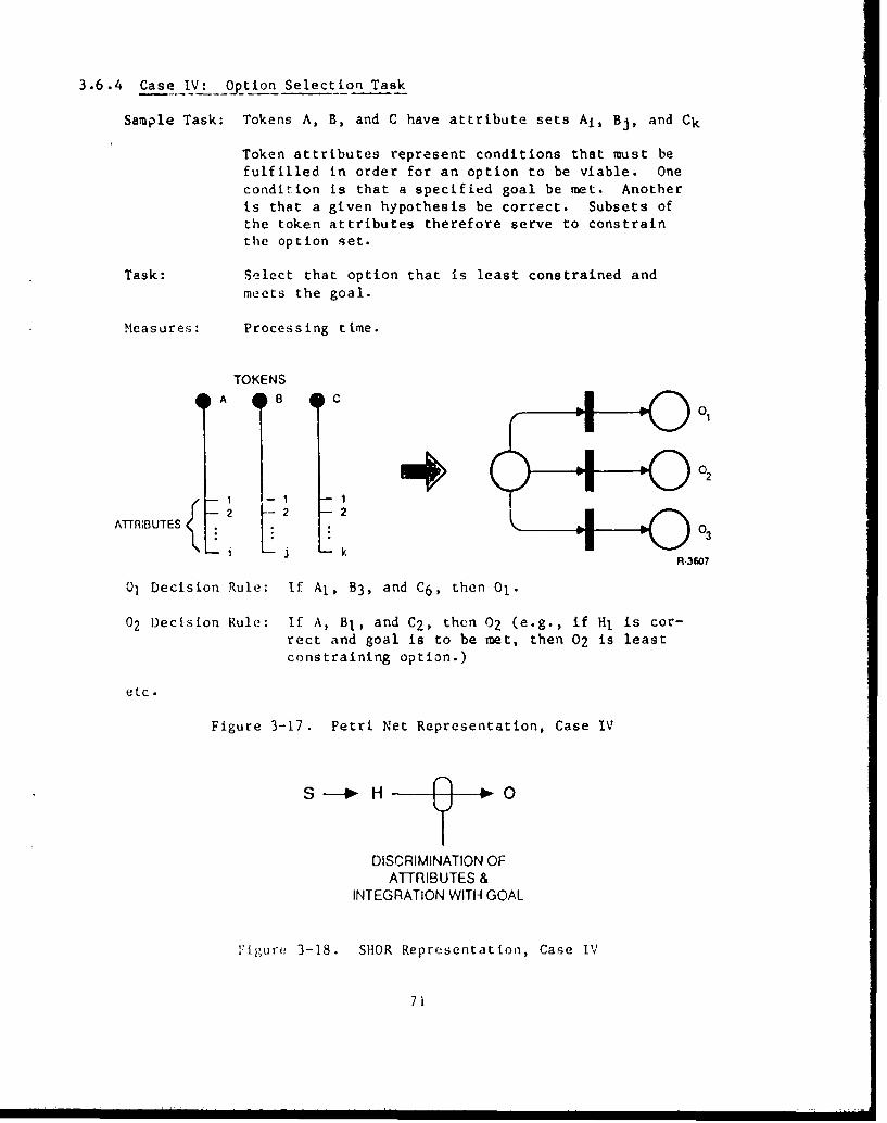
3.6.4 Case IV: Option Selection Task
Sample Task: Tokens A, B, and C have attribute sets Ai, Bj, and Ck
Token attributes represent conditions that must befulfilled in order for an option to be viable. Onecondition is that a specified goal be met. Anotheris that a given hypothesis be correct. Subsets ofthe token attributes therefore serve to constrainthe option set.
Task: Select that option that is least constrained andmeets the goal.
Measures: Processing time.
TOKENS
A 4 B 4 c C1 _* "
4, 02
1 -
ATTRIBUTES{ 03
R.3607
01 Decision Rule: If Al, B3 , and C6 , then 01.
02 Decision Rule: If A, BI, and C2 , then 02 (e.g., if Hl is cor-rect and goal is to be met, then 02 is leastconstraining option.)
etc.
Figure 3-17. Petri Net Representation, Case IV
S • H -- { O
DISCRIMINATION OFATTRIBUTES &
INTEGRATION WITH GOAL
Figure± 3-18. SHOR Representation, Case IV
71

3.6.5 Case \ : Higher Level Cognitive Task: Hypothesis Generation and Testing
Sample Task: Find a rational "explanation" (hypothesis) for thepresence or existence of Ai, Bj, and Ck.
Method: (1) Look for analogies to previous situations
or to other cases.
(2) Find that analogy (141) that best explains oraccounts for the presence of Ai, Bj, and Ck.
(3) Identify additional token attributes that
would have to be present if H1I were tr.ie
(e.g., Cn).
(4) Test to see whether they are present.
If so, accept lii.
If not, try F. (next best analogy).
(5) etc.
Same as Case 111, except for token C:
C
2
k
2 ADDITIONALATTRIBUTES IF
: • H1 IS TRUE
R- 3608A
Figure 3-19. Petri Net Representation, Cas;e V
72

Appendix B contains several additional examples of how various types ofhuman interaction can be represented using STAPNs.
3.6.6 Relationship to Rasmussen's Task Taxonomy
The foregoing sample cases are also instructive from another vie,'-oint.Several years ago, Rasmussen proposed a simple taxonomy of human tasks whichhas been extrewely useful in organizing thinking about human behavior insystems (Rasmussen and Rouse, 1981). In essence, he said that such behaviorfalls into one of three classes:
- Skill-based
- Rule-based
- Knowledge-based
Skill-based behavior is exemplified by human operators performing lower-level,more "mechanical" psychomotor tasks such as the reaction time tasks in CasesI and II above, as well as more complex tasks such as those involving trackingbehavior. Rule-based behavior is exemplified by human operators and/or deci-sionmakers perforoing intermediate-level cognitive tasks such as simple pattern-matching, and hypothesis and option selection tasks in whic¢ the alternativesare known, as in Cases III and IV above. Knowledge-based behavior is exempli-fied by human dectsionmakers performing higher-level cognitive tasks such ashypothesis and option generation tasks in which the alternatives are unknownand must be developed as part of the task, as in Case V above. This case isespecially interesting since it assumes that decisioninakers are strongly de-pendent upon historically analogous situations as a basis for generating newhypothesis and/or option alternatives. Evidence for this assumption is con-
tained in the work on mental models by Larkin et al (1980); on analogical rea-soning by Klein and Weitzenfeld (1978); and on historical reasoning and itsimpact by Neustadt and May (1986).
3.7 GUIDELINES FOR CONSTfRUCTING IAT PROCESS MODELS WITH STAPNs
,uilding IAT mod, :s of physical processes should proceed in three stages:
$tave I:lnitializa~tion
* Scope the problem.
S Ide-it ily boundaries and data or objects crossing thebou dda ries.
* S;: uil a list of data collection goals and criteria,
73

Stage 2: Build a Baseline Model
"* Construct a "mid-level" model of the complete system.
"* Carry out data collection and assess whether Stage 1goals and criteria have been met.
Stage 3: Refine the Stage 2 Model
"* Elaborate tie model structure as needed to insureconsistency, completeness, and parsimony.*
Activities to be pursued at each stage are listed below.
3.7.1 Stage 1: Initialization
1. Define the boundary of the system to be modeled. Think of thisin physical terms (e.g., the NCMC complex). Express Khe boun-dary in terms of data/material flows (e.g., the arrivng mes-sage traffic, the departing message traffic, etc.).
2. Decompose the input/output flows into their finest elements(i.e., if two types of message might be processed differently,they form two token flows, even if they arrive through the samephysical channel). Each elementary token flow defines a tokentype, to be placed on the list of token types, along with anannotation.
3. Define a transition for each token type to cross the boundaryof the system. These transitions would be labeled "Detectionmessage from sensor 3 arrives at NCMC" or "Operational ordersent to SAC from NCMC," etc.
3.7.2 Stage Z: Build a Baseline Model
Maintain separate lists of all defined items including:
* token types
* places
* transitions
* branches
*Sec discussion in subsection 3.4 above.
74

as initialized above. Each item on a list represents a data collection goal:fill in all the information described in Section 3.4.5. Items with all slotsfilled in can be placed on a second list. By definition, a model is completewhen all items are removed from these lists. Moreover, it is easy to guar-antee consistency as each item is filled in.
Note that one may have t' add items to these lists as slots are filledin. For example, if a token type "Detection message from sensor 3" is defined,that item cannot be taken off the list until two transitions, marking both thegeneration and disposal of these messages, are added to the transition list.
The order in which items are taken from these lists to be completed canbe arbitrary. It should be selected to suit the data collecto:'s constraints.A natural order is to walk through one processing path at a time. For example:
Q: Where do detection messages from sensor 3 go?
A: (Definition of a new place: facility, resource.)
Q: How long does it take to get there?
A: (Timing information.)
Q: What happens next?
A: (New branch or transition.)
Q: Must something else happen first?
A: (New token-type.)
etc.
3.7.3 Stage 3: Refine the Stage 2 Model
While the baseline model way be guaranteed to be complete and consistent,it may not be parsimonious. The lack of parsimony can be found in timingmcdells and decision rules wh: depend on non-local state information. Addi-tional network structure to reduce these models should be added.
3.8 PROCEDURES AND GUIDELINES FOR SYSTEMATIC GENERATION OF SETS OF NMEASURESFROM STAPNs
3.8.1 Step I: Construct the Top Level Model
Section 2 presc:ted arguinent.s in favor of a sysLoruatic method to identifya set of variables which describe the behavior of a Command, Control, andCoMrInunictC ions systen. I1.n this section and Appendix A the founidations for
75

such a method have been laid by introducing Stochastic, Timed, AttributedPetri net (STAPN) models, their canonical measures, and ways to organize suchmodels in a hierarchy. This subsection weaves these various threads into asingle, self-contained tapestry: an iterative process that simultaneouslymodels C3 systems and extracts a hierarchy of variables that measure theirbehavior.
The resulting method has five major steps, repeated until the models andmeasures reach a level of detail sufficent for the purpose at hand. Eachsubsection of this section delves into the details of each step, first in theabstract, and then in the specific context of a generic tactical air defensemission. The air defense example provides concrete illustrations of eachaspect of the method. A few heuristic guidelines, generated in the course ofexercising the methodology on the air defense example, bridge the abstract andconcrete. These guidelines result not from theoretical analyses, but frompragmatic concerns which seem, at least in the limited context of air defense,to contribute to more acceptable and useful sets of measures.
A secondary product of the air defense example is empirical evidence thatcommon behavior measures may apply to C3 systems (including humans) that sup-port a common mission area. This statement certainly applies to highly aggre-gate models; it may break down as the hierarchy of models becomes successivelymore specific. Nonetheless, a common set of high-level behavior measuresdoes seem to exist for air defense and appears to exist as well for the otherlimited examples (SIMCOPE and NORAD MWC) described in Volume II.
Procedure
The first step of the methodology builds a highly aggregated STAPN modelof the system under study. The purpose of this step is (a) to capture theessential objectives of the system in a STAPN framework, and (b) to establisha starting point for later iterations which refine and extend the STAPN model.The top level model need not be complicated, as the successive iterationsthrough the methodology provide ample opportunity to add detail.
The basic process for building a STAL'N model for a system was establishedin subsection 2.5. Repeated here, the seven substeps required to buiid a c•m-plete SYAPN model are:
I. Specify the objects that move through the system, and define thetoken attributes that are needed to characterize each,
2. Specify the regions or facilltie• in which objects may be stored,and define a place for each type of token which can be stored ineach region or facility,
3. Specify th,_- boundaries which objects cross as thuy move betweenregions and facilities, and define a transition for each,
76

4. Where objects must reside in regions or facilities for a periodof time before moving on, define a timing model for the corre-sponding transition/place,
5. Where objects may depart a region or facility along one of mul-tiple paths, define a decision rule for the corresponding place,
6. Where attributes may change as an object crosses a boundary,define an attribute map for the corresponding transition,
7. Where coordination can happen, define the transitions (and relatedtokens and places) which model the coordination mechanism.
Fortunately, if the only objective is to identify behavioral measures,the final four substeps are optional. Certainly they are necessary to definea complete STAPN model. However, in subsection 2.5 it was shown that thecanonical measures for a STAPN model are defined by places, transitions, andinterconnections alone; the timing models, decision rules, and attribute mapscontribute to evaluation of the variables, but are unnecessary for the iden-tification of variables. Since the purpose of this work is the latter (seesubsection 1.6), only the first three substeps are relevant to the generalmethod.
Guidelines
Two general advisories apply to the construction of the top level model.First, if a model. directly relates to generally accepted statements about thepurpose and structure of the -.ystem which it represents, then it (and itsrefinements) will be more readily accepted. Since the model which representsa system Is not unique (see subsection 1.5), we can always anticipate differ-ences of opinion about the correpondence between model elements and reality,or about the appropriateness of the level of detail preserved or suppressed inthe top level model. Little can be gained by offering additional opportuni-ties for disputes about the scope or purpose of a system. Such issues haveoften been discussed at great length in other forums. References to publisheddoctrine, official. definitions, and generally accepted viewpoints provide afirm and easily justified starting point for the methodology.
Secondly, humans (and particularly engineers) have a great deal of diffi-culty describing a system at a crude level of detail. Their strong tendencyis to critique a simple model of a system by pointing out numerous featureswhich are not represented in that model. In the context of our methodology,this tendency is counterproductive: the purpose of the top level model is tocapture only the broadest aspect of the system -- not every detail. More thana modicum of discipline is needed to keep the top level model simple, and to
relegate the details to later iterations of the method.
In summary, two guidelines for Step I of the rmethodology are:
77

1. M~intaiiu cledf cuutectIonj between the top level STAPN modeland previously established views on the scope and purposee of
the system.
2. Keep the top level model as simple as possible, leaving details
for later refinements.
3.8.2 Step II: Generate all Canonical Measures
The STAPN model serves as an intermediary between reality and the mea-
sures sought. From the model, we can extract the set of canonical measures --
a set which is unique and well defined once the model is established.
Procedure
The second step of the methodology uses an existing STAPN model of the
system under study as the basis for deiinitions of a large set of measures.The purpose of this step is to generate a set of measures which are (a) mutu-
ally exclusive (describe nonoverlapping sets of events) and (1j collectively
exhaustive (complete with respect to the STAPN model).
The principal challenge of this step is to establish notation that iseasy to extend through several levels of a hierarchy. To this end, conven-tions are adopted similar to those used by several other structured decompo-
sition methods:
I. Formally name each model at level N+l by appending a uniqueletter, in alphabetical order, to the name of the model atlevel N of which it is a refined submodel.
2. Formally name each place in a model with a letter P, using asubscript constructed as described in (4) below.
3. Formally name each transition in a model with a letter T, usinga subscript constructed as described in (4) below.
4. Construct subscripts by appending a numerical index, in ascendingorder starting with i, to the model name.
Canonical measures are straightforward to generate from a STAPN model ofa system. The four substeps required to identify the canonical measures are:
I. To each output arc of a place Pi, leading to some transition Tj,assign a probability measure Pij.
2. To each transition Ti, assign a rate measure Xi.
78

3. To each place Pi, assign an occupancy measure ni.
4. To each place Pi, and to each output transition Tj for Pi,assign a delay measure Ti,
Note that the formal notation for each measure follows directly fromthe notation for places and transitions. Naturally, informal names can beattached to places, transitions, and measures for convenience. However,unless the model is to be extended to only one or two levels of detail, theformal naming method is preferable as it guarantees that each measure has aunique name.
Guidelines
Only one guideline applies to the derivation of canonical measures.Recall that tokens may have attributes. Subpopulations of tokens are implic-itly defined by attributes, as we may divide tokens into groups, with tokensin each group sharing like attribute values. Often, measures may need to bedefined for each attribute subpopulation separately. For example, one maywish to explicitly consider cases where the delay encountered by messagesabout different target types are different, since different message types maybe handled with different priorities, although they follow the same processingpaths. In this case, the delay for each message type, rather than an averageover all messages, is of interest.
Instead of building separate models which depict the processing of eachindividual subpopulation, one can define vector-valued measures. The compo-nents of the vectors are measures for each specific attribute value whichdetermines a subpopulation of interest. Thus if there are four message types,the canonical measures for the model elements which describe the message hand-ling are four-dimensional vectors.
Fortunately, the horizontal relations defined in subsection A.3 apply,componentwise, to vectors of canonical measures as well as to scalar measures.Additional vertical relations may be required to relate components of vectormeasures at level N+I, where subpopulations determined by attribute values maybe broken e-it. t• e--rr- -t level N, where attribute values may not be con-sideritr! at .. i .. _ se relations are generally simple sums and expectations,mimicking the f,,rns discussed in subsection A.5.
Thus the only guideline for Step II of the methodology is:
1. Use vector valued measures when the only distinction betweentokens and the way_ they move through a STAPN is the value ofattributes that they carry.
79

3.8.3 jtea III: Select Primarry.1Mensures
While all canonical measures are physically meaningful and potentiallyinteresting, they are not all independent. The redundant measures may beeliminated without fear of compromising the coverage of the overall set ofmeasures, while simplifying the description of a system's behavior.
Procedure
The third step of the methodology reduces the set of candidate measurescompiled in Step II using the standard horizontal relations developed in sub-section A.3. The purpose of this step is simply to develop a (nonunique) setof independent primary measures.
The basic procedure passes through two phases. The first phase (substeps1 - 4) generates a list of horizontal relations. The second phase movesthrough that list, successively eliminating both relations and measures:
1. Derive a conservation of probability relation between the prob-ability measures attached to the output arcs of each place.
2. Derive a conservation of rate relation between the rate measuresattached to the output transitions of each place.
3. Derive a probability-rate relation between the rate measure foreach transition and the probability measure attached to everyarc leading to that transition.
4. Derive an occupancy-rate-delay relation between rates at theoutput transitions at each place, the occupancy measure at thesame place, and the delay measures between that place and itsoutput transitions.
5. Select any relation remaining on the list.
6. Select any measure appearing in that relation.
7. Solve for the value of the selected measure in terms of theother measures appearing in the selected relation. If this isnot possible, discard the relation and go back to substep 5.
8. Replace all appearances of the selected measure in all remaininghorizontal relations, using the formula from step 7.
9. Discard the selected measure and relation. If any relationsremain, go to substep 5.
Substeps 5 and 6, of course, are the arbitrary decision points whichallow the final set of primary measures to be nonunique.
80

Guidelines
Several guidelines can help reduce the arbitrariness of the selectiondecisions. These guidelines fall into two classes: general suggestions aboutthe measures that tend to be most acceptable to users, and specific revisionsto steps 5 and 6 implied by a literal interpretation of the general guidelines.
Four general ideas about measure selection follow from considerationsof the uses to which the measures will be put. First, in the evaluation ofalternative systems, numerous measures quantify a system's behavior. Nosingle measure captures a concept of good behavior; the multitude of behav-ioral, structural, and socioeconomic measures must be combined into a singlemeasure of a system's worth before final selections can be made. This combi-nation logic can simplified, and made more intuitive, if the sensitivities ofthe overall measure of worth, with respect to individual measures, are all ofthe same sign. Arbitrarily, one can ask that a selected measure has the prop-erty that an increase in its value leads to an increase in the overall worthof the system. Thus a choice between the probability of detection, and theprobability of nondetection, of hostile aircraft should be resolved in favorof the probability of detection, as increases in that measure are usually con-sidered to be good.
Secondly, the basic objective of a C3 system is to deliver weapons tohostile targets before those targets cause any damage. The basic objectiveof the targets is to cause damage before the C3 system can respond. Thisrace between enemy assets and the C3 processes is the essence of C3 systemevaluation, and is most naturally captured by the canonical delay measures:does the time required for an enemy to achieve its objectives exceed the timerequired to arrange friendly forces to meet the threat? Since the occupancy-rate-delay relations allow us to exchange occupancies and delays, they shouldbe used to eliminate occupancies in favor of delays.
Thirdly, the probability-rate relations allow us to exclude either proba-bilities or rates. Except in cases where a natural benchmark (such as physi-cal throughput capacity constraints) exist, rates can be hard to interpret.Probabilities always have such a benchmark: they are always bounded between 0and I. Thus probabilities should be preferred to rates, as the normalizationfor probability measures automatically provides a sense of scale.
Finally, division by zero is not well defined. Step 7 may result inequations involving division, and we should cvoid the possibility that thedenominator becomes zero whenever possible.
Thus the three general guidelines for :asure selection are:
1. Eliminate measures for which decreasing values are usuallyinterpreted as indicative of better systems.
2. Eliminate occupancies in favor of delays when considering anoccupancy-rate-delay relation in substep 5.
81

3. Eliminate rates in favor of probabilities when consider nLaproba ility-rfat te r-ae t on ____ _7
2ue 5
4. Do not eliminate measures which allow equaions in substec_7to have denominators which may become zero.
Mechanically applying these guidelines yields a specific strategy togenerate the set of primary measures, once the horizontal relations have beenidentified. Noting that guideline 4 is not explicitly included, the special-ized strategy for steps 5 and 6 becomes:
5a. If any Conservation of Probability relation remains, select it;otherwise, go to substep 5c.
6a. Select, for elimination, one probability measure in the relationof substep 5a for which a decrease in value is generally consid-ered to be good. (At least one such probability measure exists,since an increase in the most favorable probability must be off-set by a decrease in at least one other.) Continue to step 5cafter the probability is eliminated.
5b. Select the Probability-Rate relation which contained the proba-bility measure chosen in step 6a.
6b. Select, for elimination, the rate measure in the relation ofsubstep 5b. (This rate measure is monotonically relatedto the probability measure in substep 6a, for which a decreasein the rate must also be considered to be good.) Go back tostep 5a after the rate is eliminated.
5c. If any Probability-Rate relation remains, select it; otherwise,go to substep 5d.
6c. Select, for elimination, rate measure in the relation of sub-step 5c. Go back to step 5c after the rate is eliminated.
5d. If any Conservation of Rate relation remains, select it; other-wise, go to substep 5e.
6d. Select, for elimination, a downstream rate measure in therelation of substep 5d. Go back to step 5d after the rate iseliminated.
5e. If any Occupancy-Rate-Delay relation rem.-ies, select it; other-wise, the process ls complete.
6e. Select, for elimination, the occupancy measure In the relationof substep 5e. Go back to step 5e after the occupancy iseliminated.
82

These substeps apply when steady state or time average measures are used;a slightly different selection order should be used for ensemble averages.
3.8.4 SLep IV: Refine Primazy Measures
A STAPN model of a system was built in Step I. Steps II and III devel-oped sets of primary and secondary measures from that model. The measures areprecisely defined in terms of that model. However, the measures will be usedfor the real system, and they may nut yet be precisely defined in terms ofreal events.
Procedure
The fourth step of the methodology uses the list of primary measures tofocus attention on some correpondences between physical elements of a realsystem and abstract elements of the STAPN model of that system. The elementsdeserving further scrutiny are simply those that appear in the definitions ofthe primary measures. In addition, some aspects of the measures themselvesmust be specified. Thus the purpose of this step is to (a) transfer the defi-nitions of primary measures from the STAPN elements to the real system, and(b) to add further pragmatic information to the definitions. The product ofthis step is a glossary which augments the definitions of the primarymeasures.
Step IV simply revisits each of the primary measures, and the termsthat appear in each, to establish more precise and unambiguous definitions;objects, regions, facilities, and boundaries modeled by a STAPN must not beambiguously defined if a wide community of users is to share the measuresproduced thereb,. To be evaluated consistently, the measures must be of thesame type (e.g., ensemble average or steady state). The basic procedurppasses through two phases. The first phase (substeps 1 - 4) generates a listof horizontal relations. The second phase moves through that list, succes-sively eliminating both relations and measures:
Define units; define type of measure; specify T or K.
1. For each object, regoion, facility, or boundary mentioned inthe definition of a priraary measure, generate an entry in aglossary for the model which clarifies any ambiguities in thatdefinition.
2. For each measure, specify whether It is to be evaluated as aninstantaneous valut, a time average, an ensemble averdge, or asteady state statist,:*. If the measure is to be a f4nite aver-age, specify the interval (K or T) over which the average is tobe computed.
3. For each easare, specify the units in which it is to be
83

All of these substeps involve the judgment of the analyst constructingthe measures, so there is no objective way to evaluate the performance of thisstep. However, the purpose of the step is to foster communication among theusers of the measures, and to insure that Imperfections In this step do notpropagate to later steps of the methodolcgy.
Guidelines
Two simple guidelines assist Step IV. First, the units selected in sub-step 3 should be as uniform as possible. There is rarely a good reason fordefining some delays in days, some in minutes, and some In seconds when theoverall purpose of the set of measures is considered. Translation from oneset of units to another certainly does not facilitate the comparisons whichthe measures are to support.
Second, the definitions of measures can usually be significantly iinprovedif they are subjected to peer review, particularly if the reviewers have widelydifferent backgrounds. Hidden assumptions, ambiguities, and poor choice ofterminology are much more apparent to someone who did not participate in themodeling process. Any differences in interpretation between reviewers can beassumed to reflect diversity present in the user community.
In summary, two guidelines for Step IV of the methodology are:
I. Use consistent units in the definition of all measures.
2. Suiect the definitions and lossar to review by a set ofindependent reviewers of varied backgrounds.
3.8.5 Step V: Refine Model by Disaa r iat~on or Enhancement
The STAPN model built so far may be too crude to generate measures atthe level of detail required for some analysis. We maust extend the model bydisaggregating its elements and by enhancing It with additional structure.The refined model can then serve as a basis for an additional pass throughSteps II, III, and IV.
Procedure
This final step of the methodology extends an aggregated STAPN model,made in a previous step, into a refined nolel of the same system. The purposeof this step is (a) to establish formal correspondences between the orfglnaland the disaggregated models, (b) to add detail to the refined model whichwas deliberately suppresscd when the original model was built, and (c) toderive vertical relations between -measures ior tbhe two models using the formalcorrespondences.
84

The ideal processes for refining a STAPN model for a system were estab-lished in subsection 2.7. Based on Step I and that discussion, the substepsrequired to extend a STAPN model are:
1. For each transition in the original model, determine whetherthe objects or messages crossing the boundary represented bythat transition are to be decomposed into classes of objects.
2. For each transition in the original model, determine whetherthe boundary represented by that transition is to be decomposedinto segments.
3. For each transition identified in substeps I or 2, insert aset of transitions in the refined model which capture the de-composition desired. For each transition not identified insubsteps I or 2, insert a replica of that transition in therefined model.
4. For each place in the original model, determine whether theregions or facilities represented by that place are to bedecomposed into subregions or subfacilities.
5. For each place in the original model, determine whether thetiming model, decision rule, or processing step represented bythat place is to be decomposed into segments.
6. For each place identified in substeps 4 or 5, insert an acyclicnetwork of places and transitions in the refined model to cap-ture the decomposition desired. For each place not identifiedin substeps 1 or 2, insert a replica of that place in therefined model.
7. For parallel paths, coordination mechanisms, or other detailnot yet built into the refined model, add places, transitions,arcs, and initial tokens to enhance the disaggregated model.
8. Where objects must reside in regions or facilities for a periodof time before moving on, define a timing model for the corre-sponding transition/place in the refined model.
9. Where objects may depart a region or facility along one ofmultiple paths, define a decision rule for the correspondingplace in the refined model.
10. Whero attributes may change as an object crosses a boundary,deCine an attribute map for the corresponding transition inthe reflined model.
85

.11. For each measure defined in Step II for the original model,construct a vertical relation based on the correspondences setin subs teps 3 and 6 here.
12. Go back to apply Step II to the new, refined model.
As in Step I, if the only objective is to identify behavioral measures,the substeps 8, 9, and 10 are optional.
Guide lines
The same general advisories apply to refinement of a model as to theconstruction of the top level model in Step I. In addition, it seems to beeasier to delete existing model elements, which are inappropriate to the levelof detail of a model, than to avoid inserting those elements in the firstplace. However, first attempts to refine a model tend to incorporate moredetail than desired. Thus the natural construction of a refined model seemsto include more details than necessary in the disaggregation and enhancementsubsteps, followed by an additional simplification substep where some of thenew model elements are removed.
Also, after two or more iterations, the refined models tend to becomequite unwieldy. A technique for managing the complexity of the model at eachlevel is to partition the model into submodels. The natural location of par-titions is at transitions, since these already model boundaries in the realsystem. The inputs to a transition which straddles a partition line appearin one submodel; the outputs appear in another. Care must be taken to ensurethat each transition on a partition line is disaggregated consistently in eachmodel in which it appears. Partitioning a model also permits some submodelsto be refined while others remain unchanged.
In summary, the four guidelines for Step V of the methodology are:
I. Maintain clear connections between the each level of the STAPNmodel and any previously established views on the scope, purpose,or structure of the system.
2. Keep the each refined model as'simple as possible, leavingdetails for later refinements.
3. Include more detail than necessary_ iu the first attempt tc, uilida refined model Chtbn eliminate '!cments f•rii h .-. !'":: re ; o• rissues addre-,-i hy the hulk or the additi'Qoal od&-1 structrte.
4. Partition models whiLh exceed a few dozen places and transi-tions into submodels, with boundaries between submodels passingthrough transitions.
86

3.8.6 Conclusion
The five steps outlined in this subsection form the basis of a method-ology for building hierarchical models and sets of measures. The design ofthe methodology endows the models and measures with certain desirable proper-ties. While steps 3 and 5 generate some equations which relate measures toone another, these are insufficient to compute numerical values without fur-ther information about the system under study.
To conclude this subsection, some of the major advantages and disadvan-tages of the methodology presented here are reviewed.
Advantages
The advantages of the method stem from the structured decomposition whichdrives the model-building process, and from the mathematical structure ofSTAPNs. They include:
Reality: The connections established in Steps I, IV, and V betweenthe STAPN elements and the objects, messages, facilities, regionsand boundaries of the real system preserve a tight connection betweenthe resulting measures and the activities of the real system.
Visibility: The hierarchical set of models, while initially moti-vated by a desire for a tool to help structure the generation ofmeasures, is itself a useful product of the methodology. The modelsact as successively more detailed schematics of a system, and cap-ture not only connectivity but also the timing and coordinationmechanisms which operate within that set of connections. To ananalyst who did not participate in the generation of the measures,the models make explicit a number of the assumptions that led to theselected sets of measures.
Automatic generation of measures: Because the models are built outof o-s-dard a7&STAPN primitives, and the canonical measures can bereadily deduced from the interconnection of these primitives, gener-ation of the measures themselves becomes an easy task.
Automatic minimality: Along with the canonical raeasures come canon-ical horizontal relations, which establish mathematical r('dundanciesamong the measures. Elininaxiing a subset of the measures --o thatrnc -e I •.• - !w.I.• .. ,.o°,' the rena,.•.,i •:i:~ry :nesures scrsi ndepeadence.
Automat ic internal completeness: The formal rature of disaggrega-tion at transitions and places establishes the one-to-one correspon-dences required for vertical relations to hold. The fact that avertical relation exists for each higher level measure ensures thatthe values of all higher level measures are completely detemined by
87
values for lower level measures. Thus nothing is missing from thelower levels, at least with respect to the coverage of the measuresat the higher levels.
Precision: The rigorous definitions of measures for STAPN modelsguarantee that the theoretical definition of every measure con-structed using this methodology is precise. The general analogiesprovided by Assertions 1 - 4 in Section 3, and the glossary providedin step 4 of the methodology enable the mathematical definitions tobe translated into precise and unambiguous physical definitions.
Disadvantages
However, a number of disadvantages prevent the methodology from achievingall of the goals one might expecL of it. Fout major disidvantages are:
Judgment: The selection of the amount of detail to be preserved ata model level, and of the way to disaggregate higher level elementsinto lower level structures, is completely determined by the judgmentof the analyst executing the methodology. Since different analystshave different opinions, the models and measures produced by twoindependent studies of a single system are likely to be different.
incompleteness: Many details of a system are deliberately suppressedat the higher model levels for the sake of intelligibility. Thesedetails may be added as the depth of the model hierarchy is increased,but practical constraints on time and effort may limit this depth.Thus the resulting sets of measures may be knowingly incomplete. Inaddition, there seems to be no way to exclude (external) incomplete-ness caused by simple oversights.
Structural and socioeconomic measures: The focus of the developmenthere has been on behavioral measures. Structural mueasures may fitinto the STAPN framework if tokens are taken to represent structuralstates, buL .•-serves firLher thought. Socioeconomic measures arewell outside the capabilities of the STAPN approach.
Complexity: Above all, C3 systems are complex. Models and measuresdeveloped to describe a system will also be complex. Complexity en-genders fru' tration, impatience, and skepticism. Nonetheless, cfm-plexity is a price that must be paid by any methodology which asp'resto completeness and realism.
3.9 IAT 4UESflvNS TilAT MAY bE ADIRESSED
In Section 1 were listed ques'Lions about C3 systems that should he ad-dressed by the Integrated Analys is Techniques sumwmari -:cd In Fig. 3-i0. It is
88

now possijlc ta determine which of these questions can current 1', be addressed,snd which mus.: await further technique development. Each question is rcpeatedbelow for convenien'e, followed by a brief discussion of its addressability.
I. Given a static structural des crtipLon" of a C3 system, how canone predict the system's performance?
Answer: Referring back to Fig. 3-10, evaluation of predictedC3 system performance measures requires that a STAPNprocess model of the system be produced and that allof the requisite data identified in the left-handcolumn of Fig. 3-10 below the horizontal dashed linebe obtained and reflected in various model parameters,at a selected level of sjystem decomposition.
2. What call a static structural description tell one about:
- the strengths and weaknesses of the way functions areperformed (i.e., by the mechanisms or resources whichcarry out the functions)?
- the strengths and weaknesses of the way functions arecombined (i.e., carried out by the same resource)?
- the dependency of functions (i.e., upon other functions,resources, etc.)?
- the I•trengths and weaknesses of data flows and controls
(i.e., functional connectivity)?
- the criticality of functions, data flows, mechanisms,and controls?
Answer; Given a STAPN process model, a complete set of per-formance measures can be defined. However, theycannot be evaluated unless the requirements notedabove are ,net. Determining the relative strengthsand weaknesses of the way in which various functionsare performed and of data flows and controls, as wellas determining the relative criticality of theseitems, requires such evaluation. On the other hand,the deyendencjy of functions upon other functions,resources, etc., can be determined directly from theappropriate matrix in Table 2-1. Even second, third,and n-th order dependencies within a given level ofdecomposition can be calculated by means of simplematrix multip•iication. For example:
89

Let [pLi x pLj] be the functional connectivitymatrix defining which processes Pi feed whichother processes Pj at the L-th decompositionlevel. This is a sparse matrix of zeros andones which directly represents the first-orderdependencies among the processes. Then[P~i x pLj12, [pLi x pL 1 3, and [PLi
represent the second, third, and n-th orderdependencies, respectively. Note that a STAPNprocess model is not necessary for this pur-pose; the required matrices can be developeddirectly from any appropriate functional orresource connectivity diagram.
3. How can one use a static structural description, along with anyother transformations, augmentations, or other data, to answerthe questions in item 2 above? What measures can be used?
Answer: This question has already been addressed by the answersto questons I and 2 above.
4. What can the static structural description tell us about thedynamic performance of the system? How does it address orsupport issues of:
- timeliness
- probability of error
- survivability?
Answer: Dynamic performance can only be determined by exer-cising a STAPN process model with all of the requisitedata, as in the answer to question 1. The "PROD"statistics will directly provide probabilities, rates,occupancies, and delay data. Calculation of errorprobabilities and their consequences will requirethat the STAPN model explicitly include branches forrepresenting critical error possibilities and theirpropagation paths.
Static functional survI"dbility measures can be de-fined and evaluated for a given C 3 structure andattack scenario, using the methods of Wohl et al.(Wohl et al., 1981). However, they cannot be eval-uated for a drnamic situation in which the systemstructure continually changes as a result of jammingand/or destruction. New measures and methods mustbe developed to handle such situationts.
90

5. What do classical systems engineering theory, organizationtheory, or network theory offer in the way of properties ormeasures to address the foregoing issues?
Answer: A STAPN process model represents the most recentadvance in systems engineering theory. Simpler STAPNmodels with single-target scenarios can be evaluated
using analytical methods from PERT/CPM, and withmultiple-target scenarios they can be evaluated usingmethods from queuing network theory. More complex
STAPN models (e.g., at greater levels of decomposi-tion detail) must employ computer simulation for theirevaluation. Organization theory will be useful in thefuture in developing methods for analyzing dynamicallyadaptive (i.e., changing) C 3 structures and in calcu-lating their survivability rr-aasures (see 4 above).
6. How can the answers to the aboie questions be used to improvesys te~n performnance?
Answer: At presenit this can only be done by comparatiLve uval-uatiion of alternative strLIctures, alternative assign-ments of resources to processes, etc. At some future
date it should become feasible to apply dynaiaic opti-mization techniques to determine how a system should
be structured and what art! the optimal allocations ofresources (including humans) to pr-.cesses. However,these techniques are not yet sufficiently mnatue tobe able to address hierarchical C 3 system structures.
S. .... i:, ! ' " II L

- - - - - - - - - - - -----

SECTION 4
ANALYTIC METHODS FOR EVALUATING C3 SYSTEM PERFORMANCE
4.1 TOOL SELECTION AND SPECIFICATION
A top-down technical approach was done, first examining properties ofoperations research and systems engineering tools, and then evaluating themfor relevance to the kinds of C3 evaluation problems of which the NORAD MWCoperational environment is typical.
The most important results are as follows:
1. For limited application, e.g., to help gain insight into morecomplex systems, critical path alal :sLs based on standard PERT/
CPM methods can be useful. Its primary limitation is that itwill handle only the passage of a single threat through thesystem; but even this can demonstrate the presence of majorbottlenecks In a manned C 3 system. Because of their generalavailability (e.g., Boehm, 1981), analytical details are notrepeated in this report.
2. Analytic approaches based on queuing theory can indeed be usedto exercise performance models of manned-C operational systems
under more realistic (i.e., multiple target) conditions, butonly if sufficient care is taken to modify classical queuingtheory for describing and predicting hutjan 2erformance. Again,standard queuing theory techniques are generally --vailable andwill not be repeated here (Kleinrock, 1976). Appropriate modi-ficatlons for application to human performance are described insubsection 4.3.2.
3. Petri nets, and in particular, STAPNs appear to be especiallyuseful as a weans of:
a. representing PROCESSES and RESOURCES within the IATf ramework;
b. co,•tructlng ,performance models; and
c. defining measures of performance (MOPs)
93

that will permit the models to be exercised. These aspectsof STAPNs have already been described (Section 3 and Appen-dices A and B). Functional and data requirements for usingPetri nets are elaborated in subsection 4.3. It shouldbe noted that any queuing model can be represented by aPetri net.
4.2 PERT/CPM TECHNIQUES
The identification bottlenecks in any flow network can most easily bedone using PERT/CPM methods if (I) the network's nodes and arcs are completelydefined; (2) the processing delays at each node are known, either determin-istically or statistically; (3) we are only interested in the single-threadcase, e.g., a single intruder in an air defense system. PERT/CPH techniquesallow simple and direct computation of the total expected delay along anyset of connected paths and, as a fallout result, the longest path delay or"critical path" (hence the term Critical Path Method or CPM). The computa-tional methods are well known (Boehm, 1981) and have been embodied in manycomputer programs (including several for PC's). As a consequence, they willnot be repeated here.
4.3 QUEUING THEORY APPROACHES
Studies conducted during FY82-84 identified queuing theory as an appro-priate method for generating quantitative estimates of human/system perfor-mance in C3 systems:
I. It can be used to produce measures of throughput and dellydirectly related to the timeliness measures natural oCTsystems.
2. Measures of resource utilization are provided. (These furnishthe means to explore alternative resource allocations and taskstructures.)
3. The analyses can be done at several levels of detail (rangingfrom gross approximations based on simplifying assumptions andsteady-state analyses to detailed transient analyses obtainedwith numerical methods).
4. Issues of accuracy and eLxor can be addressed through theparameters of simple queuing models or their extension, anetwork of queuing models.
In this subsection we present a brief review of classical queuing theorybased largely on Kleinrock (1976) and summarize the assumptions that need tobe made for analyzing and predicting human performance. Modifications to sim-ple queuing arialysis methods are required because these traditional approaches
94

are not designed to take account of human behavior at the level of complexityexhibited in C3 systems. Changes to standard methods are motivated for ad-dressing factors such as accuracy and error, associated with human operatorswho carry out specific tasks at workstations.
4.3.1 Queues and Their Relevance to Modeling C3 Systems
Queuing theory involves the mathematical characterizations and analysisof "queues" (waiting lines). Queues form whenever demand for a serviceexceeds capacity to provide that service. In real-world systems, units ofdemand are items-to-be-serviced, and may take the form of messages, informa-tion, raw materials, or tasks that need to be processed. Entities providingservice or processing may be human operators, computer programs, or entire C3
systems.
Decisions must be made regarding the amount of capacity, or resourcesthat should be allocated to maintain systems that will function in a cost-effective manner. To allocate resources appropriately and to reduce costs,decision-makers would like to be able to predict when units (of demand) will.arrive to seek service and how much time will be needed to provide the re-quired service. This information becomes important for achieving a balancebetween the cost of providing a service and the cost associated with waitingfor that service. Providing too much service (i.e., more than required tohandle demand) creates unnecessary expense; but not providing enough servicecauses queues to build up beyond processing capacity.
Queuing theory analysis does not itself tell decision-makers how to bal-ance supply of service against costs of waiting -- but it does yield the dataneeded to make decisions by predicting characteristics of the waiting line(e.g., mean waiting time, length of queue).
Queuing Models: Basic Structure
Figure 4-1 represents a simple queue. Items to be processed ("custo-mers") originate from an "input source" (or "input population"), and enterthe "queuing system" when they join a queue. At specific times, a customeris selected for service according to a rule called the "service" or "queuediscipline;" this discipline refers to the order in which customers are se-lected for service. The "service mechanism" performs the required servicefor the customers, after which they leave the queuing system.
Elements of the Queuing Process and Standard Assumptions
I. INPUT SOURCE -- Population size (total number of customers that mayrequire service) is assumed to be infinite
-- Customers are identical
95

CUEUING SYSTEM
INPtLT GUEU SERVICE " SERVEDQUEUE M ECH4ANISM CUSTOMERS
-~~~R - -- 9 -- ,--
Figure 4-1. The Basic Queuing Proces.'
-- The number of cusrtomers generated until a specific point
in time has a Poisson distribution
(for the case where arrivals to the queuing system occurrandomly but at a certaitl average rate)
-- The interarrival time (time between consecutive arrivals)
follows an exponentLial distributLion
-- Unless otherwise stated, there is no balking or reneging
(customers refuse to enter the queue or may leave if the
queue grows too long)
2. SERVICE DISCIPLINE -- First-in/first-out ("FIFO") unless specified to thecontrary
3. SERVICE MECHAtNISM -- Consists of service facilities, which are comprisedof service channels ('servers"). Most elementarymodels assume one service facility with either one oi"
a flnite number of servers.
"Service tihne" ("holding- or "completion time') is
the time lapsed between start and completion of.,ervice; the probability distribution of service timeis assumed to be _onential and the same for ill
servers. Constant average service timr~e J. frequently
assumed. Service t -ie does not depend on the
attrtbot e nf a part icuilar c:u istomner.
'4 •,

4.3.2 Using Queuing Theory Approaches to Model Human Performance
Notational Conventions for Modeling Human Performance
For purposes of using queuing theory to model human performance in mannedC3 systems, the notations below describe a classical "N/M/I" queue, for asingle human (server), performing tasks (handling customers) of a single type.In an M/M/I queue:
* M/M/I (the first -M") denotes the arrival process type; viz.,Poisson, having a constant average task arrival rate (X tasks/sec.) for all arrivals.
• MIM/1 (the second "M") describes the service process type; viz.,exponential, with a constant average task completion rate perbusy server (p tasks/sec.).
Note: the exponential interarrival and service time distributions mean thatthe system is "memory-less" -- i.e., at any point in time, the totallength of the time in the system is independent of the observed linelength.
0 M/M/I (the last integer) identifies the number of servers.
The queuing process is assumed to be steady-state; i.e., it is defined withrespect to the average time between arrivals, average service time, and thequeue discipline. From these parameters, statistics can be derived todescribe time in the queue, time in the system (queue plus processing), numberof customers in the queue, and idle time of the system or service facility.Table 4-1, which follows, presents the symbology and notational conventionsthat are consistent with these assumptions. Table 4-2 includes formulas todescribe the queuing process for elementary queuing models.
Limitations of the Simple Queuting Model
In characterizing the "M/M/I" model, we have assumed that --
I. (Human) error rates are not taken into account.
2. Service rates are independent of arrival rates.
3. Waiting times are not constrained (i.e., tasks will wait foreverif necessary to be completed).
Each of these three assumptions needs to be changed for using simple queuingmodels to characterize and predict human/system performarce. The followingsecrions discuss changes appropriate for modeling human operator performance.
97
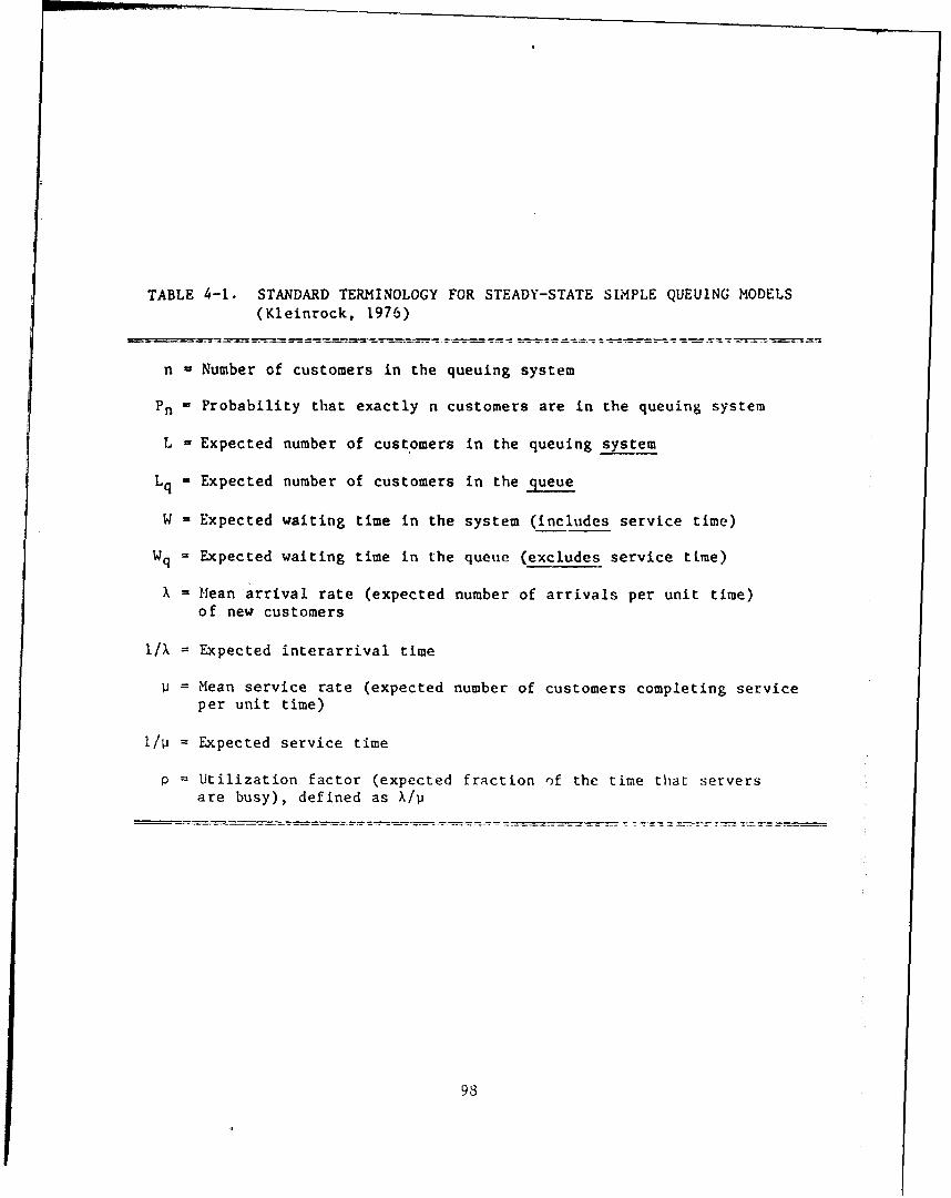
TABLE 4-I. STANDARD TERMINOLOGY FOR STEADY-STATE SIMPLE QUEUING MODELS(Kleinrock, 1976)
n - Number of customers in the queuing system
Pn = Probability that exactly n customers are in the queuing system
L - Expected number of customers in the queuing system
Lq - Expected number of customers in the queue
W - Expected waiting time in the system (includes service time)
Wq = Expected waiting time in the queue (excludes service time)
X = Mean arrival rate (expected number of arrivals per unit time)of new customers
1/% = Expected interarrival time
P = Mean service rate (expected number of customers completing serviceper unit time)
I/P = Expected service time
p = Utilization factor (expected fraction of the time that serversare busy), defined as X/p
98

TABLE 4-2. FORMULAS FOR DESCRIBING THE QUZUING PROCESS
For a steady-state queuing process:
LX
and
Lq - X Wq
For a classical M/M/I queue:
X P
Ii -x 1-P
therefore,
L I
[May also be designated as:
1E(tb) = , the expected length of the busy period)
whereI -E(ti) = -, the expected length of time the server is idle;
i.e., the expected interarrival time.]
However,
W = Wq +
therefore,
W q P P(ý1 I p p1 -
2pand i~q
It can also be shown that:
Po = 1-p (the probability that the queue is empty)
99

Error Rate Models
In the simplest case, there is an error probabilty Pe(p) as a functionof p, defined as the probability that a task is incorrectly completed. In thesimple case, incorrectly completed tasks are not redone. In a more complexcase, the incorrectly completed tasks are redone. Consequently, for the morecomplex case, the rate A of tasks is defined as
I= )X+ X Pe
where X is the externally-imposed task arrival rate and the second term isdue to the feedback (i.e., redoing) of incorrectly completed tasks. Note thatsuch a "human" queue, in contrast to the classic M/M/l queue, will saturate
Abefore the utilization factor p " - is equal to 1. In fact, It can be shown
that the human saturates for p 1 - Pe(l) 4 1.
Of course, it is necessary to have an empirical database to deterTaine thefunction Pe(P), or even just a constant value of Pe- Moreover, the task forwhich a queuing model with errors is used must be such that task completioncan be characterized simply as correct or incorrect. Other formulations arepossible, such as distinguishing between errors of commission and errors ofomission (Schank and Abelson, 1977).
Errors of Commission. Errors of omission occur as a result of the relation-ship between capacity, mean arrival rate (x), and expected waiting time (W),as in Fig. 4-2a. For human operators, we suspect that the mechanism of errorgeneration also involves an attempt to adjust or "stretch" response capacity Csuch that waiting time W of a task does not exceed a criterion level. Then,as apparent capacity C increases (e.g., as in the uppermost horizontal dashedline in Fig. 4-2b), the rate of errors of commission cC (e.g., character sub-stitution, number inversion, types, etc.) should increase proportionately, inaccordance with Shannon's law for noisy communication channels. Specifically,for 1 < C, error rate eC can be made arbitrarily small by proper task design(i.e., "encoding"). But for a given task design, any attempt on the part ofthe human to increase his apparent capacity C will result in an increase inerror rate rC.
Errors of Omission. By adding a threshold parameter to the classical I/M/Imodel, we can predict errors of omission. Assume that if W for a given taskexceeds a threshold parameter T, then the task is omitted by the servingresource and we say that a "reneg" has occurred; i.e., the "customer" or taskcannot "wait" any longer than a threshold time W = - and "leaves" the queue.This rene!ýnj• rate is eqiuiva lent to the error rate for errors of omission, F0,such as missed keystroke, missed symbol, missed message, etc.
100

INFORMATIONOUTPUT RATE
PERFECT ERRORS OFSYSTEM OMISSION
(CO)
PHYSICALLYREALIZABLE
MAXIMUM - - - - SYSTEMCAPACITY ---------
MAXIMUM -- -- "ERROR-FREE
TRANSMISSION -RATE HUMAN
CAPACITY
INFORMATION INPUT RATE R-3"A
(a) Differences Between Perfect, Physical, and HumanInformation Handling (after Miller, 1978)
INFORMATIONOUTPUT RATE
ERRORS OFOMISSION
(CO)
MAXIMUM
CAPAC ITY . . ..PI-- -. ERRORS OF
"-. S COMMISSION
(CC)EFI'LCT IVE"- . ( c
TRANSMI SS IONiýATF
"". HUMANINPUT CAPACITYPAIL
O!YATION INPUT RATE R-3610A
"A[IIMPTS 10 i;,0O'l I'-,ASTER PFIULT IN MOVING THIS POINT UPWARDS;i.e., F'I.PR I-RORS Of- (IMISSION BUT MORE ERRORS OF COMMISSION.IOTAL ERROR RAlE RIMAINS CONSTANT.
(b) Effect of Human Attempts to Process Faster
Ftgure 4-2. Human Error and Workload - An Information-Theoretic Paradigm
101

Let T be scenario-determined "time available" for a task from queue entryto completion of service; and let I/ij be the "time required" for service.Then T must be greater than the service time l/v plus the waiting time W inorder to minimize reneging. That is, in the steady state,
T > (Wq + I/u)
If T is less than this value, reneging or errors of omission will occur atan increasingly high frequency.
The "slack time" S for a task Is the time available minus the time re-quired for the task. That is,
S - -1- 1/ ,1/X - 1/P
For a lower bound for this expression, we substitute for T from the fore-going expression to obtain:
S >•
Workload-Dependent Service Rate
Let us assume that the service rate depends on the utilization factor,
V V(p) •
Then the effective service rate ' for a given queue must be derived from theexpression
Note that an alternative assumption would be that the human's processing rateis a function of the actual backlog of tasks to be performed, rather thanaverage operator utilization.
Reneging
An additional consideration is the potential reneging of tasks, i.e.,tasks that are not completed by a certain deadline cannot be completed at all.
102

An example is a task (related to ballistic missile intercept) that cannot beperformed if the incoming weapon impacts its target. As discussed above, non-completion of tasks can be viewed as errors of omission, and reneging/errorrates predicted.
4.3.3 Functional and Data Requirements for Queuing Theory Approaches
Lessons Learned from the SIMCOPE Modeling Experience: Defining Queues
The analysis that was done on the SIMCOPE simulated missile warning
facility at AAMRL (see Vol. Il) provided experience for dealing with theissues, problems, and expected benefits of using queuing theory approaches todescribe and predict human performance. The primary technical issues that hadto be addressed for SIMCOPE (and for other similar operational environments)are the following:
I. What is the ippropriate level of abstraction for describinghuman/system processes?
2. If a queuing (network) representation is to be used, what isit that will be queued and serviced? (viz., data, information,physical objects, or tasks?)
In dealing with (1) above, it has been assumed that IAT structural mod-eling must be taken down to a level of detail sufficient for identifying ele-mental tasks. At this level, measures of performance (MOPs) can be associatedwith specific processes that particular individuals carry out and for whichthey are responsible. Although measures may well be associated with higherlevels of analysis (in aggregated form), the raw data about human performanceshould be collected at the tasking level.
Question (2) then must be considered. One option is to let tasks bequeued to a human operator (or other resource) and serviced. This approachwas not taken in modeling SIMCOPE for the reasons listed below:
I. Strict definitions of "tasks" are not easy to formulate.*
2. Completing a task might require several decisions and/or actionson the part of the operator, and these might be difficult orimpossible to observe.
3. The procedural controls placed on an operator make task queuestroublesome to describe.
*However, it is possible to provide a formal description of the level at whichtasks cani be meaningfully identified. Set theory notation can be used tospecify appropriate level(s) of detail, as nart of the IAT recursive decom-position te'chnique described in Section 2.
103

Specifically, if tasks in the SIMCOPE example were comprised of message-handling processes (acknowledging, assigning, and filling out reports), itwould have been very difficult to place these tasks in a single queue -- oreven parallel queues based on separate task streams. The source of the prob-lem lies in the interrelations among tasks. Even for the relatively simpleenvironment in SIMCOPE, the number of interrelated tasks was large. Forreal-world systems, the situation is aggravated.
Another option, and the one that was taken in modeling SIMCOPE, requiresthat queues be defined in terms of physical entities (IAT RESOURCES). Thenthe processes necessary to service the items in the queue can be consideredin a more straightforward manner. The chief merit of this approach is thatit places the source of the demand for service with items which are easilyidentified and quantified -- rather than with tasks which may be somewhat moreopen to interpretation.
One consequence of defining queues in terms of RESOURCES is that a dataflow analysis identifies such queues directly. Moreover, any situation whereitems are filed (or stored) in anticipation of further processing suggests aqueue. Hence, there is no need to define tasks exhaustively before identify-ing queues. Another advantage to this approach is that measurement issues anddata collection become simplified: queues are based on observable physicalitems and events, as opposed to perceptual or cognitive ones. This last pointbecomes critical when descriptions of the system (such as the classified/unclassified documents on NORAD MWC and CP) do not contain service time datafor macroscopically defined tasks. This was the situation in SIMCOPE andwould appear to be the case for the NORAD MWC Validation Effort as well.
It is essential therefore that data necessary to support or validate thequeuing theory approach be directly observable or capable of being derivedeasily.
Defining Queue Discipline
An independent reason for using resources to comprise queues comes fromexamining problems associated with defining queue discipline. In the caseof a human operator (or any resource), goals and procedures will define whattask should be performed in a given circumstance. A task analysis should thenidentify the data used by the operator, as well as those processes the oper-ator carries out to complete the task. This type of analysis will definethe queue discipline albeit indirectly, but the description will be a naturalone from the prospective of depicting human performance.*
*This approach was illustrated in the SIMCOPE example via the overall data
flow diagram and the estimation of effective processing times. The diagramidentified services or tasks performed by the operator while the servicetime estimates were dependent upon the assumptions about the order ofprocessing and interruptions.
104

4.3.4 Recommendations for Using queuing Theory to Evaluate Human/System
Performance
I. View the human operator as a server for one or more queues.
2. Define thesc queues by tangible (observalle and measurable)items in the system. (!AT RESOURCES)
3. Use a data flow df:scription (e.g., with DFDs) to facilitateidentifying queues and major processes. (This will allow thequeuing network to be described with a minimum of abstraction.)
4. Make explicit the control structure of the system. (This isespecially important for cases in which one operator or resourceservices more than one process. A description of the systemcontrol structure would establish the order in which processesare to be performed.)
5. Use Petri nets to specify control structures.
6. Carry out further analysis (process modeling) to estimateservice rates:
a. Identify processes shown on the lowest-levels of DFDs.These processes are the appropriate ones for completinga given task, according to the conventions of data flowmethodology.
b. Determine completion times for each process identifiedin 6a).
c. Estimate conditional task completion times ("conditional"in the sense that full attention is assumed to be devotedto the task).
Levels of Detail
The SIMCOPE example and other experience suggests that while some of theimpact of system connectivity and structure on human function allocation couldbe analyzed at higher levels of aggregation, the level of process descriptiondefined in Gruesbeck et Al. (1984) was not sufficiently detailed to derivethe quantitative data necessary for performance analysis. Further decomposi-tion must be performed and data must be extracted by considering proceduresand system specifics (e.g., cued versus non-cued display, etc.). Such dataare obtained only after fairly detailed task analysis is completed. The de-composition should push down to the point of revealing generic processes suchas button-pushes and extraction of single items of data. This will insurethat analysts can use information from the human factors literature to fill
105

data voids in system-specific documentation. By working back up through theprocess description, the necessary service time data can then be estimated.
While gross trial allocations of functions can be performed at higherlevels of aggregation, only if given sufficient detail is it possinle to linkhuman factors design issues and data into a queuing network representationfor predicting performance. Without. going to this point, it is not clear thatsuch linkage can be achieved except in a purely empirical way (i.e., by esti-mating parameter values from observations of the system in operation). Also,it is only at this level that operator interface design and redesign issuescan be addressed.
Addressing Issues of Accuracy and Error
As illustrated in the SIMCOPE analysis in subsection 4.3.3, error ratescan be established by the task or service description. To use this approach,the process description must be sufficiently detailed so as to describe error-checking, editing, and various exit conditions* in a probabilistic manner.Service times will then directly reflect error by means of checking and correc-tion loops: these will have the effect of increasing average service times.Problem simplification strategies and load shedding could also be built intothe detailed process description, if desired, by making the processing activitys tate-determined.
4.4 STAPN4 MODTI N(
In Section 3 and Arpendix A a detailed basis for STAPN modeling of C3
systems, including humans, are provided. However, there are certain 1inimumdata requirements for using Petri nets which bear repeating at this F.tint.
4.4.1 Summary of Basic Data Requirements
To describe a model of PROCESSES, from which measures of performa,c(MOPs) and measures of effectiveness (MOEs) may be cuonputed, aL least tloefollowing is necessary:
I. A list of all of the places.
2. A list of all of t),2 branches.
3. A list of all of the transitions.
*e.g., -- Task completed error-frte
-- Task completed with one error-- Task completed with ritilr.iple errorse t C.
106

4. For each place:
a. A description of the process by which unavailable tokensare made available.
b. The transitions which insert tokens into the place.
c. The branch which describes where tokens go after theyleave the place.
d. The number of tokens iniLially in each place.
5. For each branch:
a. A description of the decision rule which selects the path
each token will follow.
b. The pl.ac-e, from which tokens exit through the branch.
c. The transitions to which tokens may flow (i.e., thealternative paths leaving the branch).
6. For each transition:
a. The places which must contain available tokens for thetransition to fire.
b. The places which receive unavailable tokens when thetransition fires.
These requirements can be grouped into three classes:
1. Decision rules (5a)
2. Timing data (0a)
3. Network topology (all others).
These form three hasic "dimensions" of the physical process toodel.
4.4.2 Metrics for Insuring Model Quality
One of the mrajor outputs of an IAT analysis is a physical process modelf rom which perforinance rnea.sures will he caiculate,.d. At least four desiderataapply tu tic outJL.,t of any such nethodology:
1. C.j.Inssl-t.!ncy: Is thc node]. (formally) well-structured! Area 11 comnccLions iei;d] ?
2. Completent U [ : Is; the mfod,'I f inished? Are there, •any l oose ends
-th-at-- d-- t be f1llf-d In?
I0j1
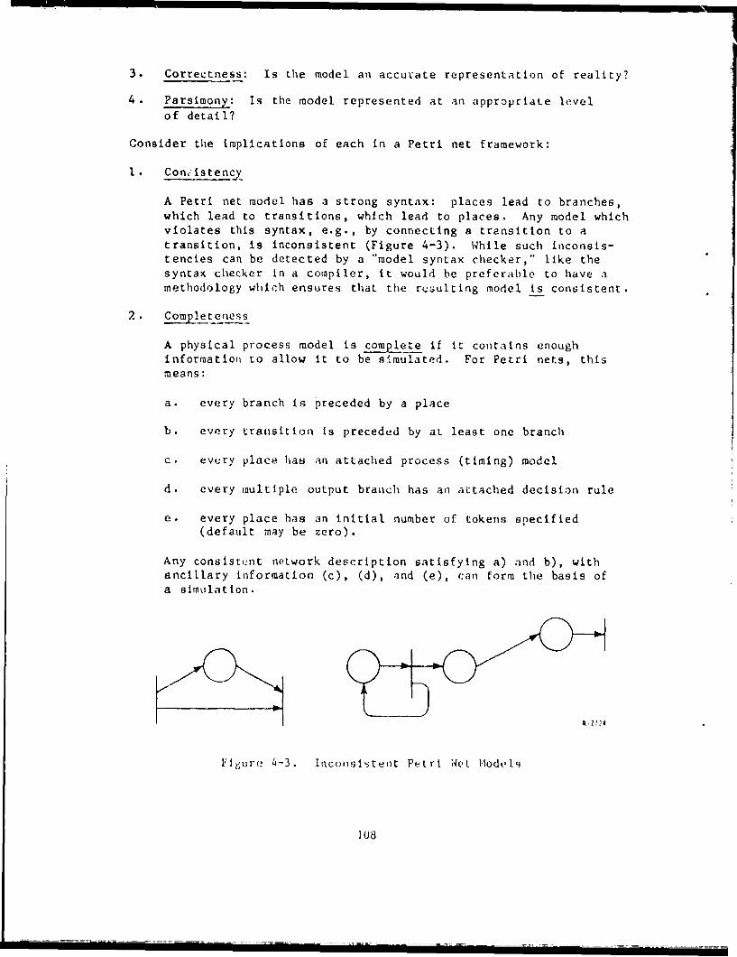
3. Correctness: Is the model an accu'ate representation of reality?
4. Parsimony: Is the model represented at an appropriate levelof detail?
Consider the implications of each in a Petri net framework:
1. Conistency
A Pertri net model has a strong syntax: places lead to branches,which lead to transitions, which lead to places. Any model whichviolates this syntax, e.g., by connecting a transition to atransition, is inconsistent (Figure 4-3). While such inconsis-tencies can be detected by a "model syntax checker," like thesyntax checker In a compiler, it would be preferable to have amethodology which ensures that the resulting model is consistent.
2. Completeness
A physical process model is complete if it contains enoughinformatioti to allow it to be simulated. For Petri nets, thismeans:
a. every branch is preceded by a place
b. every transition is preceded by at least one branch
c. evry place has an attached process (timing) model
d. every multiple output branch has an attached decision rule
e. every place has an initial number of tokens specified(default may be zero).
Any consistent network description satisfying a) and b), withancillary information (c), (d), and (e), can form the basis ofa simulation.
Flgure 4-3. Inconsisitent Petri Wet, Models
108

R-2725
Figure 4-4. Incomplete Petri Net Models
3. Correctness
Unlike consistency and completeness, correctness cannot beassessed just by examination of the model. The usual issues
of validation, etc. cannot be avoided. However, there aresymptoms of incorrectness which should be double-checked when
found:
a. A place with no inputs and no initial tokens isentirely superfluous.
b. A place with no inputs and some initial tokens isof transient importance only.
c. A transition which can never be enabled is superfluous.
Related to these symptoms, "liveness" (related to c)) and"boundedness" (no place where an infinite number of tokens canaccumulate) have been extensively studied in the literature.Dead or unbounded Petri nets may be incorrect models, or may
be correct models of improperly designed systems.
R-2722
Figure 4-5. Incorrect Model: "Vead"
1U9

R-2723
Figure 4-6. Incorrect Model: "Unbounded
4. Parsimony
This is an aesthetic quality. Theze is a fandamental tradeoffbetween the complexity of processes and decision rules and the
complexity of the network.
4.4.3 Extensions for Enhancing Model. Clarity and Completeness
I. Annotations - text commentary indicating the relationbhip of amodel element to the actual system.
2. Token Typing - labels oln tokens to describe the function/object/data they represent.
3. Multilevel Representations - aggregation of the process, proLo-col, and timing information into higher-level constructs (whichperhaps have non-local dependencies),
4. Other Dimren3ions - physical equipment models (from which timinginformation can he derived), organization/goal models (fromwhich protocols can be derived), etc.
4.4.4 Summary
In summary, Petri net process modeting can be complhoely described by Lheitems in subsection 4.4.1 plus
I. An annotation describilg the- facility or resource that tLhplace represents.
2. An annotation describing the purpose or .oa] of the brai;i'h.
110

3. An annotation describing the event modeled by the transition,
including uncertainty, timing, andT dependency relationships.
4. For each token type,
a. An annotation describing what the token represents.
b. The transition(s) at which the type is created.
c. The transition(s) at which the type Is destroyed.
5. As appropriate, aggregate models and token typing hierarchies.

112
SECTION 5
CONCLUSIONS AND RECOMMENDATIONS
5.1 CONCLUSIONS
While numerous system representation methods such as IDEFo, Data FlowDiagrams, and the SAINT and other simulation languages have long been avail-able, none of these techniques, either alone or in combination, could meetthe IAT requirements noted in Section 2. The main obstacle was the lack ofa single, underlying, integrating analytical framework (i.e., a theory of C3 ).With the development of the Stochastic, Timed, Attributed Petri Net STAPN)representation technique for manned C3 systems, this obstacle has now beenlargely overcome.
The results of the work to date have served to demonstrate the feasi-bility of IAT. Not only has the required analytical framework for IAT beendeveloped, but the following additional results have also been achieved:
- a mathematically rigorous symbolic language (STAPNs) for describing(i.e., modeling) and evaluating (i.e., assessing the system per-formance and/or military effectiveness of) manned C3 systems andtheir associated weapon systems at any level of description ordecomposition.
- a convenient means for managing system complexity by aggregatingand modularizing system details in the new Petri net "Box Node"aggregation prmitive, without masking the impact of these detailson overall system performance and effectiveness.
- a set of nested and self-consistent system measures derived fromthe symbolic language.
- a flexible data management system concept based on the artificialintelligence concept of frames and slots.
- computer-based instantiations of all of the above.
In Sections 3 and 4 it has been shown that classical analysis methodssuch as PERT/CPM and queuing theory, as well as computer simulation methods,can be made ani integral part of the STAPN methodology for IAT.
113

5.2 RECOMMENDATIONS
Based on the lessons learned from the three trial applications discussedin Vol. II, it Is felt that an automated aid to IAT must be developed with thefollowing features:
I. A "Friendly Front End (FFE)" to help the analyst describe anddecompose a C3 system using a "standard" graphic Input languageof his or her choice. Specifically:
- An analyst must be able to "enter" IAT using familiar oreasily learned, graphics-based techniques such as DataFlow or IDEFO Diagrams, and the FFE taust interactivelyassist the analyst in generating, decomposing, storingand accessing these diagrams.
- The FFE must incorporate a "Data Stripper" or means forautomatically stripping off from the stored Data Flowand IDEFo Diagrams the connectivity, information flow,dependency, control, resource assignment, and etherdata required to convert it into a STAPN model.
- The FFE must also incorpor.te a "Data Checker" to helpthe analyst build the required database. The mathemat-ical rigor of the STAPN modeling method autowaticallyprovides a "model" of the relationships among thevarious data elements, thus greatly reducing the diffi-culty of Data Checker development. The Vata Checkermust work interactively with the analyst to flag missingand/or inconsistent data and connectivities, and mustalso help generate a list of C 3 resources and theirassignments to C3 processes.
2. A database system organized around the Frame/Slot concept ofartificial intelligence to provide the flexibility needed tomake possible the features described herein. Data organizationis crucial to the success of an automated aid to IAT. The datamust be organized dimensionally and hierarchically to reflect thedecomposition levels within and among each of the four descrip-tive dimensions (Process, Resource, Organization, and Goal).For example, slots in a given process frame must be capable ofbeing used as "pointers" to associated processes, to assignedresources, to organizational assignments, to assigned perfor-mance goals, and to associated sets of measures (e.g., "PROD"statistics) contained in other frames, while maintaining con-sistency of description among the dimensions at a given decom-position level. To reduce the effort involved, the systemshould also contain a "default" database of key C 3 system andhuman operator/decisionmaker parameters. This will permitsensitivity analyses to be performed to determine which dataItem values require further ref inement (e.g., by ueans o0 man-in-the-loop exppriments).
114

3. An "Explainer" for explaining to the analyst why certain datainputs were required, why the structure of a STAPN model wasincomplete or inconsistent, and why selected MOPs and MOEs wereobtained when the model was exercised. Without such a feature,we hav. found that analysts will be loathe to use the automatedaids described above, and their "customers" will question thecredibility of their results.
Fortunately, except for the Data Stripper, many of these features havealready been or are in process of being developed for other projects, andneed only to be combined and integrated to form an automated analyst's aidto applying IAT. It is recommended that this be done.
i i ..... ii ir " - f = V-I

116

APPENDIX A
MATHEMATICAL FORMALISM FOR STAPNs
A.1 INTRODUCTION
In this appendix we present details of Stochastic, Timed, AttributedPetri Nets (STAPNs). The canonical Petri net variables and their relation-ships are Identified along with methods for both their decomposition andaggregation. Techniques for evaluation of measures are briefly described(detailed exam, - will be found In Volume I1), and Appendix A endswith a descriplioit of some of the systems analysis issues that have not yetbeen addressed.
A.2 CANONICAL MEASURES: PROD STATISTICS
In subsection 3.4 we established tight connections between the realityof a C3 system and the structure of an abstract STAPN representation of thatsystem. Given these high fidelity relations, conclusions drawn from theSTAPNs carry over directly to analogous statements about reality. In partic-ular, this section explains how the STAPN primitives give us a way to identifycanonical variables which describe their behavior, and henceforth we take forgranted the fact that these variables apply equally well to a real system.Appendix C contains procedures and guidelines for generating measures fromSTAPNs.
There are four types of canonical measures, each associated with a dif-ferent element of a STAPN: arcs, transitions, places, and tokens. There Isno distinction between capability measures, mission measures, or effectivenessmeasures: each of the four canonical types can play any of the three func-tional roles. In order to prod one's memory about the forms of the canonicalmeasures, we consider them in mnemonic order (yrobabilities, rates, occupan-cies, and delays), and do not distinguish between roles.
Before introducing the canonical variables themselves, two technicalaspects of their defiut~tions must be settled. First, some basic stochasticprocesses associated with STAPNs are introduced, processes that will form thebasis of explicit evaluation mechanisms alluded to in Assertion 4 on page 60.Second, each basic measure may be defined in four different ways, depending onthe evaluation mechanism used.
117

A.2.1 Basic Processes
Begin by considering any arc Ai in a STAPN. Suppose the STAPN's opera-tion is started several times, each execution called a replication of theprocess. For each replication, observe the tokens that flow along Ai. Thesetokens flow instantaneously and in sequence (ties may be broken arbitrarily toestablish a total order on the tokens that follow Ai). Let ti (n, k) be thetime (according to some external, global clock) that the n-th token traversesAi during the k-th replication of the STAPN operation. The ti (n, k) form aset of random variables which characterize much of the STAPN's behavior.
To derive measures from the qi (n, k), for each arc Ai and each replica-tion k, define an indicator function Ii (t, k):
ji (t, k) - En 6 (t, ti (n, k))
where the sum is taken over the total number of tokens passing over Ai in thecourse of replication k. The 6 (., .) function is the Dirac delta: a func-tion which is zero almost everywhere and which integrates to unity when thevalue of one argument is included in the range of integration of the other.
The Ii (t, k) are the most basic stochastic processes for a STAPN. How-ever, more important is the counting process Ji (t, k), which gives the numberof tokens having traveled on Ai between time 0 and time t, in replication k.Ji (t, k) is related to Ii (t, k) by:
tJi (t, k) =f Ii (s, Q) ds
0
The processes Ii (t, k) and Ji (t, k) are the primitive stochasticprocesses from which the canonical measures will be constructed. Note thatthe algorithm for generating either of these two processes from observationsof a STAPN's behavior is consistent with Assertion 4.
A.2.2 Forms of Measures
To see the differences between four forms of measures, consider Ji, thenumber of tokens having passed over arc Ai, as an example measure. This basicquantity can be interpreted as an instantaneous value; it may be averaged overa number of replications, over time, or both; the averages may be finite orinfinite.
An instantaneous value of a measure is taken at one instant of time t ina single replication k. To make this dependence explicit, denote the instan-taneous value of Ji as Ji (t, k), as above. Since tokens are almost never onarcs, Ji (t, k) is piecewise constant, with unit step discontinuities at acountable number of values of t and k.
118

An ensemble averaAge is taken over several replications. Denoted by theform Ji (t), ensemble averages may be computed from the instantaneous valuesas:
Ji (t) = K- Ek Ji (t, k)
where K is the number of replications. Unless K is explicitly mentioned,sssume K is infinite:
J Wt = limK+-, {K-1 E Ji (t, kQ1
A time average is, of course, taken over time. Time average measuresare denoted by the form Ji (k), preserving the dependence on the replicationindex. Time averages may be computed from the instantaneous values as:
TJi (k) =T-1 f Ji (t, k)
0
where T is the time interval of interest. Note that Ji (k) takes on theinterpretation of a rate: the number of tokens which cross Ai per unit time.Again, unless T is explicitly specified, assume T is infinite:
TJi Mk = limT+- IT-' f ii (t, k)1
0
If this limit exists, and the system does not exhibit periodic behavior, thenJi (k) is often refered to as a steady state measure.
Finally, a time-ensemble averaje is, as expected, taken over both timeand replications. These measures are denoted by the form Ji, suppressing thedependence on time or replication index. These averages may be computed fromany of the above in the obvious ways. Both averages are assumed infiniteunless stated otherwise.
Which of these four forms is preferable? The answer depends on the usesto which they are to be put. Instantaneous values or ensemble averages areuseful when the situation or system structure changes over time, since theyare applicable at every instant of time. Time averages are useful when thesystem and its environment are in some sort of equilibrium, so that a steadystate measure can be considered meaningful.
In subsequent subsections, only infinite ensemble averages and infiniteensemble-time averages (steady state measures) will be considered (e.g., ii (t)and Ji). Definitions of canorical measures given in these forms can readilybe adjusted to provide definitions of the measures in the other forms. How-ever, if finite averages are used as measures, the limits of the averages(i.e., K or T) musct be specified in order for the measures to be well defined.
119

A.2.3 Probabilities
The first canonical measures are associated with arcs leaving places.To each place corresponds a decision rule, which specifies by which arc eachtoken departs. A certain fraction of the tokens that leave the place followeach of the exit arcs; these fractions are the canonical probability measures.
Formally, suppose place Pi has output arcs A,, A2 , ... , AK. Define the Kprobability measures associated with those arcs as:
Given that a token leaves place i at time t in some reylication,th_._ rab y h the token leaves on arc n is:
Pin (t) = Il (t) / Tk 1k (t)
The stead state robabilit that a token leaves lace ± via
arc n is:
Pin = limt+. {Jn (t) / Ek Jk (t)}
Since Pin (t) is defined only at a countable number of points (since only acountable number of tokens are generated 4-n a countable number of replica-tions), care must be taken in the determination of the time average Pin. Tokeep Oin dimensionless, we take the definition of Pin as an assertion, not adirect consequence of the definition of Pin (t).
All of the probabilities are unconditional probabilities. their defini-tion assumes nothing is known about the activities in other parts of a net.Conditioning the probabilities on such knowledge can drastically change theirvalues. For example, consider the partial net (Fig. A-i). Without knowledge
P P 4TPP
P3
P2 C - P5
T2
Figure A-I. Conditinal Exit From a Place
120

of the placement of tokens in P1 and P2 , P31 and P32 might both be, say, 0.5.However, conditioned on the marking of the net in Fig. A-i, the probabilitythat the token in P3 leaves through T1 is 1.0. Thus a probability measure Pikmust be carefully interpreted; it is meaningful and well defined preciselywhen the only knowledge about the net is that some token is leaving place i.
Every place has at least one output arc, so at least one probability mea-sure is defined for each place. If exactly one output arc leaves a place, thevalue of the probability measure for that arc will always be 1.0, irrespectiveof any other structure or activities of the net. This is a degenerate exampleof a canonical measure, and formally defined but rather useless in practice.
A.2.4 Rates
The second canonical measures are attached to transitions. Transitionsfire; this is their essential activity. In most STAPNs, transitions firerepeatedly, and it is meaningful to measure how often they fire. The fre-quencies with which transitions fire are called the canonical rate measures.
Formally, suppose transition Ti has input arcs Al, A2 , ... , Ay and outputarcs AK+I, AK+2, ... , AK+L. Due to the coordination role of transitions, andthe fact that exactly one token passes over each and every one of these arcswhen Ti fires, it is known that:
Jl (t) = J2 (t) in... =JK+L (t)
Without loss of generality, Jl (t) can be used in the definition of the canon-ical rate measure for transition TI:
The rate at which transition i fires is:
Xi (t) = d/dt [ Jl (t) ]
The steady state firin4 rate of transition iiLf it exists,_.is:
The firing rate of a transition implies that tokens flow along each ofits input arcs and output arcs at exactly the same rate. From these, tokenflow rates into and out of a place can be determined by summing arc flow ratesover all input or output arcs of that place. Because of these relations, ratemeasures need not be defined for other elements of a STAPN.
121

A.2.5 Occupancies
The third canonical measures are connected with places. Places storetokens between their creation and destruction. The natural quantities toassociate with places are the number of tokens which occupy those places;these are the canonical occupancy measures.
Formally, suppose place Pi has K input arcs labeled AI, A2 , ... , AK and Moutput arcs AK+l, AK+2, ... , AK+M. Tokens arrive in the place over any Inputarc, so the process which Indicates the total number of arrivals into tieplace, by time t, is
Ek Jk (t)
Similarly, the process which indicates the total number of departures from thesame place, by time t, is
Em JK+m (t)
Now, the number of tokens in the place at tIme t is some initial numaber oftokens specified by the marking of the STAPN, ni (0), plus the number thathave arrived, less the number that have departed:
The occ.uýan nc_ ofy _Lace I s :
l (t) - ni (0) + Ek Jk (t) - Em JK+m (t)
The steady state occupdncy of place i it it exists. is:
T
ni - ni (0) + limT,' I r-l f rk -)k (t) - Em JK+m (t) dt0
A.2.6 DelaJs
The fourth canonical measures apply to tokens. Tokens exist betweentheir creation at one transition and their destruction at another. Thenatural quantities to associate with tokens are their lifetimes; these arethe canonical delayn measures.
Formally, consider all tokens created in place Pi and destroyed by outputtransition Tj. (All such tokens spend their lives in the same place. How-ever, different timing models may describe the duration of their unavailablestate, since they may have been created by different transitions.) N4umberthese tokens in order of their creation, ustng the index nij to emphasize thedependence on both P1 and Tj. Let ti (nij, k) be the time of creation of thenij-ti, token to arrive at Pi in replication k; let tj (nij, k) be its tirie of
122

destruction at T-. Note that delay measures are defined on a token by tokenbasis, so we rausi replace time averages with token averages to form steadystate measures:
The delay exper encedbefore time tb tokens between arrival
.ljkace I and dsrcinat transition is
Tij (nij) = tj (nij) - ti (nij)
The steady state delay experienced by tokens between arrival at place i anddestruction at transition j, if it exists, is:
Tij " limN+- I N-I En rij (n) }
Note that tij (nij, k) is defined only when the ni -th token from Ti to Tj hasbeen destroyed, t at is, when tj (nij, k) is known. Tokens which have beencreated, but are still in a place, do not have a permanently defined lifetimeand are thus excluded from this definition. Tokens which are part of theinitial marking arrive at their respective places at time 0, when the STAPNstarts to operate.
Finally, note that these delays are conditional delays: they representthe time a token spends in Pi given that it exits through Tj. They do notdescribe the delay which any token experience: in Pi, although the lattermeasure can be computed from the canonical delays and probabilities.
A.3 HORIZONTAL RELATIONS BETWEEN MEASURES
From the dincussions above, it is clear that not all measures are indepen-dent. The most trivial example occurred in the case where a place has a sin-gle output arc: the probability for that arc is 1.0, regardless of anythingelse. This section identifies four classes of relations which exist betweenthe canonical measures of a STAPN.
Consider the partial STAPN and its canonical measures in Fig. A-2. Anumber of relationships hold between the measures shown here. For example,equations which relate the steady state measures happen to be:
P12 + P13 = 1.0 Conservation of probability
Xi= X2 + X3 Conservation of rate
X2- P12 * X1 Probability -- rate relation
X3 P13 X Probability -- rate relation
xI=1 * (P12 -112 + P13 * T13) Occupancy -- rate -- delay relation
123

T 2
P 2
12
1 13
13
rigure A-2. Canonical Measures
The four types of relations exemplified above can be generalized; infact, similar equations exist for the steady state measures surrounding everyplace in a STAPN. For measures expressed as ensemble averages, the analogousequations are not algebraic; they take the form of delay-differential equa-tions (which cza be viewed as relations between entire time functlons, ratherthan between single values). Whatever the form, these equations jrov4 de theset of horizontal relations that apply within a single STAIPN model.
A.3.1 Conservation of Probabilityj
Recall that thb canonical probabilities measure the fraction of tokensthat leave a place along each of its exit arcs. Since every token that leavesa place must follow exactly one output arc, these fractions must sum to one.
Formally, suppose place Pj has output arcs A,, A2 , ... , AK. The firsthorizontal relation between measures is:
Conservation of Probability:For ensemble avere:
Ek Pik (t) - 1.0
For sready state statistics:
Ek Plk = 1.0
124

These relations imply that one probability measure at every place is redundant--including the trivial situation where only one arc leaves a place.
A.3.2 Conservation of Rates
The second class of horizontal relations also follows from the fact thattokens do not evaporate from places. Every token that enters a place eitherstays there, or leaves to be destroyed at a transition. As long as tokens donot pile up in a place indefinitely, the sum of the output rates must approachthe sum of the input rates.
Formally, suppose a place Pi has K input arcs labeled Al, A2 , ... , AKfrom transitions T1 , T2 , ... , TK respectively, and M output arcs labeled AK+I,AK+2, ... , AK+M to transitions TK+I, TK+2, ... , TK+M. Recall the basicoccupancy equation:
fli (t) = nI (0) + Ek Jk (t) - Em JK+m (t)
Differentiating both sides with respect to time, and substituting the defini-tions of rate statistics provides:
Conservation of Rates:For ensemble avera!es:
d/dt rn[ (t) = Ek Xk (t) - Em XK+m (t)
Em XK+m (t) = Ek Xk (t) - d/dt nj (t)
For steady state statistics,- if they and ni exist:
Em XK+m = Ek Xk (t)
These relations imply that many rate statistics are redundant. The STAPNtopology restricts the channels which tokens may follow; tokens that contri-bute to a rate statistic at the input to a place must eventually contributeto an output rate at the same place.
A.3.2 Probabil it_ Rae _latRions
The third clav;s of horizontal relations results from the process whichdetermince how a tokcn departs from a place. The total flow of tokens into a
125

place diverges into flows along each output arc, so that the total flow outof the place is the sum of the output transition firing rates. A probabilitydescribes the fraction of that flow which travels along each arc, and the flowalong each arc equals the firing rate of the transition terminating that arc.Thus we can relate individual output transition firing rates to the totaloutput firing rate.
Formally, again suppose a place Pi has 1 outpuL arcs labeled Al, A2 , ... ,
Am to transitions Tl, T2 , ... , TM respectively. From the definItion of C1u (t):
In (t) = ym Im (t) * Pn (t)
Note that
d/dt Jn (t) - limK+m I K-I Zk d/dt Jn (t, k)
so
An (t) Ii= imK { K-I1 k Im (t, k) In (t)
Similar manipulations apply to the steady state sttitiSLcs. From the defini-tion of Pn:
limT+, { T-1 Jn (T) } lim T- M Jm (T) *
and passing to the !imit:
Xn = { X, 1 xnP1
These arguments give us the third kind of horizontal relation:
Probability-Rate Relations:For ensemble aver_1_:
An (t) = Fm Xm (t) * Pn (t)
For steafdy state statisticsL.ifthey exist:
An = .n Am * Pn
126

These relations can be used two ways. If canonical probabilities are known,then all rates for the output transitions of a place can be deduced from anyone such firing rate. If all rates are known, then we can solve for allprobabilities without any other information.
A. 3.4 Occu pancy-Rate-Delay Re I ations
The final class of horizontal relations exploit two different interpreta-tions of the same quantity: the number of token-seconds spent in a place.This can be computed by adding up the lifetimes of all tokens that transit aplace, or by integrating the number of tokens present over time.
Formally, suppose a place Pi has K input arcs labeled Al, A2 , ... , AKfrom transitions TE, T2 , ... , TK respectively, and M output arcs labeled AK+1,AK+2, ... , AK+M to transitions TK+I, TK+2, ... , TK+M. Consider the nth tokenthat passes through Pi, departing through TK+m at time
t = tK+m (n)
At this time, the total number of tokens having passed through Pi is
Em JK+m (t)
Assuming first-in, first-out passage of tokens through Pi, this n-th tokenwill have arrived at Pi at some time t - Ti which satisfies:
Ek Jk (t - Ti) = rm JK+m (t)
Differentiating both sides with respect to t(n),
Ek Xk (t - i) * (I - d/dt Ti) = Im XyK+m (t)
Rearranging terms, the delay encountered by a token leaving Pi at time t isTi, given by the delay-differential, equation:
d/dt { Ek Xk (t - Ti) - Tm 'K+in (t) } / Ek Xk (t - Ti)
Now consider the steady state statistics. The total amount of time spentby those tokens in Pi, which have left via TK+m by time t, is:
127

81,K+m (t) = Sn ti,K+m (n, t)
The total amount of time spent by all tokens in Pj which have left by time tis:
i (t) = EZ 0 1,K+m (t)
The number of tokens departing Pi by tLime t Is:
O0 JK+m (t)
so the average amount of time, per token, spent in Pi is:
eA (t) /4, JK+m (t)
Now, an alternative way to compute Oi (t) is:
t
0± (t) - f ni (t)0
Letting Ti be the average time any token spends in Pi, the combination of thelast two forms yields:
TI {T- 1 f ni (T) /{ T-1 EmJK+m (T)}
0
Passing to the limit in T gives Little's formula, well known from queuingtheory:
Ti = Ili / Em ýK+m
These arguments give us:
Occupan.jy -- Rate -- Delay Relations:For ensemble ave rae.s:
d/dtr = { Ek Xk (t - FI) - Im XK+m (t) } / Ek Xk (t - Tj)
128

For steady state statistics, if. they exist:
fli - Ti * Em XK+m
These equations are not quite complete, since they involve the uncondi-tional delay in Pi, namely Tt. Instead of applying just to tokens leaving Piby a specific arc, Ti is an average over all tokens passing through Pi, andhas not been seen before. Conditional delays, Tij, have been defined previ-ously, but are defined with respect to a specific transition T . Fortunate-ly, the two delays are easily related to one another. For ensemble averages,if the ni,K+m-th token departs Pi via TK+m at time t,
"Ci (t) = Ti,K+m (niK+m)
For steady state statistics, the unconditional delay ib simply a weightedaverage of the conditional delays:
Ti = Em Pi,K+m * Ti,K+m
A.3.5 Implications for Minimality
Clearly the entire set of canonical measures for a STAPN, while entirelymeaningful, includes redundant elements. The four types of horizontal rela-tionships described above apply to any STAPN, and thus can be used to elimi-nate redundant measures. By first identifying all canonical measures, thenfinding all of these horizontal relationships, one has a simple procedure foreliminating the redundant measures. Simply select one relationship, eliminateone measure which appears in it, use it to replace all occurrences of theeliminated measure in all other relations, then repeat for each other rela-tion. Of course, the equations above provide no gu'iance pertaining to theorder in which relationships and measures should be selected in this process.
The power of these relations can be clearly seep when steady state sta-tistics are used. For example, one can use the occupancy-rate-delay relationsto compute all occupancies from rates and delays, so all occupancy measurescan be eliminated. Then one can use the probability-rate relations to com-pute all probabilities from the rates, so all probabilities can be discarded.Finally, the conscrvdtion of rate relations eliminate a rate measure frota oneoutput transition of each place. By followinýg these steps, a majority of thecanonical measures can be removed from thi! original set of candidate measures.
There is w) guiar,,ntee that the canonical relations are the only sourcesof dependence j:monig measures. Indeed, when values of measures are to be com-puted, additionlal relations mu.:t be rnide available in order for the values to
129

be completely determined. The four classes of relations presented here are,however, the only relations which always hold and which may be determinedsolely from the topology of tha STAPN.
A.4 REFINEMENT OF MODELS
Petri net models of real systems are notoriously complex -- often pro-
hibitively so. In order to manage the unavoidable complexity of C3 systems,we have suggested that STAPN models could be arranged in hierarchlies, witheach level representing the same system but with differing amounts of detail.Well defined connections between models at successive levels allow the generalstructure depicted in a higher level model to be transferred to lower levelmodels. In addition, these same connections can help structure the modelbuilding process, and give rise to quantitative relations between measures atneighboring levels.
A.4.1 Disaggregation and Enhancement
Two mechanisms exist for expanding a model from one level of detail 1o
another, based on opposing philosophies. The first is strict structured decom-position or disaggregation, where each element of a level N model decomposesinto a set of elements at level N+l, and where the level N+l model containsnothing but these decomposed elements. We naturally think of disaggregationin terms of geographical regions, where nations disaggregate into nonover-lapping territories, and every acre of land is contained in some territory.Similarly, organizations often disaggregate from divisions to groups to peo-ple, and every person is a member of one group, every group is part of onedivision. Strict disaggregation is a powerful technique when it can be used,as it implies precise relationships (homomorphisms) between the structuralelements depicted in successive modeL -Levels.
Unfortunately, very few real systems can be disaggregated so that theirhigher levels are just 3ggregated versions of their lower levels. More often,the lower levels contain details that have no counterpart at the higherlevels. Yes, the United States can be disaggregated into fifty states andseveral territories, but where do national parklands and Indian reservationsfit into this scheme? Yes, organizations can be disaggregated into divisions,but where do interdivisional programs and matrix management fit in?
To deal with real C3 systems, we must be prepared to consider detailsrelevant to level N+l which do not appear at all in higher level models. Forexample, special purpose messages, which are part of a protocol to manage acommunications network, should be suppressed in any simple model of the missionwhich that network supports. Such details which appear afresh at level N+l,without being modeled at level N, are enhancements to the model of level N.
The distinction between disaggregation of a model, which implies strongrelations between models at two adjacent levels, and enhancement of thatmodel, which precludes any such relations, becomes pirticulurly ifportant
130

when we derive vertical relations between the measures associated with thetwo levels. Subsection A.4 will revisit this distinction; for now, we simplyexplore three techniques for increasing the detail of an existing model:two disaggregation methods (one for transitions and another for places) andenhancement.
A.4.2 Disaggregation at Transitions
The simplest disaggregation technique expands one transition at level Ninto several transitions at level N+I. This partitions the events (physicalboundary crossings) modeled by the higher level transition into subsets ofevents, one subset for each lower level transition.
Formally, consider two STAPN models of the same system, organized at twolevels of detail. The model at level N contains some transition TA, and themodel at level N+l has some transitions TB,I, TB,2, ... TB,M. Define:
Transitions TRI,_•,2, ... T ,K form a strict disaggregation oftransition TA if and only if there is a one-to-one correspondencebetween firings of the former and firings of the latter.
A simple illustration of disaggregation at a transition is shown in Fig. A-3.Here, transitions TB2 and T8 3 form a disaggregation of transition TA2. (To beprecise, this is the case if and only if TBI is a trivial disaggregation ofTAI, so every token entering PAl corresponds to a token entering PBI') Sincetokens may leave PAl only via TA 2 , and PBl only via TB2 or TB3, there is aone-to-one correspondence between firings of the shaded transitions in the twomodels.
T AI pB
Figure A-3. Disaggregation at a Transition
131

Physically, disaggregation at transitions divides the flow of objects ormessages across some boundary into component flows. The components may bedefined in two ways. First, a Ringle class of objects at the higher levelmay be divided into several clas:ies of objects at the lower level. For exam-ple, messages arriving at a facility may all be lumped together at the higherlevel, but broken out by type it the lower level. Secondly, the actual bound-ary may be refined, being broken into segments across which obJects of thesame type flow. For example, the flow of enemy helicopters across the forwardedge of the battle area can be decomposed by the sector from which they arrive.
In summary, disaggregation at transitions supports hierarchical decom-position of token classifications and of boundaries.
A.4.3 Disaggregation at Places
The second disaggregation technique expands one place at level N into severalplaces and transitions at level N+l. This refines the model of processingdone at a place in the higher level model into individual processing steps.
Formally, consider two STAPN models of the same system, organized at twolevels of detail. The model at level N contains some place PA, and the modelat level N+l has some places PB,I, PB,2, - PB,M" Define:
Places 1 , "'-PB, form a strict disaggregation of place PAif and only if there is a one-to-one correspondence between tokensin the former and in the latter.
A sim l- illustration of disaggregation at a place is shown in Fig. A-4. Here,places PCI, PC2 and PC3 form a disaggregation of place PBl- (Again, this isthe case if and only if each TC,m is a trivial disaggregation of transitionsTB,m, m = 1, 2, and 3, so every token entering PCI corresponds to a token en-tering PB1, and every token leaving PC2 or PC3 corresponds to a token leavingPBl') Note that the two processing paths in the original model (TB 1 to PBlto TB2, and TBI to PB1 to TB3) are each decomposed into a single sequence oftransitions and places in the lower model, but that the latter share TCI andPCI. Note also that the new transitions, TC4 and TC5, have no counterpartsin the original model, so they are not disaggregatior.s of any original tran-sitions. if the initial number of tokens in PCI, PC2 and PC3 equals the inl-tial nm, bhr of tokens in P 13, thei there will always be a one-to-one corrc-spondence between tokens in the shaded places of the two models.
Physically, disaggregation at places divides the processing of objects ormessages in a region or facility into processing substeps. For each pair ofinput and output transitions i:i the original model, a sequence (;:ore general-ly, an acyclic network) of places and transitions appears in the lower modelto convey details of the original processing. Just as tokens in the originalmodel share residence In the original place, so the refined processing path-ways may share traansitions and places. However, no coordination mechanismother than simple sequencing along each pathway is possible using place dis-aggregation, as more sophisticated coordination mechanisms require additionaltokens, usually to rupresent memory in the coordination mechanisia, which haveno counterparts in tCe original model.
1 3.;

T83
T Bi
TB2
/T
Figure A-4. Disaggregation at a Place
The natural physical candidates for place disaggregation are decomposi-
tion of regions into subregions, division of facilities into components, and
segmentation of procedures into steps. For examples, a high level model might
represent an entire nation with one place, using transitions between places
to model border crossing events; a lower level model might use a place foreach state or county, with additional transitions modeling internal border
crossings. The North Cheyenne Mountain Complex might be a single place in
one model; each operations center might be a place in a lower level model,with some additional transitions modeling message or personnel movement be-
tween centers. The launch preparation process for a strategic missile might
be captured by one place in a high level model; at a lower level, individual
places might represent separate preparatory processes such as fueling, arming,and targeting.
In summary, disaggregation at places supports hierarchical decomposition
of regions, facilities, and procedures.
A.4.4 Simultaneous Disaggregation/Subnetworks
Parenthetical comments following Figs. A-3 and A-4 indicated that simul-taneous disaggregation at both transitions and places is needed in order toassert that either one is valid. That is, one-to-one correspondences between
tokens can be maintained if and only if there exist one-to-one correspondencesbetween the events that create and destroy tokens (transition firings). Thus
procedures to validate that a place disaggregation is correct must introduce
compatible transition disaggregattons, and vice versa.
133

Formally, the correspondences between tokens and transition firings pro-vided by a simultaneous disaggregation provide a well defined homomorphismbetween two model levels. In subsection A.4, we will see that this homomor-phism creates exact relationships between measures at the two levels.
From a practical perspective, simultaneous disaggregation is more readilyunderstandable than artificially enforced separations between disaggregationat transitions and at places. In fact, simultaneous disaggreg.ition can beinterpreted quite naturally as subnetwork expansion. Each place is disaggre-gated into a subSTAPN, which may model the decision rule or timing model forthe original place in more detail. Each transition is disaggregated to ensurethat the boundaries of the subSTAPNs are compatible: the output transitionsfor one subSTAPN must match the input transitions of any subSTAPNs that followit. Thus simultaneous disaggregation permits construction of hierarchies ofmodels which have precise correspondences between elements at successivelevels.
A.4.5 Enhancement
However, simultaneous disaggregation is not sufficient to model real C 3
systems. The high level structure of these systems only becomes apparent whensome details are completely suppressed. We must have a method for resurrect-ing these details as the model levels become more detailed, or risk losingthe completeness property of the models. That method is enhancement: addingadditional STAPN primitives to a model for which no corresponding elementexists at the level above.
There is no formal definition of enhancement, but the concept is ade-quately illustrated by example. In Fig. A-4, we disaggregated a place intothree places and two transitions, but added no information about the decisionrule for the original place. Suppose that logic is to send alternating tokensto PC2 and PC3" The lower level model of Fig. A-4 can be enhanced to capturethis special coordination mechanism as 3hown (Fig. A-5). Here, tokens alter-nately occupy PD4 and PD5, thus enabling transition TD4 for every other tokenthat becomes available in PDI" However, there is no token at the higher levelthat corresponds to the token initially in PD5- (Similarly, no transitionsfire at the higher level when either TD4 or TD5 fire, as seen in Fig. A-4.)Thus PD4 and PD5 constitute an enhancement to the higher level model.
Physically, enhancement adds structure to a model. It does not nullifyany aspects of a higher level model, but introduces new objects and coordina-tion mechanisms to extend the detail of that model. For most simple STAPNmodels, complexity not represented by the network itself is hidden in the
decision rules and timing models. Thererore, we would expect enhancement to
inject more visibility into these elements as a model is refined.
Figure A-5 is a simple example of how an allocation decision rule, modeledsimply as the separation of two token flows in Fig. A-3, can be made explicit.
Similar mechanisms express the detai" of other common allocation rules, such
as allocating a message to an operator with the shortest queue. Timing models
134

T C P C3T C
T• PC ToC4 C2
TTT DD 3
TD4 PD2
Figure A-5. Enhancement
used in higher level models usually represent activities of long duration,
such as establishing the identity of an object, and a lower level enhancementwould make explicit the time taken when false identities are conjectured andrejected, perhaps several times, before the true identity is established.
Finally, we saw that disaggregation only pernits processes to be decom-
posed into sequential subprocesses. In order to introduce the parallelismand related coordination mechanisms so vital to C 3 systems, we cannot relyon disaggregation alone. Enhancement provides the opportunity to introduceparallel processing paths and additional coordination between them, as inFig. A-S.
In summary, enhancement supports hierarchical decomposition of decisionrules, timing models, and coordination mechanisms.
A.4.6 Implications for Completeness
in addition to the usual issues of model fidelity, internal complete-ness is i propertLy of hierarchies of models that can potentially be verified.
135

The disaggregation techniques provide the structure for validating internalcompleteness.
In what sense can one expect a hierarchy of models to be Internally com-plete? It has been repeatedly argued that much detail present in lower levelsmust be suppressed from higher levels for the models to be managable. Enhance-ment is a necessary technique for building hierarchical Aodels of C3 , so onecannot ask that all features present in one level be present in all levelsabove. One can, however, demand that nothing be lost as we work more detailinto the models -- i.e., that every object and event captured by a high levelmodel be included in some component of each lower level model.
In STAPN terminology, internal completeness demands that every tokencreated at level N have a unique counterpart at level N+l, N+2, ... , and thatevery transition firing at level N corresponds to a unique transition firingat every level below it. Suppose that:
Assertion A-1: Every STAPN model of a system can be decomposedLbsuccessive disaglregations (at either places or transitions) andenhancements.
Now, the properties required for strict disaggregation (one-to-one cor-respondences between tokens and transition firings at successive levels of themodel) are transitive (so that they apply between levels N and N+K+M If theyapply between levels N and N+K, and between levels N+K and N+M). Thus ifsuccessive disaggregation-enhancement steps are used to build a hierarchy ofmodels in a top-down fashion, any token or firing in level N will have aunique counterpart at every level below, so
Fact A-1: Every STAPN model constructed from top-down iterationsover disaggregation-enhancement ste s, where the disaggregation isperformed at every place and every transition. is internally__coplete.
Thus one can ensure internal completeness for a collection of STAPN models bycarefully structuring the model-building process, so that disaggregation andenhancement are alternated as the model Is built in a top-down fashion.
A.5 VERTICAL RELATIONS BETWEEN MEASURES: AGGREGATIUN
Suppose one has two versions of a model at different levels of detail,and they are related to one another as described in subsection A.4. How dothe connections between models carry uver :nto relationships among measi:res?
For each of the four types of canonical measure, the disaggregationmethods produce a set of vertical relations which determine values for thehigher level measures from lower level values. If the conditions of Fact A-Iare followed, one vertical relation is produced for each high level measure.Since the structures introduced by enhancement are not part of the disaggre-gations, the measures associated with the enhancement elements will not appearin any of the vertical relations for the level above.
136

A.5.1 Paths and Path Sets
We will use the same notation in the discussion of all four classes ofvertical measures. Any simultaneous disaggregation process starts with someplace at level A, PA, its input transitions TA l, TA,2, ... TAK, and itsoutput transitions TA,K+I, TA,K+2, ... , TA,K+M. Disaggregation at the inputtransitions produces transitions TBI, TB,2, ... TB,L at the next level B.Disaggregation at the output transitions produces transitions TBL+l, TBL+2,0.. TBL+N. Finally, disaggregation of PA,i produces several new places PB,I,PB,2, -' PB,J"
Common to several definitions of vertical relations is the notion ofa path set. A ath under A is an alternating sequence of transitions andplaces which (a) starts at one of the disaggregated input transitions TB,1,TB,2, ... TBDL, (b) terminates at one of the disaggregated output transitionsTB,L+l, TB L+2, ... TB L+N, (c) only contains a subset of PB 1, PB,2, •PB,J, and (d) is acyclic. The collection of all such paths Is the path setfor PA, denoted as SA. The collection of all paths In SA that terminate ontransitions diaggregated from TAI is denoted by the set SA,AI.
This definition of paths, along with the properties of the disaggrega-tions which produce them, resnlts in an essential characteristic of a path
se;If several pat hs connect .AIset. -fsvrlytscnetayone dis!ggregated input transition to any
disa.g[egated outut transiontheX diverge and converge only.at places.
The proof of this fact is by contradiction. Suppose two distinct pathsin a path set diverge at a transition. Suppose this transition, common toboth paths, fires. This creates one token in each of the two next places ofeach path. By the definition of place disaggregation, each of these two tok-ens must bear a one-to-one correspondence with tokens in the original, aggre-gated place. Since only one token is created in the aggregated place in theupper level model by this firing, these two tokens are In a one-to-one corre-spondence with the same token, thus producing a contradiction. The proof forconvergence at places is proven by the same arguments, working backwards intime from the disaggregated output transition.
There may be several paths containing any single place. For example,consider the higher level system in Fig. A-3, which we refined into the lowerlevel system of Fig. A-5. These two models are shown together in Fig. A-6.In this diagram, the original place PAI has a path set SAl containing twopaths:
T01 + PLD + TD4 + PD2 * TD2
TDI * PD1 TD5 * PD3 + T)3
Neither P1D4 nor P1)5 appear in any path set, since they resulted from enhance-ment, not disaggregation at PAI- For this reason, the two acyclic sequences:
137

TDI + PDI + TD4 PD4 + TD5 + PD3 TO3
TD1 + PD1 + TD5 PD5 + TD4 + PD2 TD2
are not in the path set for PAI"
orT Al A
T D5 P 03 T°D3
T 023
Figure A-6. Example for Vertical Relations
Continuing the example shown in Fig. A-6, five vertical relations holdbetween the canonical measures for the two systems. The equations which
relate the steady state measures of the two models are:
PAI,A2 - PDI,D4 + PDI,D5 Aggregation of probability
XAl = XDI Aggregation of rate
XA2 XD2 + XD3 4ggregation of rate
"r'Al = nDl + qD2 + rD3 Aggregation of occupancy
TAI,A2 PDI,D4 * {TDI,D4 + TD2,D2}
+ PDl,D5 * iTDI,D5 + TD3,D3I Aggregation of delay
The next four subsections derive general wrs ions for each of th, e four
classes of canonical vertical relaýtions.
A.5.2 Aggrepation of Probability
The canonical probabilities mensure the fraction of tokens that leave aplace along each of its exit arcs. As places are concatenated along a path,
138

these fractions multiply, as the flow is subdivided at each place. As pathsconverge, these fractions add. The total fraction of tokens that reach each
disaggregated output transition is the sum of the fractions for each pathterminating at that transition.
Formally, one must begin by defining some intermediate variables for the
paths. The weight of a path s under PAl, denoted ws, is a normalization fac-
tor times the product of the probabilities for each {place--output transitionjpair encountered along the path. The normalization factor is the fraction oftokens created by the initial transition on the path. If a path begins attransition T B,i, then the normalization factor is:
fB,i - AB,i / El iB,l
These statements stand as is for steady state statistics; for an ensemble
average ws (t), the normalization factoc and probabilities to be multipliedtogether must be taken from the times at which each transition fired. Thatis, if the path s Is:
TBI + PB2 9 TB3 * P84 * TB5
then the weight of the path is:
ws (t) = 0B4,B5 (t) * PB2,B3 (t - T34,B5 ) * fBl (t - TB4,B5 - TB2,33)
wherefb,[ (t) = gB,i (t) / S1 XB,1 (t)
Thus each probability measure is evaluated increasingly far in the past, asdelays accumtulate before the final transition fires. For steady statestatistic 3,
W;s - B4,R5 * PH2,B3 * f8l
as all, dtienilwd,1, en tO ie Is eliminated.
Now c. ,. ztate the first vertical relation between mea!-,t es. For eachIA, and , I its output transitions TAi:
A._gi" '4.ition ot Probability:For oneuihl.. e iverages:
,,Ai M) = Es ws (t)
139

For steady state statistics:
PA,Ai ws w.
where the sums are taken over paths s in SAA.
A.5.3 Aggregation of Rate
The canonical rates measure the frequency with which transitions fire.Disaggregation at a transition maintains a one-to-one correspondence betweunfirings of the original transition and those of its components in the lowerlevel model. Thus the firing rate for a transitio*i at one level is thle sum ofthe firing rates of the transitions into which it has been disaggregated.
Formally, a vectical relation can be defined for every transition in theoriginal model. Let that transition be TA,i; let it be disaggregated into Ntransitions TB,I, TB,2, ... , TB,N. The second vertical relation betweenmeasures is:
Aggregation of Rate:For ensemble averages:
XAJi (L) = En XB,n (t)
For steady state statistics:
XA,i = En XB,n
A.5.4 Aggregation of occupancy
The canonical occupancies measure the number of tokens in places.Disaggregation at a place maintains a one-to-one correspondence between tokensin the original place and those in its components in the lower level model.Thus the occupancy of a place at one level is the sum of the occupancies ofthe places into which it has been disaggregated.
Formally, a vertical relation can be defined for every place in the ori-ginal model. Let that place be PA,i; let it be disaggregated into .J places
PB,l, PB,2, "'', P6,J" The third type of vertical relation huLw'eei ::iuasuris
is:
Aggregation of Occupancj;For ensemble averages:
A,I tB,j (t
140
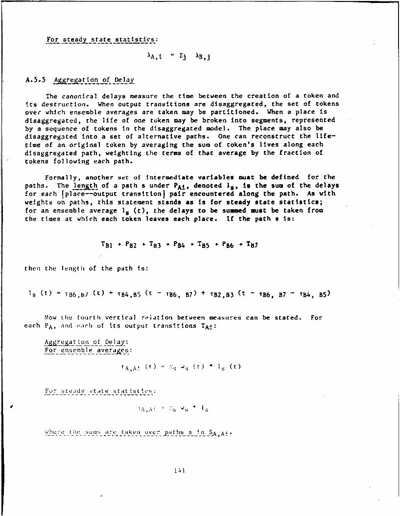
For steady state statistics:
AA,i = -j XB,J
A.5.5 A eration of Delay
The canonical delays measure the time between the creation of a token andits destruction. When output transitions are disaggregated, the set of tokensover which ensemble averages are taken may be partitioned. When a place isdisaggregated, the life of one token may be broken into segments, representedby a sequence of tokens in the disaggregated model. The place may also bedisaggregated into a set of alternative paths. One can reconstruct the life-time of an original token by averaging the sum of token's lives along eachdisaggregated path, weighting the terms of that average by the fraction oftokens following each path.
Formally, another set of Intermediate variables must be defined for thepaths. The len &_h of a path s under PAi, denoted J., is the sum of the delaysfor each 1ploce--output transitioni pair encountered along the path. As withweights on paths, this statement stands as is for steady state statistics;for an ensemble average I (t), the delays to be summed must be taken fromthe times at which each token leaves each place. If the path s is:
TBI ÷ PB2 + TS3 * PB4 * TB 5 * Bb * TB7
then the length of the path is:
IS (t) TB6,h7 (t) + TB4,B5 (t - TB6, B7) + TB2,B3 (t - 116, B7 - TB4, B5)
Now the fourth vertical r,-iation between measures can be stated. Foreach PA, and ,arch of its output transitions TA;:
_A~fr e_.a.t~to2 o_ fDeljay :
For ensemble averages:
t.\A4 (t) A: !.; (t) * 1s (t)
For stead_ st tte _statistcs:
`A,.- = :s '-s * S
Where the sums are taken ovar paths s--
141

A.5.6 1i21ications for MinimaLLty
If the prescription for Fact A-1 to hold is followed, it will be ensu:edthat every transition and place at level N is disaggregated, perhaps trivt-ally, into elements at level N+1. If this Is the case, it has been shown thata vertical relation can be constructed for every level N measure. Thus know-ledge of the values for all level N+1 measures completely determines valuesfot all level N measures. Thus the level N measures are redundant. If oneseeks sets of measures that are independent, then one can only take measuresfrom one level at a time.
Therefore, the ultimate set of measures desired are those from one level
of a hierarchical STAPN model. Since theru is une set for each level of themodel, nested sets of measures have indeed been const'iicted, where higherlevel ,reasures are simple aggregations of lower level measuz-ts.
A.6 EVALUATION OF MEASURES
Now all of the basic concepts re 4 uired to systematically generate sets ofmeasures for Command and Control systems are in place. For completeness, areview of some techniques for computing values for those measure,; is in order.
Although evaluation of measures is outside the scope of this work. numer"uuscomments on evaluation have appeared throughout, and some tt.,chniques terit abrief review.
Evaluation techniques fall into three classes. In increasing order ofexpense, these are ' techniques, where values emerge as the solution toa set of equations; simulation, where the behavior of the system is mimickedby a combination of hardware and software models; and fe_.eri~ments, where thereal system is operated in a manner representative of actual wartime condi-tions. This section cannot review all three techniques in depth, and sofocuses on those aspects which are particularly germane to STAPN models.
The major contribution of the STAPN framework is not a set of new evalua-tion techniques; those listed below are commonly used and well understood.Rather, it establishes a common intellectual framework which facilitates cola-
parisons between data obtained from different evaluations. Thus, for a singlisystem, a numerical analysis, simulation results, and experimental data can bedirectly compared and checked for consIstenCy.
The major question still to be addressed is the construction of enoughadditional relations between measures to permit a single solution f,,r thet!values to emerge. Since the canonical horizontal and vertical relations arisefrom the structure of the network alone, the obvious sources for the addo-tional relations are decision rules, timing models, and attribute maps. Forexample, timing msodels may relate delays to arrival rates and occupancies, anddecision rules may produce models which determine probabilities from delays,occupancies, and rates.
1A2
A.6.1 Analysis
The most highly developed analytic techniques are those from criticalpath analysis and queuing theory. Since both PERT charts and queuing theore-tic models are very similar to STAPN models, although more limited in scope,these techniques can at least be applied to a subset of STAPN models.
Generally, queuing analysis computes steady state values for measures.Additional relations to generate a solution are derived from analyses ofstandard queuing structures, such as single-server, first-in-first-out queueswith reneging from the queue. The equations constructed by these analysesprovide relations between rates, delays, and occupancies, as desired. Unfor-tunately, the equations are strictly correct only when a number of restric-tive, and often unrealistic, assumptions are imposed for the probabilitydistributions of various measures (e.g., the interval between transitionfirings is an exponentially distributed random variable).
Less work has been done on analytic evaluation of ensemble averages.These offer the potential of describing changes in behavior of a system astime progresses, as well as evaluating systems without any well definedsteady state. At best, current technology permits differential equationsto be derived for specific ensemble averages, such as the occupancy of aplace representing a queue, in rather simple systems with many simplifyingassumptions.
A.6.2 Simulation
Simulation is by far the most popular method for evaluating measures.Simulation has a reputation for providing visibility into the relationsbetween reality and the assumptions built into a model intended to mimic thatreality. This reputation is well deserved, except in cases where complexityoverwhelms an analyst and visibility gives way to obscurity.
STAPN models are quite well suited for simulation. Indeed, a number ofsoftware products have appeared, particularly in Europe, which are tailoredto simulation of some form of Petri net. However, none support all featuresnecessary to directly simulate the STAPN models described in subsection 2.2.(Of course, such models can be simulated indirectly by translating them intothe constructs of existing special purpose simulation languages).
The appeal of STAPN simulation lies in the fact that the basic eventsare transition firings, and these take place at discrete points in time. Themarking of a STAPN changes only at a firing, so data structures need to beupdated only at these times;. Thus STAPNs are ideal candidates for discreteevent simulation techniques, where computational load is determined by thenumber of events which occur in a system, not some arbitrarily chosen inte-gration step size.
In addition, the hierarchical structure of the STAPN models describedhere simplifies the collection of output statistics. As each transition at
143

the lowest model level fires, several measures must be adjusted: the rate forthat transition, the occupancies of Its Input and output places, and the prob-abilities and delays for arcs leading from input places to the transition.The vertical relations determine exactly how to propagarp these changes upthe hierarchy of measures, so that measures at all levels of detail can beaccessed while the simulation is in progress.
However, simulations (including STAPNs) can be expensive ,in two ways.First, to construct a large simulation of a real system is a major softwareengineering effort. The availability of general purpose tools to aid thisprocess has alleviated, but not eliminated, the large amount of manpowerrequired to build a realistic simulation in which all assumptions are con-sistent. Modifying large simulations is also notoriously difficult.
The second expense associated with simulation is computer time. WhIleone replication of a simulation may be rather inexpensive, an extremely largenumber of replications are usually needed for statistically significant ensem-ble averages to be computed.
A.6.3 Exercise and Experients
The faost expensive method for evaluating statistics is also thc most
realistic -- run the real system and see how it behaves. The major drawbackto experiments or exercises is the significance of the results, as very fewreplications can be run to give statiEtical significance to onsemble averages.
The -'ajor potential contribution of Lhe STAPN framework to evaluation byexperiment is in the data collection and reduction processes. Prior to anexercise, data collectors must be instructed to observe and report specificevents. The precision of a well built STAPN model can help define exactlywhat constitutes an event -- exactly what object is to cross what boundary asthe event tai.es place. In addition, the vertical relations contribute as muchto data reduction In this context as to simulation.
A.7 OPEN ISSUES
The concepts described in this section are but a start towards a completemethodology for evaluating C3 systems. The three imost prominent desiderataare: (a) more extensive validation that assertionls I to 5 in subsection 3.4are indeed true, (b) the ability to meld behavioral measures with models forstructures which change over time, and (c) development of analytical tools forevaluating transient values of measures (ehsetable averages) without resortingto the expense of simulatlon or exercise.
A.7.1 Validation
The concepts described herein have been applied to a gencr`c eir defense
mission (see Vol. i1). While no evidence was produced contradicting any of
144
I . . ... . . .. . . .. m I i l l I I I I I I

the assertions presented above, one exercise of a method does not constituteproof of the generality of the method. Air defense is a well, studied, highlystructured mission area. Whether or not (apparently) less structured missionssuch as cover and deception can be reduced to STAPN models remains to be seen.
In addition, one drawback of the concepts constucted above was clearlydemonstrated In both the air defense analysis and in another, similar studyof NORAD's Missile Warning Center: complexity dominates any manual effort.While the hierarchical structure of a model helps manage complexity, there isa limit to the number of pages of diagrams which any person can manipulatesimultaneously. Purely manual validations of these concepts are likely to beexpensive and frustrating. Fortunately, the rigorous framework common to theconcepts opens opportunities for partial automation of STAPN modeling andmeasure generation.
A.7.2 Structural Dynamics
Structural measures convey how the interconnections of a system (i.e.,the topology of a STAPN model) change over tiwe due to failures, repairs,enemy action, or reconstitution. Current evaluation technology generallylimits us to evaluation of behavioral measures in the context of one specificstructure. If the structure of a system changes, then we typicallyre-evaluate the behavioral measures, once for each system structure. In caseswhere behavioral measures are In fact evaluated along with structural changes,little work has been done to carefully define the measures -- time averagesmay not make sense because of intervening structural changes, and ensembleaverages may be-questionable because the system structure may change at dif-ferent times in different replications.
Unfortunately, the changes in system structure are often driven by thebehavioral events. If I C3 system permits attackers to penetrate defensesfrequently, then the t .e between structural changes caused by enemy actionswill be short. Integration of (transient) behavioral measures with structuralmeasures would be much more realistic than present techniques.
A.7.3 Continuous Time Models
Finally, the entire process of evaluating C3 systems should be made morecost effective, so that taxpayers' dollars are spent more wisely and so thatmore comprehensive evaluations can take place, resulting in more effectivefielded systems. Since time varying, ensemble averages provide the mostInsight into system behavior, this means that either simulation technologyshould be improved, or that analyical techniques which directly computeensemble averages should be developed.
The latter notion may not be unrealistic in the context of STAPN models.Recall that the horizontal and vertical relations can be written for ensembleaverages as well as for steady state measures. As with steady state queuinganalyses, there are not enough horizontal relations to completely deteiaine
145

values for the measures. However, it may be possible LO augment the canonicalhorizontal relations with other retlioas derived from timing models or deci-
sion rules. Ideally, these additional relations would take the form of delay-differeutial equations, so that they are compatible with the structure o0 thecanonical relations. With certain approximations, it may be possible to reducethe completed set of delay-differential equations to a set of ordinary differ-ential equations, for which numerous solution Lechniques exist.
146

APPENDIX B
ILLUSTRATIONS OF PETRI NET MODELS REPRESENTING HUMAN-MACHINE INTERACTION
B.1 PURE* PETRI NETS
Pure Petri nets have nodes (places, transitions) and arcs that connectthe nodes to form a network. Often the place nodes represent pre-conditionsor post-conditions of some event, and the transition nodes represent theevent. In other models, the places represent processes, and the transitionsmark beginning-of-processing and end-of-processing. Tokens in places in thenetwork indicate that the pre-conditions (or post-conditions) are true, orthat the processing is in progress. Transitions consume tokens from theirinput places and create tokens for their output places; this can indicate foreyample, that pre-conditions no longer hold, or that processing has begun.Places have only one output transition.
Pure Petri nets are used to model systems for which it is necessary torepresent the coordination of resources or processes. For example, considersimple message-handling by an operator as shown in Fig. B-l.
rMESSAGE ARRIVES
* 1MESSAGE IS WAITING
"OPERATOR BEGINS TO PROCESS MESSAGE
IS IDLE OPERATOR IS PROCESSING MESSAGE
_MESSAGE PROCESSING COMPLETE
IMESSAGE IS AWAITING DISPATCH
iMESSAGE IS SENT
i iu re B- I. Simple Message-lkindling by ai Operator
Wi.e., wi-Tiou0t extensions. "Pure Petri nets" refers to C.A. Petri's originaldescription (1962), as opposed to "extended Petri nets," which includemodific•i i ro; to increase the expressive power of the methodology.
147

In the above example, message-processing can begin because a message iswaiting and the operator is idle.
In Fig. B-2, a r :ssage is waiting -- it cannot begin processing becausethe operator is not idle.
r1ESSAGF ARRIVES
* IMESSAGE IS WAITING
OPERATOR OEGINS TO PROCESS MESSAGE
* OPERATOR IS PROCESSINGr-MESSAGE
MlESSAGE PROCESSING COMIPLETE
M1ESSAGE IS AWAITING DISPATCH
MlESSAGE IS SENT a WO
rigure B-2. Message Waiting
In Fig. B-3, two operators are available. Also, the place whuru inessageswait (prior to sending) has room for only three messages.
- -- rMESSAGE ARRIVES
.MESSAGE IS WAITING
OPERATOR BEGINS TO PROCESSMESSAGE
OPERATOR * OPERATOR IS PROCESSING rlE5SArEIS IDLE
-•ESSAGE PROCESSING COMPLETE
rIESSAGE IS * SPACE IS AVAILADL( FOR MESSAGEAWAITING DISPATCH IN OUTPUT flUFFER
MESSAGE 15 SENT
Figure 1B-3. TwG Operators, Output Buffer of Capacity 3
148

Figure B-4 depicts message handling with confirmation required.
MESSAGE ARRIVES
MESSAGE IS WAITING
REOUEST CONFIRMAT ION
CONFIRMATION REO]UEST MESSAGE WAITINGWAITING
OPERATOR 2 OPERATOR I SIS AVAIL ABLE *AVAILABLE TO
TO OBTAIN PROCESS MESSAGECONFIRMATION
CONFIRMATION IS OBTAINED MESSAGE IS PROCESSED
MESSAGE IS READY TO SEND
MESSAGE IS SENT 2-2692
Figure B-4. Message Processing With Confirmation
In the above figure, the message is ready to send when the message isprocessed and confirmation is obtained.
B.2 LIMITATIONS OF PURE PETRI NETS
B.2.1 No Variation of a Token's Path
It is not possible to model a branch in a token's path (because a placemay have only one output transition).
Consider our first example (Fig. B-i): simple message handling. Weknow that messages are sometimes garbled. Suppose (for simplicity) that onemessage in three is garbled and needs to be queued up for reprocessing.Hlow might we model this? Consider Fig. B-5.
149

'II
MESSAGE IS WAITING TO OE
PROCESSED (OR REPROCESSEO)
-75 12
MESSAGE ISSENT BACK MESSAGE IS BEING PROCESSED
TO BEREDONE
t3
MESSAGE 1S READY TO LIE S[Nr
t4 r1ES5AGE IS 5[ET ON
Figure B-5. Me!;sage Reprocessing
A message that is ready to be sent may follow one of two paths: it may
be sent on, or sent back to be redone. In this simple model, every thirdmessage is sent back -- will it work? Only if it is somehow guaranteed thatwhenever t 4 and t 5 are both enabled, L5 will fire first. t4 and t5 are inconflict, since firing t 5 diser.ables 14. The problem of transitions in con-flict will be considered later.
B.2,2 No Explicit Consideration of Timing Fffe':ts
In pure Petri net modeling, processes are considered to take some indeter-
minate amount of time. The issue is not one of using resources efficiently,but preventing situations such as bottlenecks or deadlock. In parallel pro-cessing situations, tokens may pile up, or resources (operators) be idle, ifthe parallel processes take different amounts of time.
Consider the example in Fig. 13-4: ineCsag, processing with confirmation.Suppose it takes 60 seconds to process a message, but two minutes to obtainconfirmation. The model given slit) represents the necessary coordinationcorrectly - a icssage will not be sent on until it has been processed and
confirmed. But if messages arrive at a ratv laster than one every two min-utes, the processed messages will pile up awaiting confirmation. One caneasily prevent this as shown in Fig. B-6.
In Fig. B-6, the place pI on the right prewvnts either task trom begin-ning until a prior message has been procOs.CeId .nd COnIIJ IIMUc. l)W1'Vetr', 110W O01eoperator will ),e idle 50 percent of the time, and me;sages may pile up awalit-i"ng processing. The model may nut give us iaiy indicatiun. ('[The plaie p)1 ismerely redundant.)
i ! I I I I IIU

MESSAGE ARRIVES
• MESSAGE IS WAITING
CONFIRMATION REQUEST WAITING MESSAGE IS WAITING
IIOPERATOR I ISAYAILAKLE TO
OPERATOR 2 PROCESS MESSAGEIS AVAILA8LE
PTO OBTAIN
CONFIRMATION "MESSAGE ANDCo-FICOWI RATAT OON
ARE BEING
CONFIRMATION IS OBTAINED MESSAGEISPROCESSED
MESSAGE IS AWAITING DISPATCH
MESSAGE IS SENT R.2694
Figure B-6. Message Processing With Confirmation
B.3 EXTENSLtONS OF PETRT NETS
B.3.1 Ex cit Consideration of Branching* in the Net
To mode l systems in which a token may travel from a place to one of twoor more Lrasiitions, we allow explicit branches in the links between placesa nd transitions (Fig. 8-7). Transitions may then "share" common input, places:LWu traifItLioi, might be enabled in such a way that firing one disenables theother.
Tranaition6 s;hown in Fig,. B-7(a) are in contention; we necd a decisionrule associated with P1 to decide where the token should go in the event thatboth transittons, are enabled: e.g. , "Every third token to t2" or "Go to t2
if -2 is enablud."
-FeLri -fi -withloout br;anches are cal led Decision-Free.
151

0 2 D I P 2 01 P2 P _
t2 1i t2 ._] tl 2 tlI
(e) (0) (C) R.29S
In (a) the decision rule In (b) and in (c) there is no contention,
associated with pl deter- so the decision 'ule is not used.mines which transitionwill fire.
Figure B-7. Transitions in Contention
Consider the simple message handling examprle (Fig. B-i), but supposethere are two classes of messages: status messages and alarm messages; natur-ally, the operator should attend to alarm messages as they arrive. This ismodeled as in Fig. B-8.
ALARM MESSAGE STATUS MrESSAOEARRIVES ARRIVES
ALARM MESSAGE STATUS MESSAGEWAITING (D 0 WAITING
St2
ALARM MESSAGE STATUS MESSAGEBEING PROCESSED BEING PROCESSED
Figure B-8. Message Handling With Prioriýy
The decision rule is: token go.,s to t1 if both tI and t 2 are eiabled.
152
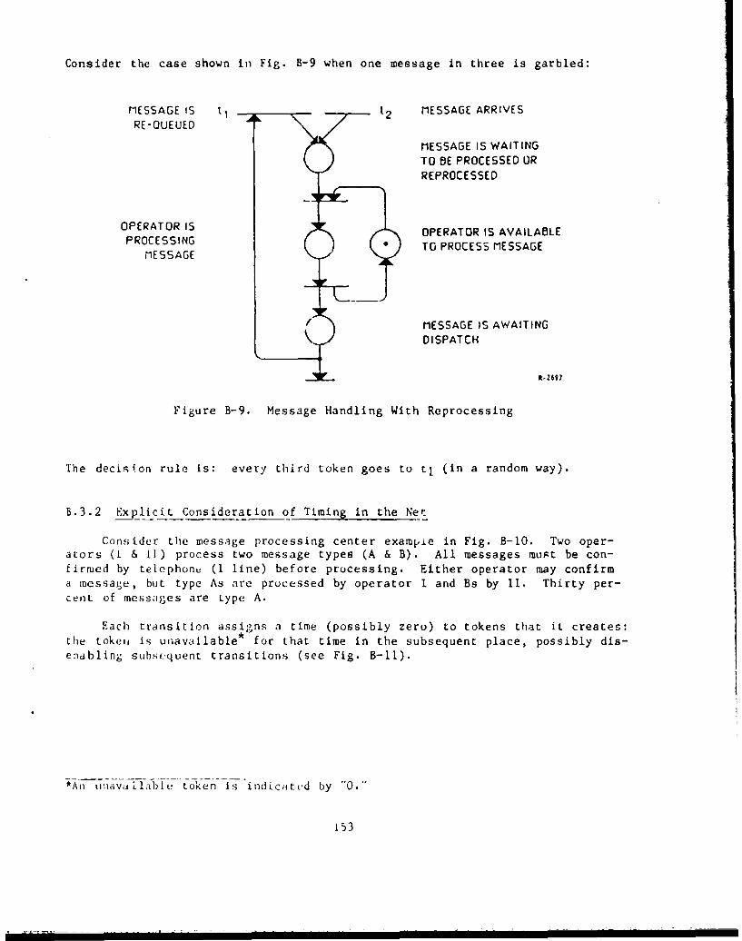
Consider the case shown in Fig. B-9 when one message in three is garbled:
MESSAGERIS ti I. MESSAGE ARRIVES
lMESSAGE IS WAITING
R OTO 6E PROCESSED JRREPROCESSED
OPERATOR IS OPERATOR IS AVAILABLEPROCESSING TO PROCESS MESSAGE
MESSAGE
IMESSAGE IS AWAITINGDISPATCH
SR.z69,
Figure B-9. Message Handling With Reprocessing
The decision rule is: every third token goes to tI (in a random way).
B.3.2 Explicit Consideration of Timing in the Net
Consider the message processing center exampie in Fig. B-1O. Two oper-ators (I & t1) process two message types (A & B). All messages must be con-firmed by telephone (I line) before processing. Either operator may confirma message, but type As are processed by operator I and Bs by II. Thirty per-cent of messages are type A.
Each transition assigns a time (possibly zero) to tokens that it creates:the tokeii is unavailable* for that time in the subsequent place, possibly dis-enabling suhsequent transitions (see Fig. B-li).
*An 1na,1 lal) (I token is indicated by "0.'"
153

18I
2 3
' I 0 mu.26
t1: message arrives PI: message is awaiting confirms-t',: Operator I begins to confirm tion [Rule: output to which-
message ever transition i& enabled,t3t Operator 11 begins to con~firm r 2 if both are enabled]
meestge pz: messeage is being confirmed byt6: Operator I completes confirms- Operator I
tion of message P3: telephone Ia available (Rule:tS: Operator II completea confir- same as I] •
4L
artion ot message Pe: message is being confirmed byt 6 : Operator I begins to procese Operator II
t7: Operator II begins to process P6: message is waiting pzocessingmessage type B [Rule: eend 30 percent of
t8: Operator I completes tokens to t 6 , in a random w.ty]proceessng of meseage type A PY: Operator II Ia idle
t9: Operator II completes P8: message type A being processedprocessing of mese~ge type B by Operator I
t 1 O: message is sent pg: message type B being proce~s,,'by Operator II
PlO; message is waiting to be sent.
Figure B-lO. Message Ptocesslng Center*
W-0i any give-n dyT--fs--likely that the mix of messages (As and bs) wifl only
approximate 30 percent; the actual distribution will vary. The clecis~un rule4 tlc

TOKEN IS PRESENT OUTUNAVAILABLE (FOR TIMEREQUIRED FOR PROCESSING)
t2 t 2 IS NOT ENABLED A-26"
Figure B-11. Unavailable Token
e.g., Consider the message processing with confirmation example (Fig. B-6):processing takes 60 seconds but confirmation takes two minutes (see Fig. B-12):
B.3.3 Considerations of Stochastic Timing
In real life, tasks rarely take precisely 60 seconds, or exactly twominutes. Usually tasks require some time like "two minutes, give or taketen seconds," each repetition requiring a slightly different amount of time.Stochastic-timed Petri nets are as discussed above except tha't the tiresassigned are chosen from an appropriate probablity distribution, so that thetimes given in the example would be "about 60 seconds," "near two minutes"and so forth, depending on the exact times assigned.
B.4 FROMI PETRI NETS TO QUEUING REPRESENTATIONS; STOCHASTIC, TIMED,A ilE:_iT~3 PETRI NETS (STAPNs)
Section 4 of the text discusses queuing theory approaches to IAT. Thefollowing examples Illustrate STAPN representations of simple queuing systems.
B.4.1 Simple G/G/I Queuing Model
ThIc notation X/Y/N is used to describe a queuing system, where X indi-catos zhe nature of the arrival process, Y indicates the nature of the servicet -LStrLbuLion, and N the number of servers.
A G/(;/] queuing system has a general (that is, any) arrival process, ageneral service time distribution and one server: a GIG/I queuing system isany ,iingle server queuing system.
Figure b-13 shouws a block diagram of a single-server queue. Figure B-14shows a I'Qiri net representation of arrivals into the queue, and Fig. B-15shows a Peiri net representation of the queue and service facility. FigureB-16 shows the Petri net rup)esentation of the complete system.
155
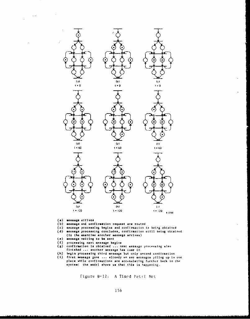
(,0 0(0 0
(d|(W (C)
C.) (hi (ci
t- 0 -0 1.0
0 * 0 0 0
t . 0r i 0 00G
0 0
t -0 1260 1;20
()message arrives(b) message oknd confirmation request are routed(c) teroage processing begins and conf:rmation in being obtained(d) message processing conclude@, confirmation still being obtained
(in the •sentime another message arrives)(e) message waiting to be sent(f) processing next message begins(g) confirmation Is obtained ... next message proce~slng &Ina
finished ... another message has come in(h) bgin processing third message but only second con0irmation(1) first a ssage gone ... already we see messages piling up in one
place while confirmations are accumulating further back In thdsystem: the model shows us that this Is h)ppening.
Figure B-m12 A Timed PeLri Neb
156

ARRIVALS
QUEUEIL 1
1-SERVERFACILITY
DEPARTURES
R-2726A
Figure B-13. Block Diagram of a Single Server Queue
t
R-2727
Figure B-14. Generating Arrivals into the Queuing System
The transition fires whenever the token in the place is available.It consumes this token and creates two output tokens. The tokenthat is output to the place p is unavailable for a time that isdetermined by the inter-arrival distribution. [For example, ifcustomers arrive "every five minutes, give or take a minute or so,"then the time this token is unavailable should be drawn from auniform distribution with mean 5 and standard deviation 1.] Theother token is available immediately.
157

MEANS PI
ANY NUMBER n OFTOKENS naI t
(THE TOKEN IN p3 P3 0 P2
IS UNAVAILABLE)
t 2
R-2728
"a token in Pl indicates "a customer is waiting in the queue"
"a token in P2 indicates "the server is available"
"a token in P3 indicates "the server is attending to a customer"
the firing of tI indicates "service starts for one customer"
the firing of t 2 indicates "service finishes for one customer"
tI fires when tokens are available in Pl and P2" It consumesthese tokens, so there is one less token (maybe none) in p1,and no token in P2- [This corresponds to one less customerin the queue, and the server no longer available.] It createsone token which is unavailable for a time determined by the
service time distribution, and this token goes into place P3,indicating service is in process. [For example, if servicetimes average "three minutes give or take half-a-minute" thenthe time this token is unavailable should be drawn from adistribution with mean 3 and standard deviation .5.]
t 2 fires when the token in P3 becomes available, indicatingservice is ended. It consumes the token in P3 and createsa token for P2 which is immediately available.
Figure B-15. Queuing and Service
IS8

.Pt
tI
P2
t2
P4 *P 3
1-2729
tl: arrival Pl: create arrivalst 2 : begin service P2: queuet 3 : complete service P3: server available
P4: service in progress
Figure B-16. Petri Net Representation of Single Server QueuingSystem at Time T=O.
159

B.4.2 Simple GIG/N Quaeuing Model
"GIG/N" refers to any multi-server queuing model. This model is the sameas the preceding except that P3 contains N tokens (shown as "N-- in Fig. B-17):
*p 1
Ii
122
P4 N e P35
t3
R-.2730
Figure B-17. Petri Net Representation of Multiserver Queuing System at Time T-0
In the f, ilowing (Fig. B-18), a 5-server facility is serving three cus-tomers and no customers are waiting:
*P 1
tP2
P4 oo P3
t3
Figure B-18. Five-Server Queuing Model
160

B.4.3 Simple GIG/N Queuing with Type I Reneging
A queuing system exhibits reneging if a customer leaves the system before
service has been completed. In many situations, a customer will not wait indef-
initely, but will always complete service once service has begun. This customer
leaves the system from the queue only; this is Type I reneging (Fig. B-19).
ARRIVAL
OUEUE
N-SERVERFACILITY
DEPARTURE DEPARTUREAFTER WITHOU'T
SERVICE SERVICE;-??)I
Figure B-19. Block Diagram of Multiserver Queuing System with Type I Reneging
Using Petri Liet notation, we can represent the G/G/N case by adding a
place, a transition and a branch (Fig. B-20):
tI
P3 02
P5 NO P4
514 P
ti : arrival pl: generate arrivals
t 2 : begin service p2: queue available for servie
t 3 : reneg ,i3: queue waiting to reneg
t 4 : end service P4: server available
P5: service in progrejs
Figure B-20. Petri Net Representation of Figure F-19
161
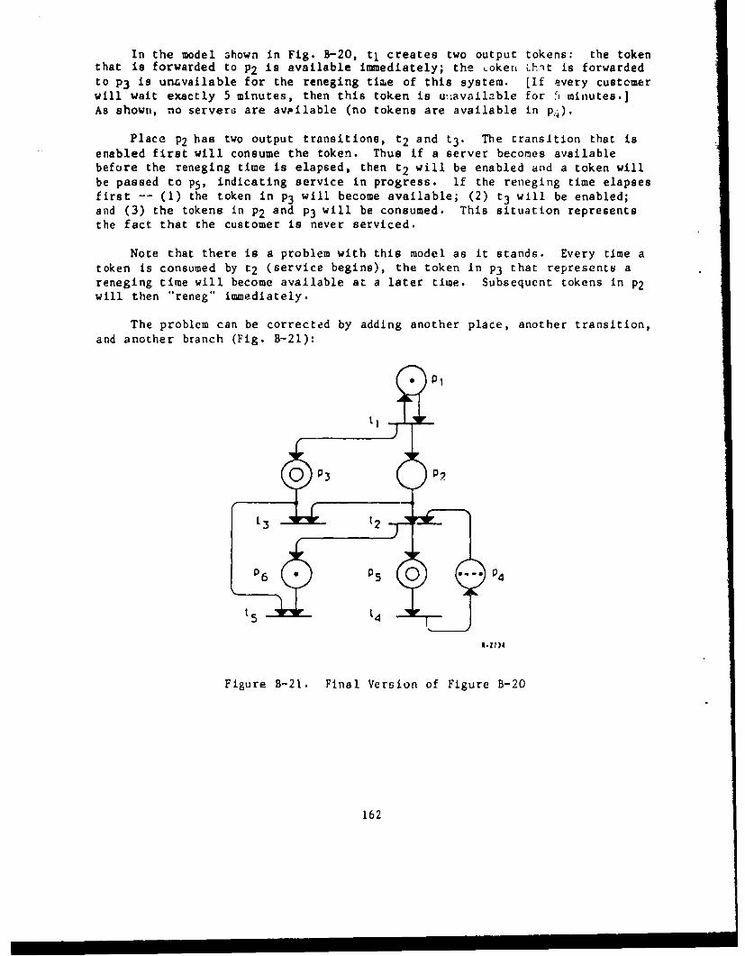
In the model ahown in Fig. B-20, t1 creates two output tokens: the tokenthat is forwarded to P2 is available immediately; the cokert Lhit is forwardedto P3 is unavailable for the reneging time of this system. (If every custcmerwill wait exactly 5 minutes, then this token is w~available for 5, minutes.]As shown, no serverG are available (no tokens are available in P4)"
Place P2 has two output transitions, t 2 and t 3 . The transition that isenabled first will consume the token. Thus if a server becomes availablebefore the reneging time is elapsed, then t 2 will be enabled and a token willbe passed to P5, indicating service in progress. If the reneging time elapsesfirst -- (1) the token in P3 will become available; (2) t 3 will be enabled;and (3) the tokens in P2 and P3 will be consumed. This situation representsthe fact that the customer is never serviced.
Note that there is a problem with this model as it stands. Every time atoken is consumed by t 2 (service begins), the token in P3 that represents areneging time will become available at a later time. Subsequent tokens in P2will then "reneg" immediately.
The problem can be corrected by adding another place, another transition,and another branch (Fig. B-21):
1 )1
It. 2734
Figure B-21. Final Version of Figure B-20
162

Now t2 also creates two output token3 and the token in P6 is available immedi-ately. It represents the fact that processing has started for this customer.When the reneging time is elapsed, the token in P3 becomes available, t 5 isenabled, and the tokens in P3 and P6 are consumed.
A problem still remains. Consider a single server system: one customerbeing served, one customer waiting service, and the reneging time for thefi-7st customer has elapsed (Fig. B-22):
3.13
t 14)
Figure B-22. Contention Between Transitions t 3 and t 5
Now both t 3 and t 5 are enabled. Firing either will disenable the other; thesetransitions are in conflict. We must have a decision rule associated with P3which directs the output of its tokens when both output transitions areenabled. Here we choose a simple deterministic rule: t 5 is always enabled ifthere is a conflict.
Actually, if our implementation allows events to occur "simultaneously,"then we need a decision rule for P2 as well. Suppose in the above example(after firing t5 ) thet the server becomes available (service time in P5elapsed) at precisely the same instant that the token in P3 becomes available(reneging time elapoed). Figure B-23 illustrates this situation:
163

P3 ( P2
to t2 ( o
Figure B-23. Contention Between Transitions t 2 and t 3
Now c2 and t 3 are ii conflict. Here the decision rule we choose for P2 may bedeterministic: "always enter service" (t 2 is enabled) or "always reneg" (t 3is enabled). Or, depending on the situation being modeled, we may feel thatthere is some probability that the customer will reneg, and thus the decisionrule may have probabilistic content: "chances are 60% of customers willreneg;" that is, in a random way, enable t 3 60% of the time.
B.4.4 G/G/N Queuing with Type II Reneging
In some situations, a customer will leave the system after some lengthoZ time (the reneging time) regardless of whether service has begun or not.A system exhibits Type II reneging if customers will reneg fiom the queue orleave while being served. Figure B-24 shows the block diagram to representthis case and Fig. B-25 presents the associated Perr-net model.
ARRIVAL
FACILITY
DEPART RENEGING RENEGINGAFTER FROM FROM
SERVICE SERVICE OUEUE
I-2y],
Figure B-24. Multiserver Queuing System with Type II Reneging
164
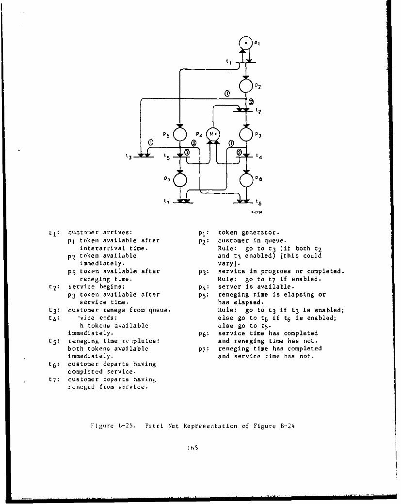
8.211*
•r- t2
P7 P P6
t7 q. t6
ti: customer arrives: pI: token generator.
Pl token available after P2: customer in queue.interarrival time. Rule: go to t 3 (if both t 2
P2 token available and t 3 enabled) [this couldimmediately. vary].
p5 token available after P3: service in progress or completed.reneging time. Rule: go to t 7 if enabled.
t 2 : service begins: P4: server is available.P3 token available after P5: reneging time is elapsing or
service time. has elapsed.
t3: customer renegs from queue. Rule: go to t 3 if t 3 is enabled;t -vice ends: else go to t 6 if t 6 is enabled;
h tokens available else go to t5.immediately. P 6 : service time has completed
t 5 : reneging time ccipletes: and reneging time has not.
both tokens available P7: reneging time has completedimmediately. and service time has not.
t 6 : customer departs having
completed service.t 7 : customer departs having
reneged from service.
Figure 11-25. Petri Net Representation of Figure B-24
165

B.5 EXAMPLE SHOWING USE OF DECISION RULES IN PETRI NET MODELING
A simple model of an operator managing two streams of messages is shown
in Fig. B-26 below:
ENTRY 2 ENTRY 1
0 01
IPILRATOR
SERVICE 2 HFREVO SERVICE 1
EXIT 2 EXIT12.1701
Figure B-26. Model of an Operator Servicing Two Task Streams
If the decision rule at the branch is "allocate the operator (token) to anynonempty queue of messages, this model is complete (tokens flow through thebranch to any enabled transition at the exit of QI and Q2)" If the decisionrule is "allocate the operator (token) to the longest nonempty queue, withties broken in favor of Ql", then thcre if a tradeoff. If this networkdescription is used, then the decision at the branch is =de based un stateinformation beyond 'he enablement status of the transitions terminating thebranch. The number of tokens in QI and Q2 must be compared for the decisionto be made and neither QI nor Q2 is directly connected to the branch. Hencethe simplicity of the network gives rise to a coupling between distant placesand decision rules.
The second decision rule can be implemented by a net where such distantcouplings are absent, albeit at a cost of topological complexity. The deci-sion rule can be decomposed as:
IF 1QIl - IQ21 > 0 THEN serve a token in Ql (P1)
ELSE IF IQ21 - IQII > 0 THEN serve a token in Q2 (P2)
ELSE IF jQIl + 1Q21 > 0 THEN serve a token in QI (P3)
ELSE wait.
166

where IQil is the number of tokens in Q1 at the time an operator token becomesavailable in the "OPERATOR FREE" place. Adding structures to evaluate predi-cates Pl-P3 directly in the Petri net* gives a more complex net, but decisionrules are only dependent upon the enablement status of transitions connectedto the corresponding branch.
In Fig. B-27, IEXCESS Q1 OVER Q21 - IQil - IQ21
JEXCESS Q2 OVER Q11 - IQ2 1 - IQll
ITOTALI = IQWl + IQ21
Tokens become available immediately (after zero delay) in all but the SERVICEiand OPERATOR FREE places.
(NTRY 2 ENTRYI
02 OYER 0 0, OYOER 02
[XFL '2IT T-3T1
Figurc B-27. Adding Structure to Evaluate Decision Rules
-S F B-2e -e f B_--2T.-
167

Decision rules are all of the form "pass the token to the enabld tran-sition with the smallest index"; i.e., the decision rule following OPERATORFREE is:
IF lexcess QI over Q21 >0 THEN FIRE T1
ELSE IF jEXCESS Q2 over Q11 >0 THEN FIRE T2
ELSE IF ITOTALI >0 THEN FIRE T3
ELSE WAIT.
168

APPENDI'" C
PROCEDURES AND GUIDELINES FOR APPLYING IAT TO REAL-WORLD SYSTEMS
C.1 INTRODUCTION
Using modeling notations such as frame/slot and Petri nets to describereal-world systems requires a high-level understanding of system structure,purpose, and re]ationships among elements within a system. The components ofthe IAT conceptual framework have been developed to aid analysts in gainingthis understanding.
Although the focus of work has been to define and refine the modelingtechniques per se, the needs of (prospective) IAT users, who would be requiredto learn the methods themselves and apply them to operational systems, havealso been identified. The subsections below include Aejneric puidqeeiqneýs,intended to support analysts who wish to learn and use IAT techniques for ana-lyzing human/system performance of C3 systems. Examples used in stating theseprocedures have been drawn from ALPHATECII experience to date on modeling theMissile Warning Center (MWC) at NORAD Cheyenne Mountain Complex (NCMC) and ageneric Air Defense System (see Vol. II). The guidelines are presented iierefrom the broadest level of applicability -- model development in general --to a more specific approach geared to analyzing decisionmaking within opera-tional environments such as those found at MWC.
C.2 GENERAL GUIDFLINES FOR IAT MODEL DEVELOPMENT AND USE
1. Define "the Problem:" Why
- Who's asking the question-- Perspective
- When is the answer needed -- Scope
2. Review the Facts: What
- Do not reinvent wheels or probe blind alleys
- Do nut assume non-available Information
169

3. Identify the Analogies: How
- What is this "like" (or not like)
- Where does the analogy begin to fail
4. Develop the Model
- Determine the degree of decomposition needed -- scope
- Identify the variables
5. Formalize the Mathematical (Petri Net) Representation ofthe Model
- Develop the complete model
- Define a complete set of measures
6. Parameterize the Model
- Estimate internal variables (e.g., coefficients basedon resource characteristics and capabilities)
- Estimate external variables (e.g., scenario inputbased on threat and environment characteristics)
7. Solve the Model; Exercise the Representation
- Analytically: Given X, find Y using PERT/CPM or
Queuing Theory Methods
- Numerically: Generate X, compute Y
8. Interpret Results
- Verification
- Validation
9. Sensitivity Analysis
- What is critical/trivial
- 'dow close is good enough
10. Execute Production Runs: Prediction/Estimation
- Interpolate: Precision
- Extrapolate: Speculation
170

C.3 GENERAL RULES TO HELP FOCUS DATA COLLECTION -- FOR BUILDING IATSTRUCTURAL AND PERFORMANCE MODELS
1. For each observed process (activity, task), identify the
following:
a. What constitutes successful completion?[i.e., look for GOALS in the IAT framework]
b. Who normally carries out the process or executes the task?
[identify responsible individuals (RESOURCES),who have specific roles in ORGANIZATIONS]
c. Where is the process carried out?[e.g., workstations, display terminals, other locations(IAT RESOURCES)]
d. How is the process done?
[by what means, using what equipment or information]
c. What triggers the process or permits it to start? to stop?[activation(s), termination(s)]
f. If a process is interrupted, who determines whether toabandon or restart it? What factors influence thatdects~on?
g. After intterruptions, how is restart accomplished?
- with no set-up, some set-up, or complete restart?
- does set-up include activities that would nothave been done otherwise?
h. WhaL happens when performance is blocked?
- required inputs are not available
- required resources are not available
- required authorization is not available
i. Can this process cause other processes to be interrupted?(What happens to resources?)
171

2. Look for inform'ation about each observed process:
a. How often does it occur?[rate or time between events]
b. How long?[speed or duration]
c. How important is it co the purpose of the overall system?[which activities can it pre-empt ... by which otheractivities can it be pre-empted)
d. Where are errors likely to occur?
3. Identify precedence constraints on processes(serial/parallel distinctions):
a. Do things have to happen sequentially? Why?
b. Could things be done concurrently? If so, how couldconcurrent execution be achieved?
4. Describe conditional dependencies (rules and factors):
a. When/if , do , not
b. Unless/until , do
C.4 MORE SPECIFIC GUIDELINES FOR BUILDING IAT STRUCTURAL MODELS*
1. Define the system or subsystem boundary: e.g.,
a. Input bound - message receipt at MWC
b. Output bound - CINC's decision reported outside of NCMC
2. Define the system performance criteria: e.g.,
a. Time that first notification report is transmitted
b. Time that last notification report is transmicted
*Those items marked with "*" will be treated in more detail in subsequent
sections of this appendix.
172

3. Develop a "back-chained logic'* for the data flow sequence:
viz.,
a. Identify content of each output or product (e.g., report).
b. Collect information about how that output is produced,
and by whom* (PROCESSES, RESOURCES, and ORGANIZATIONAL*elements in IAT).
c. Identify each input used in producing each output
(IAT RESOURCES*).
d. Find out how this information relates (i.e., links back)
to the original input bound in the system (e.g., incomingmessage ftream at MWC).
4. Develop a "forward-chained l6gic"* for the data flow sequence:
e.g., for the MWC,
a. Identify all other incoming inpuv messages: their source,content, and arrival characteristics.
b. Identify where and how message existence will first bedetected (with respect to IAT RESOURCES, ORGANIZATIONS,and PROCESSES).
c. Identify each pathway through which message contents mayflow.
d. Trace flows to specific output products or events (eventhough there may be no physical output that is realized;e.g., a file that gets destroyed or a message that raightbe ignored).
5. Identify where in the system human involvement* is requiredto do the following:
a. Decide what option or action alternative to take*, partic-ularly in situations where a decision is on the criticalpath for producing a product or carrying out a task.
,
b. Make a Judgment, without which a data void will exist(or a required output will not be produced).
•-Those hites7 i~a- wi•e -"* will be treated in more detail in subsequentsections of this appendix.
173

C.5 MORE DETAILED PROCEDURES FOR LOWER-LEVEL ANALYSES OF SYSTEM STRUCTURE
C.5.1 Questions to Support Analysis for the 1AT ORGANIZATION Dimension*
I. What is your most important job? [IAT PROCESS]
What is the purpose [IAT GOAL] of this activity?
What do you need to do this job [inputs] and whatproducts or services do you provide [outputs]?
2. If time did not matter, how would you know whether you
succeeded or failed [measure of performance]?
3. Does it matter when the job is done [start, stop,
and/or duration]?
4. Who gets the product [where does it go next]?
5. What makes up the product [what are its component parts]?
6. How is that product built [i.e., put together, assembled,generated or produced]?
7. Where do the inputs come from [ORGANIZATION, other PROCESSES,
and/or other RESOURCES)?
C.5.2 Rules for Hierarchical Decomposition for the IAT ORG.NIZATIONDimension
[Examples based on Missile Warning Center (MWC) and Command Post (CP)at NORAD Cheyenne Mountain Complex (NCMC).J
1. Identify first the single point of authority for the unitbeing decomposed.
- for CP: Command Director
- for rX'C: Missile Warning Officer (MWO)
*Questions at this level of generality should be directed to individuals who
play specific roles in organizations. The question sequence should be re-peated as needed to obtain complete job inventories. Each implied referenceto associated PROCESSES, RESOURCES, and ORGANIZATIONS should be pursued untilelemental tasks can be identified. (An elemental task is a single action ordecision by a human agent, for which a unique output can be identified.)
174

2. Identify subordinate linkages - to whom that individual reportsand who reports to that individual.
- for CINC NORAD: reports to NMCC; Command Director (CD)reports to CINC NORAD
- for MWO: reports to CD; the Events Verification Officer(EVO) and Missile Warning Supervisor (MWS) report tothe MWO.
3. Identify the cooperating and coordinated units.
- Cooperating units supply inputs
- Coordinated units are supplied outputs
4. For each identified organizational element, identify the con-stituent components: the positions that collectively composethis unit.
- for CP, lists of Daily Duty Officers and Battle Staff
- for MWC, list of crew members
5. Prepare an associated Duties List for each individual identi-fied; this serves as a starting point (and later as summarysheet) for the function assignment matrix.
6. If an individual can be at more than one location from time totime, it may become necessary to list these sites. This wouldbe the beginnings of a locatability matrix (especially impor-tant for recall in the transition from peacetime to wartimeoperations).
7. Identify whatever formal documents exist that authorize, govern,or constrain the activities of this organizational unit.
C..; e- 7 I.T RESOURCE Decomposition [based on MWC operations]
I. [See ORGANIZATION decomposition, derived from procedures in sub-section C.5.2, for relevant crew and workstation information.]
2. For each crew position, identify all dedicated console/workstation equipment; all portable/shared equipment; and allpersonnel equipment items.
3. For each equipment item (portable or dedicated), identify allinput/output interfaces and the characteristics of each.
175

4. Within each display identify:
a. what information indicates what is being displayed andhow the operator discerns that,
b. what options can be selected and how these are madeknown to the operator, and
c. the constant and variable contents of each displayformat (for all possible alternate formats).
5. For each control panel, identify the major function being sup-ported and obtain the nomenclature associated with each item(and groups of items) on every panel. Indicate the actuationmode* (push, twist, flip, pull, etc.) for each item.
6. Obtain or document relative position of each item on each panel.and each panel on each console using a well-defined coordinatesystem.
7. Identify or define the operator's work position(s) relative tothe console (standing, sitting, etc.).
C.5.4 Important questions to be Answered About Displays and Controls
1. Display Characteristics of Interest:
a. Are contents always available? Y/N
(If no, name the access procedure)
b. Are changes automatic? Y/N
(If no, name update procedure)
c. Are detections of change highlighted? Y/N
(If yes, by auditory alarm? Y/N)(If alarm no, describe visual display dynamics).
2. Control Characterestics of Interest:
a. Are entries self-paced? Y/N
(If no, what controls the forces pace?)
T-le list should describe what action is required to activate the control;compound actlonu grasp, pull, and lift) may sometimes he required; thesedescriptiotb influence time estimates.
176

b. Are entries fed back for verification? Y/N
c. Are entries checked for validity? Y/N
d. Are transmitted entries acknowledged?
e. Are unacknowledged messages timed out so the operatoris alerted? Y/N
(If yes, how is the alert presented?)
C.6 GENERAL GUIDELINES FOR CARRYING OUT "BACK-" AND "FORWARD-CHAINED"
LOGICAL ANALYSES
C.6.1 Specifying Assumptions:
I. Assume all equipmeit works a:,d crew required is on-handand performing error-free.
2. Anytime there are multiple options:
a. list the entire set
b. determine which dominates (by importance, frequency,or time demanded -- in that order)
c. pursue only the dominant flow path first;pursue others later.
3. Focus on major end products being generated at intermediatestages of evolution toward output; do not explore how these aregenerated (only what, where, when; not how or why).
C.6.2 Guidelines for "Back-Chained" Logical Analysis
PREREQUISITES:
I. Determine the boundary of the facility/organization unit:
Define the I/O interface (what comes in and what goes out).
2. Isolate the I/O component& of interest (e.g., messages).
3. Identify where these manifest themselves inside the unit, i.e.,houndaries where inputs f|nter and where outputs are dispatched.
177

IMPORTANT QUESTIONS:
1. What are the output product(s)?
a. Name the message(s) leaving the facility.
b. Enumerate variable contents of each.
c. Identify the basis for determining which messageleaves in cases where more than one can (e.g., formatselection).
d. For any message, determine what controls its departure.
2. How is each output product composed? [i.e., what are the con-stituents of each output?]
a. For each variable from lb above, identify the exhaustiveset of mutually exclusive alternatives that constitutecontent opinions.
b. Determine who makes the selection; then ask how thatselection is done.
c. For each information item or condition that serveq asan input, identify other items that can be associatedas outputs (within or outside the system boundary).
3. For each identified input, repeat the process described in steps1 and 2.
Quit when all inputs can be viewed as output products fromfacilities which lie outside the boundaries of interest.
C.6.3 Questions for "Forward-Chained" Logical. AnalXsis
1. Identify all input messages, their source and initial destination.
2. Determine buffer characteristics: how many messages can be heldand for how long; when/how might data be lost?
3. What iidicates new/more data are available so that processingmay continue?
4. What are the processing stages between receiving, storing, anddestroying data or information?
178
INE-.

5. How might the information get used (for what, in what, by whom,
and accessed how)?
6. When/how do old files get purged (by whom, on whose authorization)?
7. Can information losses be recovered and if so, how; if not, what
is the impact?
C.7 PROCEDURES FOR ANALYZING HUMAN INVOLVEMENT: SITUATIONS REQUIRINGHUMAN DECISIONMAKING AND JUDGMENT (From Section C.4, No. 5)
C.7.1 Dec1sionmaking
For each decision that is identified:
1. Who normally has decision authority (and under what conditions)?
2. What are the action alternatives from which selection is made?
3. What consequences are of concern?
4. What risks are perceived?
5. What information can change perceptions about the foregoing?
C.7.2 Juagment
For each judgment:
I. Who normally makes the judgment?
2. What changes when the judgment is made?
3. What information does the judge access before implementingthat change?
/4. What would data voids* do to the judgment process?
a. lncreaset error
b. Delay change Implementation
c. Reduce confidence
d other
u. Combinait.Ionb of the above
179//1

180

APPENDIX D
PROCEDURES AND GUIDELINES FOR USING DATA FLOW DIAGRAMS TO DEVELOP IAT DATA
D.I INTRODUCTION
Of the methods reviewed earlier in the IAT development effort (Gruesbecket al., 1984),Structured Analysis (SA) appears to have high utility. SA is amanual, graphical, •ad narrative requirements analysis and design method. Itwas developed during the early 1970's as part of L.L. Constantine's StructuredDesign (SD) methodology, which emphasizes deriving processing requirementsbased on a description of total system data flows and state at any specifictime (DeMarco, 1979; Rowell, 1981).
SA is based on top-down decomposition with simple graphical tools. Itsuse is iitended to improve user/analyst communication and provide accurate andeasily comprehended, structured requirements specifications as input to thedesign stages of the system development life cycle.
A complete SA model consists of the following components:
I. Data Flow Diagrams (DFDs)
2. Data Dictionary
3. Mini-Specs
DFDs, which were used in the SIMCOPE and MWC applications, are network repre-sentations of a system portraying the system's component processes and theirinterfaces (data flows). DFD3 serve to partition the system and may be usedto represent manital as well as automated processes. A Data Dictinnary defineseach of the DFD's interfaces in terms of lower-level data flews and/or moreprimitive data elements-. Mini-Specs describe the lowest-level processes inthe DFDs using tools such as Structured English, Decision Tables, and DecisionTrees (Rowell, 1981).
Note that for IAT applications, based in part on the SIMCOPE andMWC validation studies, we are advocatln& the use of DFDs along withframeslot and Petri net notations. Framme-/slot and Petri net model-ing techniques provide more flexible and comprehensive formats fordecomposiae system constituents Into lower-level processes than dothe (often elaborate) narratives required for Data Dictionary andMini-Specs.
181

D.2 PROCEDURES FOR DERIVING DATA FLOWS USING DEMARCO DFDs
The basic components of DFDs and their application to manned C3 systemshave been presented elscwhere (Kornfeld, 1984; Kornfeld et al., 1905). Thefocus of the discussion here is rather to summarize guidelines for helpinganalysts use DFDs along with other IAT modeling tools. For this purpose, onlya brief listing of DFD components appears below (Fig. D-1), with more emphasison notational conventions.
FILE
COMPONENTS
1. Data flows, represented by labeled arrows. (X.Y,Z)
2. Processes, represented by circles; (P1,P 2 )
3. Files or Data Stores, represented by straight lines; FILE
4. Data Sources or Sinks, represented by boxes.
R-Z3) I
Figure D-1. DeMarco Data Flow Diagram
D.2.1 Data Flow Notational Conventions
Data flows are represented by named arrows or vectors. They act as pipe-lines through which packets of data and information of a known composition canflow.* Conventions for deriving data flows include the following (DeMarco,1979; Rowell, 1981):
I. Name all data flows - when no logical relevant name can be foundfor a data flow, chances are there is some error in the DFD.
*Note that DFDs do not show the system's flow of control. A data flow thatis actually a signal to do something (e.g., a flow named Start-Next-Item)should not be portrayed on the DFDs. Control flows re procedural in natureand should be specified elsewhere (e.g., in Petri nets).
182

2. Choose a name which conveys to the DFD reader what the data isand what is known about it (e.g., Raw-Intelligence-Data 1ecomesSAC-Interest-Data in Fig. D-2, which illustrates data analysisprocesses in IIQSAC).
3. Insure that all data flows have different names to avoid coifu-sion for the DFD reader.
4. Hyphenate multiple word data flows to show that they zepreseita single concept.
INTELLIGE14CE RAWCOLLECTION " INTELLIGENCE SAC-INTEREST
*AGENCY DT NTLAIN
RET RAN SM ISS IDIREQUEST IT
DATA SACINTEREST
IRRELEVANTDAA// DATA
ANALYZEANALYST DATA REJECTED
REPORT FILE ROUTINE ATAINTELLIGENCE RET
PRIORITY DATAINTELLIGENCE•
ROUTINE \REPCRT CURRENT INTELLIGENCEREPOT REORTS DATA BASE
S•./PRIORITYREPORT
lVil;aire 0-2. D~aLi Flow Diagramr of Hlypothetical MilitaryI, t,•lIlgence System (Rowell, 1981; p. 60)
483
--------------------------- P-- -- --

5. When applicable, show data flows diverging to different elementsor converging from different elements with forkiLn or ý_noLvectors, e.g., Relevant-Routine-Reports in Fig. D-2.
6. Let data flows into and out of simple files be identified by thefile name instead of naming the data flow itself (e.g., the dataflow from the SAC-Interest-Installation file to the Edit Dataprocess in Fig. D-2).
D.2.2 Conventions for Other DFD Components: Processes L Files, and DataSources (Rowell.j 1980)
Processes are transformations of one or more incoming data flows intoone or more outgoing data flows (e.g., Edit Data, Analyze Data in Fig. D-2).Processes are represented by circles which are labelled with a number and adescriptive name. The numbering system and its rationale are part of theleveled DFD concept which is explained below.
Files are temporary repositories of data which include a computer tape ordisk, an index file in someone's desk, a computer database, or even a waste-basket. They are represented by a straight line with the file's (descriptive)name in close proximity (e.g., the Analyst Report File in Fig. D-2). Thedirection of data flows going to or from a file is important, showing that afile only provides data to a process (outgoing arrow such as from the SAC-Interest-Installations file to the Edit Data process in Fig. D-2), only re-ceives data from a process (incoming arrow such as from the Write IntelligenceReport process to the Analyst Report file in Fig. D-2), or both. When thereis two-way access between a file and a process, either a double-headed arrowor two separate arrows can be used to show the data flow depending on whetherthe data flows in question have the same composition. The rule is tolonlshow net flows to and from files.
Sources and sinks are net originators or receivers of data which areoutside the system's context and are represented by a named box (e.g., Intel-ligence Collection Agency in Fig. D-2). Data can flow both into and out ofa source/sink box. ThI3_ should be used sparin~gly! since they are usually notdefined very rigorously and are included to provide a feel for the system'sconnections to the outside world.
D.3 RULES FOR DRAWING DFDs (Rowell, 1981; pp. 63-69)
D.3.1 General Guidelines
1. Identify the system's net input and output data flows and drawthem around the ed e of the dia ram. These data flows definethe system's context boundarjy (since everything outside them isout of the system). Try to identify all of the important andrelevant boundary data flows and include them, but do not beoverly concerned with completeness at this point.
184

2. Work from inputs to out -- d. awing in outputs, backwards fromoututsto ro te cetrout' drwif ocesses
and data flows. Concentrate first on major data flows lookingfor primary data pipelines. Draw them on the diagram with (fornow) empty circles for the transforming processes and try tohook them up with the peripheral data flows. Examine each.blank process and see if there are internal data flows whichrequire the process to be split into two or more separate proc-esses. For each data flow item, determine what is needed tobuild it, identify where the components come from, and try todetermine what processes create the components.
3. Carefully label all the interface data flows. The names givento data flows will have a major impact on DFD readability.Therefore, try to make the name appropriate (applicable to theentire data flow, not just one of its components) and avoidgrouping unlike items into a single flow unless they definitelybelong together. Insure all data flows (except to and fromsimple files) are named. If the data flows cannot be simplyand accurately named, consider: (1) breaking them up into twoor more nameable data flows, or (2) restarting.
4. Label the processes in terms of their inputs and outputs. Again,make sure the name is appropriate and reflects what is done inthe transformation. Try to develop names with a single strongaction verb and a single object (multiple verbs usually meanmore partitioning is required). Avoid verbs like "process" or"handle"'- they are too imprecise. Repartition when necessary(to break down processes which are unnameable or to combineseveral processes to describe a process which is more easilynamed).
5. Ignore initialization or termination ideas. Draw the systemin an up-and-running steady state and defer concerns about howthe system got there until later (at the end of the entire DFDanalysis process).
6. lanore the details of trivial error-handlinpdata flows.
If the error requires no undoing of past processing,ignore it for the moment; if it requires you to backout previous updates or revert a file or files to aprevious state, then do not ignore it (DeMarco, 1979;p. 68).
Remember that a DFD is trying to convey an overall picture ofthe system's context and contents -- leave the details untillater.
185

7. Do not portray control flows or control information. Thereare two tests to determine if a data flow is in Fact a controlflow: (1) ask what data or information moves over the dataflow in question -- if there is none, the data flow probablydoes not represent the stream of the data itself and should beremoved; (2) ask what use the destination process will make ofthe data or information moving over the data flow in question.
If it is modified and put out as an outgoing data flowor part of one, then it Is a legitimate data flow. Ifit only serves to prompt the process to start doingits work or guide it in how to do its work, then it iscontrol (DeMarco, 1979; p. 69).
8. Be prepared to start the drawings over. The final DFD set shouldbe preceded by several successively more accurate iterations.
D.3.2 Leveled D'Ds
Leveled DFD• are called for when a system is too large or complex to becompletely represented by a one-page DFD. Leveling involvep first partition-ing a system into subsystems, then treating each subsystem as a system whichis partitioned into sub-subsystems, etc. until the required level of detailcan be achieved for each of the lowest level processes.
The highest-level DFD (i.e., the 6ystem view) is referred to as the"parent," and lower-level DFDs (i.e., subsystem views) are ichildren," in the
DeMarco DFD nomenclature. Insuring the equivalence of data flows betweenparent and child diagrams is called balancing.
D.3.2.1 Notational Conventions for Leveled DFDs
0 Numbering -- Each child diagram retains the number of its par-ent's (related) process circles. Subprocesses are numbered inturn with decimal point separators. For example: Fig. D-3below represents a more detailed (subsystem) view of higher-level processes which were pictured in Fig. D-2. The parent is"Diagram 0" and the child "Diagram I." Process #I, "Edit Data"on Diagram 0, is decomposed into its constituent processes onDiagram 1, the child. Each subprocess on Diagram 1 is labeledas 1.1, 1.2, etc. If a process such as 1.2 were to be brokendown further, the decomposition DFD would be labeled "Uiagram1.2" and the subprocesses 1.2.1, 1.2.2, etc.
186

RAWDATA
VERIFY SAC-INTERESTDATA VERIFIED RAW IhSTALIATIGNS
(Rowel, 198;0. 67) LIGNC
DATA
REI RA4SMI SS IONCOPR
REQUEST DOMATA
UNLISTED
INSTALLAT IONDATA
4 VERIY DATAINSTALLATIO1NIRRELVANCYDATA
hLEVANTUNLISTED
INSTALLATION
I kREL VANITDATAD1T4
DATAR•,OR)AAT SAC
DATA INTERESTj DATA
Figure D-3. Diagram 1: Data Flow Diagram of "Edit Data" Process
(Rowell, 1981; p. 67)
D.3.2.2 Guidelines for Decomposition with Leveled DFDs
I. Asymmetry is allowed when trying to assess which processesshould be decomposed. Some processes are likely to be morecomplex than others -- the more complex processes should bedecomposed down more levels.
2. Stop decomposition when each lowest-leve. process can be speci-
fied by describing elemental tasks and procedures. Using IAT,one should be able to complete a frame by filling in values forslots at the point each lowest-level process has been adequatelydescribed.
3. Maintain accuracy and consistency In carrying out a leveled-DFDanalysis:
"* Show cihanges on both parent and child diagrams.
"* Insiirv that data flows balance.
"* Suspect processes or files with incoming but not outgoingdara flowb; such processes/files may actually be sinks or
187
IV;

p
188

REFERENCES
Bachert, R.F., K.H. Evers, and P.R. Santucci, "SADT/SAINT Simula'ion Technique,"Proc. 1981 National Aerospace and Electronics Conference, Dayton, Ohio, 1981.
Barr, A. and E.A. Feigenbaum, The Handbook of Artificial Intelligence Vol. I,William Kaufman, Los Altos, California, 1981.
Beer, J., Cybernetics and Management, John Wiley and Sons, New York, 1959.
Berne, E., The Structure and Dynamics of Organizations and Groups,J.B. Lipincott, 1963.
Blitz, A.L., J.L. Teele, R.R. Tenney, and L.C. Kramer, "Micro-Modeler User'sManual," TR-273, ALPIATECH, Inc., Burlington, Massachusetts, 1985.
Boehm, B., Software Engineering Economics, Prentice-Hall, Englewood Cliffs,New Jersey, 1981.
Brooks, F.A., Jr., "Operational Sequence Diagrams," I.R.E. Trans. Human Factorsin Electronics, Vol. 1, No. 33, March 1960.
Chubb, G.P., "SAINT, A Digital Simulation Language for the Study of MannedSystems," in J. Moraal, K. - F. Kraiss, (Eds.), Manned System Design: Methods,Equipment, and Applications, Plenum Press, New York, 1981.
Colter, M., R.A. Miller, and J.G. Wohl, "Integrated Analysis Techniques (IAT)for Application to Command, Control, and Communications Systems," TM-HU-566/000/00, System Development Corporation, Huntsville, Alabama, September 1982.
DeMarco, T., Structured Analysis and System Specification, Prentice-Hall,Englewood Cliffs, New Jersey, 1978.
Goode, H.H., and R.E. Machol, System Engineering: An Introduction to theDesign of Large-Scale Systems, McGraw Hill Book Company, Tcc., New York, 1957.
Gruesbeck, M.A., R.A. Miller, J.G. Wohl, D.L. Kleinman, and G.P. Chubb, "AnIntegrated Analysis Technique (IAT) for C3 Operator Performance Evaluation,"TR-175, ALPHATECH, Inc., Burlington, Massachusetts, February 1984.
Klein, G.A., and J. Weitzenfeld, "Improvement of Skills for Solving Ill-DefinedProblems," Educational Psychology, 13, 1978, pp. 31-34.
Kleinrock, R., Queuing Systems Vols. I & II, Wiley, New York, 1976.
189

Kornfeld, J.R., "Specification and Preliminary Validation of LAT Methods:Executive Summary," TR-223, ALPHATECH, Inc., Burlington, Massachusetts,
December 1984.
Kornfeld, J.R., G.P. Chubb, R.A. MillJ-r, and J.G. Wohl, "Specification andPreliminary Validation of IAT Methods: FY84 Annual Report," TR-224,ALPHATECH, Inc., Burlington, Massachusetts, February 1985.
Larkin, J., J. McDermott, D. Simon, and H. Simon, "Models of Competence in
Solving Physics Problems," Cognitive Science, Vol. 4, 1980, pp. 317-345.
Machiavelli, N., The Prince, 1537, Translation by L. Ricci, Mentor Books,1952.
Miller, J.G., Living Systems, McGraw-Hill Book Company, Inc., New York,Chapter 5, 1978.
Minsky, M., 'Mirsky'"s Framc.tcn Theory," in ineoretical issurs in NaturaiLanguage Processing, R.C. Schank and B.L. Nash-Webber (Eds.), MIT Press,Cambridge, Massachusetts, 1975.
Neustadt, R. and E. May, Thinking in Time: The Uses of History for Decision-makers, The Free Press, New York, 1986.
Pattipati, K.R., J.J. Shaw, J.C. Deckert, L.K. Beean, M.G. Alexandridis, andW.E. Lougee, "CONFIDANTE: A Computer-Based Design Aid for the Optimal Syn-thesis, Analysis, and Operation of Maintenance Facilities," Proceedings 1984AUTOTESTCON, Washington, D.C., November 1984, pp. 390-404.
Peterson, J.L., Petri Net Theory and the Modeling of Systems, Prentice-Hlall,Englewood Cliffs, New Jersey, 1981.
Rasmussen, J., and W. Rouse, Human Detection and Diagnosis of System Failures,Plenum Press, New York, 1981.
Rowell, P.V., "Specifying Users' Requirements in the Context of MilitaryIntelligence Related Computer systems," Report No. LSSR 53-81, Master'sThesis, School of Systems and LogIstics, Air Force Institute of Technology,WPAFB, Ohio, September 1981.
SOFTECH, Inc., Structut'pd Analysis and DeslRn Technique, SOFTECH, Inc.,Waltham, Massachusetts, 1978.
SOFTECH, Inc., "Integrated Computer-Aided Manufacturing (ICAM) Architecture,Part II, Vol. IV - Function Modeling (TDEFo)," AFWAI.-TR-4023, Wright-Patterson
AFB, Ohio, June 1981.
Schank, R.C., and R.P. Abelson, Scripts, Plans, Goals, and Understandinj,Erlbaum Associates, Hlillsdale, New Jersey, 1977.
190

Shaw, J.J., and D.P. Bertsekas, "Optimal Scheduling of Large HydrothermalPower Systems," IEEE Trans. on Power Apparatus anai Systems, Vol. PAS-104,
No. 2, February, 1985, pp. 286-294.
Tenney, R.R., "Systematic Evaluation of Command and Control Systems," TR-288,
ALPHATECH, Inc., Burlington, Massachusetts, April 1986.
Warfield, i.N.,"Intent Structures," IEEE Trans. Systems, Man, and Cybernetics,SMC-3, No. 2, March 1973.
Wohl, J.G., D. Gootkind, and H. D'Angelo, "Measures of Merit for 1"ommand andControl," MTR-8217, The MITRE Corporation, Bedford, Massachusett, 1981.
Yager, R.R., "Linguistic Representation of Default Values in Frames," IEEETrans. on Systems, Man, and Cybernetics, Vol. SMC-14, No. 4, July/August 1984.
I "