Heuristic

© Copyright 2012 by N. N. Taleb.

4

4

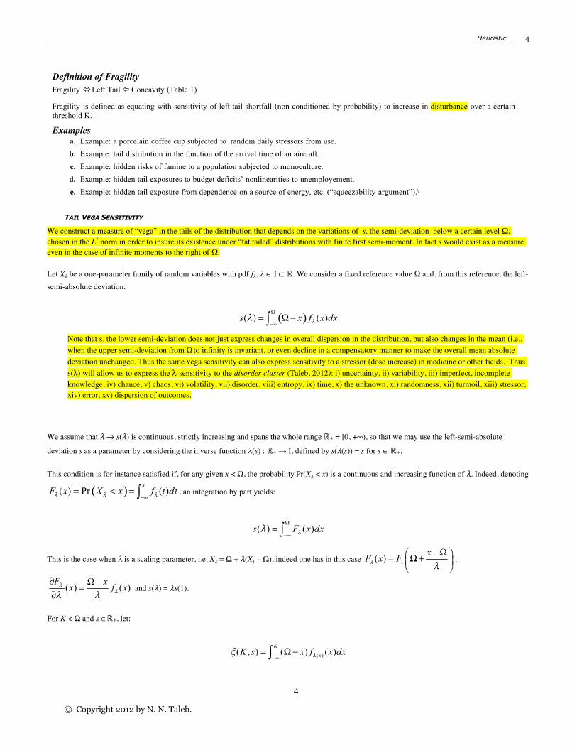
Definition of Fragility Fragility Left Tail Concavity (Table 1)

Fragility is defined as equating with sensitivity of left tail shortfall (non conditioned by probability) to increase in disturbance over a certain threshold K.

Examples a. Example: a porcelain coffee cup subjected to random daily stressors from use. b. Example: tail distribution in the function of the arrival time of an aircraft. c. Example: hidden risks of famine to a population subjected to monoculture. d. Example: hidden tail exposures to budget deficits’ nonlinearities to unemployement. e. Example: hidden tail exposure from dependence on a source of energy, etc. (“squeezability argument”).\

TAIL VEGA SENSITIVITY

We construct a measure of “vega” in the tails of the distribution that depends on the variations of s, the semi-deviation below a certain level Ω, chosen in the L1 norm in order to insure its existence under “fat tailed” distributions with finite first semi-moment. In fact s would exist as a measure even in the case of infinite moments to the right of Ω.

Let Xλ be a one-parameter family of random variables with pdf fλ, λ ∈ I ⊂ ℝ. We consider a fixed reference value Ω and, from this reference, the left-semi-absolute deviation:

Note that s, the lower semi-deviation does not just express changes in overall dispersion in the distribution, but also changes in the mean (i.e., when the upper semi-deviation from Ω to infinity is invariant, or even decline in a compensatory manner to make the overall mean absolute deviation unchanged. Thus the same vega sensitivity can also express sensitivity to a stressor (dose increase) in medicine or other fields. Thus s(λ) will allow us to express the λ-sensitivity to the disorder cluster (Taleb, 2012): i) uncertainty, ii) variability, iii) imperfect, incomplete knowledge, iv) chance, v) chaos, vi) volatility, vii) disorder, viii) entropy, ix) time, x) the unknown, xi) randomness, xii) turmoil, xiii) stressor, xiv) error, xv) dispersion of outcomes.

We assume that λ → s(λ) is continuous, strictly increasing and spans the whole range ℝ+ = [0, +∞), so that we may use the left-semi-absolute

deviation s as a parameter by considering the inverse function λ(s) : ℝ+ → I, defined by s(λ(s)) = s for s ∈ ℝ+.

This condition is for instance satisfied if, for any given x < Ω, the probability Pr(Xλ < x) is a continuous and increasing function of λ. Indeed, denoting

, an integration by part yields:

This is the case when λ is a scaling parameter, i.e. Xλ = Ω + λ(X1 – Ω), indeed one has in this case ,

and s(λ) = λs(1).

For K < Ω and s ∈ℝ+, let:

Heuristic

© Copyright 2012 by N. N. Taleb.

5

5

In particular, ξ(Ω, s) = s. We assume, in a first step, that the function ξ(K,s) is differentiable on (–∞, Ω] × ℝ+. The K-left-tail-vega sensitivity of Xλ at

stress level K < Ω and deviation level s > 0 is:

As the in many practical instances where threshold effects are involved, it may occur that ξ does not depend smoothly on s. We therefore also define a finite difference version of the vega-sensitivity as follows:

Hence omitting the input Δs implicitly assumes that Δs → 0.

Note that ξ(K,s) = –E[Xλ | Xλ < K] Pr(Xλ < K). It can be decomposed into two parts:

Where the first part (Ω – K)Fλ(K) is proportional to the probability of the variable being below the stress level K and the second part Pλ(K) is what, in finance, represents the price of a put option on Xλ with strike K.

Letting λ = λ(s) and integrating by part yields

Where FλK(x) = Fλ(min(x, K)) = min(Fλ(x), Fλ(K)), so that

V ( Xλ , K , s) = ∂ξ∂s

(K , s) =

∂FλK

∂λ(x) dx

−∞

Ω

∫∂Fλ

∂λ(x) dx

−∞

Ω

∫

For finite differences

Where λs+ and λs

– are such that , and .

Heuristic

© Copyright 2012 by N. N. Taleb.

6

6

MATHEMATICAL EXPRESSION OF FRAGILITY

We shall say that a random variable Yµ, depending on parameter µ, is more fragile at the stress level L and semi-deviation level u than the random variable Xλ, depending on parameter λ, at stress level K and semi-deviation level s if the L-left-tailed semi-vega sensitivity of Yµ is higher than the K-left tailed semi-vega sensitivity of Xλ:

V(Yµ, L, u) > V(Xλ, K, s) One may use finite differences to compare the fragility of two random variables: V(Yµ, L, u, Δu) > V(Xλ, K, s, Δs). In this case, finite variations must be comparable in size, namely Δu/u = Δs/s.

A particular case occurs when Yλ = ϕ(Xλ), that is when Xλ is the only driving factor of the risk of Yλ. Let us assume, for the beginning, that ϕ is

differentiable, strictly increasing and scaled so that ϕ(Ω) = Ω. We also assume that, for any given x < Ω, . In this case, as observed

above, λ → s(λ) is also increasing.

Let us denote by gλ the pdf of Yλ and Gλ(y) = Pr(Yλ < y). We have:

Gλ(ϕ(x)) = Pr(Yλ < ϕ(x)) = Pr(Xλ < x) = Fλ(x)

Hence, if ζ(L, u) denotes the equivalent of ξ(K, s) with variable Yµ instead of Xλ, then we have:

Because ϕ is increasing and min(ϕ(x),ϕ(K)) = ϕ(min(x,K)). In particular

Heuristic

© Copyright 2012 by N. N. Taleb.

7

7

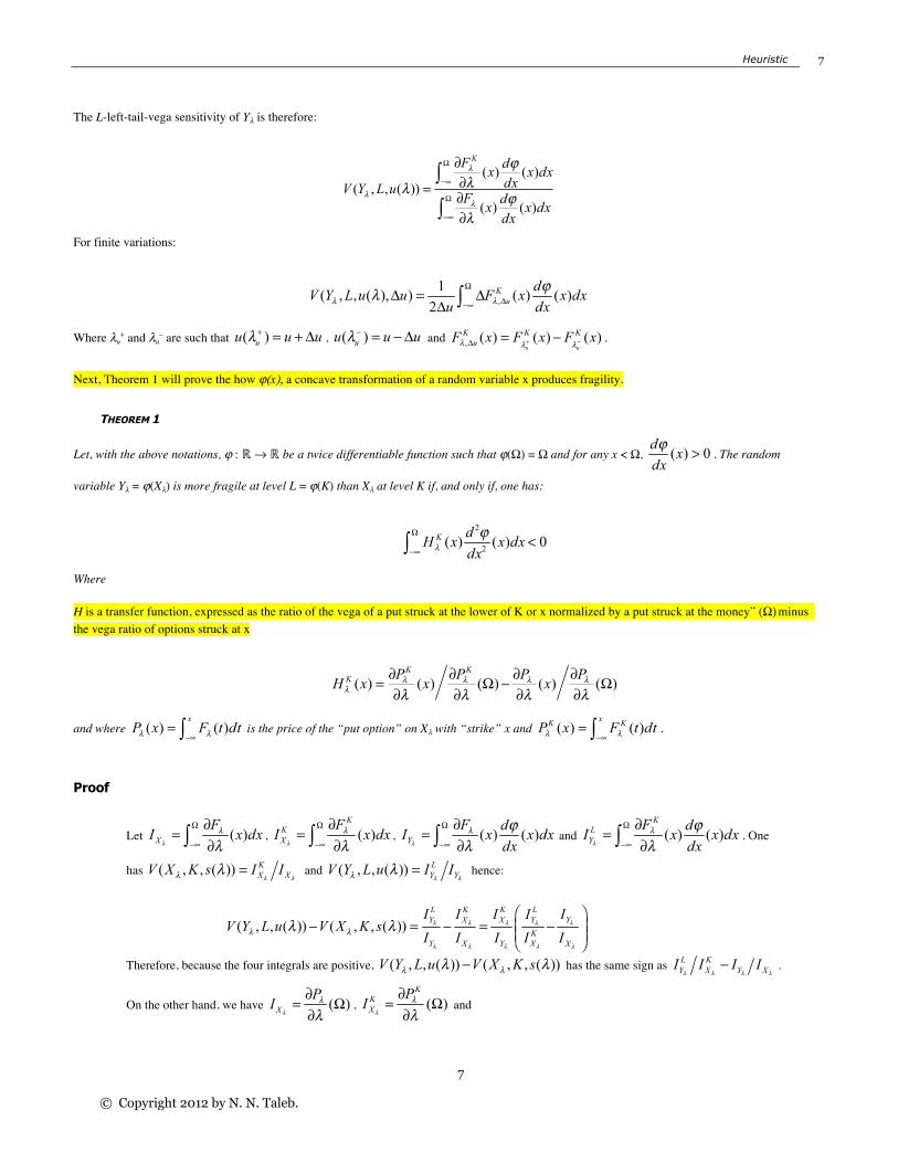
The L-left-tail-vega sensitivity of Yλ is therefore:

For finite variations:

Where λu+ and λu

– are such that , and .

Next, Theorem 1 will prove the how ϕ(x), a concave transformation of a random variable x produces fragility.

THEOREM 1

Let, with the above notations, ϕ : ℝ → ℝ be a twice differentiable function such that ϕ(Ω) = Ω and for any x < Ω, . The random

variable Yλ = ϕ(Xλ) is more fragile at level L = ϕ(K) than Xλ at level K if, and only if, one has:

Where

H is a transfer function, expressed as the ratio of the vega of a put struck at the lower of K or x normalized by a put struck at the money” (Ω) minus the vega ratio of options struck at x

and where is the price of the “put option” on Xλ with “strike” x and .

Proof

Let , , and . One

has and hence:

Therefore, because the four integrals are positive, has the same sign as .

On the other hand, we have , and

Heuristic

© Copyright 2012 by N. N. Taleb.

8

8

An elementary calculation yields:

■

Let us now examine the properties of the function . For x ≤ K, we have (the positivity is a consequence of that of

∂Fλ/∂λ), therefore has the same sign as . As this is a strict inequality, it extends to a an interval on the right hand side

of K, say (–∞, K′ ] with K < K′ < Ω.

But on the other hand:

For K negative enough, is smaller than its average value over the interval [K, Ω], hence .

We have proven the following theorem.

THEOREM 2

With the above notations, there exists a threshold Θλ < Ω such that, if K ≤ Θλ then for x ∈ (–∞, κλ] with K < κλ < Ω. As a consequence,

if the change of variable ϕ is concave on (–∞, κλ] and linear on [κλ, Ω], then Yλ is more fragile at L = ϕ(K) than Xλ at K.

One can prove that, for a monomodal distribution, Θλ < κλ < Ω (see discussion below), so whatever the stress level K below the threshold Θλ, it suffices that the change of variable ϕ be concave on the interval (–∞, Θλ] and linear on [Θλ, Ω] for Yλ to become more fragile at L than Xλ at K. In practice, as long as the change of variable is concave around the stress level K and has limited convexity/concavity away from K, the fragility of Yλ is greater than that of Xλ.

Figure x shows the shape of in the case of a Gaussian distribution where λ is a simple scaling parameter (λ is the standard deviation σ) and

Ω = 0. We represented K = –2λ while in this Gaussian case, Θλ = –1.585λ.

Heuristic

© Copyright 2012 by N. N. Taleb.

9

9

DISCUSSION

Monomodal case

For the earlier theorems to hold, the distribution needs to be monomodal below Ω —otherwise a change in the scale of the distribution might not reflect in “vega” effects.

We say that the family of distributions (fλ ) is left-monomodal if there exists κλ < Ω such that on (–∞, κλ] and on [µλ, Ω]. In this

case is a convex function on the left half-line (–∞, µλ], then concave after the inflexion point µλ. For K ≤ µλ, the function coincides with

on (–∞, K], then is a linear extension, following the tangent to the graph of in K (see graph below). The value of corresponds

to the intersection point of this tangent with the vertical axis. It increases with K, from 0 when K → –∞ to a value above when K = µλ. The

threshold Θλ corresponds to the unique value of K such that . When K < Θλ then and

are functions such that and which are proportional for x ≤ K, the latter being linear on

[K, Ω]. On the other hand, if K < Θλ then and , which implies that for x ≤ K. An

elementary convexity analysis shows that, in this case, the equation has a unique solution κλ with µλ < κλ < Ω. The “transfer”

function is positive for x < κλ, in particular when x ≤ µλ and negative for κλ < x < Ω.

Heuristic

© Copyright 2012 by N. N. Taleb.

10

10

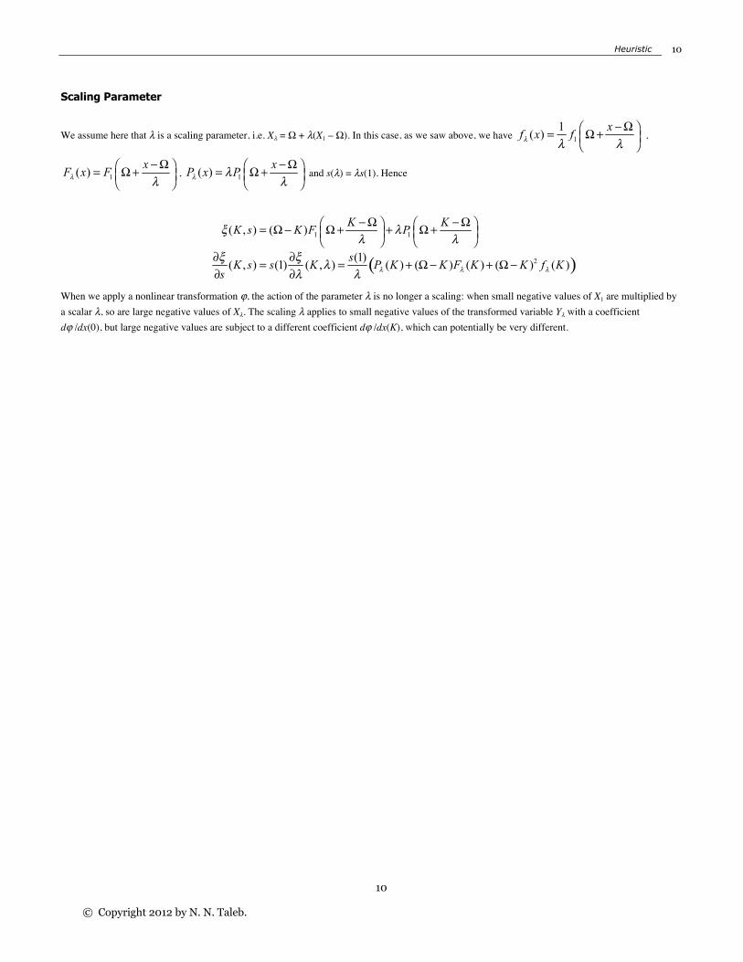
Scaling Parameter

We assume here that λ is a scaling parameter, i.e. Xλ = Ω + λ(X1 – Ω). In this case, as we saw above, we have ,

, and s(λ) = λs(1). Hence

When we apply a nonlinear transformation ϕ, the action of the parameter λ is no longer a scaling: when small negative values of X1 are multiplied by a scalar λ, so are large negative values of Xλ. The scaling λ applies to small negative values of the transformed variable Yλ with a coefficient dϕ /dx(0), but large negative values are subject to a different coefficient dϕ /dx(K), which can potentially be very different.