definition of the iscwsa error model€¦ · errors (such as pipe stand-up) may randomise from...
TRANSCRIPT
Definition of ISCWSA Error Model Rev4 .3 1
Definition
of the
ISCWSA Error Model
Revision 4.3
September 2017

Definition of ISCWSA Error Model Rev4 .3 2
Rev Date By Summary of Changes
4.0 Sep 2016 AEM Initial draft. Numbered to match Rev4 of the MWD model.
4.1 Nov 2016 AEM Corrections to drdpe following spreadsheet development. Addition of flowchart.
4.2 Feb 2017 AEM Incorporate review comments.
4.3 Sep 2017 AEM First release.

Definition of ISCWSA Error Model Rev4 .3 3

Definition of ISCWSA Error Model Rev4 .3 4
1 Scope
This document details the mathematical framework underpinning the ISCWSA error model for
wellbore positioning. The aim is to define the current version of the error model mathematics in one
concise document and as such, it brings together material that was previously available in a number
of SPE papers and ISCWSA documents. This document is intended for implementers and those who
wish to understand the details of the model rather than for users of the model’s results. A
familiarity with the basic concepts of borehole surveying is assumed.
The document is broken down into twelve sections.
Firstly there is an introduction and overview of the constituent elements of the ISCWSA error model
and some comments on what the model does and does not include. Secondly the derivation of the
error model mathematics is described. There then follows some guidance for implementers which
summarises the core model section. Then particular details of the MWD and gyro models are
discussed. Finally, the ISCWSA test wells are specified.
Definition of ISCWSA Error Model Rev4 .3 5
2 Table of Contents
1 Scope ............................................................................................................................................... 4
2 Table of Contents ............................................................................................................................ 5
3 Background ..................................................................................................................................... 7
3.1 Overview of the Error Model .................................................................................................. 9
3.2 Assumptions and Limitations of the Model .......................................................................... 13
4 Details of the Mathematical Framework ...................................................................................... 15
4.1 Definition of Axes .................................................................................................................. 15
4.2 Notation Used in the Mathematical Framework .................................................................. 16
4.3 Notation Used in the Weighting Functions ........................................................................... 17
4.3.1 Note on the use of Azimuth .......................................................................................... 17
4.4 Evaluation of Position Uncertainty ....................................................................................... 19
4.5 Derivation of Weighting Functions ....................................................................................... 23
4.6 Singular Weighting Functions ............................................................................................... 24
4.7 Summation of Uncertainty Terms and Propagation Modes ................................................. 25
4.8 Transformation to Borehole Axes ......................................................................................... 28
4.9 Position Uncertainty Model for a Specific Tool .................................................................... 29
5 Error Sources and Weighting Functions ........................................................................................ 30
5.1 Common Elements of Modelling .......................................................................................... 30
5.1.1 Depth Terms .................................................................................................................. 30
5.1.2 Borehole Misalignments ............................................................................................... 30
6 MWD Modelling ............................................................................................................................ 32
6.1 MWD Revision 4 Position Uncertainty Models ..................................................................... 32
6.2 Weighting Functions ............................................................................................................. 33
6.2.1 Sensor Terms ................................................................................................................. 33
6.2.2 Drillstring Interference .................................................................................................. 33
6.2.3 Geo-magnetic Reference .............................................................................................. 34
6.3 History of the MWD Error Model.......................................................................................... 35
6.3.1 Revision 0 ...................................................................................................................... 35
6.3.2 Revision 1 ...................................................................................................................... 35
6.3.3 Revision 2 ...................................................................................................................... 36
6.3.4 Revision 3 ...................................................................................................................... 36
6.3.5 Revision 4 ...................................................................................................................... 36
Definition of ISCWSA Error Model Rev4 .3 6
6.3.6 Bias Models ................................................................................................................... 37
7 Gyro Models .................................................................................................................................. 38
7.1 Sensor Configuration ............................................................................................................ 39
7.2 Operating Modes .................................................................................................................. 40
8 Utility Models ................................................................................................................................ 43
8.1 Inclination Only Surveys ........................................................................................................ 43
8.2 CNI and CNA .......................................................................................................................... 43
8.3 Testing and Validation .......................................................................................................... 44
9 Implementation ............................................................................................................................ 45
9.1 Inputs .................................................................................................................................... 45
9.2 Output ................................................................................................................................... 45
9.3 Software Flow ....................................................................................................................... 45
9.4 Confidence Level ................................................................................................................... 47
9.5 Example Implementation ...................................................................................................... 47
10 References ................................................................................................................................ 48
11 List of Error Sources and Weighting Functions ......................................................................... 49
11.1 Error Sources Common to Both Gyro and MWD Models ..................................................... 49
11.2 MWD Error Sources .............................................................................................................. 49
11.3 Gyro Error Sources ................................................................................................................ 52
11.4 Utility Sources ....................................................................................................................... 55
11.5 Vertical Singularities ............................................................................................................. 55
11.6 Historic Terms: No Longer Used in the MWD Model After Revisions 3 ............................... 56
Definition of ISCWSA Error Model Rev4 .3 7
3 Background
Like all measurements, borehole surveys are subject to errors and uncertainties which mean that a
downhole survey result is not 100% accurate. For many applications, such as anti-collision and target
sizing, it is very important to be able to quantify the uncertainty in position along a wellbore.
However, since many different factors contribute to the final position uncertainty, determining
these bounds is not a trivial matter.
The Industry Steering Committee for Wellbore Survey Accuracy (ISCWSA) (also known as the SPE
Wellbore Positioning Technical Section) has developed an error model in an attempt to quantify the
accuracy or uncertainty of downhole surveys. This error model consists of a body of mathematics for
evaluating the uncertainty envelope around the survey. The aim is to provide a method of
evaluating well bore position uncertainties based on a standardised and generalised set of
equations, which will cover most scenarios and which can be implemented in a consistent manner in
well planning and directional software.
The model starts from identified physical phenomena which contribute to survey errors, and then
evaluates how these phenomena effect the survey measurements at each station and how these
errors then build up along a survey leg and ultimately along the entire wellbore. Typically the
mathematics are implemented in directional drilling software in which the user selects the
appropriate tool model for use, along with the wellbore surveys or plan in order to obtain an
uncertainty or anti-collision report.
The initial version of the model covered MWD surveys and was described in detail in a SPE paper [1].
This work was later extended with the publication of a gyro model [2] and a depth error paper [3].
There have also been subsequent revisions and corrections of the error models (see section 6.2).
This document sets out to define the current version of the error model. The reader looking for
further details should consult the original papers. Those seeking a more general introduction to the
principles and practises of borehole surveying are referred to the online e-book [9].
Changes to the error model are discussed and agreed via the ISCWSA Error Model Maintenance
Committee. This is an industry wide workgroup and, by prior agreement with the chairman,
attendance is open to anyone who wishes to contribute to the development of the model. See
http://www.iscwsa.net/index.php/workgroups/model-management/ for more details, including
minutes of the latest meetings.
The model may be considered to comprise of two parts; firstly the underlying algorithmic framework
which provides all the mathematical building blocks needed to evaluate and accumulate
uncertainties for any possible tool, and secondly the details required to model a specific tool. These
details are normally defined in what are variously called an Instrument Performance Model, Position
Uncertainty Model, IPM file, tool code or error model. In this document we will use the term
Position Uncertainty Model abbreviated to PUM.
Definition of ISCWSA Error Model Rev4 .3 8
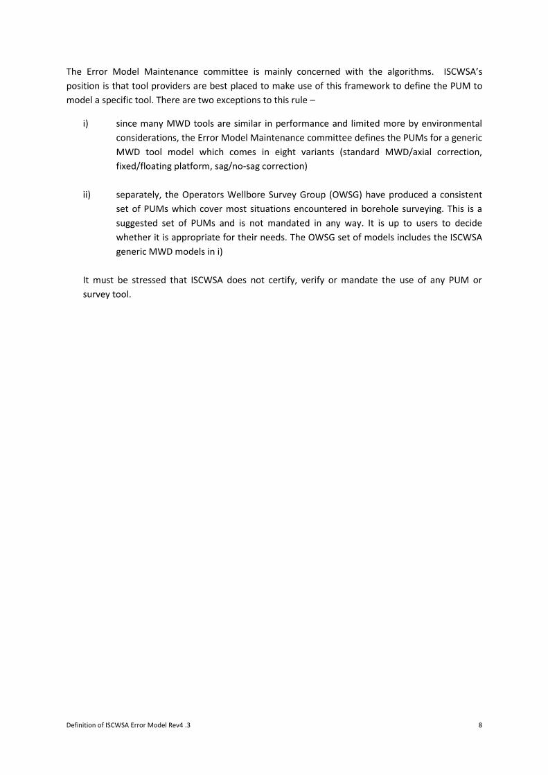
The Error Model Maintenance committee is mainly concerned with the algorithms. ISCWSA’s
position is that tool providers are best placed to make use of this framework to define the PUM to
model a specific tool. There are two exceptions to this rule –
i) since many MWD tools are similar in performance and limited more by environmental
considerations, the Error Model Maintenance committee defines the PUMs for a generic
MWD tool model which comes in eight variants (standard MWD/axial correction,
fixed/floating platform, sag/no-sag correction)
ii) separately, the Operators Wellbore Survey Group (OWSG) have produced a consistent
set of PUMs which cover most situations encountered in borehole surveying. This is a
suggested set of PUMs and is not mandated in any way. It is up to users to decide
whether it is appropriate for their needs. The OWSG set of models includes the ISCWSA
generic MWD models in i)
It must be stressed that ISCWSA does not certify, verify or mandate the use of any PUM or
survey tool.

Definition of ISCWSA Error Model Rev4 .3 9
3.1 Overview of the Error Model
The basic measurements which constitute a borehole survey generally consist of a number of
measured depth, inclination and azimuth values, taken at discrete intervals along the wellpath.
Directional software will use these measurements and assumptions about the shape of the wellpath
between the stations (typically minimum curvature algorithms) to determine the 3D position of the
well as Northings, Easting, TVD co-ordinates.
The purpose of the error model is to evaluate the effects of the various physical factors which lead
to errors in the survey measurements and hence to determine uncertainty in the 3D position.
For a given survey tool, a number of different physical characteristics will be identified which could
lead to errors. The effect of each of these on the measured depth, inclination or azimuth at a
particular survey station is evaluated and in turn the effect on the wellbore position is determined.
The effect of each error is then accumulated along the wellpath and the contribution of all the
individual errors are combined to the give the final uncertainty in wellbore position.
Within the error model, this uncertainty is held as a covariance matrix which describes the
uncertainty along each co-ordinate axis and the correlations between these uncertainties. In
directional software this covariance matrix is commonly used to determine an uncertainty ellipsoid
at a particular confidence level. This ellipsoid may be shown graphically, represented in reports or
projected onto a given plane, in which case it becomes an ellipse and ellipse semi-major, semi-minor
axes can be reported in the plane. The ellipsoids from neighbouring well paths are used in anti-
collision calculations to determine whether drilling a well at that location is allowable or not.
For example, assume that we have a certain survey tool (either a gyro or MWD) which contains
three accelerometers used to determine inclination. We consider that after calibration each sensor
could exhibit a bias (or offset) error, which is a common way to consider sensor errors. From sets of
test data across different tools and runs we determine the typical range of that bias error and
quantify it as a standard deviation.
Then, for a given wellbore survey, we evaluate the effect that an x-axis accelerometer bias error,
with that standard deviation, would have on the inclination and azimuth measurements which we
obtained at each survey station. Note- measured depth in this example comes purely from wireline
or drill-pipe measurements and accelerometer bias errors do not affect the depth readings.
By this procedure, the survey measurement uncertainty (the x-accelerometer bias error) has been
converted into an associated angular uncertainty. From this we can determine the uncertainty in the
3D position of the well at each point along the survey run due to possible x-accelerometer biases.
We can repeat the same process for a y-accelerometer bias, for a z-accelerometer bias and so on for
all the significant sources of error that we can identify for this tool. All of these error values are then
accumulated to determine the position covariance matrix at each station along the well.
Definition of ISCWSA Error Model Rev4 .3 10
It should be noted that we are not evaluating the actual accelerometer bias values during this run.
Instead, we are assessing the uncertainty in well position, due to the likely range of errors that we
can anticipate for these sensors. The output answer is therefore a statistical estimate of the
expected uncertainty for a particular survey.
In the description above, the uncertainties are repeatedly said to be ‘accumulated’ along the well.
That accumulation happens on a statistical basis.
The errors caused by a specific error source (for example, the x-accelerometer bias error) from
survey to survey may be correlated if the underlying sensor error value does not change. Other
errors (such as pipe stand-up) may randomise from survey to survey and are said to be uncorrelated.
Where the errors are correlated (i.e. expected to have the same value from point to point) the
uncertainties are added in the usual arithmetic way. However, if the errors are un-correlated then
we consider that they will be different from point to point and there is chance that different errors
may cancel. In that case, since it is the standard deviation of the errors that we are dealing with, the
uncertainties are root summed squared together.
When combining the contributions due to all of the individual error sources, it is a basic assumption
of the model, that all of the individual error sources are independent (uncorrelated) from each
other. This means that for example the actual x-accelerometer error of one measurement is
independent from the y-accelerometer error at the same (or any other) survey station, as well as
independent from the z-accelerometer error, the depth error, the sag error, etc. This independency
allows for individual conversion into position uncertainties before summation.
Having described the model, we can now identify the various components that are required to run
the calculations:
i) for a particular survey tool we have a number of error sources which effect downhole
surveys. These are identifiable physical phenomena which will lead to an error in the
final wellbore position; for example the residual sensor error after calibration.
ii) each error source has an error magnitude, which is the standard deviation of that error
as determined from test data.
iii) each error source has a set of weighting functions, which are the equations which
describe how the error source effects the survey measurements of measured depth,
inclination and azimuth.
iv) each error source also has a propagation mode which defines how it is correlated from
survey station to survey station, survey leg to leg and well to well, and this is used in
accumulating the errors.
Typically these components are defined within the PUM for a particular tool and
although not strictly necessary within the PUM, each error source generally has an
associated:
v) error code string such as ABZ or MSZ. This is simply a shorthand identifier.
Definition of ISCWSA Error Model Rev4 .3 11
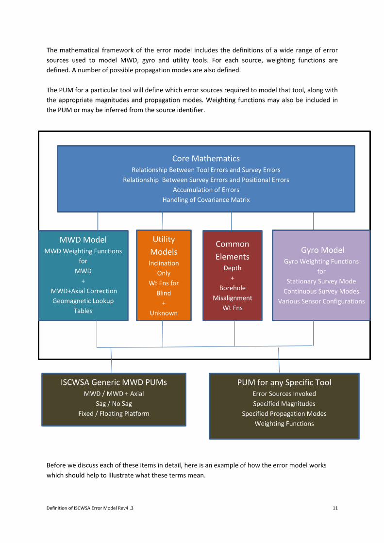
The mathematical framework of the error model includes the definitions of a wide range of error
sources used to model MWD, gyro and utility tools. For each source, weighting functions are
defined. A number of possible propagation modes are also defined.
The PUM for a particular tool will define which error sources required to model that tool, along with
the appropriate magnitudes and propagation modes. Weighting functions may also be included in
the PUM or may be inferred from the source identifier.
Before we discuss each of these items in detail, here is an example of how the error model works
which should help to illustrate what these terms mean.
Core Mathematics Relationship Between Tool Errors and Survey Errors
Relationship Between Survey Errors and Positional Errors
Accumulation of Errors
Handling of Covariance Matrix
MWD Model MWD Weighting Functions
for
MWD
+
MWD+Axial Correction
Geomagnetic Lookup
Tables
Common
Elements Depth
+
Borehole
Misalignment
Wt Fns
Gyro Model Gyro Weighting Functions
for
Stationary Survey Mode
Continuous Survey Modes
Various Sensor Configurations
Utility
Models Inclination
Only
Wt Fns for
Blind
+
Unknown
PUM for any Specific Tool Error Sources Invoked
Specified Magnitudes
Specified Propagation Modes
Weighting Functions
ISCWSA Generic MWD PUMs
MWD / MWD + Axial
Sag / No Sag
Fixed / Floating Platform
Definition of ISCWSA Error Model Rev4 .3 12
Example 1: Declination error
Downhole MWD tools measure magnetic azimuth and in order to calculate the true (or grid) north
azimuth values, the declination term has to be added to the downhole data:
𝐴𝑡 = 𝐴𝑚 + 𝛿 (1)
Usually, declination is determined from a global magnetic model like the BGGM or IGRF models.
However, these work on a macro scale and may not be totally accurate in an oil field. So there is
some uncertainty (or error bounds) on the declination value and this is clearly a possible source of
survey error.
If we include a term dec for these errors then our above equation becomes:
𝐴𝑡 = 𝐴𝑚 + (𝛿 + 휀𝑑𝑒𝑐) (2)
Therefore, the MWD model identifies an error source with the mnemonic code DEC which can be
used to model declination uncertainty. From the above equation we can see that a declination error
will lead directly to an error in the true azimuth, but it has no effect on inclination or depth
measurements.
Hence the DEC weighting functions are [0,0,1] (i.e. md=0, inc=0, az=1). These are about the
simplest weighting functions you can have.
The standard MWD model gives the DEC error source a magnitude of 0.36˚. If an In-Field Reference
survey was carried out in the field then the declination uncertainty would be smaller and there could
be a different tool model (PUM) for MWD+IFR with a smaller magnitude for this error source.
If we assume that, whatever the value, the declination is constant over the whole oil field then all
MWD surveys, with all different survey tools and in all BHA used in all the wells in the field will be
subject to the same error. Hence then DEC term has a global propagation mode.
Declination error is a function of the Earth’s magnetic field and has no influence on gyro survey
tools, so the gyro model doesn’t need to include a declination error term.

Definition of ISCWSA Error Model Rev4 .3 13
3.2 Assumptions and Limitations of the Model
The ISCWSA error model is designed to be a practical method that can be relatively easily
implemented in software and then used by well planners and directional drillers. It is intended to be
applied to a range of tools, used worldwide and accordingly attempts to give good representative
survey uncertainties without the need to model every single variation of tool or running conditions.
The model only applies to surveys run under normal industry best-practise procedures which
include:
i. rigorous and regular tool calibration,
ii. a sufficiently short survey interval to correctly describe the wellbore
iii. field QC checks, such as total magnetic field, gyro drifts , total gravity field and magnetic dip
angle on each survey measurement,
iv. the use of non-magnetic spacing for MWD surveys according to industry norms,
ISCWSA has produced a series of paper which describe the necessary QC process in more detail
[10-11]
It should be recognised that the model cannot cover all eventualities and works on a statistical basis
and so says nothing specific about any individual survey. The results can be interpreted as meaning
that if a well was properly surveyed a number of times by a variety of different tools with the same
specification, then the results would be expected to be randomly distributed with a range of values
corresponding to the error model uncertainty results.
The model cannot cover gross blunder errors such as user error in referencing gyros, defective tools
or finger trouble entering surveys into a database.
The model does not cover all variations and all possibilities in borehole surveying, For example
survey data resolution is not currently modelled.
The model assumes that the wellbore can be adequately described by a constant arc between survey
stations and it aims to evaluate how much errors in these measurements contribute to position
uncertainty. No allowance is made for the survey measurements not being sufficient to define the
wellpath. i.e. the model assumes that IF we could take perfectly accurate inclination, azimuth and
depth measurements we would have an exact value for the wellbore position. As a rule of thumb
this is taken to be a survey interval of 100ft.
Finally, a major misconception is that the ISCWSA provides certified error models for specific survey
tools. The published ISCWSA papers only define the process and equations to work from a set of
error model parameters to an estimate of position uncertainty. The ISCWSA committee does not
define, approve or certify the tool codes containing the actual error model magnitudes which drive
the error model. These should be obtained from the survey contractor who provides the tool, since
they are the ones best placed to understand the specifications and limitations of their tools.
The only exception to this is that there exists a generic ISCWSA MWD model which comes in eight
variants for the combinations of with/without sag correction, with/without axial magnetic correction

Definition of ISCWSA Error Model Rev4 .3 14
and from a fixed or floating platform. The Operators Wellbore Survey Group (OWSG) provide a more
complete set of error models which are available for use.
Definition of ISCWSA Error Model Rev4 .3 15
4 Details of the Mathematical Framework
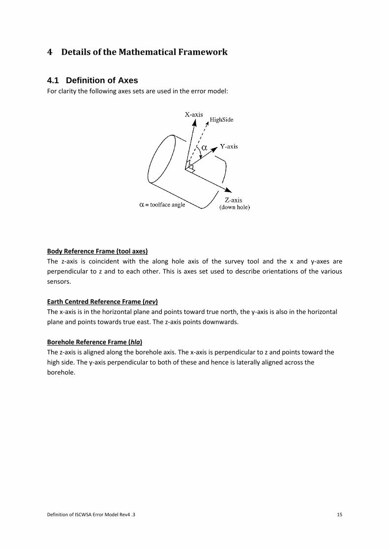
4.1 Definition of Axes
For clarity the following axes sets are used in the error model:
Body Reference Frame (tool axes)
The z-axis is coincident with the along hole axis of the survey tool and the x and y-axes are
perpendicular to z and to each other. This is axes set used to describe orientations of the various
sensors.
Earth Centred Reference Frame (nev)
The x-axis is in the horizontal plane and points toward true north, the y-axis is also in the horizontal
plane and points towards true east. The z-axis points downwards.
Borehole Reference Frame (hla)
The z-axis is aligned along the borehole axis. The x-axis is perpendicular to z and points toward the
high side. The y-axis perpendicular to both of these and hence is laterally aligned across the
borehole.
Definition of ISCWSA Error Model Rev4 .3 16
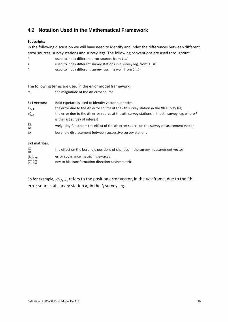
4.2 Notation Used in the Mathematical Framework
Subscripts:
In the following discussion we will have need to identify and index the differences between different
error sources, survey stations and survey legs. The following conventions are used throughout:
i used to index different error sources from 1…I
k used to index different survey stations in a survey leg, from 1…K
l used to index different survey legs in a well, from 1…L
The following terms are used in the error model framework:
𝜎𝑖 the magnitude of the ith error source
3x1 vectors: Bold typeface is used to identify vector quantities.
𝒆𝒊,𝒍,𝒌 the error due to the ith error source at the kth survey station in the lth survey leg
𝒆𝒊,𝒍,𝒌∗ the error due to the ith error source at the kth survey stations in the lth survey leg, where k
is the last survey of interest 𝝏𝒑
𝝏𝜺𝒊 weighting function – the effect of the ith error source on the survey measurement vector
Δr borehole displacement between successive survey stations
3x3 matrices: 𝑑𝒓
𝑑𝒑 the effect on the borehole positions of changes in the survey measurement vector
[𝐶]𝑛𝑒𝑣 error covariance matrix in nev-axes
[𝑇]ℎ𝑙𝑎𝑛𝑒𝑣 nev to hla transformation direction cosine matrix
So for example, 𝒆𝑖,𝑙1,𝑘1 refers to the position error vector, in the nev frame, due to the ith
error source, at survey station k1 in the l1 survey leg.
Definition of ISCWSA Error Model Rev4 .3 17
4.3 Notation Used in the Weighting Functions
The following variables are used in the weighting functions:
Am magnetic azimuth
At true azimuth
B magnetic total field
BH horizontal component of magnetic field
Bx, By, Bz Sensor magnetometer readings in the x,y,z tool axes
c Running speed
D along-hole depth
ΔD difference along-hole depth between survey stations
G Earth’s gravity
Gx, Gy, Gz Sensor accelerometer readings in the x,y,z tool axes
h value of weighting function (used in recursive equations)
I inclination
α toolface angle
Earth’s rotation rate
latitude
Θ magnetic dip angle
γ xy-accelerometer cant angle
f noise reduction factor for initialisation of continuous surveys
k logical operator for accelerometer switching
vd gyro drift
vrw gyro random walk
w12 misalignment weighting term
w34 misalignment weighting term
4.3.1 Note on the use of Azimuth
In borehole surveying we typically make use of three north references – true north, grid north and magnetic
north and therefore we have to deal with three different definitions of azimuth. Care must be taken when
evaluating the error model to use the correct azimuth in the correct place.
Magnetic azimuth, Am, is used throughout the MWD weighting functions (section 11.2), since by their nature
MWD tools measure from magnetic north.
Similarly true azimuth, At, is used throughout the gyro weighting functions (section 11.3) since by their nature,
gyro tools measure from true north.
As defined above, throughout this document the nev-axes north axis is aligned with true north and hence true
azimuth is used in the partial derivatives of the well position with respect to survey measurements (equation 8
– 12) and for creating the direction cosine matrix to transform between the nev and hla axes (equation 30).
Some implementations use a nev-set aligned with grid north. These results can be obtained either by a
rotation by the convergence angle or by using grid azimuth in the appropriate equations.

Definition of ISCWSA Error Model Rev4 .3 18
Even the main published error model SPE papers [1,2] differ in this regard since the MWD paper assumes true
north and the gyro paper assumes grid north. This causes great confusion when comparing results. The
validation dataset sets at www.copsegrove.com are all detailed assuming nev aligned with true north.
Definition of ISCWSA Error Model Rev4 .3 19
4.4 Evaluation of Position Uncertainty
Once we have identified the error sources that will affect our surveys and specified the range of values these error sources may take, we need a means of using that information to determine position error ellipses.
The survey measurements that are taken downhole are the inclination of the wellbore, the azimuth
of the wellbore and the along-hole, measured depth at discrete points. From that information 3-d
wellbore positions are calculated in the appropriate co-ordinate frame by making assumptions about
the path of the well between these survey stations. This is most often done with minimum curvature
algorithms, although other options such as balanced tangential are possible.
The propagation mathematics follows this trail from error source to survey measurements to
position co-ordinates to determine the effect of each error source on the position uncertainty.
The core equation of the error evaluation is:
𝒆𝑖 = 𝜎𝑖
𝑑𝒓
𝑑𝒑
𝜕𝒑
𝜕휀𝑖 (3)
This is a simple chain rule application. We can break this equation down to examine the various
constituent parts.
Firstly
represents the error source (e.g. magnetometer calibration error could be an error source i )
i is used to index which particular error source we are considering
𝜎𝑖 is the magnitude of the uncertainty for the ith error source (i.e. a scalar value, e.g. 70nT)
𝜕𝒑
𝜕𝜀𝑖 are the weighting functions for this source.
These are the partial derivatives of the survey measurements (depth, inclination and azimuth) with
respect to that error source. 𝜕𝒑
𝜕𝜀𝑖 is a 3x1 vector with one term for each measurement, i.e.
𝜕𝒑
𝜕휀𝑖= [
𝜕𝐷
𝜕휀𝑖,𝜕𝐼
𝜕휀𝑖,𝜕𝐴
𝜕휀𝑖] (4)
Hence 𝜎𝑖𝜕𝒑
𝜕𝜀𝑖 is size of the effect of the ith error source on the survey measurements at that point.
ei is the size of the position uncertainty error in nev-axes due to error source i at the current survey
station (a 3x1 vector)
𝑑𝒓
𝑑𝑝 is the effect of the survey errors in md, inc and az on the wellbore position in the NEV axis, (i.e. a
3x3 matrix
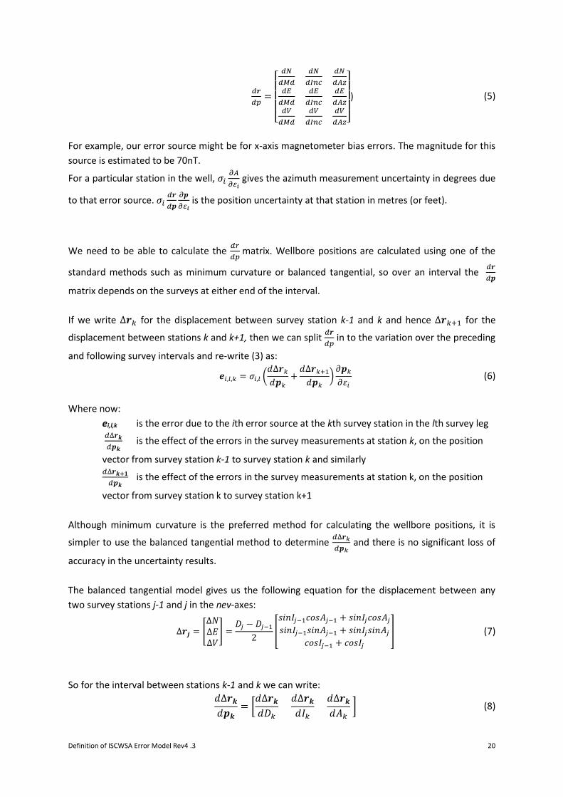
Definition of ISCWSA Error Model Rev4 .3 20
𝑑𝒓
𝑑𝑝=
[
𝑑𝑁
𝑑𝑀𝑑
𝑑𝑁
𝑑𝐼𝑛𝑐
𝑑𝑁
𝑑𝐴𝑧𝑑𝐸
𝑑𝑀𝑑
𝑑𝐸
𝑑𝐼𝑛𝑐
𝑑𝐸
𝑑𝐴𝑧𝑑𝑉
𝑑𝑀𝑑
𝑑𝑉
𝑑𝐼𝑛𝑐
𝑑𝑉
𝑑𝐴𝑧]
) (5)
For example, our error source might be for x-axis magnetometer bias errors. The magnitude for this
source is estimated to be 70nT.
For a particular station in the well, 𝜎𝑖𝜕𝐴
𝜕𝜀𝑖 gives the azimuth measurement uncertainty in degrees due
to that error source. 𝜎𝑖𝑑𝒓
𝑑𝒑
𝜕𝒑
𝜕𝜀𝑖 is the position uncertainty at that station in metres (or feet).
We need to be able to calculate the 𝑑𝑟
𝑑𝑝 matrix. Wellbore positions are calculated using one of the
standard methods such as minimum curvature or balanced tangential, so over an interval the 𝑑𝒓
𝑑𝒑
matrix depends on the surveys at either end of the interval.
If we write ∆𝒓𝑘 for the displacement between survey station k-1 and k and hence ∆𝒓𝑘+1 for the
displacement between stations k and k+1, then we can split 𝑑𝒓
𝑑𝑝 in to the variation over the preceding
and following survey intervals and re-write (3) as:
𝒆𝑖,𝑙,𝑘 = 𝜎𝑖,𝑙 (
𝑑∆𝒓𝑘
𝑑𝒑𝑘
+𝑑∆𝒓𝑘+1
𝑑𝒑𝑘
)𝜕𝒑𝑘
𝜕휀𝑖
(6)
Where now:
ei,l,k is the error due to the ith error source at the kth survey station in the lth survey leg
𝑑∆𝒓𝒌
𝑑𝒑𝒌 is the effect of the errors in the survey measurements at station k, on the position
vector from survey station k-1 to survey station k and similarly 𝑑∆𝒓𝒌+𝟏
𝑑𝒑𝒌 is the effect of the errors in the survey measurements at station k, on the position
vector from survey station k to survey station k+1
Although minimum curvature is the preferred method for calculating the wellbore positions, it is
simpler to use the balanced tangential method to determine 𝑑∆𝒓𝑘
𝑑𝒑𝑘 and there is no significant loss of
accuracy in the uncertainty results.
The balanced tangential model gives us the following equation for the displacement between any
two survey stations j-1 and j in the nev-axes:
∆𝒓𝒋 = [
∆𝑁∆𝐸∆𝑉
] =𝐷𝑗 − 𝐷𝑗−1
2[
𝑠𝑖𝑛𝐼𝑗−1𝑐𝑜𝑠𝐴𝑗−1 + 𝑠𝑖𝑛𝐼𝑗𝑐𝑜𝑠𝐴𝑗
𝑠𝑖𝑛𝐼𝑗−1𝑠𝑖𝑛𝐴𝑗−1 + 𝑠𝑖𝑛𝐼𝑗𝑠𝑖𝑛𝐴𝑗
𝑐𝑜𝑠𝐼𝑗−1 + 𝑐𝑜𝑠𝐼𝑗
] (7)
So for the interval between stations k-1 and k we can write:
𝑑∆𝒓𝒌
𝑑𝒑𝒌= [
𝑑∆𝒓𝒌
𝑑𝐷𝑘
𝑑∆𝒓𝒌
𝑑𝐼𝑘
𝑑∆𝒓𝒌
𝑑𝐴𝑘 ] (8)
Definition of ISCWSA Error Model Rev4 .3 21
Substituting j=k and differentiating equation (7) we get:
𝑑∆𝒓𝒌
𝑑𝐷𝑘
=1
2[
𝑠𝑖𝑛𝐼𝑘−1𝑐𝑜𝑠𝐴𝑘−1 + 𝑠𝑖𝑛𝐼𝑘𝑐𝑜𝑠𝐴𝑘
𝑠𝑖𝑛𝐼𝑘−1𝑠𝑖𝑛𝐴𝑘−1 + 𝑠𝑖𝑛𝐼𝑘𝑠𝑖𝑛𝐴𝑘
𝑐𝑜𝑠𝐼𝑘−1 + 𝑐𝑜𝑠𝐼𝑘
]
𝑑∆𝒓𝒌
𝑑𝐼𝑘=
1
2[
(𝐷𝑘 − 𝐷𝑘−1)𝑐𝑜𝑠𝐼𝑘𝑐𝑜𝑠𝐴𝑘
(𝐷𝑘 − 𝐷𝑘−1)𝑐𝑜𝑠𝐼𝑘𝑠𝑖𝑛𝐴𝑘
−(𝐷𝑘 − 𝐷𝑘−1)𝑠𝑖𝑛𝐼𝑘
]
𝑑∆𝒓𝒌
𝑑𝐴𝑘
=1
2[−(𝐷𝑘 − 𝐷𝑘−1)𝑠𝑖𝑛𝐼𝑘𝑠𝑖𝑛𝐴𝑘
(𝐷𝑘 − 𝐷𝑘−1)𝑠𝑖𝑛𝐼𝑘𝑐𝑜𝑠𝐴𝑘
0
]
(9)
Putting these together:
𝑑∆𝒓𝒌
𝑑𝒑𝒌
= 1
2[
𝑠𝑖𝑛𝐼𝑘−1𝑐𝑜𝑠𝐴𝑘−1 + 𝑠𝑖𝑛𝐼𝑘𝑐𝑜𝑠𝐴𝑘
𝑠𝑖𝑛𝐼𝑘−1𝑠𝑖𝑛𝐴𝑘−1 + 𝑠𝑖𝑛𝐼𝑘𝑠𝑖𝑛𝐴𝑘
𝑐𝑜𝑠𝐼𝑘−1 + 𝑐𝑜𝑠𝐼𝑘
(𝐷𝑘 − 𝐷𝑘−1)𝑐𝑜𝑠𝐼𝑘𝑐𝑜𝑠𝐴𝑘
(𝐷𝑘 − 𝐷𝑘−1)𝑐𝑜𝑠𝐼𝑘𝑠𝑖𝑛𝐴𝑘
−(𝐷𝑘 − 𝐷𝑘−1)𝑠𝑖𝑛𝐼𝑘
−(𝐷𝑘 − 𝐷𝑘−1)𝑠𝑖𝑛𝐼𝑘𝑠𝑖𝑛𝐴𝑘
(𝐷𝑘 − 𝐷𝑘−1)𝑠𝑖𝑛𝐼𝑘𝑐𝑜𝑠𝐴𝑘
0
]
(10)
Similarly, for the interval between stations k and k+1 we can write:
𝑑∆𝒓𝒌+𝟏
𝑑𝒑𝒌= [
𝑑∆𝒓𝒌+𝟏
𝑑𝐷𝑘
𝑑∆𝒓𝒌+𝟏
𝑑𝐼𝑘
𝑑∆𝒓𝒌+𝟏
𝑑𝐴𝑘 ] (11)
Substituting j=k+1 and again differentiating equation (7) we get:
𝑑∆𝒓𝒌+𝟏
𝑑𝐷𝑘
=1
2[
−𝑠𝑖𝑛𝐼𝑘𝑐𝑜𝑠𝐴𝑘 − 𝑠𝑖𝑛𝐼𝑘+1𝑐𝑜𝑠𝐴𝑘+1
−𝑠𝑖𝑛𝐼𝑘𝑠𝑖𝑛𝐴𝑘 − 𝑠𝑖𝑛𝐼𝑘+1𝑠𝑖𝑛𝐴𝑘+1
−𝑐𝑜𝑠𝐼𝑘 − 𝑐𝑜𝑠𝐼𝑘+1
]
𝑑∆𝒓𝒌+𝟏
𝑑𝐼𝑘=
1
2[
(𝐷𝑘+1 − 𝐷𝑘)𝑐𝑜𝑠𝐼𝑘𝑐𝑜𝑠𝐴𝑘
(𝐷𝑘+1 − 𝐷𝑘)𝑐𝑜𝑠𝐼𝑘𝑠𝑖𝑛𝐴𝑘
−(𝐷𝑘+1 − 𝐷𝑘)𝑠𝑖𝑛𝐼𝑘
]
𝑑∆𝒓𝒌+𝟏
𝑑𝐴𝑘
=1
2[−(𝐷𝑘+1 − 𝐷𝑘)𝑠𝑖𝑛𝐼𝑘𝑠𝑖𝑛𝐴𝑘
(𝐷𝑘+1 − 𝐷𝑘)𝑠𝑖𝑛𝐼𝑘𝑐𝑜𝑠𝐴𝑘
0
]
(12)
And so
𝑑∆𝒓𝒌+𝟏
𝑑𝒑𝒌=
1
2[
−𝑠𝑖𝑛𝐼𝑘𝑐𝑜𝑠𝐴𝑘 − 𝑠𝑖𝑛𝐼𝑘+1𝑐𝑜𝑠𝐴𝑘+1
−𝑠𝑖𝑛𝐼𝑘𝑠𝑖𝑛𝐴𝑘 − 𝑠𝑖𝑛𝐼𝑘+1𝑠𝑖𝑛𝐴𝑘+1
−𝑐𝑜𝑠𝐼𝑘 − 𝑐𝑜𝑠𝐼𝑘+1
(𝐷𝑘+1 − 𝐷𝑘)𝑐𝑜𝑠𝐼𝑘𝑐𝑜𝑠𝐴𝑘
(𝐷𝑘+1 − 𝐷𝑘)𝑐𝑜𝑠𝐼𝑘𝑠𝑖𝑛𝐴𝑘
−(𝐷𝑘+1 − 𝐷𝑘)𝑠𝑖𝑛𝐼𝑘
−(𝐷𝑘+1 − 𝐷𝑘)𝑠𝑖𝑛𝐼𝑘𝑠𝑖𝑛𝐴𝑘
(𝐷𝑘+1 − 𝐷𝑘)𝑠𝑖𝑛𝐼𝑘𝑐𝑜𝑠𝐴𝑘
0
]
(13)
In summary, we have now calculated the 3x3 matrix equations which describe the uncertainty in the
wellbore position, caused by errors in the survey measurement at any preceding given station, k.
The 3x3 matrices are evaluated in the nev co-ordinate frame.
Since the wellpaths are built up as a number of curved sections, each of which depends on the
attitude at either end, along most of the wellpath each survey measurement affects both the
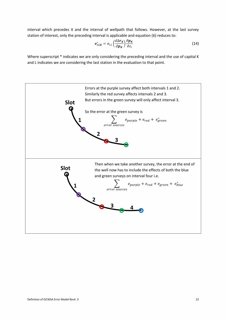
Definition of ISCWSA Error Model Rev4 .3 22
interval which precedes it and the interval of wellpath that follows. However, at the last survey
station of interest, only the preceding interval is applicable and equation (6) reduces to:
𝒆𝒊,𝒍,𝑲
∗ = 𝜎𝑖,𝐿 (𝑑∆𝒓𝑲
𝑑𝒑𝑲
)𝜕𝒑𝑲
𝜕휀𝑖
(14)
Where superscript * indicates we are only considering the preceding interval and the use of capital K
and L indicates we are considering the last station in the evaluation to that point.
Slot
4 3 2
1
Errors at the purple survey affect both intervals 1 and 2.
Similarly the red survey affects intervals 2 and 3.
But errors in the green survey will only affect interval 3.
So the error at the green survey is
∑ 𝑒𝑝𝑢𝑟𝑝𝑙𝑒 + 𝑒𝑟𝑒𝑑 + 𝑒𝑔𝑟𝑒𝑒𝑛∗
𝑒𝑟𝑟𝑜𝑟 𝑠𝑜𝑢𝑟𝑐𝑒𝑠
Slot
3 2
1
Then when we take another survey, the error at the end of
the well now has to include the effects of both the blue
and green surveys on interval four i.e.
∑ 𝑒𝑝𝑢𝑟𝑝𝑙𝑒 + 𝑒𝑟𝑒𝑑 + 𝑒𝑔𝑟𝑒𝑒𝑛 + 𝑒𝑏𝑙𝑢𝑒∗
𝑒𝑟𝑟𝑜𝑟 𝑠𝑜𝑢𝑟𝑐𝑒𝑠

Definition of ISCWSA Error Model Rev4 .3 23
4.5 Derivation of Weighting Functions
The ISCWSA MWD and gyro models identify a range of error sources (currently 81) which contribute
to errors in surveys from these tools. Each source has an associated set of three weighting functions
which define how that error source affects the measured depth, inclination and azimuth
measurements.
A complete list of current weighting functions are given in the Appendix and are also defined in the
accompanying spreadsheet ListOfISCWSAWeightingFunctions.xlsx.
We will not detail the derivation of each of these weighting functions here. Instead we give a
summary of the derivation and detail of one particular example.
The surveyed inclination and azimuths are obtained from the tool’s raw sensor measurements via
certain survey equations. For example, a standard MWD tool will record three accelerometer and
three magnetometer measurements Gx, Gy, Gz, Bx, By, Bz . The inclination and azimuth at each station
are determined from the following equations:
𝐼 = 𝑐𝑜𝑠−1 (
𝐺𝑧
√𝐺𝑥2 + 𝐺𝑦
2 + 𝐺𝑧2)
(15)
𝐴𝑡 = 𝑡𝑎𝑛−1 (
(𝐺𝑥𝐵𝑦 − 𝐺𝑦𝐵𝑥)√𝐺𝑥2 + 𝐺𝑦
2 + 𝐺𝑧2
𝐵𝑧(𝐺𝑥2 + 𝐺𝑦
2) − 𝐺𝑧(𝐺𝑥𝐵𝑥 − 𝐺𝑦𝐵𝑦)) + 𝛿 (16)
Similar (but different) survey expressions exist for gyros tools, although the actual equations will
depend on the tool sensor configuration. Similarly, these MWD equations have a different form if
axial interference corrections are made.
The weighting functions can be derived from these equations by taking the partial derivatives of the
survey equations with respect to the error source.
As an example, for a z-accelerometer bias error we require the partial derivatives of these equations
with respect to the z-accelerometer sensor reading, Gz.
Instead of reading the correct value of 𝐺𝑧𝑡𝑟𝑢𝑒 the tool will actual give:
𝐺𝑧 = (1 + 휀𝐺𝑧𝑠𝑐𝑎𝑙𝑒𝑓𝑎𝑐𝑡𝑜𝑟
)𝐺𝑧𝑡𝑟𝑢𝑒 + 휀𝐺𝑧
𝑏𝑖𝑎𝑠 (17)
where 휀𝐺𝑧𝑏𝑖𝑎𝑠 and 휀𝐺𝑧
𝑠𝑐𝑎𝑙𝑒𝑓𝑎𝑐𝑡𝑜𝑟 represent the residual errors of the survey tool after calibration. This
equation represents a fairly standard, first-order method for modelling the output of a sensor
(almost any type of sensor), which it is known will not give perfect output.
The MWD model has an error source, coded ABZ for z-accelerometer bias errors which corresponds
to this 휀𝐺𝑧𝑏𝑖𝑎𝑠 term.
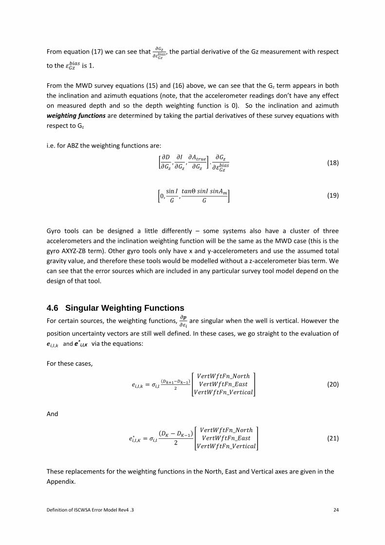
Definition of ISCWSA Error Model Rev4 .3 24
From equation (17) we can see that 𝜕𝐺𝑧
𝜕휀𝐺𝑧𝑏𝑖𝑎𝑠, the partial derivative of the Gz measurement with respect
to the 휀𝐺𝑧𝑏𝑖𝑎𝑠 is 1.
From the MWD survey equations (15) and (16) above, we can see that the Gz term appears in both
the inclination and azimuth equations (note, that the accelerometer readings don’t have any effect
on measured depth and so the depth weighting function is 0). So the inclination and azimuth
weighting functions are determined by taking the partial derivatives of these survey equations with
respect to Gz
i.e. for ABZ the weighting functions are:
[𝜕𝐷
𝜕𝐺𝑧
,𝜕𝐼
𝜕𝐺𝑧
,𝜕𝐴𝑡𝑟𝑢𝑒
𝜕𝐺𝑧
] .𝜕𝐺𝑧
𝜕휀𝐺𝑧𝑏𝑖𝑎𝑠
(18)
[0,
sin 𝐼
𝐺,𝑡𝑎𝑛Θ 𝑠𝑖𝑛𝐼 𝑠𝑖𝑛𝐴𝑚
𝐺] (19)
Gyro tools can be designed a little differently – some systems also have a cluster of three
accelerometers and the inclination weighting function will be the same as the MWD case (this is the
gyro AXYZ-ZB term). Other gyro tools only have x and y-accelerometers and use the assumed total
gravity value, and therefore these tools would be modelled without a z-accelerometer bias term. We
can see that the error sources which are included in any particular survey tool model depend on the
design of that tool.
4.6 Singular Weighting Functions
For certain sources, the weighting functions, 𝜕𝒑
𝜕𝜀𝑖 are singular when the well is vertical. However the
position uncertainty vectors are still well defined. In these cases, we go straight to the evaluation of
𝒆𝑖,𝑙,𝑘 and e*i,l,K via the equations:
For these cases,
𝑒𝑖,𝑙,𝑘 = 𝜎𝑖,𝑙(𝐷𝑘+1−𝐷𝑘−1)
2[
𝑉𝑒𝑟𝑡𝑊𝑓𝑡𝐹𝑛_𝑁𝑜𝑟𝑡ℎ𝑉𝑒𝑟𝑡𝑊𝑓𝑡𝐹𝑛_𝐸𝑎𝑠𝑡
𝑉𝑒𝑟𝑡𝑊𝑓𝑡𝐹𝑛_𝑉𝑒𝑟𝑡𝑖𝑐𝑎𝑙] (20)
And
𝑒𝑖,𝑙,𝐾
∗ = 𝜎𝑖,𝑙
(𝐷𝐾 − 𝐷𝐾−1)
2[
𝑉𝑒𝑟𝑡𝑊𝑓𝑡𝐹𝑛_𝑁𝑜𝑟𝑡ℎ𝑉𝑒𝑟𝑡𝑊𝑓𝑡𝐹𝑛_𝐸𝑎𝑠𝑡
𝑉𝑒𝑟𝑡𝑊𝑓𝑡𝐹𝑛_𝑉𝑒𝑟𝑡𝑖𝑐𝑎𝑙] (21)
These replacements for the weighting functions in the North, East and Vertical axes are given in the
Appendix.
Definition of ISCWSA Error Model Rev4 .3 25
4.7 Summation of Uncertainty Terms and Propagation Modes
The tool model for any particular survey instrument will include a number of different error sources,
and we must consider all survey legs in the well and all the survey stations in each leg. So for a well
we must add the error contributions over:
i. all survey legs in the well (index by l)
ii. each survey station in each leg (indexed by k)
iii. the contributions from each error source (indexed by i)
Once we have calculated the contribution to the error ellipse from each error source, at each survey
station in each leg of our well, we have to add up all these contributions. However, when doing this
we have to take into account how the errors relate to each other at station and hence how the
uncertainty values should be accumulated.
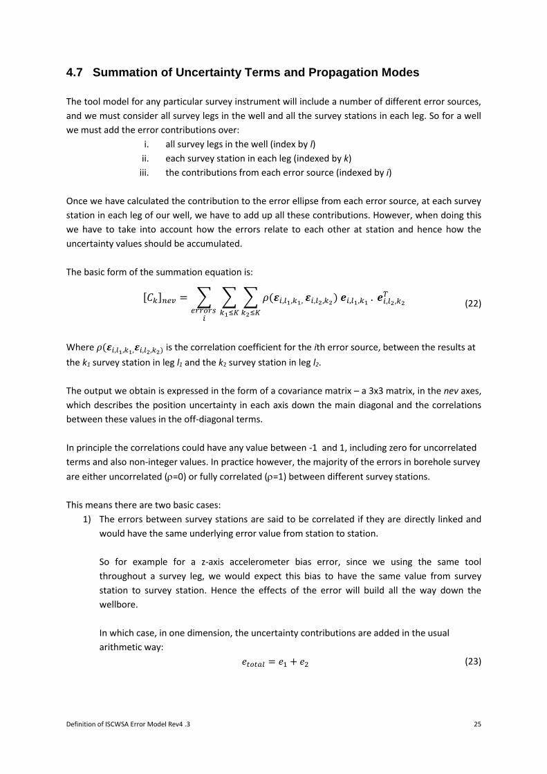
The basic form of the summation equation is:
[𝐶𝑘]𝑛𝑒𝑣 = ∑ ∑ ∑ 𝜌(𝜺𝑖,𝑙1,𝑘1,
𝑘2≤𝐾
𝜺𝑖,𝑙2,𝑘2) 𝒆𝑖,𝑙1,𝑘1 . 𝒆𝑖,𝑙2,𝑘2
𝑇
𝑘1≤𝐾𝑒𝑟𝑟𝑜𝑟𝑠
𝑖
(22)
Where 𝜌(𝜺𝑖,𝑙1,𝑘1,𝜺𝑖,𝑙2,𝑘2) is the correlation coefficient for the ith error source, between the results at
the k1 survey station in leg l1 and the k2 survey station in leg l2.
The output we obtain is expressed in the form of a covariance matrix – a 3x3 matrix, in the nev axes,
which describes the position uncertainty in each axis down the main diagonal and the correlations
between these values in the off-diagonal terms.
In principle the correlations could have any value between -1 and 1, including zero for uncorrelated
terms and also non-integer values. In practice however, the majority of the errors in borehole survey
are either uncorrelated (=0) or fully correlated (=1) between different survey stations.
This means there are two basic cases:
1) The errors between survey stations are said to be correlated if they are directly linked and
would have the same underlying error value from station to station.
So for example for a z-axis accelerometer bias error, since we using the same tool
throughout a survey leg, we would expect this bias to have the same value from survey
station to survey station. Hence the effects of the error will build all the way down the
wellbore.
In which case, in one dimension, the uncertainty contributions are added in the usual
arithmetic way:
𝑒𝑡𝑜𝑡𝑎𝑙 = 𝑒1 + 𝑒2 (23)
Definition of ISCWSA Error Model Rev4 .3 26
2) If the errors are not linked from station to station then they are uncorrelated or statistically
independent, e.g. if we have two independent error sources, then they could both cause a
positive inclination error and add together but it is also possible that one might create a
positive inclination error and the other a negative error.
In which case we are taking a random value from pot 1 and a random value from pot 2 and
the error contributions must be root sum squared (RSS) together:
𝑒𝑡𝑜𝑡𝑎𝑙 = √𝑒1
2 + 𝑒22 (24)
It is a basic assumption of the model framework that the statistics of the various different error
sources are independent so they will be RSS’d together – for example, there is no reason why sag
error would be connected to z-axis magnetometer bias or to declination error etc. [This is the
reason why ԑI is not split into ԑI1 and ԑI2 in Eq. 21; the correlation ρ(ԑI1, ԑI2) is by assumption always 0
between different sources i1 and i2.]
Although the different error sources are independent from each other an individual error source
may or may not be statistical correlated from survey to survey along the well.
The possible correlation between measurements depends as much on the tool configuration and
measurement mode, as on the error source itself. For example, the z-axis magnetometer bias may
be persistent for a particular surveying tool, and hence give correlated readings throughout a survey
leg. However, if we go to another leg, using a different tool, the effect of this bias should not be
correlated between the two legs. Similarly, an error source may behave correlated between survey
legs in the same well, but independent between survey legs in different wells. The “lowest degree”
of correlation occurs when any two measurements are independent, in which case the error source
is termed random.
So a given error source may be independent at all surveys stations, or correlated between survey
station- either just the stations within a leg, or over all legs within a well or over all wells within a
field.
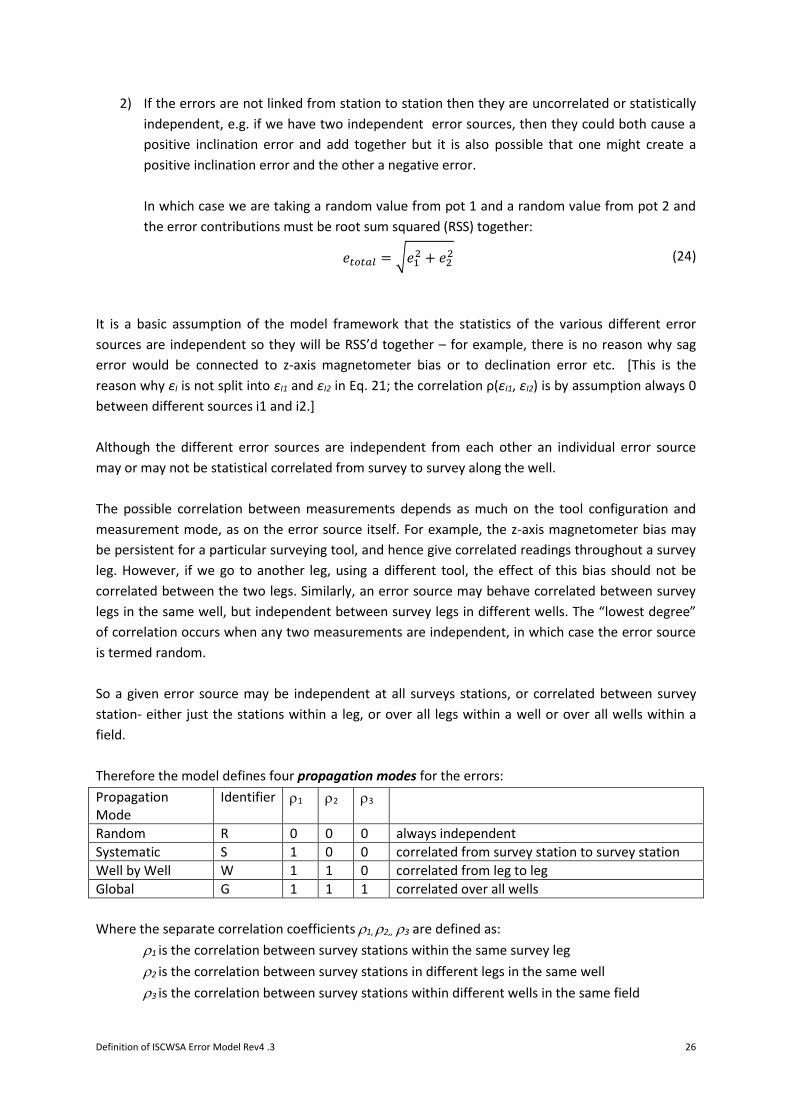
Therefore the model defines four propagation modes for the errors:
Propagation Mode
Identifier 1 2 3
Random R 0 0 0 always independent
Systematic S 1 0 0 correlated from survey station to survey station
Well by Well W 1 1 0 correlated from leg to leg
Global G 1 1 1 correlated over all wells
Where the separate correlation coefficients 1, 2,, 3 are defined as:
1 is the correlation between survey stations within the same survey leg
2 is the correlation between survey stations in different legs in the same well
3 is the correlation between survey stations within different wells in the same field
Definition of ISCWSA Error Model Rev4 .3 27
The propagation mode is a property of the error source and is defined in the tool model. In practice,
most error sources are systematic within a leg or are random and only a limited number of well by
well or global sources have been identified.
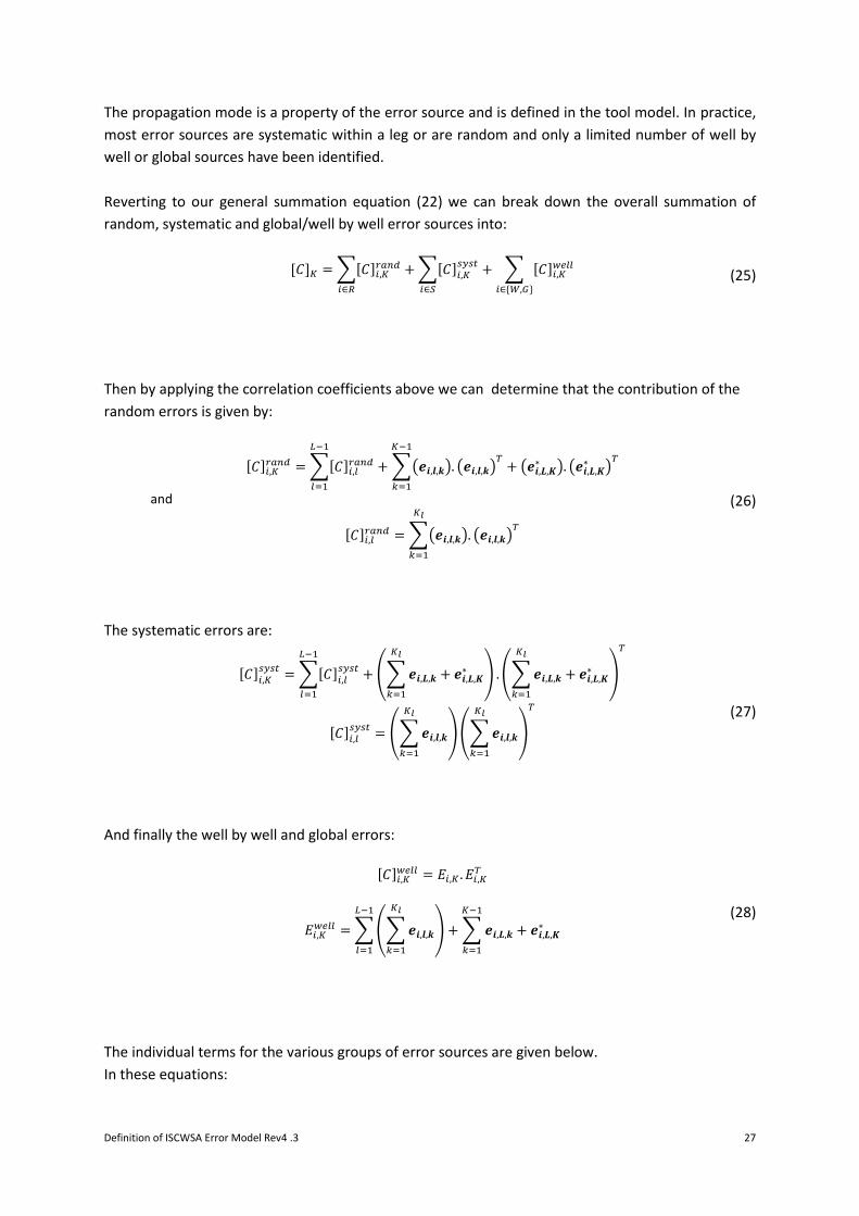
Reverting to our general summation equation (22) we can break down the overall summation of
random, systematic and global/well by well error sources into:
[𝐶]𝐾 = ∑[𝐶]𝑖,𝐾𝑟𝑎𝑛𝑑
𝑖∈𝑅
+ ∑[𝐶]𝑖,𝐾𝑠𝑦𝑠𝑡
𝑖∈𝑆
+ ∑ [𝐶]𝑖,𝐾𝑤𝑒𝑙𝑙
𝑖∈{𝑊,𝐺}
(25)
Then by applying the correlation coefficients above we can determine that the contribution of the
random errors is given by:
[𝐶]𝑖,𝐾𝑟𝑎𝑛𝑑 = ∑[𝐶]𝑖,𝑙
𝑟𝑎𝑛𝑑
𝐿−1
𝑙=1
+ ∑(𝒆𝒊,𝒍,𝒌). (𝒆𝒊,𝒍,𝒌)𝑇
+ (𝒆𝒊,𝑳,𝑲∗ ). (𝒆𝒊,𝑳,𝑲
∗ )𝑇
𝐾−1
𝑘=1
and
[𝐶]𝑖,𝑙𝑟𝑎𝑛𝑑 = ∑(𝒆𝒊,𝒍,𝒌). (𝒆𝒊,𝒍,𝒌)
𝑇
𝐾𝑙
𝑘=1
(26)
The systematic errors are:
[𝐶]𝑖,𝐾𝑠𝑦𝑠𝑡
= ∑[𝐶]𝑖,𝑙𝑠𝑦𝑠𝑡
𝐿−1
𝑙=1
+ (∑ 𝒆𝒊,𝑳,𝒌 + 𝒆𝒊,𝑳,𝑲∗
𝐾𝑙
𝑘=1
) .(∑ 𝒆𝒊,𝑳,𝒌 + 𝒆𝒊,𝑳,𝑲∗
𝐾𝑙
𝑘=1
)
𝑇
[𝐶]𝑖,𝑙𝑠𝑦𝑠𝑡
= (∑ 𝒆𝒊,𝒍,𝒌
𝐾𝑙
𝑘=1
)(∑ 𝒆𝒊,𝒍,𝒌
𝐾𝑙
𝑘=1
)
𝑇
(27)
And finally the well by well and global errors:
[𝐶]𝑖,𝐾
𝑤𝑒𝑙𝑙 = 𝐸𝑖,𝐾 . 𝐸𝑖,𝐾𝑇
𝐸𝑖,𝐾𝑤𝑒𝑙𝑙 = ∑(∑ 𝒆𝒊,𝒍,𝒌
𝐾𝑙
𝑘=1
)
𝐿−1
𝑙=1
+ ∑ 𝒆𝒊,𝑳,𝒌 + 𝒆𝒊,𝑳,𝑲∗
𝐾−1
𝑘=1
(28)
The individual terms for the various groups of error sources are given below.
In these equations:

Definition of ISCWSA Error Model Rev4 .3 28
ei,l,k is the vector contribution of ith error source, in the ith survey leg at the kth survey
station (3x1 vector)
e*i,l,K is the vector contribution of ith error source, in the ith survey leg at the last survey
point of interest i.e. the Kth survey station (3x1 vector)
i is the summation over error sources from 1…I
k is the summation of survey stations from 1…K: the current survey station
l is the summation over survey legs from 1..L: the current survey leg
The mathematical details of this process can be found in Appendix A.
The final output of the summation is a 3x3 covariance matrix, which describes the error ellipse at a
particular station. In the nev-axes, the covariance matrix is:
[𝐶]𝑛𝑒𝑣 = [
𝜎𝑁2 𝐶𝑜𝑣(𝑁, 𝐸) 𝐶𝑜𝑣(𝑁, 𝑉)
𝐶𝑜𝑣(𝑁, 𝐸) 𝜎𝐸2 𝐶𝑜𝑣(𝐸, 𝑉)
𝐶𝑜𝑣(𝑁, 𝑉) 𝐶𝑜𝑣(𝐸, 𝑉) 𝜎𝑉2
] (29)
Here 𝜎𝑁2 is the variance in the north-axis and the uncertainty in north axis (at 1-standard deviation) is
±√𝜎𝑁2 .
In the same way, the other terms on the lead diagonal are uncertainties along the other principle
axes. The 𝐶𝑜𝑣(𝑁, 𝐸), 𝐶𝑜𝑣(𝑁, 𝑉) and 𝐶𝑜𝑣(𝐸, 𝑉) terms are the covariances and give the skew or
rotation of the ellipse with respect to the principle axes.
4.8 Transformation to Borehole Axes
The covariance matrix above is expressed in the earth-centred nev-axes, this can be transformed to
the borehole reference frame, hla by pre- and post-multiplying the covariance matrix with the nev-
to-hla direction cosine matrix, [𝑇]ℎ𝑙𝑎𝑛𝑒𝑣.
[𝐶]ℎ𝑙𝑎 = [𝑇]ℎ𝑙𝑎𝑛𝑒𝑣𝑇
[𝐶]𝑛𝑒𝑣[𝑇]ℎ𝑙𝑎𝑛𝑒𝑣 (30)
The direction cosine matrix can be obtained a rotation in the horizontal place to the borehole
azimuth, followed by a rotation in the vertical to the borehole inclination and is given by:
[𝑇]ℎ𝑙𝑎𝑛𝑒𝑣 = [
𝑐𝑜𝑠𝐼𝑐𝑜𝑠𝐴 −𝑠𝑖𝑛𝐴 𝑠𝑖𝑛𝐼𝑐𝑜𝑠𝐴𝑐𝑜𝑠𝐼𝑠𝑖𝑛𝐴 𝑐𝑜𝑠𝐴 𝑠𝑖𝑛𝐼𝑠𝑖𝑛𝐴−𝑠𝑖𝑛𝐼 0 𝑐𝑜𝑠𝐼
] (31)

Definition of ISCWSA Error Model Rev4 .3 29
4.9 Position Uncertainty Model for a Specific Tool
The elements required to model a specific survey tool are:
1) The error sources which are defined for the tool (generally each source has an identifier,
although this is not strictly essential).
2) The magnitude for each error source.
3) The units for that magnitude.
4) The propagation mode for each source.
5) The weighting functions to be invoked for depth, inclination and azimuth errors (either
specified as formulae or by reference).
6) Optionally, the inclination range over which that source is to be applied.
7) Optionally, design parameters to be used in the evaluation (e.g. running speed or cant angle
for certain gyro tools).
These items are often grouped together in what can be referred to as either a Position Uncertainty
Model (PUM), Instrument Performance Model (IPM), tool code, IPM file or error model.
The PUM will generally have a name to identify which survey tool is models and may also include
metadata such as revision number, comments on usage and applicability, and audit history
(originator, source, status, tool type etc.)
Since most tool codes can be created in fixed or floating platform versions, with varying depth
source magnitudes, some software now includes both sets of terms in the PUM and allows the
software to select the correct depth terms to apply, depending how the site for that well is setup.
Users should be aware of this complication if copying PUMs, since using all depth terms will result in
errors.

Definition of ISCWSA Error Model Rev4 .3 30
5 Error Sources and Weighting Functions
5.1 Common Elements of Modelling
Although many of the components of the MWD and gyro models are necessarily quite different, the
error sources which model depth and misalignment of the tool are the same. By this we mean that
the mathematical formulae are the same, but obviously actually magnitudes in the PUM will depend
on how a depth is obtained (e.g. wireline or pipe tally) and how a tool is centralised.
5.1.1 Depth Terms
Depth is covered with a reference term (which may be random or systematic), a scale and a stretch
term. Depth errors are discussed in further detail in [3].
The same weighting functions are used for gyro depth errors. In general most PUMs can be created
in two basic variants to cover the cases of surveys from a fixed rig (e.g. land rig) and from a floating
platform. The depth reference terms vary between these cases.
For example, the generic MWD models use the following values for modelling drill-pipe depth in
these two scenarios:
Error Source
Propagation Mode Units Fixed Floating
Depth: Depth Reference – Random DREF R m
2.2
Depth: Depth Reference – Systematic DREF S m
0.35 1
Depth: Depth Scale Factor – Systematic DSF S -
0.00056 0.00056
Depth: Depth Stretch – Global DST G 1/m
2.5E-07 2.5E-07
5.1.2 Borehole Misalignments
Borehole misalignments are handled in the same way in both the MWD and gyro models. This
method avoids the complication of toolface dependency in the misalignments which was present in
early versions and is considered to handle certain geometries, such helix-shaped, vertical boreholes
better than the original MWD terms. There are four borehole error source terms and three possible
calculation options which are handled via two weight parameters.
The full range of options is given by
Weighting Functions
Error Source Depth Inclination Azimuth
XYM1 0 w12 0
XYM2 0 0 w12/sin(I)
XYM3 0 w34 cos(At) - w34 sin(At)) / sin(I)
XYM4 0 w34 sin(At) w34 cos(At)) / sin(I)
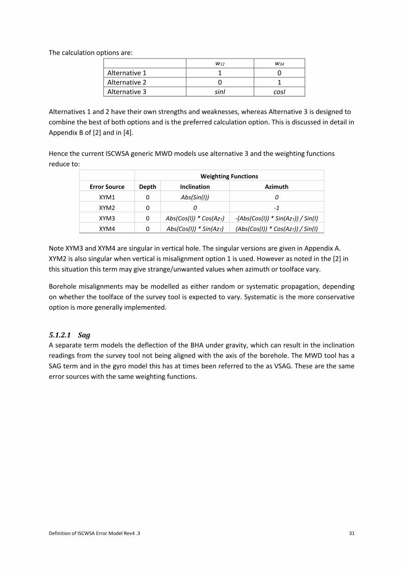
Definition of ISCWSA Error Model Rev4 .3 31
The calculation options are:
w12 w34
Alternative 1 1 0
Alternative 2 0 1
Alternative 3 sinI cosI
Alternatives 1 and 2 have their own strengths and weaknesses, whereas Alternative 3 is designed to
combine the best of both options and is the preferred calculation option. This is discussed in detail in
Appendix B of [2] and in [4].
Hence the current ISCWSA generic MWD models use alternative 3 and the weighting functions
reduce to:
Weighting Functions
Error Source Depth Inclination Azimuth
XYM1 0 Abs(Sin(I)) 0
XYM2 0 0 -1
XYM3 0 Abs(Cos(I)) * Cos(AzT) -(Abs(Cos(I)) * Sin(AzT)) / Sin(I)
XYM4 0 Abs(Cos(I)) * Sin(AzT) (Abs(Cos(I)) * Cos(AzT)) / Sin(I)
Note XYM3 and XYM4 are singular in vertical hole. The singular versions are given in Appendix A.
XYM2 is also singular when vertical is misalignment option 1 is used. However as noted in the [2] in
this situation this term may give strange/unwanted values when azimuth or toolface vary.
Borehole misalignments may be modelled as either random or systematic propagation, depending
on whether the toolface of the survey tool is expected to vary. Systematic is the more conservative
option is more generally implemented.
5.1.2.1 Sag
A separate term models the deflection of the BHA under gravity, which can result in the inclination
readings from the survey tool not being aligned with the axis of the borehole. The MWD tool has a
SAG term and in the gyro model this has at times been referred to the as VSAG. These are the same
error sources with the same weighting functions.
Definition of ISCWSA Error Model Rev4 .3 32
6 MWD Modelling
In general ISCWSA does not generate position uncertainty models for particular survey tools.
The exception to this rule, are the models for generic MWD tools, for which does ISCWSA does
define eight PUMs. These cover the various combinations of uncorrected and axial-corrected MWD,
in fixed and floating platform variants, with and without sag correction. The error model
maintenance committee does not create PUMs for any further MWD variants (such as IFR1, multi-
station versions etc.)
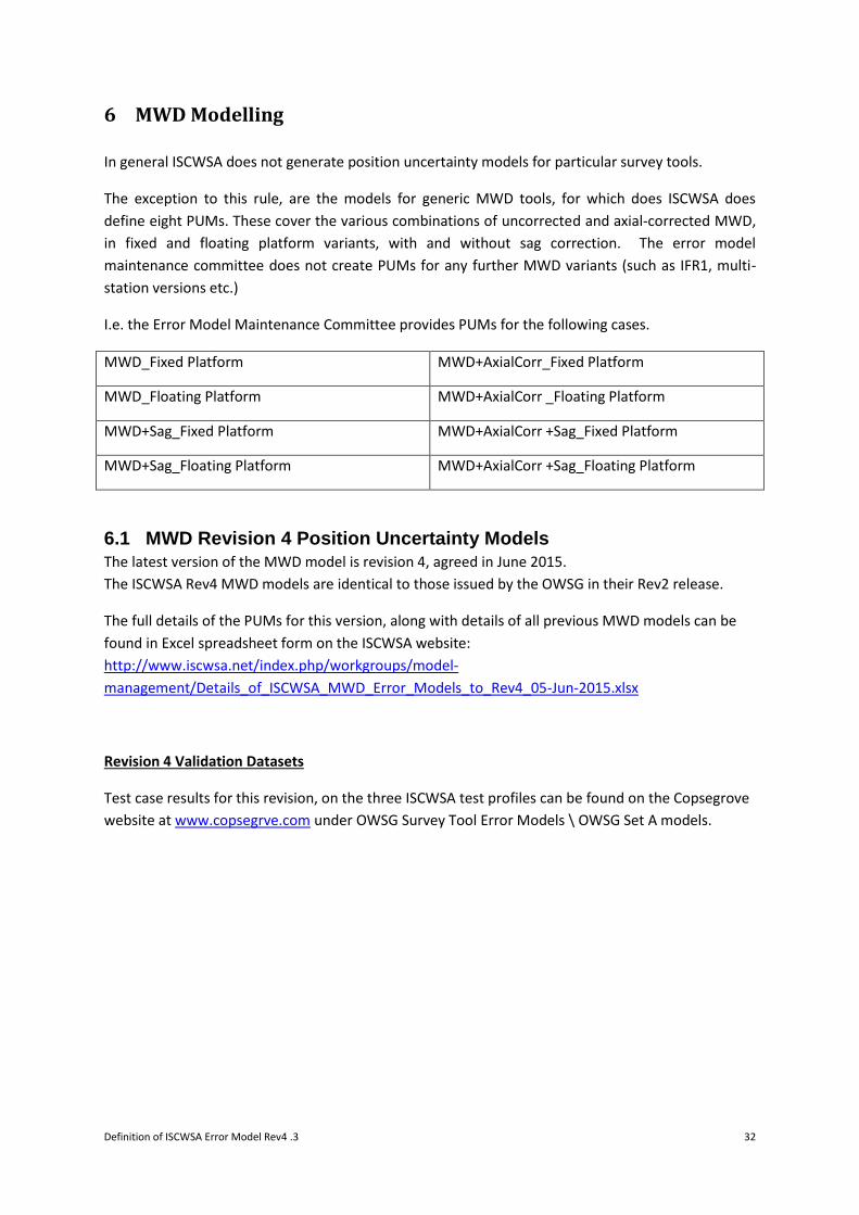
I.e. the Error Model Maintenance Committee provides PUMs for the following cases.
MWD_Fixed Platform MWD+AxialCorr_Fixed Platform
MWD_Floating Platform MWD+AxialCorr _Floating Platform
MWD+Sag_Fixed Platform MWD+AxialCorr +Sag_Fixed Platform
MWD+Sag_Floating Platform MWD+AxialCorr +Sag_Floating Platform
6.1 MWD Revision 4 Position Uncertainty Models
The latest version of the MWD model is revision 4, agreed in June 2015.
The ISCWSA Rev4 MWD models are identical to those issued by the OWSG in their Rev2 release.
The full details of the PUMs for this version, along with details of all previous MWD models can be
found in Excel spreadsheet form on the ISCWSA website:
http://www.iscwsa.net/index.php/workgroups/model-
management/Details_of_ISCWSA_MWD_Error_Models_to_Rev4_05-Jun-2015.xlsx
Revision 4 Validation Datasets
Test case results for this revision, on the three ISCWSA test profiles can be found on the Copsegrove
website at www.copsegrve.com under OWSG Survey Tool Error Models \ OWSG Set A models.
Definition of ISCWSA Error Model Rev4 .3 33
6.2 Weighting Functions
The revision 4 model contains 34 weighting functions:
4 depth terms 4 borehole misalignment terms 1 sag term 20 terms for bias and scalefactor errors on the sensors 4 terms for reference field errors 1 drillstring interference term.
Details of all of the weighting functions can be found in the appendix to this document and also in
the spreadsheet referenced above which details the PUMs.
6.2.1 Sensor Terms
The model includes bias and scalefactor errors for all the sensors in the tool. Since revision 3, these
are modelled using toolface independent weighting functions following the methodology described
in [13]. This combines the x and y axis sensor terms which end up being represented by two biases
and three scalefactors for the accelerometers and a similar number for the magnetometers. The
axial terms remain as a single bias and scalefactor for the z-accelerometer and z-magnetometer. This
is a total of fourteen sensor terms.
The model covers both the variations of standard MWD and MWD with an axial magnetic
interference correction (so called short-collar or single station corrections.). This results in a
complete second set of sensor error terms. Only one set of sensor terms will be valid for any given
situation.
For each sensor type, one of the scalefactor terms always propagates and systematic but the
remainder may propagate as random or systematic depending on whether sliding or rotating drilling
is modelled. In practise, the more conservative option of systematic propagation is generally used
and that is what is quoted in the published ISCWSA PUMs.
Note that two of the cross axial accelerometer terms are singular in vertical hole, the modified
version of the weighting functions are also given. Chad Hanak has produced a document which
describes in the detail the derivation of the singular terms for the various versions of the error
model [10].
6.2.2 Drillstring Interference
MWD users should model the expected magnetic interference from the BHA and hence determine
suitable non-magnetic spacing distances. Revision 4 assumes that the BHA is spaced in this way to
within a specified amount of magnetic interference in nT. There is now one term, AMIL which
models drillstring interference. In the generic models this level is assumed to be 220nT at 1-sigma.
Definition of ISCWSA Error Model Rev4 .3 34
6.2.3 Geo-magnetic Reference
Two error sources are included for declination error (two sources one constant and one proportional
to the horizontal component of the Earth’s field) and one each for total field and dip. The total field
and dip terms are only used in axially corrected models.
The latest revisions include both systematic and random versions of all geo-magnetic terms. The
random terms have relatively little impact on the ellipse sizes but are included for consistency and
for use when deriving implied QA\QC limits.
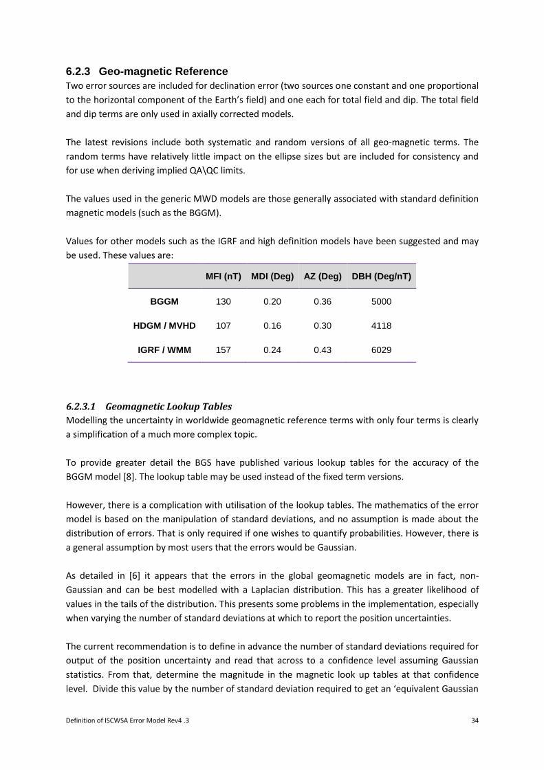
The values used in the generic MWD models are those generally associated with standard definition
magnetic models (such as the BGGM).
Values for other models such as the IGRF and high definition models have been suggested and may
be used. These values are:
MFI (nT) MDI (Deg) AZ (Deg) DBH (Deg/nT)
BGGM 130 0.20 0.36 5000
HDGM / MVHD 107 0.16 0.30 4118
IGRF / WMM 157 0.24 0.43 6029
6.2.3.1 Geomagnetic Lookup Tables
Modelling the uncertainty in worldwide geomagnetic reference terms with only four terms is clearly
a simplification of a much more complex topic.
To provide greater detail the BGS have published various lookup tables for the accuracy of the
BGGM model [8]. The lookup table may be used instead of the fixed term versions.
However, there is a complication with utilisation of the lookup tables. The mathematics of the error
model is based on the manipulation of standard deviations, and no assumption is made about the
distribution of errors. That is only required if one wishes to quantify probabilities. However, there is
a general assumption by most users that the errors would be Gaussian.
As detailed in [6] it appears that the errors in the global geomagnetic models are in fact, non-
Gaussian and can be best modelled with a Laplacian distribution. This has a greater likelihood of
values in the tails of the distribution. This presents some problems in the implementation, especially
when varying the number of standard deviations at which to report the position uncertainties.
The current recommendation is to define in advance the number of standard deviations required for
output of the position uncertainty and read that across to a confidence level assuming Gaussian
statistics. From that, determine the magnitude in the magnetic look up tables at that confidence
level. Divide this value by the number of standard deviation required to get an ‘equivalent Gaussian
Definition of ISCWSA Error Model Rev4 .3 35
standard deviation’ (valid only at the confidence level in question) and then use that value as normal
in the subsequent error model calculations. In that way, when the error model results are scaled
back up to the required number of standard deviations, the geomagnetic terms will be reported at
the correct confidence level.
That is, if reporting ellipses at 2 standard deviations (95.4% confidence in one dimensional Gaussian
distributions), utilise the 95.4% look up table, read of the error source magnitudes at the given
latitude and longitude of the well site. Divide those numbers by 2 to get the standard deviations to
obtain an equivalent error source magnitude for use in the calculations.
Currently, the lookup tables are optional and are not considered as a revision of the model.
6.3 History of the MWD Error Model
There have been several revisions to the MWD error model over the years. Concise details of all the
versions may be found in Excel spreadsheet form on the Error Model Management Group webpage
as given in the previous section. This page will give a brief overview of the changes:
The revisions to the MWD Error Model are:
Rev 0 As per SPE 67616 together with a number of typographical corrections [4]
Rev 1 Changed to the gyro style misalignment with 4 terms and calculation options [4]
Rev 2 Changes to the parameter values for the depth scale and stretch terms [4]
Rev 3 Replacement of all toolface dependant terms. [5]
Rev 4 Introduction of AMIL term and changes to misalignment magnitudes. Random magnetic reference values introduced to the main MWD model
6.3.1 Revision 0
The MWD error model was originally published as SPE 56702 in October 1999. This paper was
updated and was published in SPE Drilling and Completion as SPE 67616 [1], in December 2000. The
paper covers three distinct areas. It lays out the framework of the ISCWSA error model as discussed
in the previous section, it defines the error sources applicable to MWD tools and it provides error
magnitudes for these values, complete with a technical justification.
After, the publication of the SPE 67616, a small number of typographical errors identified and
corrected and this defined as revision 0.
6.3.2 Revision 1
This revision changed how borehole misalignments were handled in the MWD model by adopting
the same methodology as defined for the gyro model in [2]. The existing MX and MY misalignments
were deprecated and replaced with the XYM1, XYM2, XYM3, XYM4 sources described above.
Definition of ISCWSA Error Model Rev4 .3 36
6.3.3 Revision 2
Revision 2 made changes to the various depth error magnitudes for both fixed and floating
platforms. The consensus of the committee was that the previous depth terms were incorrect.
6.3.4 Revision 3
Rev3 replaced the 16 toolface dependant weighting functions with 20 new ones, following a method
developed for the gyro error model. This removes the need to either include survey toolface, or to
use methods to evaluate at the planning stage which tool-faces might be observed, a process which
can give rise to unexpected results.
The new terms replace all the existing x and y accelerometer and x and y magnetometer bias and
scalefactor terms, for both the standard MWD and MWD with axial correction cases. The suffix
_TI1, _TI2 etc. is often used to differentiate these terms from the Rev2 sensor terms, where TI1
stands to Toolface Independent source 1 etc.
The new terms pull together the x and y effects, and the propagation mode varies from either
random, where the toolface varies between survey stations and systematic for sliding between
survey stations with constant toolface. In practise for MWD the random propagation would not
normally be considered at the planning stage. The details of revision 3 are dealt with in [5].
6.3.5 Revision 4
Changes in revision 4:
1) The magnitudes of the borehole misalignment terms were increased from 0.06 deg to 0.1 deg.
This change was implemented because, after consideration, the group felt that the existing
values were too optimistic particularly in top hole. Hence ellipse sizes can be expected to be
larger in top hole.
2) Replacement of the existing AMID and AMIC drillstring interference terms (which had units in
degrees) with the AMIL term (which is specified in nano-Tesla). This reflects a change in how
many companies do their non-mag spacing calculations. The older terms followed the
philosophy in SPE67616, “A well-established industry practice is to require nonmagnetic spacing
sufficient to keep the azimuth error below a fixed tolerance, typically ~0.5° at 1 s.d. for assumed
pole strengths and a given hole direction. This tolerance may need to be compromised in the
least favourable hole directions.” The use of the AMIL term assumes that BHA’s are designed
with a specific length of non-mag and hence a consistent level of expected drillstring magnetic
interference. The effect that this magnetic interference has on azimuth will then vary
dependant on the well inclination, azimuth and the horizontal component of the Earth’s
magnetic field. For the same BHA, large angular errors can be expected at higher latitudes. A
magnitude of 220nT was chosen for AMIL, as a reasonable generic value. This gives reasonable
agreement to the old model at mid-latitudes. However, the behaviour of the AMIL term is
inherently different to AMIC+AMID and hence the error model will give different results
depending on the well orientation and location.

Definition of ISCWSA Error Model Rev4 .3 37
3) Addition of DECR, DBHR, MDIR and MFIR terms to model random fluctuations in the
geomagnetic reference field for declination, total field and dip. These terms were added for
consistency with some of the commonly used IFR models. They will have a limited effect on the
ellipse sizes, but will influence any field acceptance criteria derived from the error model values.
6.3.6 Bias Models
Early revision of the model included biased terms for depth and drill string interference terms.
It is well recognised that using drill pipe measurements on surface and the driller’s tally results in an
underestimate of the true wellbore measured depth, since drill pipe will stretch due the suspended
weight and will expand as temperature increases in hole. Similarly there has been some evidence
that drill string interference terms are not completely random. Therefore bias terms were included
in the model which had the effect of moving the centre of the survey ellipses away from the
recorded survey station.
From revision 3 onwards ISCWSA advice was that bias model should not be used. They tend to
confuse users and if the size of the bias error is significant for a survey application the
recommendation would be to actually correct for the bias (with depth or interference corrections)
rather than to move the ellipses.
Therefore from revision 3 bias terms have been deprecated.
Definition of ISCWSA Error Model Rev4 .3 38
7 Gyro Models
The core mathematics of the gyro model is designed to be independent of the technology used and
it should be capable of modelling all systems currently in use or which have been foreseen. As
before the specifics for a given tool/technology are contained in the specific error sources,
magnitudes and propagation modes defined in the position uncertainty model for that tool.
Unlike MWD tools, which generally have a similar sensor configuration, gyro survey tools come in
various different designs and can operate in two different ways. This means that although the basic
ISCWSA framework is still used for modelling gyro tools the details of the models are more
complicated and some additional features are needed.
The additional considerations are differing sets of weighting functions depending on the sensor
configuration and two operating modes – stationary and continuous mode – with the model
transitioning between these modes at defined inclinations.
In stationary (or gyro-compassing mode), the gyro is held at a fixed point in the borehole and the
sensor readings as used to determine the inclination and azimuth of the tool relative to the Earth’s
axis of rotation. An independent assessment of the inclination and azimuth is made at each survey
station and depth may come from wireline or pipe tally.
In continuous mode the gyro is first initialised to define it’s inclination and azimuth and then the
gyro sensors record changes to that initial orientation to attitude at subsequent points. Therefore all
the later azimuths are dependent on the initial heading value. That initial azimuth may come from a
stationary gyro-compass or made be defined by the user from an external reference source.
In such a case, a system may use stationary mode when near vertical and then switch over to
continuous mode once the inclination builds above a set value. It is possible for the tool to move
back to gyro-compassing mode if the hole angle drops again.
Stationary gyro mode is quite similar to the way in which MWD operates, and, aside from different
weighting, functions the model behaves in a similar way. Weighting functions are evaluated at each
station as a function of the depth, inclination, azimuth and some reference parameters (such as
latitude). However, it should be noted that the weighting functions depend on TRUE azimuth and
not MAGNETIC azimuth as in the MWD case.
Continuous mode is quite different as the weighting functions at each station are evaluated
recursively i.e. they are dependent on their value at the previous survey station.
Definition of ISCWSA Error Model Rev4 .3 39
7.1 Sensor Configuration
Nearly all MWD tools consist of three orthogonal accelerometers and three orthogonal
magnetometers.
However gyro tools can be built with various sensor configurations, with two or three
accelerometers and with one, two or three gyros. The sensor configuration influences the navigation
equations and hence there are different weighting functions in each case.
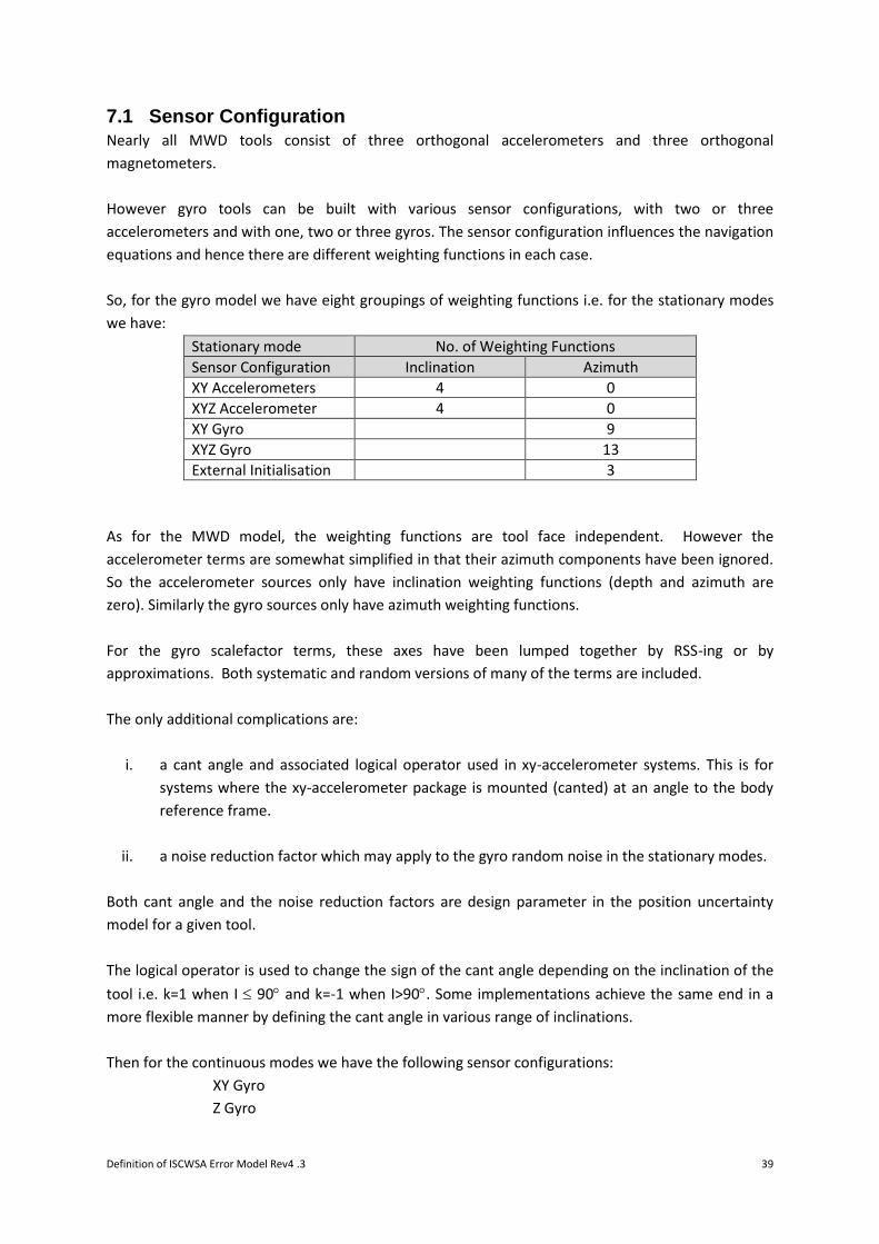
So, for the gyro model we have eight groupings of weighting functions i.e. for the stationary modes
we have:
Stationary mode No. of Weighting Functions
Sensor Configuration Inclination Azimuth
XY Accelerometers 4 0
XYZ Accelerometer 4 0
XY Gyro 9
XYZ Gyro 13
External Initialisation 3
As for the MWD model, the weighting functions are tool face independent. However the
accelerometer terms are somewhat simplified in that their azimuth components have been ignored.
So the accelerometer sources only have inclination weighting functions (depth and azimuth are
zero). Similarly the gyro sources only have azimuth weighting functions.
For the gyro scalefactor terms, these axes have been lumped together by RSS-ing or by
approximations. Both systematic and random versions of many of the terms are included.
The only additional complications are:
i. a cant angle and associated logical operator used in xy-accelerometer systems. This is for
systems where the xy-accelerometer package is mounted (canted) at an angle to the body
reference frame.
ii. a noise reduction factor which may apply to the gyro random noise in the stationary modes.
Both cant angle and the noise reduction factors are design parameter in the position uncertainty
model for a given tool.
The logical operator is used to change the sign of the cant angle depending on the inclination of the
tool i.e. k=1 when I 90 and k=-1 when I>90. Some implementations achieve the same end in a
more flexible manner by defining the cant angle in various range of inclinations.
Then for the continuous modes we have the following sensor configurations:
XY Gyro
Z Gyro
Definition of ISCWSA Error Model Rev4 .3 40
XYZ Gyro
each configuration has two weighting functions, one for a gyro drift term and the second a gyro
random walk term.
Depending on the tool configuration the appropriate group of weighting functions would be invoked
in each mode, although not all of the weighting functions in the group may be used. So a stationary
tool PUM might have XYZ Accel and XY Gyro weighting functions. We would not expect to see
weighting functions from both the XYZ Accel and XY Accel group in the same PUM. We do
sometimes see XY Accel, XY Static, Z Continuous Gyro and XY Continuous Gyro all in the one PUM.
All the required weighting functions are listed in the Appendix. Derivations of the weighting
functions can be found in [2].
ISCWSA does not define any gyro models for use.
7.2 Operating Modes
As outlined above, the gyro model considers two distinct operating modes for the tool.
Firstly, stationary mode is quite similar to the MWD model, where the weighting functions are
evaluated at each survey station based purely on the current measured depth, inclination and
azimuth and the physical details of the reference field – the total gravity value, the latitude and the
constant of Earth’s rotation etc.
However, now a continuous mode is also introduced. In continuous mode, weighting functions are
evaluated recursively i.e. the new value of a weighting function depends on the value it had at the
previous survey station plus and additional increment.
In reality the sources that are important in continuous mode cause the attitude errors to build over
time. In order to have a means of estimating elapsed time between surveys we evaluate the change
in measured depth divided by the tool running speed. This running speed is another tool design
parameter, which is defined in the position uncertainty model, along with the tool magnitudes.
Continuous mode weighting functions are written in the form:
ℎ𝑖 = ℎ𝑖−1 +
∆𝐷𝑖
𝑐 (32)
Where hi is the new value of the weighting function, hi-1 is the value of this weighting function at the
previous survey station, ∆𝐷𝑖 is the change in depth between the two stations and the c is the
running speed.
Definition of ISCWSA Error Model Rev4 .3 41
As a distance divided by speed, ∆𝐷𝑖
𝑐 has units of time. Evaluation of this term should be such that the
time units match the biases and random walks (most often defined in deg/hr and deg/hr
respectively). Similarly, obvious the units for D and c must match (m and m/hr or ft and ft/hr).
The transition from stationary to continuous mode is considered to occur at a given inclination. So in
the gyro model the sources now have a specified inclination range in which to be evaluated.
Before the transition inclination, the tool with operate in stationary mode and the weighting
functions evaluated as normal. The weighting functions for the continuous sources are zero at this
point.
After the transition the continuous weighting functions are evaluated. However, the azimuth
uncertainty accumulated in the stationary sources is still required, since the subsequent azimuth
measurements depend on the value at transition. Therefore either the stationary weighting
functions are ‘frozen’ so they continue to give the same values throughout the continuous running,
or the total azimuth error at transition can be moved into the EXT-INIT term. Note also that at
transition any random gyro source which are frozen should change to systematic propagation for the
remainder of that survey leg.
To put this in context, a given tool may be initialised in the stationary mode and transition to
continuous mode once the hole inclination builds above 15. All the surveys before the transition are
stationary surveys, and the PUM will define the appropriate stationary functions to use. At transition
to continuous mode the total azimuth uncertainty from all the stationary sources is 0.6, via
∑ 𝜎𝑖,𝐿
𝜕𝐴𝑧𝑲
𝜕휀𝑖𝑖∈𝑠𝑡𝑎𝑡𝑖𝑜𝑛𝑎𝑟𝑦 𝑔𝑦𝑟𝑜 𝑠𝑜𝑢𝑟𝑐𝑒𝑠
(33)
After transition, the stationary sources are all frozen so that they continue to give an azimuth error
of 0.6. However, the error vector, e, due to these sources will of course change since although the
outer terms are fixed, the geometry term in the brackets in equation (6) will vary at the subsequent
stations.
𝒆𝑖,𝑙,𝑘 = 𝜎𝑖,𝑙 (
𝑑∆𝒓𝑘
𝑑𝒑𝑘
+𝑑∆𝒓𝑘+1
𝑑𝒑𝑘
)𝜕𝒑𝑘
𝜕휀𝑖
(6)
In addition to these stationary sources, the continuous terms will also come into play. The
accelerometer terms, which determine the inclination uncertainty, are evaluated as stationary terms
throughout.
If the tool were to drop back below 15, the tool would drop back into stationary mode. In which
case the model behaves in stationary mode exactly as before. The stationary weighting functions
would be ‘unfrozen’ and evaluated as normal and the continuous weighting functions would be zero.

Definition of ISCWSA Error Model Rev4 .3 42
To stop unnecessary switching back and forward between modes (as might occur on a tangent hole
section close to the transition inclination) the model includes provision for a minimum along hole
distance between transitions. This is included in the test models but is rarely (if ever) seen in real
models.
Another complex situation that is seen is a tool which is in stationary mode from 0 to 3 inclination,
then transitions to z-gyro continuous mode until 15 before further transitioning to xy-gyro
continuous mode. In this case the z-gyro weighting functions are frozen at 15.
Definition of ISCWSA Error Model Rev4 .3 43
8 Utility Models
8.1 Inclination Only Surveys
ISCWSA’s position is that inclination only surveys do not constitute a true survey of wellbore and we
recommend that they not be used. However, there are many legacy inclination only surveys in the
industry and these should be handled in a suitable and consistent manner. There ISCWSA has
produced a separate guidance document on the handling of inclination only surveys [11]. The main
concept of this paper is that the wells will be considered to be vertical, but that uncertainty
envelope will contain both the uncertainty due to the accuracy of the inclination measurements but
also the uncertainty as to where the well is in space since the azimuth is not determined. This is
achieved via use of the misalignment terms.
8.2 CNI and CNA
In addition to modelling of MWD and gyro tools, there is a need to cover other situations such as
Blind Drilling or Unknown survey tools. ISCWSA does not provide these models although they are
included in the OWSG set.
It is part of the design of the error model that the various terms correspond to recognisable and
measurable physical sources of error. Clearly this cannot be the case of a blind drilling tool. Two
additional weighting functions are commonly used in modelling these tools. These are CNI and CNA.
Although their effect can be achieved via the misalignments, these terms serve a purpose to hold
unattributed errors.

Definition of ISCWSA Error Model Rev4 .3 44
8.3 Testing and Validation
For validation of the error models, ISCWSA has defined three test wells.
These are an extended North Sea well, a Gulf of Mexico fish hook well and a Bass Strait designer
well.
Details of the test wells can be found in the accompanying spreadsheet ISCWSATestWells.xlsx and in
reference [1].
Steve Grindrod has made diagnostic files available on the Copsegrove website
(www.copsegrove.com) which may be used to validate an error model implementation. These files
provide covariance values in both nev and hla axes for each error source at each survey station as
well as total covariances.
Files are provided for:
i. the latest OWSG models, which include the ISCWSA Rev4 MWD models.
ii. Rev3 and Rev2 MWD models.
iii. many of the gyro test cases defined in the gyro paper [2].
The format of these files and the definition of test wells is consistent throughout and they are the
best resource available for implementers.
In addition the original test results are available in the main SPE papers [1,2].
The MWD paper provides test cases with the Revision 0 MWD models. These report uncertainty
values (square root covariance terms) and correlations in the borehole axes at the end of the wells
for MWD, MWD + Axial and MWD Bias models. These tests include an MWD and MWD+Axial tie-on.
The gyro paper [2] defines six test tool models and provides full covariance results at a number of
depths stations. Covariances are reported in the NEV axes. It should be noted that the Copsgrove
files and the MWD paper assume that the test wells were defined to true north. The gyro paper,
however, assumes that the azimuths are to grid north. This will causes differences in the outputs.
Moreover some of the gyro test models change mode from stationary to continuous at an inclination
which is not one of the defined survey stations in the well. Therefore the Copsegrove files add an
additional survey station to ensure there is no ambiguity about where the mode transition occurs.
Note also that the models in the gyro paper were purely for testing of the software implementation.
They are not to be used to model real world gyro tools.
ISCWSA does not define specific pass/fail standard for software testing. However, based on a
statement in the gyro paper, results within 1% (or 2 units when the absolute covariance matrix
value is less than 200) for total covariance matrix would generally be considered a correct
implementation.

Definition of ISCWSA Error Model Rev4 .3 45
9 Implementation
9.1 Inputs
The inputs to the error model calculation are
1) the wellpath surveys – a list of measured depth, inclination and azimuth at each station.
2) position uncertainty model(s) for the tool(s) of interest in that well, defining the error
sources, magnitudes, propagation modes and weighting functions for those sources.
3) a small number of reference quantities used in the weighting functions. These are:
Total Magnetic Field
Magnetic Dip Angle
Acceleration due to gravity at the location
Latitude
9.2 Output
The output at every survey station is a covariance matrix (3x3 symmetric matrix) in a given co-
ordinate system (typically NEV or HLA). This gives the variance of the errors in each axis along the
lead diagonal and the covariance of the errors in the off-diagonal terms.
9.3 Software Flow
A software implementation needs to loop through all the error sources in PUM, working down each
leg and each survey in the well to evaluate the position error vectors.
𝒆𝑖,𝑙,𝑘 = 𝜎𝑖,𝑙 (
𝑑∆𝒓𝑘
𝑑𝒑𝑘
+𝑑∆𝒓𝑘+1
𝑑𝒑𝑘
)𝜕𝒑𝑘
𝜕휀𝑖
(6)
𝒆𝒊,𝒍,𝑲
∗ = 𝜎𝑖,𝐿 (𝑑∆𝒓𝑲
𝑑𝒑𝑲
)𝜕𝒑𝑲
𝜕휀𝑖
(14)
Therefore the weighting functions and the geometric terms in the brackets need to be evaluated at
each survey station.
Then, depending on the propagation modes defined in the PUM, the e and e* vectors for each
source need to be accumulated to the current survey station via equations (26) to (28). The
contributions due to each source are then added as shown in (25) to define the total nev-covariance
matrix for that station (29).
If required, the nev-covariance matrix may be transformed into the hla-axes.
The process then continues to the next survey station.
Below is a possible flowchart for evaluation of the error model results.
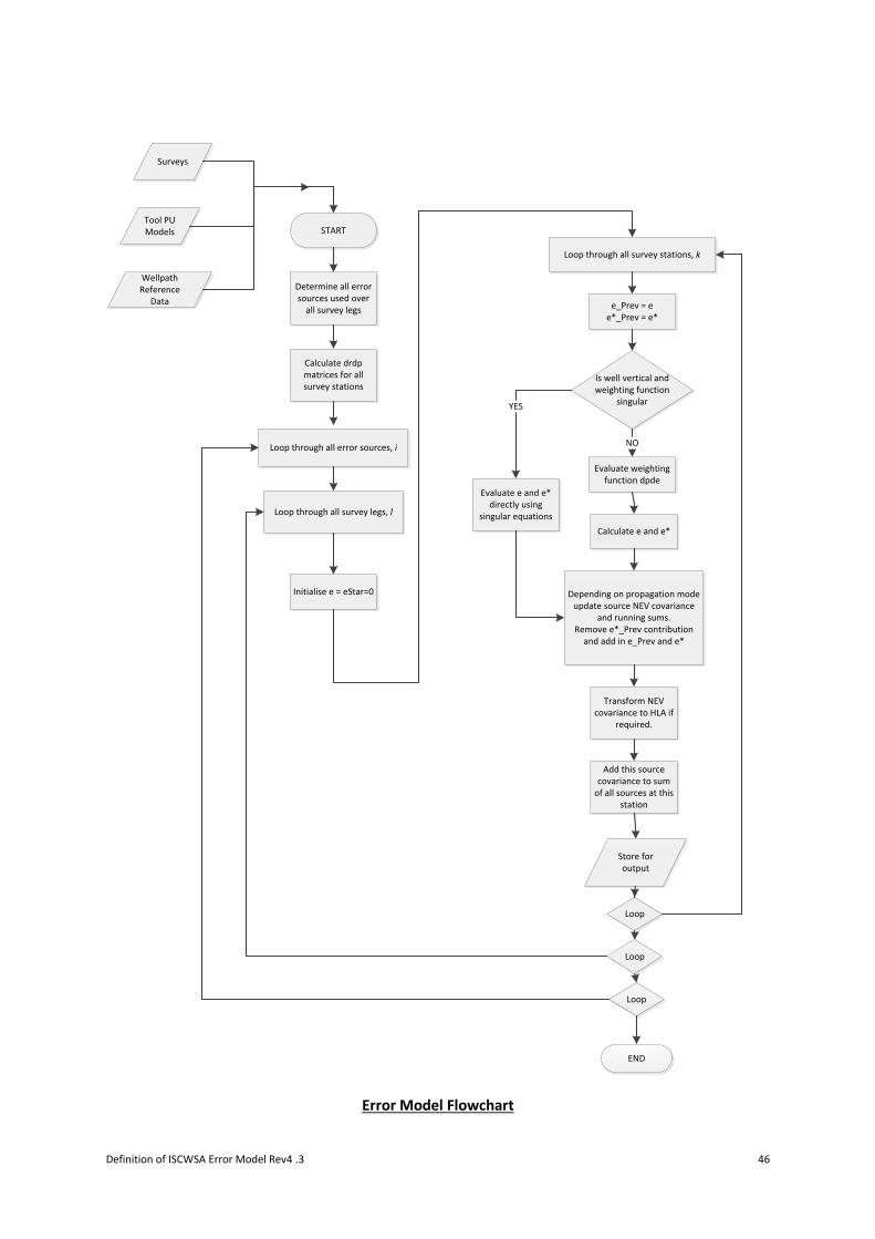
Definition of ISCWSA Error Model Rev4 .3 46
START
Surveys
Tool PU Models
Wellpath Reference
Data
Determine all error sources used over
all survey legs
Calculate drdp matrices for all survey stations
Loop through all error sources, i
Loop through all survey legs, l
Loop through all survey stations, k
Initialise e = eStar=0
e_Prev = ee*_Prev = e*
Evaluate weighting function dpde
Is well vertical and weighting function
singular
Calculate e and e*
Depending on propagation mode update source NEV covariance
and running sums.Remove e*_Prev contribution
and add in e_Prev and e*
Transform NEV covariance to HLA if
required.
Add this source covariance to sum
of all sources at this station
NO
Evaluate e and e* directly using
singular equations
YES
Loop
Loop
Loop
END
Store for output
Error Model Flowchart
Definition of ISCWSA Error Model Rev4 .3 47
9.4 Confidence Level
The error magnitudes defined in the MWD paper are all at one standard deviation (1-sigma). If the
user requires final error ellipses at two standard deviations (or three) then the 1-sigma ellipses can
simply be multiplied up and typically drilling software has a user control to define at what level error
ellipses are to be output. There are two provisos to this – some drilling software packages allow the
user to enter error magnitudes at different defined confidence levels (e.g. 1-sigma or 2-sigma etc.)
Also, the optional look up tables for the geo-magnetic reference terms require the user to define the
required output confidence level first so that certain magnetic field reference terms can be correctly
calculated (for further details see section §6.2.3 above.)
9.5 Example Implementation
As an example a series of Excel spreadsheets accompany this document. These evaluate the Rev4
MWD model on the three test wells and provide comparison of the output values at certain survey
stations with the diagnostic data at Copsegrove.com
All the errors are accumulated in covariance matrixes for each source and then these are
accumulated for the entire well.
Similar sheets are available for some of the gyro test cases. As per the test data in the gyro paper,
final covariance matrices in the nev axes (grid –nev) are calculated for a small number of survey
stations in each well.
In order to get close agreement with the test values provided in the gyro paper, the wellpath is
assumed to be defined to grid north, the curved sections of hole are defined at 10m interval and the
Md=0 station in the well is assumed to be a survey station with associated errors

Definition of ISCWSA Error Model Rev4 .3 48
10 References 1. Accuracy Prediction for Directional Measurement While Drilling
Hugh Williamson, SPE-67616
2. Prediction of Wellbore Position Accuracy When Surveyed with Gyroscopic Tools
Torgeir Torkildsen, Stein Harvardstein, John Weston, Roger Ekseth, SPE-90408
3. Quantification of Depth Accuracy A.Brooks, H Wilson, A.Jamieson, D.McRobbie, S.G.Holehouse SPE-95611
4. The Reliability Problem Related to Directional Survey Data
R.Ekseth, K.Kovalenko, J.L.Weston, T.Torkildsen, E.Nyrnes, A.Brooks and H.Wilson
ADC/SPE 103734, IADC/SPE Asia Pacific Drilling Technology Conference and Exhibition,
Bangkok, Thailand, 13-15 (Nov-2006)
5. High-Integrity Wellbore Surveys: Methods for Eliminating Gross Errors
R.Ekseth; T.Torkildsen; A.Brooks; J.Weston; E.Nyrnes; H.Wilson and K.Kovalenko
SPE/IADC 105558 SPE / IADC Drilling Conference, Amsterdam, The Netherlands, 20-22 (Feb
2007)
6. ISCWSA MWD Error Model Revisions
S. Grindrod, rev6 8/10/09 available at www.copesegrove.com
7. MWD Toolface Independent Error Terms
S. Grindrod CDR-SM-03 Rev4 November 2009 available at www.copesegrove.com
8. Confidence Limits Associated with Values of the Earth's Magnetic Field used for Directional
Drilling
Susan Macmillan, Allan McKay, Steve Grindrod SPE/IADC-119851
9. An Introduction to Wellbore Positioning
A.Jamieson et al., published by University of the Highland & Islands
10. Correct Vertical Well Weighting Functions for Cross-Axis Accelerometer Bias Terms
Chad Hanak, SuperiorQC LLC, January 28, 2016
11. A Comparison of Collision Avoidance Calculations
Shola Okewummi, Andrew Brooks SPE/IADC-140183
12. Borehole Position Uncertainty; Analysis of Measuring Methods and Derivation of
Systematic Error Model Chris J.M. Wolff and John P. DeWardt SPE-9223
13. Directional Surveying: Rotating and Sliding Operations Give Different Wellbore Position
Accuracy
Torgeir Torkildsen, Jon Bang, SPE 63275-MS, SPE ATCE, 1-4 October 2000, Dallas, Texas
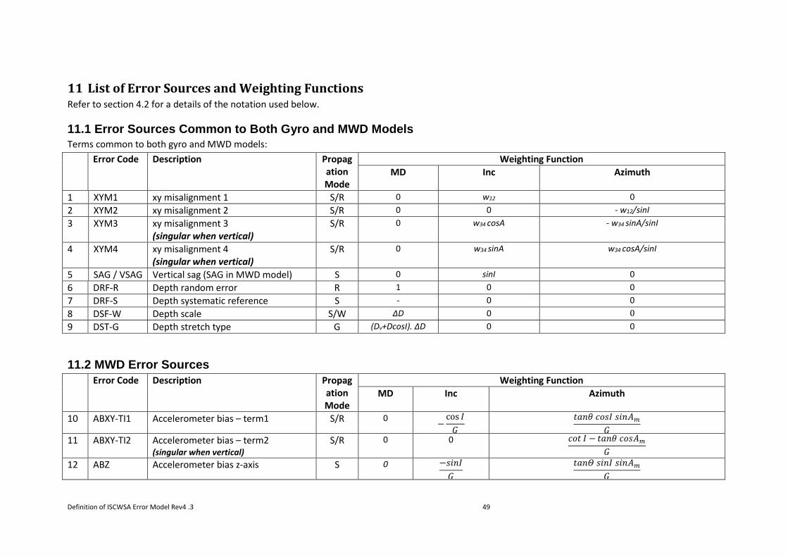
Definition of ISCWSA Error Model Rev4 .3 49
11 List of Error Sources and Weighting Functions Refer to section 4.2 for a details of the notation used below.
11.1 Error Sources Common to Both Gyro and MWD Models
Terms common to both gyro and MWD models:
Error Code Description Propagation Mode
Weighting Function
MD Inc Azimuth
1 XYM1 xy misalignment 1 S/R 0 w12 0
2 XYM2 xy misalignment 2 S/R 0 0 - w12/sinI
3 XYM3 xy misalignment 3 (singular when vertical)
S/R 0 w34 cosA - w34 sinA/sinI
4 XYM4 xy misalignment 4 (singular when vertical)
S/R 0 w34 sinA w34 cosA/sinI
5 SAG / VSAG Vertical sag (SAG in MWD model) S 0 sinI 0
6 DRF-R Depth random error R 1 0 0
7 DRF-S Depth systematic reference S - 0 0
8 DSF-W Depth scale S/W ΔD 0 0
9 DST-G Depth stretch type G (Dv+DcosI). ΔD 0 0
11.2 MWD Error Sources
Error Code Description Propagation Mode
Weighting Function
MD Inc Azimuth
10 ABXY-TI1 Accelerometer bias – term1 S/R 0 −
cos 𝐼
𝐺
𝑡𝑎𝑛𝜃 𝑐𝑜𝑠𝐼 𝑠𝑖𝑛𝐴𝑚
𝐺
11 ABXY-TI2 Accelerometer bias – term2 (singular when vertical)
S/R 0 0 𝑐𝑜𝑡 𝐼 − 𝑡𝑎𝑛𝜃 𝑐𝑜𝑠𝐴𝑚
𝐺
12 ABZ Accelerometer bias z-axis S 0 −𝑠𝑖𝑛𝐼
𝐺
𝑡𝑎𝑛𝛩 𝑠𝑖𝑛𝐼 𝑠𝑖𝑛𝐴𝑚
𝐺
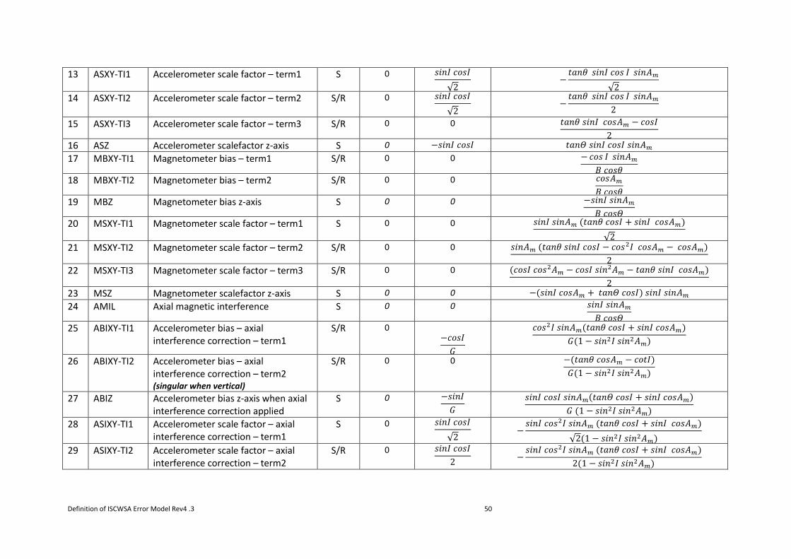
Definition of ISCWSA Error Model Rev4 .3 50
13 ASXY-TI1 Accelerometer scale factor – term1 S 0 𝑠𝑖𝑛𝐼 𝑐𝑜𝑠𝐼
√2 −
𝑡𝑎𝑛𝜃 𝑠𝑖𝑛𝐼 𝑐𝑜𝑠 𝐼 𝑠𝑖𝑛𝐴𝑚
√2
14 ASXY-TI2 Accelerometer scale factor – term2
S/R 0 𝑠𝑖𝑛𝐼 𝑐𝑜𝑠𝐼
√2 −
𝑡𝑎𝑛𝜃 𝑠𝑖𝑛𝐼 𝑐𝑜𝑠 𝐼 𝑠𝑖𝑛𝐴𝑚
2
15 ASXY-TI3 Accelerometer scale factor – term3 S/R 0 0 𝑡𝑎𝑛𝜃 𝑠𝑖𝑛𝐼 𝑐𝑜𝑠𝐴𝑚 − 𝑐𝑜𝑠𝐼
2
16 ASZ Accelerometer scalefactor z-axis S 0 −𝑠𝑖𝑛𝐼 𝑐𝑜𝑠𝐼 𝑡𝑎𝑛𝛩 𝑠𝑖𝑛𝐼 𝑐𝑜𝑠𝐼 𝑠𝑖𝑛𝐴𝑚
17 MBXY-TI1 Magnetometer bias – term1 S/R 0 0 −𝑐𝑜𝑠 𝐼 𝑠𝑖𝑛𝐴𝑚
𝐵 𝑐𝑜𝑠𝜃
18 MBXY-TI2 Magnetometer bias – term2 S/R 0 0 𝑐𝑜𝑠𝐴𝑚
𝐵 𝑐𝑜𝑠𝜃
19 MBZ Magnetometer bias z-axis S 0 0 −𝑠𝑖𝑛𝐼 𝑠𝑖𝑛𝐴𝑚
𝐵 𝑐𝑜𝑠𝛩
20 MSXY-TI1 Magnetometer scale factor – term1 S 0 0 𝑠𝑖𝑛𝐼 𝑠𝑖𝑛𝐴𝑚 (𝑡𝑎𝑛𝜃 𝑐𝑜𝑠𝐼 + 𝑠𝑖𝑛𝐼 𝑐𝑜𝑠𝐴𝑚)
√2
21 MSXY-TI2 Magnetometer scale factor – term2 S/R 0 0 𝑠𝑖𝑛𝐴𝑚 (𝑡𝑎𝑛𝜃 𝑠𝑖𝑛𝐼 𝑐𝑜𝑠𝐼 − 𝑐𝑜𝑠2𝐼 𝑐𝑜𝑠𝐴𝑚 − 𝑐𝑜𝑠𝐴𝑚)
2
22 MSXY-TI3 Magnetometer scale factor – term3 S/R 0 0 (𝑐𝑜𝑠𝐼 𝑐𝑜𝑠2𝐴𝑚 − 𝑐𝑜𝑠𝐼 𝑠𝑖𝑛2𝐴𝑚 − 𝑡𝑎𝑛𝜃 𝑠𝑖𝑛𝐼 𝑐𝑜𝑠𝐴𝑚)
2
23 MSZ Magnetometer scalefactor z-axis S 0 0 −(𝑠𝑖𝑛𝐼 𝑐𝑜𝑠𝐴𝑚 + 𝑡𝑎𝑛𝛩 𝑐𝑜𝑠𝐼) 𝑠𝑖𝑛𝐼 𝑠𝑖𝑛𝐴𝑚
24 AMIL Axial magnetic interference S 0 0 𝑠𝑖𝑛𝐼 𝑠𝑖𝑛𝐴𝑚
𝐵 𝑐𝑜𝑠𝛩
25 ABIXY-TI1 Accelerometer bias – axial interference correction – term1
S/R 0 −𝑐𝑜𝑠𝐼
𝐺
𝑐𝑜𝑠2𝐼 𝑠𝑖𝑛𝐴𝑚(𝑡𝑎𝑛𝜃 𝑐𝑜𝑠𝐼 + 𝑠𝑖𝑛𝐼 𝑐𝑜𝑠𝐴𝑚)
𝐺(1 − 𝑠𝑖𝑛2𝐼 𝑠𝑖𝑛2𝐴𝑚)
26 ABIXY-TI2 Accelerometer bias – axial interference correction – term2 (singular when vertical)
S/R 0 0 −(𝑡𝑎𝑛𝜃 𝑐𝑜𝑠𝐴𝑚 − 𝑐𝑜𝑡𝐼)
𝐺(1 − 𝑠𝑖𝑛2𝐼 𝑠𝑖𝑛2𝐴𝑚)
27 ABIZ Accelerometer bias z-axis when axial interference correction applied
S 0 −𝑠𝑖𝑛𝐼
𝐺
𝑠𝑖𝑛𝐼 𝑐𝑜𝑠𝐼 𝑠𝑖𝑛𝐴𝑚(𝑡𝑎𝑛𝛩 𝑐𝑜𝑠𝐼 + 𝑠𝑖𝑛𝐼 𝑐𝑜𝑠𝐴𝑚)
𝐺 (1 − 𝑠𝑖𝑛2𝐼 𝑠𝑖𝑛2𝐴𝑚)
28 ASIXY-TI1 Accelerometer scale factor – axial interference correction – term1
S 0 𝑠𝑖𝑛𝐼 𝑐𝑜𝑠𝐼
√2 −
𝑠𝑖𝑛𝐼 𝑐𝑜𝑠2𝐼 𝑠𝑖𝑛𝐴𝑚 (𝑡𝑎𝑛𝜃 𝑐𝑜𝑠𝐼 + 𝑠𝑖𝑛𝐼 𝑐𝑜𝑠𝐴𝑚)
√2(1 − 𝑠𝑖𝑛2𝐼 𝑠𝑖𝑛2𝐴𝑚)
29 ASIXY-TI2 Accelerometer scale factor – axial interference correction – term2
S/R 0 𝑠𝑖𝑛𝐼 𝑐𝑜𝑠𝐼
2 −
𝑠𝑖𝑛𝐼 𝑐𝑜𝑠2𝐼 𝑠𝑖𝑛𝐴𝑚 (𝑡𝑎𝑛𝜃 𝑐𝑜𝑠𝐼 + 𝑠𝑖𝑛𝐼 𝑐𝑜𝑠𝐴𝑚)
2(1 − 𝑠𝑖𝑛2𝐼 𝑠𝑖𝑛2𝐴𝑚)
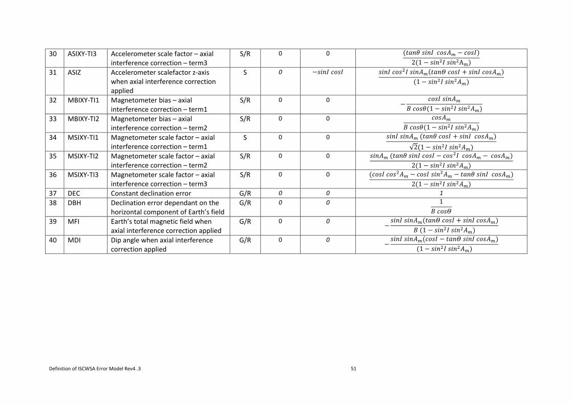
Definition of ISCWSA Error Model Rev4 .3 51
30 ASIXY-TI3 Accelerometer scale factor – axial interference correction – term3
S/R 0 0 (𝑡𝑎𝑛𝜃 𝑠𝑖𝑛𝐼 𝑐𝑜𝑠𝐴𝑚 − 𝑐𝑜𝑠𝐼)
2(1 − 𝑠𝑖𝑛2𝐼 𝑠𝑖𝑛2Am)
31 ASIZ Accelerometer scalefactor z-axis when axial interference correction applied
S 0 −𝑠𝑖𝑛𝐼 𝑐𝑜𝑠𝐼 𝑠𝑖𝑛𝐼 𝑐𝑜𝑠2𝐼 𝑠𝑖𝑛𝐴𝑚(𝑡𝑎𝑛𝛩 𝑐𝑜𝑠𝐼 + 𝑠𝑖𝑛𝐼 𝑐𝑜𝑠𝐴𝑚)
(1 − 𝑠𝑖𝑛2𝐼 𝑠𝑖𝑛2𝐴𝑚)
32 MBIXY-TI1 Magnetometer bias – axial interference correction – term1
S/R 0 0 −
𝑐𝑜𝑠𝐼 𝑠𝑖𝑛𝐴𝑚
𝐵 𝑐𝑜𝑠𝜃(1 − 𝑠𝑖𝑛2𝐼 𝑠𝑖𝑛2𝐴𝑚)
33 MBIXY-TI2 Magnetometer bias – axial interference correction – term2
S/R 0 0 𝑐𝑜𝑠𝐴𝑚
𝐵 𝑐𝑜𝑠𝜃(1 − 𝑠𝑖𝑛2𝐼 𝑠𝑖𝑛2𝐴𝑚)
34 MSIXY-TI1 Magnetometer scale factor – axial interference correction – term1
S 0 0 𝑠𝑖𝑛𝐼 𝑠𝑖𝑛𝐴𝑚 (𝑡𝑎𝑛𝜃 𝑐𝑜𝑠𝐼 + 𝑠𝑖𝑛𝐼 𝑐𝑜𝑠𝐴𝑚)
√2(1 − 𝑠𝑖𝑛2𝐼 𝑠𝑖𝑛2𝐴𝑚)
35 MSIXY-TI2 Magnetometer scale factor – axial interference correction – term2
S/R 0 0 𝑠𝑖𝑛𝐴𝑚 (𝑡𝑎𝑛𝜃 𝑠𝑖𝑛𝐼 𝑐𝑜𝑠𝐼 − 𝑐𝑜𝑠2𝐼 𝑐𝑜𝑠𝐴𝑚 − 𝑐𝑜𝑠𝐴𝑚)
2(1 − 𝑠𝑖𝑛2𝐼 𝑠𝑖𝑛2𝐴𝑚)
36 MSIXY-TI3 Magnetometer scale factor – axial interference correction – term3
S/R 0 0 (𝑐𝑜𝑠𝐼 𝑐𝑜𝑠2𝐴𝑚 − 𝑐𝑜𝑠𝐼 𝑠𝑖𝑛2𝐴𝑚 − 𝑡𝑎𝑛𝜃 𝑠𝑖𝑛𝐼 𝑐𝑜𝑠𝐴𝑚)
2(1 − 𝑠𝑖𝑛2𝐼 𝑠𝑖𝑛2𝐴𝑚)
37 DEC Constant declination error G/R 0 0 1
38 DBH Declination error dependant on the horizontal component of Earth’s field
G/R 0 0 1
𝐵 𝑐𝑜𝑠𝛩
39 MFI Earth’s total magnetic field when axial interference correction applied
G/R 0 0 −
𝑠𝑖𝑛𝐼 𝑠𝑖𝑛𝐴𝑚(𝑡𝑎𝑛𝛩 𝑐𝑜𝑠𝐼 + 𝑠𝑖𝑛𝐼 𝑐𝑜𝑠𝐴𝑚)
𝐵 (1 − 𝑠𝑖𝑛2𝐼 𝑠𝑖𝑛2𝐴𝑚)
40 MDI Dip angle when axial interference correction applied
G/R 0 0 −
𝑠𝑖𝑛𝐼 𝑠𝑖𝑛𝐴𝑚(𝑐𝑜𝑠𝐼 − 𝑡𝑎𝑛𝛩 𝑠𝑖𝑛𝐼 𝑐𝑜𝑠𝐴𝑚)
(1 − 𝑠𝑖𝑛2𝐼 𝑠𝑖𝑛2𝐴𝑚)

Definition of ISCWSA Error Model Rev4 .3 52
11.3 Gyro Error Sources
For the gyro model, the error sources may be grouped depending on the tool sensor configuration and further split into those which apply in Stationary
survey mode, Continuous survey mode or either mode. During a single survey leg a tool made transition between these modes as a function of inclination.
Error Code Description SurveyMode
Propagation Mode
Weighting Function
MD Inc Azimuth
41 AXYZ-XYB 3-axis: xy accelerometer bias C/S S/R 0 cos 𝐼
𝐺
0
42 AXYZ-ZB 3-axis: z accelerometer bias C/S S 0 sin 𝐼
𝐺
0
43 AXYZ-SF 3-axis: accelerometer scale factor error C/S S 0 1 3 sinI cosI 0
44 AXYZ-MIS 3-axis: accelerometer misalignment C/S S 0 1 0
45 AXY-B 2-axis: xy accelerometer bias C/S S/R 0 1
𝐺𝑐𝑜𝑠(𝐼 − 𝑘 𝛾)
0
46 AXY-SF 2-axis: Accelerometer scale factor error C/S S 0 tan (𝐼 − 𝑘 𝛾) 0
47 AXY-MS 2-axis: Accelerometer misalignment C/S S 0 1 0
48 AXY-GB 2-axis: Gravity Bias C/S S 0 tan (𝐼 − 𝑘 𝛾)
𝐺
0
49 GXYZ-XYB1 3-axis, stationary: xy gyro bias 1 S S/R 0 0 𝑠𝑖𝑛𝐴𝑇 𝑐𝑜𝑠𝐼
Ωcosϕ
50 GXYZ-XYB2 3-axis, stationary: xy gyro bias 2 S S/R 0 0 𝑐𝑜𝑠𝐴𝑇
Ωcosϕ
51 GXYZ-XYRN 3-axis, stationary: xy gyro random noise S R 0 0 𝑓
√1 − 𝑠𝑖𝑛2𝐴𝑇 𝑠𝑖𝑛2𝐼
Ωcosϕ
52 GXYZ-XYG1 3-axis, stationary: xy gyro g-dependent error 1
S S 0 0 𝑐𝑜𝑠𝐴𝑇𝑠𝑖𝑛𝐼
Ωcosϕ
53 GXYZ-XYG2 3-axis, stationary: xy gyro g-dependent error 2
S S/R 0 0 𝑐𝑜𝑠𝐴𝑇 𝑐𝑜𝑠𝐼
Ωcosϕ
54 GXYZ-XYG3 3-axis, stationary: xy gyro g-dependent error 3
S S/R 0 0 𝑠𝑖𝑛𝐴𝑇 𝑐𝑜𝑠2𝐼
Ωcosϕ
55 GXYZ-XYG4 3-axis, stationary: xy gyro g-dependent error 4
S S 0 0 𝑠𝑖𝑛𝐴𝑇 𝑠𝑖𝑛𝐼 𝑐𝑜𝑠𝐼
Ωcosϕ
56 GXYZ-ZB 3-axis, stationary: z gyro bias S S 0 0 𝑠𝑖𝑛𝐴𝑇 𝑠𝑖𝑛𝐼
Ωcosϕ
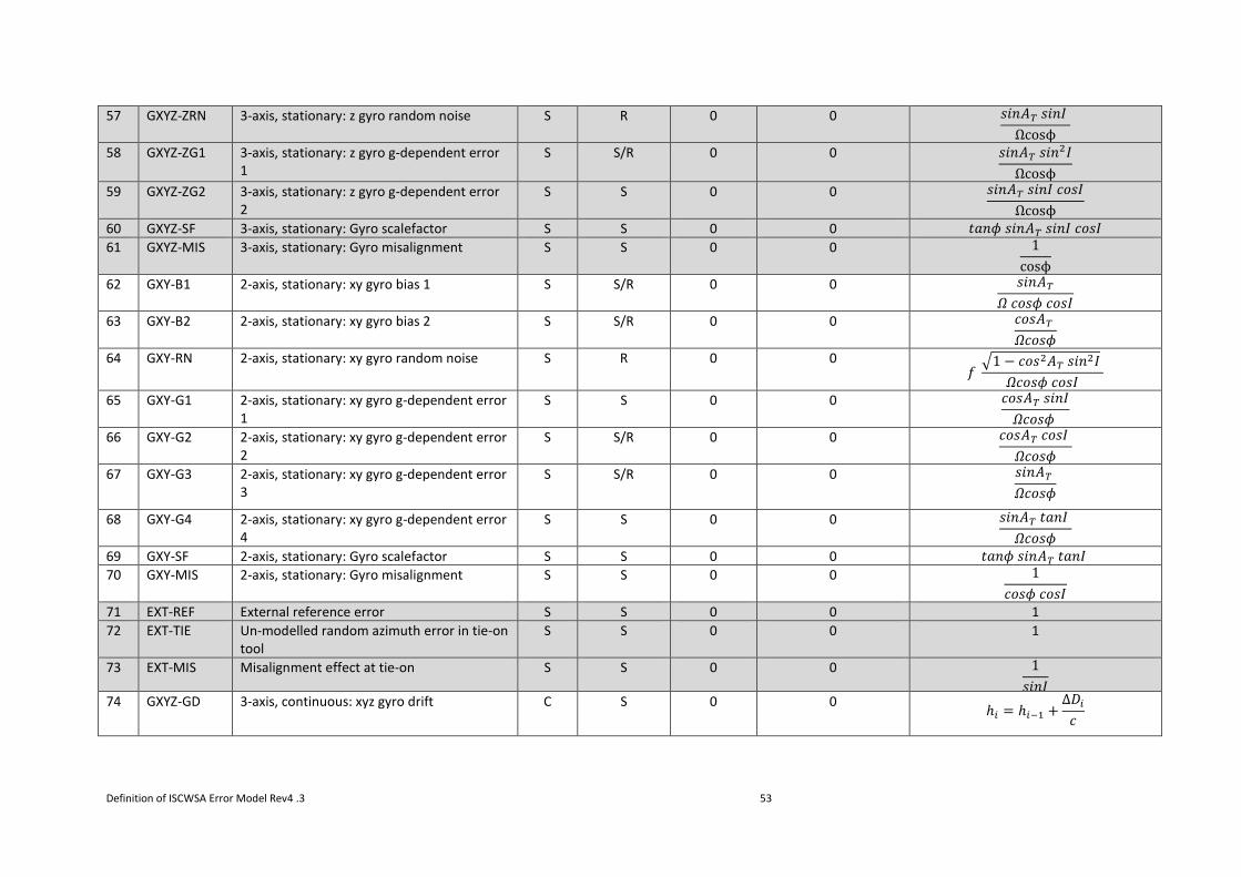
Definition of ISCWSA Error Model Rev4 .3 53
57 GXYZ-ZRN 3-axis, stationary: z gyro random noise S R 0 0 𝑠𝑖𝑛𝐴𝑇 𝑠𝑖𝑛𝐼
Ωcosϕ
58 GXYZ-ZG1 3-axis, stationary: z gyro g-dependent error 1
S S/R 0 0 𝑠𝑖𝑛𝐴𝑇 𝑠𝑖𝑛2𝐼
Ωcosϕ
59 GXYZ-ZG2 3-axis, stationary: z gyro g-dependent error 2
S S 0 0 𝑠𝑖𝑛𝐴𝑇 𝑠𝑖𝑛𝐼 𝑐𝑜𝑠𝐼
Ωcosϕ
60 GXYZ-SF 3-axis, stationary: Gyro scalefactor S S 0 0 𝑡𝑎𝑛𝜙 𝑠𝑖𝑛𝐴𝑇 𝑠𝑖𝑛𝐼 𝑐𝑜𝑠𝐼
61 GXYZ-MIS 3-axis, stationary: Gyro misalignment S S 0 0 1
cosϕ
62 GXY-B1 2-axis, stationary: xy gyro bias 1 S S/R 0 0 𝑠𝑖𝑛𝐴𝑇
𝛺 𝑐𝑜𝑠𝜙 𝑐𝑜𝑠𝐼
63 GXY-B2 2-axis, stationary: xy gyro bias 2 S S/R 0 0 𝑐𝑜𝑠𝐴𝑇
𝛺𝑐𝑜𝑠𝜙
64 GXY-RN 2-axis, stationary: xy gyro random noise S R 0 0 𝑓
√1 − 𝑐𝑜𝑠2𝐴𝑇 𝑠𝑖𝑛2𝐼
𝛺𝑐𝑜𝑠𝜙 𝑐𝑜𝑠𝐼
65 GXY-G1 2-axis, stationary: xy gyro g-dependent error 1
S S 0 0 𝑐𝑜𝑠𝐴𝑇 𝑠𝑖𝑛𝐼
𝛺𝑐𝑜𝑠𝜙
66 GXY-G2 2-axis, stationary: xy gyro g-dependent error 2
S S/R 0 0 𝑐𝑜𝑠𝐴𝑇 𝑐𝑜𝑠𝐼
𝛺𝑐𝑜𝑠𝜙
67 GXY-G3 2-axis, stationary: xy gyro g-dependent error 3
S S/R 0 0 𝑠𝑖𝑛𝐴𝑇
𝛺𝑐𝑜𝑠𝜙
68 GXY-G4 2-axis, stationary: xy gyro g-dependent error 4
S S 0 0 𝑠𝑖𝑛𝐴𝑇 𝑡𝑎𝑛𝐼
𝛺𝑐𝑜𝑠𝜙
69 GXY-SF 2-axis, stationary: Gyro scalefactor S S 0 0 𝑡𝑎𝑛𝜙 𝑠𝑖𝑛𝐴𝑇 𝑡𝑎𝑛𝐼
70 GXY-MIS 2-axis, stationary: Gyro misalignment S S 0 0 1
𝑐𝑜𝑠𝜙 𝑐𝑜𝑠𝐼
71 EXT-REF External reference error S S 0 0 1
72 EXT-TIE Un-modelled random azimuth error in tie-on tool
S S 0 0 1
73 EXT-MIS Misalignment effect at tie-on S S 0 0 1
𝑠𝑖𝑛𝐼
74 GXYZ-GD 3-axis, continuous: xyz gyro drift C S 0 0 ℎ𝑖 = ℎ𝑖−1 +
∆𝐷𝑖
𝑐
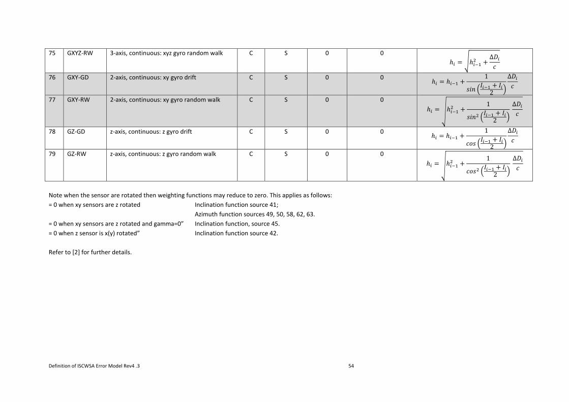
Definition of ISCWSA Error Model Rev4 .3 54
75 GXYZ-RW 3-axis, continuous: xyz gyro random walk C S 0 0
ℎ𝑖 = √ℎ𝑖−12 +
∆𝐷𝑖
𝑐
76 GXY-GD 2-axis, continuous: xy gyro drift C S 0 0 ℎ𝑖 = ℎ𝑖−1 +
1
𝑠𝑖𝑛 (𝐼𝑖−1 + 𝐼𝑖
2)
∆𝐷𝑖
𝑐
77 GXY-RW 2-axis, continuous: xy gyro random walk C S 0 0
ℎ𝑖 = √ℎ𝑖−12 +
1
𝑠𝑖𝑛2 (𝐼𝑖−1 + 𝐼𝑖
2) ∆𝐷𝑖
𝑐
78 GZ-GD z-axis, continuous: z gyro drift C S 0 0 ℎ𝑖 = ℎ𝑖−1 +
1
𝑐𝑜𝑠 (𝐼𝑖−1 + 𝐼𝑖
2)
∆𝐷𝑖
𝑐
79 GZ-RW z-axis, continuous: z gyro random walk C S 0 0
ℎ𝑖 = √ℎ𝑖−12 +
1
𝑐𝑜𝑠2 (𝐼𝑖−1 + 𝐼𝑖
2) ∆𝐷𝑖
𝑐
Note when the sensor are rotated then weighting functions may reduce to zero. This applies as follows:
= 0 when xy sensors are z rotated Inclination function source 41;
Azimuth function sources 49, 50, 58, 62, 63.
= 0 when xy sensors are z rotated and gamma=0” Inclination function, source 45.
= 0 when z sensor is x(y) rotated” Inclination function source 42.
Refer to [2] for further details.

Definition of ISCWSA Error Model Rev4 .3 55
11.4 Utility Sources
The following sources do not represent any clear physical source of error, in Blind and Unknown tool modelling to guestimate position uncertainty.
Alternatively, the effect of CNA and CNI can be represented using misalignment terms.
80 CNA Linear Cone – Inclination C S 0 0 ℎ𝑖 =
1
sinI
81 CNI Linear Cone - Azimuth C S 0 1 0
11.5 Vertical Singularities
Several of the functions above are singular in vertical hole. The following formula may be substituted when vertical.
North Formula East Formula Vertical Formula
3v XYM3 xy misalignment 3 (singular when vertical)
1 0 0
4v XYM4 xy misalignment 4 (singular when vertical)
0 1 0
11v ABXY-TI2 Accelerometer bias – term2 (singular when vertical)
-sinAm/G cosAm/G 0
20v ABIXY-TI2 Accelerometer bias – axial interference correction – term2 (singular when vertical)
-sinAm/G cosAm/G 0
80v CNA Linear Cone – Inclination (singular when vertical)
-sin(Az) Cos(Az) 0
Note. XYM2 is also singular when vertical is misalignment option 1 is used. However as noted in the [2] in this situation this term may give
strange/unwanted values when azimuth or toolface vary.
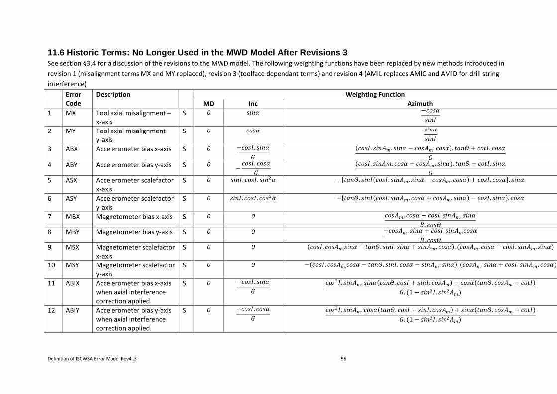
Definition of ISCWSA Error Model Rev4 .3 56
11.6 Historic Terms: No Longer Used in the MWD Model After Revisions 3
See section §3.4 for a discussion of the revisions to the MWD model. The following weighting functions have been replaced by new methods introduced in
revision 1 (misalignment terms MX and MY replaced), revision 3 (toolface dependant terms) and revision 4 (AMIL replaces AMIC and AMID for drill string
interference)
Error Code
Description Weighting Function
MD Inc Azimuth
1 MX Tool axial misalignment – x-axis
S 0 𝑠𝑖𝑛𝛼 −𝑐𝑜𝑠𝛼
𝑠𝑖𝑛𝐼
2 MY Tool axial misalignment – y-axis
S 0 𝑐𝑜𝑠𝛼 𝑠𝑖𝑛𝛼
𝑠𝑖𝑛𝐼
3 ABX Accelerometer bias x-axis S 0 −𝑐𝑜𝑠𝐼. 𝑠𝑖𝑛𝛼
𝐺
(𝑐𝑜𝑠𝐼. 𝑠𝑖𝑛𝐴𝑚. 𝑠𝑖𝑛𝛼 − 𝑐𝑜𝑠𝐴𝑚. 𝑐𝑜𝑠𝛼). 𝑡𝑎𝑛𝛩 + 𝑐𝑜𝑡𝐼. 𝑐𝑜𝑠𝛼
𝐺
4 ABY Accelerometer bias y-axis S 0 −
𝑐𝑜𝑠𝐼. 𝑐𝑜𝑠𝛼
𝐺
(𝑐𝑜𝑠𝐼. 𝑠𝑖𝑛𝐴𝑚. 𝑐𝑜𝑠𝛼 + 𝑐𝑜𝑠𝐴𝑚. 𝑠𝑖𝑛𝛼). 𝑡𝑎𝑛𝛩 − 𝑐𝑜𝑡𝐼. 𝑠𝑖𝑛𝛼
𝐺
5 ASX Accelerometer scalefactor x-axis
S 0 𝑠𝑖𝑛𝐼. 𝑐𝑜𝑠𝐼. 𝑠𝑖𝑛2𝛼 −{𝑡𝑎𝑛𝛩. 𝑠𝑖𝑛𝐼(𝑐𝑜𝑠𝐼. 𝑠𝑖𝑛𝐴𝑚. 𝑠𝑖𝑛𝛼 − 𝑐𝑜𝑠𝐴𝑚. 𝑐𝑜𝑠𝛼) + 𝑐𝑜𝑠𝐼. 𝑐𝑜𝑠𝛼}. 𝑠𝑖𝑛𝛼
6 ASY Accelerometer scalefactor y-axis
S 0 𝑠𝑖𝑛𝐼. 𝑐𝑜𝑠𝐼. 𝑐𝑜𝑠2𝛼 −{𝑡𝑎𝑛𝛩. 𝑠𝑖𝑛𝐼(𝑐𝑜𝑠𝐼. 𝑠𝑖𝑛𝐴𝑚. 𝑐𝑜𝑠𝛼 + 𝑐𝑜𝑠𝐴𝑚. 𝑠𝑖𝑛𝛼) − 𝑐𝑜𝑠𝐼. 𝑠𝑖𝑛𝛼}. 𝑐𝑜𝑠𝛼
7 MBX Magnetometer bias x-axis S 0 0 𝑐𝑜𝑠𝐴𝑚. 𝑐𝑜𝑠𝛼 − 𝑐𝑜𝑠𝐼. 𝑠𝑖𝑛𝐴𝑚. 𝑠𝑖𝑛𝛼
𝐵. 𝑐𝑜𝑠𝛩
8 MBY Magnetometer bias y-axis S 0 0 −𝑐𝑜𝑠𝐴𝑚. 𝑠𝑖𝑛𝛼 + 𝑐𝑜𝑠𝐼. 𝑠𝑖𝑛𝐴𝑚𝑐𝑜𝑠𝛼
𝐵. 𝑐𝑜𝑠𝛩
9 MSX Magnetometer scalefactor x-axis
S 0 0 (𝑐𝑜𝑠𝐼. 𝑐𝑜𝑠𝐴𝑚.𝑠𝑖𝑛𝛼 − 𝑡𝑎𝑛𝛩. 𝑠𝑖𝑛𝐼. 𝑠𝑖𝑛𝛼 + 𝑠𝑖𝑛𝐴𝑚. 𝑐𝑜𝑠𝛼). (𝑐𝑜𝑠𝐴𝑚. 𝑐𝑜𝑠𝛼 − 𝑐𝑜𝑠𝐼. 𝑠𝑖𝑛𝐴𝑚. 𝑠𝑖𝑛𝛼)
10 MSY Magnetometer scalefactor y-axis
S 0 0 −(𝑐𝑜𝑠𝐼. 𝑐𝑜𝑠𝐴𝑚.𝑐𝑜𝑠𝛼 − 𝑡𝑎𝑛𝛩. 𝑠𝑖𝑛𝐼. 𝑐𝑜𝑠𝛼 − 𝑠𝑖𝑛𝐴𝑚. 𝑠𝑖𝑛𝛼). (𝑐𝑜𝑠𝐴𝑚. 𝑠𝑖𝑛𝛼 + 𝑐𝑜𝑠𝐼. 𝑠𝑖𝑛𝐴𝑚. 𝑐𝑜𝑠𝛼)
11 ABIX Accelerometer bias x-axis when axial interference correction applied.
S 0 −𝑐𝑜𝑠𝐼. 𝑠𝑖𝑛𝛼
𝐺
𝑐𝑜𝑠2𝐼. 𝑠𝑖𝑛𝐴𝑚. 𝑠𝑖𝑛𝛼(𝑡𝑎𝑛𝛩. 𝑐𝑜𝑠𝐼 + 𝑠𝑖𝑛𝐼. 𝑐𝑜𝑠𝐴𝑚) − 𝑐𝑜𝑠𝛼(𝑡𝑎𝑛𝛩. 𝑐𝑜𝑠𝐴𝑚 − 𝑐𝑜𝑡𝐼)
𝐺. (1 − 𝑠𝑖𝑛2𝐼. 𝑠𝑖𝑛2𝐴𝑚)
12 ABIY Accelerometer bias y-axis when axial interference correction applied.
S 0 −𝑐𝑜𝑠𝐼. 𝑐𝑜𝑠𝛼
𝐺
𝑐𝑜𝑠2𝐼. 𝑠𝑖𝑛𝐴𝑚. 𝑐𝑜𝑠𝛼(𝑡𝑎𝑛𝛩. 𝑐𝑜𝑠𝐼 + 𝑠𝑖𝑛𝐼. 𝑐𝑜𝑠𝐴𝑚) + 𝑠𝑖𝑛𝛼(𝑡𝑎𝑛𝛩. 𝑐𝑜𝑠𝐴𝑚 − 𝑐𝑜𝑡𝐼)
𝐺. (1 − 𝑠𝑖𝑛2𝐼. 𝑠𝑖𝑛2𝐴𝑚)

Definition of ISCWSA Error Model Rev4 .3 57
13 ASIX Accelerometer scalefactor x-axis when axial interference correction applied.
S 0 𝑠𝑖𝑛𝐼. 𝑐𝑜𝑠𝐼. 𝑠𝑖𝑛2𝛼 −𝑠𝑖𝑛𝛼[𝑠𝑖𝑛𝐼. 𝑐𝑜𝑠2𝐼. 𝑠𝑖𝑛𝐴𝑚. 𝑠𝑖𝑛𝛼(𝑡𝑎𝑛𝛩. 𝑐𝑜𝑠𝐼 + 𝑠𝑖𝑛𝐼. 𝑐𝑜𝑠𝐴𝑚) − 𝑐𝑜𝑠𝛼(𝑡𝑎𝑛𝛩. 𝑠𝑖𝑛𝐼. 𝑐𝑜𝑠𝐴𝑚 − 𝑐𝑜𝑠𝐼)]
(1 − 𝑠𝑖𝑛2𝐼. 𝑠𝑖𝑛2𝐴𝑚)
14 ASIY Accelerometer scalefactor y-axis when axial interference correction applied.
S 0 𝑠𝑖𝑛𝐼. 𝑐𝑜𝑠𝐼. 𝑐𝑜𝑠2𝛼 −𝑐𝑜𝑠𝛼[𝑠𝑖𝑛𝐼. 𝑐𝑜𝑠2𝐼. 𝑠𝑖𝑛𝐴𝑚. 𝑐𝑜𝑠𝛼(𝑡𝑎𝑛𝛩. 𝑐𝑜𝑠𝐼 + 𝑠𝑖𝑛𝐼. 𝑐𝑜𝑠𝐴𝑚) + 𝑠𝑖𝑛𝛼(𝑡𝑎𝑛𝛩. 𝑠𝑖𝑛𝐼. 𝑐𝑜𝑠𝐴𝑚 − 𝑐𝑜𝑠𝐼)]
(1 − 𝑠𝑖𝑛2𝐼. 𝑠𝑖𝑛2𝐴𝑚)
15 MBIX Magnetometer bias x-axis when axial interference correction applied.
S 0 0 −
𝑐𝑜𝑠𝐼. 𝑠𝑖𝑛𝐴𝑚𝑠𝑖𝑛𝛼 − 𝑐𝑜𝑠𝐴𝑚𝑐𝑜𝑠𝛼
𝐵𝑐𝑜𝑠𝛩. (1 − 𝑠𝑖𝑛2𝐼. 𝑠𝑖𝑛2𝐴𝑚)
16 MBIY Magnetometer bias y-axis when axial interference correction applied.
S 0 0 −
𝑐𝑜𝑠𝐼. 𝑠𝑖𝑛𝐴𝑚𝑐𝑜𝑠𝛼 + 𝑐𝑜𝑠𝐴𝑚𝑠𝑖𝑛𝛼
𝐵𝑐𝑜𝑠𝛩. (1 − 𝑠𝑖𝑛2𝐼. 𝑠𝑖𝑛2𝐴𝑚)
17 MSIX Magnetometer scalefactor x-axis when axial interference correction applied.
S 0 0 −
(𝑐𝑜𝑠𝐼. 𝑐𝑜𝑠𝐴𝑚𝑠𝑖𝑛𝛼 − 𝑡𝑎𝑛𝛩. 𝑠𝑖𝑛𝐼. 𝑠𝑖𝑛𝛼 + 𝑠𝑖𝑛𝐴𝑚𝑐𝑜𝑠𝛼)(𝑐𝑜𝑠𝐼. 𝑠𝑖𝑛𝐴𝑚𝑠𝑖𝑛𝛼 − 𝑐𝑜𝑠𝐴𝑚𝑐𝑜𝑠𝛼)
(1 − 𝑠𝑖𝑛2𝐼. 𝑠𝑖𝑛2𝐴𝑚)
18 MSIY Magnetometer scalefactor y-axis when axial interference correction applied.
S 0 0 −
(𝑐𝑜𝑠𝐼. 𝑐𝑜𝑠𝐴𝑚𝑐𝑜𝑠𝛼 − 𝑡𝑎𝑛𝛩. 𝑠𝑖𝑛𝐼. 𝑐𝑜𝑠𝛼 − 𝑠𝑖𝑛𝐴𝑚𝑠𝑖𝑛𝛼)(𝑐𝑜𝑠𝐼. 𝑠𝑖𝑛𝐴𝑚𝑐𝑜𝑠𝛼 + 𝑐𝑜𝑠𝐴𝑚𝑠𝑖𝑛𝛼)
(1 − 𝑠𝑖𝑛2𝐼. 𝑠𝑖𝑛2𝐴𝑚)
18 AMIC Constant axial magnetic interference
S 0 0 1
19 AMID Direction dependant axial magnetic interference
S 0 0 𝑠𝑖𝑛𝐼. 𝑠𝑖𝑛𝐴𝑚